3.1. Front-tracking method

The numerical study is performed using the open source TrioCFD software within the TRUST HPC platform (Calvin, Cueto & Emonot Reference Calvin, Cueto and Emonot2002; Saikali et al. Reference Saikali, Ledac, Bruneton, Khizar, Bourcier, Bernard-Michel, Adam and Houssin-Agbomson2021). Based on an object oriented design, the code is massively parallel and is written in modern C++ language.

A two-phase flow module, based on a discontinuous front-tracking (DFT) method (Mathieu Reference Mathieu2003), is employed. In this method the interface between two fluid phases is defined as moving connected-marker points (Lagrangian grid), independent from the Eulerian grid used to mesh the computational domain. On the Eulerian mesh, one-fluid velocity and pressure fields are considered for both phases and updated by solving the Navier–Stokes equations. The markers of the moving Lagrangian grid are, for their part, advected by the velocity field of the Eulerian mesh as described in du Cluzeau, Bois & Toutant (Reference du Cluzeau, Bois and Toutant2019). The phase indicator function, and thus, the physical properties of each phase (density and viscosity) are finally updated using the new marker positions.

The discretisation in space is performed by a mixed finite difference/volume method that is implemented on a staggered Eulerian grid of type marker and cell. Spatial derivatives are discretised with a classical second-order centred scheme.

A first order semi-implicit time integration scheme (matrix free) is employed where the diffusion terms are treated implicitly, while the convective terms are explicitly considered. As a consequence, the time step is dynamically selected at each iteration respecting the Courant–Friedrichs–Lewy (CFL) criterion, thus ensuring the stability of the numerical scheme. However, this criterion does not enforce stability for the Lagrangian grid motion and time steps must be limited by a maximum value, which needs to be chosen following a convergence study (§ 3.4). The linear system of equations resulting from the implicit treatment of the diffusion terms is solved (Saad Reference Saad2003) by the conjugate gradient method (CGM). The library PETSc (2024) is used for this purpose.

To handle the velocity–pressure coupling, a projection method is used satisfying the mass conservation equation. The resulting elliptic pressure Poisson equation is solved with CGM and symmetric successive over-relaxation preconditioning. More technical details on the algorithm are given by Saikali (Reference Saikali2018).

3.2. Governing equations for numerical treatment

The one-fluid equations of Kataoka (Reference Kataoka1986) solved by TrioCFD are

(3.1)$$\begin{gather} \boldsymbol{\nabla}\boldsymbol{\cdot}\boldsymbol{v} = 0, \end{gather}$$

(3.2)$$\begin{gather}\frac{\partial \rho\boldsymbol{v}}{\partial t}+\boldsymbol{\nabla}\boldsymbol{\cdot} ( \rho\boldsymbol{v}\times\boldsymbol{v})={-}\boldsymbol{\nabla} P+\boldsymbol{\nabla}\boldsymbol{\cdot}[ \mu( \boldsymbol{\nabla}\boldsymbol{v}+ \boldsymbol{\nabla}^T\boldsymbol{v})]+\sigma\kappa\boldsymbol{n}\delta^i, \end{gather}$$

where the one-fluid variables are obtained from their values in each phase: ${\phi =\chi _g \phi _g+\chi _l \phi _l}$ with $\phi _k$ either the velocity ($\boldsymbol {v_k}$), pressure ($P_k$), density ($\rho _k$) or viscosity ($\mu _k$) of the fluid $k={l,g}$. Here $\chi _k$ is the phase indicator function, equal to 1 in phase $k$ and 0 elsewhere. The gas phase indicator $\chi _g$ is transported through $\partial \chi _g/\partial t+\boldsymbol {v}_i\boldsymbol {\cdot }\boldsymbol {\nabla }\chi _g=0$, where $\boldsymbol {v}_i=\boldsymbol {v}(R_i)$ is the interfacial velocity. In the absence of phase change, the velocity is continuous across the interface. Here $\sigma$ is the surface tension, $\kappa =-\boldsymbol {\nabla }\boldsymbol {\cdot }\boldsymbol {n}$ the local curvature and $\boldsymbol {n}$ the interface normal directed towards the core fluid and defined by $\boldsymbol {\nabla }\chi _l=-\boldsymbol {n}\delta ^i$, where $\delta ^i$ is the Dirac delta function centred at the interface.

3.3. Initial and boundary conditions

Boundary conditions are required for both the Eulerian fixed mesh (pressure or velocity) and the Lagrangian mesh (interface). For the former, zero velocities are imposed both at the wall (no-slip) and at the open boundaries (inlet/outlet). At the open boundaries the interface position is pinned at a user-defined position (the average initial film thickness $h_0$). This last boundary condition has been specifically developed for this study. Symmetry conditions ($90^\circ$ slope for the interface and zero derivative for the velocity field) are necessary on the symmetry axis.

The film is initialised as a sinusoidal perturbation around $h_0$. The initial amplitude is chosen to be negligible compared with $h_0$ (between 1 and 5 $\mathrm {\mu }$m depending on the simulation). The wavelength can be modified to cover the dispersion spectrum.

3.4. Mesh and convergence study

A convergence study is first performed on a small sample of cases to select a well-suited mesh and a correct maximum time step. One should note that the convergence of the front-tracking algorithm does not follow regular convergence laws. The time step choice is also a complex task as no reliable criterion (like CFL) exists for the interface remeshing algorithm. However, CFL criteria are used to determine the convection time step. It is hence necessary to test the DFT method for several maximum time step values until reaching convergence for each mesh.

One of the convergence studies is presented in figure 2. Two variables are chosen to evaluate the convergence: one related to the Lagrangian mesh (the characteristic time of destabilisation $t_{destab}$ related to the speed of the instability) and one for the Eulerian mesh (the average velocity $\bar {v}$ measured in the central part of the domain in the 10 % physical time before channel occlusion). Except for the coarsest meshes, convergence in time step is achieved for all meshes. Moreover, errors smaller than $1\,\%$ are obtained when the mesh is constituted of more than 200 000–400 000 cells. A mesh of 400 000 cells and a maximum time step 0.5 $\mathrm {\mu }$m are thus chosen. The mesh is then refined close to the wall (on one tenth of the radius) with a hyperbolic tangent refinement, in order to be able to simulate thinner films and, thus, longer times. The mesh size is comprised between 0.5 $\mathrm {\mu }$m close to the wall in the radial direction and 5 $\mathrm {\mu }$m in the axial direction. It contains 488 000 cells. A zoom in on the mesh on a fraction of the tube is illustrated in figure 3, and the corresponding values of the convergence variables are reported in figure 2 with triangles. As soon as the liquid film becomes thinner than 10 mesh cells, the results are discarded as being uncertain due to film sub-resolution.

Figure 2.

Mesh and time step convergence studies. Colours indicate the maximum time step. The smaller maximum time steps for each mesh are depicted by a star and linked together by the plain line. The triangle point is the value for the refined mesh finally used. The coloured area is the 1 % zone around the converged value. (a) Characteristic time of destabilisation. (b) Average velocity.

Figure 3.

Locally refined DNS mesh. The interface is displayed in green.

The selected mesh and time step are rather conservative choices to ensure the best results. Although they are small, the computational cost is still reasonable. Nevertheless, coarser meshes and higher maximum time steps may be more reasonable choices for future studies, where longer domains and simulation times may be required.

4.1. Collar-plug transition

Results of two simulations, for $\epsilon =0.1$ and $0.2$, are presented in figure 4. The parameters from table 1 are used. Although for a sufficiently thick film the Plateau–Rayleigh instability causes the formation of plugs, thin films are not able to completely clog it. Instead, they form stable collars that do not attain the tube axis and obstruct the tube only partially. Indeed, as predicted by Everett & Haynes (Reference Everett and Haynes1972), for a given volume of liquid, plugs alone (for large volumes), collars alone (small volumes) or a co-existence of both of them can occur. No collars can exist for volumes higher than $\simeq 1.74{\rm \pi} R_0^3$, which corresponds to a critical value $\epsilon _{cr}$ of the thickness close to $0.0980$. Everett & Haynes (Reference Everett and Haynes1972) also pointed out that one of these two configurations (collar or plug) is favoured, having a smaller effective interface area or interfacial energy. A hysteresis (i.e. collar/plug coexistence) is thus possible and plugs may exist for $\epsilon \sim 0.04$. In the present case, as simulations always start from a nearly flat film shape (unduloid with vanishing eccentricity), this hysteresis cannot be investigated and the study is restricted to the collar configuration if it exists, to the plug configuration otherwise.

Figure 4.

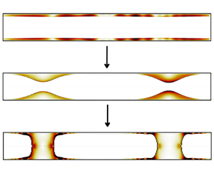
Initial (a,c) and final (b,d) phase distributions inside a capillary caused by the Plateau–Rayleigh instability for $\epsilon =0.1$ (a,b) and $\epsilon =0.2$ (c,d), cf. supplementary movies available at https://doi.org/10.1017/jfm.2024.1024. The lower figures show the channel with the actual aspect ratio.

Although, in a thin film approximation, only collar shapes can be observed (Hammond Reference Hammond1983), Gauglitz & Radke (Reference Gauglitz and Radke1988) developed a lubrication model to capture the collar-plug transition, finding $\epsilon _{cr}\simeq 0.12$. They also compared their predictions to experiments, in which the threshold value was rather $0.09$. They explained this discrepancy by the coalescence of neighbouring collars, that they expect to be responsible of secondary plug formation for $0.09\leq \epsilon <0.12$.

In the present simulations, collars are observed for $\epsilon <0.12$, which agrees with Gauglitz & Radke (Reference Gauglitz and Radke1988). However, secondary coalescence of collars could not be simulated due to mesh resolution limitations when the liquid film between collars thins. When its thickness decreases below 5–10 cells (which eventually occurs for $\epsilon \leq 0.11$) the simulation is considered to be invalid. However, it is possible to observe neighbouring collars getting closer for $\epsilon =0.1$ and 0.11 (figure 4b) that is not yet observed for smaller $\epsilon$. Such a process can eventually lead to their coalescence. Hence, DNS agrees well both with the theory and the experiments of Gauglitz & Radke (Reference Gauglitz and Radke1988). Compared with the Everett & Haynes (Reference Everett and Haynes1972) results, our numerical value is slightly higher than their prediction, which is most probably linked to the existence of satellite lobes between neighbouring collars/plugs. These smaller satellite lobes can retain a significant volume of fluid, which becomes unavailable for the main collar. The static critical thickness is probably underestimating its dynamic value, although the long-term behaviour of static collars is not perfectly accessible in these simulations.

The dynamics of the collar growth was also obtained by Gauglitz & Radke (Reference Gauglitz and Radke1988) with their lubrication model. For the DFT validation, their results (figure 5b) are reproduced using DNS in figure 5(a). The time evolution of the maximum film thickness $h_{max}$ in the central part of the simulation domain is plotted for different $\epsilon$. Because velocities are initialised at zero in DNS, some time is needed to reach a well-established regime. To obtain comparable plots, we choose $t^*=0$ when $h_{max}$ reaches $2h_0$ in figure 5(a). All the curves first exhibit an exponential increase. As experimentally observed by Goldsmith & Mason (Reference Goldsmith and Mason1963), an acceleration occurs next for thick films (in blue) that eventually form plugs. It is due to the cylindrical geometry: for the same change of $h$, the volume that needs to be filled to form a plug is reduced as $h_{max}$ grows. As predicted by Gauglitz & Radke (Reference Gauglitz and Radke1988), this acceleration starts when $h_{max}\simeq 0.6R_0$. These points are indicated by triangles in figure 5. On the contrary, for thin films, the interface decelerates. It then asymptotically reaches the stable collar state of figure 4(b) shown with circle characters. Finally, the films of initial thickness slightly higher than $\epsilon _{cr}$ can first exhibit a deceleration and then an acceleration. Figure 5(a,b) agrees very well, validating the DNS simulations on this particular metric. Notably, collar thickness values are identical for similar cases. The main difference is the behaviour for $\epsilon =0.12\approx \epsilon _{cr}$ where the channel becomes clogged in our DNS but not in the simulations of Gauglitz & Radke (Reference Gauglitz and Radke1988) that were probably not long enough. Similarly, case $\epsilon =0.10$ exhibits a sliding motion at long times, which slightly increases $h_{max}$ .

Figure 5.

Evolution of the maximum film thickness $h_{max}(t)$ for different $\epsilon$. (a) Direct numerical simulation results. (b) Results of Gauglitz & Radke (Reference Gauglitz and Radke1988). Triangles indicate the times where $h_{max}/R_0=0.6$ and circle points indicate particular states with corresponding values of $h_{max}/R_0$. If stable collars are formed, the final value of $h_{max}/R_0$ is indicated. Time scaling $\tilde {t}=t\sigma \epsilon ^3/(3\mu _lR_0)$ follows that of Gauglitz & Radke (Reference Gauglitz and Radke1988).

4.2. Velocity profiles and wall shear stress

Velocity profiles of the channel occlusion phenomenon were obtained both with particle image velocimetry measurements (Bian et al. Reference Bian, Tai, Halpern, Zheng and Grotberg2010), numerically solved analytical models (Johnson et al. Reference Johnson, Kamm, Ho, Shapiro and Pedley1991) and DNS (Tai et al. Reference Tai, Bian, Halpern, Zheng, Filoche and Grotberg2011; Romanò et al. Reference Romanò, Fujioka, Muradoglu and Grotberg2019), thus providing suitable points of comparison. To validate our DNS, we reproduce the results of Tai et al. (Reference Tai, Bian, Halpern, Zheng, Filoche and Grotberg2011) by using the same Laplace number $J_l=0.59$, initial thickness $\epsilon =0.23$, viscosity ratio $m=0.01$ and density ratio $J_g/J_l=0.95$. These parameters only slightly differ from the Bian et al. (Reference Bian, Tai, Halpern, Zheng and Grotberg2010) experimental and Romanò et al. (Reference Romanò, Fujioka, Muradoglu and Grotberg2019) numerical studies concerning the Laplace number. These parameters are used only in this § 4.2, while those of table 1 are used in the rest of the paper.

The velocity fields are presented in figure 6 just before and just after channel occlusion. Before channel occlusion they qualitatively agree with all aforementioned studies. Liquid is driven from the film dips to the collars where the flow is directed towards the tube centre. A motionless zone is observed at the collar centre, close to the wall. The maximum velocity is encountered at the top of a collar. Few instants before channel occlusion, a strong radial acceleration is observed, the maximum velocity being doubled between the two last pictures. Another zone of local maximum velocity is observed at the transition between the main collar and the thin film, close to the interface. It corresponds to the area where the draining process occurs. After channel occlusion, patterns do not change significantly, although a new pivot in the velocity field is obtained at the centre of the symmetry axis. The liquid pushes the plug axially, increasing its width, which was called bifrontal plug growth by Romanò et al. (Reference Romanò, Fujioka, Muradoglu and Grotberg2019). Velocity is maximal just after channel occlusion. They then decrease until a stationary plug state is reached. In this final state, velocity is maximal in the draining zone joining the plug and the film. All these observations were already made by Tai et al. (Reference Tai, Bian, Halpern, Zheng, Filoche and Grotberg2011) before channel occlusion and by Bian et al. (Reference Bian, Tai, Halpern, Zheng and Grotberg2010), Romanò et al. (Reference Romanò, Fujioka, Muradoglu and Grotberg2019) after it.

Figure 6.

Velocity field around channel occlusion time obtained with DNS. The physical parameters are those of Tai et al. (Reference Tai, Bian, Halpern, Zheng, Filoche and Grotberg2011). Velocities are scaled by $\sigma \epsilon ^3/\mu _l$ and time by $\mu _lR_0/\sigma \epsilon ^3$ to conform to Tai et al. (Reference Tai, Bian, Halpern, Zheng, Filoche and Grotberg2011).

A significant difference is however observed here, as an air bubble is produced in the middle of the plug. Formation of secondary bubbles (or droplets in the case of a liquid jet breakup) has already been observed in other experiments such as those by Tjahjadi, Stone & Ottino (Reference Tjahjadi, Stone and Ottino1992). Tjahjadi et al. (Reference Tjahjadi, Stone and Ottino1992) also explained the process of satellite droplet formation and reproduced their own experimental results with the boundary integral method known for its precision of interface description. Similar bubbles were simulated by Newhouse & Pozrikidis (Reference Newhouse and Pozrikidis1992) and Hagedorn, Martys & Douglas (Reference Hagedorn, Martys and Douglas2004). Obtaining a bubble in the middle of a plug is thus normal. One should note that in the Romanò et al. (Reference Romanò, Fujioka, Muradoglu and Grotberg2019) study, VOF simulations were unable to capture small bubbles during collar coalescence, probably because of a too large mesh size; Tai et al. (Reference Tai, Bian, Halpern, Zheng, Filoche and Grotberg2011) could not simulate the plug formation at all.

Velocities are quantitatively in agreement with those of Bian et al. (Reference Bian, Tai, Halpern, Zheng and Grotberg2010), Tai et al. (Reference Tai, Bian, Halpern, Zheng, Filoche and Grotberg2011), Romanò et al. (Reference Romanò, Fujioka, Muradoglu and Grotberg2019). On the contrary, the channel occlusion time differs considerably. Indeed, as already discussed by Tai et al. (Reference Tai, Bian, Halpern, Zheng, Filoche and Grotberg2011), it is not a suitable validation metric, as it strongly depends on the initial conditions (amplitude and velocity), which are not the same in different studies.

In the particular field of lungs airway occlusion, on which previous studies focused (Bian et al. Reference Bian, Tai, Halpern, Zheng and Grotberg2010; Tai et al. Reference Tai, Bian, Halpern, Zheng, Filoche and Grotberg2011; Romanò et al. Reference Romanò, Fujioka, Muradoglu and Grotberg2019), a key parameter is the instantaneous shear stress acting on the channel wall ($\simeq \mu \partial _r v_z$). This parameter is also of significant importance for PEMFC channels, as viscous friction is the main design parameter of channel geometry. The wall shear stress is thus extracted from the previous DNS and plotted in figure 7 at several locations along the tube. Results agree with those of Tai et al. (Reference Tai, Bian, Halpern, Zheng, Filoche and Grotberg2011). After a slow but steady increase, the shear stress explodes a few moments after channel occlusion. It then reduces even more quickly, as observed by Bian et al. (Reference Bian, Tai, Halpern, Zheng and Grotberg2010). All these results confirm that the DFT numerical method used in this paper can be considered as a reference to investigate the Plateau–Rayleigh instability.

Figure 7.

Evolution of the wall shear stress at several locations. Here $z=0$ corresponds to the approximate location of the maximal film thickness. Time is scaled by $\mu _lR_0/\sigma \epsilon ^3$ and the wall shear stress by $\epsilon ^3\sigma /R_0$ to follow Tai et al. (Reference Tai, Bian, Halpern, Zheng, Filoche and Grotberg2011). (a) The DNS results from this study; (b) DNS results from Tai et al. (Reference Tai, Bian, Halpern, Zheng, Filoche and Grotberg2011).

5.1. Governing equations

The previously presented DNS simulations can now be compared with reduced models where inertial and viscous terms can be switched on and off. The present theoretical models use equations and boundary conditions similar to the above numerical approach (cf. § 2). The convective terms $\boldsymbol {v}\boldsymbol {\nabla }\boldsymbol {v}$ are however neglected in the Navier–Stokes equations. Thanks to the axial symmetry, the equations and jump conditions reduce to

(5.1)$$\begin{gather} \frac{\partial v_r}{\partial t} ={-}\frac{1}{\rho} \frac{\partial p}{\partial r} + \nu \left(\frac{\partial^2 v_r}{\partial r^2}+\frac{1}{r}\frac{\partial v_r}{\partial r}-\frac{v_r}{r^2}+\frac{\partial^2 v_r}{\partial z^2}\right), \end{gather}$$

(5.2)$$\begin{gather}\frac{\partial v_z}{\partial t} ={-}\frac{1}{\rho} \frac{\partial p}{\partial z} + \nu \left(\frac{\partial^2 v_z}{\partial r^2}+\frac{1}{r}\frac{\partial v_z}{\partial r}+\frac{\partial^2 v_z}{\partial z^2}\right), \end{gather}$$

(5.3)$$\begin{gather}\frac{\partial v_r}{\partial r} +\frac{v_r}{r}+\frac{\partial v_z}{\partial z}=0, \end{gather}$$

(5.4)$$\begin{gather}{[}\![\boldsymbol{v}]\!]_{r=R_i} = 0, \end{gather}$$

(5.5)$$\begin{gather}{[}\![\boldsymbol{n}\boldsymbol{\cdot}\boldsymbol{\varSigma}]\!]_{r=R_i} = \sigma \kappa\boldsymbol{n}, \end{gather}$$

where $\boldsymbol {\varSigma }$ is the stress tensor and $\nu$ is the kinematic viscosity. The double brackets denote the interfacial jump. A no-slip boundary condition is taken at the wall in $r=R_0$. Finally, the volume conservation in each phase, in the absence of external flow, results in the relationships

(5.6)$$\begin{gather} 2{\rm \pi} R_i v_i =\frac{\partial Q_l}{\partial z} ={-}\frac{\partial Q_g}{\partial z}, \end{gather}$$

(5.7)$$\begin{gather}Q_l+Q_g =0, \end{gather}$$

where $v_i$ is the interfacial velocity.

5.2. Lubrication model with core fluid

To evaluate the influence of inertia on the development of the Plateau–Rayleigh instability, a model without inertia is first developed to be compared with the DNS. The lubrication theory of Gauglitz & Radke (Reference Gauglitz and Radke1988) is extended to consider the core fluid (as it can have significant effects in the plug formation especially when the core radius is small) and a more rigorous account of the cylindrical geometry. The developments are inspired by those of Goyeneche, Lasseux & Bruneau (Reference Goyeneche, Lasseux and Bruneau2002).

The main assumptions for this lubrication model is that the flow is considered laminar and the interface slope is small: $\partial _z h\ll 1$. The interfacial velocity can thus be expressed as

(5.8)\begin{equation} v_i\approx{-}2{\rm \pi} R_i\frac{\partial h}{\partial t} \approx v_r(R_i) . \end{equation}

The magnitude analysis of the continuity equation results in

(5.9)\begin{equation} \frac{v_r}{R_0}\approx\frac{1}{r}\frac{\partial (rv_r)}{\partial r}={-}\frac{\partial v_z}{\partial z}\approx \frac{v_z}{\lambda}. \end{equation}

It is well known that the Plateau–Rayleigh instability does not occur for wavelengths $\lambda$ smaller than $2{\rm \pi} R_i$. Hence, the assumption $\lambda \gg R_i\approx R_0$ is valid, leading to $v_z\gg v_r$. A first limit to the lubrication approximation is obtained here, as for $R_i\ll R_0$, smaller wavelengths can become unstable. With a similar magnitude analysis, the velocity derivatives with respect to $z$ can be neglected compared with those with respect to $r$ and (5.1) and (5.2) reduce to

(5.10)$$\begin{gather} \frac{\partial p}{\partial r} = 0 , \end{gather}$$

(5.11)$$\begin{gather}\frac{\partial p}{\partial z} =\frac{\mu}{r}\frac{\partial}{\partial r}\left(r\frac{\partial v_z}{\partial r}\right). \end{gather}$$

Similarly, the jump conditions at the interface become

(5.12)$$\begin{gather} -[\![p]\!] = \sigma \left(\frac{1}{R_i}+\frac{\partial^2 h}{\partial z^2}\right), \end{gather}$$

(5.13)$$\begin{gather}\left[\!\left[ \mu \dfrac{\partial v_z}{\partial r} \right]\!\right] = 0. \end{gather}$$

These equations, coupled to the no-slip boundary condition lead to the thickness evolution equation (cf. Appendix A)

(5.14)\begin{equation} -2{\rm \pi} R_i\frac{\partial h}{\partial t}= \sigma\frac{\partial}{\partial z} \left[ \beta \left( \frac{\partial^3 h}{\partial z^3}+\frac{1}{R_i^2}\frac{\partial h}{\partial z}\right) \right],\end{equation}

where

(5.15)\begin{equation} \beta={-}\dfrac{{\rm \pi} R_i^4}{8\mu_l}\left\{ \dfrac{( R_0^2-R_i^2)[ 4m(R_0^2-R_i^2)+(3R_i^2-R_0^2)] }{mR_0^4+(1-m)R_i^4} +4\ln\left(\frac{R_i}{R_0}\right) \right\}. \end{equation}

Equation (5.14) is both analysed in the linear regime (§ 6) and numerically solved outside (§ 7). In the linear regime, where the film thickness writes

(5.16)\begin{equation} h(z,t)=h_0+A_0\exp({\rm i}\omega t+{\rm i}kz),\end{equation}

(5.14) results in the following dimensionless dispersion relation:

(5.17)\begin{equation} \hat{\omega}=x^2(x^2-1)\hat{\beta}.\end{equation}

Here $\hat {\beta }=\beta \mu _l/(2{\rm \pi} R_i^4)$ and $x=kR_i$ is a dimensionless wavenumber. This number is real, as well as the instability increment (growth rate) $\omega _i=-{\rm i}\omega$. The dimensionless growth rate is defined as $\hat {\omega }=\omega _i\mu _lR_i/\sigma$.

5.3. Linear stability models accounting for viscosity and inertia

5.3.1. Previous results

As our starting point, we need to mention several previous results. First, Tomotika (Reference Tomotika1935), following Rayleigh (Reference Rayleigh1878), proposed a general theory considering both viscosity and inertia for both fluids for the case of the fluid jet ($R_0\to \infty$). Tomotika investigated the cases where viscosity dominates and where the viscosity ratio is neither zero nor infinite. Tomotika proposed to write the dispersion relation compactly as a matrix ${\boldsymbol{\mathsf{M}}}$, the determinant of which is zero. In the present notation, Tomotika's matrix writes

(5.18) \begin{align} {\boldsymbol{\mathsf{M}}}=\begin{bmatrix} I_1(x) & I_1(x_g) & K_1(x) & K_1(x_l) \\ xI_0(x) & x_gI_0(x_g) & -xK_0(x) & -x_lK_0(x_l) \\ 2mx^2 I_1(x) & m(x^2+x_g^2)I_1(x_g) & 2x^2K_1(x) & (x^2+x_l^2)K_1(x_l) \\ F_1 & F_2 & 2x^2K'_1(x)+\hat{\omega}J_lK_0(x) & 2xx_lK'_1(x_l) \end{bmatrix},\end{align}

with

(5.19)$$\begin{gather} F_1=2mx^2 I'_1(x)-\hat{\omega}J_gI_0(x)+x\frac{x^2-1}{\hat{\omega}}I_0(x), \end{gather}$$

(5.20)$$\begin{gather}F_2=2mxx_g I'_1(x_g)+x\frac{x^2-1}{\hat{\omega}}I_0(x_g). \end{gather}$$

Here, $I_i$ and $K_i$ are the $i$th order modified Bessel functions of the first and second kind, respectively. The prime denotes a derivative. Here $x_g$ and $x_l$ are related to $x$ by

(5.21a,b)\begin{equation} x_g^2=x^2-\hat{\omega}J_g, \quad x_l^2=x^2-\hat{\omega}J_l. \end{equation}

In parallel to these liquid/gas jet studies, Goren (Reference Goren1962) studied the effect of confinement (finite $R_0$) by neglecting the core fluid. Goren obtained a $4\times 4$ matrix with different coefficients.

Finally, Georgiou et al. (Reference Georgiou, Papageorgiou, Maldarelli and Rumschitzki1991) gathered all these models to consider both the core and outer fluids for finite $R_0$. Hence, they had to solve the determinant of a $6\times 6$ matrix. However, as their objective was to analyse the impact of electric properties of fluids with similar densities (the outer liquid was an electrolyte and the core, a dielectric fluid) they used a single density and Laplace number for the core and outer fluids.

5.3.2. Present model

In the present study, as the densities of water vapour and liquid water are several orders of magnitude different, the Georgiou et al. (Reference Georgiou, Papageorgiou, Maldarelli and Rumschitzki1991) model will be generalised for two different fluid densities. We describe here briefly how the dispersion relation is derived and present its final formulation. A more detailed derivation is proposed in Appendix B.

In order to automatically verify the continuity equation (5.3), the radial and axial velocities are expressed with the streamfunction $\psi$,

(5.22a,b)\begin{equation} v_r=\frac{1}{r}\frac{\partial \psi}{\partial z} \quad \text{and} \quad v_z={-}\frac{1}{r}\frac{\partial \psi}{\partial r}.\end{equation}

Here $v_r$ and $v_z$ are then substituted in the Navier–Stokes equations (5.1) and (5.2) and the pressure terms are eliminated, leading to

(5.23)\begin{equation} \left(D-\frac{1}{\nu}\frac{\partial}{\partial t}\right)D\psi=0, \end{equation}

where the differential operator $D={\partial ^2}/{\partial r^2}-({1}/{r})({\partial }/{\partial r})+{\partial ^2}/{\partial z^2}$.

It should be noted that in the current linear stability analysis, the convective terms are automatically negligible as they evolve quadratically with the perturbation and are exactly zero for the chosen primary flow.

As $D$ and $(D-\nu ^{-1}\partial _t )$ are commutative, when $\nu ^{-1}\neq 0$, $\psi$ can be written as a linear combination of $\psi _1$ and $\psi _2$ where

(5.24a,b)\begin{equation} D\psi_1=0 \quad \text{and} \quad \left(D-\frac{1}{\nu}\frac{\partial}{\partial t}\right)\psi_2=0. \end{equation}

Expressing $\psi _j (j=1,2)$ as $\psi _j=\phi _j \exp ({\rm i}\omega t+{\rm i}kz)$, $\phi _j$ are solutions of

(5.25)\begin{equation} \frac{{\rm d}^2 \phi_j}{{\rm d}r^2}-\frac{1}{r}\frac{{\rm d}\phi_j}{{\rm d}r}-k_j^2\phi_j=0, \end{equation}

with $k_1=k$ and $k_2^2=k^2+{\rm i}\omega /\nu$. The solutions of (5.25) are linear combinations of $I_1(k_jr)$ and $K_1(k_jr)$. In each fluid, the streamfunction can then be written as a linear combination of four terms, one for each $k_j$ and for each kind of modified Bessel function ($I_1$ and $K_1$). Hence, eight constants are needed to completely define the velocity profile, four in each fluid. This number is reduced to six, as the velocity must be finite in $r=0$, requiring the $K_1$ constants in the core fluid to be zero.

The no-slip boundary condition (two equations) and the velocity continuity at the interface (5.4) (two equations) first give four equations. The continuity of the tangential and normal stresses ((5.5) projected to the tangential and normal directions) write in the small-slope approximation

(5.26) $$\begin{gather} \left[\!\left[ \mu\left(\dfrac{\partial v_z}{\partial r}+\dfrac{\partial v_r}{\partial z}\right)\right]\!\right]_{r=R_i}=0 , \end{gather}$$

(5.27) $$\begin{gather}\left[\!\left[ -p + 2\mu\dfrac{\partial v_r}{\partial r}\right]\!\right]_{r=R_i}= \sigma\left(\frac{1}{R_i}+\frac{\partial^2 h}{\partial^2 z}\right) . \end{gather}$$

Equation (5.26) leads to the fifth equation. Finally, combining (5.27) with (5.2), (5.6) and (5.7), leads to the last equation

(5.28) \begin{equation} \left[\!\left[ -{\rm i}\omega\dfrac{\rho}{r}\dfrac{\partial \psi}{\partial r}+\dfrac{\mu}{r}\dfrac{\partial}{\partial r}D\psi +2{\rm i}k\mu\dfrac{\partial v_r}{\partial r} \right]\!\right]=\frac{k}{\omega}\sigma\frac{( kR_i)^2-1}{R_i^2}v_r.\end{equation}

The set of six equations with six unknowns is homogeneous (Appendix B). Their matrix can be rearranged as

(5.29) \begin{align} \small{ {\boldsymbol{\mathsf{M}}}=\begin{bmatrix} 0 & 0 & K_1(ax) & K_1(ax_l) & I_1(ax) & I_1(ax_l) \\ 0 & 0 & -K_0(ax) & -\dfrac{x_l}{x} K_0(ax_l) & I_0(ax) & \dfrac{x_l}{x} I_0(ax_l) \\ I_1(x) & I_1(x_g) & -K_1(x) & -K_1(x_l) & -I_1(x) & -I_1(x_l) \\ I_0(x) & \dfrac{x_g}{x}I_0(x_g) & K_0(x) & \dfrac{x_l}{x} K_0(x_l) & -I_0(x) & -\dfrac{x_l}{x}I_0(x_l) \\ (m-1) I_1(x) & \left[ (m-1)-\dfrac{\hat{\omega}J_g}{2x^2}\right] I_1(x_g) & 0 & \dfrac{\hat{\omega}J_l}{2x^2} K_1(x_l) & 0 & \dfrac{\hat{\omega}J_l}{2x^2}I_1(x_l) \\ F'_1 & F'_2 & \hat{\omega}J_lK_0(x) & 0 & -\hat{\omega}J_lI_0(x) & 0 \end{bmatrix}},\end{align}

with

(5.30)$$\begin{gather} F'_1 =2(1-m)x^2 I'_1(x)+\hat{\omega}J_gI_0(x)+x\frac{x^2-1}{\hat{\omega}}I_1(x), \end{gather}$$

(5.31)$$\begin{gather}F'_2 = 2(1-m) x_gx I'_1(x_g)+x\frac{x^2-1}{\hat{\omega}}I_1(x_g). \end{gather}$$

Here, $x_{l,g}=k_{l,g}R_i$ are defined by (5.21a,b); $a=R_0/R_i=(1-\epsilon )^{-1}$ is the radius ratio. We remind that the dispersion relation reads $\det {\boldsymbol{\mathsf{M}}}=0$.

In the limit $R_0\to \infty$, the first two rows and the last two columns can be dropped from ${\boldsymbol{\mathsf{M}}}$ so the velocities do not diverge at $r\to \infty$. The Tomotika (Reference Tomotika1935) matrix (5.18) is thus found (with some rearrangements). Similarly, if the core gas is forgotten, the first two columns (representing the core fluid) and the third and fourth row (velocity continuity) are dropped leading to the matrix of Goren (Reference Goren1962). Finally, if both fluids have the same densities ($J_l=J_g$), the case of Georgiou et al. (Reference Georgiou, Papageorgiou, Maldarelli and Rumschitzki1991) without electromagnetic effects is found. Model (5.29) is called the ‘visco-inertial linear model’ hereafter, as it is designed for linear stability studies and accounts for both viscous and inertial terms.

5.3.3. Absence of inertia

In the case where inertia is neglected, $J_l,J_g\to 0$ and $\det {\boldsymbol{\mathsf{M}}}$ is trivially zero, as the columns of (5.29) are equal two by two as $x_l=x_g=x$. This comes from the simplification of (5.23) to $D^2\psi =0$. To solve this issue, $\psi _2$ must be modified to be linearly independent of $\psi _1$, which is not modified and still verifies $D\psi _1$. Hence, $\psi _2$ is now a solution of $D\psi _2=\psi _1$. Therefore, $\psi _2$ is a linear combination of $r^2I_0(kr)$ and $r^2K_0(kr)$. The velocity expressions detailed in Appendix B are modified accordingly. Using the same boundary conditions, the matrix ${\boldsymbol{\mathsf{M}}}$ is modified and rearranged as

(5.32) \begin{align} {\boldsymbol{\mathsf{M}}}=\begin{bmatrix} 0 & 0 & K_1(ax) & axK_0(ax) & I_1(ax) & axI_0(ax) \\ 0 & 0 & -K_0(ax) & f_k(ax) & I_0(ax) & f_i(ax) \\ I_1(x) & xI_0(x) & -K_1(x) & -xK_0(x) & -I_1(x) & -xI_0(x) \\ I_0(x) & f_i(x) & K_0(x) & -f_k(x) & -I_0(x) & -f_i(x) \\ (m-1) I_1(x) &\begin{array}{@{}l@{}} mI_1(x)+(m-1)\\ \quad\times\, xI_0(x)\end{array} & 0 & K_1(x) & 0 & -I_1(x) \\ G'_1 & G'_2 & K_1(x) & 0 & I_1(x) & 0 \end{bmatrix},\end{align}

with

(5.33)$$\begin{gather} f_k(x) =2K_0(x)-xK_1(x), \end{gather}$$

(5.34)$$\begin{gather}f_i(x) = 2I_0(x)+xI_1(x), \end{gather}$$

(5.35)$$\begin{gather}G'_1 =(1-m)xI_0(x)+(m-2)I_1(x)+\frac{x^2-1}{2\hat{\omega}}I_1(x), \end{gather}$$

(5.36)$$\begin{gather}G'_2 = (1-m) x^2I_1(x)+x\frac{x^2-1}{2\hat{\omega}}I_0(x). \end{gather}$$

As in Tomotika (Reference Tomotika1935), this matrix can also be obtained by letting $J_l,J_g\to 0$ in (5.29). Unlike the lubrication theory, our model does not assume the axial and radial velocities to be independent. All terms of the viscous contribution to the Navier–Stokes equations (5.1) and (5.2) are considered. Model (5.32) is subsequently referred to as the ‘viscosity-only linear model’.

5.3.4. Absence of viscosity

In the absence of viscosity, the Navier–Stokes equations reduce to those of Euler. Hence, $\psi$ now verifies $D\psi =0$, leading to $\psi =\psi _1$ only. Hence, the second, fourth and sixth columns in (5.29) disappear. Moreover, the absence of viscosity removes the tangential no-slip wall condition and the tangential stress and velocity continuity conditions at the interface. The second, fourth and fifth rows disappear and (5.29) simplifies to

(5.37)\begin{equation} {\boldsymbol{\mathsf{M}}}=\begin{bmatrix} 0 & K_1(ax) & I_1(ax)\\ I_1(x) & -K_1(x) & -I_1(x) \\ F'_1 & \hat{\omega}J_lK_0(x) & -\hat{\omega}J_lI_0(x) \end{bmatrix},\end{equation}

with $F'_1 = x(({x^2-1})/{\hat {\omega }})I_1(x)+\hat {\omega }J_gI_0(x)$. Note that, although $\mu _l$ is present in the scaling of both $J_{l,g}$ and $\hat {\omega }$, it cancels out of the dispersion relation. Model (5.37) is subsequently referred to as the ‘inertia-only linear model’.

6.1. Influence of the core fluid

While most thin film models in microscopic tubes consider only the outer fluid (Goren Reference Goren1962; Hammond Reference Hammond1983; Frenkel et al. Reference Frenkel, Babchin, Levich, Shlang and Sivashinsky1987; Gauglitz & Radke Reference Gauglitz and Radke1988; Johnson et al. Reference Johnson, Kamm, Ho, Shapiro and Pedley1991; Eggers & Dupont Reference Eggers and Dupont1994; Lister et al. Reference Lister, Rallison, King, Cummings and Jensen2006a), some authors include the effect of the core, which substantially complicates the theory (Georgiou et al. Reference Georgiou, Papageorgiou, Maldarelli and Rumschitzki1991; Halpern & Grotberg Reference Halpern and Grotberg2003; Dietze & Ruyer-Quil Reference Dietze and Ruyer-Quil2015; Camassa et al. Reference Camassa, Ogrosky and Olander2017). Nevertheless, a quantitative evaluation of the core flow effect appears relevant when analysing plug formation, especially to later investigate the conditions under which the Plateau–Rayleigh instability can be saturated by an imposed core gas flow. In this section we thus analyse the influence of the core fluid on the linear stability in two steps. First the analysis will be restricted to the viscous problem modelled by the viscosity-only linear model (5.32) and by the lubrication dispersion relationship (5.17). Then a similar analysis will be performed on the inertial problem modelled by the inertia-only linear model (5.37).

Figure 8 presents the results of several simulations for various values of $m$ and $h_0$ and for both the lubrication with the core fluid model and the viscous linear one. In order to obtain similar orders of magnitude for different $\epsilon$, and thus, to better observe the differences due to the viscosity ratio, the growth rates are scaled by $\epsilon ^3/3$. Indeed, in the thin film limit, a Taylor expansion of (5.17) at leading order in terms of the dimensionless film thickness $\epsilon =h_0/R_0$ results in

(6.1)\begin{equation} \hat{\omega}=\frac{\epsilon^3}{3} (x^2-x^4).\end{equation}

Figure 8.

Impact of the viscosity ratio $m$ on the convergence of the growth rate to the thin film approximation. Different colours indicate the average film thickness $\epsilon$. Results are shown for (a) $m=0$, inviscid core fluid; (b) $m=1$, equal viscosities of core and outer fluids; (c) $m=10$, more viscous core fluid; (d) $m=0.0438$ corresponding to the water parameters of table 1. Solid lines: thin film lubrication model (6.1). Dash-dotted lines: viscosity-only model (5.32). Dotted lines: lubrication model (5.17).

Figure 8 shows that, whatever the viscosity ratio is, the curves converge towards the classical thin film lubrication approximation (6.1) (plotted with a solid line) when $\epsilon \to 0$. However, this convergence is much quicker for the particular case of fluids with equal viscosities (figure 8b). Indeed, the Taylor expansion of (5.17) can be pursued at the next order with respect to $\epsilon$ giving

(6.2)\begin{equation} \hat{\omega}=\frac{\epsilon^3}{3} (1+3(1-m)\epsilon)(x^2-x^4).\end{equation}

The second-order term disappears for $m=1$. This explains the observation of Georgiou et al. (Reference Georgiou, Papageorgiou, Maldarelli and Rumschitzki1991) that the agreement between their model and the classical lubrication (6.1) is ‘exceptional even for $\epsilon$ as large as 0.2’. Moreover, in the other cases, (6.2) proves that the instability is accelerated for thicker films if $m<1$ (the core fluid is less viscous than the outer one; see first and last plots). On the contrary, if the core fluid is more viscous (figure 8c), the instability slows down for thick films.

Such observations stress the importance of the core fluid effect. Indeed, compared with the case without core fluid (figure 8a), the growth rate is reduced in the practically important water case (figure 8d). The core gas slightly slows down the instability in thick films.

Finally, the lubrication model with core fluid (5.17) appears to agree with the viscosity-only linear model (5.32) where all viscous contributions to the Navier–Stokes equations are considered. The agreement is perfect for thin films or highly viscous core fluids but is still reasonable for thicker films and less viscous core fluids. This validates the use of the lubrication with the core fluid model (5.14) to predict the nonlinear evolution of the system in the absence of inertia (see § 7.2).

Concerning the inertial contribution of the core fluid, it is a priori expected to be negligible as the Laplace number $J_g$ of the core fluid is two orders of magnitude smaller than that of the liquid film $J_l$. However, the effect of the density ratio for other fluids can be studied. When considering the inertia-only problem (5.37), the lubrication reference curve becomes irrelevant and must be modified by the thin film limit

(6.3)\begin{equation} \hat{\omega}=x\sqrt{1-x^2}\frac{\sqrt{\epsilon}}{\sqrt{J_l}}\end{equation}

of the inertia-only model (5.37). Figure 9 provides the dispersion curves that come from (5.37) for several density ratios $J_g/J_l$. The reference curve in black is (6.3). To obtain results with similar magnitudes, the growth rates are scaled by $\sqrt {\epsilon /J_l}$.

Figure 9.

Impact of the density ratio $J_g/J_l$ on the growth rate. Different colours indicate the average film thickness $\epsilon$. Results are shown for (a) $J_g=0$, no core fluid; (b) $J_g=J_l$, equal densities of core and outer fluids; (c) $J_g=10J_l$, denser core fluid; (d) $J_g=6.23\times 10^{-4} J_l$ corresponding to the water parameters of table 1. Solid lines: inertia-only thin film model (6.3). Dash-dotted lines: inertia-only linear model (5.37).

Similarly to the above viscosity-only analysis, growth rates for the inertia-only model (5.37) tend towards the thin film limit (6.3) when $\epsilon \to 0$ whatever the density ratio is. Moreover, an increase in the core fluid density results in a decreasing growth rate, meaning the Plateau–Rayleigh instability slows down. Indeed, the denser the core fluid, the more difficult it is to displace. The fastest convergence to the thin film approximation is found for an intermediate density ratio $J_g/J_l=3/4$ (this can be obtained by pursuing the Taylor expansion of (5.37) at the next order in $\epsilon$). Finally, as in the above viscosity-only case, no clear difference between the real case scenario of figure 9(d) and the coreless scenario of figure 9(a) can be noticed. As expected, the inertial contribution of the core gas can thus be safely neglected.

6.2. Transition between viscous and inertial regimes

We now consider the practical case of water (table 1) that corresponds to $m=4.38\times 10^{-2}$, $J_l=3.6\times 10^5( 1-\epsilon )$ and $J_g=224.3( 1-\epsilon )$. With these parameters, the viscosity-only, inertia-only and visco-inertial linear stability models (5.32), (5.37) and (5.29) are solved and compared in figure 10 for different $\epsilon$ values. As in figure 8, growth rates are scaled by $\epsilon ^3/3$.

Figure 10.

Comparison of the effects of inertia and viscosity on the growth rate. (a–c) Dispersion curves for the three linear stability models: (a) viscosity-only model, (b) inertia-only model, (c) visco-inertial model. Different colours indicate the average film thickness $\epsilon$. Dash-dotted lines: linear stability model. Solid lines on all graphs: thin film lubrication approximation (6.1). Triangle characters on all graphs: growth rates extracted from DNS. (d) Maximum growth rate as a function of $\epsilon$. All curves are from linear stability models, either viscosity-only (long red dashes), inertia-only (green dashes) or visco-inertial (yellow solid line).

Direct numerical simulations are also performed for different initial perturbation wavelengths to find the growth rates in the linear regime. Their determination is discussed in Appendix C. The obtained growth rate is plotted as a function of the wavenumber with triangle characters in figure 10. Due to the incoherence of initial conditions in DNS and in the theory (cf. Appendix C), the exponential growth stage does not start at $t=0$ and should thus be identified. This causes uncertainties illustrated with error bars. During this process, it is particularly important to ensure that the measured growth rate is associated to the correct wavelength. Indeed, the final wavelength of the perturbation can be different from the initial one as it is always shifted towards that of the maximal growth rate. Direct numerical simulations include all the relevant phenomena: viscosity, capillarity, convection and inertia.

The viscosity-only model (5.32) agrees with DNS for thin films ($\epsilon \leq 0.1$), cf. figure 10(a). Small discrepancies appear only close to the maximum growth rate. However, significant differences occur for thicker films. While the viscosity-only model results in a positive deviation from the thin film lubrication approximation, the growth rate of the instability is actually lower.

On the contrary, the inertia-only model (5.37) agrees with DNS for thick films $\epsilon \geq 0.3$ (cf. figure 10b) while the model strongly differs at small $\epsilon$. This clearly indicates a transition from a viscous regime for $\epsilon \leq 0.1$ to an inertial regime for $\epsilon \geq 0.3$. In the overall picture, both terms are essential to capture the instability inception. This is apparent in figure 10(c) where DNS is compared with the visco-inertial linear model (5.29). Here, the agreement is of high quality whatever the average film thickness.

Since the visco-inertial linear model agrees with DNS, it can be used to obtain the maximum growth rate for several thicknesses. The results are plotted in figure 10(d) and are compared with the inertia-only and viscosity-only linear models. The cross-over between these regimes is clear here: while for $\epsilon \lesssim 0.1$, the maximum growth rate follows the viscosity-only curve, it corresponds to the inertia-only model for $\epsilon \gtrsim 0.25$. In the transition zone $0.1\leq \epsilon \leq 0.25$, both viscosity and inertia are important.

The inertial regime validity for thick films shows that the core vapour can be neglected in the water vapour/liquid water system. Indeed, with the physical parameters of table 1, the core gas effect was observed only for thick films in the viscosity-only model of figure 8. However, as demonstrated above, these films actually follow the inertial regime where the core gas does not affect the growth rates (figure 9). Hence, the core gas has almost no influence on the linear regime of the Plateau–Rayleigh instability. Such a conclusion can be verified with the visco-inertial linear model, within which the curves with or without the core gas perfectly overlap (this was verified by the authors).

Finally, a significant outcome of figure 10(b) is that, for the chosen physical system, the prediction of the inertial linear model is higher than that of the thin film lubrication for thin films and lower for thick films. Indeed, in the absence of viscosity, the growth rate vanishes for $\epsilon \to 1$ while it takes a finite value in the thin film approximation, meaning that the ratio diverges accounting for the $\epsilon ^3$ lubrication scaling. The $\epsilon ^3$ scaling is replaced in that case by the $\sqrt {\epsilon }$ scaling of (6.3).

In the present paper a no-slip condition has been imposed at the wall. This choice is reasonable for the millimetric film-covered channels studied here, although at small scale this condition can break down. Zhao, Zhang & Si (Reference Zhao, Zhang and Si2023) studied the effects of slip on the linear stability of Plateau–Rayleigh instability and demonstrated that it speeds up its development, notably for thin films and micrometric channels. This enhancement of the instability equally affects the nonlinear regime, for example, by accelerating the film thinning (Liao, Li & Wei Reference Liao, Li and Wei2013), which may modify the critical thickness separating stable collars and plugs due to volume retention in satellite lobes as discussed later in §§ 7.2 and 7.3. Slip is finally expected to increase the wavelength of maximum instability (Zhao et al. Reference Zhao, Zhang and Si2023).

In this section a transition between an inertial and a viscous regime has been discussed for small perturbations. In the next section the underlying mechanisms of this transition will be studied by enlarging the previous temporal study to observe spatial dependencies of viscous and inertial contributions, both in the linear and nonlinear regimes.

7.1. Comparative analysis of forces in the linear regime

We first confirm and refine the previous linear regime results. Figure 11 presents a map of the magnitudes of the three aforementioned contributions in the linear regime of DNS, for a mostly viscous case ($\epsilon =0.1$) and a transitional visco-inertial case ($\epsilon =0.2$). The colour scales differ between figures to show the spatial variation of each term. The simulation times have been chosen arbitrarily within the regime of exponential growth. Results have been checked at twice these times and give very similar results with slightly higher magnitudes.

Figure 11.

Spatial dependence of the contribution of viscosity (a,d), inertia (b,e) and convection (c,f) in the linear regime obtained by DNS. Data for $\epsilon =0.1$ at $t=10$ ms are shown in (a–c), while those for $\epsilon =0.2$ at $t=5$ ms are presented in (d–f). Note the different colour scale for different subfigures.

First, one can confirm that convection can be neglected in the above linear models. Its contribution is at least one order of magnitude smaller than those of inertia and viscosity. Moreover, all contributions are negligible in the core flow, thus supporting results from § 6. In the thin film case $\epsilon =0.1$, as expected, the viscous contribution largely dominates that of inertia, being one order of magnitude higher. When $\epsilon =0.2$, inertia and viscosity terms are comparable in agreement with the previous discussion. Inertia is slightly more important, being resent within a larger domain of the liquid.

A clear spatial separation between inertia and viscosity is also observed, the former acting mostly near the interface while the latter is maximal close to the wall. Such a separation is present at any time in all simulations, in both linear and nonlinear regimes. From an energy point of view, the energy can only come from surface tension forces acting at the interface. This energy is converted into kinetic energy, then transported to the wall and finally dissipated there by viscosity. In the thin film case, the main kinetic transport contribution seems to be the viscous diffusion, which does not depend on $r$ and is everywhere higher than inertia. In the thick film case, however, kinetic energy is transported mostly by inertial forces; the viscous diffusion is much smaller at the interface. In practice, the transition between the viscous and the inertial regime is a transition between a diffusive and a direct inertial transport process of kinetic energy. The inertia, viscous and convection terms are maximal at the collar edges and minimal inside them. The dynamics is thus mostly driven by what happens at the collar edges.

7.2. Nonlinear formation of satellite lobes

Extensive studies of the long-term behaviour of thin films were previously carried out, notably by Hammond (Reference Hammond1983) and Lister et al. (Reference Lister, Rallison, King, Cummings and Jensen2006a). Based on a simple lubrication model, Hammond (Reference Hammond1983) studied the formation and evolution of satellite lobes that appear between the main collars. Hammond (Reference Hammond1983) simulations were restricted to domains where main collars cannot move. Lister et al. (Reference Lister, Rallison, King, Cummings and Jensen2006a) extended this study and discovered that main collars and satellite lobes can exhibit a sliding motion. In both studies, only viscous lubrication models were used, which underlines the crucial role of viscosity in long-term thin film dynamics. Satellite lobe formation is explained by the interplay of several effects. Initially, the film dips as they have a larger interface radius present a higher capillary pressure. Liquid is thus drained from dips to collars, which is the primary instability mechanism. It is only valid for long wavelengths where the axial curvature $\partial _{zz}h$ is smaller than the radial one. However, as the film thins, viscous forces become significant, slowing down the drainage process. Viscous forces, at first order, are proportional to $h^{-3}$. Hence, they are bigger at the dip centre than on the main collar edges. As a consequence, the dip flattens. In a flat film portion the pressure gradients vanish, thus stopping the drainage. However, the flow persists close to collars where the film slope is non-zero. This creates new local minima and satellite lobes. These lobes have a smaller axial extent and are stable against the Plateau–Rayleigh mechanism as their axial curvature dominates their radial one, explaining why they are finally drained into the main collars. A similar mechanism is also observed in the Rayleigh–Taylor instability (Lister, Rallison & Rees Reference Lister, Rallison and Rees2006b), which is well described in Dietze, Picardo & Narayanan (Reference Dietze, Picardo and Narayanan2018, figure 2).

These lobes are observed in our DNS, cf. figure 4(b) (slightly visible e.g. at $z=0.35L$) and figure 12. They can be equally obtained by solving numerically the lubrication equation (5.14). Figure 13(a) illustrates one time step soon after the satellite lobes formation obtained with (5.14). The ability of the lubrication approximation to recover DNS results confirms that satellite lobe formation is only driven by viscous and capillary forces but not by inertia. This result was already present in the fact that Lister et al. (Reference Lister, Rallison, King, Cummings and Jensen2006a); Dietze et al. (Reference Dietze, Picardo and Narayanan2018) found similar results, although the latter model included the inertial and convective terms while the former considered only the viscosity contribution. Figure 12(a–c) demonstrates that viscous terms are several orders of magnitude larger than those of inertia and convection during the satellite lobe development. We note that the viscous forces on the wall evolve nearly linearly with time, while both inertia and convection diminish over time; the film evolution becomes quasi-static.

Figure 12.

Spatial dependence of the contribution of viscosity (a,d), inertia (b,e) and convection (c,f) at satellite lobe formation obtained by DNS. Data for $\epsilon =0.1$ at $t=100$ ms are shown in (a–c), while those at $t=300$ ms are presented in (d–f). Note the different colour scale for different subfigures.

Figure 13.

Interface shapes obtained with lubrication equation (5.14) for the same parameters as figure 12.

At large time scales, as expected by Lister et al. (Reference Lister, Rallison, King, Cummings and Jensen2006a), Dietze & Ruyer-Quil (Reference Dietze and Ruyer-Quil2015), Dietze et al. (Reference Dietze, Picardo and Narayanan2018), collars start sliding. We observe such an effect both in DNS and lubrication results, although not identically. In DNS the collars direct themselves to the domain centre, while within the lubrication approach (figure 13b), they get closer two by two. One probable explanation for this is that lateral boundary conditions are not exactly identical in DNS and lubrication simulations. Finally, lobes and collars can collide and either merge (thus creating bigger collars or even plugs) or rebound without merging, as expected by Lister et al. (Reference Lister, Rallison, King, Cummings and Jensen2006a). It is not possible to know which of these two scenarios will occur as DNS results become uncertain when the film thins too much. Indeed, DNS results should be assumed valid only when at least 10 mesh cells are present in the film. An adaptive mesh would solve this problem but is not yet implemented. Overall, even during the sliding motion, inertial and convective contributions are negligible compared with viscous forces, as observed in figure 12 just before ($t=100$ ms) and during ($t=300$ ms) sliding.

7.3. Nonlinear plug formation

In this section we examine the nonlinear channel occlusion phenomenon that occurs for thick films.

7.3.1. Plug formation time

As the lubrication equation has proven to be invalid in the linear regime, it cannot be used for this case. We first consider the occlusion times for a given $\epsilon$. Assuming the linear regime during all the evolution (which is, of course, untrue), the occlusion time is expected to be defined by the growth rate $\omega _i$ as

(7.1)\begin{equation} t_{plug}^{lin}=\ln \left[\frac{(1-\epsilon)R_0}{A_0}\right]\frac{1}{\omega_i},\end{equation}

where $A_0$ is the amplitude of the initial perturbation and $(1-\epsilon )R_0=R_i$ is the initial core vapour radius. It corresponds to the radius to fill to close the channel. Figure 14 compares the value of (7.1) and $t_{plug}$ observed in DNS. For thick films ($\epsilon \geq 0.14$), $t_{plug}^{lin}\propto t_{plug}$ and the occlusion time is regularly overestimated by (7.1). It indicates that the behaviour in the nonlinear regime is probably similar to the linear regime, but that it is accelerated close to the tube centre. However, this observation does not stand for films of thickness just above $\epsilon _{cr}$, where the occlusion is strongly delayed ($t_{plug}\gg t_{plug}^{lin}$) as already observed in figure 5. Dietze & Ruyer-Quil (Reference Dietze and Ruyer-Quil2015) have explained this delay by a ‘viscous-blocking’ mechanism where the viscous dissipation slows down the instability and allows the formation of satellite lobes between primary collars (which is discussed in the previous section for thin films). The liquid volume available for plugs is thus reduced and occlusion is not observed. It may explain the discrepancy between the critical volume obtained on the one hand by Gauglitz & Radke (Reference Gauglitz and Radke1988) and by us, cf. § 4.1 and on the other hand by Everett & Haynes (Reference Everett and Haynes1972).

Figure 14.

Dimensionless occlusion time observed in DNS compared with the dimensionless occlusion time predicted from the linear regime via (7.1). Time is scaled by $\mu _lR_0/\sigma \epsilon ^3$. The solid orange line is a linear fit to the points with $\epsilon >0.15$. Its slope is $0.86$ with a regression coefficient $0.99989$. The dashed black line is $t^*_{plug}=t^{*lin}_{plug}$.

Figure 15 evaluates the different contributions to the pressure gradient for the case $\epsilon =0.2$ at three stages: well before the channel occlusion, immediately before and after. Long before channel occlusion, as in the linear regime, viscous and inertial forces have similar orders of magnitude while being spatially separated. Nevertheless, convection becomes significant, though still smaller than other contributions. As expected, this regime is similar to the linear regime.

Figure 15.

Spatial dependence of the contribution of viscosity (a,d), inertia (b,e) and convection (c,f) in the linear regime obtained by DNS. Data for $\epsilon =0.2$ at $t=18$ ms are shown in (a–c), those at $t=19$ ms are in (d–f) and those at $t=20$ ms are presented in (g–h). Note the different colour scale for different subfigures.

Just before the channel occlusion, a strong increase of inertial and convective contributions is observed at the top of the rising collar. This increase agrees with Gauglitz & Radke (Reference Gauglitz and Radke1988) who mentioned that a clear acceleration in the rising process is observed when the film reaches a thickness of $0.6R_0$, cf. figure 5. Such high values of inertia and convection in the tip of the collar is due to the cylindrical geometry: as the collar rises, it has a smaller space to fill, while still accelerating due to the exponential behaviour of the Plateau–Rayleigh instability. This phenomenon appears very briefly (here during approximately 1 $\mathrm {\mu }$m), explaining why $t_{plug}^{lin}$ approximates well $t_{plug}$.

Such a concentration of inertia and convection at the tip of the rising collar seems to point towards a transition between a regime where inertia/convection and viscous forces are both significant but spatially separated and a regime where the collar growth is only governed by inertial and convective contributions. To confirm this analysis, the evolution of the core gas throat radius $R_{min}=R_0-h_{max}$ is plotted against the time remaining before plug formation $t_{plug}-t$ in figure 16. A log-log scale is used to identify the relevant power laws. For the breakup of liquid jets, Eggers & Villermaux (Reference Eggers and Villermaux2008) identified three scaling laws $R_{min}\propto (t_{plug}-t)^\alpha$. First, when inertia and surface tension effects are balanced, the dimensional analysis predicts $\alpha =2/3$. If viscous terms and surface tension are balanced, $\alpha \approx 0.175$. Finally, in the case where all three contributions are important, $\alpha =1/2$. Although these laws were derived for the case where only the inner fluid is considered, it is reasonable to assume that they are still relevant for the outer fluid case. However, one mentions that the inner fluid should play a significant role when $R_{min}$ becomes sufficiently small. As $R_{min}$ decreases, it appears to follow a time scaling with increasing exponent (figure 16) without scale separation. The slope mostly varies between $1/2$ once the regime is well established and $2/3$ close to the channel occlusion. This suggests a continuous transition from a regime where the viscous contribution is significant to a regime where it becomes insignificant compared with inertia in the late stage of occlusion. The slope $0.175$ is not clearly discernable at the beginning. Such results can be compared with those of Tai et al. (Reference Tai, Bian, Halpern, Zheng, Filoche and Grotberg2011) with more viscous fluids. In their case, the slopes $0.175$ and $1/2$ were both clearly identified, highlighting the relevance of viscosity all along the occlusion process and of inertia only in its late stages. Finally, the collar tip flattens just before plug formation (see figure 18b), which can be caused by the resistance of the inner fluid.

Figure 16.

Log-log plot of the core gas throat radius $R_{min}$ against $t^*_{plug}-t^*$, the time remaining before occlusion. The case is for $\epsilon =0.2$. Times are scaled by $\mu _lR_0/\sigma \epsilon ^3$.

7.3.2. Capillary waves

The plug formation by coalescence generates capillary waves that propagate along the plug edges towards the thin film. Those are driven by inertia and convection, as observed in figure 15(g,h). They then rebound several times on the plug feet and are gradually dissipated by viscous forces at the channel wall. The rebounds appear because the viscous forces are smaller than inertial contributions, requiring time to dissipate capillary waves. These capillary waves can notably be important for the pressure drop and wall shear stress evaluation, as illustrated by figure 17, which presents the evolution of the wall shear stress around a plug. Unlike figure 7 where the Laplace number of the film is smaller (meaning that the viscous effects are more important compared with inertia), the main peak occurring just after channel occlusion is followed by several significant aftershocks.

Figure 17.

Evolution of the wall shear stress at several locations. Here $z=0$ corresponds to the approximate location of the maximal film thickness. Time is scaled by $\mu _lR_0/\sigma \epsilon ^3$ and the wall shear stress by $\epsilon ^3\sigma /R_0$, as in Tai et al. (Reference Tai, Bian, Halpern, Zheng, Filoche and Grotberg2011).

Figure 18.

(a) Spatio-temporal diagram of the simulation for $\epsilon =0.2$ around plug formation, in the central part of the domain. Plugs are represented in red and holes in dark blue. Time is scaled by $\mu _lR_0/\sigma \epsilon ^3$ and length by $L$. (b–g) Phase distributions at six different times and for different spatial domains, represented by the six vertical lines in (a). Liquid water is represented in blue and water vapour in beige, as in figure 4. Results are shown for (b) $t^*=65.11$, (c) $t^*=65.22$, (d) $t^*=66.66$, (e) $t^*=71.42$, (f) $t^*=73.78$, (g) $t^*=76.81$.

A better understanding of these capillary waves can be obtained with the spatio-temporal diagram of the film thickness presented in figure 18(a). The outer liquid thickness $h/R_0$ is represented with the colour scale. Only the domain between the two central plugs is plotted. Plugs are shown in red and holes in dark blue. Several interface profiles at times and locations indicated by the black vertical lines in figure 18(a) are also provided in figure 18(b–g). Initially, the collars are rising around $z=0.39L$ and $z=0.61L$ while the dip between the collars evolves into a satellite lobe surrounded by two holes (initially at $\approx 0.45L$ and $0.55L$). Around $t^*=65$, the collar quickly accelerates to form plugs. The moment of plug formation corresponds to the first red line in figure 18(a). After that and for quite a short time, the plug thickness near the tube axis becomes slightly larger than closer to the wall (figure 18c), which corresponds to the co-existence of two plug heights in figure 18(a) and a bulge of the red zone. Therefore, a lighter red zone confined between the first red line and the rest of the plug is observed. Such an hourglass shape of the plug interface is due to the liquid accumulation near the tube axis just after coalescence. Indeed, the concentration of inertia and convection at the top of the collar observed in figure 15(e,f) has reached the tube axis and cannot go further. Hence, liquid accumulates at the tube axis, quickly widening there. This generates an inertial capillary wave that propagates from the axis towards the wall, along the plug edges (figure 18d). When it reaches the plug foot, it strongly thins the film there, separating the flow in the plug and in the satellite lobe. This, in turn, perturbs the satellite lobe and generates several capillary waves close to the plug foot, with different wavelengths and velocities. The larger wave is the closest to the plug foot and is also the slowest one, as observed in the spatio-temporal diagram. Capillary waves then propagate along the satellite lobe interface, interact with each other, and are eventually dissipated by viscous forces at the plug foot (figure 18e,g). Due to the strong film thinning at the plug foot, they never re-enter the plug, as observed in figure 15(g). Notably, while the interaction of capillary waves does not seem to attenuate them, they are strongly damped after an interaction with the plug foot (figure 18a). Note that during this whole process the plug edges remain almost motionless as shown by the horizontal red zone edges in figure 18(a).

From the spatio-temporal diagram, figure 18, it is also possible to determine the capillary wave celerity. However, different capillary waves do not propagate at the same speed. Waves with smaller wavelength closer to the middle of the satellite lobe have higher velocities than larger waves nearer to the plug foot. This is consistent with the classical expression of inertial capillary waves

(7.2)\begin{equation} c=\sqrt{\frac{\sigma}{\rho_l}k\tan{kh}}\approx \sqrt{\frac{\sigma h}{\rho_l}}k. \end{equation}

Moreover, the orders of magnitudes ranging from 0.45 m s$^{-1}$ to 1 m s$^{-1}$ are in a good agreement with such a model. An inertial process may thus explain the transport of these capillary waves, although viscous effects may also play a role, as in the capillary ripples preceding an advancing meniscus (Bretherton Reference Bretherton1961; Dietze Reference Dietze2016).

The propagation and viscous dissipation of capillary waves at the plug foot helps to explain the aftershocks in figure 17. In particular, the first aftershock is simultaneous with a strong thinning of the film close to the plug foot. This aftershock is higher than the initial peak corresponding to the occlusion. Subsequent aftershocks seem to be linked to the capillary wave dissipation and reflection on the plug foot. This phenomenon highlights the importance of both the convective/inertial and the viscous contributions to the Navier–Stokes equations after the plug formation, as the former are responsible for the wave formation after channel occlusion and to their propagation along the interface while the latter attenuates the capillary waves. A major effect of these capillary waves is a quick film thinning at the plug foot that was observed to be much more gradual in the validation case from § 4.2, where inertia was negligible and capillary waves non-existent.

As a conclusion, we note that inertial and convective contributions appear to dominate the nonlinear channel occlusion phenomenon both when considering time scales (§ 7.3.1) and capillary waves (§ 7.3.2). However, the viscous contribution is essential for plug formation in thick films.