





1. Introduction
Limited understanding of laminar-to-turbulent transition constrains hypersonic vehicle design since boundary-layer transition leads to extreme thermo-mechanical surface loads (Schneider Reference Schneider2004; Horvath, Berry & Merski Reference Horvath, Berry and Merski2004; Lee & Chen Reference Lee and Chen2019). While turbulent boundary layers produce higher surface heating than laminar ones, transitional heating can significantly exceed turbulent heating rates (Schneider Reference Schneider2001; Stanfield, Kimmel & Adamczak Reference Stanfield, Kimmel and Adamczak2015; Juliano, Jewell & Kimmel Reference Juliano, Jewell and Kimmel2021). Due to the challenges in predicting the breakdown of instability mechanisms (Paredes, Choudhari & Li Reference Paredes, Choudhari and Li2020; Yang et al. Reference Yang, Liang, Guo, Tang, Zhang, Wu and Li2022; Sombaert et al. Reference Sombaert2025a ; Chynoweth, Lay & Jewell Reference Chynoweth, Lay and Jewell2025), the presence, location and magnitude of this overshoot remains uncertain (Franko & Lele Reference Franko and Lele2013; De Tullio et al. Reference De Tullio, Paredes, Sandham and Theofilis2013; Hader & Fasel Reference Hader and Fasel2018, Reference Hader and Fasel2020; Paredes et al. Reference Paredes, Choudhari and Li2020; Hill et al. Reference Hill, Oddo, Komives, Reeder, Borg and Jewell2022).
Although most hypersonic transition research has focused on attached boundary layers (Fedorov Reference Fedorov2011; Lee & Chen Reference Lee and Chen2019; Wheaton et al. Reference Wheaton, Berridge, Wolf, Araya, Stevens, McGrath, Kemp and Adamczak2021; Sombaert et al. Reference Sombaert, Nicolas, Lugrin, Sévérac, Esquieu and Bur2025b ), the stability of separated flows is also a critical concern. Abrupt changes of flow direction, e.g. at control surfaces or intakes, can result in shock waves whose strong adverse pressure gradients can induce boundary-layer separation, resulting in shock-wave/boundary-layer interactions (SWBLIs) and the formation of recirculation bubbles (Babinsky & Harvey Reference Babinsky and Harvey2011). The multi-scale dynamics of a separation region affects transition, while transition also impacts the bubble, creating a complex, interdependent problem. Understanding the mechanisms of transition in SWBLIs is essential for predicting, delaying or controlling the associated adverse effects (Watts Reference Watts1968; Holden Reference Holden1986; Iliff & Shafer Reference Iliff and Shafer1993).
A SWBLI is strongly influenced by the state of the boundary layer – whether laminar, transitional, or turbulent – incoming to the interaction. Laminar boundary layers frequently result in large separated regions characterised by a low-frequency, large-scale dynamics (Grasso & Marini Reference Grasso and Marini1996; Clemens & Dolling Reference Clemens and Dolling2014; Running & Juliano Reference Running and Juliano2021). Turbulent boundary layers, with their higher momentum near the wall, are less prone to separation and thus often engender small or absent separated regions (Green Reference Green1970; Holden Reference Holden1972; Running et al. Reference Running, Juliano, Borg, Jewell and Kimmel2019). Prior work has primarily focused on fully laminar or turbulent SWBLIs; however, transitional interactions, which are commonly encountered in hypersonic flight, can produce heating levels exceeding fully turbulent cases (Berry et al. Reference Berry, Horvath, Hollis, Thompson and Hamilton II2001; Weihs, Longo & Turner Reference Weihs, Longo and Turner2008; Bur & Chanetz Reference Bur and Chanetz2009; Davami et al. Reference Davami, Juliano, Little, Duan, Ostoich, Blades, Riley, Benitez, Borg and Spottswood2025c ). Transitional SWBLIs often involve concurrent instability mechanisms with potential for complex mode coupling, presenting a challenging problem for both simulation and measurement (Currao et al. Reference Currao, Choudhury, Gai, Neely and Buttsworth2020; Threadgill et al. Reference Threadgill, Little and Wernz2021, Reference Threadgill, Hader, Singh, Tsakagiannis, Fasel, Little, Lugrin, Bur, Chiapparino and Stemmer2024; Benitez et al. Reference Benitez2025; Caillaud et al. Reference Caillaud2025; Mauriello et al. Reference Mauriello, Sharma, Larchevêque and Sandham2025; Prasad, Sarath & Unnikrishnan Reference Prasad, Sarath and Unnikrishnan2025; Davami et al. Reference Davami, Leidy, Scholten, Juliano and Paredes2025d ). Despite their prevalence, comprehensive coupled experimental (ground and flight) and computational studies remain exceptionally scarce (Willems et al. Reference Willems, Klingenberg, Hargarten, Guelhan, Plummer, Threadgill and Little2024; Davami et al. Reference Davami2025c ), underscoring the need for further research in this area.
This work examines a cone–flare model at zero angle of attack, featuring a nominally axisymmetric SWBLI. For this geometry, the second-mode instability is expected to determine the boundary-layer state approaching the compression corner (Mack Reference Mack1984). Its growth depends on the free-stream conditions, nose radius, surface roughness, wall temperature and cone angle. The strength of the SWBLI depends on the free-stream stagnation enthalpy, free-stream Mach number, wall temperature and flare angle (Babinsky & Harvey Reference Babinsky and Harvey2011; Bibin et al. Reference Bibin, Srikanth, Ganesh and Vinayak2016). Depending on the boundary-layer state and SWBLI strength, the boundary layer may separate, inducing a separation shock; subsequent reattachment on the flare requires a reattachment shock as the flow turns parallel to the surface. The topology of the bubble between separation and reattachment can be complex, often containing multiple separated regions and recirculation zones (Song & Hao Reference Song and Hao2023).
In addition to their sensitivity to upstream instabilities, SWBLIs exhibit instabilities that affect their downstream development (Balakumar, Zhao & Atkins Reference Balakumar, Zhao and Atkins2005; Cao, Hao & Guo Reference Cao, Hao and Guo2024). The SWBLI flows with laminar incoming boundary layers are prone to instabilities such as shear-layer waves (Lugrin et al. Reference Lugrin, Nicolas, Severac, Tobeli, Beneddine, Garnier, Esquieu and Bur2022b ; Benitez et al. Reference Benitez, Borg, Scholten, Paredes and Jewell2023; Davami et al. Reference Davami2025c , Reference Davami, Leidy, Scholten, Juliano and Paredesd ), shock-layer waves (Davami et al. Reference Davami and Juliano2024; Benitez et al. Reference Benitez, Borg, Hill, Davami and Juliano2024b ; Davami et al. Reference Davami, Juliano, Little, Duan, Ostoich, Blades, Riley, Benitez, Borg and Spottswood2025a , Reference Davami, Juliano, Scholten and Paredesc ), Görtler vortices (Ginoux Reference Ginoux1971; Chuvakhov & Egorov Reference Chuvakhov and Egorov2017) and reattachment vortices (Gray Reference Gray1967; Running et al. Reference Running, Juliano, Borg and Kimmel2020; Lugrin et al. Reference Lugrin, Nicolas, Severac, Tobeli, Beneddine, Garnier, Esquieu and Bur2022b ; Benitez et al. Reference Benitez, Borg and Hill2024a ). Streamwise vortices near reattachment of separation bubbles can precipitate or accelerate transition (Theofilis, Hein & Dallmann Reference Theofilis, Hein and Dallmann2000; Hildebrand et al. Reference Hildebrand, Dwivedi, Nichols, Jovanović and Candler2018; Paredes et al. Reference Paredes, Scholten, Choudhari, Li, Benitez and Jewell2022; Prasad et al. Reference Prasad, Sarath and Unnikrishnan2025). They induce alternating regions of upwash and downwash via counter-rotating vortex pairs, which have been shown to exhibit characteristic azimuthal wavelengths (Roghelia et al. Reference Roghelia, Olivier, Egorov and Chuvakhov2017; Running et al. Reference Running, Juliano, Borg and Kimmel2020), producing periodic variations in skin friction and heat flux that appear as streamwise heating streaks. Ginoux (Reference Ginoux1965) first documented their occurrence in a variety of separated flows – including cavities, forward-facing steps, compression ramps and hollow-cylinder flares – across a wide Mach number range of 1.5–7, and noted their presence in laminar, transitional and turbulent flows (Ginoux Reference Ginoux1971).
Despite being discovered nearly 60 years ago, the origin of the streaks is still not entirely understood. Numerous computational and experimental studies on compression ramps suggest the streaks are caused by Görtler-like vortices (Görtler Reference Görtler1940; Currao et al. Reference Currao, McQuellin, Neely, Gai, O’Byrne, Zander, Buttsworth, McNamara and Jahn2021; Xu, Chen & Liu Reference Xu, Chen and Liu2024; Tsakagiannis et al. Reference Tsakagiannis, Hader and Fasel2025b ), triggered by upstream disturbances, which intensify due to centrifugal effects from concave streamline curvature along the separated shear layer near reattachment (Inger Reference Inger1977; Comte Reference Comte1999; Adams Reference Adams2000; Benay et al. Reference Benay, Chanetz, Mangin, Vandomme and Perraud2006). However, comparisons with Görtler instability theory remain qualitative and do not account for the dynamics of the separation bubble (Dwivedi et al. Reference Dwivedi, Sidharth, Nichols, Candler and Jovanovic2019). Furthermore, the azimuthal spacing of Görtler-like vortices is known to be Reynolds-number-independent and can be primarily influenced by the model geometry (de la Chevalerie et al. Reference de la Chevalerie, Fonteneau, Luca and Cardone1997), which contrasts with other studies that have examined the variation of streak intensity with Reynolds number (Gray Reference Gray1967; Chuvakhov & Egorov Reference Chuvakhov and Egorov2017; Running et al. Reference Running, Juliano, Borg and Kimmel2020; Lugrin et al. Reference Lugrin, Nicolas, Severac, Tobeli, Beneddine, Garnier, Esquieu and Bur2022b ). More recent studies indicate that multiple mechanisms, including convective and global (absolute) instabilities, can drive the formation of reattachment streaks and promote transition to turbulence (Cao et al. Reference Cao, Hao, Klioutchnikov, Olivier and Wen2021; Hao, Cao & Wen Reference Hao, Cao and Wen2021; Lugrin et al. Reference Lugrin, Nicolas, Severac, Tobeli, Beneddine, Garnier, Esquieu and Bur2022b ; Dwivedi, Sidharth & Jovanović Reference Dwivedi, Sidharth and Jovanović2022; Davami et al. Reference Davami, Juliano, Scholten and Paredes2023b ; Scholten Reference Scholten2024).
Global instability of separated flows arises from the temporal amplification of stationary and oscillatory three-dimensional disturbances confined within recirculation bubbles. Global stability analysis (GSA) has been used extensively on high-speed separation bubbles to investigate unstable global modes (i.e. unstable eigenfunctions of the linearised Navier–Stokes operator) (Robinet Reference Robinet2007; Gómez et al. Reference Gómez, Le Clainche, Paredes, Hermanns and Theofilis2012; Paredes et al. Reference Paredes, Scholten, Choudhari, Li, Benitez and Jewell2022; Davami et al. Reference Davami2025c ). It examines the temporal stability of small disturbances imposed on steady two-dimensional and axisymmetric base flows with spatial variation (Sipp & Lebedev Reference Sipp and Lebedev2010; Paredes Reference Paredes2014). Through GSA, Robinet (Reference Robinet2007), Paredes et al. (Reference Paredes, Scholten, Choudhari, Li, Benitez and Jewell2022), Song & Hao (Reference Song and Hao2023) have shown that two-dimensional (2-D) SWBLIs become globally unstable within the separation bubble once the interaction strength exceeds a critical threshold. Sidharth & Candler (Reference Sidharth and Candler2018) and Hildebrand et al. (Reference Hildebrand, Dwivedi, Nichols, Jovanović and Candler2018) demonstrated that for globally unstable transitional SWBLIs, global unstable modes within the recirculation bubble drive the formation of streamwise streaks. Their analysis indicated that a Görtler-like centrifugal instability did not influence the upstream self-sustaining mechanism of the global instability, although both mechanisms may coexist. The global instability alone causes spanwise modulation of the flow, inducing streaks that breakdown to turbulence downstream of reattachment. Cao et al. (Reference Cao, Hao, Klioutchnikov, Olivier and Wen2021) also showed that nonlinear saturation of globally unstable modes could give rise to striations.
Even globally stable separated flows are highly sensitive to vortical disturbances. Dwivedi et al. (Reference Dwivedi, Sidharth, Nichols, Candler and Jovanovic2019) demonstrated that non-modal amplification of small fluctuations can produce steady streaks near reattachment. Cao et al. (Reference Cao, Hao and Guo2024) showed, using resolvent and local stability analyses supported by direct numerical simulations (DNSs) with inflow forcing, that transition downstream of reattachment can proceed either via strong streak breakdown or second-mode amplification, depending on the prescribed amplitude of upstream disturbances. Both experimental (Davami et al. Reference Davami, Leidy, Scholten, Juliano and Paredes2025d ) and computational (Saïdi et al. Reference Saïdi, Wang, Fournier, Tenaud and Robinet2025) studies show that SWBLI-induced transition is governed by coherent triadic cascades of sum- and difference-frequency interactions concentrated near reattachment. Dwivedi et al. (Reference Dwivedi, Sidharth and Jovanović2022) revealed in simulations that these quadratic interactions give rise to reattachment streaks, which then amplify and trigger transition to turbulence.
The dominant spanwise wavelength of the streaks depends on the geometry and flow conditions. Running et al. (Reference Running, Juliano, Borg and Kimmel2020) was the first to experimentally quantify it on a cone–flare model in high-speed flow, using spectral analysis on global Stanton number distributions obtained from infrared (IR) thermography for flare half-angles of 34 $^\circ$
to 43
$^\circ$
to 43 $^\circ$
. The dominant wavelengths increased for increasing flare angle, independent of the incoming boundary-layer state. The variation in the streaks’ azimuthal amplitude was significantly lower than in compression-ramp studies (Roghelia et al. Reference Roghelia, Olivier, Egorov and Chuvakhov2017), hinting at a fundamental difference between axisymmetric and 2-D SWBLIs. Sun et al. (Reference Sun, Yu, Li and Zhang2025) used high-fidelity computations to confirm the experimentally observed differences in streak intensity. Lugrin et al. (Reference Lugrin, Beneddine and Garnier2022b
) performed IR measurements on a hollow-cylinder flare in hypersonic flow to study the streaks, showing multiple mechanisms likely lead to their formation. Benitez et al. (Reference Benitez, Borg and Hill2024a
) conducted IR measurements on a cone-cylinder flare in conventional-noise hypersonic flow, observing that streamwise streaks became more pronounced with increased nose bluntness. This differs from the result on 2-D compression ramps, for which increased bluntness significantly reduces spanwise heating variation (Roghelia et al. Reference Roghelia, Olivier, Egorov and Chuvakhov2017).
$^\circ$
. The dominant wavelengths increased for increasing flare angle, independent of the incoming boundary-layer state. The variation in the streaks’ azimuthal amplitude was significantly lower than in compression-ramp studies (Roghelia et al. Reference Roghelia, Olivier, Egorov and Chuvakhov2017), hinting at a fundamental difference between axisymmetric and 2-D SWBLIs. Sun et al. (Reference Sun, Yu, Li and Zhang2025) used high-fidelity computations to confirm the experimentally observed differences in streak intensity. Lugrin et al. (Reference Lugrin, Beneddine and Garnier2022b
) performed IR measurements on a hollow-cylinder flare in hypersonic flow to study the streaks, showing multiple mechanisms likely lead to their formation. Benitez et al. (Reference Benitez, Borg and Hill2024a
) conducted IR measurements on a cone-cylinder flare in conventional-noise hypersonic flow, observing that streamwise streaks became more pronounced with increased nose bluntness. This differs from the result on 2-D compression ramps, for which increased bluntness significantly reduces spanwise heating variation (Roghelia et al. Reference Roghelia, Olivier, Egorov and Chuvakhov2017).
Most prior coupled experimental–computational studies of SWBLI have concentrated on convectively unstable flows, which lack self-sustained instabilities, but act as effective noise amplifiers by magnifying incoming disturbances (Dwivedi et al. Reference Dwivedi, Sidharth, Nichols, Candler and Jovanovic2019, Reference Dwivedi, Sidharth and Jovanović2022; Niessen et al. Reference Niessen, Groot, Hickel and Terrapon2023; Cao et al. Reference Cao, Hao and Guo2024; Tsakagiannis et al. Reference Tsakagiannis, Hader and Fasel2025a ). While such configurations have been useful for isolating and characterising convective amplification mechanisms, they do not capture the broader spectrum of instability dynamics that can arise in separated hypersonic flows. The present study extends this scope by investigating a regime that is both convectively and globally unstable, using high-fidelity simulations in tandem with detailed experimental measurements to identify the instabilities governing transition in a nominally axisymmetric separation bubble, and providing direct experimental validation of the stability analysis predictions. To this end, experiments were conducted on a cone–flare model in the AFOSR–Notre Dame Large Mach-6 Quiet Tunnel under conventional-noise conditions, across a range of Reynolds numbers and three nose radii at nominally zero angle of attack. Simultaneous IR thermography and high-speed, high-resolution background-oriented schlieren (BOS) measurements provided a global, time-resolved characterisation of both mean and unsteady features of the flare-induced SWBLI. High-resolution BOS yielded quantitative off-wall density and density-gradient fields, while high-speed measurements captured the separation-bubble dynamics. Infrared thermography assessed flow stability and boundary-layer state. Combining surface and off-wall measurements allowed documentation of trends in separation, reattachment and transition locations across Reynolds numbers and nose radii. Experimentally observed streaks near reattachment indicate unstable azimuthally periodic perturbations. Global stability analysis confirmed the flow is globally unstable, and comparison of experimentally measured azimuthal wavenumbers with GSA and DNS results evaluates the role of global instability in forming streamwise streaks.
2. Model, facility and test conditions
2.1. Model
The test article is a 7 $^\circ$
half-angle circular cone and 20
$^\circ$
half-angle circular cone and 20 $^\circ$
half-angle flare (figure 1). It consists of three main components: three interchangeable nose tips, a frustum and four flare petals. The frustum and flare petals have surface-normal holes for pressure sensors. The noses were fabricated from stainless steel, with nose radii of
$^\circ$
half-angle flare (figure 1). It consists of three main components: three interchangeable nose tips, a frustum and four flare petals. The frustum and flare petals have surface-normal holes for pressure sensors. The noses were fabricated from stainless steel, with nose radii of $r_{{n}} = 0.01$
, 0.99 and 5.00 mm. The flare petals and frustum were fabricated from aluminium. Due to the various nose radii tested, the cone length
$r_{{n}} = 0.01$
, 0.99 and 5.00 mm. The flare petals and frustum were fabricated from aluminium. Due to the various nose radii tested, the cone length $L$
is not constant and depends on the nose radius
$L$
is not constant and depends on the nose radius $r_{ {n}}$
. The
$r_{ {n}}$
. The $x$
-coordinate is defined from the tip the respective nose used in the experiment.
$x$
-coordinate is defined from the tip the respective nose used in the experiment.
Illustration of the cone–flare test article (dimensions are in millimetres).

2.2. Facility
Experiments were conducted in the Air Force Office of Scientific Research–Notre Dame Large Mach-6 Quiet Tunnel (ANDLM6QT). The ANDLM6QT has a 60 m-long driver tube and 63 cm nozzle exit diameter (Lakebrink, Borg & Kimmel Reference Lakebrink, Borg and Kimmel2018). Heating blankets on the driver tube permit stagnation temperatures from 435 to 590 K. A pneumatically actuated fast-acting shutter valve at the contraction exit opens to start a run, which lasts $\approx 1$
s. During a test run, the variation in the free-stream unit Reynolds number is less than 10 %. The ANDLM6QT is operational with conventional-noise levels of 1.6 %–2.3 %, depending on free-stream Reynolds number, and a free-stream Mach number of 5.7 (Lawson Reference Lawson2025), typical for a conventional-noise tunnel (Schneider Reference Schneider2000, Reference Schneider2001; Duan et al. Reference Duan2018).
$\approx 1$
s. During a test run, the variation in the free-stream unit Reynolds number is less than 10 %. The ANDLM6QT is operational with conventional-noise levels of 1.6 %–2.3 %, depending on free-stream Reynolds number, and a free-stream Mach number of 5.7 (Lawson Reference Lawson2025), typical for a conventional-noise tunnel (Schneider Reference Schneider2000, Reference Schneider2001; Duan et al. Reference Duan2018).
2.3. Test conditions
Five free-stream unit Reynolds numbers were tested for each nose radius. Table 1 summarises the flow conditions with corresponding uncertainties. Sutherland’s law was used to compute viscosity (Sutherland Reference Sutherland1893). The free-stream quantities were computed using isentropic relations with the measured time-varying stagnation pressure, initial stagnation temperature and measured Mach number from Hoberg & Juliano (Reference Hoberg and Juliano2023).
Flow conditions.

3. Instrumentation and data reduction methodology
3.1. PCB piezotronics pressure sensors
Four PCB Piezotronics 132B38 pressure sensors were used to measure pressure fluctuations on the model’s conical forebody, primarily for alignment with the flow (§ 4). Their measurement range is 345 kPa, sensitivity is 20.3 mV/kPa and resolution is 7 Pa. Their low-frequency limit is 11 kHz, and high-frequency response limit is 1 MHz. The conversion from measured voltage to pressure fluctuation was performed using the PCB factory calibration. The sensors were sampled at 2 MHz using a HBM Genesis 17ta data-acquisition system.
3.2. Infrared thermography
The model surface temperature was measured with a 14-bit InfraTech 8300 hp IR camera with a spectral range of 2.0–5.5 $\unicode{x03BC}$
m (mid-wave IR). The camera resolution is
$\unicode{x03BC}$
m (mid-wave IR). The camera resolution is $640\times 512$
pixels with a frame rate set to 355 fps. A 25 mm focal length lens was used with its factory calibration. The spatial resolution of the measurements was 0.20 mm. The overall relative uncertainty of the IR camera temperature measurement is
$640\times 512$
pixels with a frame rate set to 355 fps. A 25 mm focal length lens was used with its factory calibration. The spatial resolution of the measurements was 0.20 mm. The overall relative uncertainty of the IR camera temperature measurement is $\pm 0.4$
%, in which the systematic uncertainty and resolution are
$\pm 0.4$
%, in which the systematic uncertainty and resolution are $\pm 1$
K and 0.02 K, respectively (InfraTec 2016).
$\pm 1$
K and 0.02 K, respectively (InfraTec 2016).
Aluminium’s low surface emissivity was addressed by applying a matte-black self-adhesive film (3M $^{\textrm {TM}}$
Wrap Film Series 1080) to a 180
$^{\textrm {TM}}$
Wrap Film Series 1080) to a 180 $^\circ$
sector of the frustum and flare for improved IR thermography (Running et al. Reference Running, Rataczak, Zaccara, Cardone and Juliano2022). The vinyl wrap footprint was evaluated using a computer-aided design sheet-metal feature, and fiducial marks (0.5 mm radius, 2 thermograph pixels) enabled accurate image mapping. The wrap was applied at the frustum/tip interface, 102 mm downstream of the sharp nose (
$^\circ$
sector of the frustum and flare for improved IR thermography (Running et al. Reference Running, Rataczak, Zaccara, Cardone and Juliano2022). The vinyl wrap footprint was evaluated using a computer-aided design sheet-metal feature, and fiducial marks (0.5 mm radius, 2 thermograph pixels) enabled accurate image mapping. The wrap was applied at the frustum/tip interface, 102 mm downstream of the sharp nose ( $x/L = 0.25$
), allowing the boundary layer to develop before the forward-facing step; at this location, the computed boundary-layer thickness at the highest Reynolds number,
$x/L = 0.25$
), allowing the boundary layer to develop before the forward-facing step; at this location, the computed boundary-layer thickness at the highest Reynolds number, $ \textit{Re}_{\infty }$
is 0.55 mm, five times the film thickness. Thermograph temperatures were mapped using a perspective transformation matrix (PTM) (Haralick Reference Haralick1980). As uncertainty propagation through the PTM inversion is impractical, a Monte Carlo simulation was used, giving a mapped-pixel uncertainty of
$ \textit{Re}_{\infty }$
is 0.55 mm, five times the film thickness. Thermograph temperatures were mapped using a perspective transformation matrix (PTM) (Haralick Reference Haralick1980). As uncertainty propagation through the PTM inversion is impractical, a Monte Carlo simulation was used, giving a mapped-pixel uncertainty of $\pm 0.30$
mm. Viewing angles were computed based on camera and model geometry, and a directional emissivity correction was applied.
$\pm 0.30$
mm. Viewing angles were computed based on camera and model geometry, and a directional emissivity correction was applied.
Heat flux was calculated by solving the transient 1-D heat equation through space and time (Zaccara, Edelman & Cardone Reference Zaccara, Edelman and Cardone2020). Lateral heat conduction was neglected due to the short test durations, consistent with prior studies showing minimal through-thickness thermal penetration under similar conditions (Rataczak, Running & Juliano Reference Rataczak, Running and Juliano2021; Running et al. Reference Running, Rataczak, Zaccara, Cardone and Juliano2022) The FORTRAN QCALC subroutine was translated to ${\textrm {MATLAB}}^{\circledR }$
for this purpose (Juliano, Adamczak & Kimmel Reference Juliano, Adamczak and Kimmel2015). QCALC assumes 1-D heat transfer and uses a second-order Euler-explicit finite-difference approximation to solve for the temperature distribution through the wall; heat flux is obtained from a second-order approximation to the derivative of the temperature profile at the outer surface (Boyd & Howell Reference Boyd and Howell1994). In this work, a cylindrical coordinate system was used with the local radius of curvature, thickness, and material properties of the vinyl wrap and underlying aluminium wall. The initial condition is based on the assumption of a uniform through-wall temperature distribution, equal to the pre-run surface temperature at each pixel. The measured surface temperature was applied as the front-face boundary condition, and an adiabatic back-face boundary condition was imposed. Radiation was neglected due to relatively low temperatures. The full temperature history, starting from the assumedly isothermal pre-run, was used to solve transient heat conduction and resolve surface heat flux. A 2 h interval between runs ensured thermal equilibrium and consistent initial conditions, preventing residual thermal gradients from affecting the results.
${\textrm {MATLAB}}^{\circledR }$
for this purpose (Juliano, Adamczak & Kimmel Reference Juliano, Adamczak and Kimmel2015). QCALC assumes 1-D heat transfer and uses a second-order Euler-explicit finite-difference approximation to solve for the temperature distribution through the wall; heat flux is obtained from a second-order approximation to the derivative of the temperature profile at the outer surface (Boyd & Howell Reference Boyd and Howell1994). In this work, a cylindrical coordinate system was used with the local radius of curvature, thickness, and material properties of the vinyl wrap and underlying aluminium wall. The initial condition is based on the assumption of a uniform through-wall temperature distribution, equal to the pre-run surface temperature at each pixel. The measured surface temperature was applied as the front-face boundary condition, and an adiabatic back-face boundary condition was imposed. Radiation was neglected due to relatively low temperatures. The full temperature history, starting from the assumedly isothermal pre-run, was used to solve transient heat conduction and resolve surface heat flux. A 2 h interval between runs ensured thermal equilibrium and consistent initial conditions, preventing residual thermal gradients from affecting the results.
The heat flux was converted to the non-dimensional heat flux, the Stanton number. Throughout this work, a modified Stanton number is used
 \begin{align} St = \frac {{\dot {q''}_{w\textit{all}}}} {c_p \rho _{\infty } u_{\infty } \left (T_0 - T_{w\textit{all}} \right )}, \end{align}
where $\dot {q''}_{w\textit{all}}$
,
$\dot {q''}_{w\textit{all}}$
, $c_p$
,
$c_p$
, $\rho _{\infty }$
,
$\rho _{\infty }$
, $u_{\infty }$
,
$u_{\infty }$
, $T_0$
and
$T_0$
and $T_{w\textit{all}}$
are the heat flux, specific heat capacity of air at constant pressure, free-stream density, free-stream velocity, stagnation temperature and wall temperature, respectively. The standard heat capacity of air at constant pressure,
$T_{w\textit{all}}$
are the heat flux, specific heat capacity of air at constant pressure, free-stream density, free-stream velocity, stagnation temperature and wall temperature, respectively. The standard heat capacity of air at constant pressure, $1004$
J kg–1 K–1, was assumed. The uncertainty in
$1004$
J kg–1 K–1, was assumed. The uncertainty in $ \textit{St}$
is computed by analysing and propagating the uncertainty associated with each of the parameters in (3.1). The total uncertainty is calculated by taking the square root of the sum of the squares of all uncertainties. The uncertainty range on the Stanton number is
$ \textit{St}$
is computed by analysing and propagating the uncertainty associated with each of the parameters in (3.1). The total uncertainty is calculated by taking the square root of the sum of the squares of all uncertainties. The uncertainty range on the Stanton number is $+10/{-}8$
%. For each test condition, the Stanton number was evaluated during the first steady-flow period after startup transients subsided; it varied minimally despite slight heat-flux changes because the driving temperature difference also decreased.
$+10/{-}8$
%. For each test condition, the Stanton number was evaluated during the first steady-flow period after startup transients subsided; it varied minimally despite slight heat-flux changes because the driving temperature difference also decreased.
3.3. Background-oriented schlieren
Background-oriented schlieren was used to measure off-wall density-gradient and density fields. The accuracy and precision of the measurement technique for high-speed flows were validated in a previous study (Davami et al. Reference Davami, Juliano, Moreto and Liu2025b
). The system included high-resolution and high-speed cameras, a background, and two LED arrays. A Canon EOS RP with 24–105 mm lens recorded $3840\times 2160$
pixels at 24 fps to resolve the mean flow, while a Phantom v1840 with a 90 mm Tamron lens recorded
$3840\times 2160$
pixels at 24 fps to resolve the mean flow, while a Phantom v1840 with a 90 mm Tamron lens recorded $1000\times 100$
pixels at 30 000 fps to capture the unsteady dynamics. Depth of field was maximised by using an aperture of
$1000\times 100$
pixels at 30 000 fps to capture the unsteady dynamics. Depth of field was maximised by using an aperture of $f/22$
(Molnar et al. Reference Molnar, LaLonde, Combs, Léon, Donjat and Grauer2024), and measurements were performed simultaneously, with the high-speed camera slightly off-axis.
$f/22$
(Molnar et al. Reference Molnar, LaLonde, Combs, Léon, Donjat and Grauer2024), and measurements were performed simultaneously, with the high-speed camera slightly off-axis.
Two $210\times 297$
mm speckled sheets, each with 200 000 randomly distributed 0.25 mm dots, covered the 0.41 m acrylic window and were back illuminated by two LED arrays. With a video resolution of
$210\times 297$
mm speckled sheets, each with 200 000 randomly distributed 0.25 mm dots, covered the 0.41 m acrylic window and were back illuminated by two LED arrays. With a video resolution of $3840\times 2160$
pixels, the dots corresponded to 2.3 pixels in diameter, yielding a density of 321 particles cm
$3840\times 2160$
pixels, the dots corresponded to 2.3 pixels in diameter, yielding a density of 321 particles cm $^2$
. Images were analysed in PIVlab (Thielicke & Sonntag Reference Thielicke and Sonntag2017) by cross-correlating wind-off and wind-on photographs. The maximum displacement between two images was approximately three pixels, prompting the use of a minimum interrogation window size of
$^2$
. Images were analysed in PIVlab (Thielicke & Sonntag Reference Thielicke and Sonntag2017) by cross-correlating wind-off and wind-on photographs. The maximum displacement between two images was approximately three pixels, prompting the use of a minimum interrogation window size of $8\times 8$
pixels as long as sufficiently high correlation values associated with high dot-pattern density allow. A four-pass refinement from
$8\times 8$
pixels as long as sufficiently high correlation values associated with high dot-pattern density allow. A four-pass refinement from $64\times 64$
to
$64\times 64$
to $8\times 8$
pixels with 50 % overlap yielded a
$8\times 8$
pixels with 50 % overlap yielded a $480\times 480$
displacement grid at 0.3 mm resolution. To suppress random noise, consecutive displacement fields separated by 0.04 s were averaged.
$480\times 480$
displacement grid at 0.3 mm resolution. To suppress random noise, consecutive displacement fields separated by 0.04 s were averaged.
Optical parameters from the set-up were used to convert from image to physical space, with an uncertainty of $\pm 0.4$
mm for a given pixel. Assuming axisymmetry, displacement fields were processed using the filtered back projection technique (FBPT) to reconstruct centreplane gradient fields, from which density was obtained by solving the 2-D Poisson equation (Venkatakrishnan & Meier Reference Venkatakrishnan and Meier2004; Davami et al. Reference Davami, Juliano, Moreto and Liu2025b
). Uncertainty quantification followed Rajendran et al. (Reference Rajendran, Zhang, Bhattacharya, Bane and Vlachos2019), with maximum displacement uncertainty of
$\pm 0.4$
mm for a given pixel. Assuming axisymmetry, displacement fields were processed using the filtered back projection technique (FBPT) to reconstruct centreplane gradient fields, from which density was obtained by solving the 2-D Poisson equation (Venkatakrishnan & Meier Reference Venkatakrishnan and Meier2004; Davami et al. Reference Davami, Juliano, Moreto and Liu2025b
). Uncertainty quantification followed Rajendran et al. (Reference Rajendran, Zhang, Bhattacharya, Bane and Vlachos2019), with maximum displacement uncertainty of $\pm 0.026$
pixels (
$\pm 0.026$
pixels ( $\pm 0.15$
mm) corresponding to a density uncertainty of
$\pm 0.15$
mm) corresponding to a density uncertainty of $\pm 0.01$
kg m–
$\pm 0.01$
kg m– $^3$
near shocks. Figure 2(a) presents a representative line-of-site-integrated vertical displacement field (
$^3$
near shocks. Figure 2(a) presents a representative line-of-site-integrated vertical displacement field ( $\Delta y$
), while figure 2(b) displays the corresponding FBPT reconstruction on the (axisymmetric) model centreplane. The streamwise and centreline-normal coordinates,
$\Delta y$
), while figure 2(b) displays the corresponding FBPT reconstruction on the (axisymmetric) model centreplane. The streamwise and centreline-normal coordinates, $x$
and
$x$
and $y$
, are normalised by the cone length, placing the cone–flare junction at
$y$
, are normalised by the cone length, placing the cone–flare junction at $x/L = 1$
. Shock waves appear as large negative
$x/L = 1$
. Shock waves appear as large negative $\Delta y$
, while the shear layer shows positive
$\Delta y$
, while the shear layer shows positive $\Delta y$
.
$\Delta y$
.
The BOS-measured displacement fields. (a) Line-of-sight integrated. (b) Centreplane.

4. Experimental set-up
A schematic of the experimental set-up is shown in figure 3. Infrared thermography and high-resolution, high-speed BOS measurements were collected simultaneously, all on the upper surface of the test article. The IR camera was placed on the top of the tunnel, viewing the model upper surface through a 19 mm thick calcium fluoride (CaF $_2$
) window with a transmission range of 0.15–9.0
$_2$
) window with a transmission range of 0.15–9.0 $\unicode{x03BC}$
m. The viewing distance was 585 mm. Window absorption was included via camera software using emissivity, ambient temperature and window transmissivity. Calibration with the same window (Running Reference Running2020) showed less than
$\unicode{x03BC}$
m. The viewing distance was 585 mm. Window absorption was included via camera software using emissivity, ambient temperature and window transmissivity. Calibration with the same window (Running Reference Running2020) showed less than $0.2\,\%$
difference from thermocouple measurements, indicating that full recalibration is generally unnecessary for comparable experiments.
$0.2\,\%$
difference from thermocouple measurements, indicating that full recalibration is generally unnecessary for comparable experiments.
The cameras used for the BOS measurements were stacked vertically and viewed through a 127 mm diameter acrylic window on the test section left side door (small black circle in figure 3 a). The viewing distance of the cameras was 600 mm. The BOS background was placed on the other side of the test section, behind a 457 mm diameter acrylic window. The model was installed on a sting that was clamped by a clamshell and bolted to a strut. The strut is bolted onto a baseplate allowing upstream or downstream movement of the entire assembly. The model nose was positioned 100 mm upstream of the nozzle exit plane.
Experimental set-up. (a) Side view. (b) Top-down view.

Autospectral densities of PCB-measured pressure fluctuations for $r_{ {n}} = 0.01$
mm; (a)
$r_{ {n}} = 0.01$
mm; (a) $ \textit{Re}_{\infty } = 8.4 \times 10^6$
m–1, (b)
$ \textit{Re}_{\infty } = 8.4 \times 10^6$
m–1, (b) $ \textit{Re}_{\infty } = 10.0 \times 10^6$
m–1.
$ \textit{Re}_{\infty } = 10.0 \times 10^6$
m–1.

Alignment with the free-stream flow was established by measuring second-mode pressure fluctuations on the conical forebody. Four PCB132B38 sensors were positioned 88.9 mm upstream of the cone–flare junction at 90 $^{\circ}$
intervals around the azimuth. Second-mode instability waves are the primary transition mechanism for cone geometries at nominally zero angle of attack with sharp noses (
$^{\circ}$
intervals around the azimuth. Second-mode instability waves are the primary transition mechanism for cone geometries at nominally zero angle of attack with sharp noses ( $r_{ {n}} \lesssim 2$
mm (Kennedy et al. Reference Kennedy, Jewell, Paredes and Laurence2022)), so the sharp nose tip (
$r_{ {n}} \lesssim 2$
mm (Kennedy et al. Reference Kennedy, Jewell, Paredes and Laurence2022)), so the sharp nose tip ( $r_{ {n}} = 0.01$
mm) was installed for alignment. Alignment was confirmed when the autospectral density of each PCB exhibited second-mode peaks within 2 % of the mean frequency (Lees & Lin Reference Lees and Lin1947; Benitez et al. Reference Benitez, Esquieu, Jewell and Schneider2021). Figures 4(a) and 4(b) illustrate this for
$r_{ {n}} = 0.01$
mm) was installed for alignment. Alignment was confirmed when the autospectral density of each PCB exhibited second-mode peaks within 2 % of the mean frequency (Lees & Lin Reference Lees and Lin1947; Benitez et al. Reference Benitez, Esquieu, Jewell and Schneider2021). Figures 4(a) and 4(b) illustrate this for $ \textit{Re}_{\infty } = 8.4\times 10^6$
and
$ \textit{Re}_{\infty } = 8.4\times 10^6$
and $10.0\times 10^6$
m–1. Based on the last adjustment made, both pitch and yaw alignment are within
$10.0\times 10^6$
m–1. Based on the last adjustment made, both pitch and yaw alignment are within $0.0\pm 0.1^\circ$
. In high-speed facilities, achieving alignment at a specific
$0.0\pm 0.1^\circ$
. In high-speed facilities, achieving alignment at a specific $ \textit{Re}_{\infty }$
does not guarantee alignment at others (Davami et al. Reference Davami, Chou, Leidy and Juliano2023a
; Leidy et al. Reference Leidy, Davami, Juliano and Chou2024; Benitez et al. Reference Benitez, Borg, Hill, Davami and Juliano2024b
; Leidy et al. Reference Leidy, Paredes, Scholten, Juliano and Davami2025). The excellent agreement in the second-mode peak frequencies at each azimuth indicates the flow angularity in the ANDLM6QT is consistent, at least within this
$ \textit{Re}_{\infty }$
does not guarantee alignment at others (Davami et al. Reference Davami, Chou, Leidy and Juliano2023a
; Leidy et al. Reference Leidy, Davami, Juliano and Chou2024; Benitez et al. Reference Benitez, Borg, Hill, Davami and Juliano2024b
; Leidy et al. Reference Leidy, Paredes, Scholten, Juliano and Davami2025). The excellent agreement in the second-mode peak frequencies at each azimuth indicates the flow angularity in the ANDLM6QT is consistent, at least within this $ \textit{Re}_\infty$
range.
$ \textit{Re}_\infty$
range.
5. Computational methodologies and results
Computational investigations of the flare-induced SWBLI were conducted using the same cone–flare geometry at matching conditions. Fixed-point and shock-adapted laminar and turbulent base flows were computed. Stability analysis was performed using a hybrid methodology combining parabolised stability equations (PSE) and harmonic linearised Navier–Stokes equations (HLNSE) solutions, alongside GSA of the laminar axisymmetric separation bubble. Direct numerical simulations were also carried out for comparison with GSA and experimental results.
5.1. Laminar and turbulent base flows
The presented results were computed for the cone–flare test article for all three nose radii, using a grid of $2201 \times 826$
points along the streamwise and wall-normal directions, respectively. Figure 5 is a representative grid, for
$2201 \times 826$
points along the streamwise and wall-normal directions, respectively. Figure 5 is a representative grid, for $r_{ {n}}=0.99$
mm and adapted to
$r_{ {n}}=0.99$
mm and adapted to $ \textit{Re}_\infty =5.8\times 10^6$
m–1. The nose region is shown with every other streamwise line and every twentieth wall-normal point; the full geometry is shown with every tenth line in both directions. The laminar flow solutions were computed with a second-order accurate algorithm as implemented in the finite-volume compressible Navier–Stokes flow solver VULCAN-CFD (visit http://vulcan-cfd.larc.nasa.gov for further information about the VULCAN-CFD solver) (Baurle & Edwards Reference Baurle and Edwards2020). The VULCAN-CFD solution is based on the full Navier–Stokes equations and uses the solver’s built-in capability to iteratively adapt the computational grid to the bow shock and boundary layer (Scholten et al. Reference Scholten, Paredes, Li, White, Baurle and Choudhari2022; Scholten Reference Scholten2024). Adaptation ensures enough points are clustered next to the model surface to resolve the thickness of the boundary layer within the separation region. For this process, the boundary-layer edge is defined as the wall-normal position where
$ \textit{Re}_\infty =5.8\times 10^6$
m–1. The nose region is shown with every other streamwise line and every twentieth wall-normal point; the full geometry is shown with every tenth line in both directions. The laminar flow solutions were computed with a second-order accurate algorithm as implemented in the finite-volume compressible Navier–Stokes flow solver VULCAN-CFD (visit http://vulcan-cfd.larc.nasa.gov for further information about the VULCAN-CFD solver) (Baurle & Edwards Reference Baurle and Edwards2020). The VULCAN-CFD solution is based on the full Navier–Stokes equations and uses the solver’s built-in capability to iteratively adapt the computational grid to the bow shock and boundary layer (Scholten et al. Reference Scholten, Paredes, Li, White, Baurle and Choudhari2022; Scholten Reference Scholten2024). Adaptation ensures enough points are clustered next to the model surface to resolve the thickness of the boundary layer within the separation region. For this process, the boundary-layer edge is defined as the wall-normal position where $h_0/h_{0,\infty }=0.99$
, with
$h_0/h_{0,\infty }=0.99$
, with $h_0$
denoting the total enthalpy, i.e.
$h_0$
denoting the total enthalpy, i.e. $h_0\equiv h+ ({1}/{2})(\bar {u}^2+\bar {v}^2+\bar {w}^2)$
, where
$h_0\equiv h+ ({1}/{2})(\bar {u}^2+\bar {v}^2+\bar {w}^2)$
, where $h=c_p \bar {T}$
is the static enthalpy. An offset is also applied and ensures the chosen number of cells in the wall-normal direction will properly resolve the entropy layer as well. Sutherland’s law for air is used to calculate the dynamic viscosity as a function of temperature. An isothermal wall with
$h=c_p \bar {T}$
is the static enthalpy. An offset is also applied and ensures the chosen number of cells in the wall-normal direction will properly resolve the entropy layer as well. Sutherland’s law for air is used to calculate the dynamic viscosity as a function of temperature. An isothermal wall with $T_w=290$
K is used and free-stream conditions were selected to replicate most of the experimental runs (table 2).
$T_w=290$
K is used and free-stream conditions were selected to replicate most of the experimental runs (table 2).
Figure 6 presents Mach number contours of two representative laminar basic-state solutions for nose radius $r_{ {n}} = 0.1$
mm, illustrating the effect of
$r_{ {n}} = 0.1$
mm, illustrating the effect of $ \textit{Re}_\infty$
on the topology of the SWBLI. The upper Mach number contour is for
$ \textit{Re}_\infty$
on the topology of the SWBLI. The upper Mach number contour is for $ \textit{Re}_\infty = 5.8 \times 10^6$
m–1, while the lower is
$ \textit{Re}_\infty = 5.8 \times 10^6$
m–1, while the lower is $ \textit{Re}_\infty = 10.1 \times 10^6$
m–1. The separation and reattachment locations are denoted by ‘
$ \textit{Re}_\infty = 10.1 \times 10^6$
m–1. The separation and reattachment locations are denoted by ‘ $\circ$
’. As
$\circ$
’. As $ \textit{Re}_\infty$
increases, the laminar boundary layer on the conical forebody becomes less resistant to separation, resulting in earlier separation for
$ \textit{Re}_\infty$
increases, the laminar boundary layer on the conical forebody becomes less resistant to separation, resulting in earlier separation for $ \textit{Re}_\infty = 10.1 \times 10^6$
m–1 than for
$ \textit{Re}_\infty = 10.1 \times 10^6$
m–1 than for $ \textit{Re}_\infty = 5.8 \times 10^6$
m–1. Despite different separation locations, the reattachment location is nearly identical for both
$ \textit{Re}_\infty = 5.8 \times 10^6$
m–1. Despite different separation locations, the reattachment location is nearly identical for both $ \textit{Re}_\infty$
.
$ \textit{Re}_\infty$
.
Computational flow conditions.

An $r_{ {n}}=0.99$
mm grid adapted to
$r_{ {n}}=0.99$
mm grid adapted to $ \textit{Re}_\infty =5.8\times 10^6$
m–1. (a) Nose region, (b) Full geometry.
$ \textit{Re}_\infty =5.8\times 10^6$
m–1. (a) Nose region, (b) Full geometry.

Effect of $ \textit{Re}_{\infty }$
on the laminar SWBLI (
$ \textit{Re}_{\infty }$
on the laminar SWBLI ( $r_{ {n}} = 0.01$
mm).
$r_{ {n}} = 0.01$
mm).

Figure 7 presents the effect of nose radius on the laminar SWBLI for $ \textit{Re}_\infty =5.8\times 10^6$
m–1. The Mach number contour for the upper domain is for
$ \textit{Re}_\infty =5.8\times 10^6$
m–1. The Mach number contour for the upper domain is for $r_{ {n}} = 0.1$
mm, while the lower is for
$r_{ {n}} = 0.1$
mm, while the lower is for $r_{ {n}} = 5.0$
mm. The differences in
$r_{ {n}} = 5.0$
mm. The differences in $x_s/L$
and
$x_s/L$
and $x_r/L$
are slightly exaggerated between the upper and lower contours due to the shorter cone length for
$x_r/L$
are slightly exaggerated between the upper and lower contours due to the shorter cone length for $r_{ {n}} = 5.0$
mm, which is 36 mm shorter. Nevertheless, as the nose radius increases, the boundary layer on the conical forebody is thicker, and the edge Mach number decreases. This leads to earlier separation, later reattachment, and increased separation bubble length. Additionally, a blunter nose results in a thicker entropy layer on the cone, influencing the development of instabilities (Paredes et al. Reference Paredes, Choudhari, Li, Jewell and Kimmel2019b
; Kennedy et al. Reference Kennedy, Jewell, Paredes and Laurence2022). The separation bubble properties are tabulated in table 3 for all laminar conditions computed.
$r_{ {n}} = 5.0$
mm, which is 36 mm shorter. Nevertheless, as the nose radius increases, the boundary layer on the conical forebody is thicker, and the edge Mach number decreases. This leads to earlier separation, later reattachment, and increased separation bubble length. Additionally, a blunter nose results in a thicker entropy layer on the cone, influencing the development of instabilities (Paredes et al. Reference Paredes, Choudhari, Li, Jewell and Kimmel2019b
; Kennedy et al. Reference Kennedy, Jewell, Paredes and Laurence2022). The separation bubble properties are tabulated in table 3 for all laminar conditions computed.
Separation bubble properties for all nose radii and Reynolds numbers.

Effect of $r_{ {n}}$
on the laminar SWBLI (
$r_{ {n}}$
on the laminar SWBLI ( $ \textit{Re}_\infty =5.8\times 10^6$
m–1).
$ \textit{Re}_\infty =5.8\times 10^6$
m–1).

In addition to the laminar solutions, fully turbulent solutions were computed at the same free-stream Reynolds numbers using the Menter-Shear stress transport (SST) Reynolds-averaged Navier–Stokes (RANS) turbulence model (Menter Reference Menter1994) to compare with experimental results. Additional details of the implementation of the model in the VULCAN-CFD solver are found in Baurle & Edwards (Reference Baurle and Edwards2020).
5.2. Stability analysis
The methodologies used for the analysis of disturbance amplification are equivalent to those used by Paredes et al. (Reference Paredes, Scholten, Choudhari, Li, Benitez and Jewell2022). The evolution of convective instabilities was calculated with the linear PSE and the HLNSE frameworks. Global stability analysis of the laminar flow solution was also performed.
The Cartesian coordinates are represented by $(x,y,z)$
. The computational coordinates are defined as an orthogonal body-fitted coordinate system along the cone, with
$(x,y,z)$
. The computational coordinates are defined as an orthogonal body-fitted coordinate system along the cone, with $(\xi ,\eta ,\zeta )$
denoting the wall-parallel (‘streamwise’), wall-normal and azimuthal coordinates, respectively, and
$(\xi ,\eta ,\zeta )$
denoting the wall-parallel (‘streamwise’), wall-normal and azimuthal coordinates, respectively, and $(u,v,w)$
representing their corresponding velocity components. The same orientation of the coordinate system and velocities is maintained along the flare with a non-orthogonal transformation of the two-dimensional grid. The density and temperature are denoted by
$(u,v,w)$
representing their corresponding velocity components. The same orientation of the coordinate system and velocities is maintained along the flare with a non-orthogonal transformation of the two-dimensional grid. The density and temperature are denoted by $\rho$
and
$\rho$
and $T$
, respectively. The vector of basic-state variables is
$T$
, respectively. The vector of basic-state variables is $\bar {\boldsymbol{q}}(\xi ,\eta ,\zeta )=({\bar {\rho }},{\bar {u}},\bar {v},\bar {w},{\bar {T}})^\top$
and the vector of perturbation variables is denoted by
$\bar {\boldsymbol{q}}(\xi ,\eta ,\zeta )=({\bar {\rho }},{\bar {u}},\bar {v},\bar {w},{\bar {T}})^\top$
and the vector of perturbation variables is denoted by ${\tilde {\boldsymbol{q}}}(\xi ,\eta ,\zeta ,t)=(\tilde {\rho },\tilde {u},\tilde {v},{\tilde {w}},\tilde {T})^\top$
. For axisymmetric geometries at zero degrees angle of attack, the basic-state variables are independent of the azimuthal coordinate and the linear perturbations can be assumed to be harmonic in time and in the azimuthal direction, which leads to the following expression for the perturbations
${\tilde {\boldsymbol{q}}}(\xi ,\eta ,\zeta ,t)=(\tilde {\rho },\tilde {u},\tilde {v},{\tilde {w}},\tilde {T})^\top$
. For axisymmetric geometries at zero degrees angle of attack, the basic-state variables are independent of the azimuthal coordinate and the linear perturbations can be assumed to be harmonic in time and in the azimuthal direction, which leads to the following expression for the perturbations
 \begin{align} {\tilde {\boldsymbol{q}}}(\xi ,\eta ,\zeta ,t)=\breve {\boldsymbol{q}}(\xi ,\eta ) \exp \left [\textrm {i} \left (m\zeta -\omega t\right )\right ]+\textrm {c.c.}, \end{align}
where the vector of disturbance functions is $\breve {\boldsymbol{q}}(\xi ,\eta )=(\breve {\rho },\breve {u},\breve {v},\breve {w},\breve {T})^\top$
,
$\breve {\boldsymbol{q}}(\xi ,\eta )=(\breve {\rho },\breve {u},\breve {v},\breve {w},\breve {T})^\top$
, $m$
is the azimuthal wavenumber,
$m$
is the azimuthal wavenumber, $\omega$
is the angular frequency and
$\omega$
is the angular frequency and $\textrm {c.c.}$
refers to the complex conjugate.
$\textrm {c.c.}$
refers to the complex conjugate.
The disturbance functions $\breve {\boldsymbol{q}}(\xi ,\eta ,\zeta )$
satisfy the HLNSE (Paredes et al. Reference Paredes, Choudhari, Li, Jewell, Kimmel, Marineau and Grossir2019a
), which involve coefficient functions that depend on the basic-state variables and parameters, and on the angular frequency and azimuthal wavenumber of the perturbation
$\breve {\boldsymbol{q}}(\xi ,\eta ,\zeta )$
satisfy the HLNSE (Paredes et al. Reference Paredes, Choudhari, Li, Jewell, Kimmel, Marineau and Grossir2019a
), which involve coefficient functions that depend on the basic-state variables and parameters, and on the angular frequency and azimuthal wavenumber of the perturbation
 \begin{align} \boldsymbol{L}_{\textit{HLNSE}}\,\breve {\boldsymbol{q}}(\xi ,\eta )=\breve {\boldsymbol{f}}, \end{align}
where $\breve {\boldsymbol{f}}$
represents a potential forcing term.
$\breve {\boldsymbol{f}}$
represents a potential forcing term.
The PSE approximation to the HLNSE is based on isolating the rapid phase variations in the streamwise direction by introducing the disturbance ansatz
 \begin{align} \breve {\boldsymbol{q}}(\xi ,\eta ,\zeta )=\hat {\boldsymbol{q}}(\xi ,\eta ,\zeta ) \exp \left [ \textrm {i} \int _{\xi _0}^{\xi }\alpha (\xi ')\,\textrm {d}\xi '\right ]\!, \end{align}
where the unknown, streamwise-varying wavenumber $\alpha (\xi )$
is determined in the course of the solution by imposing an additional constraint
$\alpha (\xi )$
is determined in the course of the solution by imposing an additional constraint
 \begin{align} \int _\eta \hat {\boldsymbol{q}}^* \frac {\partial \hat {\boldsymbol{q}}}{\partial \xi }\,h_\xi \,h_\zeta \,\textrm {d}\eta \,\textrm {d}\zeta =0, \end{align}
and requiring the amplitude functions $\hat {\boldsymbol{q}}(\xi ,\eta ,\zeta )=(\hat {\rho },{\hat {u}},\hat {v},\hat {w},\hat {T})^\top$
to vary slowly in the streamwise direction in comparison with the phase term
$\hat {\boldsymbol{q}}(\xi ,\eta ,\zeta )=(\hat {\rho },{\hat {u}},\hat {v},\hat {w},\hat {T})^\top$
to vary slowly in the streamwise direction in comparison with the phase term $\exp [ \textrm {i} \int _{\xi _0}^{\xi }\alpha (\xi ')\,\textrm {d}\xi ' ]$
. Substituting (5.3) into the HLNSE and invoking scale separation between the streamwise coordinate and the other two directions to neglect the viscous terms with streamwise derivatives, the PSE are obtained in the form
$\exp [ \textrm {i} \int _{\xi _0}^{\xi }\alpha (\xi ')\,\textrm {d}\xi ' ]$
. Substituting (5.3) into the HLNSE and invoking scale separation between the streamwise coordinate and the other two directions to neglect the viscous terms with streamwise derivatives, the PSE are obtained in the form
 \begin{align} \left (\boldsymbol{L}_{\textit{PSE}}+\boldsymbol{M}_{\textit{PSE}}\frac {1}{h_\xi }\frac {\partial }{\partial \xi }\right )\hat {\boldsymbol{q}}(\xi ,\eta )=0. \end{align}
The onset of laminar-turbulent transition is estimated by using the logarithmic amplification ratio, the so-called $N$
-factor, relative to the location
$N$
-factor, relative to the location $\xi _{I}$
where the disturbance first becomes unstable
$\xi _{I}$
where the disturbance first becomes unstable
 \begin{align} N_\phi =-\int _{\xi _{I}}^{\xi }\alpha _i(\xi ')\,\mathrm{d}\xi '+\ln \big [\hat {\phi }(\xi )/\hat {\phi }(\xi _{I})\big ]. \end{align}
Here, $\hat {\phi }$
denotes an amplitude norm of
$\hat {\phi }$
denotes an amplitude norm of $\hat {\boldsymbol{q}}$
at a given
$\hat {\boldsymbol{q}}$
at a given $\xi$
, e.g. wall-pressure disturbance or total disturbance energy
$\xi$
, e.g. wall-pressure disturbance or total disturbance energy $E$
(Chu Reference Chu1956; Mack Reference Mack1969).
$E$
(Chu Reference Chu1956; Mack Reference Mack1969).
The evolution of convective boundary-layer instabilities is analysed with a hybrid methodology comprising PSE and HLNSE solutions across overlapping streamwise domains. The linear amplification of planar and oblique, first and second Mack mode disturbances along the cone, is computed with PSE until just upstream of the cone–flare corner. The HLNSE is used to calculate the development of the instability waves through the remaining length of the geometry. Figure 8 shows the comparison of the $N$
-factor envelopes based on the total disturbance energy for the planar and oblique waves with different azimuthal wavenumbers shown by the legend, for the lowest and highest free-stream Reynolds numbers. The effect of a lower Reynolds number is to reduce the amplification of the disturbances. At the separation location around
$N$
-factor envelopes based on the total disturbance energy for the planar and oblique waves with different azimuthal wavenumbers shown by the legend, for the lowest and highest free-stream Reynolds numbers. The effect of a lower Reynolds number is to reduce the amplification of the disturbances. At the separation location around $x/L \approx 0.75$
(
$x/L \approx 0.75$
( $x\approx 0.31$
m), an
$x\approx 0.31$
m), an $N$
-factor of
$N$
-factor of ${\approx} 4.88$
is predicted for
${\approx} 4.88$
is predicted for $ \textit{Re}_\infty =7.6\times 10^6$ $\textrm {m}^{-1}$
, while a higher
$\textrm {m}^{-1}$
, while a higher $N_E\approx 7.46$
is found for
$N_E\approx 7.46$
is found for $ \textit{Re}_\infty =10.1\times 10^6$ $\textrm {m}^{-1}$
. Experimental measurements indicate the boundary layer is laminar upstream of separation, thus these amplification factors are not sufficient to lead to transition onset.
$\textrm {m}^{-1}$
. Experimental measurements indicate the boundary layer is laminar upstream of separation, thus these amplification factors are not sufficient to lead to transition onset.
Evolution of $N$
-factor envelopes based on total disturbance energy (
$N$
-factor envelopes based on total disturbance energy ( $N_{E,\textit{en}v}$
). Legend reflects the different azimuthal wavenumbers; (a)
$N_{E,\textit{en}v}$
). Legend reflects the different azimuthal wavenumbers; (a) $ \textit{Re}_\infty =5.8\times 10^6$ $\textrm {m}^{-1}$
, (b)
$\textrm {m}^{-1}$
, (b) $ \textit{Re}_\infty =12.1\times 10^6$ $\textrm {m}^{-1}$
.
$\textrm {m}^{-1}$
.

The GSA is based on the HLNSE, with the real-valued angular frequency $\omega$
from (5.1) replaced by a complex value
$\omega$
from (5.1) replaced by a complex value $\varOmega =\omega +\textrm {i}\sigma$
, where
$\varOmega =\omega +\textrm {i}\sigma$
, where $\sigma$
is the temporal growth rate of the disturbance. After setting
$\sigma$
is the temporal growth rate of the disturbance. After setting $\breve {\boldsymbol{f}}=0$
and defining
$\breve {\boldsymbol{f}}=0$
and defining $\hat {\boldsymbol{q}}\equiv \breve {\boldsymbol{q}}$
, (5.2) can be written as the generalised eigenvalue problem
$\hat {\boldsymbol{q}}\equiv \breve {\boldsymbol{q}}$
, (5.2) can be written as the generalised eigenvalue problem
 \begin{align} \boldsymbol{A} \hat {\boldsymbol{q}} = \varOmega\!\boldsymbol{B} \hat {\boldsymbol{q}}, \end{align}
where the leading eigenvalues $\varOmega$
and eigenvectors
$\varOmega$
and eigenvectors $\hat {\boldsymbol{q}}$
are calculated with the Arnoldi algorithm (Saad Reference Saad1980).
$\hat {\boldsymbol{q}}$
are calculated with the Arnoldi algorithm (Saad Reference Saad1980).
Grid sensitivity was analysed for $ \textit{Re}_\infty =12.1\times 10^6$ $\textrm {m}^{-1}$
at all nose radii using different grid resolution for the computation of the laminar basic state. For each grid, the solution was used to compute the azimuthal wavenumber and growth rate associated with the maximum global instability (table 4). The relative differences between the azimuthal wavenumbers associated with the maximum growth rate between the
$\textrm {m}^{-1}$
at all nose radii using different grid resolution for the computation of the laminar basic state. For each grid, the solution was used to compute the azimuthal wavenumber and growth rate associated with the maximum global instability (table 4). The relative differences between the azimuthal wavenumbers associated with the maximum growth rate between the $2001 \times 751$
and
$2001 \times 751$
and $2401 \times 901$
grids are under
$2401 \times 901$
grids are under $10\,\%$
, and the lower
$10\,\%$
, and the lower $ \textit{Re}_\infty$
cases have lower relative differences. Therefore, this worst case justifies the
$ \textit{Re}_\infty$
cases have lower relative differences. Therefore, this worst case justifies the $2201 \times 826$
grid be used for the computation of all basic states.
$2201 \times 826$
grid be used for the computation of all basic states.
Wavenumber associated with the most unstable global disturbance using different basic-state grid resolutions at $ \textit{Re}_\infty =12.1\times 10^6$ $\textrm {m}^{-1}$
.
$\textrm {m}^{-1}$
.

The leading global instability growth rate at each of the selected conditions given in table 2 is shown in figure 9. For all Reynolds numbers computed, the flow was globally unstable. The leading unstable mode is a short-wavelength stationary disturbance with wavenumber increasing from $m=50$
to
$m=50$
to $m=71$
as the Reynolds number increases. The eigenspectra computed for the lowest Reynolds number is given in figure 10 for all three nose radii. Oscillatory mode families exist but remain less amplified than the dominant, stationary, mode. The eigenspectrum remains relatively similar between
$m=71$
as the Reynolds number increases. The eigenspectra computed for the lowest Reynolds number is given in figure 10 for all three nose radii. Oscillatory mode families exist but remain less amplified than the dominant, stationary, mode. The eigenspectrum remains relatively similar between $r_n=0.1$
and
$r_n=0.1$
and $r_n=0.99$
mm. For the largest nose radius, additional oscillatory modes become unstable.
$r_n=0.99$
mm. For the largest nose radius, additional oscillatory modes become unstable.
Leading instability growth rate from GSA as function of wavenumber, $ \textit{Re}_{\infty }$
, and
$ \textit{Re}_{\infty }$
, and $r_{ {n}}$
.
$r_{ {n}}$
.

Eigenspectra obtained by GSA for $ \textit{Re}_\infty =5.8\times 10^6$ $\textrm {m}^{-1}$
. The grey area indicates stable eigenvalues. The wavenumber at the peaks is given by the number near each one; (a)
$\textrm {m}^{-1}$
. The grey area indicates stable eigenvalues. The wavenumber at the peaks is given by the number near each one; (a) $r_n=0.1$
mm, (b)
$r_n=0.1$
mm, (b) $r_n=0.99$
mm, (c)
$r_n=0.99$
mm, (c) $r_n=5$
mm.
$r_n=5$
mm.

Real part of streamwise-velocity perturbation corresponding to the leading disturbance as computed by GSA ( $r_{ {n}} = 0.99$
mm): (a)
$r_{ {n}} = 0.99$
mm): (a) $ \textit{Re}_\infty =5.8\times 10^6$ $\textrm {m}^{-1}$
and
$\textrm {m}^{-1}$
and $m = 50$
; (b)
$m = 50$
; (b) $ \textit{Re}_\infty =12.1\times 10^6$ $\textrm {m}^{-1}$
and
$\textrm {m}^{-1}$
and $m = 70$
.
$m = 70$
.

The real part of the azimuthal velocity component of the corresponding global mode eigenfunctions for the lowest and highest Reynolds numbers for the $1$
mm tip at peak growth rates are presented in figure 11. The boundary-layer edge is displayed for each mode shape as a solid black line and, unlike in the grid adaptation process, is defined more precisely by
$1$
mm tip at peak growth rates are presented in figure 11. The boundary-layer edge is displayed for each mode shape as a solid black line and, unlike in the grid adaptation process, is defined more precisely by $h_0/h_{0,\infty }=0.995$
. In addition, the first and second separation regions are shown by dashed black lines at
$h_0/h_{0,\infty }=0.995$
. In addition, the first and second separation regions are shown by dashed black lines at $u = 0$
. This short-wavelength mode is concentrated at the reattachment location with no significant presence at the corner. It straddles the separation line of the first, larger, separated region.
$u = 0$
. This short-wavelength mode is concentrated at the reattachment location with no significant presence at the corner. It straddles the separation line of the first, larger, separated region.
5.3. Direct numerical simulations
Direct numerical simulations were performed for $r_{ {n}} = 0.99$
mm at
$r_{ {n}} = 0.99$
mm at $ \textit{Re}_\infty =5.8\times 10^6$ $\textrm {m}^{-1}$
and
$\textrm {m}^{-1}$
and $7.6\times 10^6$ $\textrm {m}^{-1}$
to compare with experiment and GSA, and to characterise the nonlinear behaviour of the finite-amplitude global modes and their effect on the formation of thermal striations along the flare.
$\textrm {m}^{-1}$
to compare with experiment and GSA, and to characterise the nonlinear behaviour of the finite-amplitude global modes and their effect on the formation of thermal striations along the flare.
To simulate the boundary-layer flow by DNS, the full, 3-D, compressible Navier–Stokes equations in conservation form were solved numerically in cylindrical coordinates. The working fluid is air and falls within the perfect gas regime. The usual constitutive relations for a Newtonian fluid were used: the viscous stress tensor is linearly related to the rate-of-strain tensor, and the heat-flux vector is linearly related to the temperature gradient through Fourier’s law. The coefficient of viscosity $\mu$
is computed from Sutherland’s law, and the coefficient of thermal conductivity
$\mu$
is computed from Sutherland’s law, and the coefficient of thermal conductivity $\kappa$
is computed from
$\kappa$
is computed from $\kappa =\mu C_p/\textit{Pr}$
, with a molecular Prandtl number of
$\kappa =\mu C_p/\textit{Pr}$
, with a molecular Prandtl number of $ \textit{Pr} = 0.72$
. The inviscid fluxes of the governing equations were computed using a seventh-order weighted essentially non-oscillatory (WENO) scheme (Jiang & Shu Reference Jiang and Shu1996). The viscous fluxes were discretised using a fourth-order central-difference scheme, and time integration was performed using a third-order, low-storage, Runge–Kutta scheme (Williamson Reference Williamson1980). A similar WENO-based numerical solver has been successfully applied to study hypersonic transitional flows including transitional SWBLIs over a compression ramp at Mach 7.7 (Cao et al. Reference Cao, Hao, Klioutchnikov, Olivier and Wen2021) and a cone–cylinder–flare model at Mach 6 (Li et al. Reference Li, Choudhari, Paredes and Scholten2024).
$ \textit{Pr} = 0.72$
. The inviscid fluxes of the governing equations were computed using a seventh-order weighted essentially non-oscillatory (WENO) scheme (Jiang & Shu Reference Jiang and Shu1996). The viscous fluxes were discretised using a fourth-order central-difference scheme, and time integration was performed using a third-order, low-storage, Runge–Kutta scheme (Williamson Reference Williamson1980). A similar WENO-based numerical solver has been successfully applied to study hypersonic transitional flows including transitional SWBLIs over a compression ramp at Mach 7.7 (Cao et al. Reference Cao, Hao, Klioutchnikov, Olivier and Wen2021) and a cone–cylinder–flare model at Mach 6 (Li et al. Reference Li, Choudhari, Paredes and Scholten2024).
To set up the DNS, the unperturbed boundary-layer flow and axisymmetric separation bubble computed with the VULCAN-CFD flow solver were used to obtain a shock-adapted solution for the entire cone–flare model. Then a subset of the computational domain of $x/L = [0.367, 1.258]$
that covers the separation and reattachment regions was used for the DNS with the same grid distribution. Figure 12(a) visualises the DNS subdomain along with the full-domain VULCAN-CFD solution along a meridional plane for the DNS case at
$x/L = [0.367, 1.258]$
that covers the separation and reattachment regions was used for the DNS with the same grid distribution. Figure 12(a) visualises the DNS subdomain along with the full-domain VULCAN-CFD solution along a meridional plane for the DNS case at $ \textit{Re}_{\infty } =5.8\times 10^6$
m–1. Here, the inflow of the DNS domain is placed significantly upstream of the cone–flare junction to allow for inflow adjustment and guarantee adequate decay of any instabilities from the inflow boundary so that the global instabilities from the separation bubble can be isolated. The DNS domain extends in the wall-normal direction from the cone surface to just below the bow shock. The inflow and the upper boundary conditions for the DNS were obtained by using the VULCAN-CFD solution. An unsteady, non-reflecting boundary condition based on Thompson (Reference Thompson1987) is used at the outflow boundary. For the no-slip wall, isothermal conditions are specified with the wall temperature of
$ \textit{Re}_{\infty } =5.8\times 10^6$
m–1. Here, the inflow of the DNS domain is placed significantly upstream of the cone–flare junction to allow for inflow adjustment and guarantee adequate decay of any instabilities from the inflow boundary so that the global instabilities from the separation bubble can be isolated. The DNS domain extends in the wall-normal direction from the cone surface to just below the bow shock. The inflow and the upper boundary conditions for the DNS were obtained by using the VULCAN-CFD solution. An unsteady, non-reflecting boundary condition based on Thompson (Reference Thompson1987) is used at the outflow boundary. For the no-slip wall, isothermal conditions are specified with the wall temperature of $T_{w} = 290$
K.
$T_{w} = 290$
K.
The DNS subdomain along with full-domain basic-state Mach number contours computed by VULCAN-CFD ( $r_{ {n}} = 0.99$
mm and
$r_{ {n}} = 0.99$
mm and $ \textit{Re}_{\infty } =5.8\times 10^6$
m–1); (a) 2-D DNS, (b) 3-D DNS
$ \textit{Re}_{\infty } =5.8\times 10^6$
m–1); (a) 2-D DNS, (b) 3-D DNS $m=4$
.
$m=4$
.

For each Reynolds number, a steady simulation with a 2-D subdomain of $x/L = [0.367, 1.258]$
, referred to as 2-D DNS, was first performed and validated against the full-domain VULCAN-CFD solution. Next, the 2-D domain of 2-D DNS was extruded along the azimuthal direction with a spanwise extent of
$x/L = [0.367, 1.258]$
, referred to as 2-D DNS, was first performed and validated against the full-domain VULCAN-CFD solution. Next, the 2-D domain of 2-D DNS was extruded along the azimuthal direction with a spanwise extent of $\phi$
, and a 3-D unsteady simulation with periodic boundary conditions in the spanwise direction was performed, referred to as 3-D DNS (figure 12
b). Both the 2-D and 3-D DNS runs use a total number of grid points of
$\phi$
, and a 3-D unsteady simulation with periodic boundary conditions in the spanwise direction was performed, referred to as 3-D DNS (figure 12
b). Both the 2-D and 3-D DNS runs use a total number of grid points of $N_x = 740$
and
$N_x = 740$
and $N_r = 540$
in the streamwise and radial directions, respectively. The spanwise extent of the primary 3-D DNS was selected to be
$N_r = 540$
in the streamwise and radial directions, respectively. The spanwise extent of the primary 3-D DNS was selected to be $\phi =90^\circ$
(corresponding to an azimuthal wavenumber
$\phi =90^\circ$
(corresponding to an azimuthal wavenumber $m = 4$
), wide enough to accommodate multiple thermal streaks within the domain. A total of
$m = 4$
), wide enough to accommodate multiple thermal streaks within the domain. A total of $N_\phi =800$
points were used.
$N_\phi =800$
points were used.
For each case, the 3-D DNS was initialised with no disturbances inside the domain or at the boundaries. As demonstrated in Cao et al. (Reference Cao, Hao, Klioutchnikov, Olivier and Wen2021) and Li et al. (Reference Li, Choudhari, Paredes and Scholten2024), the growth of instability waves can arise from the extremely low-level perturbations provided by numerical round-off error, which enables the examination of intrinsic instabilities in the fluid-dynamic system. The 3-D DNS was run with a constant time step of $\Delta t = 1.2$
ns for at least 5.7 ms. A fully developed flow field was established within
$\Delta t = 1.2$
ns for at least 5.7 ms. A fully developed flow field was established within $t \approx 1.40$
ms for
$t \approx 1.40$
ms for $ \textit{Re}_{\infty } =5.8\times 10^6$
m–1 and
$ \textit{Re}_{\infty } =5.8\times 10^6$
m–1 and $t \approx 1.0$
ms for
$t \approx 1.0$
ms for $ \textit{Re}_{\infty } =7.6\times 10^6$
m–1. These values were determined by monitoring the exponential temporal growth and saturation of the spanwise-velocity fluctuations within the separation bubble, which is shown later.
$ \textit{Re}_{\infty } =7.6\times 10^6$
m–1. These values were determined by monitoring the exponential temporal growth and saturation of the spanwise-velocity fluctuations within the separation bubble, which is shown later.
Table 5 summarises the DNS cases along with the spatial and temporal parameters. $N_x$
,
$N_x$
, $N_\phi$
and
$N_\phi$
and $N_r$
are the number of grid points in the streamwise, azimuthal and radial directions, respectively. Here,
$N_r$
are the number of grid points in the streamwise, azimuthal and radial directions, respectively. Here, $\Delta x_s$
is the streamwise wall-parallel grid spacing,
$\Delta x_s$
is the streamwise wall-parallel grid spacing, $ (r\Delta \phi )^+_w$
is the azimuthal grid spacing at the wall and
$ (r\Delta \phi )^+_w$
is the azimuthal grid spacing at the wall and $\Delta y_{n,w}$
is the wall-normal grid spacing at wall. The superscript ‘+’ denotes normalisation by the viscous length near the end of the DNS domain at
$\Delta y_{n,w}$
is the wall-normal grid spacing at wall. The superscript ‘+’ denotes normalisation by the viscous length near the end of the DNS domain at $x/L = 1.13$
. The selection of grid and other aspects of the numerical solution were based on extensive experience with a similar class of flows, including independent verification of the DNS tools against multiple solvers from different computational groups for the scaled ROTEX-T cone–flare geometry (Davami et al. Reference Davami2025c
). Additional assessment of the grid resolution for the DNS is included in Appendix A.
$x/L = 1.13$
. The selection of grid and other aspects of the numerical solution were based on extensive experience with a similar class of flows, including independent verification of the DNS tools against multiple solvers from different computational groups for the scaled ROTEX-T cone–flare geometry (Davami et al. Reference Davami2025c
). Additional assessment of the grid resolution for the DNS is included in Appendix A.
Summary of DNS cases along with spatial and temporal parameters.

Table 6 compares the properties of the separation bubble between the 2-D DNS baseflow, 3-D DNS and VULCAN-CFD solutions. Excellent agreement is achieved between 2-D DNS and VULCAN-CFD, indicating the validity of the laminar base flow computed by the DNS code. Very small differences are seen in separation and reattachment locations and the size of the separation bubble between the laminar base flow and the averaged mean flow of the 3-D DNS, indicating that the flare boundary layer remains laminar. Nevertheless, the finite-amplitude global modes cause an appreciable deviation in the normalised maximum reverse velocity from the laminar base flow.
Computed separation bubble properties for $r_{ {n}} = 0.99$
mm.
$r_{ {n}} = 0.99$
mm.

To monitor the initial growth of instability waves arising from the extremely low-level perturbations provided by numerical round-off error and the subsequent saturation and establishment of 3-D flow for each 3-D DNS case, we follow the approach by Cao et al. (Reference Cao, Hao, Klioutchnikov, Olivier and Wen2021) and consider the temporal evolution of the quadratic mean of the spanwise velocity at a streamwise position, which is defined as
 \begin{align} A_w \equiv \sqrt {\frac {1}{N_r N_\phi }\sum _{j=1}^{N_\phi }\sum _{k=1}^{N_r} \left ( w/U_\infty \right )_{j,k}^2 } , \end{align}
where $w$
is the azimuthal velocity,
$w$
is the azimuthal velocity, $U_\infty$
is the free-stream velocity and
$U_\infty$
is the free-stream velocity and $N_\phi$
and
$N_\phi$
and $N_r$
are the number of grid points in the azimuthal and radial directions, respectively. Figure 13 shows the time evolution of
$N_r$
are the number of grid points in the azimuthal and radial directions, respectively. Figure 13 shows the time evolution of $A_w$
inside the separation bubble near reattachment (
$A_w$
inside the separation bubble near reattachment ( $x/L = 1.05$
) for both 3-D DNSs. The round-off errors of the order of
$x/L = 1.05$
) for both 3-D DNSs. The round-off errors of the order of $A_w = 10^{-7}$
at the very beginning start to grow exponentially at
$A_w = 10^{-7}$
at the very beginning start to grow exponentially at $t \approx 1.0$
and
$t \approx 1.0$
and $0.7$
ms, respectively, for
$0.7$
ms, respectively, for $ \textit{Re}_{\infty } =5.8\times 10^6$
and
$ \textit{Re}_{\infty } =5.8\times 10^6$
and $ \textit{Re}_{\infty } =7.6\times 10^6$
m–1, until reaching the asymptotic level of
$ \textit{Re}_{\infty } =7.6\times 10^6$
m–1, until reaching the asymptotic level of $A_w = 10^{-2}$
at
$A_w = 10^{-2}$
at $t \approx 1.4$
and
$t \approx 1.4$
and $1.0$
ms at each Reynolds number, which marks the start of the ‘saturated’ regime. The black dashed and dash-dotted lines represent the maximum growth rate predicted by GSA,
$1.0$
ms at each Reynolds number, which marks the start of the ‘saturated’ regime. The black dashed and dash-dotted lines represent the maximum growth rate predicted by GSA, $13.1$
ms–1 for
$13.1$
ms–1 for $ \textit{Re}_{\infty } =5.8\times 10^6$
m–1 and
$ \textit{Re}_{\infty } =5.8\times 10^6$
m–1 and $20.1$
ms–1 for
$20.1$
ms–1 for $ \textit{Re}_{\infty } =7.6\times 10^6$
m–1. The comparison of exponential instability growth from DNS data matches the maximum growth rates predicted by the GSA extremely well, suggesting that the global instability of the recirculation bubble is the primary cause of 3-D flow structures such as reattachment streaks.
$ \textit{Re}_{\infty } =7.6\times 10^6$
m–1. The comparison of exponential instability growth from DNS data matches the maximum growth rates predicted by the GSA extremely well, suggesting that the global instability of the recirculation bubble is the primary cause of 3-D flow structures such as reattachment streaks.
The DNS instability growth measured by $A_w$
(5.8) near reattachment (
$A_w$
(5.8) near reattachment ( $x/L = 1.05$
). (a) Full time series. (b) Linear growth regime.
$x/L = 1.05$
). (a) Full time series. (b) Linear growth regime.

To assess the flow state in the DNS, the temporal evolution of spanwise-averaged surface Stanton number ( $ \textit{St}$
) is presented in figure 14 for
$ \textit{St}$
) is presented in figure 14 for $ \textit{Re}_{\infty } = 5.8\times 10^6$
and
$ \textit{Re}_{\infty } = 5.8\times 10^6$
and $7.6\times 10^6$
m–1, with
$7.6\times 10^6$
m–1, with $r_{ { n}} = 0.99$
mm. The temporal evolution of spanwise-averaged separation (leftmost black line) and reattachment (rightmost black line) locations are also provided, determined as the location where
$r_{ { n}} = 0.99$
mm. The temporal evolution of spanwise-averaged separation (leftmost black line) and reattachment (rightmost black line) locations are also provided, determined as the location where $\tau _{ {w}} = 0$
, while neglecting the few locations within the separation bubble where
$\tau _{ {w}} = 0$
, while neglecting the few locations within the separation bubble where $\tau _w$
reaches zero but does not indicate reattachment. The standard deviations of
$\tau _w$
reaches zero but does not indicate reattachment. The standard deviations of $x_s(t)$
and
$x_s(t)$
and $x_r(t)$
about their mean, indicating the extent of the intermittent region, are
$x_r(t)$
about their mean, indicating the extent of the intermittent region, are $\sigma _s = 2.8$
mm,
$\sigma _s = 2.8$
mm, $\sigma _r = 1.3$
mm at
$\sigma _r = 1.3$
mm at $ \textit{Re}_{\infty } = 5.8\times 10^6$
m–1, and
$ \textit{Re}_{\infty } = 5.8\times 10^6$
m–1, and $\sigma _s = 2.5$
mm,
$\sigma _s = 2.5$
mm, $\sigma _r = 1.5$
mm at
$\sigma _r = 1.5$
mm at $ \textit{Re}_{\infty } = 7.6\times 10^6$
m–1. At both Reynolds numbers, saturation of the global instabilities causes a slight upstream shift of the separation location over time, whereas the average reattachment location remains essentially stationary, leading to an overall enlargement of the separation bubble. Large intermittent spurts of
$ \textit{Re}_{\infty } = 7.6\times 10^6$
m–1. At both Reynolds numbers, saturation of the global instabilities causes a slight upstream shift of the separation location over time, whereas the average reattachment location remains essentially stationary, leading to an overall enlargement of the separation bubble. Large intermittent spurts of $ \textit{St}$
near reattachment are apparent once the flow saturates (horizontal red dashed line) –
$ \textit{St}$
near reattachment are apparent once the flow saturates (horizontal red dashed line) – $ \textit{St}$
almost doubles compared with the linear growth regime. Although the reattachment location is nearly identical for both
$ \textit{St}$
almost doubles compared with the linear growth regime. Although the reattachment location is nearly identical for both $ \textit{Re}_\infty$
(0.04 % difference), the magnitude of heating spurts increases significantly. A movie of the temporal evolution of surface heating is provided in the supplementary movie is available at https://doi.org/10.1017/jfm.2025.10905.
$ \textit{Re}_\infty$
(0.04 % difference), the magnitude of heating spurts increases significantly. A movie of the temporal evolution of surface heating is provided in the supplementary movie is available at https://doi.org/10.1017/jfm.2025.10905.
The DNS results of the temporal evolution of Stanton number ( $r_{ {n}} = 0.99$
mm). (a)
$r_{ {n}} = 0.99$
mm). (a) $\textit{Re}_{\infty} = 5.8\times 10^6\,\textrm{m}^{-1}$
, (b)
$\textit{Re}_{\infty} = 5.8\times 10^6\,\textrm{m}^{-1}$
, (b) $\textit{Re}_{\infty} = 7.6\times 10^6\,\textrm{m}^{-1}$
.
$\textit{Re}_{\infty} = 7.6\times 10^6\,\textrm{m}^{-1}$
.

The DNS flow state is further assessed in figure 15, which presents streamwise Stanton number profiles from the 3-D DNS (time/spanwise averaged) alongside laminar and turbulent VULCAN-CFD predictions for $ \textit{Re}_{\infty } = 5.8\times 10^6$
and
$ \textit{Re}_{\infty } = 5.8\times 10^6$
and $7.6\times 10^6$
m–1 for
$7.6\times 10^6$
m–1 for $r_{ {n}} = 0.99$
mm. Over the flare, the 3-D DNS exhibits
$r_{ {n}} = 0.99$
mm. Over the flare, the 3-D DNS exhibits $ \textit{St}$
values higher than the laminar base flow, yet substantially lower than those predicted by the turbulent RANS solution. Nonlinear saturation of the unstable global modes within the recirculation bubble leads to increased peak heating on the flare (Davami et al. Reference Davami2025c
). Given that Menter’s SST model provides a reasonable estimate of turbulent heating on the flare, these comparisons indicate that the 3-D DNS remains laminar along the conical forebody but reaches the onset of transition at reattachment, with intermittent turbulent bursts – some exceeding
$ \textit{St}$
values higher than the laminar base flow, yet substantially lower than those predicted by the turbulent RANS solution. Nonlinear saturation of the unstable global modes within the recirculation bubble leads to increased peak heating on the flare (Davami et al. Reference Davami2025c
). Given that Menter’s SST model provides a reasonable estimate of turbulent heating on the flare, these comparisons indicate that the 3-D DNS remains laminar along the conical forebody but reaches the onset of transition at reattachment, with intermittent turbulent bursts – some exceeding $ \textit{St} = 3.5\times 10^{-3}$
, comparable to the RANS-predicted turbulent levels – as evidenced in figure 14(b).
$ \textit{St} = 3.5\times 10^{-3}$
, comparable to the RANS-predicted turbulent levels – as evidenced in figure 14(b).
Comparison of base-flow and time-/spanwise-averaged mean-flow solutions ( $r_{ {n}} = 0.99$
mm); (a)
$r_{ {n}} = 0.99$
mm); (a) $ \textit{Re}_\infty =5.8\times 10^6$ $\textrm {m}^{-1}$
, (b)
$\textrm {m}^{-1}$
, (b) $ \textit{Re}_\infty =7.6\times 10^6$ $\textrm {m}^{-1}$
.
$\textrm {m}^{-1}$
.

Figure 16 presents time-averaged skin-friction coefficient ( $C_f \equiv \tau _w/(({1}/{2})\rho _\infty u_\infty ^2)$
) distributions from DNS. Separation is identified by
$C_f \equiv \tau _w/(({1}/{2})\rho _\infty u_\infty ^2)$
) distributions from DNS. Separation is identified by $C_f$
changing from positive to negative, and reattachment by the reverse, from negative to positive. Time averages were computed over snapshots spanning the saturated portion of each case, as given in table 5. For
$C_f$
changing from positive to negative, and reattachment by the reverse, from negative to positive. Time averages were computed over snapshots spanning the saturated portion of each case, as given in table 5. For $ \textit{Re}_{\infty } =5.8\times 10^6$
m–1, separation occurs at
$ \textit{Re}_{\infty } =5.8\times 10^6$
m–1, separation occurs at $x_{ {s}}/L = 0.735$
while reattachment ranges from
$x_{ {s}}/L = 0.735$
while reattachment ranges from $x_r/L = 1.120$
to 1.132 during the saturated regime. At
$x_r/L = 1.120$
to 1.132 during the saturated regime. At $ \textit{Re}_{\infty } =7.6\times 10^6$
m–1, separation shifts upstream to
$ \textit{Re}_{\infty } =7.6\times 10^6$
m–1, separation shifts upstream to $x_{ {s}}/L= 0.711$
while reattachment remains nearly unchanged. The Reynolds-number dependence of
$x_{ {s}}/L= 0.711$
while reattachment remains nearly unchanged. The Reynolds-number dependence of $x_{ {s}}$
and
$x_{ {s}}$
and $x_{ {r}}$
agrees with VULCAN-CFD base-flow results (figure 6). Although the experimental model ends at
$x_{ {r}}$
agrees with VULCAN-CFD base-flow results (figure 6). Although the experimental model ends at $x/L = 1.13$
, computations extend the domain, capturing the full evolution of the reattached boundary layer.
$x/L = 1.13$
, computations extend the domain, capturing the full evolution of the reattached boundary layer.
The DNS-computed time-averaged skin-friction contours ( $r_{ {n}} = 0.99$
mm). (a)
$r_{ {n}} = 0.99$
mm). (a) $\textit{Re}_{\infty} = 5.8\times 10^6\,\textrm{m}^{-1}$
, (b)
$\textit{Re}_{\infty} = 5.8\times 10^6\,\textrm{m}^{-1}$
, (b) $\textit{Re}_{\infty} = 7.6\times 10^6\,\textrm{m}^{-1}$

6. Mean-flow results
The mean flow of the flare-induced SWBLI is analysed to study the stability of the flow prior to the interaction, through the separated shear layer, and downstream of reattachment. By leveraging surface heating and off-wall density data from computational predictions and experimental measurements, the boundary-layer state across the model is assessed for varying $ \textit{Re}_{\infty }$
and nose tip bluntness. Additionally, trends in separation, reattachment, and transition locations are examined.
$ \textit{Re}_{\infty }$
and nose tip bluntness. Additionally, trends in separation, reattachment, and transition locations are examined.
6.1. Global surface heating
Infrared thermography provided high-spatial-resolution, non-intrusive, quantitative measurements of the surface temperature distribution, from which surface heat flux and Stanton number were calculated. Figure 17 presents global experimental $ \textit{St}$
distributions temporally filtered over 0.11 s (40 frames) at
$ \textit{St}$
distributions temporally filtered over 0.11 s (40 frames) at $ \textit{Re}_{\infty } = 7.6\times 10^6$
and
$ \textit{Re}_{\infty } = 7.6\times 10^6$
and $10.0\times 10^6$
m–1 for
$10.0\times 10^6$
m–1 for $r_{ {n}} = 0.99$
mm. The streamwise and centreline-normal coordinates,
$r_{ {n}} = 0.99$
mm. The streamwise and centreline-normal coordinates, $x$
and
$x$
and $y$
, are normalised by the cone length for
$y$
, are normalised by the cone length for $r_{ {n}} = 0.99$
mm (
$r_{ {n}} = 0.99$
mm ( $L=406.6$
mm) such that the cone–flare junction is located at
$L=406.6$
mm) such that the cone–flare junction is located at $x/L = 1$
. The distinct decrease in
$x/L = 1$
. The distinct decrease in $ \textit{St}$
upstream of the cone–flare junction indicates laminar boundary-layer separation. This low-heating region is commonly referred to as a ‘
$ \textit{St}$
upstream of the cone–flare junction indicates laminar boundary-layer separation. This low-heating region is commonly referred to as a ‘ $ \textit{St}$
bucket’. As will be shown in § 6.3, the point at which
$ \textit{St}$
bucket’. As will be shown in § 6.3, the point at which $ \textit{St}$
begins to decrement aligns excellently with separation. The abrupt increase in
$ \textit{St}$
begins to decrement aligns excellently with separation. The abrupt increase in $ \textit{St}$
along the flare correlates closely with the reattachment location.
$ \textit{St}$
along the flare correlates closely with the reattachment location.
Time-averaged $ \textit{St}$
distributions (
$ \textit{St}$
distributions ( $r_{ {n}} = 0.99$
mm). (a)
$r_{ {n}} = 0.99$
mm). (a) $\textit{Re}_{\infty} = 7.6\times 10^6\,\textrm{m}^{-1}$
, (b)
$\textit{Re}_{\infty} = 7.6\times 10^6\,\textrm{m}^{-1}$
, (b) $\textit{Re}_{\infty} = 10.0\times 10^6\,\textrm{m}^{-1}$

Streamwise $ \textit{St}$
profiles facilitate a more in-depth comparison of separation, reattachment, and the overall state of the flow. Figure 18 presents spanwise-averaged, experimental streamwise
$ \textit{St}$
profiles facilitate a more in-depth comparison of separation, reattachment, and the overall state of the flow. Figure 18 presents spanwise-averaged, experimental streamwise $ \textit{St}$
profiles for the five primary
$ \textit{St}$
profiles for the five primary $ \textit{Re}_{\infty }$
conditions for
$ \textit{Re}_{\infty }$
conditions for $r_{ {n}} = 0.99$
mm. The profiles on the cone (figure 18
a) and flare (figure 18
b) are plotted separately to independently optimise their scales. Time-averaged DNS-computed
$r_{ {n}} = 0.99$
mm. The profiles on the cone (figure 18
a) and flare (figure 18
b) are plotted separately to independently optimise their scales. Time-averaged DNS-computed $ \textit{St}$
profiles for
$ \textit{St}$
profiles for $ \textit{Re}_{\infty } = 5.8\times 10^6$
and
$ \textit{Re}_{\infty } = 5.8\times 10^6$
and $7.6\times 10^6$
m–1 are provided for comparison. Laminar and turbulent VULCAN-CFD computed
$7.6\times 10^6$
m–1 are provided for comparison. Laminar and turbulent VULCAN-CFD computed $ \textit{St}$
profiles at the minimum and maximum
$ \textit{St}$
profiles at the minimum and maximum $ \textit{Re}_{\infty }$
are also included to assess the boundary-layer state. Off-wall separation and reattachment locations (see § 6.2) are denoted by ‘
$ \textit{Re}_{\infty }$
are also included to assess the boundary-layer state. Off-wall separation and reattachment locations (see § 6.2) are denoted by ‘ $\circ$
’ for experiment, ‘
$\circ$
’ for experiment, ‘ $\triangle$
’ for DNS and ‘
$\triangle$
’ for DNS and ‘ $\square$
’ for VULCAN-CFD, with colours corresponding to
$\square$
’ for VULCAN-CFD, with colours corresponding to $ \textit{Re}_{\infty }$
. Note that computed reattachment locations for laminar VULCAN-CFD and DNS are outside of the experimental domain (refer to table 6 and figure 12
b). Turbulent RANS simulations indicate that the SWBLI strength is insufficient to induce flow separation.
$ \textit{Re}_{\infty }$
. Note that computed reattachment locations for laminar VULCAN-CFD and DNS are outside of the experimental domain (refer to table 6 and figure 12
b). Turbulent RANS simulations indicate that the SWBLI strength is insufficient to induce flow separation.
Value of $ \textit{St}(x/L)$
(
$ \textit{St}(x/L)$
( $r_{ {n}} = 0.99$
mm). Separation and reattachment locations are denoted by ‘
$r_{ {n}} = 0.99$
mm). Separation and reattachment locations are denoted by ‘ $\circ$
’ for experiment, ‘
$\circ$
’ for experiment, ‘ $\triangle$
’ for DNS and ‘
$\triangle$
’ for DNS and ‘ $\square$
’ for VULCAN-CFD. (a) Cone, (b) Flare.
$\square$
’ for VULCAN-CFD. (a) Cone, (b) Flare.

On the cone, upstream of the $ \textit{St}$
buckets, the experimentally measured and DNS-computed
$ \textit{St}$
buckets, the experimentally measured and DNS-computed $ \textit{St}$
profiles align closely with one another and are within the range of the laminar VULCAN-CFD solutions for the highest and lowest
$ \textit{St}$
profiles align closely with one another and are within the range of the laminar VULCAN-CFD solutions for the highest and lowest $ \textit{Re}_{\infty }$
. The presence of
$ \textit{Re}_{\infty }$
. The presence of $ \textit{St}$
buckets, coupled with the strong agreement with the laminar computed solutions, substantiates that the boundary layer remained laminar prior to separation at all
$ \textit{St}$
buckets, coupled with the strong agreement with the laminar computed solutions, substantiates that the boundary layer remained laminar prior to separation at all $ \textit{Re}_{\infty }$
for both the experimental and DNS results. For
$ \textit{Re}_{\infty }$
for both the experimental and DNS results. For $ \textit{Re}_{\infty } = 5.8 \times 10^6$
m–1, the DNS predicts separation the earliest, followed by VULCAN-CFD, and the experimental results occur farthest downstream. In the experiment, as
$ \textit{Re}_{\infty } = 5.8 \times 10^6$
m–1, the DNS predicts separation the earliest, followed by VULCAN-CFD, and the experimental results occur farthest downstream. In the experiment, as $ \textit{Re}_{\infty }$
increases, the separation location shifts downstream. Davami et al. (Reference Davami2025c
) showed that the angular deflection of the flow at separation is largely insensitive to
$ \textit{Re}_{\infty }$
increases, the separation location shifts downstream. Davami et al. (Reference Davami2025c
) showed that the angular deflection of the flow at separation is largely insensitive to $ \textit{Re}_{\infty }$
; therefore, as
$ \textit{Re}_{\infty }$
; therefore, as $ \textit{Re}_{\infty }$
increases, reattachment concomitantly shifts upstream, and the separation bubble shrinks. The trend of a progressively smaller separation bubble with increasing
$ \textit{Re}_{\infty }$
increases, reattachment concomitantly shifts upstream, and the separation bubble shrinks. The trend of a progressively smaller separation bubble with increasing $ \textit{Re}_{\infty }$
is indicative of a transitional SWBLI, indicating that the flow is transitioning along the shear layer or just downstream of reattachment (Becker Reference Becker1956; Babinsky & Harvey Reference Babinsky and Harvey2011; Cao et al. Reference Cao, Hao and Guo2024). The opposite trend is predicted by VULCAN-CFD, as expected, since the flow is entirely laminar throughout the computational domain (i.e. a fully laminar SWBLI). The DNS results predict an upstream shift in separation as
$ \textit{Re}_{\infty }$
is indicative of a transitional SWBLI, indicating that the flow is transitioning along the shear layer or just downstream of reattachment (Becker Reference Becker1956; Babinsky & Harvey Reference Babinsky and Harvey2011; Cao et al. Reference Cao, Hao and Guo2024). The opposite trend is predicted by VULCAN-CFD, as expected, since the flow is entirely laminar throughout the computational domain (i.e. a fully laminar SWBLI). The DNS results predict an upstream shift in separation as $ \textit{Re}_{\infty }$
increases.
$ \textit{Re}_{\infty }$
increases.
Effect of nose radius on $ \textit{St}$
for
$ \textit{St}$
for $ \textit{Re}_{\infty } = 12\times 10^6$
m–1. Markers denote separation and reattachment locations. (a) Cone, (b) Flare.
$ \textit{Re}_{\infty } = 12\times 10^6$
m–1. Markers denote separation and reattachment locations. (a) Cone, (b) Flare.

On the flare, the flow state is assessed experimentally by analysing the streamwise behaviour of Stanton number. Davami et al. (Reference Davami2025c
) succinctly summarised that streamwise $ \textit{St}$
can display zero, one or two local maxima, contingent on the flow state on the flare. For all
$ \textit{St}$
can display zero, one or two local maxima, contingent on the flow state on the flare. For all $ \textit{Re}_{\infty }$
except the highest,
$ \textit{Re}_{\infty }$
except the highest, $ \textit{St}$
increases consistently until the end of the flare, with no discernible maxima. This lack of a peak suggests either a transitional reattaching boundary layer or the absence of reattachment. However, since off-wall measurements confirm reattachment, it indicates that a transitional boundary layer reattaches. This is corroborated by the experimental
$ \textit{St}$
increases consistently until the end of the flare, with no discernible maxima. This lack of a peak suggests either a transitional reattaching boundary layer or the absence of reattachment. However, since off-wall measurements confirm reattachment, it indicates that a transitional boundary layer reattaches. This is corroborated by the experimental $ \textit{St}$
being between the laminar and turbulent values computed by VULCAN-CFD. For the highest
$ \textit{St}$
being between the laminar and turbulent values computed by VULCAN-CFD. For the highest $ \textit{Re}_{\infty }$
, the heating profile exhibits two peaks. The first peak, caused by compression, suggests that the boundary layer is likely turbulent at reattachment, especially since the heating magnitude closely matches the corresponding RANS computation. The second peak occurs farther downstream of reattachment at
$ \textit{Re}_{\infty }$
, the heating profile exhibits two peaks. The first peak, caused by compression, suggests that the boundary layer is likely turbulent at reattachment, especially since the heating magnitude closely matches the corresponding RANS computation. The second peak occurs farther downstream of reattachment at $x/L = 1.09$
, and is due to separation happening close to (but upstream of) the corner, where the separation and reattachment shocks interact (Running et al. Reference Running, Juliano, Borg, Jewell and Kimmel2019). This interaction, an Edney type VI (Edney Reference Edney1968), generates an expansion wave that impinges on the flare downstream of reattachment, reducing both density and heating. Discrepancies in reattachment heating and topological differences of the SWBLI between experiment and computation are discussed and analysed in § 6.4.
$x/L = 1.09$
, and is due to separation happening close to (but upstream of) the corner, where the separation and reattachment shocks interact (Running et al. Reference Running, Juliano, Borg, Jewell and Kimmel2019). This interaction, an Edney type VI (Edney Reference Edney1968), generates an expansion wave that impinges on the flare downstream of reattachment, reducing both density and heating. Discrepancies in reattachment heating and topological differences of the SWBLI between experiment and computation are discussed and analysed in § 6.4.
Nose radius affected the SWBLI through the modulated flow on the conical forebody. Figure 19 presents $ \textit{St}(x/L)$
for
$ \textit{St}(x/L)$
for $ \textit{Re}_{\infty } = 12.0 \times 10^6$
m–1 and nose radii of 5.00, 0.99 and 0.01 mm, along with laminar and turbulent VULCAN–CFD
$ \textit{Re}_{\infty } = 12.0 \times 10^6$
m–1 and nose radii of 5.00, 0.99 and 0.01 mm, along with laminar and turbulent VULCAN–CFD $ \textit{St}$
profiles for
$ \textit{St}$
profiles for $r_{ {n}} = 0.99$
mm. The flow separated earliest for the 5.00 mm radius nose, thus delaying reattachment. This behaviour was consistent across all
$r_{ {n}} = 0.99$
mm. The flow separated earliest for the 5.00 mm radius nose, thus delaying reattachment. This behaviour was consistent across all $ \textit{Re}_{\infty }$
, as higher nose bluntness stabilises the flow on the conical forebody (Brinich Reference Brinich1957). Bibin et al. (Reference Bibin, Srikanth, Ganesh and Vinayak2016) showed numerically that while leading-edge bluntness reduces separation in 2-D SWBLIs by producing a thicker entropy layer and stronger favourable pressure gradient, in axisymmetric flows the thinner entropy layer resulting from 3-D relieving effects increases separation length.
$ \textit{Re}_{\infty }$
, as higher nose bluntness stabilises the flow on the conical forebody (Brinich Reference Brinich1957). Bibin et al. (Reference Bibin, Srikanth, Ganesh and Vinayak2016) showed numerically that while leading-edge bluntness reduces separation in 2-D SWBLIs by producing a thicker entropy layer and stronger favourable pressure gradient, in axisymmetric flows the thinner entropy layer resulting from 3-D relieving effects increases separation length.
Experimental density fields ( $r_{ {n}} = 0.99$
mm); (a)
$r_{ {n}} = 0.99$
mm); (a) $ \textit{Re}_{\infty } =5.8\times 10^6$
m–1, (b)
$ \textit{Re}_{\infty } =5.8\times 10^6$
m–1, (b) $ \textit{Re}_{\infty } = 7.6\times 10^6$
m–1, (c)
$ \textit{Re}_{\infty } = 7.6\times 10^6$
m–1, (c) $ \textit{Re}_{\infty } =10.0\times 10^6$
m–1, (d)
$ \textit{Re}_{\infty } =10.0\times 10^6$
m–1, (d) $ \textit{Re}_{\infty } = 12.0\times 10^6$
m–1.
$ \textit{Re}_{\infty } = 12.0\times 10^6$
m–1.

For all nose radii in figure 19, surface heating and off-wall measurements indicate laminar flow at separation and transitional flow at reattachment. For the sharp nose, $ \textit{St}$
rises upstream of the cone–flare junction, and since it remains below the turbulent computation, the boundary layer is inferred to be transitioning prior to the SWBLI. The stability analysis shows that the
$ \textit{St}$
rises upstream of the cone–flare junction, and since it remains below the turbulent computation, the boundary layer is inferred to be transitioning prior to the SWBLI. The stability analysis shows that the $N$
-factor exceeds 8 at the cone–flare junction for
$N$
-factor exceeds 8 at the cone–flare junction for $ \textit{Re}_{\infty }=12.1\times 10^6\,\text{m}^{-1}$
(figure 8
b), above critical levels (
$ \textit{Re}_{\infty }=12.1\times 10^6\,\text{m}^{-1}$
(figure 8
b), above critical levels ( $N\approx 7$
) typically associated with transition onset in conventional hypersonic facilities (Horvath et al. Reference Horvath, Berry, Hollis, Singer and Chang2002). For the sharp nose tip at
$N\approx 7$
) typically associated with transition onset in conventional hypersonic facilities (Horvath et al. Reference Horvath, Berry, Hollis, Singer and Chang2002). For the sharp nose tip at $ \textit{Re}_{\infty } = 12.0\times 10^6$
m–1, the BOS-identified separation location coincides with the streamwise
$ \textit{Re}_{\infty } = 12.0\times 10^6$
m–1, the BOS-identified separation location coincides with the streamwise $ \textit{St}$
plateau at
$ \textit{St}$
plateau at $x/L = 0.98$
. A slight plateau followed by an abrupt
$x/L = 0.98$
. A slight plateau followed by an abrupt $ \textit{St}$
increase is therefore taken as the surface-heating signature of transitional separation. A distinct heating peak at reattachment indicates that the flow is nearing the end of transition, as further supported by the close agreement with the turbulent RANS VULCAN–CFD heating magnitude.
$ \textit{St}$
increase is therefore taken as the surface-heating signature of transitional separation. A distinct heating peak at reattachment indicates that the flow is nearing the end of transition, as further supported by the close agreement with the turbulent RANS VULCAN–CFD heating magnitude.
6.2. Global off-wall density
Concurrent with IR thermography, BOS measured off-wall density and density-gradient fields provided high-spatial-resolution, non-intrusive, quantitative assessment of separation and reattachment locations (Davami et al. Reference Davami, Juliano, Moreto and Liu2025b
,
Reference Davamic
). Figure 20 shows normalised density fields for $ \textit{Re}_{\infty } = 5.8\times 10^6$
m–1 to
$ \textit{Re}_{\infty } = 5.8\times 10^6$
m–1 to $12.0\times 10^6$
m–1 for
$12.0\times 10^6$
m–1 for $r_{ {n}} = 0.99$
mm (see table 1). At each
$r_{ {n}} = 0.99$
mm (see table 1). At each $ \textit{Re}_{\infty }$
, the bow shock enters at
$ \textit{Re}_{\infty }$
, the bow shock enters at $y/L = 0.175$
, with
$y/L = 0.175$
, with $\rho /\rho _{\infty } \gt 1$
downstream. The separation shock is indicated by a rapid near-surface density rise (
$\rho /\rho _{\infty } \gt 1$
downstream. The separation shock is indicated by a rapid near-surface density rise ( $\rho /\rho _{\infty }\approx 2.0$
), while the reattachment shock occurs near the flare surface (
$\rho /\rho _{\infty }\approx 2.0$
), while the reattachment shock occurs near the flare surface ( $\rho /\rho _{\infty }\approx 3.0$
), enclosing a low-density recirculation bubble. As
$\rho /\rho _{\infty }\approx 3.0$
), enclosing a low-density recirculation bubble. As $ \textit{Re}_{\infty }$
increases, the boundary layer on the conical forebody thins, bringing the shear layer closer to the surface, while the separation point shifts downstream, the reattachment point moves upstream, and the recirculation bubble shrinks, consistent with IR results.
$ \textit{Re}_{\infty }$
increases, the boundary layer on the conical forebody thins, bringing the shear layer closer to the surface, while the separation point shifts downstream, the reattachment point moves upstream, and the recirculation bubble shrinks, consistent with IR results.
Figure 21 presents normalised density fields computed from VULCAN-CFD for $r_{ {n}} = 0.99$
mm; figure 21(a) is a laminar base flow at
$r_{ {n}} = 0.99$
mm; figure 21(a) is a laminar base flow at $ \textit{Re}_{\infty } = 5.8\times 10^6$
m–1 and figure 21(b) is a turbulent RANS solution at
$ \textit{Re}_{\infty } = 5.8\times 10^6$
m–1 and figure 21(b) is a turbulent RANS solution at $ \textit{Re}_{\infty } = 12.1\times 10^6$
m–1. For
$ \textit{Re}_{\infty } = 12.1\times 10^6$
m–1. For $ \textit{Re}_{\infty } = 5.8\times 10^6$
m–1, the computed and experimental density fields agree excellently. Although the separation and reattachment locations differ slightly – because the experimental SWBLI is transitional, whereas the computation is fully laminar – the density magnitudes match well throughout the domain except very near the wall, due to unknown boundary conditions along the surface (Liu & Katz Reference Liu and Katz2006; Liu & Moreto Reference Liu and Moreto2021; Abassi, Wang & Liu Reference Abassi, Wang and Liu2025).
$ \textit{Re}_{\infty } = 5.8\times 10^6$
m–1, the computed and experimental density fields agree excellently. Although the separation and reattachment locations differ slightly – because the experimental SWBLI is transitional, whereas the computation is fully laminar – the density magnitudes match well throughout the domain except very near the wall, due to unknown boundary conditions along the surface (Liu & Katz Reference Liu and Katz2006; Liu & Moreto Reference Liu and Moreto2021; Abassi, Wang & Liu Reference Abassi, Wang and Liu2025).
VULCAN-CFD density fields ( $r_{ {n}} = 0.99$
mm). (a) Laminar,
$r_{ {n}} = 0.99$
mm). (a) Laminar, $ \textit{Re}_{\infty } = 5.8\times 10^6$
m–1. (b) Turbulent (RANS),
$ \textit{Re}_{\infty } = 5.8\times 10^6$
m–1. (b) Turbulent (RANS), $ \textit{Re}_{\infty } = 12.1\times 10^6$
m–1.
$ \textit{Re}_{\infty } = 12.1\times 10^6$
m–1.

As was discussed in § 6.1, for a fully laminar SWBLI, the separation bubble increases in size as $ \textit{Re}_{\infty }$
increases. Consequently, comparisons between laminar base flows and experimental density fields at higher
$ \textit{Re}_{\infty }$
increases. Consequently, comparisons between laminar base flows and experimental density fields at higher $ \textit{Re}_{\infty }$
demonstrate worse agreement regarding separation. The turbulent VULCAN-CFD results reveal that, regardless of
$ \textit{Re}_{\infty }$
demonstrate worse agreement regarding separation. The turbulent VULCAN-CFD results reveal that, regardless of $ \textit{Re}_{\infty }$
, the adverse pressure gradient is insufficient to cause separation and the normalised density fields are virtually identical. As
$ \textit{Re}_{\infty }$
, the adverse pressure gradient is insufficient to cause separation and the normalised density fields are virtually identical. As $ \textit{Re}_{\infty }$
increases in the experiment, the transition front shifts upstream of the cone–flare junction. Thus, the experimental density field progressively approaches the fully turbulent VULCAN-CFD solution.
$ \textit{Re}_{\infty }$
increases in the experiment, the transition front shifts upstream of the cone–flare junction. Thus, the experimental density field progressively approaches the fully turbulent VULCAN-CFD solution.
6.3. Global comparison of surface and off-wall results
Surface and off-wall results are presented in figure 22, for time-averaged experimental measurements, laminar VULCAN-CFD base flow and DNS time averaged over the linear and saturated growth regimes, for $ \textit{Re}_{\infty } = 5.8 \times 10^6$
m–1 and
$ \textit{Re}_{\infty } = 5.8 \times 10^6$
m–1 and $r_{ {n}} = 0.99$
mm. Stanton number distributions are the centre contour, with normalised density shown above and density-gradient magnitude below. The experimental peak
$r_{ {n}} = 0.99$
mm. Stanton number distributions are the centre contour, with normalised density shown above and density-gradient magnitude below. The experimental peak $ \textit{St}$
exceeds the DNS predictions by more than a factor of two (note the different scales for the
$ \textit{St}$
exceeds the DNS predictions by more than a factor of two (note the different scales for the $ \textit{St}$
contours). The discrepancies in flare heating are expected to be due to fundamental differences in disturbance environments between experiments and simulations. This is consistent with previous SWBLI experiments, which show that reattachment heating under noisy conditions can exceed that in quiet flow by more than a factor of two (Schneider Reference Schneider2004; Simeonides Reference Simeonides2008; Chynoweth et al. Reference Chynoweth, Edelman, Gray., McKiernan and Schneider2017; Benitez et al. Reference Benitez, Esquieu, Jewell and Schneider2021; Leidy et al. Reference Leidy, Paredes, Scholten, Juliano and Davami2025). Discrepancies in separation length between experiment and simulation are also evident. Previous studies have demonstrated that free-stream noise strongly influences the separation and reattachment locations for transitional flare-induced SWBLIs (Threadgill et al. Reference Threadgill, Hader, Singh, Tsakagiannis, Fasel, Little, Lugrin, Bur, Chiapparino and Stemmer2024; Davami et al. Reference Davami2025c
; Leidy et al. Reference Leidy, Paredes, Scholten, Juliano and Davami2025).
$ \textit{St}$
contours). The discrepancies in flare heating are expected to be due to fundamental differences in disturbance environments between experiments and simulations. This is consistent with previous SWBLI experiments, which show that reattachment heating under noisy conditions can exceed that in quiet flow by more than a factor of two (Schneider Reference Schneider2004; Simeonides Reference Simeonides2008; Chynoweth et al. Reference Chynoweth, Edelman, Gray., McKiernan and Schneider2017; Benitez et al. Reference Benitez, Esquieu, Jewell and Schneider2021; Leidy et al. Reference Leidy, Paredes, Scholten, Juliano and Davami2025). Discrepancies in separation length between experiment and simulation are also evident. Previous studies have demonstrated that free-stream noise strongly influences the separation and reattachment locations for transitional flare-induced SWBLIs (Threadgill et al. Reference Threadgill, Hader, Singh, Tsakagiannis, Fasel, Little, Lugrin, Bur, Chiapparino and Stemmer2024; Davami et al. Reference Davami2025c
; Leidy et al. Reference Leidy, Paredes, Scholten, Juliano and Davami2025).
Surface and off-wall results ( $ \textit{Re}_{\infty } = 5.8\times 10^6$
m–1 and
$ \textit{Re}_{\infty } = 5.8\times 10^6$
m–1 and $r_{ {n}} = 0.99$
mm). (a) Experiment, (b) laminar base flow, (c) DNS (linear growth regime), (d) DNS (saturated growth regime).
$r_{ {n}} = 0.99$
mm). (a) Experiment, (b) laminar base flow, (c) DNS (linear growth regime), (d) DNS (saturated growth regime).

Comparison of the global off-wall and surface results in figure 22 reveals good agreement between the separation shock foot location and the decrease in $ \textit{St}$
on the conical forebody. At reattachment, the shock foot impinges upstream of peak
$ \textit{St}$
on the conical forebody. At reattachment, the shock foot impinges upstream of peak $ \textit{St}$
, with the maximum heating rates observed near the end of the flare. Thermal streaks are present on the flare, extending from within the separation bubble downstream to the reattachment shock and continuing to the end of the flare in both experiment and DNS.
$ \textit{St}$
, with the maximum heating rates observed near the end of the flare. Thermal streaks are present on the flare, extending from within the separation bubble downstream to the reattachment shock and continuing to the end of the flare in both experiment and DNS.
Measured and computed normalised separation length $l/L$
(where
$l/L$
(where $l\equiv x_{ {r}}-x_{ {s}}$
) are shown in figure 23(a) as functions of
$l\equiv x_{ {r}}-x_{ {s}}$
) are shown in figure 23(a) as functions of $ \textit{Re}_{\infty }$
for all nose radii. Experimentally, a separation bubble was present for all
$ \textit{Re}_{\infty }$
for all nose radii. Experimentally, a separation bubble was present for all $ \textit{Re}_{\infty }$
, with its mean length decreasing as
$ \textit{Re}_{\infty }$
, with its mean length decreasing as $ \textit{Re}_{\infty }$
increased due to the downstream shift of the separation point. This trend indicated a transitional interaction, where the flow was laminar before separation and became transitional or turbulent upon reattachment at higher
$ \textit{Re}_{\infty }$
increased due to the downstream shift of the separation point. This trend indicated a transitional interaction, where the flow was laminar before separation and became transitional or turbulent upon reattachment at higher $ \textit{Re}_{\infty }$
. In contrast, the VULCAN-CFD computations were run with a fully laminar separation bubble, leading to an increase in separation length with increasing
$ \textit{Re}_{\infty }$
. In contrast, the VULCAN-CFD computations were run with a fully laminar separation bubble, leading to an increase in separation length with increasing $ \textit{Re}_{\infty }$
as well as a larger separated region for a given
$ \textit{Re}_{\infty }$
as well as a larger separated region for a given $ \textit{Re}_{\infty }$
compared with the experiment. For both the experiment and computations, a blunter nose results in a larger separation bubble. Figure 23(b) presents the per cent difference between measured and computed separation lengths as a function of
$ \textit{Re}_{\infty }$
compared with the experiment. For both the experiment and computations, a blunter nose results in a larger separation bubble. Figure 23(b) presents the per cent difference between measured and computed separation lengths as a function of $ \textit{Re}_{\infty }$
for each nose radius.
$ \textit{Re}_{\infty }$
for each nose radius.
Measured and computed separation bubble comparison. (a) Separation length. (b) Per cent difference.

Davami et al. (Reference Davami2025c
) compared flight test data from the ROcket Technology Experiment on Transition (ROTEX-T) cone–flare vehicle with experiments from multiple conventional hypersonic facilities and computations using various computational fluid dynamics (CFD) codes. When the Reynolds number based on cone length was matched, both ground tests and flight exhibited consistent trends: increasing Reynolds number shifted the separation and reattachment points toward the cone–flare junction, shortening the separation region. Heating profiles also followed the experimental trends shown in figure 18. Leidy et al. (Reference Leidy, Paredes, Scholten, Juliano and Davami2025) and Davami et al. (Reference Davami, Leidy, Scholten, Juliano and Paredes2025d
) investigated ROTEX-T under quiet-flow conditions and observed similar trends. For $N$
-factors below the onset of transition, the separation bubble closely matches the laminar base flow predicted by computations. At the onset of transition, the experimentally measured topology of the SWBLI diverges appreciably from the computed laminar base flow.
$N$
-factors below the onset of transition, the separation bubble closely matches the laminar base flow predicted by computations. At the onset of transition, the experimentally measured topology of the SWBLI diverges appreciably from the computed laminar base flow.
The sensitivity of the mean flow – observed across quiet and noisy experimental facilities as well as in flight – results in substantial discrepancies between experimental observations and computational predictions. This emphasises the critical need for transitional SWBLI simulation models that extend beyond replicating fully laminar or turbulent states to accurately capture the intermediate transitional stages. These limitations in current computational approaches directly impact design and control strategies for high-speed vehicles equipped with control surfaces (Maughmer, Long & Pagano Reference Maughmer, Long and Pagano1992; Berry et al. Reference Berry, Horvath, Hollis, Thompson and Hamilton II2001; Horvath et al. Reference Horvath, Berry and Merski2004; Bur & Chanetz Reference Bur and Chanetz2009; Coleman & Faruqi Reference Coleman and Faruqi2009; Lee et al. Reference Lee, Zhao, Luo, Zou, Zhang, Zheng and Zhang2024).
6.4. Effect of inflow forcing
The experiments analysed in this work were conducted under conventional-noise conditions, with elevated free-stream noise introducing inflow and free-stream forcing. In contrast, the DNS were performed without external disturbances at the inflow or in the free stream, with instabilities developing solely from minimal numerical round-off perturbations. To examine the observed differences in heating rates along the flare and separation bubble topology, additional numerical simulations with inflow forcing disturbances were performed.
Here, we use the broadband inflow forcing approach by Cao et al. (Reference Cao, Hao and Guo2024) as a simple model to trigger convective instabilities in the laminar boundary layer, which (at least qualitatively) accounts for the effect of ambient disturbances in the experiment. The induced disturbances have been shown to have a broadband spectrum in both frequency and wavelength and therefore allow ‘naturally’ selected preferred modes (Cao et al. Reference Cao, Hao and Guo2024). The method uses the FORTRAN pseudo-random number generator to impose random spanwise-velocity perturbation ( $w'$
) into the flow at a user-specified domain as
$w'$
) into the flow at a user-specified domain as
 \begin{align} w'_{i,j,k,n}/U_\infty =A(2r-1), \end{align}
where $r=\text{random}\_{\text{number()}}$
,
$r=\text{random}\_{\text{number()}}$
, $i$
,
$i$
, $j$
and
$j$
and $k$
are the grid points in the streamwise, azimuthal and wall-normal directions, respectively,
$k$
are the grid points in the streamwise, azimuthal and wall-normal directions, respectively, $n$
represents the time step and
$n$
represents the time step and $A$
is the specified amplitude of the perturbations and is referred to in percentage of the free-stream velocity
$A$
is the specified amplitude of the perturbations and is referred to in percentage of the free-stream velocity $U_\infty$
in this paper. For the results presented here, spanwise-velocity disturbances are applied over a singular streamwise plane of
$U_\infty$
in this paper. For the results presented here, spanwise-velocity disturbances are applied over a singular streamwise plane of $i=6$
(which is 6 grid points downstream from the inlet), and the perturbation is updated every
$i=6$
(which is 6 grid points downstream from the inlet), and the perturbation is updated every $50$
time steps to ensure a sufficient time for the convection of disturbances through grid points. The amplitude
$50$
time steps to ensure a sufficient time for the convection of disturbances through grid points. The amplitude $A$
is systematically altered from
$A$
is systematically altered from $0.625\,\%$
and
$0.625\,\%$
and $5\,\%$
to show the effect of forcing amplitude on boundary-layer instability growth
$5\,\%$
to show the effect of forcing amplitude on boundary-layer instability growth $A_w$
(5.8) and surface heating
$A_w$
(5.8) and surface heating $ \textit{St}$
. The simulations were performed using the same grid resolution as in the baseline case, but with a narrower span of
$ \textit{St}$
. The simulations were performed using the same grid resolution as in the baseline case, but with a narrower span of $\phi =7.2^\circ$
(corresponding to
$\phi =7.2^\circ$
(corresponding to $m=50$
), thus
$m=50$
), thus $N_x \times N_\phi \times N_r = 740 \times 64 \times 540$
.
$N_x \times N_\phi \times N_r = 740 \times 64 \times 540$
.
Figures 24 and 25 present $A_w$
and
$A_w$
and $ \textit{St}$
as a function of inflow forcing amplitude
$ \textit{St}$
as a function of inflow forcing amplitude $A$
at
$A$
at $ \textit{Re}_{\infty } =5.8\times 10^6$
and
$ \textit{Re}_{\infty } =5.8\times 10^6$
and $7.6\times 10^6$
m–1, respectively. As expected, the addition of inflow forcing reduces the time it takes for boundary-layer instabilities to become saturated. However, the linear growth rate and post-saturation disturbance amplitude remain the same as in the zero-forcing case. These results show that by varying the amplitude of the broadband inflow forcing from
$7.6\times 10^6$
m–1, respectively. As expected, the addition of inflow forcing reduces the time it takes for boundary-layer instabilities to become saturated. However, the linear growth rate and post-saturation disturbance amplitude remain the same as in the zero-forcing case. These results show that by varying the amplitude of the broadband inflow forcing from $0.625\,\%$
to
$0.625\,\%$
to $5\,\%$
significantly increases the peak heating rate in the post-reattachment region, leading to a closer match with the experimental data. The DNS results reproduce experimental flare-heating trends, demonstrating that reattachment heating on the flare is highly sensitive to inflow disturbances. Accounting for inflow forcing in the simulations shows that inflow disturbance spectra directly determine the thermal loads, explaining the persistently elevated heating rates observed in prior studies under noisy flow conditions compared with quiet environments.
$5\,\%$
significantly increases the peak heating rate in the post-reattachment region, leading to a closer match with the experimental data. The DNS results reproduce experimental flare-heating trends, demonstrating that reattachment heating on the flare is highly sensitive to inflow disturbances. Accounting for inflow forcing in the simulations shows that inflow disturbance spectra directly determine the thermal loads, explaining the persistently elevated heating rates observed in prior studies under noisy flow conditions compared with quiet environments.
Effect of inflow forcing on DNS for $ \textit{Re}_{\infty } = 5.8\times 10^6$
m–1 with
$ \textit{Re}_{\infty } = 5.8\times 10^6$
m–1 with $r_{ {n}} = 0.99$
mm; (a)
$r_{ {n}} = 0.99$
mm; (a) $A_w$
near reattachment (
$A_w$
near reattachment ( $x/L = 1.05$
)., (b)
$x/L = 1.05$
)., (b) $ \textit{St}$
.
$ \textit{St}$
.

Effect of inflow forcing on DNS for $ \textit{Re}_{\infty } = 7.6\times 10^6$
m–1 with
$ \textit{Re}_{\infty } = 7.6\times 10^6$
m–1 with $r_{ {n}} = 0.99$
mm; (a)
$r_{ {n}} = 0.99$
mm; (a) $A_w$
near reattachment (
$A_w$
near reattachment ( $x/L = 1.05$
), (b)
$x/L = 1.05$
), (b) $ \textit{St}$
.
$ \textit{St}$
.

Note that for the non-zero-forcing cases, the overall characteristics of the laminar separation bubble such as the bubble size and the locations of separation and reattachment remain similar to those of the zero-forcing case. Previous studies have demonstrated that axisymmetric transitional separation bubbles contract with increasing $ \textit{Re}$
and that free-stream noise further contracts the bubble for a given
$ \textit{Re}$
and that free-stream noise further contracts the bubble for a given $ \textit{Re}$
compared with quiet environments (Leidy et al. Reference Leidy, Paredes, Scholten, Juliano and Davami2025). Tsakagiannis et al. (Reference Davami, Juliano, Little, Duan, Ostoich, Blades, Riley, Benitez, Borg and Spottswood2025a
) captured this effect in DNS by performing a suite of controlled forcing simulations. By progressively increasing the amplitude of forcing on the dominant convective instability upstream of separation, the bubble eventually contracts in length. The different bubble behaviours suggest the importance of forcing characteristics in bubble topology. Another possible factor in the incomplete agreement between DNS and experiment is that the as-computed flare was extended to reduce the influence of the base wake on reattachment (Davami et al. Reference Davami, Leidy, Scholten, Juliano and Paredes2025d
; Leidy et al. Reference Leidy, Paredes, Scholten, Juliano and Davami2025).
$ \textit{Re}$
compared with quiet environments (Leidy et al. Reference Leidy, Paredes, Scholten, Juliano and Davami2025). Tsakagiannis et al. (Reference Davami, Juliano, Little, Duan, Ostoich, Blades, Riley, Benitez, Borg and Spottswood2025a
) captured this effect in DNS by performing a suite of controlled forcing simulations. By progressively increasing the amplitude of forcing on the dominant convective instability upstream of separation, the bubble eventually contracts in length. The different bubble behaviours suggest the importance of forcing characteristics in bubble topology. Another possible factor in the incomplete agreement between DNS and experiment is that the as-computed flare was extended to reduce the influence of the base wake on reattachment (Davami et al. Reference Davami, Leidy, Scholten, Juliano and Paredes2025d
; Leidy et al. Reference Leidy, Paredes, Scholten, Juliano and Davami2025).
7. Unsteady results
Global stability analysis shows the flow is globally unstable to stationary 3-D disturbances concentrated in the recirculation bubble. However, it remains to be shown that this instability drives the formation of the experimentally observed streaks near reattachment, which could be dominated by alternative mechanisms, such as Görtler or convective instabilities. To make this determination, a three-way comparison was made of the dominant azimuthal wavenumbers as computed by GSA and DNS, and measured experimentally.
7.1. Streak instability
Streamwise striations were experimentally observed on the flare for all $ \textit{Re}_{\infty }$
, indicating the presence of azimuthally periodic perturbations. Figure 26 presents instantaneous
$ \textit{Re}_{\infty }$
, indicating the presence of azimuthally periodic perturbations. Figure 26 presents instantaneous $ \textit{St}$
distributions, with the non-dimensionalised streamwise coordinate on the abscissa and the azimuthal angle (
$ \textit{St}$
distributions, with the non-dimensionalised streamwise coordinate on the abscissa and the azimuthal angle ( $\phi$
) on the ordinate. Transitional separation bubbles are highly sensitive to angle of attack (Davami et al. Reference Davami, Juliano, Scholten and Paredes2023b
); even
$\phi$
) on the ordinate. Transitional separation bubbles are highly sensitive to angle of attack (Davami et al. Reference Davami, Juliano, Scholten and Paredes2023b
); even $0.15^\circ$
can cause significant changes in spanwise heating at reattachment (Benitez et al. Reference Benitez, Esquieu, Jewell and Schneider2021; Leidy et al. Reference Leidy, Paredes, Scholten, Juliano and Davami2025). The spanwise variation in
$0.15^\circ$
can cause significant changes in spanwise heating at reattachment (Benitez et al. Reference Benitez, Esquieu, Jewell and Schneider2021; Leidy et al. Reference Leidy, Paredes, Scholten, Juliano and Davami2025). The spanwise variation in $ \textit{St}$
is minimal for all
$ \textit{St}$
is minimal for all $ \textit{Re}_{\infty }$
in figure 26, indicating that the model was well aligned with respect to the free stream. For the cone–flare configuration, the streaks have smaller wavelengths and amplitudes than 2-D SWBLIs (Running et al. Reference Running, Juliano, Borg and Kimmel2020). Particularly for small turning angles (
$ \textit{Re}_{\infty }$
in figure 26, indicating that the model was well aligned with respect to the free stream. For the cone–flare configuration, the streaks have smaller wavelengths and amplitudes than 2-D SWBLIs (Running et al. Reference Running, Juliano, Borg and Kimmel2020). Particularly for small turning angles ( $\lesssim 15$
°) and depending on the nose radius, the streaks may not be detectable by thermography due to a low signal-to-noise ratio (Benitez et al. Reference Benitez, Borg and Hill2024a
; Leidy et al. Reference Leidy, Paredes, Scholten, Juliano and Davami2025). Although lateral heat conduction may contribute to slight attenuation of the thermal striations, its influence is limited due to the short test durations (Running et al. Reference Running, Juliano, Borg and Kimmel2020). The streaks wavelength decreases as
$\lesssim 15$
°) and depending on the nose radius, the streaks may not be detectable by thermography due to a low signal-to-noise ratio (Benitez et al. Reference Benitez, Borg and Hill2024a
; Leidy et al. Reference Leidy, Paredes, Scholten, Juliano and Davami2025). Although lateral heat conduction may contribute to slight attenuation of the thermal striations, its influence is limited due to the short test durations (Running et al. Reference Running, Juliano, Borg and Kimmel2020). The streaks wavelength decreases as $ \textit{Re}_{\infty }$
increases, which is consistent with the GSA and DNS. The amplitude and downstream extent of the streaks also decrease as
$ \textit{Re}_{\infty }$
increases, which is consistent with the GSA and DNS. The amplitude and downstream extent of the streaks also decrease as $ \textit{Re}_{\infty }$
increases because of the accelerated transition to turbulence. Recall that at
$ \textit{Re}_{\infty }$
increases because of the accelerated transition to turbulence. Recall that at $ \textit{Re}_{\infty } = 12.0\times 10^6$
m–1, the flow was nearly turbulent at reattachment.
$ \textit{Re}_{\infty } = 12.0\times 10^6$
m–1, the flow was nearly turbulent at reattachment.
Experimental $ \textit{St}$
distributions on the flare (
$ \textit{St}$
distributions on the flare ( $r_{ {n}} = 0.99$
mm); (a)
$r_{ {n}} = 0.99$
mm); (a) $5.8\times 10^6$
m–1, (b)
$5.8\times 10^6$
m–1, (b) $7.5\times 10^6$
m–1, (c)
$7.5\times 10^6$
m–1, (c) $10.0\times 10^6$
m–1, (d)
$10.0\times 10^6$
m–1, (d) $12.0\times 10^6$
m–1.
$12.0\times 10^6$
m–1.

As a starting point, the case with $ \textit{Re}_{\infty } = 5.8\times 10^6$
m–1 and
$ \textit{Re}_{\infty } = 5.8\times 10^6$
m–1 and $r_{ {n}} = 0.99$
mm is examined for comparisons between experiment, DNS and GSA. This case exhibits the closest mean-flow agreement between experiment and computations among all conditions tested, with the separation bubble length differing by 26 % (recall figure 23
b). Quiet-flow experiments on this configuration indicated that, despite reattachment occurring approximately 23 % closer to the cone–flare junction than predicted by laminar base flows, the dominant instability frequencies and mode shapes matched closely provided that nonlinear activity at reattachment was not excessive (i.e. triadic interactions were confined to relatively low frequencies) (Davami et al. Reference Davami, Leidy, Scholten, Juliano and Paredes2025d
).
$r_{ {n}} = 0.99$
mm is examined for comparisons between experiment, DNS and GSA. This case exhibits the closest mean-flow agreement between experiment and computations among all conditions tested, with the separation bubble length differing by 26 % (recall figure 23
b). Quiet-flow experiments on this configuration indicated that, despite reattachment occurring approximately 23 % closer to the cone–flare junction than predicted by laminar base flows, the dominant instability frequencies and mode shapes matched closely provided that nonlinear activity at reattachment was not excessive (i.e. triadic interactions were confined to relatively low frequencies) (Davami et al. Reference Davami, Leidy, Scholten, Juliano and Paredes2025d
).
Figure 27 presents the corresponding heat streaks along the flare for experiment and time-averaged DNS for the linear and saturated growth regimes. For improved visualisation (here only), the streaks are enhanced by subtracting the $ \textit{St}$
distribution from an earlier steady-flow period, with contour levels adjusted to increase their visibility. As the DNS simulation evolves from the linear growth phase to saturation, global unstable modes induce spanwise modulation near reattachment, causing the flow to break down from axisymmetric to three-dimensional on the flare.
$ \textit{St}$
distribution from an earlier steady-flow period, with contour levels adjusted to increase their visibility. As the DNS simulation evolves from the linear growth phase to saturation, global unstable modes induce spanwise modulation near reattachment, causing the flow to break down from axisymmetric to three-dimensional on the flare.
Thermal streaks ( $ \textit{Re}_{\infty } = 5.8\times 10^6$
m–1 and
$ \textit{Re}_{\infty } = 5.8\times 10^6$
m–1 and $r_{ {n}} = 0.99$
mm). (a) Experiment, (b) DNS (linear), (c) DNS (saturated).
$r_{ {n}} = 0.99$
mm). (a) Experiment, (b) DNS (linear), (c) DNS (saturated).

The streaks are initially characterised by quantifying the time-varying azimuthal wavenumber spectrum locally. Discrete Fourier transforms (DFTs) of $ \textit{St}$
along the azimuth locations were computed, yielding amplitudes as functions of wavenumber. The input to the DFT was detrended
$ \textit{St}$
along the azimuth locations were computed, yielding amplitudes as functions of wavenumber. The input to the DFT was detrended $ \textit{St}$
profiles extracted along
$ \textit{St}$
profiles extracted along $\phi = [-45^\circ , 45^\circ ]$
and averaged in the streamwise direction over approximately
$\phi = [-45^\circ , 45^\circ ]$
and averaged in the streamwise direction over approximately $2$
mm. For the experiment, this was performed without temporal averaging for each of 150 snapshots, a 0.42 s duration. The uncertainty quantification in wavenumber followed Running et al. (Reference Running, Juliano, Borg and Kimmel2020). For the DNS, the linear (300 snapshots, 0.27 ms) and saturated (4392 snapshots, 4.8 ms) growth regimes were analysed separately. The DFTs were calculated upstream and downstream of reattachment to investigate the evolution of streaks through the strong compression at reattachment.
$2$
mm. For the experiment, this was performed without temporal averaging for each of 150 snapshots, a 0.42 s duration. The uncertainty quantification in wavenumber followed Running et al. (Reference Running, Juliano, Borg and Kimmel2020). For the DNS, the linear (300 snapshots, 0.27 ms) and saturated (4392 snapshots, 4.8 ms) growth regimes were analysed separately. The DFTs were calculated upstream and downstream of reattachment to investigate the evolution of streaks through the strong compression at reattachment.
Spectral maps of azimuthal wavenumber $m$
at
$m$
at $ \textit{Re}_{\infty } = 5.8\times 10^6$
m–1 with
$ \textit{Re}_{\infty } = 5.8\times 10^6$
m–1 with $r_{ {n}} = 0.99$
mm are shown upstream (figure 28) and downstream (figure 29) of reattachment. Below each spectral map, the time-averaged amplitude is plotted as a function of the azimuthal wavenumber. For this case, GSA showed that the stationary global mode with
$r_{ {n}} = 0.99$
mm are shown upstream (figure 28) and downstream (figure 29) of reattachment. Below each spectral map, the time-averaged amplitude is plotted as a function of the azimuthal wavenumber. For this case, GSA showed that the stationary global mode with $m = 50$
exhibited the largest growth rate. The locations analysed for the experiment are shifted upstream to maintain the same relative distance from reattachment as in the computations.
$m = 50$
exhibited the largest growth rate. The locations analysed for the experiment are shifted upstream to maintain the same relative distance from reattachment as in the computations.
Normalised spectral maps of azimuthal wavenumber (top) and amplitudes (bottom) upstream of reattachment; $ \textit{Re}_{\infty } = 5.8\times 10^6$
m–1 and
$ \textit{Re}_{\infty } = 5.8\times 10^6$
m–1 and $r_{ {n}} = 0.99$
mm. (a) Experiment (
$r_{ {n}} = 0.99$
mm. (a) Experiment ( $x/L = 1.04$
), (b) DNS linear (
$x/L = 1.04$
), (b) DNS linear ( $x/L = 1.05$
), (c) DNS saturated (
$x/L = 1.05$
), (c) DNS saturated ( $x/L = 1.05$
).
$x/L = 1.05$
).

Upstream of reattachment, the experiment displays a broad wavenumber spectrum spanning $m = 30$
–130, with a time-averaged dominant wavenumber of
$m = 30$
–130, with a time-averaged dominant wavenumber of $m = 50 \pm 3$
(figure 28
a). The DNS confirms the dominance of
$m = 50 \pm 3$
(figure 28
a). The DNS confirms the dominance of $m = 50$
during the linear growth period (figure 28
b). The stationary global mode is markedly more energetic than the oscillatory modes identified by GSA, which reflects its large exponential growth rate. During the saturated regime, energy spreads across a wider wavenumber range with
$m = 50$
during the linear growth period (figure 28
b). The stationary global mode is markedly more energetic than the oscillatory modes identified by GSA, which reflects its large exponential growth rate. During the saturated regime, energy spreads across a wider wavenumber range with $m = 50$
being most energetic on average, consistent with the experiment (figure 28
c).
$m = 50$
being most energetic on average, consistent with the experiment (figure 28
c).
Downstream of reattachment, the experiment reveals two distinct steady wavenumbers: $m = 50 \pm 3$
and its harmonic
$m = 50 \pm 3$
and its harmonic $m=100 \pm 3$
(figure 29
a). In the DNS, the stationary global mode continues to dominate during linear growth (figure 29
b), even with the local analysis being conducted 41 mm downstream of its central location. As the flow in the DNS approaches saturation (figure 29
c), nonlinear interactions redistribute energy from the dominant wavenumber to its harmonic (
$m=100 \pm 3$
(figure 29
a). In the DNS, the stationary global mode continues to dominate during linear growth (figure 29
b), even with the local analysis being conducted 41 mm downstream of its central location. As the flow in the DNS approaches saturation (figure 29
c), nonlinear interactions redistribute energy from the dominant wavenumber to its harmonic ( $m = 100$
) between
$m = 100$
) between $t = 1.2$
and 1.5 ms. Nonlinear saturation of the global modes distributes energy across the spectrum
$t = 1.2$
and 1.5 ms. Nonlinear saturation of the global modes distributes energy across the spectrum $m = 30$
–150, with the time-averaged dominant wavenumber corresponding to both the fundamental and its harmonic, as observed in the experiment. The DNS, however, indicates that this far downstream of the global mode, the harmonic gradually begins to dominate over the fundamental. Although other wavenumbers exhibit some content in the experiment and saturated regime of the DNS, none are as dominant or persistent as the primary wavenumber of
$m = 30$
–150, with the time-averaged dominant wavenumber corresponding to both the fundamental and its harmonic, as observed in the experiment. The DNS, however, indicates that this far downstream of the global mode, the harmonic gradually begins to dominate over the fundamental. Although other wavenumbers exhibit some content in the experiment and saturated regime of the DNS, none are as dominant or persistent as the primary wavenumber of $m = 50$
or its harmonic.
$m = 50$
or its harmonic.
Normalised spectral maps of azimuthal wavenumber (top) and amplitudes (bottom) downstream of reattachment; $ \textit{Re}_{\infty } = 5.8\times 10^6$
m–1 and
$ \textit{Re}_{\infty } = 5.8\times 10^6$
m–1 and $r_{ {n}} = 0.99$
mm. (a) Experiment (
$r_{ {n}} = 0.99$
mm. (a) Experiment ( $x/L = 1.11$
), (b) DNS linear (
$x/L = 1.11$
), (b) DNS linear ( $x/L = 1.15$
), (c) DNS saturated (
$x/L = 1.15$
), (c) DNS saturated ( $x/L = 1.15$
).
$x/L = 1.15$
).

Spectra of normalised POD energy from experiment and DNS and normalised growth rate from GSA ( $ \textit{Re}_{\infty } = 5.8\times 10^6$
m–1 and
$ \textit{Re}_{\infty } = 5.8\times 10^6$
m–1 and $r_{ {n}} = 0.99$
mm).
$r_{ {n}} = 0.99$
mm).

To better understand the streamwise evolution of streaks originating from the stationary global unstable mode, the thermal striations on the flare were also characterised globally using Fourier decomposition coupled with proper orthogonal decomposition (POD), similar to the analysis by Lugrin, Beneddine & Garnier (Reference Lugrin, Beneddine and Garnier2021). The decomposition distinguishes correlated physical information from uncorrelated noise while capturing both spatial and temporal variations in wavenumber. Its input is the entire streamwise extent of the flare, unlike the spectral map analysis, which focused on a specific streamwise location. An azimuthally reconstructed mode shape of a wavenumber thereby highlights where that wavenumber is dominant. At each streamwise station, a DFT of detrended spanwise Stanton number was computed. For the experimental measurements, this was performed for approximately 105 frames, covering 0.3 s, and combined into a matrix of DFT amplitudes as functions of time, wavenumber, and the streamwise spatial coordinate. The POD of this matrix obtains modes for a given wavenumber. Since the decomposition is performed on the DFT output, the energy of a wavenumber is indicated by its highest-energy POD mode.
Figure 30 presents the POD energy ( $\lambda$
) spectrum with a wavenumber resolution of 4. Each spectrum is normalised by its maximum energy to highlight the most dominant wavenumbers. For comparison, the growth rate (
$\lambda$
) spectrum with a wavenumber resolution of 4. Each spectrum is normalised by its maximum energy to highlight the most dominant wavenumbers. For comparison, the growth rate ( $\sigma$
) spectrum from GSA is also included and normalised the same way. The most energetic wavenumbers correspond closely to those previously identified in the spectral maps downstream of reattachment (figure 29) for both the experiment and DNS. The GSA-predicted dominant wavenumber (
$\sigma$
) spectrum from GSA is also included and normalised the same way. The most energetic wavenumbers correspond closely to those previously identified in the spectral maps downstream of reattachment (figure 29) for both the experiment and DNS. The GSA-predicted dominant wavenumber ( $m=50$
) aligns with the highest energy content in the linear growth regime of the DNS. The experiment and saturated DNS match closely: the fundamental and first harmonic dominate the flow globally, while other wavenumbers are moderately amplified. The greater energy at wavenumbers away from the fundamental in the saturated than linear DNS results suggests that saturation of the global modes drives much of the streak amplification. In the experiment, some energy may also arise from convective mechanisms, but under these conditions most of the streak amplification appears to result from global instabilities.
$m=50$
) aligns with the highest energy content in the linear growth regime of the DNS. The experiment and saturated DNS match closely: the fundamental and first harmonic dominate the flow globally, while other wavenumbers are moderately amplified. The greater energy at wavenumbers away from the fundamental in the saturated than linear DNS results suggests that saturation of the global modes drives much of the streak amplification. In the experiment, some energy may also arise from convective mechanisms, but under these conditions most of the streak amplification appears to result from global instabilities.
Figure 31 presents the azimuthally reconstructed $m = 50$
mode shape for
$m = 50$
mode shape for $ \textit{Re}_{\infty } = 5.8 \times 10^6$
m–1 and
$ \textit{Re}_{\infty } = 5.8 \times 10^6$
m–1 and $r_{ {n}} = 0.99$
mm. From GSA, the mode shape is represented by the azimuthally reconstructed real part of the streamwise heat-flux perturbation of the leading stationary disturbance (figure 31
b) provides the azimuthally reconstructed real part of the streamwise heat-flux perturbation of the leading stationary disturbance computed by GSA for the same condition. For each, a dashed black line marks the mean reattachment location. The mode shapes from the experiment, GSA and DNS are similar, each exhibiting neutral lines both upstream of and at reattachment, across which the heat-flux oscillations change sign. The first band of elevated amplitude is of much shorter streamwise extent than the second. The third (post-reattachment) band reaches peak amplitude only at the downstream end of the flare; a longer flare may experience continued amplification.
$r_{ {n}} = 0.99$
mm. From GSA, the mode shape is represented by the azimuthally reconstructed real part of the streamwise heat-flux perturbation of the leading stationary disturbance (figure 31
b) provides the azimuthally reconstructed real part of the streamwise heat-flux perturbation of the leading stationary disturbance computed by GSA for the same condition. For each, a dashed black line marks the mean reattachment location. The mode shapes from the experiment, GSA and DNS are similar, each exhibiting neutral lines both upstream of and at reattachment, across which the heat-flux oscillations change sign. The first band of elevated amplitude is of much shorter streamwise extent than the second. The third (post-reattachment) band reaches peak amplitude only at the downstream end of the flare; a longer flare may experience continued amplification.
Value of $||\boldsymbol{\nabla }\rho ||$
and surface-heating mode shape. Here,
$||\boldsymbol{\nabla }\rho ||$
and surface-heating mode shape. Here, $m = 50$
,
$m = 50$
, $ \textit{Re}_{\infty } = 5.8 \times 10^6$
m–1 and
$ \textit{Re}_{\infty } = 5.8 \times 10^6$
m–1 and $r_{ {n}} = 0.99$
mm. (a) Experiment, (b) GSA and VULCAN-CFD, (c) DNS (linear), (d) DNS (saturated).
$r_{ {n}} = 0.99$
mm. (a) Experiment, (b) GSA and VULCAN-CFD, (c) DNS (linear), (d) DNS (saturated).

The magnitude of the density gradient is shown along the $x$
–
$x$
– $z$
plane in figure 31 to provide off-wall context – these streaks originate within the recirculation bubble and amplify downstream of the reattachment shock. Recall the GSA-computed off-wall mode shape for this case was presented in figure 11(a), which showed its centre is at
$z$
plane in figure 31 to provide off-wall context – these streaks originate within the recirculation bubble and amplify downstream of the reattachment shock. Recall the GSA-computed off-wall mode shape for this case was presented in figure 11(a), which showed its centre is at $x/L = 1.05$
–1.06, matching the neutral line in the mode shape. That the neutral line is observed in the experimentally measured mode shape at
$x/L = 1.05$
–1.06, matching the neutral line in the mode shape. That the neutral line is observed in the experimentally measured mode shape at $x/L = 1.035$
may suggest that the global instability is centred there – farther upstream than GSA predictions due to the smaller separation bubble in the experiment.
$x/L = 1.035$
may suggest that the global instability is centred there – farther upstream than GSA predictions due to the smaller separation bubble in the experiment.
Like the present GSA and DNS, the high-fidelity computational studies of Hildebrand et al. (Reference Hildebrand, Dwivedi, Nichols, Jovanović and Candler2018), Sidharth & Candler (Reference Sidharth and Candler2018) and Lugrin et al. (Reference Lugrin, Beneddine and Garnier2022a ), show that global unstable modes in high-speed recirculation bubbles induce sign changes in the streamwise heat-flux instability modes. The good agreement between the mode shapes, along with the similarity in the most amplified wavenumbers predicted by GSA and DNS, provides evidence that global instability of the separation bubble exists and plays a key role in the formation of the reattachment streaks for this flow.
As shown in figure 30, the $m=100$
harmonic also exhibits considerable energy content in the POD energy spectra for both the experiment and saturated regime of DNS. Figure 32 displays its azimuthally reconstructed POD mode shape. The harmonic exhibits two dissimilarities from the fundamental: the harmonic does not have a neutral line and sign change at reattachment, and its oscillations have low amplitude until much closer to reattachment.
$m=100$
harmonic also exhibits considerable energy content in the POD energy spectra for both the experiment and saturated regime of DNS. Figure 32 displays its azimuthally reconstructed POD mode shape. The harmonic exhibits two dissimilarities from the fundamental: the harmonic does not have a neutral line and sign change at reattachment, and its oscillations have low amplitude until much closer to reattachment.
Value of $||\boldsymbol{\nabla }\rho ||$
and surface-heating mode shape. Here,
$||\boldsymbol{\nabla }\rho ||$
and surface-heating mode shape. Here, $m = 100$
,
$m = 100$
, $ \textit{Re}_{\infty } = 5.8 \times 10^6$
m–1 and
$ \textit{Re}_{\infty } = 5.8 \times 10^6$
m–1 and $r_{ {n}} = 0.99$
mm. (a) Experiment, (b) DNS (saturated).
$r_{ {n}} = 0.99$
mm. (a) Experiment, (b) DNS (saturated).

To determine whether the global instability of the separation bubble dominates at higher free-stream unit Reynolds numbers and nose radii, Fourier decomposition coupled with POD was performed on the thermographs for various $ \textit{Re}_{\infty }$
. Figure 33 presents the energy spectrum as a function of wavenumber for
$ \textit{Re}_{\infty }$
. Figure 33 presents the energy spectrum as a function of wavenumber for $r_{ {n}} = 0.99$
mm. As
$r_{ {n}} = 0.99$
mm. As $ \textit{Re}_{\infty }$
increases, the most energetic azimuthal wavenumber also increases, consistent with GSA and DNS predictions. At low
$ \textit{Re}_{\infty }$
increases, the most energetic azimuthal wavenumber also increases, consistent with GSA and DNS predictions. At low $ \textit{Re}_{\infty }$
(figure 33
a), energy is concentrated in a few wavenumbers, whereas at high
$ \textit{Re}_{\infty }$
(figure 33
a), energy is concentrated in a few wavenumbers, whereas at high $ \textit{Re}_{\infty }$
(figure 33
b), it is distributed across many more. Convective mechanisms excite a broad range of wavenumbers (Dwivedi et al. Reference Dwivedi, Sidharth, Nichols, Candler and Jovanovic2019; Lugrin et al. Reference Lugrin, Nicolas, Severac, Tobeli, Beneddine, Garnier, Esquieu and Bur2022b
; Davami et al. Reference Davami, Leidy, Scholten, Juliano and Paredes2025d
). At higher
$ \textit{Re}_{\infty }$
(figure 33
b), it is distributed across many more. Convective mechanisms excite a broad range of wavenumbers (Dwivedi et al. Reference Dwivedi, Sidharth, Nichols, Candler and Jovanovic2019; Lugrin et al. Reference Lugrin, Nicolas, Severac, Tobeli, Beneddine, Garnier, Esquieu and Bur2022b
; Davami et al. Reference Davami, Leidy, Scholten, Juliano and Paredes2025d
). At higher $ \textit{Re}_{\infty }$
, turbulence near reattachment and nonlinear interactions across frequencies and scales broaden the energetic wavenumber distribution.
$ \textit{Re}_{\infty }$
, turbulence near reattachment and nonlinear interactions across frequencies and scales broaden the energetic wavenumber distribution.
Normalised spectral-POD wavenumber energy from experiment ( $r_{ {n}} = 0.99$
mm); (a)
$r_{ {n}} = 0.99$
mm); (a) $ \textit{Re}_{\infty } = 7.6 \times 10^6$
to
$ \textit{Re}_{\infty } = 7.6 \times 10^6$
to $ 8.5 \times 10^6$
m–1, (b)
$ 8.5 \times 10^6$
m–1, (b) $ \textit{Re}_{\infty } = 10.0 \times 10^6$
to
$ \textit{Re}_{\infty } = 10.0 \times 10^6$
to $ 12.0 \times 10^6$
m–1.
$ 12.0 \times 10^6$
m–1.

Figure 34 compares dominant azimuthal wavenumbers from experiment and the linear growth regime of DNS with the wavenumbers with the largest growth rate computed from GSA for varying $ \textit{Re}_{\infty }$
and nose radii. For both experiments and GSA, as
$ \textit{Re}_{\infty }$
and nose radii. For both experiments and GSA, as $ \textit{Re}_{\infty }$
increases, the dominant azimuthal wavenumber increases. Furthermore, at a given
$ \textit{Re}_{\infty }$
increases, the dominant azimuthal wavenumber increases. Furthermore, at a given $ \textit{Re}_{\infty }$
, a blunt nose yields a smaller dominant wavenumber than the sharper noses. This is likely due to a blunter nose resulting in a more stable flow on the conical forebody, leading to a larger separation bubble, and delayed transition in the reattachment region. This explains why past studies of flare-induced SWBLIs with relatively sharp noses have reported striations that are challenging to detect: the earlier onset of turbulence and higher-wavenumber striations necessitate high-spatial-resolution measurements.
$ \textit{Re}_{\infty }$
, a blunt nose yields a smaller dominant wavenumber than the sharper noses. This is likely due to a blunter nose resulting in a more stable flow on the conical forebody, leading to a larger separation bubble, and delayed transition in the reattachment region. This explains why past studies of flare-induced SWBLIs with relatively sharp noses have reported striations that are challenging to detect: the earlier onset of turbulence and higher-wavenumber striations necessitate high-spatial-resolution measurements.
Dominant azimuthal wavenumbers from GSA, DNSs and experiment.

The dominant wavenumbers from experiment agree excellently with those from GSA – no more than 7 % different, which is within the measurement precision – except for sharper noses at $ \textit{Re}_{\infty } \gt 10.0 \times 10^6$
m–1. There are two reasons that the concordance between GSA and experiment would be worse for this case. First, recalling figure 9, GSA predicted rather uniform growth rates for wavenumbers near the maximum growth for sharp noses at
$ \textit{Re}_{\infty } \gt 10.0 \times 10^6$
m–1. There are two reasons that the concordance between GSA and experiment would be worse for this case. First, recalling figure 9, GSA predicted rather uniform growth rates for wavenumbers near the maximum growth for sharp noses at $ \textit{Re}_{\infty }=12.1\times 10^6$
m–1. Growth rates differed by only 2.5 % for wavenumbers from
$ \textit{Re}_{\infty }=12.1\times 10^6$
m–1. Growth rates differed by only 2.5 % for wavenumbers from $m=60$
to 85, a wide range of wavenumbers with growth rates very close to the maximum. Second, although all
$m=60$
to 85, a wide range of wavenumbers with growth rates very close to the maximum. Second, although all $ \textit{Re}_{\infty }$
examined in this study resulted in a separation bubble, at higher
$ \textit{Re}_{\infty }$
examined in this study resulted in a separation bubble, at higher $ \textit{Re}_{\infty }$
and for sharper nose radii, the separation bubble becomes significantly smaller, indicating the transition front is only slightly downstream of the cone–flare junction. Under these conditions, the flow enters a nonlinear regime where linear GSA is no longer valid. However, the excellent agreement among GSA, DNS, and experiment for the lower
$ \textit{Re}_{\infty }$
and for sharper nose radii, the separation bubble becomes significantly smaller, indicating the transition front is only slightly downstream of the cone–flare junction. Under these conditions, the flow enters a nonlinear regime where linear GSA is no longer valid. However, the excellent agreement among GSA, DNS, and experiment for the lower $ \textit{Re}_\infty$
cases is yet more evidence strongly indicating that the global instability within the separation bubble causes the heating streaks at reattachment for this configuration.
$ \textit{Re}_\infty$
cases is yet more evidence strongly indicating that the global instability within the separation bubble causes the heating streaks at reattachment for this configuration.
7.2. Off-wall dynamics
The dynamics of the separation bubble was analysed globally by applying spectral-POD (SPOD) to the high-speed BOS measurements and DNS. It is a data-driven method that extracts coherent structures from flow field measurements by considering both spatial and temporal modes, unlike traditional POD, which only analyses spatial modes (Schmidt & Shepherd Reference Schmidt and Shepherd2020). Using a space–time inner product, SPOD decomposes flow snapshots into energetically optimal modes at distinct frequencies, with leading modes generally corresponding to coherent spatial structures (Towne, Schmidt & Colonius Reference Towne, Schmidt and Colonius2018).
Figure 35 presents the normalised SPOD mode energy spectrum for $r_{ {n}} = 0.99$
mm and various
$r_{ {n}} = 0.99$
mm and various $ \textit{Re}_{\infty }$
. The decomposition was applied to the BOS-measured density gradient, computed from 31 blocks of 128 snapshots with 50 % overlap, resolving frequencies up to 15 kHz (Nyquist limit). The spectrum reveals the distribution of energy across spatio-temporal modes, emphasising the dominant frequencies and spatial patterns that drive the dynamics of the system. As explained by Schmidt & Shepherd (Reference Schmidt and Shepherd2020), a significant separation between the first and second SPOD modes indicates the dominance of a particular mechanism. For this flow, the primary mechanism is unsteadiness along the shear layer and at reattachment. The first and second modes in the spectrum are separated in the frequency range of 1 to 5 kHz, with the gap widening as
$ \textit{Re}_{\infty }$
. The decomposition was applied to the BOS-measured density gradient, computed from 31 blocks of 128 snapshots with 50 % overlap, resolving frequencies up to 15 kHz (Nyquist limit). The spectrum reveals the distribution of energy across spatio-temporal modes, emphasising the dominant frequencies and spatial patterns that drive the dynamics of the system. As explained by Schmidt & Shepherd (Reference Schmidt and Shepherd2020), a significant separation between the first and second SPOD modes indicates the dominance of a particular mechanism. For this flow, the primary mechanism is unsteadiness along the shear layer and at reattachment. The first and second modes in the spectrum are separated in the frequency range of 1 to 5 kHz, with the gap widening as $ \textit{Re}_{\infty }$
increases.
$ \textit{Re}_{\infty }$
increases.
Although the stationary global unstable mode was detected both experimentally and in simulations by leveraging spatial spectral analysis of the surface heat flux, extracting it from off-wall temporal measurements is profoundly challenging, because it appears at zero frequency and is thus dominated by the mean flow and experimental noise. Oscillatory global unstable modes should be detectable experimentally; however, they are primarily centred within the separation bubble, where BOS signal levels are low. Consequently, their unsteady influence is mainly near reattachment, where density-gradient fluctuations are stronger. Note also that in the experiment, the influences of convective amplification and global instability mechanisms are difficult to isolate (Davami et al. Reference Davami, Leidy, Scholten, Juliano and Paredes2025d ).
Normalised SPOD energy spectra of high-speed BOS measurements ( $r_{ {n}} = 0.99$
mm); (a)
$r_{ {n}} = 0.99$
mm); (a) $ \textit{Re}_{\infty } = 5.8 \times 10^6$
m–1, (b)
$ \textit{Re}_{\infty } = 5.8 \times 10^6$
m–1, (b) $ \textit{Re}_{\infty } = 8.5 \times 10^6$
m–1, (c)
$ \textit{Re}_{\infty } = 8.5 \times 10^6$
m–1, (c) $ \textit{Re}_{\infty } = 12.0 \times 10^6$
m–1.
$ \textit{Re}_{\infty } = 12.0 \times 10^6$
m–1.

Real part of the leading SPOD mode from experiment and DNS, and the stationary leading and secondary oscillatory global unstable modes from GSA ( $ \textit{Re}_{\infty } = 5.8 \times 10^6$
m–1 and
$ \textit{Re}_{\infty } = 5.8 \times 10^6$
m–1 and $r_{ {n}} = 0.99$
mm); (a) GSA:
$r_{ {n}} = 0.99$
mm); (a) GSA: $m = 50$
and
$m = 50$
and $f = 0$
kHz, (b) GSA:
$f = 0$
kHz, (b) GSA: $m = 53$
and
$m = 53$
and $f = 4.8$
kHz, (c) DNS:
$f = 4.8$
kHz, (c) DNS: $f = 1$
–5 kHz (SPOD), (d) experiment:
$f = 1$
–5 kHz (SPOD), (d) experiment: $f = 1$
–5 kHz (SPOD).
$f = 1$
–5 kHz (SPOD).

Figure 36 displays the real part of the leading SPOD mode from BOS measurements and DNS, which were both observed consistently from 1 to 5 kHz, and the real part of the density-gradient perturbation associated with the leading stationary and secondary oscillatory global unstable mode identified through GSA for $ \textit{Re}_{\infty } = 5.8 \times 10^6$
m–1 and
$ \textit{Re}_{\infty } = 5.8 \times 10^6$
m–1 and $r_{ {n}} = 0.99$
mm. The ordinate is the normalised wall-normal coordinate, and the white line indicates the boundary-layer edge for attached flow or the shear-layer location for separated flow. This location is determined as the wall-normal height corresponding to the peak vertical density gradient, a criterion validated in Davami et al. (Reference Davami2025c
).
$r_{ {n}} = 0.99$
mm. The ordinate is the normalised wall-normal coordinate, and the white line indicates the boundary-layer edge for attached flow or the shear-layer location for separated flow. This location is determined as the wall-normal height corresponding to the peak vertical density gradient, a criterion validated in Davami et al. (Reference Davami2025c
).
The four results in figure 36 exhibit a similar spatial structure, with anti-correlated lobes at the reattachment region. The agreement in frequency and spatial structure suggests that the oscillatory global mode was detected experimentally. The stationary global mode ( $f=0$
kHz) reflects the spatial structure of the reattachment region and indicates a persistent flow pattern on which the oscillatory instabilities are superimposed. The other global oscillatory unstable modes from GSA (not shown) display nearly identical perturbation modes localised at reattachment. Note that the line-of-sight integration inherent to BOS, combined with the finite aperture and depth of field, distorts the experimentally measured mode shape.
$f=0$
kHz) reflects the spatial structure of the reattachment region and indicates a persistent flow pattern on which the oscillatory instabilities are superimposed. The other global oscillatory unstable modes from GSA (not shown) display nearly identical perturbation modes localised at reattachment. Note that the line-of-sight integration inherent to BOS, combined with the finite aperture and depth of field, distorts the experimentally measured mode shape.
Similar low-frequency modes – previously thought to arise from mainly convective mechanisms near reattachment – have been reported for this geometry in multiple high-speed facilities, both noisy and quiet (Davami & Juliano Reference Davami and Juliano2024; Benitez et al. Reference Benitez, Borg, Hill, Davami and Juliano2024b ; Davami et al. Reference Davami, Juliano, Little, Duan, Ostoich, Blades, Riley, Benitez, Borg and Spottswood2025a , Reference Davami, Leidy, Scholten, Juliano and Paredesd ). Additionally, for this geometry and flow conditions, off-wall convective mechanisms at higher frequencies (25–40 kHz), including shear-layer instabilities and shock-layer waves, have been measured in the separation region and at reattachment (Benitez et al. Reference Benitez, Borg, Scholten, Paredes and Jewell2023; Davami et al. Reference Davami and Juliano2024a , Reference Davami2024b ; Davami et al. Reference Davami, Juliano, Little, Duan, Ostoich, Blades, Riley, Benitez, Borg and Spottswood2025a , Reference Davamic , Reference Davami, Leidy, Scholten, Juliano and Paredesd ), along with significantly higher-frequency second-mode waves (200–290 kHz) (Butler & Laurence Reference Butler and Laurence2021, Reference Butler and Laurence2022; Sousa & Laurence Reference Sousa and Laurence2025).
7.3. Comparison of surface and off-wall dynamics
Figure 37 presents unsteady, simultaneously measured, surface and off-wall results for $ \textit{Re}_{\infty } = 5.8 \times 10^6$
to
$ \textit{Re}_{\infty } = 5.8 \times 10^6$
to $12.0 \times 10^6$
m–1 and
$12.0 \times 10^6$
m–1 and $r_{ {n}} = 0.99$
mm. The centre contour shows the azimuthally reconstructed POD mode shape of the most energetic azimuthal wavenumber (POD of
$r_{ {n}} = 0.99$
mm. The centre contour shows the azimuthally reconstructed POD mode shape of the most energetic azimuthal wavenumber (POD of $\mathcal{F}(St')$
). Above it, the high-resolution BOS-measured magnitude of the density gradient (
$\mathcal{F}(St')$
). Above it, the high-resolution BOS-measured magnitude of the density gradient ( $||\boldsymbol{\nabla }\rho ||$
) is shown for off-wall context of the mean flow, while the bottom contour displays the leading SPOD mode shape from high-speed BOS measurements of the density gradient (SPOD
$||\boldsymbol{\nabla }\rho ||$
) is shown for off-wall context of the mean flow, while the bottom contour displays the leading SPOD mode shape from high-speed BOS measurements of the density gradient (SPOD $\boldsymbol{\nabla }\rho$
). Included for reference in the off-wall mode shapes are the shear-layer edge (grey dashed line) and the separation shock (grey solid line).
$\boldsymbol{\nabla }\rho$
). Included for reference in the off-wall mode shapes are the shear-layer edge (grey dashed line) and the separation shock (grey solid line).
Simultaneous, global experimental measurements of the unsteady-flow dynamics ( $r_{ {n}} = 0.99$
mm): (a)
$r_{ {n}} = 0.99$
mm): (a) $5.8\times 10^6$
m–1,
$5.8\times 10^6$
m–1, $m = 50$
and
$m = 50$
and $f_{\textit{SPOD} \boldsymbol{\nabla }\rho } = 1-5$
kHz; (b)
$f_{\textit{SPOD} \boldsymbol{\nabla }\rho } = 1-5$
kHz; (b) $7.6\times 10^6$
m–1,
$7.6\times 10^6$
m–1, $m = 58$
and
$m = 58$
and $f_{\textit{SPOD} \boldsymbol{\nabla }\rho } = 1-5$
kHz; (c)
$f_{\textit{SPOD} \boldsymbol{\nabla }\rho } = 1-5$
kHz; (c) $8.5\times 10^6$
m–1,
$8.5\times 10^6$
m–1, $m = 63$
and
$m = 63$
and $f_{\textit{SPOD} \boldsymbol{\nabla }\rho } = 0.5-6$
kHz; (d)
$f_{\textit{SPOD} \boldsymbol{\nabla }\rho } = 0.5-6$
kHz; (d) $10.0\times 10^6$
m–1,
$10.0\times 10^6$
m–1, $m = 71$
and
$m = 71$
and $f_{\textit{SPOD}\boldsymbol{\nabla }\rho } = 0.5-6$
kHz; (e)
$f_{\textit{SPOD}\boldsymbol{\nabla }\rho } = 0.5-6$
kHz; (e) $12.0\times 10^6$
m–1,
$12.0\times 10^6$
m–1, $m = 82$
and
$m = 82$
and $f_{\textit{SPOD}\boldsymbol{\nabla }\rho } = 0.5{-}7$
kHz.
$f_{\textit{SPOD}\boldsymbol{\nabla }\rho } = 0.5{-}7$
kHz.

The experimentally measured streamwise heat-flux perturbations in figure 37 extend from within the recirculation bubble and amplify downstream of reattachment. Furthermore, near reattachment, they exhibit a sign change, and the neutral line shifts upstream with reattachment as $ \textit{Re}_{\infty }$
increases. At
$ \textit{Re}_{\infty }$
increases. At $ \textit{Re}_{\infty } = 7.6 \times 10^6$
m−1, the azimuthally reconstructed real part of the streamwise heat-flux perturbation of the leading stationary disturbance computed by GSA, resembles that observed at
$ \textit{Re}_{\infty } = 7.6 \times 10^6$
m−1, the azimuthally reconstructed real part of the streamwise heat-flux perturbation of the leading stationary disturbance computed by GSA, resembles that observed at $ \textit{Re}_{\infty } = 5.8 \times 10^6$
m–1 (figure 31
b). However, the first band of elevated amplitude, which is induced by the global instability, spans a much shorter streamwise distance – approximately one-third the length. The low heat-flux magnitude upstream of reattachment, combined with the diminished extent of this band, may explain why POD for the higher
$ \textit{Re}_{\infty } = 5.8 \times 10^6$
m–1 (figure 31
b). However, the first band of elevated amplitude, which is induced by the global instability, spans a much shorter streamwise distance – approximately one-third the length. The low heat-flux magnitude upstream of reattachment, combined with the diminished extent of this band, may explain why POD for the higher $ \textit{Re}_{\infty }$
cases does not capture the sign change in the heat-flux perturbations associated with the global instability in that region.
$ \textit{Re}_{\infty }$
cases does not capture the sign change in the heat-flux perturbations associated with the global instability in that region.
Like for $ \textit{Re}_{\infty } = 5.8 \times 10^6$
m–1, at
$ \textit{Re}_{\infty } = 5.8 \times 10^6$
m–1, at $ \textit{Re}_{\infty } = 7.6 \times 10^6$
and
$ \textit{Re}_{\infty } = 7.6 \times 10^6$
and $8.5 \times 10^6$
m–1, the harmonics of the dominant surface-heating wavenumbers also contain elevated energy in the POD energy spectrum. Also like at lower
$8.5 \times 10^6$
m–1, the harmonics of the dominant surface-heating wavenumbers also contain elevated energy in the POD energy spectrum. Also like at lower $ \textit{Re}_{\infty }$
(figure 32
a), other higher harmonics amplify near the end of the flare. At
$ \textit{Re}_{\infty }$
(figure 32
a), other higher harmonics amplify near the end of the flare. At $ \textit{Re}_{\infty } = 10.0 \times 10^6$
and
$ \textit{Re}_{\infty } = 10.0 \times 10^6$
and $12.0 \times 10^6$
m–1, the streaks experience less amplification because transition to turbulence occurs farther upstream. At the highest
$12.0 \times 10^6$
m–1, the streaks experience less amplification because transition to turbulence occurs farther upstream. At the highest $ \textit{Re}_{\infty }$
, the dominant wavenumber has high amplitude only near reattachment (figure 37
e), while its harmonic and others with significant energy amplify farther downstream (not shown).
$ \textit{Re}_{\infty }$
, the dominant wavenumber has high amplitude only near reattachment (figure 37
e), while its harmonic and others with significant energy amplify farther downstream (not shown).
The SPOD modes of the off-wall density gradient (i.e. SPOD( $\boldsymbol{\nabla }\rho$
), lower contour) exhibit an alternating fluctuation pair straddling the shear layer and centred near reattachment. The frequency range over which these modes appear broadens with increasing
$\boldsymbol{\nabla }\rho$
), lower contour) exhibit an alternating fluctuation pair straddling the shear layer and centred near reattachment. The frequency range over which these modes appear broadens with increasing $ \textit{Re}_{\infty }$
, reflecting elevated unsteadiness along the shear layer and around the reattachment region as the flow transitions. For each
$ \textit{Re}_{\infty }$
, reflecting elevated unsteadiness along the shear layer and around the reattachment region as the flow transitions. For each $ \textit{Re}_{\infty }$
, the sign changes in the off-wall oscillations correspond closely to those of the streamwise heat-flux instability modes. Since heat flux scales with density (Running et al. Reference Running, Juliano, Borg and Kimmel2020; Davami et al. Reference Davami2025c
), these coupled oscillations shift upstream in tandem with the reattachment location as
$ \textit{Re}_{\infty }$
, the sign changes in the off-wall oscillations correspond closely to those of the streamwise heat-flux instability modes. Since heat flux scales with density (Running et al. Reference Running, Juliano, Borg and Kimmel2020; Davami et al. Reference Davami2025c
), these coupled oscillations shift upstream in tandem with the reattachment location as $ \textit{Re}_{\infty }$
increases.
$ \textit{Re}_{\infty }$
increases.
8. Concluding remarks
Computational and experimental investigations were conducted on a nominally axisymmetric, transitional separation bubble over a cone–flare in hypersonic flow. Instabilities in separation and at reattachment, induced by the SWBLI, were measured simultaneously using IR thermography and high resolution, high-speed BOS measurements. The experiments were performed in the AFOSR–Notre Dame Large Mach-6 Quiet Tunnel under conventional-noise conditions, with free-stream unit Reynolds numbers ranging from $5.8 \times 10^6$
to
$5.8 \times 10^6$
to $12.3 \times 10^6$
m–1, and at a nominally zero angle of attack. The model consisted of a
$12.3 \times 10^6$
m–1, and at a nominally zero angle of attack. The model consisted of a $7^\circ$
half-angle circular cone and a
$7^\circ$
half-angle circular cone and a $20^\circ$
half-angle flare, with three different nose radii:
$20^\circ$
half-angle flare, with three different nose radii: $r_n = 0.01$
, 0.99 and 5.00 mm. Computational investigations matched the experimental geometry and flow conditions. Laminar and turbulent base flows were computed, with stability analysis combining PSE, HLNSE and GSA. Direct numerical simulations provided further comparison.
$r_n = 0.01$
, 0.99 and 5.00 mm. Computational investigations matched the experimental geometry and flow conditions. Laminar and turbulent base flows were computed, with stability analysis combining PSE, HLNSE and GSA. Direct numerical simulations provided further comparison.
The mean flow was investigated first. Infrared thermography assessed flow stability and evaluated the boundary-layer state through calculation of the laminar and turbulent heating rates. Both laminar and transitional separation were observed. For an incoming laminar boundary layer, the point where the Stanton number begins to decrement correlates with off-wall measurements of flow separation. For free-stream unit Reynolds numbers below $10.0 \times 10^6$
m–1, the boundary layer on the flare was transitional. The experimental peak
$10.0 \times 10^6$
m–1, the boundary layer on the flare was transitional. The experimental peak $ \textit{St}$
exceeded the time-averaged DNS predictions by more than a factor of two, which is consistent with previous SWBLI experiments indicating that heating levels in conventional noise exceed those in quiet flow. However, during the saturated growth regime of the DNS, brief, elevated spurts of heating were similar to experimental and RANS-computed results. High-resolution BOS provided quantitative off-wall density and gradient fields that closely matched computations.
$ \textit{St}$
exceeded the time-averaged DNS predictions by more than a factor of two, which is consistent with previous SWBLI experiments indicating that heating levels in conventional noise exceed those in quiet flow. However, during the saturated growth regime of the DNS, brief, elevated spurts of heating were similar to experimental and RANS-computed results. High-resolution BOS provided quantitative off-wall density and gradient fields that closely matched computations.
By leveraging both surface and off-wall measurements, trends in separation, reattachment and transition locations were documented for varying Reynolds numbers and nose radii. For both experiment and computation, a blunter nose results in a larger separation bubble. A separation bubble was present for all $ \textit{Re}_{\infty }$
in the experiment, with its mean length decreasing as
$ \textit{Re}_{\infty }$
in the experiment, with its mean length decreasing as $ \textit{Re}_{\infty }$
increased due to the downstream shift of the separation point. This indicates a transitional interaction, where the flow is laminar before separation and becomes transitional or turbulent upon reattachment at higher
$ \textit{Re}_{\infty }$
increased due to the downstream shift of the separation point. This indicates a transitional interaction, where the flow is laminar before separation and becomes transitional or turbulent upon reattachment at higher $ \textit{Re}_{\infty }$
. In contrast, fully laminar base flows show increasing separation length with
$ \textit{Re}_{\infty }$
. In contrast, fully laminar base flows show increasing separation length with $ \textit{Re}_{\infty }$
and predict larger separation regions than experiments. This difference in trends between experiment and computation has been consistently reported in both noisy and quiet-flow conditions and highlights the need for improved transitional models for flows with SWBLIs (Davami et al. Reference Davami2025c
, Reference Davami, Leidy, Scholten, Juliano and Paredes2025d
; Leidy et al. Reference Leidy, Paredes, Scholten, Juliano and Davami2025).
$ \textit{Re}_{\infty }$
and predict larger separation regions than experiments. This difference in trends between experiment and computation has been consistently reported in both noisy and quiet-flow conditions and highlights the need for improved transitional models for flows with SWBLIs (Davami et al. Reference Davami2025c
, Reference Davami, Leidy, Scholten, Juliano and Paredes2025d
; Leidy et al. Reference Leidy, Paredes, Scholten, Juliano and Davami2025).
To explain the observed differences in heating rates along the flare between experiment and simulation, additional numerical simulations were performed by imposing broadband inflow disturbances. By varying the amplitude of the inflow forcing, this study demonstrates that DNS can accurately reproduce experimental flare-heating trends, highlighting that reattachment heating on the flare is highly sensitive to inflow disturbances. Although broadband inflow forcing had negligible effect on the separation bubble length, Threadgill et al. (Reference Threadgill, Hader, Singh, Tsakagiannis, Fasel, Little, Lugrin, Bur, Chiapparino and Stemmer2024) and Tsakagiannis et al. (Reference Tsakagiannis, Hader and Fasel2025a ) were able to contract the separation bubble length by forcing the leading convective instabilities to hasten oblique breakdown. Therefore, the inflow forcing characteristics have a profound impact on the separation bubble topology. Other factors, such as the flare length and base wake, could also impact the separation bubble. Future investigations will focus on these different factors.
To investigate whether global instability of the separation bubble drives the formation of reattachment streaks, a three-way comparison was made of the dominant azimuthal wavenumbers as computed by GSA and DNS, and measured experimentally. The dominant wavenumbers obtained from the experiment closely matched those predicted by GSA (7 % difference), except for sharper nose cases at $ \textit{Re}_{\infty } \gt 10.0 \times 10^6$
m–1, where the difference increased to 21 %. For a sharper nose radius in the experiment, the separation bubble becomes significantly smaller, indicating the transition front is nearly upstream of the cone–flare junction. Under these conditions, the flow enters a nonlinear regime where linear GSA is no longer valid. Nonetheless, the strong agreement between the azimuthally reconstructed mode shapes and the close match of the most amplified wavenumbers from GSA and DNS confirm that global instability of the separation bubble is a dominant mechanism in the formation of the reattachment streaks. Furthermore, previous high-fidelity simulations showed that global unstable modes in the recirculation bubble induce streamwise sign changes in the heat-flux oscillations (Hildebrand et al. Reference Hildebrand, Dwivedi, Nichols, Jovanović and Candler2018; Sidharth & Candler Reference Sidharth and Candler2018; Lugrin et al. Reference Lugrin, Beneddine and Garnier2022a
). Such oscillations were indeed present in the azimuthally reconstructed dominant mode shapes obtained from surface-heating measurements. This study provides one of the first experimental confirmations of this computational prediction.
$ \textit{Re}_{\infty } \gt 10.0 \times 10^6$
m–1, where the difference increased to 21 %. For a sharper nose radius in the experiment, the separation bubble becomes significantly smaller, indicating the transition front is nearly upstream of the cone–flare junction. Under these conditions, the flow enters a nonlinear regime where linear GSA is no longer valid. Nonetheless, the strong agreement between the azimuthally reconstructed mode shapes and the close match of the most amplified wavenumbers from GSA and DNS confirm that global instability of the separation bubble is a dominant mechanism in the formation of the reattachment streaks. Furthermore, previous high-fidelity simulations showed that global unstable modes in the recirculation bubble induce streamwise sign changes in the heat-flux oscillations (Hildebrand et al. Reference Hildebrand, Dwivedi, Nichols, Jovanović and Candler2018; Sidharth & Candler Reference Sidharth and Candler2018; Lugrin et al. Reference Lugrin, Beneddine and Garnier2022a
). Such oscillations were indeed present in the azimuthally reconstructed dominant mode shapes obtained from surface-heating measurements. This study provides one of the first experimental confirmations of this computational prediction.
The dynamics of the separation bubble and unsteadiness at reattachment was investigated using high-speed BOS. Global spectral analysis identified the frequency range and spatial organisation of the dominant unsteady structures. The mode shapes revealed an anti-correlated pair of fluctuations concentrated along the reattachment region. The agreement in frequency and spatial structure between the experiment, DNS, and GSA modes indicates that global unstable modes can be detected experimentally. The relatively low-frequency (1–5 kHz) off-wall modes corresponded to the location of the sign change in the streamwise heat-flux instability modes for each $ \textit{Re}_{\infty }$
. Both modes shifted upstream together with reattachment as
$ \textit{Re}_{\infty }$
. Both modes shifted upstream together with reattachment as $ \textit{Re}_{\infty }$
increased. Similar low-frequency modes have been reported previously for this geometry in multiple high-speed facilities, both noisy and quiet (Davami & Juliano Reference Davami and Juliano2024; Benitez et al. Reference Benitez, Borg, Hill, Davami and Juliano2024b
; Davami et al. Reference Davami, Juliano, Little, Duan, Ostoich, Blades, Riley, Benitez, Borg and Spottswood2025a
,
Reference Davami, Leidy, Scholten, Juliano and Paredesd
), and attributed mainly to convective mechanisms near reattachment. However, the results reported here – from experiment, stability analysis and DNS – suggest that global modes influence, and may even dominate, over low-frequency convective mechanisms.
$ \textit{Re}_{\infty }$
increased. Similar low-frequency modes have been reported previously for this geometry in multiple high-speed facilities, both noisy and quiet (Davami & Juliano Reference Davami and Juliano2024; Benitez et al. Reference Benitez, Borg, Hill, Davami and Juliano2024b
; Davami et al. Reference Davami, Juliano, Little, Duan, Ostoich, Blades, Riley, Benitez, Borg and Spottswood2025a
,
Reference Davami, Leidy, Scholten, Juliano and Paredesd
), and attributed mainly to convective mechanisms near reattachment. However, the results reported here – from experiment, stability analysis and DNS – suggest that global modes influence, and may even dominate, over low-frequency convective mechanisms.
Supplementary movie
Supplementary movie is available at https://doi.org/10.1017/jfm.2025.10905.
Acknowledgements
The authors thank A. Leidy and Luther Jenkins for their insightful comments and valuable editing. The computational resources supporting this work were provided by the U. S. Department of Defense High Performance Computing Modernization Program and the NASA Langley Research Center K Cluster.
Funding
J.D. is supported by a University of Notre Dame Dean’s Fellowship and NASA Pathways Internship. Anton Scholten is supported by the U. S. Office of Naval Research under award number N00014-23-1-2456. P.P. is supported by the Hypersonic Technology Project under the NASA Aeronautics Research Mission Directorate. N.L. and L.D. acknowledge financial support by the AFRL/DAGSI Ohio Student-Faculty Research Program and the Office of Naval Research under award number N00014-23-1-2304.
Competing interests
The authors declare none.
Data availability statement
The data that support the findings of this study are available from the corresponding author, T.J.J., upon reasonable request.
Appendix A. Grid sensitivity assessment
Additional numerical simulations are included to assess the adequacy of grid resolution. Specifically, a series of auxiliary cases were performed with a narrower spanwise domain size of $\phi =7.2^\circ$
(corresponding to
$\phi =7.2^\circ$
(corresponding to $m=50$
), but varied grid resolution. Table 7 lists the baseline and auxiliary runs, where cases Re5.8m50Fine and Re7.6m50Fine have a higher number of grid points in the streamwise and wall-normal directions than the baseline cases.
$m=50$
), but varied grid resolution. Table 7 lists the baseline and auxiliary runs, where cases Re5.8m50Fine and Re7.6m50Fine have a higher number of grid points in the streamwise and wall-normal directions than the baseline cases.
Summary of baseline and auxiliary DNS cases along with grid parameters.

Grid convergence for DNS with $ \textit{Re}_{\infty } = 5.8\times 10^6$
m–1 and
$ \textit{Re}_{\infty } = 5.8\times 10^6$
m–1 and $r_{ {n}} = 0.99$
mm.
$r_{ {n}} = 0.99$
mm.

Grid convergence for DNS with $ \textit{Re}_{\infty } = 7.6\times 10^6$
m–1 and
$ \textit{Re}_{\infty } = 7.6\times 10^6$
m–1 and $r_{ {n}} = 0.99$
mm.
$r_{ {n}} = 0.99$
mm.

Figures 38 and 39 show the effect of grid refinement on boundary-layer-instability growth $A_w$
and surface heating
$A_w$
and surface heating $ \textit{St}$
. Excellent agreement in the linear growth rate and saturation of
$ \textit{St}$
. Excellent agreement in the linear growth rate and saturation of $A_w$
and the streamwise distribution of
$A_w$
and the streamwise distribution of $ \textit{St}$
is achieved between the baseline and grid-refined cases at both Reynolds numbers. An additional comparison between cases Re5.8 and Re5.8m50 as well as between cases Re7.6 and Re7.6m50 suggests that a narrower spanwise domain of
$ \textit{St}$
is achieved between the baseline and grid-refined cases at both Reynolds numbers. An additional comparison between cases Re5.8 and Re5.8m50 as well as between cases Re7.6 and Re7.6m50 suggests that a narrower spanwise domain of $\phi =7.2^\circ$
(corresponding to
$\phi =7.2^\circ$
(corresponding to $m=50$
) has a negligible influence on both the linear growth of global instabilities and surface heating over most of the cone–flare model except in the post-reattachment region of
$m=50$
) has a negligible influence on both the linear growth of global instabilities and surface heating over most of the cone–flare model except in the post-reattachment region of $x/L \geqslant 1.13$
.
$x/L \geqslant 1.13$
.


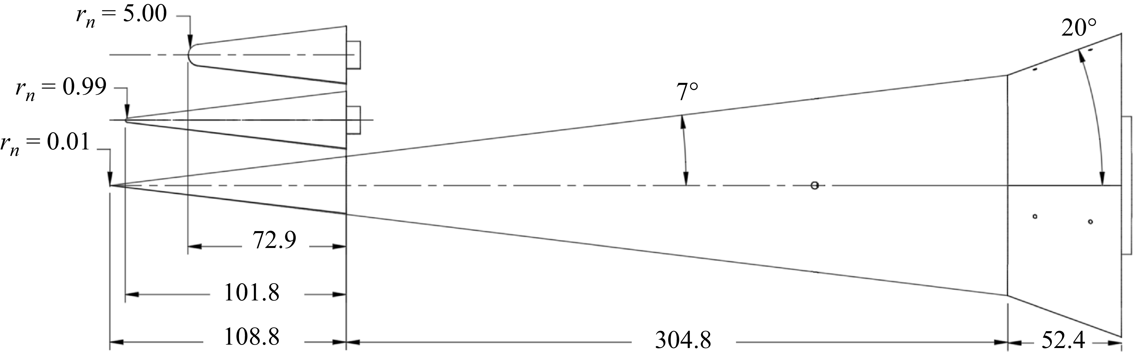
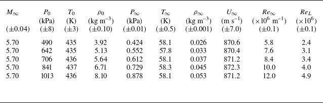


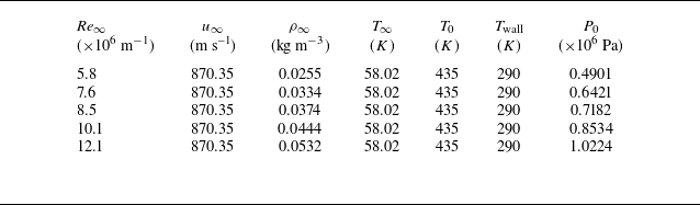


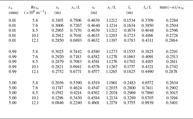


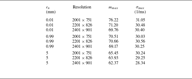


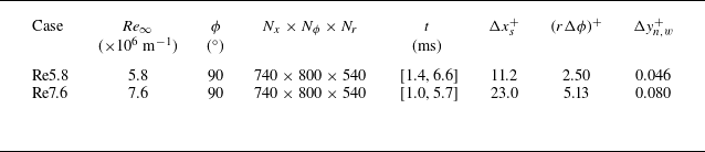
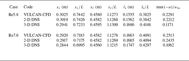

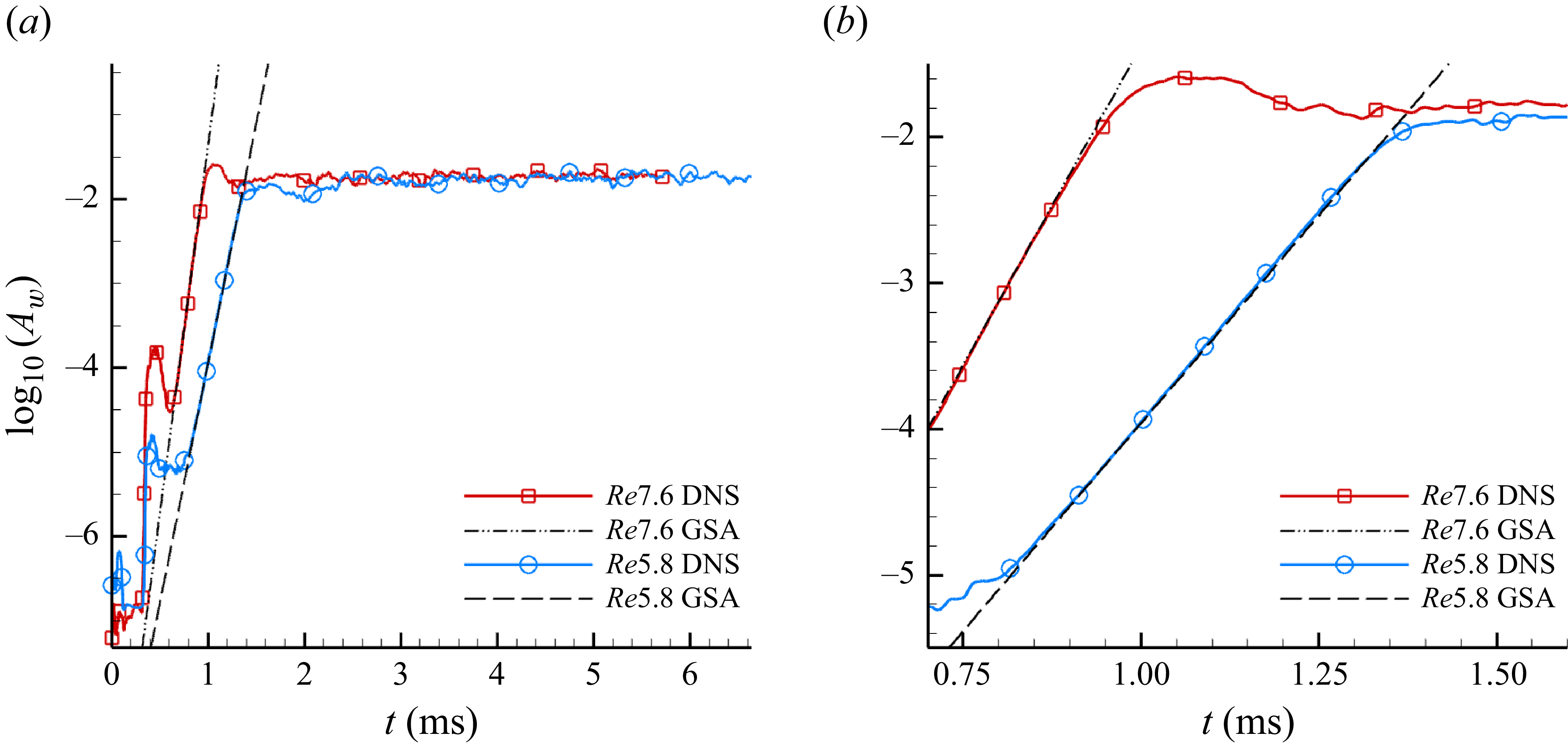


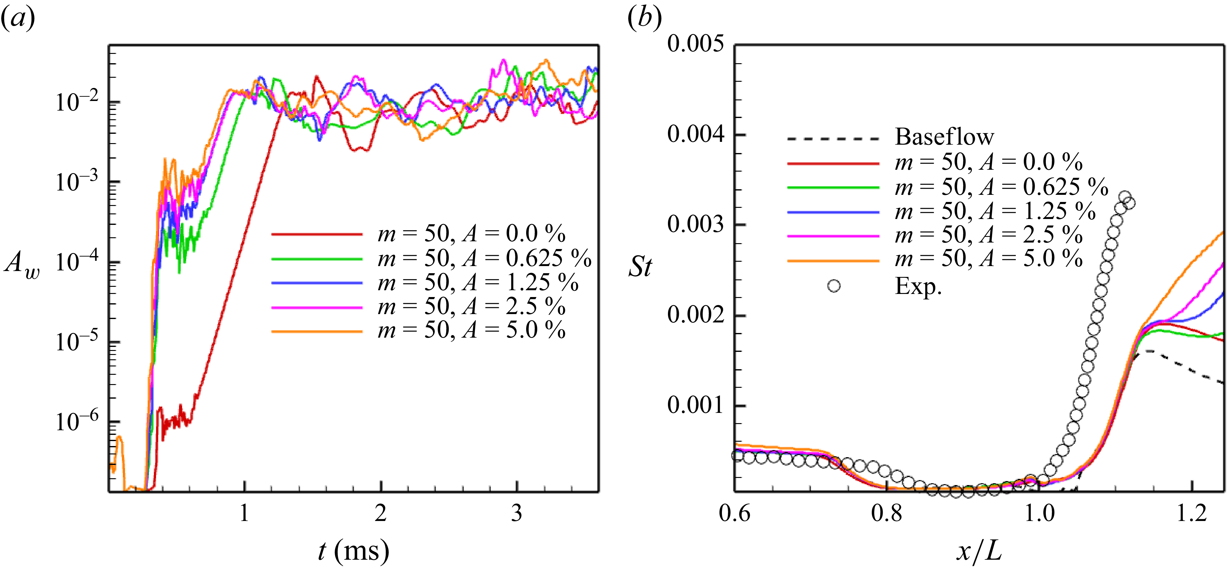


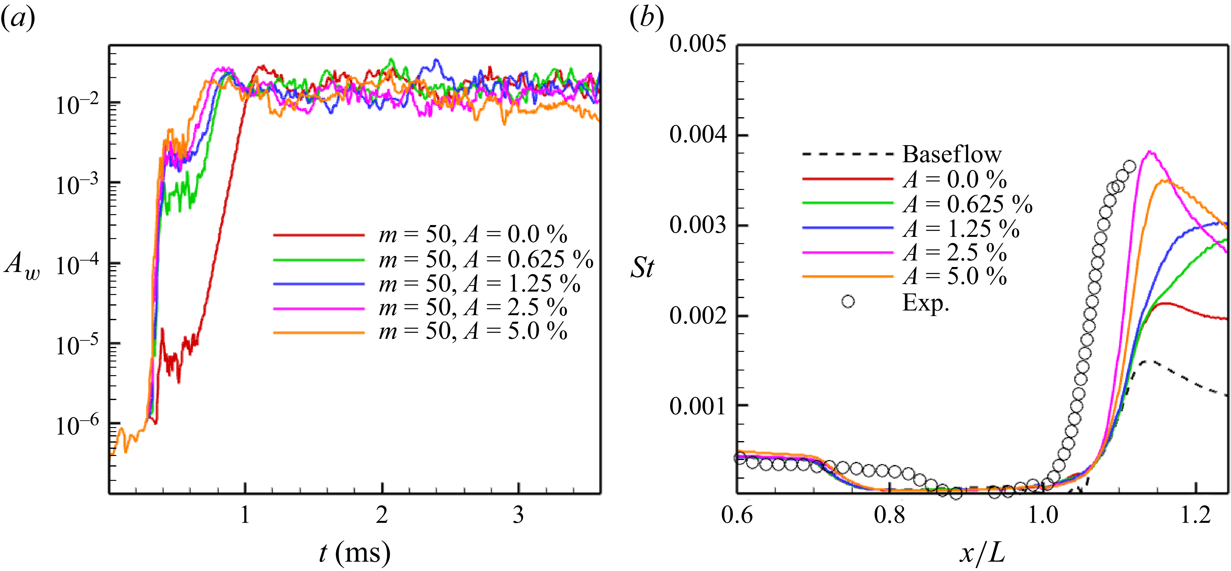


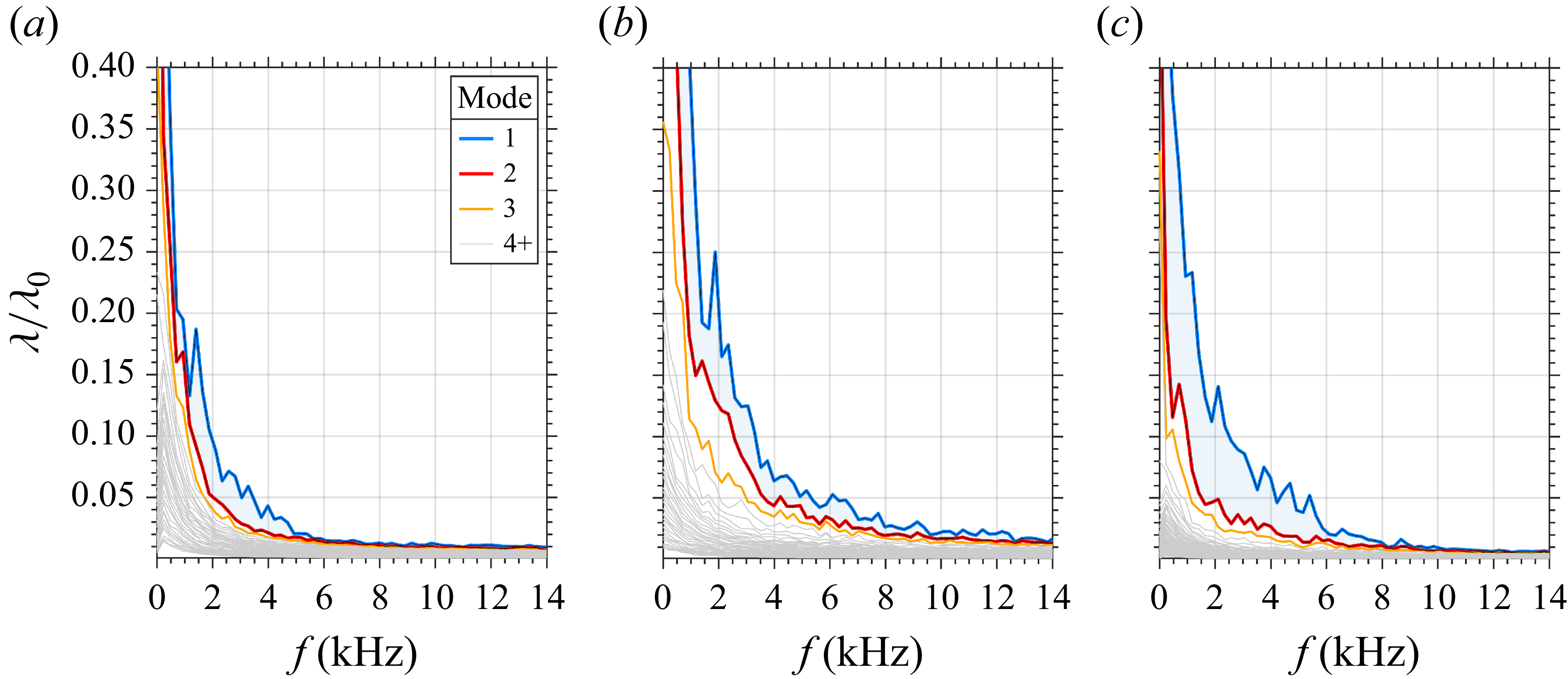


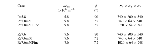
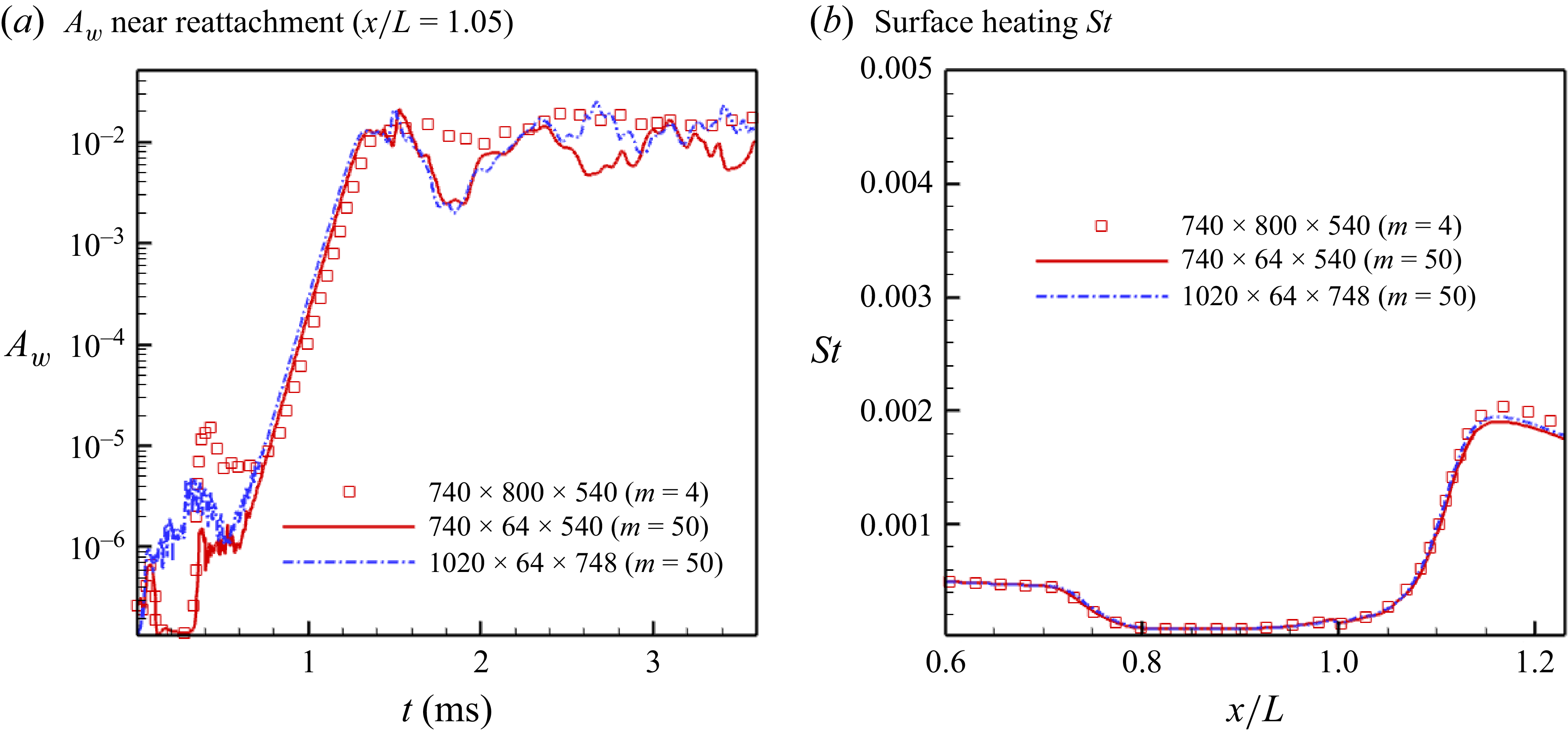


 Open access

