


I. Introduction
Over the last few decades, the corporate sector has become a net provider of capital in many advanced economies (André, Guichard, Kennedy, and Turner (Reference André, Guichard, Kennedy and Turner2007), Chen, Karabarbounis, and Neiman (Reference Chen, Karabarbounis and Neiman2017), and Falato, Kadyrzhanova, Sim, and Steri (Reference Falato, Kadyrzhanova, Sim and Steri2022)). In the United States, this shift has been accompanied by a rapid surge in corporate payouts and savings. Aggregate equity payouts have increased sharply over the last two decades (see Figure 1). The aggregate annual equity payout (dividends plus net share repurchases) rose from $141 billion (in 2010 dollars) between 1987 and 2003 to $525 billion between 2004 and 2019. This rise in payout far outpaced the growth of the economy, as well as the growth of total assets or total income of public companies.
Graphs A–D of Figure 1 plot various measures of equity payouts from 1987 to 2019. Graph A plots the amount of total dividends (DV) by nonfinancial public companies in Compustat. Graph B plots net share repurchases, measured as the purchase of common and preferred stocks (PRSTKC) minus the issuance of stocks (SSTK). Graph C plots the ratio of total net payout (dividends $ + $
net share repurchase) to total assets (AT) and total operating income (OIBDP). In Graph D, the Federal Reserve net payout is based on Table F.103 (nonfinancial corporate business sector) of the FAUS and is measured as dividends (FA106121075) minus net equity issuance (FA103164105). All dollar amounts are in 2010 billion dollars.
$ + $
net share repurchase) to total assets (AT) and total operating income (OIBDP). In Graph D, the Federal Reserve net payout is based on Table F.103 (nonfinancial corporate business sector) of the FAUS and is measured as dividends (FA106121075) minus net equity issuance (FA103164105). All dollar amounts are in 2010 billion dollars.

This rise in corporate payouts has garnered significant attention not only from finance and macroeconomic researchers but also from the popular media and policymakers. Many have raised concerns that corporate equity payouts, especially share repurchases, may enrich shareholders and managers at the expense of workers and the long-term growth of firms and the economy, with some policymakers proposing restrictions or even outright bans on share repurchases.Footnote 1 Proponents of such restrictions frequently contend that tax incentives provided to corporations are spent on payouts rather than new investments or increasing worker salaries. Opponents of such restrictions argue that they would disrupt the natural flow of capital in the economy. For instance, Kevin Hassett, then Chairman of the Council of Economic Advisers, described buybacks as “a natural way our economy recycles cash from old successful firms to new entrepreneurial firms.”Footnote 2 Despite this ongoing debate, there has been scant research into how payout funds circulate within the financial system. Such an investigation would not only aid in understanding the potential consequences of restrictions on corporate payout but would also shed light on the interconnections among financial sectors and the flow of capital in the financial markets (Brainard and Tobin (Reference Brainard and Tobin1968), Gabaix and Koijen (Reference Gabaix and Koijen2025)).
In this article, I take a first step at investigating the flow of payout in the financial system, with a specific focus on the aggregate equity payout of corporations. While the funds distributed by individual companies can be reinvested by the recipient shareholders in the shares of other companies, the net equity payout of the corporate sector as a whole has to go elsewhere. Employing various data sources and empirical strategies, this article provides evidence that a substantial amount of the payout funds flow to the banking sector in the form of deposits and then to bank borrowers.
Using quarterly aggregate data from 1987 to 2019, I document a strong positive relationship between changes in household deposits and net equity payouts by the nonfinancial corporate sector. This positive relationship persists when controlling for various macroeconomic factors such as changes in GDP growth, stock market value, federal funds rates, credit spread, and term spread. The estimation using quarterly aggregate data suggests that a $1 increase in total net equity payout is associated with a contemporaneous $0.4–0.5 increase in household deposits. The effect appears persistent, with deposits remaining heightened for up to 2 years following a payout increase. The results are robust to the use of large, idiosyncratic firm-level payout changes as an instrument for aggregate payout.
Additional analysis shows that net equity payout has a similar association with aggregate deposits that include corporate deposits, suggesting that corporate deposits are not a major funding source for corporate equity payouts. It is also important to recognize that corporations have various margins of adjustment to fund payouts, and investors can deploy the funds through various alternative channels, all of which can influence the economy and the quantity of deposits in complex ways. For example, undistributed corporate funds may be used to purchase Treasury securities from other sectors, such as foreign investors or those newly issued by the federal government, or to undertake new capital investments domestically or internationally. These counterfactual actions could influence many equilibrium outcomes, such as output, savings, the current-account deficit (e.g., Aggarwal, Auclert, Rognlie, and Straub (Reference Aggarwal, Auclert, Rognlie and Straub2023)), and the amount of deposits in the economy. Although detailing these equilibrium adjustments is beyond the scope of this article, the analysis of aggregate data—despite inherent identification challenges—captures their cumulative impact on deposit quantities.
I next turn to regional data to provide further evidence of a causal link between household equity income and deposits. Using dividend income data from the IRS and deposit data from FDIC at the county level, I compare deposit growth across counties that receive varying amounts of dividends. The estimation includes time fixed effects to control for common aggregate shocks and county fixed effects to identify the effect using time-series variation in dividend income and deposit flow within counties. Controlling for county-level observables, including non-dividend income, a $1 increase in taxable dividend income is associated with about a $0.3 increase in county deposits under equal weighting of counties. The point estimate increases substantially when counties are weighted by population, reflecting a more pronounced effect in larger counties.
To isolate variation in county-level dividend income that is independent of local economic shocks, I adopt a shift-share type IV estimation strategy, where the IV is the projected dividend income based on the interaction between a county’s lagged dividend income share and contemporaneous aggregate dividend income. The IV estimation yields precisely estimated coefficients that are slightly larger than the OLS counterparts. Moreover, supplementary analyses show the robustness of the results to various alternative model specifications and estimations. These include comparing deposit growth and dividend income across zip codes within the same county and examining deposit growth across branches owned by the same bank but located in different counties.
In the final part of this article, I investigate the impact of the dividend-driven deposit flow on bank lending. At the bank level, an increase in the amount of dividends received by local residents is associated with a significant rise in bank loans. Further analysis using mortgage and small business lending at the bank-county-level points to an expansion in credit supply as dividend income increases. These findings suggest that funds distributed by large, profitable corporations with free cash flows are, in part, channeled through the banking system to support the activities of bank-dependent firms and households.
The main contribution of this article is to provide evidence on the flow of payout through the banking sector. While in a frictionless world, changes in corporate financial policy do not have real consequences (Stiglitz (Reference Stiglitz1974)), in the real world, capital markets are segmented due to various frictions (e.g., Bolton and Freixas (Reference Bolton and Freixas2000), (Reference Bolton and Freixas2006)). As a result, fluctuations in corporate payouts can alter the supply of capital to different segments of the economy. In the presence of capital market segmentation, even if investors can “pierce through the corporate veil” (Poterba, Hall, and Hubbard (Reference Poterba, Hall and Hubbard1987)), whether savings are held by corporations or households matters. Policies aimed at restricting payouts may distort capital allocation by exacerbating frictions faced by financially constrained firms (e.g., Cooley and Quadrini (Reference Cooley and Quadrini2001), Midrigan and Xu (Reference Midrigan and Xu2014)). Furthermore, this article’s results highlight a flow of funds channel through which certain policies can impact firms that are not directly targeted. For instance, tax holidays for repatriating foreign earnings have been shown to bolster repatriating firms’ payouts rather than their capital expenditure or hiring (e.g., Dharmapala, Foley, and Forbes (Reference Dharmapala, Foley and Forbes2011)). While this outcome runs counter to the intentions of such legislation, the distribution of funds by multinational companies could provide additional funding to the broader economy. Therefore, focusing solely on the behavior of directly targeted firms might not fully capture the broader economic impact of such policies.
This article is related to several strands of literature. First, this article is related to the literature studying the drivers and implications of capital flows in the financial system. In their seminal study, Brainard and Tobin (Reference Brainard and Tobin1968) emphasized the importance of recognizing the interdependence and flow identities in the financial markets. Recently, Gabaix and Koijen (Reference Gabaix and Koijen2025) studied the price impact of flow shocks in the stock market and highlighted the importance of understanding demand shocks and flows, citing corporate payouts as one important example of flow shocks. This article’s results indicate that flow shocks propagate across sectors and asset classes through market clearing and portfolio rebalancing and could impact the real economy beyond the channels that Gabaix and Koijen (Reference Gabaix and Koijen2025) focused on.Footnote 3 In addition, the focus on the flow of capital between the stock market and the banking sector is also related to studies examining the differences and connections between the two sectors (e.g., Allen and Gale (Reference Allen and Gale1997), Boot and Thakor (Reference Boot and Thakor1997), Parlour, Stanton, and Walden (Reference Parlour, Stanton and Walden2012), and Lin (Reference Lin2020)).
Second, this article relates to studies documenting the rise in corporate savings and payouts (e.g., André et al. (Reference André, Guichard, Kennedy and Turner2007), Chen et al. (Reference Chen, Karabarbounis and Neiman2017), Behringer (Reference Behringer2019), Kahle and Stulz (Reference Kahle and Stulz2021), and Falato et al. (Reference Falato, Kadyrzhanova, Sim and Steri2022)). The rise in payout coincides with an increase in corporate income and a decline in investment and capital expenditure (Gutiérrez and Philippon (Reference Gutiérrez and Philippon2017), Kahle and Stulz (Reference Kahle and Stulz2021)).Footnote 4 Several studies document an increase in payout following the Jobs and Growth Tax Relief Reconciliation Act of 2003 that cut the dividend tax rate (e.g., Chetty and Saez (Reference Chetty and Saez2005), Yagan (Reference Yagan2015)) and the American Jobs Creation Act of 2004 that provided a one-time repatriation tax holiday to U.S. multinational companies (e.g., Blouin and Krull (Reference Blouin and Krull2009), Dharmapala et al. (Reference Dharmapala, Foley and Forbes2011)).
Lastly, this article adds to the literature that studies the consumption effects of stock capital gain and dividend income, as well as the reinvestment of dividends (e.g., Poterba (Reference Poterba2000), Baker, Nagel, and Wurgler (Reference Baker, Nagel and Wurgler2007), Hartzmark and Solomon (Reference Hartzmark and Solomon2019), Di Maggio, Kermani, and Majlesi (Reference Di Maggio, Kermani and Majlesi2020), Chodorow-Reich, Nenov, and Simsek (Reference Chodorow-Reich, Nenov and Simsek2021), Meyer and Pagel (Reference Meyer and Pagel2022), and Bräuer, Hackethal, and Hanspal (Reference Bräuer, Hackethal and Hanspal2022)). While the analysis of individual fund utilization is important for understanding personal financial behaviors, it does not inform us of aggregate fund flows. When dividends or proceeds from share sales are reinvested in the stock market, there is necessarily a counterparty who withdraws an equivalent amount from the market. Ultimately, shareholders as a whole cannot reinvest funds into stocks, in the absence of net share issuances by the corporate sector.Footnote 5
II. Data, Measurement, and Summary Statistics
This section begins by describing the data sources, measures, and summary statistics of aggregate corporate equity payout and deposit flow. It then discusses the dividend, deposit, and other data at the county and bank levels. Lastly, it provides an overview of the ownership of U.S. corporate equities and household ownership of financial assets. Definitions of the main variables used in the analysis, along with their sources, are provided in the Supplementary Material.
A. Measures of Aggregate Net Payout and Deposit Flow
The sample period for the aggregate time-series analysis is from 1987 to 2019. The starting year, 1987, was chosen because the prior year marked the end of the phase out of interest rate ceilings on deposits, known as Regulation Q. Deposit growth fluctuated widely in earlier years, partly due to the appeal of Regulation Q that started in the late 1970s and the rapidly evolving inflation environment (Drechsler, Savov, and Schnabl (Reference Drechsler, Savov and Schnabl2021)). The main sample period concludes in 2019 to avoid the confounding effects of the COVID-19 pandemic and the subsequent macroeconomic disruptions and policy responses that caused sharp swings in deposits. Results using the extended sample through 2024 are presented and discussed in Section II.A.3.
I measure quarterly aggregate net corporate equity payout using two data sources: the Federal Reserve’s Financial Accounts of the United States (FAUS) and Compustat. Using the FAUS data, net payout is measured as net dividends plus net share repurchases, computed using Table F.103 (nonfinancial corporate business sector) by subtracting net equity issuance from net dividends (Bianchi, Lettau, and Ludvigson (Reference Bianchi, Lettau and Ludvigson2022), Greenwald et al. (Reference Greenwald, Lettau and Ludvigson2025)). The quarterly flow data at annual rates from FAUS are converted to quarterly rates. Using Compustat data, net payout is measured as the purchase of common and preferred stocks minus the issuance of stocks plus dividends (Eisfeldt and Muir (Reference Eisfeldt and Muir2016)). I then aggregate the net payouts of all nonfinancial firms incorporated in the United States.Footnote 6 Because my focus is on the cash flow between the corporate sector and the household sector, when measuring net share repurchases, I do not include indirect issuance such as the issuance of stocks for employee compensation (e.g., Fried and Wang (Reference Fried and Wang2018b), Fama and French (Reference Fama and French2005), and Boudoukh, Michaely, Richardson, and Roberts (Reference Boudoukh, Michaely, Richardson and Roberts2007)).Footnote 7 The values of aggregate net repurchase and dividends in FAUS are generally higher and more volatile than those from Compustat. In addition to the fact that FAUS data include payouts made by both public and private companies, there are various other important differences between the two measures.Footnote 8 In the estimation using quarterly aggregate data, I use the net payout from FAUS as the main measure but also report results using Compustat payout as a robustness check.
I measure quarterly aggregate deposit flow using data from both FAUS and FDIC’s Quarterly Banking Profile (QBP). Using the FAUS data, deposit flow is the sum of flows of checkable deposits, currency, and time and savings deposits held by households and nonprofit organizations. Using the QBP data, deposit flow is simply the difference in total domestic deposits between two consecutive quarters.
A portion of this article’s analysis uses aggregate dividend and deposit data at the monthly frequency. Monthly deposit data are from the Federal Reserve’s Table H.8, whereas dividend income and total personal income data are from the Bureau of Economic Analysis (BEA) NIPA Table 2.6. In addition, monthly dividend payment data from CRSP are used. Following the literature (e.g., Boudoukh et al. (Reference Boudoukh, Michaely, Richardson and Roberts2007), Kahle and Stulz (Reference Kahle and Stulz2021)), I include stocks traded on NYSE, AMEX, or NASDAQ with CRSP share codes of 10 or 11 and a first 2-digit distribution code of 12.
Panel A of Table 1 reports the summary statistics of the aggregate variables at the quarterly frequency. On average, deposits increase by $70 billion per quarter, and quarterly net equity payout is $142 billion. All dollar amounts in this article are expressed in 2010 dollars. Deposit flow, net equity payout, and the change in stock market value are 0.5%, 1.0%, and 1.7% of lagged GDP on average, respectively. Panel B reports the summary statistics of variables at the monthly frequency.

Figure 1 plots the time series of various measures of aggregate payouts since 1987. Graph A shows that dividends paid by nonfinancial firms in the Compustat/CRSP universe have increased dramatically since the early 2000s, as documented by Kahle and Stulz (Reference Kahle and Stulz2021). It also shows that the sharp increase in dividend payment is not simply due to the growth of the overall economy, as dividends paid by public companies as a share of GDP have also risen substantially since the early 2000s. Graph B shows a similar trend in net share repurchases, which also exhibit greater variability than dividends. Graph C shows that net payout (dividends $ + $
net share repurchases) as a share of total assets or total income also rose substantially after 2004, suggesting that corporations have been paying out more of the income that they generate (Kahle and Stulz (Reference Kahle and Stulz2021)). Finally, as noted above, Graph D shows that the total net equity payout as measured using the FAUS data is substantially higher than that using Compustat data. Nonetheless, the two series generally track each other, and FAUS data also show a substantial increase in net payout after 2004.
$ + $
net share repurchases) as a share of total assets or total income also rose substantially after 2004, suggesting that corporations have been paying out more of the income that they generate (Kahle and Stulz (Reference Kahle and Stulz2021)). Finally, as noted above, Graph D shows that the total net equity payout as measured using the FAUS data is substantially higher than that using Compustat data. Nonetheless, the two series generally track each other, and FAUS data also show a substantial increase in net payout after 2004.
B. Dividend Income, Deposits, Loans, and Other County- and Bank-Level Data
Deposit data at the county level are from the FDIC’s Summary of Deposits, which reports the total branch deposits for FDIC-insured institutions as of June 30 every year since 1994. The income and population data are from the BEA. The difference between the BEA income and the IRS dividend income is used to measure non-dividend income.
The dividend income data at the county and zip-code level are from the IRS’s Statistics of Income (SOI). The county-level data are available since 1989, whereas the zip-code level dividend income data are available since 2004. The IRS data cover all households that file tax returns, which allows for measuring dividend income at a very granular level. While most dividends received by households are distributed by publicly traded companies, a small fraction could also come from privately owned C corporations.Footnote 9 The dividend income data do not capture dividends received through nontaxable accounts such as retirement plans, which are typically reinvested and therefore not expected to influence local deposit flows significantly.
Panel C of Table 1 reports the summary statistics of the county-level variables. The average real annual deposit growth rate is 1.2%. Dividend scaled by lagged deposits has an average of 2.1%. Non-dividend income is about 2.4 times the value of lagged county deposits. Dividend as a share of total adjusted gross income is 1.7% on average.
I obtain bank balance sheet data from the Consolidated Report of Condition and Income filed by banks, commonly known as “call reports.” The sample is restricted to commercial banks (rssd9048 = 200). I obtain deposits (rcon2200), loans (rcon1400, or rcon2122 $ + $
rcon2123 if rcon1400 is missing), C&I loans (rcon1766, or rcon1763
$ + $
rcon2123 if rcon1400 is missing), C&I loans (rcon1766, or rcon1763 $ + $
rcon1764 if rcon1766 is missing), real estate loans (rcon1410, or the sum of rconf158, rconf159, rcon1420, rcon1797, rcon5367, rcon5368, rcon1460, rconf160, and rconf161 if rcon1410 is missing), securities (sum of rcon1754 and rcon1773), total assets (rcon2170), equity (rcon3210), and income (riad4340). The rcfd series values are used if the rcon values are missing. I exclude banks with negative or missing deposits, loans, or equity, or if these values are greater than total assets. I exclude bank-year observations in which a bank acquired another bank during the year and those with asset growth below the 1st or above the 99th percentile of the distribution over the sample period. The summary statistics of the key variables used in the bank-level analysis are reported in Panel D of Table 1.
$ + $
rcon1764 if rcon1766 is missing), real estate loans (rcon1410, or the sum of rconf158, rconf159, rcon1420, rcon1797, rcon5367, rcon5368, rcon1460, rconf160, and rconf161 if rcon1410 is missing), securities (sum of rcon1754 and rcon1773), total assets (rcon2170), equity (rcon3210), and income (riad4340). The rcfd series values are used if the rcon values are missing. I exclude banks with negative or missing deposits, loans, or equity, or if these values are greater than total assets. I exclude bank-year observations in which a bank acquired another bank during the year and those with asset growth below the 1st or above the 99th percentile of the distribution over the sample period. The summary statistics of the key variables used in the bank-level analysis are reported in Panel D of Table 1.
I obtain mortgage loan data from the Home Mortgage Disclosure Act (HMDA) data sets. For each bank-county-year observation, I calculate the total dollar amount of originated home purchase loans that were not sold in the same year (loan purpose = 1, action type = 1, purchaser type = 0). Banks in the HMDA data are matched to Call Report filers using agency-specific respondent identifiers based on their regulatory authority. To ensure reliable matching between HMDA and Call Report data, I exclude bank-year observations in which the total volume of home-purchase mortgages originated and retained (i.e., not sold in the same year) exceeds the year-end stock of residential mortgage loans reported in the Call Reports.
Small business loan data at the bank-county level are obtained from the Federal Financial Institutions Examination Council (FFIEC). Small business loans are defined by FFIEC as loans whose original amounts are $1 million or less. Under the Community Reinvestment Act, all institutions regulated by the OCC, Federal Reserve, and FDIC that meet the asset size threshold are subject to data collection and reporting requirements.
C. Accounting for Net Equity Payout
This section presents and discusses some facts about the ownership of U.S. corporate equities and household ownership of financial assets. They serve as a useful context and motivation for the main analyses.
By a simple cash flow accounting identity, when corporations as a whole pay out $1 of dividend or repurchase $1 of shares, equity owners as a whole must receive the $1. If all owners have the same propensity to reinvest dividends or sell shares back to companies, the money flows to each sector of owners proportional to its ownership share. However, if some owners are more passive (i.e., more likely to reinvest dividends and less likely to sell shares), the more active sectors receive more than their ownership share. Figure 2 plots the ownership of U.S. corporate equity from 1987 to 2019, using data from FAUS.Footnote 10 It shows that household ownership of total U.S. equity (excluding retirement accounts) has declined from around 50% to just below 40% during this period. About one third is owned by retirement plans, including both defined contribution and defined benefit pension plans, as well as individual retirement accounts. Foreign investors’ share has increased steadily during this period, reaching almost 15% in 2019, whereas nonfinancial corporations and financial corporations such as banks and insurance companies own only a small fraction. Although one might expect some groups of investors, such as pension funds, to be more passive, there is no significant correlation between corporate net equity payout and changes in sector ownership at the quarterly frequency.Footnote 11
Figure 2 plots the ownership of U.S. corporate equities from 1987 to 2019. Source: Financial Accounts of the United States (FAUS). Ownership by the household sector: direct ownership (LM153064105) + indirect ownership through mutual funds (LM653064155) $ - $
equity held in individual retirement accounts (IRAs). IRA: (mutual funds (LM653131573) and other self-directed accounts (LM153131575) in IRA) × 0.7. Pension: defined benefit pension plans: held directly (LM573064143 + LM343064135 + LM223064145) + indirectly through mutual funds ((LM573064243 + LM223064243) × LM653064100/LM654090000) + private defined contribution pension funds; corporate equities held directly and indirectly through mutual funds (LM573064175) + federal government retirement funds; corporate equities held by thrift savings plan (LM343064125) + state and local government employee retirement funds; corporate equities held indirectly through mutual funds (LM223064213) + life insurance companies; corporate equities held directly and indirectly through mutual funds (LM543064153). Rest of the world: LM263064105. Nonfinancial corporations: LM103064103. Financial firms such as banks and insurance companies: LM763064105 + LM543064105 + LM513064105. ETF: LM563064100.
$ - $
equity held in individual retirement accounts (IRAs). IRA: (mutual funds (LM653131573) and other self-directed accounts (LM153131575) in IRA) × 0.7. Pension: defined benefit pension plans: held directly (LM573064143 + LM343064135 + LM223064145) + indirectly through mutual funds ((LM573064243 + LM223064243) × LM653064100/LM654090000) + private defined contribution pension funds; corporate equities held directly and indirectly through mutual funds (LM573064175) + federal government retirement funds; corporate equities held by thrift savings plan (LM343064125) + state and local government employee retirement funds; corporate equities held indirectly through mutual funds (LM223064213) + life insurance companies; corporate equities held directly and indirectly through mutual funds (LM543064153). Rest of the world: LM263064105. Nonfinancial corporations: LM103064103. Financial firms such as banks and insurance companies: LM763064105 + LM543064105 + LM513064105. ETF: LM563064100.

How might shareholders use the payout funds that are not reinvested in stocks? Investors can use these funds to increase consumption, pay down debt, or save in other forms of financial assets. In a frictionless world, whether a dollar is paid out or saved by corporations on behalf of households should not matter for households’ consumption or saving decisions. However, in reality, due to various frictions or behavioral reasons, households may choose to increase consumption upon receiving payout funds (Baker et al. (Reference Baker, Nagel and Wurgler2007)), and they may save the money in different financial assets than those typically held by corporations.
Supplementary Material Figure A2 depicts the composition of non-retirement financial assets held by U.S. households, using FAUS data. This composition varies considerably over time, primarily due to fluctuations in stock returns. On average, stocks (including both directly held and indirectly held through mutual funds) make up 42% of total non-retirement financial assets, while deposits represent 30%, followed by other fixed-income investments such as government and corporate bonds, loans, and money market mutual funds.
FAUS data do not provide information about the joint ownership of these different types of assets at the household level. Examining disaggregated data reveals that there does not appear to be a significant overlap between stock and bond ownership at the household level. For instance, according to the 2016 Survey of Consumer Finance data, of the nearly 20% of households that own stocks in non-retirement accounts (either directly or indirectly through mutual funds), only a third report any ownership of bonds or bond mutual funds. Even among the top quartile of stock owners (with a market value of stocks over a quarter million), only about half report owning any bonds. In contrast, nearly all stock owners report owning deposits.Footnote 12 Thus, deposits emerge naturally as a potentially important destination for payout funds.Footnote 13
While the portfolio rebalancing channel is the most straightforward interpretation of the relationship between equity and deposit flows, other indirect transmission mechanisms also exist. Specifically, because deposits function as a means of payment, they are closely connected to economic activity. For example, when households spend their dividend income, that expenditure becomes someone else’s income, which is then spent or saved in turn (e.g., Auclert, Rognlie, and Straub (Reference Auclert, Rognlie and Straub2023), Aggarwal et al. (Reference Aggarwal, Auclert, Rognlie and Straub2023)). Some of these savings may end up as deposits. However, at the aggregate level, we can abstract from these sequential transactions if we assume a representative household that makes spending and investment decisions. Ultimately, the accumulation of savings in deposits after multiple transaction rounds is intrinsically linked to the portfolio rebalancing channel.
III. Results
A. Aggregate Payout and Deposit Flow
This section examines the relationship between aggregate corporate equity payout and deposit flows. It starts by estimating how deposit growth varies with payout at the quarterly frequency, controlling for various macroeconomic factors. It then presents evidence from an IV estimation strategy instrumenting aggregate payout with large, idiosyncratic firm-level payouts. In addition, the section discusses the results of several supplementary analyses, including corporate deposits, household holding of non-deposit fixed-income assets, deposit prices, and debt payouts.
1. Quarterly Payout and Deposit Flow
Figure 3 shows that the quarterly deposit flow of the household sector is positively correlated with the net equity payout of the nonfinancial corporate business sector during the period of 1987 to 2019. This positive correlation is not obvious a priori, as corporate equity payouts tend to be procyclical (Jermann and Quadrini (Reference Jermann and Quadrini2012), Begenau and Salomao (Reference Begenau and Salomao2018)), while deposit growth does not have a significant correlation with GDP growth and tends to increase during stock market downturns (Lin (Reference Lin2020)). To estimate the relationship between the two variables, I regress changes in household sector deposits on net payout, both scaled by lagged GDP, along with other macroeconomic factors:
 $$ \varDelta Deposit{s}_t/ GD{P}_{t-1}=\alpha +\beta Net\ payou{t}_t/ GD{P}_{t-1}+\gamma {X}_t+{\epsilon}_t. $$
Figure 3 plots the quarterly flow of household deposits (FA153020005 + FA153030005) against net corporate payout (FA106121075 $ - $
FA103164105). All values are in 2010 dollars. Data source: Financial Accounts of the United States (FAUS).
$ - $
FA103164105). All values are in 2010 dollars. Data source: Financial Accounts of the United States (FAUS).

Table 2 reports the estimation results. Column 1 reports that, without any controls, the coefficient of net payout is 0.49, suggesting that a $1 increase in net payout is associated with a $0.49 increase in deposits. The R 2 of 16.4% from this univariate regression also suggests an important role of payout in explaining changes in deposits. I next add various measures of macroeconomic conditions as control variables. These include contemporaneous GDP growth, changes in stock values (scaled by lagged GDP), changes in federal funds rate, changes in credit spread, changes in inflation, changes in unemployment rate, and changes in term spread. Column 2 reports that the coefficient of net payout remains similar with the addition of these controls. Therefore, the positive relationship between corporate equity payout and deposits observed in Figure 3 cannot be attributed to fluctuations in economic, monetary, or financial conditions.Footnote 14
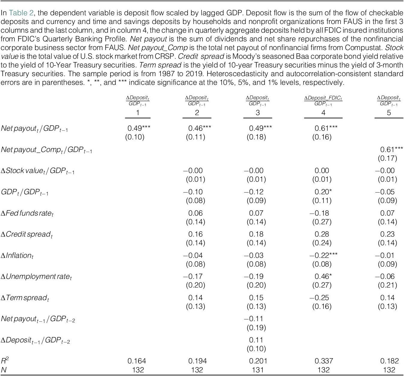
The deposit measure used in the analysis above includes both categories reported in the FAUS data: i) checkable deposits and currency and ii) time and savings deposits. I next examine these two components separately. The last 2 columns of Supplementary Material Table A2 report that the positive relationship between payout and deposit flow is concentrated on time and savings deposits, which are more likely to serve as substitutes for stock investment. In contrast, the coefficient on net payout is close to zero when checkable deposits and currency are examined.Footnote 15
I next examine the dynamics of deposits following changes in payout. In column 3, the lagged payout scaled by GDP and the lagged dependent variable are added to the estimation. Deposit growth does not exhibit a significant first-order autocorrelation at the quarterly frequency. Lagged payout during quarter $ t-1 $
has an insignificant effect on deposit growth in quarter
$ t-1 $
has an insignificant effect on deposit growth in quarter $ t $
, whereas the coefficient of payout in quarter
$ t $
, whereas the coefficient of payout in quarter $ t $
increases slightly. In addition, untabulated results show that when net payout from quarter
$ t $
increases slightly. In addition, untabulated results show that when net payout from quarter $ t-4 $
to quarter
$ t-4 $
to quarter $ t $
are all included, time
$ t $
are all included, time $ t $
payout has a coefficient of 0.46 and a p-value of 0.021, whereas the coefficients of all four lagged payouts are close to zero and statistically insignificant. This indicates that deposit growth is significantly associated only with contemporaneous net corporate payout, with no subsequent reversal in the effect.
$ t $
payout has a coefficient of 0.46 and a p-value of 0.021, whereas the coefficients of all four lagged payouts are close to zero and statistically insignificant. This indicates that deposit growth is significantly associated only with contemporaneous net corporate payout, with no subsequent reversal in the effect.
To provide further evidence on the persistence of the impact of payout on deposits, I estimate the impulse responses of deposits to innovations in payout using the local projections approach of Jordà (Reference Jordà2005). Specifically, at each horizon $ h=0,\dots, 8 $
, the log change in deposits from quarter
$ h=0,\dots, 8 $
, the log change in deposits from quarter $ t-1 $
to
$ t-1 $
to $ t+h $
is regressed on payout scaled by GDP in quarter
$ t+h $
is regressed on payout scaled by GDP in quarter $ t $
as well as its 2 lags. Figure 4 plots the coefficients of quarter
$ t $
as well as its 2 lags. Figure 4 plots the coefficients of quarter $ t $
payout. An increase in payout leads to an immediate increase in deposits, and the effect persists for up to 2 years. A 1-percentage-point increase in the payout-to-GDP ratio is associated with a roughly 2% increase in deposits.
$ t $
payout. An increase in payout leads to an immediate increase in deposits, and the effect persists for up to 2 years. A 1-percentage-point increase in the payout-to-GDP ratio is associated with a roughly 2% increase in deposits.
Figure 4 plots the coefficients $ {\beta}_0^h $
s and the 90% confidence intervals from the regression,
$ {\beta}_0^h $
s and the 90% confidence intervals from the regression, $ Ln{(deposit)}_{t+h}- Ln{(deposit)}_{t-1}=\alpha +\sum \limits_{i=0}^2{\beta}_i^h\Delta {\frac{Payout}{GDP}}_{t-i}+{\unicode{x025B}}_t $
, for
$ Ln{(deposit)}_{t+h}- Ln{(deposit)}_{t-1}=\alpha +\sum \limits_{i=0}^2{\beta}_i^h\Delta {\frac{Payout}{GDP}}_{t-i}+{\unicode{x025B}}_t $
, for $ h=0,\dots, 8 $
, where
$ h=0,\dots, 8 $
, where $ t $
indexes quarters. Newey–West standard errors with
$ t $
indexes quarters. Newey–West standard errors with $ h $
order of autocorrelation are used. The sample period is from 1987 to 2019.
$ h $
order of autocorrelation are used. The sample period is from 1987 to 2019.

The results so far show a strong positive association between net corporate equity payout and household holdings of deposits. One might wonder whether the rise in corporate payout is associated with a decline in corporate deposits, to the extent that firms use their deposit holding to fund some of the payout.Footnote 16 To address this possibility, in column 4, I replace FAUS household deposits with FDIC total domestic deposits, which include both household and corporate deposits at all FDIC-insured institutions (and are on average about 14% larger than FAUS household deposits). The coefficient of net payout is 0.61 and highly statistically significant. This finding suggests that any decline in corporate deposits is small relative to the increase in household deposits as corporate equity payout rises.Footnote 17
Lastly, the aggregate payout of nonfinancial firms in Compustat is used as an alternative to FAUS payout. Column 5 reports that the coefficient of Compustat payout scaled by GDP is 0.61 and significant at the 1% level.
2. IV Estimation Based on Large Idiosyncratic Payouts
The results in the previous section show a robust positive association between net corporate equity payout and the quantity of deposits in the economy. Of course, firms do not adjust payouts randomly and one naturally worries that the factors that lead firms to adjust payouts (cash flows, investment opportunities, taxation, etc.) could be correlated with deposits through some alternative channels. While it is difficult to establish causality using aggregate data, this section seeks to partially address concerns about omitted variables by exploiting large, idiosyncratic firm-level payouts as an instrumental variable for aggregate payouts, in the spirit of the granular instrumental variable approach of Gabaix and Koijen (Reference Gabaix and Koijen2024).
As a prominent example, in December 2004, Microsoft distributed a dividend of $33.5 billion, of which $32 billion was a one-time special dividend. This accounted for more than 50% of all dividends paid out by CRSP firms that month. Thus, Microsoft’s special dividend payout represents a significant shock to the aggregate dividend in December 2004, and it can be considered plausibly exogenous to aggregate deposit growth during that month. Importantly, not all firms increased dividends significantly that month. In fact, the median firm maintained the same amount of dividend between September and December, and the 75th percentile dividend growth rate is merely 1%.
To begin, I define a simple measure of abnormal changes in dividend payments at the firm level:
 $$ \Delta {Div}_{i,t}={Div}_{i,t}-{Div}_{i,t-3}\times Median{\left(\frac{\Delta {Div}_{j,t}}{Div_{j,t-3}}\right)}_t, $$
where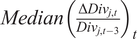 $ Median{\left(\frac{\Delta {Div}_{j,t}}{Div_{j,t-3}}\right)}_t $
is the median dividend growth rate from month
$ Median{\left(\frac{\Delta {Div}_{j,t}}{Div_{j,t-3}}\right)}_t $
is the median dividend growth rate from month $ t-3 $
to month
$ t-3 $
to month $ t $
of all dividend-paying firms, and is used as the benchmark for the “normal” dividend growth rate. (As noted below, the results are robust to using dividend growth at the 75th or 90th percentile as the benchmark.) I then aggregate the abnormal dividend payments of the top payers every month and use it as an instrument for the actual dividend payout in that month. In what follows, I report the results based on the top 3% abnormal dividend payments in a given month but note below that the results are robust to alternative cutoffs.Footnote
18 The total abnormal dividend payment in a given month is large when some major dividend payers raise their dividends substantially relative to other dividend-paying firms in the same month. If these large increases in dividends are idiosyncratic and uncorrelated with other determinants of aggregate deposits, as appears to be the case for Microsoft’s special dividend in December 2004, the exclusion condition will be satisfied.
$ t $
of all dividend-paying firms, and is used as the benchmark for the “normal” dividend growth rate. (As noted below, the results are robust to using dividend growth at the 75th or 90th percentile as the benchmark.) I then aggregate the abnormal dividend payments of the top payers every month and use it as an instrument for the actual dividend payout in that month. In what follows, I report the results based on the top 3% abnormal dividend payments in a given month but note below that the results are robust to alternative cutoffs.Footnote
18 The total abnormal dividend payment in a given month is large when some major dividend payers raise their dividends substantially relative to other dividend-paying firms in the same month. If these large increases in dividends are idiosyncratic and uncorrelated with other determinants of aggregate deposits, as appears to be the case for Microsoft’s special dividend in December 2004, the exclusion condition will be satisfied.
Figure 5 plots seasonally adjusted aggregate monthly dividend payments by publicly traded firms in CRSP, along with total abnormal dividend payments in the top 3% for a given month, both scaled by lagged GDP. It shows that sharp increases in aggregate dividend payments, such as those in December 2004 and 2012, are frequently the result of large idiosyncratic increases in dividends by individual firms. The sharp increase in December 2004 was almost entirely driven by Microsoft’s special dividend payment discussed above, whereas the increase in December 2012 was driven by some firms’ decision to raise dividends ahead of a potential dividend income tax rate hike in 2013. However, there are also times when a sharp rise in total dividends is not accompanied by large idiosyncratic dividend payments. The precise timing of dividend payments at the monthly frequency also helps rule out alternative explanations. For example, while changes in dividend income tax rate could affect the amount of bank deposits through other channels, there is no obvious reason to expect such impacts to coincide exactly with the months when large special dividends are paid.
Figure 5 plots the aggregate monthly dividend payment by firms traded on NYSE, AMEX, or NASDAQ with CRSP shares codes 10 or 11 and first 2-digit distribution code (distcd) 12, and the total top 3% abnormal increases in monthly dividend payments, both scaled by lagged GDP. Abnormal change in monthly dividend payment is defined as $ \Delta {Div}_{i,t}={Div}_{i,t}-{Div}_{i,t-3}\times Median{\left(\frac{\Delta {Div}_{j,t}}{Div_{j,t-3}}\right)}_t $
, where
$ \Delta {Div}_{i,t}={Div}_{i,t}-{Div}_{i,t-3}\times Median{\left(\frac{\Delta {Div}_{j,t}}{Div_{j,t-3}}\right)}_t $
, where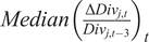 $ Median{\left(\frac{\Delta {Div}_{j,t}}{Div_{j,t-3}}\right)}_t $
is the median dividend growth rate from month
$ Median{\left(\frac{\Delta {Div}_{j,t}}{Div_{j,t-3}}\right)}_t $
is the median dividend growth rate from month $ t-3 $
to month
$ t-3 $
to month $ t $
of all dividend-paying firms.
$ t $
of all dividend-paying firms.

The model estimated is
 $$ {\displaystyle \begin{array}{c}\Delta {Deposits}_t/{GDP}_{t-1}=\alpha +{\beta}_1{Dividend}_t/{GDP}_{t-1}\\ {}\hskip1.5em +{\beta}_2 Other\;{Income}_t/{GDP}_{t-1}+\gamma {X}_t+{\unicode{x025B}}_t,\end{array}} $$
where $ \Delta {Deposits}_t $
is the change in monthly deposits held by all commercial banks from the Federal Reserve’s H8 releases and the main independent variable of interest
$ \Delta {Deposits}_t $
is the change in monthly deposits held by all commercial banks from the Federal Reserve’s H8 releases and the main independent variable of interest $ {Dividend}_t $
is the aggregate monthly dividend income from BEA NIPA.
$ {Dividend}_t $
is the aggregate monthly dividend income from BEA NIPA. $ Other\;{Income}_t $
is the personal income minus dividend income from the BEA. As the GDP data are not available at the monthly frequency, GDP in the previous quarter is used as the scaling variable (the results are robust to using alternative scaling variables such as lagged total monthly personal income from the BEA.)
$ Other\;{Income}_t $
is the personal income minus dividend income from the BEA. As the GDP data are not available at the monthly frequency, GDP in the previous quarter is used as the scaling variable (the results are robust to using alternative scaling variables such as lagged total monthly personal income from the BEA.) $ X $
includes other control variables, including monthly stock returns, changes in federal funds rate, credit spread, inflation, unemployment rate, and term spread, as well as month-of-the-year dummies.
$ X $
includes other control variables, including monthly stock returns, changes in federal funds rate, credit spread, inflation, unemployment rate, and term spread, as well as month-of-the-year dummies.
Before proceeding to the IV estimation, I first report the results of the OLS estimation of equation (3). The first column of Panel A of Table 3 reports that the coefficient of dividend income is 0.74 and highly statistically significant. The magnitude of the effect is larger than the estimates from Table 2, which use aggregate quarterly payout data.
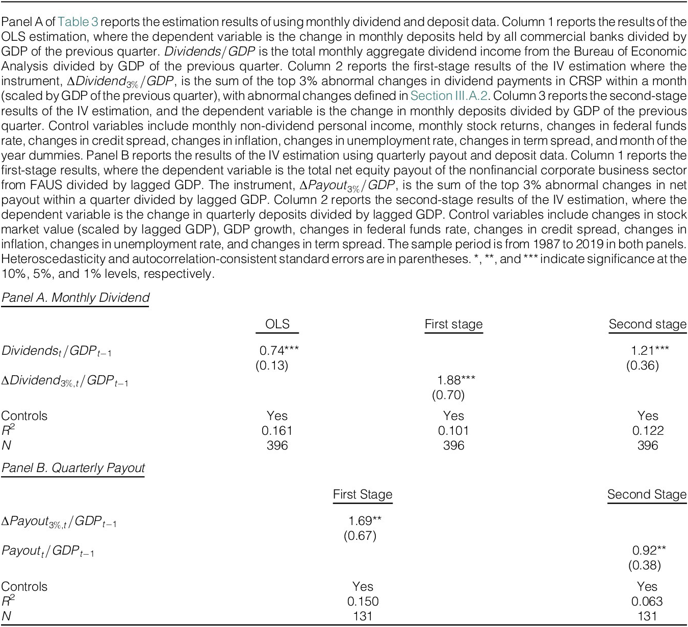
The second column reports the first stage result of the IV estimation. It shows a significantly positive relationship between the abnormal monthly dividend payments of the top 3% and aggregate monthly dividends. The third column presents the second stage results. The instrumented dividend payout has a significantly positive effect on deposit growth. A one-dollar incremental dividend is associated with a contemporaneous $1.21 change in aggregate deposits.Footnote
19 To examine the dynamics of this effect, I replace the change in deposits from month $ t-1 $
to
$ t-1 $
to $ t $
on the left-hand side of equation (3) with the change in deposits from month
$ t $
on the left-hand side of equation (3) with the change in deposits from month $ t-1 $
to up to 5 months after
$ t-1 $
to up to 5 months after $ t $
and rerun the IV estimation using the same right-hand side variables and the same instrument. The impulse responses plotted in Supplementary Material Figure A3 show no evidence of a reversal in the effect in subsequent months.
$ t $
and rerun the IV estimation using the same right-hand side variables and the same instrument. The impulse responses plotted in Supplementary Material Figure A3 show no evidence of a reversal in the effect in subsequent months.
I next apply the same IV strategy to estimate the relationship between quarterly net payout and deposit flow, which is explored using OLS estimation in Section III.A.1. The IV is the aggregate abnormal payouts that are in the top 3% among all nonfinancial publicly traded firms in the Compustat/CRSP universe, scaled by lagged GDP. The only modification to equation (2) is the use of the 75th percentile of payout growth as the benchmark for normal payout growth, instead of the median, due to mostly negative median values. Panel B reports the first- and second-stage results, where the instrumented variable is the net payout from FAUS divided by lagged GDP. Column 2 reports that the estimated coefficient on payout is 0.92 and significant at the 5% level.Footnote 20
Overall, the analysis using aggregate payout and deposit data reveals that a large fraction of the payout funds flows into the banking sector in the form of deposits. An advantage of using macro-level data is that they capture the net aggregate effects of individual behaviors and various adjustments in general equilibrium. Di Maggio et al. (Reference Di Maggio, Kermani and Majlesi2020) reported a small response of bank accounts (deposits) to changes in dividend income and a large fraction of dividends reinvested in the stock market, based on household level data.Footnote 21 While household-level data are useful to understand the behavior of individuals, they do not necessarily map directly into aggregate outcomes. For example, when someone reinvests dividends in the stock market—whether by purchasing shares of the same firm or of a different firm—there must be a counterparty who sells shares and receives cash, which may ultimately be deposited in the banking system. As a result, estimates based on individual responses to dividend income shocks can understate the aggregate flow into bank deposits and overstate the extent to which dividends are reinvested in equities. In fact, shareholders as a whole cannot reinvest dividends into stocks, absent net share issuances by the corporate sector.
3. Additional Results
The previous sections present evidence on how deposit quantities change with corporate equity payouts. A natural follow-up question is whether deposit rates also adjust to payout-driven fluctuations in deposit demand. To investigate this, I calculate the average interest rates banks pay on their deposits using the call report data (Acharya and Mora (Reference Acharya and Mora2015), Drechsler et al. (Reference Drechsler, Savov and Schnabl2017)) and examine the relationship between aggregate payout and the deposit spread—measured as either the difference between the federal funds rate and the average deposit rate or the difference between the 1-year Treasury yield and the deposit rate.
Supplementary Material Table A5 reports the results. Columns 1 and 2 report results from level specifications, where deposit spread is regressed on net payout (scaled by GDP) and the level of control variables. The coefficient of net payout is positive and statistically significant at the 1% level when the federal funds rate is used as the benchmark, suggesting that deposit spreads tend to be elevated during periods of high payouts. However, when the 1-year Treasury yield is used as the benchmark instead, the coefficient becomes substantially smaller and statistically insignificant.
Columns 3 and 4 report results from first-difference specifications, where changes in deposit spread are regressed on changes in net payout and controls. In both cases, the coefficient on net payout is close to zero and statistically insignificant. These findings suggest that deposit rates do not adjust quickly in response to payout-driven fluctuations in deposit demand. Overall, the response of deposit rates to corporate payouts appears muted, a pattern consistent with the well-documented stickiness of deposit rates, particularly in response to short-term fluctuations in deposit flows.
This article mainly focuses on the flow of payout funds into the banking sector in the form of deposits. However, the money could also flow into other types of financial assets, such as non-deposit fixed-income securities. To explore this possibility, I examine the correlation between net equity payout and changes in household holding of non-deposit fixed-income assets at the quarterly frequency. Supplementary Material Figure A4 plots the quarterly flow of household holding of non-deposit fixed income assets (including debt securities and money market funds) against quarterly net equity payout,Footnote 22 indicating a weakly positive relationship between the two variables.
Supplementary Material Table A6 reports the results of regressing changes in households’ holdings of non-deposit fixed-income securities on net corporate equity payout, controlling for the same variables as in Table 2. In column 1, which uses the FAUS payout measure, the coefficient on net payout is positive (0.25) but not statistically significant at conventional levels (p-value $ = $
0.174). In column 2, which uses payout data from Compustat, the coefficient is smaller (0.15) and also statistically insignificant. These results suggest limited evidence that household holdings of debt securities respond to corporate equity payouts. The stronger and more robust relationship between corporate payouts and deposits likely reflects the larger share and broader prevalence of deposits in household financial portfolios, as discussed in Section II.C.
$ = $
0.174). In column 2, which uses payout data from Compustat, the coefficient is smaller (0.15) and also statistically insignificant. These results suggest limited evidence that household holdings of debt securities respond to corporate equity payouts. The stronger and more robust relationship between corporate payouts and deposits likely reflects the larger share and broader prevalence of deposits in household financial portfolios, as discussed in Section II.C.
The focus of this article is on corporate equity payout, which has received the most attention from researchers and policymakers. However, prior research finds that aggregate equity payout and debt payout are negatively correlated, as total equity payout tends to be procyclical while debt payout is countercyclical (Jermann and Quadrini (Reference Jermann and Quadrini2012), Begenau and Salomao (Reference Begenau and Salomao2018), and Ma (Reference Ma2019)). One might wonder whether corporate debt payout exhibits any correlation with deposit flow at the aggregate level. To explore this, I construct measures of net debt issuance using data from both Compustat and FAUS. I first follow Begenau and Salomao (Reference Begenau and Salomao2018) in measuring firm-level net debt issuance as the sum of changes in quarterly long- and short-term debt from Compustat and then aggregate debt issuances of all nonfinancial firms incorporated in the United States. The quarterly total net debt issuance is then scaled by lagged GDP and added to equation (1). Column 1 of Supplementary Material Table A7 reports that the coefficient of net debt issuance is close to zero and statistically insignificant. Meanwhile, the coefficient of net equity payout remains virtually unchanged from column 2 of Table 2.
I next construct alternative measures of net debt payout using the FAUS data set. Specifically, I use the net change in total debt (including both debt securities and loans) for the nonfinancial corporate business sector. Column 2 reports that, consistent with the Compustat-based results, the coefficient on total net debt issuance remains close to zero and statistically insignificant. I next examine net debt security issuance and net loan issuance separately. Column 3 reports that net debt security issuance has a coefficient of −0.40, significant at the 10% level, suggesting that reductions in corporate bond issuance (i.e., payouts to bondholders) are associated with increases in deposits, similar to the effect observed for equity payouts. In contrast, in column 4, net loan issuance has a positive coefficient of 0.19 with a p-value of 0.179.
Lastly, as discussed in Section II.A, the main analysis ends in 2019, prior to the onset of the COVID-19 pandemic and the policy responses that introduced substantial volatility in the banking sector. Here, I extend the sample through 2024 to assess the robustness of the main findings. Column 1 of Supplementary Material Table A8 reports that when net payout data from FAUS are used, the coefficient on net payout declines from 0.46 (as reported in column 2 of Table 2) to 0.29 ( $ p $
-value = 0.052). This attenuation reflects the fact that deposit growth and corporate equity payouts—measured using FAUS data—tended to move in opposite directions during the extended period. In 2020, corporate payouts declined modestly, likely due to heightened uncertainty, whereas deposits surged in response to large-scale fiscal stimulus, unconventional monetary policy, and precautionary savings. In subsequent years, corporate payouts rebounded, but deposits fell sharply, driven by rising interest rates and outflows during the 2023 banking turmoil.
$ p $
-value = 0.052). This attenuation reflects the fact that deposit growth and corporate equity payouts—measured using FAUS data—tended to move in opposite directions during the extended period. In 2020, corporate payouts declined modestly, likely due to heightened uncertainty, whereas deposits surged in response to large-scale fiscal stimulus, unconventional monetary policy, and precautionary savings. In subsequent years, corporate payouts rebounded, but deposits fell sharply, driven by rising interest rates and outflows during the 2023 banking turmoil.
When net payouts are measured using Compustat data, however, the extended-sample results remain largely consistent with the baseline findings. Column 2 reports that the coefficient on net payout is 0.65—slightly larger than the estimate of 0.60 reported in column 5 of Table 2. This difference arises mainly because net equity payouts measured using Compustat data did not exhibit the sharp increase observed in the FAUS series during the post-pandemic period, when deposits were flowing out of the banking system.
B. County-Level Dividend Income and Deposit Growth
In this section, I turn to county-level data to provide further evidence for a causal relationship between corporate equity payout and deposit growth. Specifically, I compare deposit growth across counties that receive varying amounts of dividend income. The within-county variation in the amount of dividend income is primarily driven by variations in aggregate dividend payments, as shown below. The estimation is therefore akin to a difference-in-differences approach and assesses whether there is a greater inflow of deposits in counties with greater stock market participation when the corporate sector increases dividend payouts. In what follows, I first present the results of the OLS estimation controlling for county fixed effects and county observables such as non-dividend income and population growth. To further address the concern that county-level dividend income could be correlated with unobserved local economic shocks that also affect local deposit growth, I conduct several additional tests. These include an IV estimation that exploits within-county variation in dividend income driven by variations in aggregate dividend payouts, examining deposit growth across branches of the same bank located in different counties, and examining deposit growth and dividend income across zip codes within the same county.
1. OLS Estimation
As in the estimation using aggregate data, I regress the change in deposits on the amount of dividend income. Both variables are scaled by lagged county deposits, but as noted below, the results are robust to using alternative scaling variables. The model estimated is
 $$ \varDelta Deposit{s}_{i,t}/ Deposit{s}_{i,t-1}={\displaystyle \begin{array}{l}{\alpha}_i+{\beta}_1 Dividen{d}_{i,t}/ Deposit{s}_{i,t-1}\\ {}+\hskip2px {\beta}_2 Otherincom{e}_{i,t}/ Deposit{s}_{i,t-1}\\ {}+\gamma {X}_{i,t}+{\mu}_t+\hskip2px {\epsilon}_{i,t}.\end{array}} $$
Since deposits are measured as of June 30 of each year in the SOD data, I use the average IRS dividend income in years $ t $
and
$ t $
and $ t-1 $
to approximate the amount of dividend received by each county between July of year
$ t-1 $
to approximate the amount of dividend received by each county between July of year $ t-1 $
and June of year
$ t-1 $
and June of year $ t $
in the main independent variable. Other income is the total income from the BEA minus the IRS dividend income (averaged over years
$ t $
in the main independent variable. Other income is the total income from the BEA minus the IRS dividend income (averaged over years $ t-1 $
and
$ t-1 $
and $ t $
and scaled by lagged county deposits). Other control variables include population growth and the interaction between stock returns and the average county-level ratio of dividend income to adjusted gross income.Footnote
23 This interaction term is included to account for the finding by Lin (Reference Lin2020) that there is a stronger negative association between deposit growth and stock returns in counties with greater stock participation (as proxied by the dividend income ratio). Controlling for this effect is potentially important because corporate equity financing and payout activities are correlated with market valuation (Baker and Wurgler (Reference Baker and Wurgler2002)). County fixed effects,
$ t $
and scaled by lagged county deposits). Other control variables include population growth and the interaction between stock returns and the average county-level ratio of dividend income to adjusted gross income.Footnote
23 This interaction term is included to account for the finding by Lin (Reference Lin2020) that there is a stronger negative association between deposit growth and stock returns in counties with greater stock participation (as proxied by the dividend income ratio). Controlling for this effect is potentially important because corporate equity financing and payout activities are correlated with market valuation (Baker and Wurgler (Reference Baker and Wurgler2002)). County fixed effects, $ {\alpha}_i $
, are included to control for the average county-level dividend income and deposit growth rates. Standard errors are clustered by county to allow for correlations across years within a county, as in Drechsler et al. (Reference Drechsler, Savov and Schnabl2017).
$ {\alpha}_i $
, are included to control for the average county-level dividend income and deposit growth rates. Standard errors are clustered by county to allow for correlations across years within a county, as in Drechsler et al. (Reference Drechsler, Savov and Schnabl2017).
Table 4 reports the results. In the first column, where counties are weighted equally, the coefficient of dividend income is 0.29 and significant at the 1% level, indicating that a $1 increase in dividend income is associated with a $0.29 increase in deposits at the county level.Footnote 24 When the regression is weighted by a county’s average population in column 2, the point estimate increases notably to 0.60. The marked difference between the weighted and unweighted estimates indicates potential heterogeneity in the effect across counties of different sizes (Solon, Haider, and Wooldridge (Reference Solon, Haider and Wooldridge2015)). To explore this, the estimation is performed separately for counties in the largest 5% and the remaining 95% based on the average population during the sample period. As reported in columns 3 and 4, the effect is indeed more pronounced in large counties, with a point estimate of 0.81, compared with 0.25 for smaller counties, and this difference is significant at the 5% level. One possible explanation for the stronger impact in larger counties is that non-reinvested dividend income is more likely to flow into bank branches located in major cities.

The coefficient of non-dividend income is also statistically significant, ranging from 0.02 to 0.03. This suggests that a $1 increase in non-dividend income is associated with an increase in deposits by 2–3 cents, which is consistent with the personal savings rate during this period and the share of savings in deposits. In addition, the interaction between the dividend income ratio and stock returns is significantly negative, confirming the findings in Lin (Reference Lin2020).
I next show the robustness of the results to alternative scaling variables. Column 5 reports the results where deposit flow, dividend income, and non-dividend income are scaled by lagged county population. The coefficient of dividend income is 0.71, larger than but not statistically different from the estimate in column 2.Footnote 25
In column 6, state $ \times $
year fixed effects are included to account for any unobserved common shocks at the state level. The point estimate increases slightly to 0.65 from 0.60 in column 2, suggesting that within the same state, deposits also grow faster in places where residents receive more dividends. Overall, the evidence from the county-level estimation provides a strong indication that the positive relationship between aggregate payout and deposit flow documented in Section III.A is not simply driven by confounding macro factors omitted from the estimation.
$ \times $
year fixed effects are included to account for any unobserved common shocks at the state level. The point estimate increases slightly to 0.65 from 0.60 in column 2, suggesting that within the same state, deposits also grow faster in places where residents receive more dividends. Overall, the evidence from the county-level estimation provides a strong indication that the positive relationship between aggregate payout and deposit flow documented in Section III.A is not simply driven by confounding macro factors omitted from the estimation.
Lastly, one might wonder about the timing of the impact of dividend income on deposits at the county level. To explore this, I examine deposit growth around instances of large and sudden changes in county dividend income.Footnote 26 Specifically, for each county, I calculate the mean and standard deviation of changes in the amount of dividends (scaled by population), and define a large increase in dividends as any change exceeding three standard deviations above the county average.Footnote 27 A total of 133 such large changes are identified, which spread across the entire sample period with a higher concentration in the periods of 2004–2006 and 2010–2012. I then regress the growth rate of deposits on indicators for such large increases, as well as 2 leads and lags of the indicator variable. The estimation includes the same control variables as in equation (4) and county and year fixed effects. Figure 6 plots the coefficient estimates and the 95% confidence intervals. Counties with large dividend increases experience significantly higher growth in deposits during the year of the dividend increase. However, their deposit growth rates are statistically similar to other counties both before and after the large dividend increase. The results suggest that a sharp increase in dividends leads to a contemporaneous increase in deposits, with no evidence of subsequent reversal.
Figure 6 plots the coefficients and the 95% confidence intervals of a dummy variable indicating large increases in county dividend ( $ T=0 $
) and its 2 leads and lags from a regression of county deposit growth on these indicator variables, control variables, and county and year fixed effects.
$ T=0 $
) and its 2 leads and lags from a regression of county deposit growth on these indicator variables, control variables, and county and year fixed effects.

2. IV Estimation
One concern with the OLS estimation is that county-level dividend income may be correlated with unobserved local economic shocks that also affect deposit growth. For instance, a positive local economic shock, not captured by non-dividend income or population growth, could simultaneously increase both deposits and dividend income (e.g., from locally headquartered public companies and private C corporations), resulting in an upward bias in the OLS estimates. To address this concern, I adopt an IV estimation strategy, which resembles a shift-share approach. The instrument for the actual dividend income is the projected dividend income, calculated based on a county’s lagged dividend income and the aggregate dividend income growth:
 $$ Dividend\_{proj}_{i,t}={Dividends}_{i,t-2}\times \frac{\sum {Dividends}_{i,t}}{\sum {Dividends}_{i,t-2}}. $$
Similar to the measurement of dividend income in equation (4), the amount of total dividend in equation (5), $ \sum {Dividends}_{i,t} $
, is the average of the total dividends in year
$ \sum {Dividends}_{i,t} $
, is the average of the total dividends in year $ t $
and
$ t $
and $ t-1 $
. County dividend share is lagged by 2 years in equation (5) to ensure that the IV does not contain dividends from year
$ t-1 $
. County dividend share is lagged by 2 years in equation (5) to ensure that the IV does not contain dividends from year $ t-1 $
, which is part of the instrumented variable. As in the OLS estimation, county fixed effects are included to control for the cross-county variation in dividend income share. The intertemporal variation in projected dividends within counties is largely driven by variations in the amount of aggregate dividend payments, which can be considered exogenous to a given county. As discussed below, the results are robust to using a county’s average dividend share to calculate projected dividends in equation (5), in which case all of the within-county variation in projected dividends is driven by variations in the amount of aggregate dividend income.
$ t-1 $
, which is part of the instrumented variable. As in the OLS estimation, county fixed effects are included to control for the cross-county variation in dividend income share. The intertemporal variation in projected dividends within counties is largely driven by variations in the amount of aggregate dividend payments, which can be considered exogenous to a given county. As discussed below, the results are robust to using a county’s average dividend share to calculate projected dividends in equation (5), in which case all of the within-county variation in projected dividends is driven by variations in the amount of aggregate dividend income.
The key identifying assumption of the IV estimation is the absence of confounding macroeconomic shocks that are correlated with aggregate payouts and affect deposit flows in the same heterogeneous manner as dividend payouts. Therefore, the main threat to identification is the presence of such shocks. For example, there may be concerns that counties with large exposure to dividend payments are also more sensitive to overall economic conditions. Given that aggregate corporate equity payouts are typically procyclical, the faster deposit growth in these counties during high-payout years could potentially stem from their greater exposure to aggregate economic activities, which would represent a violation of the share exogeneity assumption in shift-share designs (Goldsmith-Pinkham, Sorkin, and Swift (Reference Goldsmith-Pinkham, Sorkin and Swift2020)). While this is a valid concern, it is important to note that the estimation controls for both non-dividend income and the interaction between stock market exposure and stock returns. In fact, as shown in Lin (Reference Lin2020), this interaction term is significantly negative, indicating a slower deposit growth in high-exposure counties during good times.Footnote 28
Columns 1–3 of Table 5 report the first-stage results. Column 1 reports that with county and year fixed effects and no other controls, the coefficient of projected dividends is 0.61 and highly statistically significant, suggesting that a $1 increase in projected dividends is associated with a $0.61 increase in actual dividend income at the county level. The R 2 of 92.7% indicates that nearly all of the variation in county dividend income can be explained by the projected dividend income and county and year fixed effects. In column 2, including control variables reduces the coefficient of projected dividend to 0.55, but it remains highly statistically significant. In column 3, when counties are weighted by population, the coefficient increases slightly to 0.63.

Columns 4 and 5 report the second-stage results for the unweighted and population-weighted estimations, respectively, incorporating the same controls as in Table 4. The coefficients of dividend income are 0.45 and 0.67, respectively, both slightly larger than the corresponding OLS estimates.Footnote 29 These results further substantiate a positive causal effect of dividend income on deposits at the county level.
3. Within-Bank Estimation
I next conduct a within-bank estimation of the relationship between dividend income and deposit growth across a bank’s branches located in different counties. This estimation helps further rule out some alternative explanations of the results, such as that dividend income is positively correlated with unobserved local demand shocks. This is because banks respond to loan demand shocks at the institutional level, which can lead to relatively uniform deposit growth across branches in different counties, depending on where it is most cost-effective to raise funding. In contrast, differential shocks to household deposit demand in counties where a bank operates will cause observed branch deposits to grow differentially across counties.
Because I do not observe the amount of dividend income at the bank-county level, I create a proxy measure by multiplying a county’s total dividend income by a bank’s average share of deposits in the county. The average deposit share is used to ensure that the amount of dividend assigned to a bank is not affected by changes in a bank’s market share in a county, thus preventing any mechanical correlation between the dividend measure and the dependent variable. Similarly, non-dividend income is calculated by multiplying the total non-dividend income of a county by a bank’s deposit share.
Panel A of Table 6 reports the results. To facilitate the comparison of the effects, column 1 first presents the estimation results without controlling for bank $ \times $
year fixed effects but using only multicounty banks. The point estimate is 0.5 and significant at the 1% level. In column 2, when bank
$ \times $
year fixed effects but using only multicounty banks. The point estimate is 0.5 and significant at the 1% level. In column 2, when bank $ \times $
year fixed effects are added to remove common shocks at the bank level, the point estimate becomes 0.46 and remains highly significant. The results suggest that, within the same bank, deposits also grow faster at branches located in areas receiving large dividend income. This within-bank identification strategy provides further evidence that payouts influence deposit growth through a shift in deposit demand.
$ \times $
year fixed effects are added to remove common shocks at the bank level, the point estimate becomes 0.46 and remains highly significant. The results suggest that, within the same bank, deposits also grow faster at branches located in areas receiving large dividend income. This within-bank identification strategy provides further evidence that payouts influence deposit growth through a shift in deposit demand.

4. Zip-Code-Level Estimation
In this section, I conduct a within-county estimation exploiting data on deposit growth and dividend income at the zip-code level. To do this, I match zip-code branch deposits from the FDIC SOD to zip-code level dividend income data from the IRS SOI.Footnote
30 The estimation uses county $ \times $
year fixed effects to control for common shocks at the county level and compares how deposit growth in different zip codes of the same county varies as a function of the zip-code level dividend income. The identification assumption is that, while deposits tend to be localized (people tend to put money in nearby branches), any effects of confounding local shocks, such as local productivity or loan demand shocks, should be more spread out across the whole county. Because the zip-code level dividend income data are only available since 2004, the sample period is from 2004 to 2019.
$ \times $
year fixed effects to control for common shocks at the county level and compares how deposit growth in different zip codes of the same county varies as a function of the zip-code level dividend income. The identification assumption is that, while deposits tend to be localized (people tend to put money in nearby branches), any effects of confounding local shocks, such as local productivity or loan demand shocks, should be more spread out across the whole county. Because the zip-code level dividend income data are only available since 2004, the sample period is from 2004 to 2019.
Panel B of Table 6 reports the results of the estimation. Column 1 reports that, without $ county\times year $
fixed effects, the coefficient of dividend income is 0.29 and is significant at the 1% level. With
$ county\times year $
fixed effects, the coefficient of dividend income is 0.29 and is significant at the 1% level. With $ county\times year $
fixed effects in column 2, the estimate increases slightly to 0.34, suggesting that deposit growth is faster when a zip code receives more dividend income, compared with other zip codes located in the same county. This finding helps further alleviate concerns that unobserved local economic shocks are driving the results at the county level.
$ county\times year $
fixed effects in column 2, the estimate increases slightly to 0.34, suggesting that deposit growth is faster when a zip code receives more dividend income, compared with other zip codes located in the same county. This finding helps further alleviate concerns that unobserved local economic shocks are driving the results at the county level.
C. Dividend Income, Deposits, and Lending: Bank-Level Evidence
The results so far suggest that a rising corporate equity payout is associated with a significant increase in bank deposits. A natural question to ask is how banks respond to such payout-induced deposit flows. Because deposits generally represent a cheaper source of funding for banks, it is reasonable to expect deposit flows to influence bank activities on the asset side of their balance sheet.Footnote 31 In the final part of this article, I explore the impact of dividend-induced deposit shocks on bank lending behaviors using bank-level data.
1. Bank-Level Results
A caveat to this analysis is that the exact amount of dividends received by the depositors of each bank is not directly observed and must be inferred from the bank’s deposit share within local areas where dividend income data are available. This imputation could introduce nontrivial measurement errors due to varying clientele of stock investors across banks. To partially alleviate this issue, I use bank deposit share and dividend data at the zip code level to infer the amount of dividends received by depositors of each bank, based on the presumption that residents in the same zip codes are more homogeneous in terms of income levels and stock market exposure. I calculate the imputed dividends using each bank’s average deposit share within each zip code to prevent any mechanical correlation between the imputed dividend and changes in bank balance sheet variables. The estimated dividends are then aggregated across all zip codes where the bank has branches. The estimation controls for the growth in the number of zip codes where a bank has depository branches.
The model estimated is
 $$ {\displaystyle \begin{array}{c}\Delta {Y}_{i,t}/{Assets}_{i,t-1}={\alpha}_i+{\beta}_1{Dividend}_{i,t}/{Assets}_{i,t-1}+{\beta}_2 Other\;{income}_{i,t}/{Assets}_{i,t-1}\\ {}\hskip1.5em +\hskip.4em {\beta}_3{X}_{i,t}+{\beta}_4{Z}_{i,t-1}+{\mu}_t+{\unicode{x025B}}_{i,t},\end{array}} $$
where the dependent variable is the change in the amount of deposits or loans from year $ t-1 $
to year
$ t-1 $
to year $ t $
, scaled by lagged total assets.
$ t $
, scaled by lagged total assets. $ Dividend $
and
$ Dividend $
and $ Other\ income $
are the imputed dividend income and non-dividend income, respectively, scaled by lagged assets.
$ Other\ income $
are the imputed dividend income and non-dividend income, respectively, scaled by lagged assets. $ X $
is a vector of region-level control variables, including lagged logs of deposit-weighted income per capita and population and the growth in the number of zip codes where a bank has branches.
$ X $
is a vector of region-level control variables, including lagged logs of deposit-weighted income per capita and population and the growth in the number of zip codes where a bank has branches. $ Z $
is a vector of lagged bank-level controls, including log total assets, the income-to-asset ratio, the equity-to-asset ratio, and the deposit-to-asset ratio.
$ Z $
is a vector of lagged bank-level controls, including log total assets, the income-to-asset ratio, the equity-to-asset ratio, and the deposit-to-asset ratio. $ {\mu}_t $
denotes year fixed effects and
$ {\mu}_t $
denotes year fixed effects and $ {\alpha}_i $
denotes bank fixed effects.
$ {\alpha}_i $
denotes bank fixed effects.
Panel A of Table 7 reports the results. Column 1 confirms that the positive impact of dividend income on deposits is also observed at the bank level.Footnote 32 Column 2 reports the estimation results for total loans. The coefficient estimate is 0.66 and significant at the 1% level, indicating that the increase in deposits due to rising depositor dividend income is associated with an expansion in bank lending.

It is important to note that any effect on lending may reflect both credit supply and credit demand. Loan demand may also rise in areas experiencing an increase in dividend income through local general equilibrium effects. For example, beyond the direct flow-of-funds channel emphasized in this article, dividend income may influence the real economy through other mechanisms—such as a propensity to consume out of dividend income (e.g., Baker et al. (Reference Baker, Nagel and Wurgler2007), Di Maggio et al. (Reference Di Maggio, Kermani and Majlesi2020)). Such spending responses could increase loan demand, prompting banks to meet funding needs by raising deposits. While the within-bank and within-county specifications in Table 6 and the results in the next section suggest that loan demand is unlikely to be the primary driver of the relationship between dividend income and changes in bank deposits and loans, the bank-level estimates may partially reflect this effect.
I next examine different loan types separately. Column 3 reports that the majority of the increase in lending is attributed to loans secured by real estate, which includes commercial and residential mortgages, as well as business loans secured by real estate. Column 4 reports that a smaller but still significant increase is observed for other commercial and industrial loans.
Lastly, column 5 examines banks’ holdings of securities. The results show that an increase in dividends is associated with a modest decline in securities that is marginally insignificant (p-value $ = $
0.105).
$ = $
0.105).
2. Bank-County-Level Results
As discussed above, the positive association between dividends and bank lending may reflect the influence of both credit demand and credit supply. This section uses bank-county-level lending data and a within-county estimation approach to account for credit demand. By including county-by-year fixed effects, the analysis compares lending across banks operating in the same county, thereby controlling for local demand shocks.
I begin by examining mortgage lending using HMDA data. The model estimated is analogous to equation (6):
 $$ {\displaystyle \begin{array}{c}{Y}_{i,c,t}/{Assets}_{i,t-1}={\alpha}_{i,c}+{\beta}_1{Dividend}_{i,t}/{Assets}_{i,t-1}+{\beta}_2 Other\;{income}_{i,t}/{Assets}_{i,t-1}\\ {}\hskip1.5em +\hskip.4em {\beta}_3{X}_{i,t}+{\beta}_4{Z}_{i,t-1}+{\mu}_{c,t}+{\unicode{x025B}}_{i,c,t},\end{array}} $$
where the dependent variable is the amount of originated mortgages in year $ t $
, scaled by lagged bank assets. The specification includes county-by-year fixed effects
$ t $
, scaled by lagged bank assets. The specification includes county-by-year fixed effects $ {\mu}_{c,t} $
and bank-county fixed effects
$ {\mu}_{c,t} $
and bank-county fixed effects $ {\alpha}_{i,c} $
. All other variables are the same as those in equation (6).
$ {\alpha}_{i,c} $
. All other variables are the same as those in equation (6).
To facilitate comparison, column 1 of Panel B of Table 7 first reports the results without county-by-year fixed effects. The estimated coefficient is 0.0044 and is statistically significant at the 10% level. Column 2 includes county-by-year fixed effects to control for local credit demand shocks. The coefficient increases slightly to 0.0049 and remains statistically significant at the 10% level.
I next repeat the analysis using small business loans data, replacing the dependent variable with the amount of originated small business loans (scaled by lagged bank assets) and re-estimate equation (7). In columns 3 and 4, the point estimates are nearly identical without and with county $ \times $
year fixed effects and are statistically significant at the 10% level in both cases.
$ \times $
year fixed effects and are statistically significant at the 10% level in both cases.
Taken together, while the evidence is modest, the similarity of point estimates with and without county-year fixed effects suggests that the relationship between dividends and lending is unlikely to be explained solely by differential demand shocks across banks.
Overall, the findings from the bank-level analysis suggest that funds paid out by corporations with excess capital are partially channeled through the banking system to its borrowers. Many of these borrowers, including households and small businesses, rely on banks to fund their consumption and investment activities. Restrictions on payout could potentially exacerbate the financial constraints faced by these economic agents.
IV. Conclusion
When firms distribute cash flows to shareholders through share buybacks and dividends, where does the money go? This article presents evidence that a substantial amount of aggregate corporate equity payout flows into the banking sector as households deposit the payout funds. Using aggregate data, this article documents a significant positive relationship between deposit growth and net equity payout by the nonfinancial corporate sector, controlling for various macroeconomic factors. The use of large, idiosyncratic firm payouts as an instrument for aggregate payouts substantiates the positive effect of equity payouts on deposit flow. At the county level, deposits grow faster when residents receive a greater amount of dividend income, providing further evidence for a causal relationship. Bank-level analysis shows that increased deposit inflow, driven by greater payout, results in a significant expansion of loans. Taken together, these results highlight an important and previously underappreciated channel through which corporate payout policies shape capital allocation in the economy—by reallocating funds from large, profitable firms to bank-dependent households and smaller firms. The findings have implications for understanding financial-sector linkages, the macroeconomic consequences of rising payout activity over recent decades, and the potential unintended effects of policies that seek to restrict corporate payouts.
Supplementary Material
To view supplementary material for this article, please visit http://doi.org/10.1017/S0022109026102646.
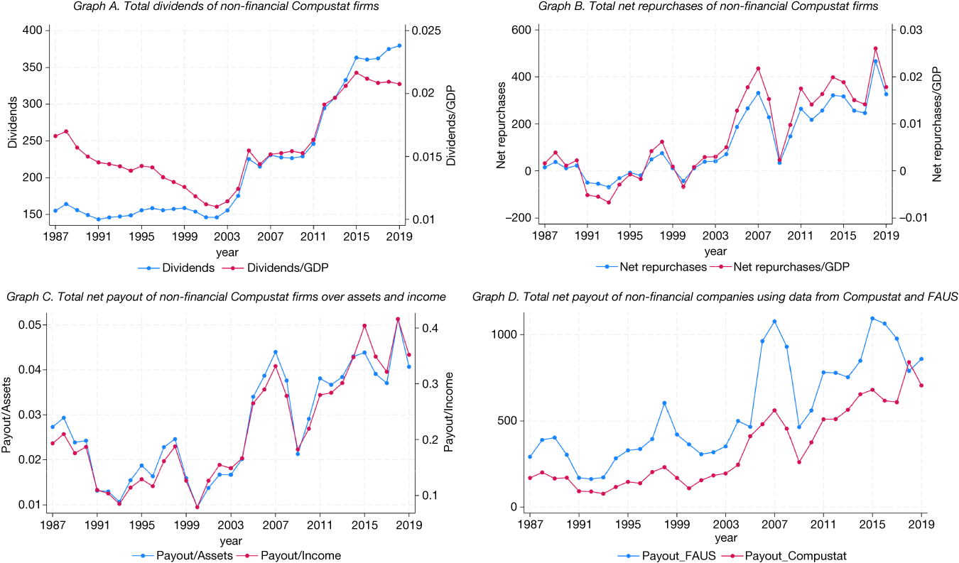

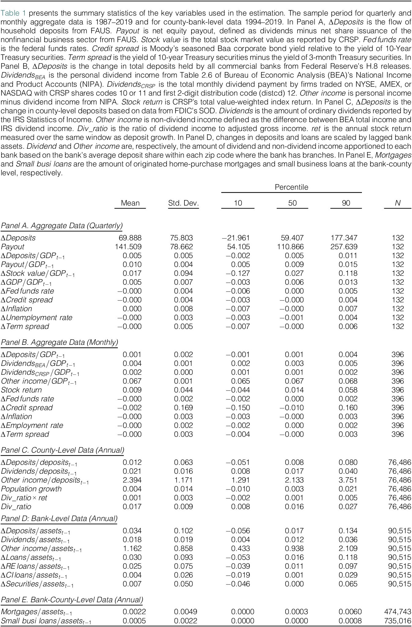
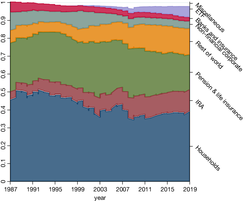

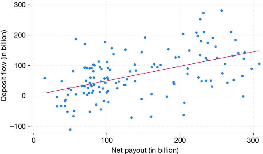

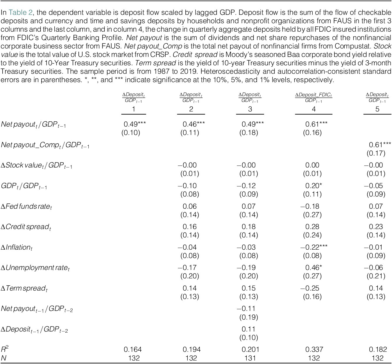
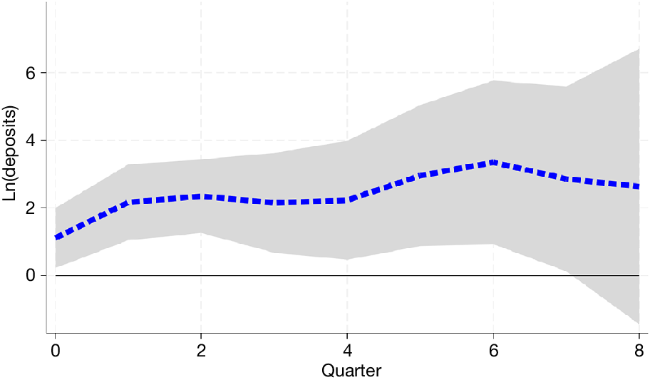


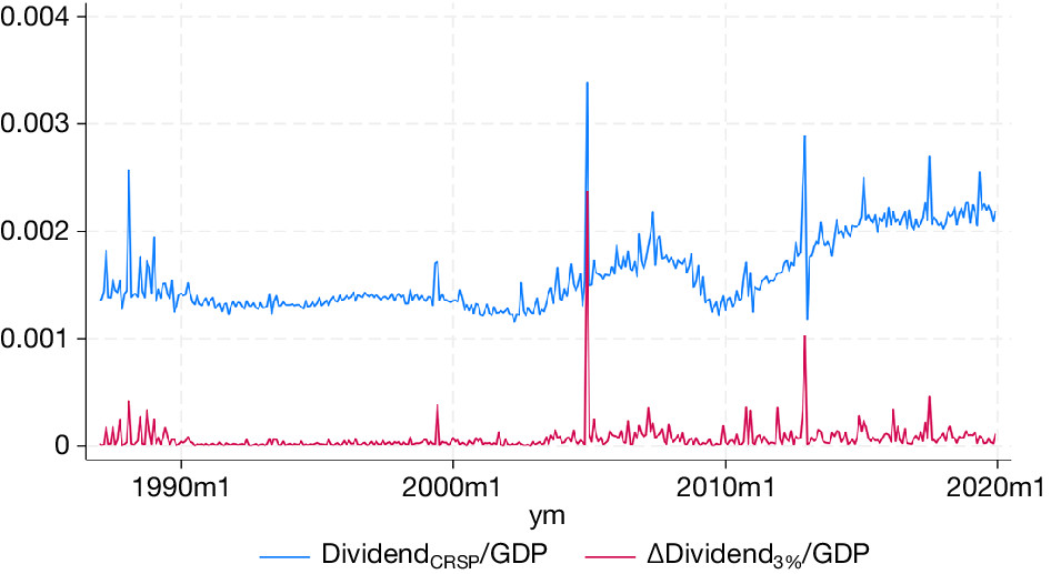


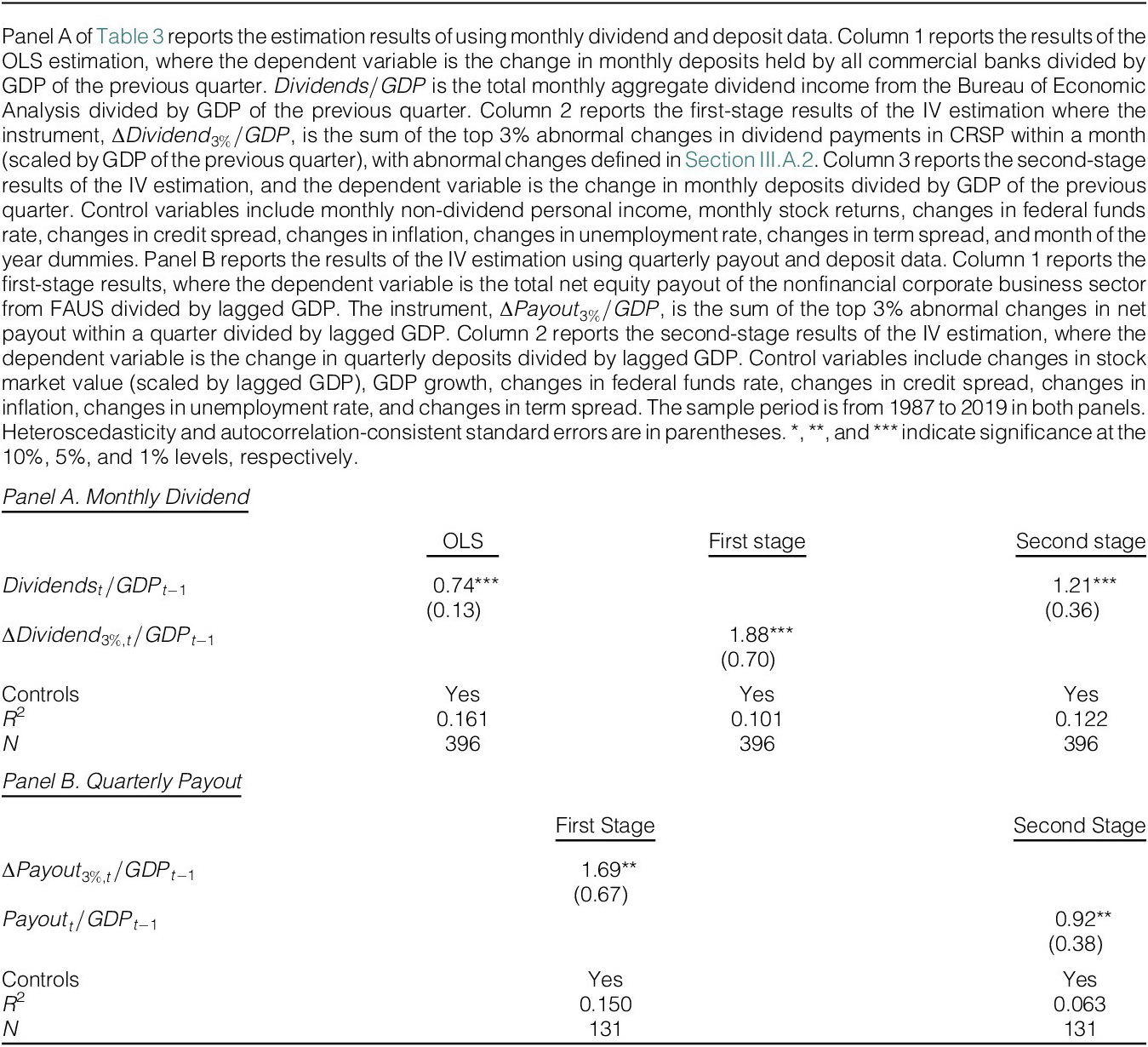
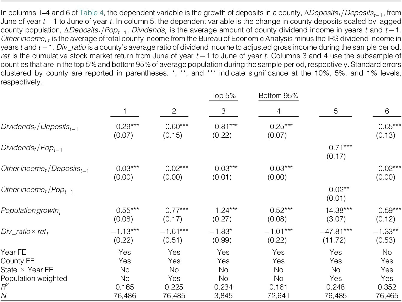
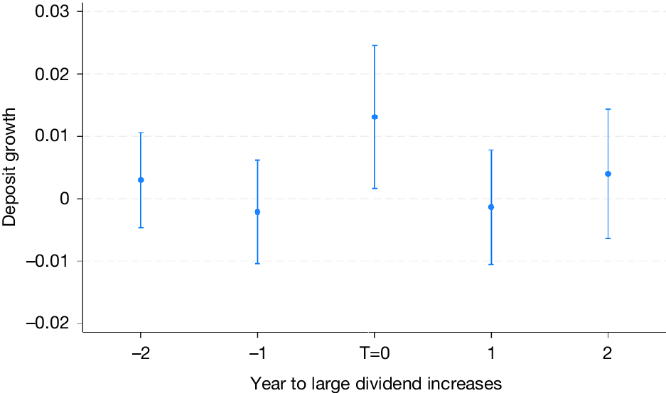

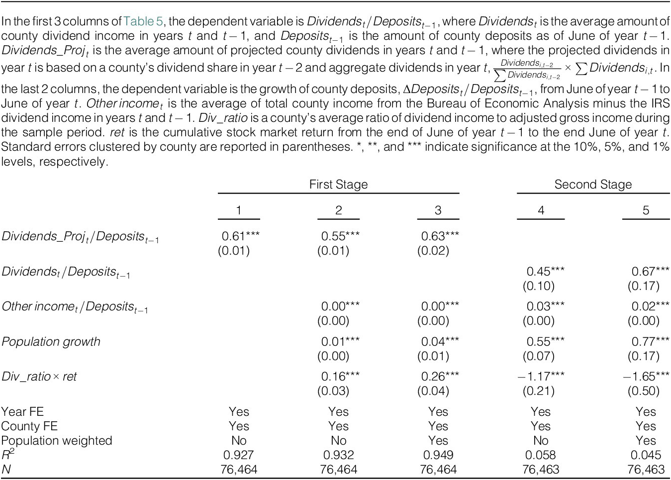
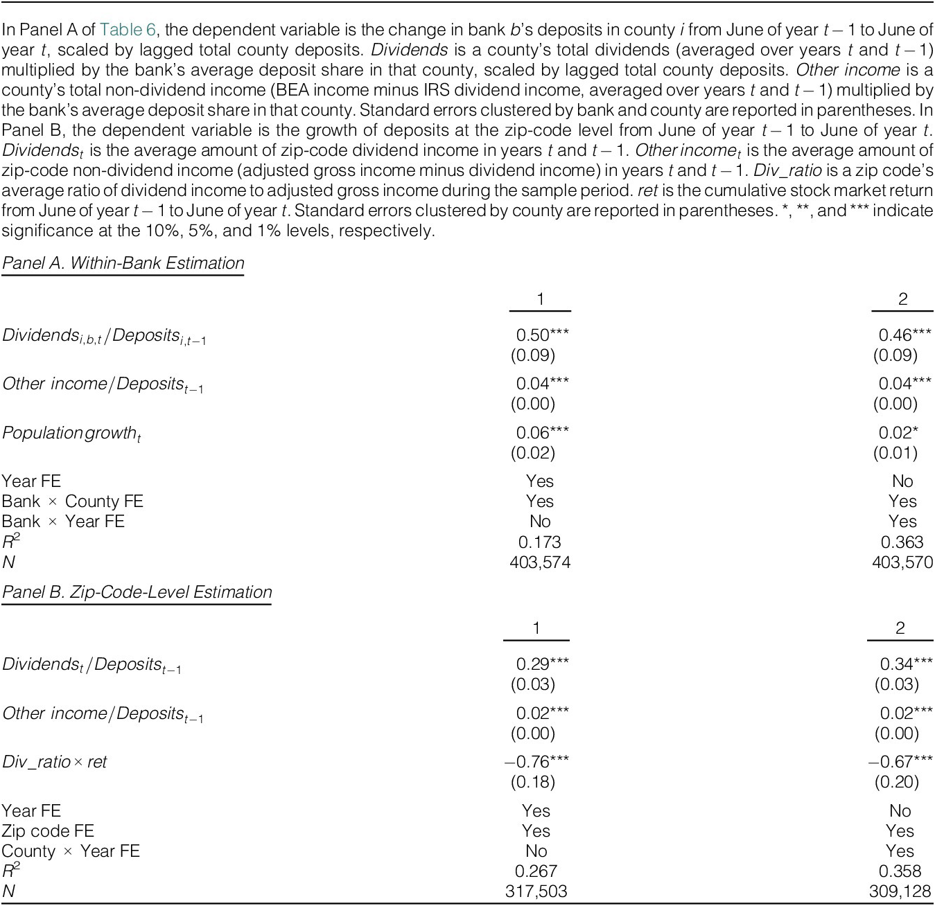
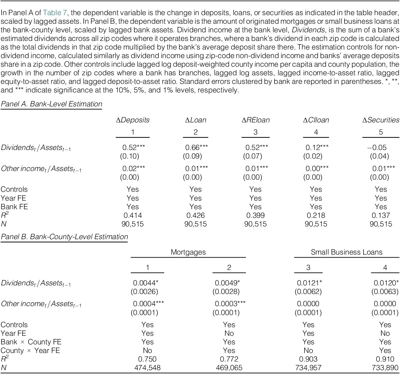


 Open access

