2.1. Wind tunnel facility and swept-wing model

The experimental measurements in this work are performed on the swept-wing model $66018M3J$ in the Low Turbulence Tunnel at Delft University of Technology. The $M3J$ model is extensively used in related experiments by the authors’ research group and is elaborately described by Serpieri & Kotsonis (Reference Serpieri and Kotsonis2015). Owing to the geometry design and sweep angle ($\varLambda =45^{\circ }$), the $M3J$ model is characterised by extensively favourable pressure gradients on the pressure side, favouring the growth of CFIs. Previous measurements at similar velocity conditions quantified the free-stream turbulence level of the Low Turbulence Tunnel to be $T_{u}<0.03\,\%$ (Serpieri Reference Serpieri2018), which guarantees the dominance of stationary CFIs (Bippes Reference Bippes1999).

Measurements are performed at various angles of attack $\alpha$ and various global $Re$, for which the flow approximately attains infinite swept-wing conditions. Figure 1(a) illustrates the $M3J$ geometry (in the $x$ axis) and a representative pressure coefficient $C_{p}$ distribution under conditions of $\alpha =2.5^{\circ }$ and $Re=2.5\times 10^{6}$. The pressure distributions are measured by the top and bottom pressure tap arrays, illustrated by red and blue dashed lines in figure 1(b). The similarity of the two pressure coefficients confirms the attainment of spanwise-invariant conditions. Two coordinate reference systems are used in this work, namely the tunnel-aligned $XYZ$ system and the wing-aligned $xyz$ system, as denoted in figure 1(b). It should be noted that the $y$ axis is body-fitted and aligns with the wall-normal direction of the local wing surface. The airfoil chords in directions of $X$ and $x$ are denoted as $c_X$ and $c_x$, respectively. The velocity vectors corresponding to the two coordinate systems are denoted as $[UVW]$ and $[uvw]$, respectively.

For the entirety of this work, non-dimensional quantities are denoted by the overbar symbol. In § 3, the numerical velocity quantities are non-dimensionalised by the free-stream velocity $u_\infty$ corresponding to $Re=2.5\times 10^6$. Whereas in § 4, various $Re$ cases are considered ($2.5\times 10^6$–$3.7\times 10^6$). Therefore, the PIV-measured velocity components for various $Re$ cases are non-dimensionalised by the corresponding free-stream velocity $U_\infty$. The spanwise distance $z$ and wall-normal distance $y$ are non-dimensionalised by the global reference length $\delta _0$. Specifically, $\delta _0$ is the Blasius length scale identified in the simplified model of § 3. Parameter $\delta _0$ is calculated as $\delta _0=\sqrt {\nu s_0/u_0}$, where $u_0$ is the boundary layer edge velocity at $x/c_x=0.0083$ (the calculation starting point). Viscosity $\nu$ refers to the air kinematic viscosity and $s_0$ is the surface distance from the stagnation point to $x/c_x=0.0083$. The scaling parameters used in the numerical calculation in § 3 are summarised in table 1. To facilitate the discussion, the terms plasma-off and plasma-on are used to refer to scenarios where PA is not activated and activated, respectively. The quantities at conditions of plasma-off and plasma-on are distinguished by the subscripts ‘off’ and ‘on’, respectively.

Table 1.

Scaling parameters pertaining to numerical base flow simulations ($\alpha =2.5^{\circ }$).

2.2. Stationary CFI conditioning and PA

As described in the introduction, swept-wing boundary layers are essentially dominated by stationary CFIs in realistic flight circumstances, due to the extremely low free-stream turbulence intensity $T_{u}$. In order to elucidate the BFM effects on such flow, the existence and development of stationary CFIs are required in the boundary layer. To this goal, two types of surface roughness arrays are designed and manufactured to enhance stationary CFIs. Specifically, a distributed roughness patch (DRP) is used to trigger a broad spectrum of stationary CFIs, appearing in non-deterministic spanwise wavelengths. The DRP is simply formed by layers of spray-on adhesive, which enhances the wing surface roughness through the random deposition of adhesive particles. To confine the spatial extend of the DRP, a rectangular PVC mask is used. 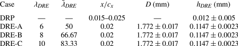Ultimately, the DRP is generated parallel to the leading edge, spanning from $x/c_x = 0.015$ to 0.025.

In contrast, for triggering deterministic, single-wavelength modes, arrays of DREs are used. Several DRE arrays of various spanwise spacings (i.e. $\lambda _{DRE}=6$, 8 and 10 mm) are designed and fabricated in-house. A computer-controlled laser cutting machine is used to shape self-adhesive black PVC foil with thickness of $100\,\mathrm {\mu } {\rm m}$. Each DRE array is installed at $x/c_{x}=0.02$, just upstream of the neutral point of the forced modes. For the same material and fabrication procedure, a shape characterisation of the fabricated DRP and DREs is described in the work of Zoppini et al. (Reference Zoppini, Michelis, Ragni and Kotsonis2022a,Reference Zoppini, Westerbeek, Ragni and Kotsonisb). The reported geometrical parameters of DRP and DREs are summarised in table 2. Hereafter, the symbols $\lambda _6$, $\lambda _8$ and $\lambda _{10}$ refer to the dimensional wavelengths of 6, 8 and 10 mm. These wavelengths are non-dimensionalised by $\delta _{0}$, resulting in $\bar {\lambda }_6=50$, $\bar {\lambda }_8=66.67$ and $\bar {\lambda }_{10}=83.33$.

Table 2.

Geometric parameters and chord locations of roughness arrays.

To enable plasma-based BFM, a two-dimensional spanwise-invariant DBD PA is utilised, similar to the type used by Yadala et al. (Reference Yadala, Hehner, Serpieri, Benard, Dörr, Kloker and Kotsonis2018a) and Peng et al. (Reference Peng, Arkesteijn, Avallone and Kotsonis2022a). The PA is fabricated using an automated metal deposition technique developed in-house, where electrodes are printed by sub-micrometric conductive silver spray. The resulting PA electrodes feature a thickness of a few micrometres, imposing negligible roughness effects on the boundary layer (Serpieri et al. Reference Serpieri, Venkata and Kotsonis2017; Yadala et al. Reference Yadala, Hehner, Serpieri, Benard, Dörr, Kloker and Kotsonis2018a). Both exposed and encapsulated electrodes feature a streamwise width (i.e. along the $x$ direction) of 5 mm with no gap between each other. Specifically, the encapsulated electrode is configured upstream of the exposed electrode with the interface located at $x/c_{x}=0.035$. Following the BFM control principle, the encapsulated electrode is connected to the ground and the exposed electrode is connected to the high-voltage signal, thus generating a body force vector largely oriented in the $-x$ direction, counteracting the CF component. A polyethylene terephthalate foil with a thickness of $500\,\mathrm {\mu } {\rm m}$ is used as the dielectric material, which is further wrapped around the wing leading edge and extends downstream to avoid potential surface irregularities. For the entirety of this work, the PA is powered by a GBS Electronik Minipuls 4 high-voltage amplifier, where the actuation frequency $f_{AC}$ is set at 12.5 kHz. Though the supplied voltage $V_{p-p}$ is set at 7 kV for the body force characterisation experiment (§ 3), $V_{p-p}$ is set at 6.5 kV for subsequent IR and PIV measurements in the wind tunnel (§§ 4 and 5). This choice is aimed at mitigating electrode degradation resulting from lengthy operation during measurements. Nonetheless, this small difference in $V_{p-p}$ is assumed to minimally affect the PA forcing strength and spatial distribution, allowing for a qualitative reflection of the physics underlying the experimental findings.

2.3. Planar PIV

Velocity vector fields are extracted by planar PIV for various $Re$ conditions while the $M3J$ model is set at $\alpha =2.5^{\circ }$. Micrometre-diameter seeding particles are illuminated by a Quantel Evergreen Nd:YAG dual-cavity laser (200 mJ at a wavelength of 532 nm), providing a laser sheet aligned to the $yz$ plane at $x/c_{x}=0.175$. Per test case, one LaVision imager camera (sCMOS, $2560\,{\rm px} \times 2160\,{\rm px}$) acquires 600 image pairs at a sampling frequency of 15 Hz. For the various $Re$ cases, the inter-frame time interval of image pairs is appropriately adjusted such that the free-stream particle displacement is around 12 pixels. Particle images are further processed in LaVision Davis 10 through the cross-correlation to obtain the velocity vector $[vw]$. Each image pair is processed through a multi-pass cross-correlation algorithm with a final interrogation window of $12\,{\rm px} \times 12\,{\rm px}$ and 50 % overlap. The average flow field is constructed as the average of 600 instantaneous PIV vector fields. Considering laser light reflections and significant velocity uncertainty near the wall, the velocity vectors in that region ($y<0.3\,{\rm mm}$) are discarded in subsequent analyses due to the low reliability. Additionally, $y_{min}$ refers to $y=0.3\,{\rm mm}$ for the entirety of the work. The case of DRE-A at $Re=3.7\times 10^{6}$, which is anticipated to have the highest level of velocity uncertainty, is used to compute the time-averaged uncertainty. As a consequence, the maximum uncertainty for $w$ is found as $0.5\,\%U_{\infty }$ in the boundary layer region, while the average uncertainty is identified as $0.012\,\%U_{\infty }$ in the free-stream region. Additionally, the combinations of tested $Re$ and $\alpha$ for PIV as well as IR measurements are summarised in table 3.

Table 3.

Reynolds number $Re$ and $\alpha$ combinations for PIV and IR measurements.

2.4. Infrared thermography

According to the Reynolds analogy, in boundary layer flows the rate of heat convection is a direct function of local wall shear stress. As such, for a given heat flux, variations in shear stress will result in surface temperature differences, which can be identified through IR thermography. This non-intrusive technique is extensively used in associated studies by the authors’ research group, which has been proven as expeditious in visualising the thermal footprint of stationary CF vortices and the resulting laminar–turbulent transition front (Rius-Vidales & Kotsonis Reference Rius-Vidales and Kotsonis2020; Zoppini et al. Reference Zoppini, Westerbeek, Ragni and Kotsonis2022b).

In the current experiment, two Optris PI640 IR cameras ($640\,{\rm px} \times 480\,{\rm px}$, NETID 75 mK) are utilised to measure the wing surface temperature. The first camera coupled with a wide-angle lens ($\,f_\#=10.5\,{\rm mm}$) is designated as IR-Full and captures the entire wing surface temperature. The second camera, named IR-Zoom, is coupled with a telephoto lens ($\,f_\#=41.5\,{\rm mm}$), imaging a small region in the middle of the wing (domain outlined by the magenta box of figure 2a, from $x/c_{x}=0.0565$ to 0.2385). Approximately 40 images are recorded by these cameras for each run at a sampling frequency $f_s=4\,{\rm Hz}$, which are later time-averaged to reduce background noise. Additionally, several halogen lamps are used to radiate the wing model in order to improve the thermal contrast.

Figure 2.

Time-average IR images of transition front visualisation (DRE-B, $\alpha =2.5^{\circ }$ and $Re=3.3\times 10^{6}$) for (a) PA-off and (b) PA-on. Flow comes from the left and the leading edge is shown by the black line. The PA location is indicated by red dashed line. (c) Subtraction of IR image of (a,b). Gained laminar flow (magenta) and lost laminar flow (cyan). (d) Simple sketch for clarifying the transformation between the net laminar gain and transition location shift (not to scale).

Typical time-average IR images of the transition front are shown in figure 2(a,b). Specifically, the turbulent region presents darker tone while the laminar region shows brighter tone. Figure 2(c) illustrates the IR intensity subtraction $\Delta I$ between panels (a) and (b). The white area (near the transition front) corresponds to the gained laminar flow (i.e. transition delay) and the black area corresponds to the gained turbulent flow (transition advance). For this work, the gained laminar area $s_l$ can be roughly identified as regions of $\Delta I>\Delta I_r$ while the lost laminar area $s_t$ is identified as regions of $\Delta I<-\Delta I_r$, where $\Delta I_r$ is a threshold value. Variations of the threshold value are tested in order to identify the sensitivity of gained and lost laminar flow areas. Reasonable areas of gained and lost laminar flow can be identified with a threshold between 0.3 and 0.6. As a result, $\Delta I_r=0.4$ is chosen as the threshold for the subsequent processing. Though the threshold of 0.4 is chosen heuristically, it remains constant for the entire parameter range to produce comparable outcomes. Typical results of $s_l$ and $s_t$ are given in figure 2(c), outlined by the magenta and cyan lines, respectively (at the threshold of 0.4). Consequently, the net laminar gain is calculated as $s_l-s_t$. The net laminar gain is further transformed to an equivalent transition location shift $\Delta (x_t/c_x)$ used in the discussion in § 5.2. Figure 2(d) depicts a simple sketch which aids in clarifying the transformation. Using the area rule of a parallelogram, an equivalent spanwise-invariant transition location shift is found as a function of the net laminar area gain, as shown by (2.1):

(2.1)\begin{equation} \frac{(s_l-s_t)}{\Delta (x_t/c_x)}=\frac{s_r}{(0.2-0.1)}=h , \end{equation}

where $s_r$ refers to the constant area between $x/c_{x}=0.1$ and 0.2 (blue area) and $h$ is the parallelogram height.

Beyond the identification of laminar gain or loss, the use of IR thermography also enables access to the nature of laminar breakdown. More specifically, the loss of spatial coherency in the transition front (i.e. ‘blurriness’) can be expected to underline a change between a stationary CFI and travelling CFI scenario (Downs & White Reference Downs and White2013; Borodulin, Ivanov & Kachanov Reference Borodulin, Ivanov and Kachanov2015). As such it is desirable to formalise and quantify this effect. In the field of image processing, a blurred object is characterised by a gradual variation in intensity scale (e.g. IR intensity $I$ in this paper) along its outline when compared with a sharp object. In the context of this work, the object is the wedged transition front where a blurred wedge edge is expected to exhibit a relatively smaller gradient compared to a sharp edge. Consequently, the detection of transition front blurriness can be facilitated by simply quantifying the IR intensity gradient at edges of transitional wedges. For all tested cases, the general trend of the transition front follows an angle of $45^{\circ }$ with the $X$ axis, highlighting the importance of both $x$ gradient and $y$ gradient of $I$. As a result, the intensity gradient $|\boldsymbol {\nabla } I|=\sqrt {|{\partial I}/{\partial x}|^2+|{\partial I}/{\partial y}|^2}$ is calculated for all cases and representative results are displayed in figure 3(b,e). In general, plasma-off cases result in intensified $|\boldsymbol {\nabla } I|$ values outlining the typical wedged transition front, while plasma-on cases result in minimal $|\boldsymbol {\nabla } I|$ due to the blurred transition front. Similar results of $|\boldsymbol {\nabla } I|$ are found for the majority of tested cases (not shown here for brevity), demonstrating the efficacy of $|\boldsymbol {\nabla } I|$ as an indication of the transition front blurriness. The intensity gradient $|\boldsymbol {\nabla } I|$ is only considered in a mask region (outlined by magenta lines as shown in figure 3) to exclude the strong gradient caused by the PA. Within this mask region, the paper focuses on the $|\boldsymbol {\nabla } I|$ of sufficiently strong values ($|\boldsymbol {\nabla } I|>0.25$) to effectively eliminate background noise. The filtered $|\boldsymbol {\nabla } I|$ is illustrated in figure 3(c,f). In the context of this work, the $|\boldsymbol {\nabla } I|$ is employed solely as a means to reflect the plasma-caused alteration of transition front blurriness. Through a batch of tests, any threshold value between 0.2 and 0.28 is deemed appropriate for this goal. In this paper, the threshold is arbitrarily chosen as 0.25 and maintained consistently throughout the entire processing, ensuring comparable results. Consequently, the average density of $|\boldsymbol {\nabla } I|$ is identified as $|\boldsymbol {\nabla } I|_{d}=\varSigma |\boldsymbol {\nabla } I|/s_I$, where $s_I$ is the mask area outlined by the magenta lines and $\varSigma |\boldsymbol {\nabla } I|$ refers to the sum of $|\boldsymbol {\nabla } I|$ in the mask region.

Figure 3.

Transition front identification under $Re=2.5\times 10^6$ and $\alpha =2.5^{\circ }$ (DRE-B). (a,d) Time-average IR images; (b,e) IR intensity gradient $|\boldsymbol {\nabla } I|$; (c,f) filtered IR intensity gradient ($|\boldsymbol {\nabla } I|>0.25$).

4.1. Stationary CFIs

Figure 7(a) illustrates the time-average velocity field $\bar {w}$ (contour) and spanwise gradient $\partial \bar {w} /\partial \bar {z}$ (colour) in the case of $Re=2.5\times 10^{6}$. Among all tested cases, DRP induces the least significant stationary flow perturbation, presenting a scenario of weakly amplified stationary CFI modes. In contrast, the mean flow fields of all DRE cases show evident spanwise-periodic modulations, presenting scenarios where stationary CFI modes are significantly enhanced. Among all the DRE cases, DRE-A produces considerably more amplified and coherent stationary vortices. This is in agreement with the preliminary LST predictions which suggest that stationary CFI modes of smaller $\lambda$ obtain larger $N$ factors in the vicinity of the leading edge.

Figure 7.

Spanwise gradient $\partial \bar {w}/\partial \bar {z}$ (colour) at (a) $Re=2.5\times 10^{6}$ and (b) $Re=3.7\times 10^{6}$. Measurements are taken for DRP, DRE-A, DRE-B and DRE-C (columns from left to right) at $x/c_{x}= 0.175$. Black iso-lines illustrate the time-average velocity $\bar {w}$, five levels from 0 to 0.7.

In all DRE cases the flow fields undergo evident changes when the PA starts working. Noticeably, the PA operation shifts the location of stationary CF vortices towards the $+z$ direction (i.e. more aligned with the outer inviscid streamlines). This spanwise shift of CF vortices appears as a typical outcome of the BFM strategy, attributed to the localised reduction of the CF component (Peng et al. Reference Peng, Arkesteijn, Avallone and Kotsonis2022a). More importantly, the local maximum and minimum of the spanwise velocity gradient $\partial \bar {w}/\partial \bar {z}$ are significantly weakened by the PA forcing, indicating a weakening of the stationary CF vortices. Similar observations are also found for cases at higher $Re=3.7\times 10^6$ (figure 7b). Alternatively, the reduction of stationary CFI modes is demonstrated and reflected by the degradation of stationary mode shape. The stationary mode shape is calculated as the spanwise standard deviation of $w$ and denoted as $\langle w \rangle _z$. The mode shape profiles are illustrated in figure 8 at $Re=2.5\times 10^6$ and $Re=3.7\times 10^6$. As expected, the spanwise modulation of stationary modes is integrally weakened by the PA forcing. In addition, the secondary hump on the perturbation profiles (denoted by the circular marker) is modified by the PA as well. This secondary hump is related to the characteristic lobe structure of stationary CFIs, which coincides with the advent of nonlinear interactions (Haynes & Reed Reference Haynes and Reed2000; White & Saric Reference White and Saric2005). In terms of the lowest-$Re$ cases (figure 8a), the secondary hump only occurs in DRE-A under the condition of plasma-off. This result indicates that stationary CFI modes of DRE-A develop fastest thus first reaching the nonlinear stage, demonstrating the importance of stationary mode receptivity. Considering that the lobe structure is commonly associated with stationary mode saturation and onset of secondary CFIs (Serpieri & Kotsonis Reference Serpieri and Kotsonis2016), the PA forcing appears to retard the evolution of stationary CFI modes.

Figure 8.

Standard deviation profiles of $\langle w \rangle _{z}$ at (a) $Re=2.5 \times 10^{6}$ and (b) $Re=3.7 \times 10^{6}$.

To better isolate the forced stationary CFI modes, the spanwise periodicity of the mean flow is leveraged through a spatial fast Fourier transform of the time-average velocity fields. Representative spatial spectra at $Re=2.5\times 10^{6}$ are illustrated in figure 9. For plasma-off, no significant spectral energy is observed in DRP while the $\bar {\lambda }_6$ and $\bar {\lambda }_8$ modes are evidently amplified in DRE-A and DRE-B, along with their harmonic modes. In spite of the successful excitation of stationary CFI modes corresponding to $\lambda _{DRE}$ in DRE-A and DRE-B, the opposite is observed in DRE-C. Instead of the $\bar {\lambda }_{10}$ mode, the $\bar {\lambda }_6$ mode is most enhanced by DRE-C, though weaker than that found in DRE-A. Additionally, multiple spectral modes are amplified which are not necessarily related to $\bar {\lambda }_{10}$ or its harmonics. The apparent inability of configuration DRE-C to trigger the respective wavelength of CFIs should be attributed to the fact that the $\bar {\lambda }_{6}$ mode is significantly more unstable than the $\bar {\lambda }_{10}$ mode at the upstream region of DRE forcing, as indicated by the LST results (figure 5). Notwithstanding, when the PA is on, these DRE-induced spectral modes including their harmonics are evidently inhibited. In contrast, the plasma forcing appears to increase the amplitude of stationary CFIs in the DRP case.

Figure 9.

Non-dimensional spectral amplitude $\bar {A}(\bar {\lambda })$ for (a) plasma-off and (b) plasma-on at $Re= 2.5\times 10^{6}$. Black filled triangle, $\bar {\lambda }=50\ (\lambda =6\,{\rm mm})$; black open triangle, $\bar {\lambda }=25\ (\lambda =3\,{\rm mm})$; red filled triangle, $\bar {\lambda }=66.67\ (\lambda =8\,{\rm mm})$; red open triangle, $\bar {\lambda }=33.33\ (\lambda =4\,{\rm mm})$; blue filled triangle, $\bar {\lambda }=83.33$ $(\lambda =10\,{\rm mm})$.

The spanwise wavelength spectra are further used to quantify the integral amplitude of stationary CFI modes. Specifically, the spectral energy of discrete Fourier modes is integrated from $\bar {y}_{min}$ to $\bar {y}=25$ (i.e. $y=3\,{\rm mm}$) and denoted as $\bar {A}_s(\bar {\lambda })$. Peaks at $\bar {\lambda }_{10}$, $\bar {\lambda }_6$, $\bar {\lambda }_8$ and $\bar {\lambda }_6$ are chosen as the dominant spectral modes for DRP, DRE-A, DRE-B and DRE-C, respectively. The results are illustrated in figure 10 at various $Re$. Overall, the plasma-based BFM leads to a suppression of stationary CFI modes for all DRE cases as also observed by Peng et al. (Reference Peng, Arkesteijn, Avallone and Kotsonis2022a). It is noticed that the modes around $\bar {\lambda }_{10}$ in DRP are slightly enhanced at lower $Re$ though further reduced with increasing $Re$. Though the origin of this amplification cannot be conclusively determined here, the slow variance or modulation of PA discharge along the spanwise direction appears as a potential cause, which can result from the possible misalignment in PA fabrication and placement. Nonetheless, these additional modes are expected to have insignificant effects on the transition dynamics due to their weak amplitudes. This holds particularly true for DRP cases at higher $Re$ and DRE cases where these additional modes are effectively suppressed by the strong dominant modes induced by the DREs.

Figure 10.

Non-dimensional amplitude $\bar {A}_{s}(\bar {\lambda })$ of dominant spectral modes for (a) DRP, (b) DRE-A, (c) DRE-B and (d) DRE-C.

4.2. Travelling CFIs

The amplitude reduction of stationary CFI modes underlines the positive effects of plasma-based BFM on stabilising the boundary layer. Notwithstanding, previous studies of Serpieri et al. (Reference Serpieri, Venkata and Kotsonis2017) and Peng et al. (Reference Peng, Arkesteijn, Avallone and Kotsonis2022a) have shown that the PA operation inevitably induces travelling CFIs in the boundary layer, which might be attributed to quasi-stochastic processes within the PA micro-discharge (Moralev et al. Reference Moralev, Selivonin and Ustinov2019). Furthermore, the previous LST results indicate that the net BFM effect favours the suppression of stationary over travelling CFI modes, essentially rendering the boundary layer more susceptible to travelling CFIs. In combination, these factors highlight the significance of travelling CFI modes in realistic applications of plasma-based BFM, adding complexity to the successful implementation of this method.

Figure 11 illustrates the unsteady velocity fluctuation $\langle \bar {w}^{\prime } \rangle$ (colour) overlaid with time-average velocity (contour) at $Re=2.5\times 10^{6}$ and $Re=3.7\times 10^{6}$. At the condition of $Re=2.5\times 10^{6}$ and plasma-off, unsteady fluctuations already become non-negligible in the near-wall region within the stationary vortex structures. Compared with the DRP case, the unsteady fluctuations are evidently more spanwise-periodic in DRE cases due to the stronger modulation of stationary CFI modes. Among all DRE cases, the intensified unsteady fluctuations are more centralised and compact in DRE-A, corresponding to the highly amplified state of the stationary vortices in this case. Recalling figure 8(a), the level of unsteady fluctuations further demonstrates that the primary CFIs of DRE-A are at a nonlinear stage of growth and subject to a strong mutual interaction at $Re=2.5\times 10^{6}$ and $x/c_{x}=0.175$. In contrast, the primary CFIs in DRE-B and DRE-C cases reveal a weaker mutual interaction. When the PA is on, the plasma forcing evidently amplifies unsteady fluctuations in the DRP case, resulting in a boundary layer significantly contaminated by travelling CFIs. In contrast, the PA forcing appears to only marginally affect the DRE cases. In these cases, the spanwise-modulated fluctuations become weaker centrally and tend to spread spatially within stationary structures. Similar results are observed at $Re=3.7\times 10^{6}$, though the unsteady fluctuations exhibit higher amplitudes and more pronounced modulation in the spanwise direction for both plasma-off and plasma-on.

Figure 11.

Non-dimensional standard deviation of temporal velocity fluctuation $\langle \bar {w}^{\prime } \rangle$ for (a) $Re=2.5\times 10^6$ and (b) $Re=3.7\times 10^6$. The colourbar follows a logarithmic scale.

These unsteady fluctuations are mainly amplified in regions of strong spanwise gradients, as shown in figure 7. The spatial locations of these unsteady fluctuations highly resemble the primary type III mode and the secondary type I mode (Wassermann & Kloker Reference Wassermann and Kloker2002). However, these typical fluctuations cannot be conclusively segregated here considering the low acquisition frequency of the utilised PIV measurement technique. Nonetheless, these fluctuations are carefully examined given their intrinsic associations with type III and type I modes, as well as the mutual interactions of primary CFI modes. Hereafter, the fluctuations corresponding to the minimum $\partial \bar {w}/ \partial \bar {z}$ and the maximum $\partial \bar {w}/ \partial \bar {z}$ are denoted as fluctuation-a and fluctuation-b, as outlined by the red and black lines in figures 7(b) and 11(b). These fluctuation structures are quantified following the method in Peng et al. (Reference Peng, Avallone and Kotsonis2022b), where the fluctuation $\langle \bar {w}^{\prime } \rangle$ is integrated within specific spatial regions (i.e. masks). Specifically, the region of $\partial \bar {w}/ \partial \bar {z}<-0.5\max (\partial \bar {w}/ \partial \bar {z})$ is used to trace fluctuation-a structure and the region of $\partial \bar {w}/ \partial \bar {z}>0.5\max (\partial \bar {w}/ \partial \bar {z})$ for fluctuation-b structure. While the threshold of 0.5 is chosen heuristically, it is kept constant for the entire parameter range, ensuring comparable outcomes. The amplitudes of the two fluctuation structures are ultimately calculated as follows:

(4.1)\begin{equation} \bar{A}_i= \frac{1}{s_{m,i}} \int\int_{s} \langle \bar{w}^{\prime} \rangle \,{\rm d} s, \end{equation}

where $i=a,b$ and $s_m$ denotes the mask area.

The resulting amplitudes $\bar {A}_a$ and $\bar {A}_b$ are illustrated in figures 12(a) and 12(b), respectively. In accordance with the observations in figure 11, the amplitudes of fluctuation-a and fluctuation-b structures are significantly reduced by the PA forcing for all DRP and DRE cases. To facilitate the discussion, the total unsteady fluctuations and stationary CFIs are further quantified. Specifically, the total unsteady fluctuations over the entire domain are quantified as follows: (Downs & White Reference Downs and White2013)

(4.2)\begin{equation} \bar{A}_t= \frac{1}{\delta_{99}-y_{min}}\frac{1}{z_{max}} \int_{0}^{z_{max}}\int_{y_{min}}^{\delta_{99}}\langle \bar{w}^{\prime} \rangle \,{\rm d} z\,{\rm d} y, \end{equation}

where $z_{max}$ is the spanwise extent of the PIV domain (figure 11) and $y_{min}$ is the nearest to the wall position, reliably resolved by the PIV measurement (§ 2.3). The results are summarised in figure 12(c), revealing a general amplification of travelling CFIs due to the PA forcing in all DRP and DRE cases. Though the LST results in § 3 indicate that the net BFM effect essentially weakens both types of CFIs, the impact of intrinsic non-deterministic unsteadiness of the PA forcing results in a relatively more amplified $\bar {A}_t$. Additionally, it is not surprising to find that $\bar {A}_t$ displays an opposing tendency compared with $\bar {A}_a$ and $\bar {A}_b$ when the PA is on. This is due to the fact that unsteady fluctuations are mildly amplified by the PA outside of the region of structures a and b (typically evident in DRP cases) and are accumulatively reflected by $\bar {A}_t$. Furthermore, the amplitudes of total stationary CFI modes $\bar {A}_{s}$ are simply calculated as the integral of spanwise standard deviation of $\langle \bar {w} \rangle _{z}$ as follows:

(4.3)\begin{equation} \bar{A}_s=\frac{1}{\delta_{99}-y_{min}}\int_{y_{min}}^{\delta_{99}} \langle \bar{w} \rangle_{z} \,{{\rm d}y} . \end{equation}

The results are shown in figure 12(d). As expected, the amplitudes of total stationary modes agree well with the dominant mode amplitudes $\bar {A}_s(\bar {\lambda })$ as shown in figure 10, indicating a general reduction of stationary CFI modes due to plasma forcing.

Figure 12.

(a) Fluctuation-a amplitude $\bar {A}_a$. (b) Fluctuation-b amplitude $\bar {A}_b$. (c) Unsteady fluctuation amplitude $\bar {A}_t$. (d) Stationary CF mode amplitude $\bar {A}_s$. (e) Ratio $\bar {A}_t/\bar {A}_s$. The vertical coordinates follow a logarithmic scale.

It should be noted that the observed reduction of fluctuation-a and fluctuation-b structures is not contradictory to the observations of Peng et al. (Reference Peng, Arkesteijn, Avallone and Kotsonis2022a), where they were found to be significantly amplified in cases of strongly nonlinear stationary CFIs (i.e. larger $h_{DRE}$). In fact, the increase of $\bar {A}_t$ and the decrease of $\bar {A}_s$ imply that the reduction of fluctuation-a and fluctuation-b structures can be attributed to the significantly weakened stationary CFI modes. Ultimately, fluctuation-a and fluctuation-b structures tend to depend on the amplitude of their carrying stationary CFI modes remaining downstream of the PA forcing region. This assumption is further supported, considering that stationary CFI modes are significantly weakened by the PA in the present study while remaining almost unaffected in the nonlinear cases of Peng et al. (Reference Peng, Arkesteijn, Avallone and Kotsonis2022a).

Considering the above observations, two primary outcomes governing the response of stationary and travelling CFI modes to the PA forcing can be extracted. The first scenario occurs when the net BFM effect takes dominance, leading to the suppression of both types of CFI modes, as usually found in numerical studies (Dörr & Kloker Reference Dörr and Kloker2015; Guo & Kloker Reference Guo and Kloker2019). Comparatively, the stationary CFI modes tend to be more suppressed in this case, as implied by the LST results. Alternatively, the second scenario arises when the intrinsic non-deterministic unsteadiness of the PA outweighs the net BFM effect, resulting in a significant amplification of travelling CFI modes along with the suppression of stationary CFI modes, as demonstrated in the present study. Notwithstanding, in either scenario, the influences of travelling CFI modes in the boundary layer are expected to be enhanced due to the PA forcing. To estimate such influence, the ratio $\bar {A}_{t}/\bar {A}_{s}$ is calculated and illustrated in figure 12(e). The ratio $\bar {A}_{t}/\bar {A}_{s}$ significantly increases at plasma-on conditions. Nonetheless, it should be noted that this ratio $\bar {A}_{t}/\bar {A}_{s}$ is a more appropriate metric for linear cases (i.e. cases at relatively low $Re$) where nonlinear CFI modes (e.g. type III and secondary CFI modes) are not significantly amplified. Furthermore, $\bar {A}_{t}/\bar {A}_{s}$ differs significantly from $N^{env}_{t}/N^{env}_{s}$ discussed in § 3 and no direct comparison can be drawn at this point.

5.1. Transition topology

Figure 13 illustrates time-average IR images for DRP, DRE-A, DRE-B and DRE-C at $Re=2.5\times 10^6$. The leading edge of the $M3J$ model is indicated by the white solid line, while the red dashed line indicates the PA location. Additionally, blue dashed lines correspond to constant chord locations $x/c_{x}=0.1$, 0.2, 0.3 and 0.4. For plasma-off, contiguous turbulent wedges appear along the wing span for all tested cases, visualised by the thermal footprint caused by the local breakdown of stationary CF vortices (Saric et al. Reference Saric, Reed and White2003). These wedged transition fronts are also widely observed in swept-wing transition studies (Saric et al. Reference Saric, West, Tufts and Reed2019; Rius-Vidales & Kotsonis Reference Rius-Vidales and Kotsonis2020) and offer a first indication of the dominance of stationary CFIs at plasma-off conditions. In fact, stationary CFI-dominated boundary layers are expected at plasma-off conditions, considering the low level of free-stream turbulence $T_u$ (${<}0.03\,\%$) in the Low Turbulence Tunnel facility and the sensitivity of stationary CFIs to surface roughness (i.e. DRP or DREs). Nonetheless, these wedged transition topologies feature distinct differences between DRP- and DRE-conditioned cases. Evidently, DREs create more spanwise uniform transition fronts than DRP, due to the former's ability to concentrate perturbation energy in one single instability mode (Saric et al. Reference Saric, Reed and White2003; Zoppini et al. Reference Zoppini, Michelis, Ragni and Kotsonis2023). In contrast, the distributed and broadband nature of DRP results in a more irregular transition pattern.

Figure 13.

Transition front visualisation at $\alpha =2.5^{\circ }$ and $Re=2.5\times 10^{6}$ for (a) plasma-off and (b) plasma-on. Flow comes from the left and measurements are taken for DRP, DRE-A, DRE-B and DRE-C (columns from left to right).

The characteristics of stationary CFI modes at plasma-off are further revealed by the spanwise wavelength spectra of IR imaging fields, as illustrated in figure 14(a). These spectra are extracted from images of camera IR-Zoom, imaging a FOV corresponding to the magenta box region in figure 13. The absence of evident spectral modes in the upstream portion of the FOV indicates no single monochromatic stationary CFI mode triggered by DRP, agreeing well with the previous PIV observations. In contrast, evident energy peaks are found at $\bar {\lambda }_6$ and $\bar {\lambda }_8$ respectively for DRE-A and DRE-B, confirming the upstream DRE excitation. Despite the same roughness element height $h_{DRE}$ of DRE-A and DRE-B (i.e. similar initial amplitudes of $\bar {\lambda }_6$ and $\bar {\lambda }_8$ modes), the stationary CF mode of $\bar {\lambda }_6$ shows an earlier growth than that of $\bar {\lambda }_8$ at both low and high $Re$. This is also in agreement with the LST prediction, namely stationary modes of smaller wavelength are more amplified in the upstream region of the flow. Consistent with the PIV observations, instead of the $\bar {\lambda }_{10}$ mode, the $\bar {\lambda }_6$ mode is evidently amplified upstream, indicating the dominance of the $\bar {\lambda }_6$ mode in DRE-C, though weaker than those induced by DRE-A. In fact, besides the LST-predicted early amplification of stationary modes of shorter $\bar {\lambda }$, the triggering of the $\bar {\lambda }_6$ mode could be potentially attributed to the distinct neutral point locations of $\bar {\lambda }_6$ and $\bar {\lambda }_{10}$. As shown in figure 5(b), the neutral point of $\bar {\lambda }_{10}$ is significantly downstream from the DRE location (i.e. $x/c_x=0.02$) compared with $\bar {\lambda }_{6}$, which may consequently hinder the effective excitation of the $\bar {\lambda }_{10}$ mode in the DRE-C case.

Figure 14.

Wavelength spectra of the same cases as in figure 13. Blue dashed lines correspond to $x/c_{x}=0.1$ and 0.2. The black, red and blue triangles indicate wavelengths $\bar {\lambda }_6$, $\bar {\lambda }_8$ and $\bar {\lambda }_{10}$, respectively.

Figure 14(b) presents the wavelength spectra for plasma-on. The spectra demonstrate that the PA forcing weakens the DRE-induced spectral peaks, confirming the general effect of plasma-based BFM in attenuating stationary CFI modes and agreeing well with previous PIV results. Despite the presence of weaker stationary CFI modes in plasma-on scenarios, the ensuing transition front is expected to be topologically similar to that of the plasma-off case (i.e. sharp transition front), as long as stationary CFI modes are still dominant. However, a noticeable change in transition front topology is shown in figure 13(b) and indicates that plasma-based BFM does more than just weakening stationary CFI modes. Compared with plasma-off cases, the PA operation imposes a ‘blurring’ effect on the transition front, where distinct turbulent wedges are spatially spread or even eradicated. This distinct blurred transition front is commonly attributed to the rise of travelling CFI modes and their subsequent unsteady laminar breakdown (Downs & White Reference Downs and White2013). Unlike stationary CFI modes that predominantly propagate along local streamlines, travelling CFI modes exhibit significant deviations in the propagation direction with respect to local streamlines. This observation indicates the enhanced involvement of travelling CFI modes in the boundary layer development and transition process, due to the PA operation.

Following the method introduced in § 2.4, the IR intensity gradient density $|\boldsymbol {\nabla } I|_{d}$ is used to quantify the blurriness of the transition front, as illustrated in figure 15. Additionally, the ratio $c_{I}$ defined as $(|\boldsymbol {\nabla } I|_{d,off}-|\boldsymbol {\nabla } I|_{d,on})/|\boldsymbol {\nabla } I|_{d,off}$ is calculated to asses the degree of blurring effects and is illustrated in red. Regarding all plasma-off cases, the density $|\boldsymbol {\nabla } I|_{d}$ reaches the minimum for DRE-A at $Re=2.5\times 10^{6}$. This result actually coincides with the slightly contaminated transition topology of DRE-A observed in figure 13(a), implying a relatively weak stationary CFI-dominated transition. When the PA is on, the transition front is significantly affected. As shown in figure 15, $|\boldsymbol {\nabla } I|_{d}$ generally presents very low values at plasma-on (especially at lower $Re$), indicating contaminated transition fronts following the PA forcing. Furthermore, the tendency of $|\boldsymbol {\nabla } I|_{d}$ also agrees well with the envelope ratio $N^{env}_t/N^{env}_s$ found in § 3 and the ratio $\bar {A}_t/\bar {A}_s$ in § 4.2, which obtain larger values at plasma-on conditions. The observations ultimately lead to the conclusion that the PA operation significantly expands the involvement of travelling CFI modes in the boundary layer and diminishes the dominance of stationary CFI modes. On the other hand, it is noticed that $|\boldsymbol {\nabla } I|_{d}$ generally obtains larger values at higher $Re$ at both plasma-off and on. Such result also coincides with the observation of $N^{env}_t/N^{env}_s$ (figure 6c), where $N^{env}_t/N^{env}_s$ generally exhibits smaller values at higher $Re$. This reveals a dependence of blurriness of transition on $Re$. Specifically, the transition front will be less blurred (i.e. less contaminated by travelling CFI modes/more dominated by stationary CFI modes) at higher $Re$. This is also supported by the trend of $c_I$ observed in figure 15. Generally, $c_{I}$ exhibits higher values at lower $Re$ and lower values at higher $Re$. In other words, the PA exerts a more pronounced blurring effect on the transition front at lower $Re$, suggesting that travelling CFI modes are more likely to dominate the transition at these conditions.

Figure 15.

Average IR intensity gradient density $|\boldsymbol {\nabla } I|_{d}$ and ratio $c_I$ at various $Re$ ($\alpha =2.5^{\circ }$) for (a) DRP, (b) DRE-A, (c) DRE-B and (d) DRE-C. The dot-dashed line indicates $|\boldsymbol {\nabla } I|_{d}$ of DRE-A at $Re=2.5\times 10^{6}$ and plasma-off.

5.2. Transition location

Following the approach described in § 2.4, the net laminar gain is quantified and transformed to an equivalent transition shift $\Delta (x_{t}/c_{x})$, where $\Delta (x_{t}/c_{x})>0$ refers to the transition delay and vice versa. The results are illustrated in figure 16 for various $Re$ and $\alpha$. In the case of DRP, the PA evidently advances the transition, particularly at lower $\alpha$ and lower $Re$. This result agrees well with the previous observation of $|\boldsymbol {\nabla } I|_{d}$ suggesting a transition scenario dominated by travelling CFIs (as evident by the blurred transition front) at lower $Re$. It is reasonable to assume that the higher efficacy of the PA in advancing transition at lower $Re$ is closely linked to the higher susceptibility of the boundary layer to travelling CFI modes. This is supported by the more pronounced increase of the envelope ratio $N^{env}_t/N^{env}_s$ at lower $Re$ under conditions of plasma-on (figure 6c). It is important to emphasise here that the observations regarding the DRP case do not contradict the fundamental concept of plasma-based BFM. The latter is meant to yield transition delay, especially at lower $Re$ where a given PA attains greater control authority within the boundary layer. Based on previous observations, the significant transition-advance effect is instead attributed to the competition between net BFM effect and intrinsic PA unsteadiness, as briefly described below. In the case of an idealised PA able to provide a time-invariant net BFM effect (as commonly utilised in numerical simulations; Dörr & Kloker Reference Dörr and Kloker2015), the transition is expected to be notably delayed. As $Re$ increases, the transition delay becomes less significant until the PA loses its authority over the bulk boundary layer flow. However, in the case of a realistic PA, due to the intrinsic unsteadiness of the forcing, travelling CFI modes can be triggered and amplified in the boundary layer. On the one hand, these initiated travelling CFI modes are favoured by the boundary layer at low-$Re$ conditions and ultimately cancel out the beneficial net BFM effect, leading to significant transition advance. On the other hand, as $Re$ increases, the effectiveness of the net BFM effect diminishes due to the decreasing authority of the PA, even though the boundary layer becomes less susceptible to travelling modes. It is yet to be determined whether there is an intermediate regime, where these two competing effects result in net transition delay.

Figure 16.

Transition front shift $\Delta (x_{t}/c_{x})$ for various combinations of $Re$ and $\alpha$ for (a) DRP, (b) DRE-A, (c) DRE-B and (d) DRE-C.

In comparison with DRP, DRE-A exhibits similar trends of transition shift $\Delta (x_{t}/c_{x})$ though with weaker values, indicating weaker PA effects in advancing transition. Nonetheless, it is noticed that $\Delta (x_{t}/c_{x})$ of DRE-A generally attains larger values at higher $Re$. This trend is further enhanced at higher angles of attack, where $\Delta (x_{t}/c_{x})$ even becomes slightly positive, indicating a subtle yet discernible transition delay. Similar trends can be observed in DRE-B and DRE-C, as shown in figure 16(c,d). However, the impact of the PA on advancing transition is considerably weaker in DRE-B and DRE-C. In contrast, noticeable transition delays occur within a moderate range of $Re$ at various $\alpha$. It appears that the weak transition delay observed in DRE-A is enhanced in DRE-B and DRE-C, underscoring the crucial roles of the forced wavelengths $\lambda _{DRE}$.

The occurrence of the maximum $\Delta (x_{t}/c_{x})$ in DRE-B and DRE-C exhibits similarities to early studies of Deyhle & Bippes (Reference Deyhle and Bippes1996) and Bippes (Reference Bippes1999). In their studies, transition was delayed when increasing the free-stream turbulence $T_{u}$ to moderate levels, compared with the extremely low $T_{u}$. Whereas on further increasing $T_{u}$ to higher levels, transition was again advanced. The growth and saturation of stationary CFI modes were observed to be suppressed in cases of high $T_u$. As hypothesised by those authors, when $T_u$ is low, stationary vortices dominate the boundary layer and their higher saturation leads to strongly amplified secondary CFIs thus lowering the transitional $Re$. Conversely, higher $T_{u}$ stimulates primary travelling CFI modes thus advancing the transition as well. However, in an intermediate range of $T_u$, travelling CFI modes would suppress the growth and saturation of stationary CFI modes while themselves not growing sufficiently to incur breakdown, thereby resulting in a net transition delay. The interaction between primary stationary and travelling CFI modes was further investigated in the numerical work of Malik, Li & Chang (Reference Malik, Li and Chang1994). The results indicate that the intensity of nonlinear interactions between the primary stationary and travelling CFI modes depends on their initial amplitudes. In scenarios where the two primary modes have comparable amplitudes, the growth and saturation of stationary modes are indeed significantly suppressed. Similarly, the numerical work of Guo & Kloker (Reference Guo and Kloker2019) achieved transition delay by enhancing travelling CFI modes to suppress the dominant stationary CFI modes.

In a similar manner, the current work also observes the suppression of the development and saturation of stationary CFI modes. For each considered DRE case, the amplitudes of $P(\bar {\lambda })$ are extracted from the spectra in figure 14 and illustrated in figure 17. To be noted is that $P(\bar {\lambda })$ is the IR intensity, which presents the thermal footprint of stationary vortices rather than their actual amplitudes. Nonetheless, considering that the IR intensity (i.e. surface temperature difference) arises from the shear stress generated by these vortices, $P(\bar {\lambda })$ can indirectly (albeit not linearly proportional) reflect the strength of stationary CFI modes. Evidently, in all tested cases, the growth and saturation of dominant stationary modes are generally suppressed due to the PA forcing. While this suppression effect may initially appear to be related to plasma-induced travelling CFI modes, it is important to take the net BFM effect into consideration as well. As demonstrated by previous results, the net BFM effect essentially renders the boundary layer more susceptible to travelling CFI modes, which could indirectly contribute to the suppression of stationary CFI modes’ saturation. In the context of the current work, it remains challenging to conclusively identify whether the suppression of stationary CFI modes is primarily attributed to the plasma-induced travelling CFI modes, the net BFM effect, or a combination of both factors.

Figure 17.

Spectral amplitudes $P(\bar {\lambda })$ extracted from the wavelength spectra (as shown in figure 14) at (a) $\bar {\lambda }_6$ in DRE-A, (b) $\bar {\lambda }_8$ in DRE-B and (c) $\bar {\lambda }_6$ in DRE-C.

In summary, the dependence of the transition behaviour on plasma-based BFM is found to follow trends analogous to free-stream turbulence (Deyhle & Bippes Reference Deyhle and Bippes1996; Bippes Reference Bippes1999). At the $Re$ and $\alpha$ conditions where transition delay is maximised, the plasma-induced travelling CFI modes are likely to suppress the stationary CFI modes while themselves not growing excessively. This assumption is further supported by the moderate values of $|\boldsymbol {\nabla } I|_{d,on}$ (figure 15) and $\bar {A}_{t,on}/\bar {A}_{s,on}$ (figure 12) in the range of transition delay $Re$. This outcome further highlights a major limitation of plasma-based BFM, namely the requirement of sufficiently amplified stationary CFI modes in the boundary layer. This also aligns with the findings of Deyhle & Bippes (Reference Deyhle and Bippes1996), where transition was found to be most delayed in cases of moderate stationary vortices coexisting with travelling CFI modes initiated by a moderate $T_u$.