


1. Introduction
The elasticity of a polymer solution can be probed by stretching a drop between one's thumb and index finger, resulting in the formation of a filament with a persistence time that is linked to the relaxation time of the solution. Such filaments are observable in many industrial free-surface flows such as spraying (Keshavarz et al. Reference Keshavarz, Sharma, Houze, Koerner, Moore, Cotts, Threlfall-Holmes and McKinley2015, Reference Keshavarz, Houze, Moore, Koerner and McKinley2016; Gaillard, Sijs & Bonn Reference Gaillard, Sijs and Bonn2022) and inkjet printing (Christanti & Walker Reference Christanti and Walker2002; Sen et al. Reference Sen, Datt, Segers, Wijshoff, Snoeijer, Versluis and Lohse2021), where long polymer molecules can be added to a Newtonian solvent to achieve a specific flow property, as well as in ejecta produced when coughing and sneezing (Scharfman et al. Reference Scharfman, Techet, Bush and Bourouiba2016; Gidreta & Kim Reference Gidreta and Kim2023). The capillary-driven thinning dynamics of these filaments is the basis of numerous rheometry techniques dedicated to low-viscosity fluids, for which other techniques such as rheometric melt elongation (Meissner's RME) and filament stretching extensional rheometry (FiSER) are not applicable. These techniques include capillary breakup extensional rheometry (CaBER), where a droplet is confined between two plates that are separated beyond the range of stable liquid bridges (Bazilevsky et al. Reference Bazilevsky, Entov, Lerner and Rozhkov1997; Stelter et al. Reference Stelter, Brenn, Yarin, Singh and Durst2000; Anna & McKinley Reference Anna and McKinley2001), the dripping technique where a droplet detaches from a nozzle (Amarouchene et al. Reference Amarouchene, Bonn, Meunier and Kellay2001; Tirtaatmadja, McKinley & Cooper-White Reference Tirtaatmadja, McKinley and Cooper-White2006; Rajesh, Thiévenaz & Sauret Reference Rajesh, Thiévenaz and Sauret2022), and dripping-onto-substrate (DoS), where a solid substrate is brought into contact with a drop hanging steadily from a nozzle (Dinic, Jimenez & Sharma Reference Dinic, Jimenez and Sharma2017). All these techniques aim to creae a viscoelastic filament by triggering the pinching of a liquid column via the Rayleigh–Plateau instability.
Viscoelastic filaments are found to thin exponentially over time for a wide range of polymer-solvent systems and polymer concentrations (dilute and semi-dilute), consistent with the Oldroyd-B model, which predicts
 \begin{equation} h = h_1 \exp{\left( -\frac{t-t_1}{3\tau} \right)}, \end{equation}
where  $h$ is the (minimum) filament radius, and $\tau$ is the relaxation time of the polymer solution, the longest one for a multimode model (Entov & Hinch Reference Entov and Hinch1997; Anna & McKinley Reference Anna and McKinley2001). This regime corresponds to an elasto-capillary balance where the elastic stress arising from the stretching of polymer chains balances the driving capillary pressure. Experimentally, starting from an equilibrium situation where polymers are relaxed (no pre-stress), this elastic regime can be observed only once polymers have been sufficiently stretched to overcome inertia and/or viscosity, which occurs at a time $t_1$ and at a filament radius $h_1 = h(t_1)$ marked by a sudden deceleration of the thinning dynamics.
The amount of stretching of polymer chains at times  $t< t_1$ is set by the strength of the extensional flow in the pinching region. In the limit case where the thinning dynamics at times $t< t_1$ (before elasticity balances capillarity) is much faster than the solution's relaxation time – i.e. where polymer chains deform by the same amount as the surrounding solvent itself without relaxing – Clasen et al. (Reference Clasen, Eggers, Fontelos, Li and McKinley2006a) showed that the Oldroyd-B model leads to
 \begin{equation} h_1 = \left( \frac{G h_0^4}{2 \gamma} \right)^{1/3}, \end{equation}
where  $\gamma$ is the surface tension, $G$ is the elastic modulus and $h_0$ is the radius of the ‘initial’ liquid column before the onset of thinning, i.e. when the fluid is still at rest. This formula was first derived by Bazilevsky et al. (Reference Bazilevsky, Entov, Lerner and Rozhkov1997) and differs by a factor $2^{1/3}$ from the formula proposed by Entov & Hinch (Reference Entov and Hinch1997), who did not treat the tension in the filament properly.
This ‘relaxation-free’ scenario leading to (1.2) corresponds to the step-strain CaBER protocol where the plates are separated so fast that polymer chains stretch without having time to relax as the liquid bridge, connecting the two plates, stretches axially. In this step-strain protocol, the plates are separated exponentially over time to create an extensional flow with a constant extension rate  $\dot {\epsilon }_0$ that, to ensure that polymer relaxation is negligible, must be larger that the coil–stretch transition value $1/2\tau$ (Miller, Clasen & Rothstein Reference Miller, Clasen and Rothstein2009). This corresponds to Weissenberg number ${Wi}_0 = \dot {\epsilon }_0 \tau > 1/2$. Once the plates have reached their final separation distance $L_F$, the unstable liquid bridge between the two plates continues to thin, this time under the action of capillarity, until the elastic regime starts at a bridge/filament (minimum) radius $h_1$. Miller et al. (Reference Miller, Clasen and Rothstein2009) showed that, consistent with (1.2), $h_1$ does not depend on $L_F$ for polymer solutions. However, we could not find experimental studies where $h_1$ was reported and tested against (1.2) for different plate diameters and initial gaps, which set the radius $h_0$ of the initial (unloaded) fluid sample, or for different polymer solutions.
This step-strain CaBER protocol is, however, not recommended for low-viscosity polymer solutions since a fast plate separation leads to inertio-capillary oscillations of the end drops that hinder the measurement of the relaxation time (Rodd et al. Reference Rodd, Scott, Cooper-White and McKinley2005). Alternative protocols consist in reaching the threshold of the Rayleigh–Plateau instability slowly, e.g. by separating the plates at a constant low velocity in CaBER (slow retraction method or SRM) (Campo-Deano & Clasen Reference Campo-Deano and Clasen2010). In that case, the initially stable liquid bridge connecting the two end-plates becomes unstable at a critical plate separation distance, corresponding to a minimum bridge radius  $h_0$, and thins further under the action of capillarity. This is similar to the dripping method where the bridge connecting a droplet to a nozzle, from which liquid is infused at a low flow rate, becomes unstable at a critical droplet weight (Rajesh et al. Reference Rajesh, Thiévenaz and Sauret2022).
In such slow protocols, (1.2) may not be valid if the time taken by the bridge to thin from its initial (minimum) radius  $h_0$ to the radius $h_1$ (marking the onset of the elastic regime) is longer than the liquid's relaxation time $\tau$, as was already noticed by Bazilevsky et al. (Reference Bazilevsky, Entov, Lerner and Rozhkov1997). In that case, polymer chains may indeed remain in a coiled state for a significant time, starting to stretch only when the bridge's thinning rate becomes comparable to $1/\tau$. This led Campo-Deano & Clasen (Reference Campo-Deano and Clasen2010) to derive an alternative formula for $h_1$ for their slow retraction CaBER method that, to the best of our knowledge, has never been tested experimentally. In this formula, $h_1$ is independent of $h_0$, in sharp contrast with (1.2), which predicts $h_1 \propto h_0^{4/3}$. In a more recent experimental work from Rajesh et al. (Reference Rajesh, Thiévenaz and Sauret2022), the authors proposed an empirical scaling $h_1 \propto R_n^{0.66}$ in dripping experiments with low-viscosity polymer solutions, where $R_n$ is the nozzle radius, but they did not provide a theoretical explanation for their findings.
In such slow protocols, (1.2) is expected to be valid only if the time taken by the liquid bridge to thin from  $h_0$ to $h_1$ is much shorter than the liquid's relaxation time, in which case polymer chains stretch without having time to relax. This time is expected to scale as the characteristic time scale of the capillary-driven bridge thinning dynamics derived from linear stability theory, namely, the Rayleigh (inertio-capillary) time scale (Wagner et al. Reference Wagner, Amarouchene, Bonn and Eggers2005)
 \begin{equation} \tau_R = (\rho h_0^3 / \gamma)^{1/2}, \end{equation}
or the visco-capillary time scale
 \begin{equation} \tau_{{visc}} = \eta_0 h_0/\gamma, \end{equation}
depending on the Ohnesorge number
 \begin{equation} {\textit{Oh}} = \frac{\eta_0}{\sqrt{\rho \gamma h_0}} = \frac{\tau_{{visc}}}{\tau_R}, \end{equation}
where  $\rho$ and $\eta _0$ are the liquid density and total (zero-shear) viscosity, respectively. In other words, if we define a Deborah number
 \begin{equation} {\textit{De}} = \tau/\tau_R \end{equation}
based on the Rayleigh time scale, then (1.2) is expected to be valid for  ${De} \gg 1$ in the inviscid case ( ${Oh} \ll 1$), and for ${De} / {Oh} = \tau / \tau _{{visc}} \gg 1$ in the viscous case ( ${Oh} \gg 1$), which is the limit considered in most analytical studies (Clasen et al. Reference Clasen, Eggers, Fontelos, Li and McKinley2006a).
In this study, we aim to expand our current understanding of the transition radius  $h_1$ (marking the onset of the elastic regime) to cases where polymer relaxation is not negligible during the capillary-driven thinning of the liquid bridge. This discussion follows up on our previous paper, where $h_1$ was observed to increase linearly with $h_0$ for different liquids for a slow plate separation CaBER protocol (Gaillard et al. Reference Gaillard, Herrada, Deblais, Eggers and Bonn2024), a scaling that differs from the $h_1 \propto h_0^{4/3}$ prediction of (1.2). Materials and methods are presented in § 2, and experimental results are presented in § 3. Theoretical expressions for $h_1$ are derived and tested experimentally and numerically using the Oldroyd-B model in § 4, and the FENE-P model in § 5.
2. Materials and methods
The liquids, their shear rheology and the experimental set-up and protocol are presented in §§ 2.1, 2.2 and 2.3, respectively. The equations and numerical methods are presented in § 2.4.
2.1. Liquids
Three of the polymer solutions used in the present study are the same as in our previous paper (Gaillard et al. Reference Gaillard, Herrada, Deblais, Eggers and Bonn2024) and have comparable ‘relaxation times’ or, more precisely, comparable filament thinning rates. Two of them are solutions of poly(ethylene oxide) (PEO) of molecular weight  $M_w = 4 \times 10^{6}\,{\rm g}\,{\rm mol}^{-1}$ (PEO-4M), one in water with concentration $500\,{\rm ppm}$, referred to as ${\rm PEO}_{{aq}}$, and one in a ${\sim }260$ times more viscous solvent with concentration $25\,{\rm ppm}$, referred to as ${\rm PEO}_{{visc}}$. The third solution is a $1000\,{\rm ppm}$ solution of poly(acrylamide/sodium acrylate) (HPAM) $[70\,:\,30]$ of molecular weight $M_w = 18 \times 10^{6}\,{\rm g}\,{\rm mol}^{-1}$ in water with 1 wt% NaCl to screen electrostatic interactions and make polymer chains flexible instead of semi-rigid. Both polymers were provided by Polysciences (ref. 04030 for PEO and 18522 for HPAM). The solvent of the ${\rm PEO}_{visc}$ solution is a Newtonian 30 wt% aqueous solution of poly(ethylene glycol) (PEG) with molecular weight $20\,000\,{\rm g}\,{\rm mol}^{-1}$ (PEG-20K). After slowly injecting the polymer powder into a vortex generated by a magnetic stirrer, solutions were homogenised using a mechanical stirrer at low rotation speed for approximately 16 h. For the ${\rm PEO}_{{visc}}$ solution, PEG was added after mixing PEO with water. Additional solutions of PEO-4M in water were prepared from dilution of a $10\,000\,{\rm ppm}$ stock solution with concentrations ranging between $5$ and $10\,000\,{\rm ppm}$ to investigate the influence of polymer concentration.
2.2. Shear rheology
The shear viscosity  $\eta$ and first normal stress difference $N_1$ of polymer solutions were measured at the temperature of CaBER experiments, typically $20\,^{\circ }{\rm C}$, with an MRC-302 rheometer from Anton Paar equipped with a cone plate geometry (diameter $50\,{\rm mm}$, angle $1^{\circ }$, and truncation gap $53\,\mathrm {\mu }{\rm m}$) and are shown in figure 1. To measure $N_1$, we follow a step-by-step protocol similar to Casanellas et al. (Reference Casanellas, Alves, Poole, Lerouge and Lindner2016) in order to circumvent the instrumental drift of the normal force. This protocol consists of applying steps of constant shear rate followed by steps of zero shear, and subtracting the two raw $N_1$ plateau values. The contribution of inertia to the normal force is corrected for by the rheometer (Macosko Reference Macosko1994). We find that the ${\rm PEO}_{{visc}}$ solution is a Boger fluid with a constant shear viscosity, while the HPAM solution is shear-thinning, as well as the aqueous PEO solutions when concentrations are larger than $250\,{\rm ppm}$. For shear-thinning solutions, the shear viscosity is fitted with the Carreau–Yasuda formula
 \begin{equation} \eta(\dot{\gamma}) = \eta_0 \left( 1 + \left( \dot{\gamma}/\dot{\gamma}_c\right)^{a_1}\right)^{(n-1)/a_1}, \end{equation}
where  $\eta _0$ is the zero-shear viscosity, $n$ is the shear-thinning exponent, and $\dot {\gamma }_c$ is the shear rate marking the onset of shear thinning, with $a_1$ (typically $2$) encoding the sharpness of the transition towards the shear-thinning regime. The polymer contribution to the shear viscosity $\eta _p = \eta _0 - \eta _s$ increases linearly with polymer concentration $c$ in the dilute regime, and follows $\eta _p = \eta _s [\eta ] c$, where, for the PEO solutions in water, we find an intrinsic viscosity $[\eta ] = 2.87\,{\rm m}^3\,{\rm kg}^{-1}$. Using the expression of Graessley (Reference Graessley1980) gives a critical overlap concentration $c^* = 0.77/[\eta ] = 0.268\,{\rm kg}\,{\rm m}^{-3}$ ( $268\,{\rm ppm}$), consistent with the onset of shear thinning expected at $c>c^*$. For the ${\rm PEO}_{{visc}}$ solution, where only one concentration ( $25\,{\rm ppm}$) was tested, assuming that the solution is dilute to calculate $[\eta ]$ and $c^*$ using the same formulas leads to a larger critical overlap concentration $c^* = 1400\,{\rm ppm}$, probably due to differences in polymer–solvent interactions (PEO in water versus PEO in PEG solution). The first normal stress difference is fitted by a power law
 \begin{equation} N_1 = \varPsi_1 \dot{\gamma}^{\alpha_1}, \end{equation}
where we find  $\alpha _1 = 2$ below $c^*$, and $\alpha _1 < 2$ above $c^*$, for aqueous PEO solutions, and $\alpha _1 < 2$ for the ${\rm PEO}_{{visc}}$ and HPAM solutions. All fitting parameters are reported in table 1 for the PEO solutions of different concentrations in water, and in table 2 for the ${\rm PEO}_{{aq}}$, ${\rm PEO}_{{visc}}$ and HPAM solutions. We also report the density $\rho$ and surface tension $\gamma$ measured with a pendant drop method and, when known, the ratio $c/c^*$. Note that PEO addition reduces the surface tension of water since PEO is known to adsorb at the air/water interface (Gilányi et al. Reference Gilányi, Varga, Gilányi and Mészáros2006). Surface tensions reported in tables 1 and 2 are the equilibrium ones.
Concentration  $c$, reduced concentration $c/c^*$, surface tension $\gamma$ and shear rheological properties (from (2.1) and (2.2)) of aqueous PEO-4M solutions prepared from dilution of the same $10\,000\,{\rm ppm}$ stock solution. Here, $\eta _p = \eta _0-\eta _s$ is the polymer contribution to the shear viscosity. The density and solvent viscosity are $\rho = 998\,{\rm kg}\,{\rm m}^{-3}$ and $\eta _s = 0.92\,{\rm mPa}\,{\rm s}$. The 500 ppm solution in this table is referred to as ${\rm PEO}_{{aq,1}}$ in the text. For the $5\,{\rm ppm}$ solution, $\eta _0$ is too close to $\eta _s$ to estimate $\eta _p$, and we therefore use $\eta _p = \eta _s [\eta ] c$ with the intrinsic viscosity $[\eta ]$ extracted from the linear fit of $\eta _p (c)$ for $c< c^*$.

Properties of the polymer solutions used for plate diameters  $2R_0$ up to 25 mm in CaBER measurements. Here, $\rho$ is the density, and $\gamma$ is the surface tension. See the caption of table 1 for the definition of the shear properties. Also, $\tau _{m}$ is the maximum CaBER relaxation time measured for the largest plates; see figure 4(a). The ${\rm PEO}_{{visc,1}}$ and ${\rm PEO}_{{visc,2}}$ solutions have the same shear viscosity to within less than $5\,\%$.

(a) Shear viscosity  $\eta$ and (b) first normal stress difference $N_1$ of the different polymer solutions against the shear rate $\dot {\gamma }$.

We must mention here that two different  ${\rm PEO}_{{aq}}$ solutions and two different ${\rm PEO}_{{visc}}$ solutions have been used in this study, with differences in rheological properties in each case, caused by slightly different preparation protocols for a given recipe (e.g. a slightly different agitation time). The ${\rm PEO}_{{aq,1}}$ solution is prepared from dilution of the same stock solution as the other aqueous PEO solutions in table 1. The ${\rm PEO}_{{aq,2}}$ solution featured in table 2 exhibits a $10\,\%$ larger shear viscosity and approximately $2.5$ times larger values of $N_1$, as shown in figure 1. The ${\rm PEO}_{{visc,1}}$ and ${\rm PEO}_{{visc,2}}$ solutions have the same shear viscosity to within less than $5\,\%$, and only the latter one is presented in figure 1 and in table 2. As explained in § 2.3, the ${\rm PEO}_{{aq,1}}$ and ${\rm PEO}_{{visc,1}}$ solutions were tested with (CaBER) plate diameters less than 7 mm, varying the (non-dimensional) drop volume for each plate, whereas the ${\rm PEO}_{{aq,2}}$ and ${\rm PEO}_{{visc,2}}$ solutions were used for plate diameters up to 25 mm with a single (non-dimensional) drop volume for each plate.
2.3. Experimental set-up and slow stepwise CaBER protocol
The CaBER set-up and slow stepwise plate separation protocol described here are the same as in our previous paper (Gaillard et al. Reference Gaillard, Herrada, Deblais, Eggers and Bonn2024). A droplet of volume  $V$ is placed on a horizontal plate of radius $R_0$, and the motor-controlled top plate of same radius is first moved down until it is fully wetted by the liquid, i.e. until the liquid bridge between the plates has a quasi-cylindrical shape. The top plate is then moved up slowly (at approximately $0.5\,{\rm mm}\,{\rm s}^{-1}$) and stopped at a plate separation distance
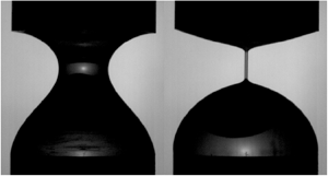
  $L_p$ where the liquid bridge is still stable, as in the left-hand inset image of figure 2(a), but close to the bridge instability threshold. Then, instead of moving the top plate at a constant (lower) velocity, i.e. as in the SRM (Campo-Deano & Clasen Reference Campo-Deano and Clasen2010), we move it by $10\,\mathrm {\mu }{\rm m}$ $L_p$-increment steps, waiting approximately one second between each step (longer than the solution's relaxation time), which is long enough to ensure that polymers are at equilibrium (no pre-stress) before each new step. At a certain step, the bridge becomes unstable (due to the Rayleigh–Plateau instability) and collapses under the action of surface tension, transiently leading to the formation of a nearly cylindrical filament that is the signature of viscoelastic pinch-off, as shown in the right-hand inset image of figure 2(a). We stop moving the top plate once we reach the step at which the bride collapses. The plate separation distance hence remains constant during the capillary thinning of the bridge/filament.
(a) Time evolution of the minimum bridge/filament radius  $h$ in our slow stepwise plate separation protocol for the ${\rm PEO}_{{aq,1}}$ solution for plate diameter $2R_0 = 3.5\,{\rm mm}$ and a sample volume $V^* = V/R_0^3 \approx 2.4$. Inset images correspond to a stable liquid bridge (left) and a thinning filament (right) of the same liquid, with $2R_0 = 7\,{\rm mm}$ and $V^* \approx 2.4$. (b) Last stable bridge radius $h_0$ against the plate radius $R_0$: for $2R_0$ between $2$ and $7\,{\rm mm}$, and for each plate, $V^* \approx 1.3$, $2.4$ and $3.2$ for the ${\rm PEO}_{{aq,1}}$ and ${\rm PEO}_{{visc,1}}$ solutions; and for $2R_0$ between $2$ and $25\,{\rm mm}$, and a single volume ( $V^* \approx 2.4$ for the smallest plates, and $V^*\approx 0.88$ for the largest plates) for the ${\rm PEO}_{{aq,2}}$, ${\rm PEO}_{{visc,2}}$ and HPAM solutions. Inset images correspond to stable liquid bridges ( $h \ge h_0$) for $2R_0 = 2\,{\rm mm}$ (left, ${\rm PEO}_{{aq,1}}$ solution with $V^* \approx 2.4$) and $2R_0 = 20\,{\rm mm}$ (right, HPAM solution with $V^* \approx 1.0$), the right-hand inset being taken from a phone camera because the lens of the set-up camera (used to take the other inset pictures) did not have a large enough field of view.

The process is recorded by a high-magnification objective mounted on a high-speed camera (Phantom TMX 7510), and images are analysed by a Python code. A typical time evolution of the minimum bridge/filament radius is shown in figure 2(a). Throughout the paper, we use the term ‘bridge’ for times  $t< t_1$ before the onset of the elastic regime, and the term ‘filament’ during the elastic regime ( $t \ge t_1$). This radius, measured at the thinnest point along the bridge/filament profile (see left-hand inset image in figure 2a) and labelled ‘ $h_{{min}}$’ by many authors, is simply referred to as $h$ in the rest of the paper. Note that each step can trigger small inertio-capillary oscillations that increase in intensity as the Rayleigh–Plateau instability threshold is approached; see figure 2(a), where oscillations vanish after approximately $0.2$ s for the ${\rm PEO}_{{aq,1}}$ solution. The purpose of this step-by-step plate separation protocol is to identify the last stable liquid bridge configuration and to extract the value of its (minimum) radius $h_0$. Since steps are small, $h_0$ can be considered to be the initial bridge radius at the onset of capillary thinning. Our image resolution is up to 1 pixel per micrometre for the smallest drops, corresponding to the smallest plates, and our time resolution is $15\,000$ images per second to capture the fast bridge collapse from radius $h_0$ to the radius $h_1$ marking the onset of the elastic regime; see figure 2(a).
The liquid bridge becomes unstable at a critical plate separation distance  $L_p = L_p^*$ marking the Rayleigh–Plateau instability threshold. The critical aspect ratio $\varLambda ^* = L_p^*/(2 R_0)$ depends on the liquid volume $V$ and on the Bond number ${Bo} = \rho g R_0^2 / \gamma$, where $g$ is the gravitational acceleration (Slobozhanin & Perales Reference Slobozhanin and Perales1993; Montanero & Ponce-Torres Reference Montanero and Ponce-Torres2020). In our experiments, we vary the plate diameter $2R_0$ between $2$ and $25\,{\rm mm}$, as well as the non-dimensional sample volume
 \begin{equation} V^* = V/R_0^3. \end{equation}
Note that using  $R_0^3$ as a reference volume is an arbitrary choice. Other authors often use the volume ${\rm \pi} R_0^2 L_p^*$ between the plates. As shown in figure 2(b), the last stable bridge radius increases approximately linearly with the plate radius, i.e. $h_0 \propto R_0$ with a prefactor that increases with $V^*$, with no strong dependence on the liquid used since they all have comparable surface tensions. Typically, $h_0/R_0$ ranges between $0.24$ and $0.35$ for $V^* \approx 1.3$ and $3.2$, respectively.
The size difference between the top and bottom end drops, visible in the inset images of figures 2(a,b), stems from Bond numbers  ${Bo} = \rho g R_0^2 / \gamma$ increasing from $0.16$ to $25$ as the plate size increases (Pingulkar, Peixinho & Crumeyrolle Reference Pingulkar, Peixinho and Crumeyrolle2021). The ‘filament’ Bond number ${Bo}_f = \rho g L_f h_1 / \gamma$, however, comparing the typical capillary pressure $\gamma / h_1$ in the filament to the hydrostatic pressure $\rho g L_f$ over the filament length $L_f$, is only up to $0.1$ for the largest plate, indicating that the thinning dynamics is not driven by gravity. The filament length $L_f$, shown in the right-hand inset image of figure 2(a), is discussed in the Appendix.
The aluminium plates are plasma-treated before each measurement to increase their hydrophilicity and hence prevent dewetting of the top plate. However, dewetting could not be avoided for plate diameters  $2R_0 \ge 10\,{\rm mm}$, as shown in the right-hand inset image of figure 2(b), featuring a stable liquid bridge ( $h \ge h_0$) where the top end drop does not fully cover the top plate for $2R_0 = 20\,{\rm mm}$. Perhaps surprisingly, $h_0$ does not saturate at $2R_0 \ge 10\,{\rm mm}$ in spite of this lack of full coverage; see figure 2(b). For such large plates, the top end drop is not necessarily at the centre of the top plate since the two plates are not perfectly parallel. Note that because of the plasma treatment, there is always a thin film covering the top plate.
All experiments are carried out at a high relative humidity ( ${>}80\,\%$) ensured by placing the CaBER set-up in a box with wet paper tissues. We checked that repeating an experiment several times over the course of $10$ min does not lead to any monotonic increase or decrease of the filament thinning rate (defined as $1/3\tau _e$; see § 3) over time, beyond small variations of less than $5\,\%$, suggesting that both evaporation and polymer degradation (which may occur during bridge/filament thinning) are negligible.
2.4. Equations and numerical methods
The numerical simulations discussed in §§ 4 and 5 are performed using the FENE-P model, which aims to describe the stretching and finite extensibility of polymer chains. We consider a cylindrical axisymmetric  $(r,z)$ coordinate system aligned with the vertical axis of the liquid bridge. In the simulations, we integrate the mass and momentum conservation equations of general form
 \begin{gather} \boldsymbol{\nabla} \boldsymbol{\cdot} {\boldsymbol v} = 0, \end{gather}
 \begin{gather} \rho\,\frac{{\rm D}{\boldsymbol v}}{{\rm D}t} ={-}\boldsymbol{\nabla} p+\boldsymbol{\nabla}\boldsymbol{\cdot}\boldsymbol \sigma, \end{gather}
where  $\rho$, ${\boldsymbol v}=v_r({ r,z},t)\,{\boldsymbol e}_r+v_z(r,z,t)\,{\boldsymbol e}_z$ and $p({ r,z},t)$ are the density, velocity and (reduced) pressure fields (accounting for gravity), respectively, and ${\rm D}/{\rm D}t$ is the material derivative. These equations are completed with the constitutive relationships for the stress tensor $\boldsymbol \sigma = \boldsymbol \sigma _s+\boldsymbol \sigma _p$, where
 \begin{equation} \boldsymbol \sigma_s = \eta_s \left(\boldsymbol{\nabla}{\boldsymbol v} + (\boldsymbol{\nabla}{\boldsymbol v} )^\mathrm{T}\right) \end{equation}
is the contribution of the solvent of viscosity  $\eta _s$, and $\boldsymbol \sigma _p$ is the polymer contribution. In the FENE-P model (Snoeijer et al. Reference Snoeijer, Pandey, Herrada and Eggers2020), this contribution is calculated as
 \begin{equation} {\boldsymbol \sigma}_p = \frac{\eta_p}{\tau}\,(f\boldsymbol{\mathsf{A}}-\boldsymbol{\mathsf{I}}), \quad f = \frac{1}{1-\text{tr}(\boldsymbol{\mathsf{A}})/L^2}, \end{equation}
where  $\eta _p$ is the polymer contribution to the zero-shear viscosity $\eta _0 = \eta _s + \eta _p$, $\tau$ represents the relaxation time, and $L^2$ denotes the finite extensibility limit, with $\boldsymbol{\mathsf{I}}$ the identity matrix. The conformation tensor $\boldsymbol{\mathsf{A}}$ is calculated from the nonlinear relaxation law
 \begin{equation} \frac{\mathrm{D} \boldsymbol{\mathsf{A}}}{\mathrm{D} t} - \left[ (\boldsymbol{\nabla}{\boldsymbol v})^\mathrm{T} \boldsymbol{\cdot} \boldsymbol{\mathsf{A}} + \boldsymbol{\mathsf{A}} \boldsymbol{\cdot} \boldsymbol{\nabla}{\boldsymbol v} \right] ={-} \frac{1}{\tau}\,(f \boldsymbol{\mathsf{A}}-\boldsymbol{\mathsf{I}}). \end{equation}
 The free-surface location is defined by the equation  $r=h(z,t)$. The boundary conditions at that surface are
 \begin{gather} \frac{\partial h}{\partial t}+h_z w-u=0, \end{gather}
 \begin{gather} -p+gz-\frac{hh_{zz}-1-h_z^{2}}{h(1+h_z^{2})^{3/2}}+{\boldsymbol n}\boldsymbol{\cdot} {\boldsymbol \sigma}\boldsymbol{\cdot} {\boldsymbol n}=0, \end{gather}
 \begin{gather} {\boldsymbol t}\boldsymbol{\cdot} {\boldsymbol \sigma}\boldsymbol{\cdot} {\boldsymbol n}=0, \end{gather}
where  $h_z \equiv \partial h/\partial z$, $h_{zz} \equiv \partial ^2h/\partial z^2$, $g$ is the gravitational acceleration, ${\boldsymbol n}$ is the unit outward normal vector, and ${\boldsymbol t}$ is the unit vector tangential to the free-surface meridians. Equation (2.9) is the kinematic compatibility condition, while (2.10) and (2.11) express the balance of normal and tangential stresses, respectively. The anchorage condition $h=R_0$ is set at $z=0$ and $z=L_p$, where $L_p$ is the plate separation distance. The no-slip boundary condition is imposed at the solid surfaces in contact with the liquid. The liquid volume $V$ of the initial configuration is prescribed (and conserved), namely,
 \begin{equation} {\rm \pi}\int_{0}^{L_p} h^2\,{\rm d}z=V. \end{equation}
 We start the simulation from a liquid bridge at equilibrium with a plate separation distance  $L_p$ just below (very close to) the critical one. The breakup process is triggered by applying a very small gravitational force perturbation. We refer to the minimum radius of the (stable) liquid bridge just before the perturbation is applied as $h_0$ due to the similarities with the experimental stepwise plate separation protocol described in § 2.3.
A numerical simulation is fully determined by five quantities: the Ohnesorge number, the Deborah number, the non-dimensional sample volume  $V^* = V/R_0^3$, the finite extensibility parameter $L^2$, and the viscosity ratio
 \begin{equation} S = \eta_s / \eta_0. \end{equation}
While equations are non-dimensionalised using  $R_0$ and $(\rho R_0^3 / \gamma )^{1/2}$ as the characteristic length and time scales, in §§ 4 and 5 we refer only to values involving $h_0$ since, as we will show in § 3.1, it is $h_0$ (not $R_0$) that is the most relevant length scale of the problem. In particular, we refer to the Rayleigh and viscous time scales, and Ohnesorge and Deborah numbers defined in (1.3)–(1.6).
Simulations are performed in the absence of gravity where the threshold of the Rayleigh–Plateau instability – and therefore the shape of the initial bridge of minimum radius  $h_0$ from which simulations start – is determined solely by $V^*$. In §§ 4 and 5, instead of referring to $V^*$, we refer to the value of $h_0/R_0$, since in experiments $h_0/R_0$ is set not only by $V^*$ but also by the Bond number. We recall that in experiments, $h_0/R_0$ ranges between $0.24$ and $0.35$ for $V^* \approx 1.3$ and $3.2$, respectively; see figure 2(b).
The model was solved with a variation of the method described in Herrada & Montanero (Reference Herrada and Montanero2016). The physical domain occupied by the liquid is mapped onto a rectangular domain through a coordinate transformation. Each variable, and its spatial and temporal derivatives appearing in the transformed equations, was written as a single symbolic vector. Then we used a symbolic toolbox to calculate the analytical Jacobians of all the equations with respect to the symbolic vector. Using these analytical Jacobians, we generated functions that could be evaluated in the iterations at each point of the discretised numerical domains.
The transformed spatial domain is discretised using  $n_\eta =11$ Chebyshev spectral collocation points in the transformed radial direction $\eta$ of the domain. We used $n_\xi =501$ equally spaced collocation points in the transformed axial direction $\xi$. The axial direction was discretised using second finite differences. Second-order backward finite differences were used to discretise the time domain. We used an automatic variable time step based on the norm of the difference between the solution calculated with a first-order approximation and that obtained from the second-order procedure. The nonlinear system of discretised equations was solved at each time step using the Newton method. The method is fully implicit.
3. Experimental results
In this experimental section, we investigate the roles of the plate radius and sample volume in § 3.1, and of the polymer concentration in § 3.2 on the pinch-off dynamics.
3.1. Influence of the plate radius and sample volume
Image sequences of the pinch-off dynamics are shown in figures 3(a) and 3(b) for the  ${\rm PEO}_{{aq,1}}$ solution ( $500\,{\rm ppm}$ PEO-4M in water) and the ${\rm PEO}_{{visc,1}}$ solution ( $25\,{\rm ppm}$ PEO-4M in a $\sim 260$ more viscous solvent), respectively, illustrating the transition from a bridge shape in the Newtonian regime to a filament shape in the elastic regime. For the ${\rm PEO}_{{aq,1}}$ solution, the filament is initially cylindrical until localised pinching is observed near one of the end drops (see frame 6 in figure 3a), followed by its destabilisation into a succession of beads connected by thin filaments (which are below our spatial resolution), a phenomenon usually referred to as ‘blistering’ instability (Sattler, Wagner & Eggers Reference Sattler, Wagner and Eggers2008; Sattler et al. Reference Sattler, Gier, Eggers and Wagner2012; Eggers Reference Eggers2014; Semakov et al. Reference Semakov, Kulichikhin, Tereshin, Antonov and Malkin2015) (see frames 7 and 8). For the ${\rm PEO}_{{visc,1}}$ solution, local pinching occurs very close to breakup, and no blistering is observed. In this paper, we refer to the minimum bridge/filament radius $h$, which therefore corresponds to the pinched region if localised pinching occurs. On another note, inertio-capillary oscillations of the top and bottom end drops lead to oscillations of the filament length for the ${\rm PEO}_{{aq,1}}$ solution (see frames 3–6 in figure 3a). These oscillations are absent for the ${\rm PEO}_{{visc,1}}$ solution due to viscous damping. Note that oscillations do not lead to significant oscillations of the filament radius, implying that when the length of the filament increases, new filament is being created from the liquid in the end drops.
(a,b) Image sequences of the bridge/filament for the (a)  ${\rm PEO}_{{aq,1}}$ and (b) ${\rm PEO}_{{visc,1}}$ solutions tested with plate diameter $2R_0 = 5\,{\rm mm}$ and sample volume $V^* \approx 2.4$. (c–f) Time evolution of the minimum bridge/filament radius $h$ in (c,e) semi-log and (d, f) lin–lin, for plate diameters $2R_0$ between $2$ and $7\,{\rm mm}$, and fixed $V^* \approx 2.4$, for the (c,d) ${\rm PEO}_{{aq,1}}$ and (e, f) ${\rm PEO}_{{visc,1}}$ solutions, and for their respective solvents (smaller data points), compared with (3.1) and (3.2), where $t_c$ is the solvent breakup time. Times with labels 1–7 and 2–5 in (c,e), respectively, for $2R_0=5\,{\rm mm}$, correspond to the snapshots in (a,b).

Time evolutions of the minimum bridge/filament radius  $h$ are shown in figures 3(c–f) for four plate diameters between $2$ and $7\,{\rm mm}$, and a fixed non-dimensional sample volume $V^* \approx 2.4$ for the ${\rm PEO}_{{aq,1}}$ solution (figures 3c,d) and the ${\rm PEO}_{{visc,1}}$ solution (figures 3e, f) in semi-log (figures 3c,e) and lin–lin (figures 3d, f), the latter focusing on the transition to the elastic regime. The smaller data points correspond to the solvent alone for three of the same plate diameters, and in each case, the same $V^*$ (to within experimental reproducibility). The time reference $t_c$ corresponds to the critical time at which the bridge of solvent alone breaks up. For polymer solutions, since $t_c$ cannot be determined, curves are shifted along the time axis until overlapping their corresponding solvent curves. The good overlap between polymer solutions and their solvent at all times $t< t_1$ (before the transition to the elastic regime) confirms that polymers do not affect the pinch-off dynamics in the (hence rightfully called) Newtonian regime. For the ${\rm PEO}_{{visc,1}}$ solution, where, as is about to be discussed, capillarity is balanced by viscosity in the Newtonian regime, this solution–solvent overlap is consistent with the low polymer contribution to the total shear viscosity ( $\eta _p / \eta _0 = 0.013$). The least good solution–solvent overlaps are explained by experimental differences in $V^*$.
All curves corresponding to Newtonian solvents in figures 3(d, f) overlap close to breakup, indicating a self-similar thinning regime where the initial condition, set by  $R_0$ and $V^*$, is forgotten. Such overlap is also observed for droplets of different volumes for a given plate radius. For the water solvent in figure 3(d), the self-similar regime is well captured by the inertio-capillary thinning law
 \begin{equation} h = A \left( \frac{\gamma}{\rho} \right)^{1/3} (t_c-t)^{2/3}, \end{equation}
with a prefactor  $A = 0.47$ that is consistent with the experimental and numerical results of Deblais et al. (Reference Deblais, Herrada, Hauner, Velikov, Van Roon, Kellay, Eggers and Bonn2018). For the $\sim 260$ times more viscous solvent in figure 3( f), the self-similar regime is well captured by the visco-capillary thinning law (Papageorgiou Reference Papageorgiou1995; McKinley & Tripathi Reference McKinley and Tripathi2000)
 \begin{equation} h = 0.0709\,\frac{\gamma}{\eta_0}\,(t_c-t). \end{equation}
This is consistent with the fact that the Ohnesorge number  ${Oh} = \eta _0/\sqrt {\rho \gamma h_0}$ (see (1.5)) is up to $0.02$ for ${\rm PEO}_{{aq}}$, and up to $0.1$ for HPAM (for the smallest plate diameter where $h_0$ is lowest), i.e. ${Oh} \ll 1$, and ranges between $1.0$ and $2.0$ for the ${\rm PEO}_{{visc,1}}$ solution in the range of plate diameters considered in figure 3. In spite of the moderate Ohnesorge numbers in the latter case, we do not observe a clear transition to the inertio-visco-capillary thinning law $h = 0.0304 (\gamma /\eta _0) (t_c-t)$ (Eggers Reference Eggers1993, Reference Eggers1997; Li & Sprittles Reference Li and Sprittles2016; Verbeke et al. Reference Verbeke, Formenti, Vangosa, Mitrias, Reddy, Anderson and Clasen2020) that describes the behaviour of Newtonian fluids close to breakup; see figure 3(d).
Interestingly, the transition to the elastic regime occurs at approximately the time at which the self-similar Newtonian regime is reached in figures 3(d, f) – slightly after for the  ${\rm PEO}_{{aq,1}}$ solution, and slightly before for the ${\rm PEO}_{{visc,1}}$ solution. However, in both cases, the transition radius $h_1 = h(t_1)$ increases with the plate diameter $2R_0$, which indicates that polymers already started to deform significantly before the self-similar regime. Indeed, if polymers started to deform only within the self-similar regime where the thinning dynamics no longer depends on $R_0$ or $V^*$, then the amount of polymer deformation would be independent of the initial condition, leading to a transition radius $h_1$ that would not depend on $R_0$ or $V^*$, as we discuss further in § 4.3.
After the filament formation, the thinning rate  $\vert \dot {h}/h \vert$ is initially fairly constant, indicating an exponential decay, and increases close to breakup in a so-called ‘terminal regime’ where authors argue that polymer chains approach full extension and a Newtonian-like high-viscosity dynamics is recovered (Anna & McKinley Reference Anna and McKinley2001; Stelter et al. Reference Stelter, Brenn, Yarin, Singh and Durst2002; Campo-Deano & Clasen Reference Campo-Deano and Clasen2010; Dinic & Sharma Reference Dinic and Sharma2019). The (constant) filament thinning rate measured during the exponential part of the elastic regime is found to decrease with increasing plate diameter; see figures 3(c,e). This is inconsistent with the Oldroyd-B model, which predicts $\vert \dot {h}/h \vert = 1/3\tau$ (see (1.1)), where $\tau$ is the (longest) relaxation time of the polymer solution, which is a fluid property, independent of the size of the system. As we show in our previous paper (Gaillard et al. Reference Gaillard, Herrada, Deblais, Eggers and Bonn2024), this surprising dependence on the system size is also observed for the classical step-strain plate separation protocol of a commercial CaBER rheometer as well as for DoS and dripping (Rajesh et al. Reference Rajesh, Thiévenaz and Sauret2022) experiments. We show that this is not caused by artefacts such as solvent evaporation or polymer degradation, suggesting that the liquid does not change when being tested with different plate diameters. To discuss this geometry-dependent filament thinning rate, we define an apparent (or effective) relaxation time $\tau _e$ such that $\vert \dot {h}/h \vert = 1/3\tau _e$ during the exponential part of the elastic regime.
The apparent relaxation time  $\tau _e$ and the transition radius $h_1$ are plotted against $h_0$ in figure 4 for different polymer solutions, plate diameters $2R_0$ and non-dimensional sample volumes $V^*$. The fact that data corresponding to different values of $R_0$ and $V^*$ collapse on a single curve for both the ${\rm PEO}_{{aq,1}}$ and ${\rm PEO}_{{visc,1}}$ solutions suggests that $h_0$, which is an increasing function of both $R_0$ and $V^*$ (see figure 2b), is the only relevant geometrical parameter of the problem. This is the reason why we chose $h_0$ at the relevant length scale for non-dimensional numbers such as the Ohnesorge and Deborah numbers in (1.5) and (1.6). This is in agreement with the idea that the thinning dynamics is influenced only by extensional flow in the bridge/filament, while the top and bottom end droplets act as passive liquid reservoirs.
(a) Effective extensional relaxation time  $\tau _e$ and (b) transition radius $h_1$ against the last stable bridge radius $h_0$ for different plate radii $R_0$ and sample volumes $V^*$ for all polymer solutions. For the ${\rm PEO}_{{aq,1}}$ and ${\rm PEO}_{{visc,1}}$ solutions, three points of the same colour correspond to the same $R_0$ and three different $V^* \approx 1.3$, $2.4$ and $3.2$.

We find that  $\tau _e$ seems to saturate towards a maximum value $\tau _m$ at large $h_0$; see figure 4(a). The estimated values of $\tau _m$ are reported in table 2 for the ${\rm PEO}_{{aq,2}}$, ${\rm PEO}_{{visc,2}}$ and HPAM solutions for which plate diameters up to $25\,{\rm mm}$ were used, well beyond typical CaBER plate sizes, which was needed to observe the saturation of $\tau _e$. In our previous paper (Gaillard et al. Reference Gaillard, Herrada, Deblais, Eggers and Bonn2024), we explored the possibility that $\tau _m$ could be the ‘real’ relaxation time of the solution, invoking finite extensibility effects described by the FENE-P model to explain thinning rates larger than $1/3\tau _m$ for low $h_0$. We concluded that this was a possible explanation only for the ${\rm PEO}_{{visc,2}}$ solution, not for the ${\rm PEO}_{{aq,2}}$ and HPAM solutions, suggesting that the FENE-P model misses some important features of polymer dynamics in extensional flows.
The first transition radius  $h_1$ increases approximately linearly with $h_0$ for all liquids; see figure 4(b). This is in contradiction with the scaling $h_1 \propto h_0^{4/3}$ expected from the Oldroyd-B model when assuming that polymer relaxation is negligible during the time needed for the bridge to thin from $h_0$ to $h_1$; see (1.2). Since $h_0 \propto R_0$ for a fixed $V^*$ (see figure 2b), this implies that $h_1 \propto R_0$, different from the scaling $h_1 \propto R_{n}^{0.66}$ observed experimentally by Rajesh et al. (Reference Rajesh, Thiévenaz and Sauret2022) in the analogous problem of a drop falling from a nozzle of radius $R_n$. This is surprising since $R_n$ should play the same role as the plate radius $R_0$ in CaBER.
Note that the  ${\rm PEO}_{{aq,2}}$ and ${\rm PEO}_{{visc,2}}$ solutions are slightly more elastic than the ${\rm PEO}_{{aq,1}}$ and ${\rm PEO}_{{visc,1}}$ solutions, since they exhibit larger apparent relaxation times; see figure 4(a). However, these differences are barely visible in figure 4(b) since the values of $h_1$ are almost the same, suggesting that the dependence of $h_1$ on $\tau _e$ is relatively weak, as we now confirm by varying the polymer concentration.
3.2. Influence of the polymer concentration
Figure 5 shows the time evolution of the minimum bridge/filament radius for the aqueous PEO solutions of table 1 of various PEO concentrations, water solvent included, that were tested for a fixed plate diameter  $2R_0 = 3.5\,{\rm mm}$ and sample volume $V^* \approx 2.4$, in semi-log (figure 5a) and in lin–lin focusing on the transition to the elastic regime (figure 5b). As in figure 3, the time $t_c$ at which the solvent breaks is chosen as the time reference, and curves corresponding to polymer solutions are shifted along the time axis to maximise the overlap with the solvent for $t< t_1$. This overlap is very good up to $2500\,{\rm ppm}$ (dilute and unentangled semi-dilute solution), small deviations being attributable to slightly different sample volumes. For $10\,000\,{\rm ppm}$ (entangled semi-dilute solution), however, the bridge dynamics prior to the exponential regime is radically different from the pure solvent case, indicating that elasticity is not negligible even before the exponential regime is reached.
Time evolution of the minimum bridge/filament radius  $h$ in (a) lin–log and (b) lin–lin focusing on the transition, for PEO-4M solutions of different concentrations in water, for a fixed plate diameter $2R_0 = 3.5\,{\rm mm}$ and sample volume $V^* \approx 2.4$. The time $t_c$ is the time at which the bridge would break up for the solvent alone, here water.

The apparent relaxation time  $\tau _e$ and the transition radius $h_1$ are plotted in figure 6 as functions of the polymer concentration $c$ for the aqueous PEO solutions of table 1. Since these solutions were tested for a fixed plate diameter $2R_0 = 3.5\,{\rm mm}$ and sample volume $V^* \approx 2.4$, the initial bridge radius $h_0 \approx 460\,\mathrm {\mu }{\rm m}$, also plotted in figure 6(b), is the same for each solution. For the $500\,{\rm ppm}$ solution, labelled ${\rm PEO}_{{aq,1}}$ – which was tested for four plate diameters from $2$ to $7\,{\rm mm}$, and in each case with three different volumes – the corresponding values of $\tau _e$, $h_0$ and $h_1$ are also included in figure 6 to illustrate how data for a given concentration can shift as $h_0$ is varied. Although the plate diameters used for the ${\rm PEO}_{{aq,1}}$ solution were not large enough to estimate the high- $h_0$ limit value of $\tau _e$, $\tau _m$, the value estimated for the slightly more elastic ${\rm PEO}_{{aq,2}}$ solution (see figure 4(a) and table 2), is shown in figure 6(a) for $c=500\,{\rm ppm}$.
(a) Relaxation times and (b) transition radius  $h_1$ and last stable bridge radius $h_0$ against polymer concentration for PEO-4M solutions of different concentrations in water. The data of (b) and the effective CaBER relaxation time $\tau _e$ in (a) correspond to a fixed plate diameter $2R_0 = 3.5\,{\rm mm}$ and sample volume $V^* \approx 2.4$, except for the 500 ppm solution, where data corresponding to different $2R_0$ (between $2$ and $7\,{\rm mm}$) and $V^*$ are shown. In (a), we also plot the relaxation time $1/\dot {\gamma }_c$ and $\varPsi _1/ 2 \eta _p$ inferred from shear rheology, as well as the Zimm relaxation time $\tau _Z$. We also show the maximum CaBER relaxation time $\tau _m$ (high- $h_0$ limit of $\tau _e$) measured for the ( $500\,{\rm ppm}$) ${\rm PEO}_{{aq,2}}$ solution (which is slightly more elastic than the ${\rm PEO}_{{aq,1}}$ solution from which the other $500\,{\rm ppm}$ data points are taken; see figure 4a). Error bars are shown in (a) but are smaller than markers for $\tau _e$.

We find a weak dependence  $h_1 \propto c^{0.16}$ for dilute and semi-dilute solutions (see figure 6b), consistent with Rajesh et al. (Reference Rajesh, Thiévenaz and Sauret2022), who found $h_1 \propto c^{0.15}$ in the analogous problem of a drop falling from a nozzle. We find a power law $\tau _e \propto c^{0.85}$ for the apparent relaxation time in figure 6(a), consistent with the wide range of exponents, typically between $0.6$ and $1$, reported by other authors in CaBER (Bazilevsky et al. Reference Bazilevsky, Entov, Lerner and Rozhkov1997; Clasen et al. Reference Clasen, Plog, Kulicke, Owens, Macosko, Scriven, Verani and McKinley2006b; Zell et al. Reference Zell, Gier, Rafai and Wagner2010) and pendant drop experiments (Tirtaatmadja et al. Reference Tirtaatmadja, McKinley and Cooper-White2006; Rajesh et al. Reference Rajesh, Thiévenaz and Sauret2022). Note that this exponent is expected to be a function of the solvent quality (Clasen et al. Reference Clasen, Plog, Kulicke, Owens, Macosko, Scriven, Verani and McKinley2006b) and that its potential dependence on $h_0$ is not investigated in the present work. From these scalings, we deduce a weak dependence of $h_1 \propto \tau _e^{0.19}$ on the apparent relaxation time.
The apparent CaBER relaxation time  $\tau _e$ in figure 6(a) is compared to values estimated from shear rheology, i.e. $1/\dot {\gamma }_c$, which is estimated from shear viscosity curves featuring shear thinning, which excludes low concentrations, and $\varPsi _1 / 2 \eta _p$, which is estimated from the first normal stress difference for the only two measurable solutions exhibiting a quadratic scaling $N_1 \propto \dot {\gamma }^2$. We observe that $1/\dot {\gamma }_c$ follows a power law with an exponent close to the one found for $\tau _e$. Additionally, we find that $\tau _e$ is larger than $\varPsi _1 / 2 \eta _p$ in figure 6(a) for this specific plate radius, and would hence be even larger in the high- $h_0$ limit $\tau _m$. Hence even for dilute solutions exhibiting weak shear thinning and quadratic normal stresses, for which the Oldroyd-B model could describe the shear rheology, there is no quantitative agreement between the relaxation time measured from normal stresses and that from filament thinning rheometry. This impossibility to quantitatively describe both shear and elongation properties with the Oldroyd-B model has also been reported by Zell et al. (Reference Zell, Gier, Rafai and Wagner2010), who dedicated a paper specifically to the link between $\tau _e$ and $\varPsi _1$. In a recent perspective paper, Boyko & Stone (Reference Boyko and Stone2024) suggest that the reason why elastic dumbbell models such as Oldroyd-B and FENE-P cannot quantitatively predict both shear and elongation properties of polymer solutions is because these models assume that, as in elongation flows, polymer chains approach full extension in strong shear flows ( $\tau \dot {\gamma } \gg 1$), while experimentally, chains have been observed to extend only partially in strong shear flows due to their tumbling motion (Smith, Babcock & Chu Reference Smith, Babcock and Chu1999). The authors hence suggest that flows with both shear and elongational components should be described using more complex models such as the FENE-PTML model (Phan-Thien, Manero & Leal Reference Phan-Thien, Manero and Leal1984), which captures this partial extension under shear. In this paper, we consider only filament thinning elongational flows for which Oldroyd-B and FENE-P are suitable model candidates.
As shown in figure 6(a), the apparent CaBER relaxation time  $\tau _e$ increases in the dilute regime $c< c^*$. Moreover, for the most dilute solutions, $\tau_e$ is less than the Zimm relaxation time calculated using (Clasen et al. Reference Clasen, Plog, Kulicke, Owens, Macosko, Scriven, Verani and McKinley2006b)
 \begin{equation} \tau_Z = \frac{1}{\zeta(3 \nu)}\,\frac{[\eta] M_w \eta_s}{N_a k_B T}, \end{equation}
where  $N_a$ is the Avogadro number, $k_B$ is the Boltzmann constant, $T$ is the temperature, $\zeta$ is the Riemann zeta function, and $\nu$ is the solvent quality exponent. We used $\nu = 0.55$ between theta and good solvent to find $\tau _Z = 2.0$ ms. Similar results were reported by Clasen et al. (Reference Clasen, Plog, Kulicke, Owens, Macosko, Scriven, Verani and McKinley2006b), who argue that the increase of $\tau _e$ in the dilute regime is caused by a self-concentration effect where chains start to interact while unravelling well beyond their equilibrium size in strong extensional flows. This was later rationalised by Prabhakar et al. (Reference Prabhakar, Gadkari, Gopesh and Shaw2016), who argue that the Zimm relaxation time is relevant only close to equilibrium, even for dilute solutions, and is not expected to accurately describe the relaxation behaviour of polymer chains in strong extensional flows such as in filament thinning. Clasen et al. (Reference Clasen, Plog, Kulicke, Owens, Macosko, Scriven, Verani and McKinley2006b) and Prabhakar et al. (Reference Prabhakar, Gadkari, Gopesh and Shaw2016), who considered only cases where inertia was negligible in the Newtonian regime, also show that values $\tau _e < \tau _Z$ arise at low polymer concentration where elasticity is too weak to fully overcome the solvent viscosity in the elastic regime. This effect should, however, be negligible for the aqueous PEO solutions of figure 6(a) since it is inertia (and not the solvent viscosity) that dominates in the Newtonian regime (see figure 5b). We show in § 5 that values $\tau _e < \tau _Z$ at low concentrations are consistent with polymer chains approaching their finite extensibility limit at the onset of the elastic regime (as anticipated by Campo-Deano & Clasen Reference Campo-Deano and Clasen2010), a case where (1.1) is no longer valid, and filament thinning rates $\vert \dot {h}/h \vert > 1/3\tau$ are to be expected, as we show in our previous paper (Gaillard et al. Reference Gaillard, Herrada, Deblais, Eggers and Bonn2024).
4. Oldroyd-B prediction for  $h_1$
$h_1$

In order to rationalise the experimental findings of § 3, we need to expand the polymer-relaxation-free theory leading to (1.2) for  $h_1$ to cases where polymer relaxation is not negligible in the Newtonian regime. A generalised theoretical expression for $h_1$ based on the Oldroyd-B model is first derived in § 4.1. This expression is then tested against experimental results in § 4.2, before we use numerical simulations in § 4.3 to validate the theory and further explore the role of non-negligible polymer relaxation on $h_1$.
4.1. Theory
The filament radius  $h_1=h(t_1)$ marks the transition between the Newtonian regime ( $t< t_1$), where the driving capillary force is balanced by inertia and/or viscosity, and the elastic regime ( $t>t_1$), where capillarity is balanced by elastic stresses arising from the stretching of polymer chains. If inertia is negligible, then slender filament theory predicts that the total (unknown) tensile force $T$ is constant along the liquid column (bridge or filament) (Eggers Reference Eggers1997; Clasen et al. Reference Clasen, Eggers, Fontelos, Li and McKinley2006a), which, neglecting gravity and axial curvature effects, results in the zero-dimensional force balance equation (Clasen et al. Reference Clasen, Plog, Kulicke, Owens, Macosko, Scriven, Verani and McKinley2006b)
 \begin{equation} (2X-1)\,\frac{\gamma}{h} = 3 \eta_s \dot{\epsilon} + \sigma_{p,zz} - \sigma_{p,rr}, \end{equation}
for a column of radius  $h$. The driving capillary pressure $\gamma /h$ is balanced by the normal stress difference $\sigma _{zz} - \sigma _{rr}$, which is the sum of the solvent viscous stress $3 \eta _s \dot {\epsilon }$ and the polymeric stress $\sigma _{p,zz} - \sigma _{p,rr}$, where $\dot {\epsilon } = -2 \dot {h}/h$ is the extension rate, the dot standing for $\mathrm {d}/\mathrm {d}t$, and $z$ is the direction of the flow. The ratio $X = T / 2 {\rm \pi}\gamma h$ may vary over time, approaching $X=0.7127$ for a Newtonian fluid (McKinley & Tripathi Reference McKinley and Tripathi2000), hence recovering (3.2) close to breakup, and approaching $X=3/2$ in the elastic regime for an Oldroyd-B fluid (Eggers, Herrada & Snoeijer Reference Eggers, Herrada and Snoeijer2020) (and not $X=1$ as originally proposed in Entov & Hinch Reference Entov and Hinch1997). When inertia is not negligible, Tirtaatmadja et al. (Reference Tirtaatmadja, McKinley and Cooper-White2006) suggested adding a term of the form $\tfrac {1}{2} \rho \dot {h}^2$ to (4.1), from which the inertio-capillary scaling of (3.1) is recovered. In the elastic regime ( $t>t_1$), assuming that inertia and/or solvent viscosity has become negligible, and assuming that the axial stress dominates the radial stress, i.e. $\vert \sigma _{p,rr} \vert \ll \vert \sigma _{p,zz} \vert$, the force balance equation reduces to
 \begin{equation} (2X-1)\,\frac{\gamma}{h} = \sigma_{p,zz}. \end{equation}
 The elastic regime starts when the polymeric axial stress  $\sigma _{p,zz}$ – which increases over time in the Newtonian regime as polymer chains are progressively stretched by the extensional flow in the thinning bridge – becomes of the order of the capillary pressure, say, when it is equal to fraction $p$ of the capillary pressure (Campo-Deano & Clasen (Reference Campo-Deano and Clasen2010) chose $p=1/2$). We hence get that $p \gamma /h_1 = \sigma _{p,zz}(t=t_1)$ where, for simplicity, the prefactor $2X-1$ of order unity has been included in the prefactor $p$. To estimate $h_1$, we hence need to choose a constitutive equation to express the polymeric stress. Since our main goal is to understand the effect of polymer relaxation during the Newtonian regime on $h_1$, which, when negligible, leads to (1.2) for a single-mode Oldroyd-B fluid, we choose to use this model for simplicity. Indeed, although we know that the Oldroyd-B model is unable to capture the system-size dependence of the apparent relaxation time $\tau _e$ discussed in our previous paper (Gaillard et al. Reference Gaillard, Herrada, Deblais, Eggers and Bonn2024) (see also figures 3 and 4a), it is not yet clear whether or not it is able capture $h_1$. Finite extensibility effects on $h_1$ will be discussed in § 5 using the FENE-P model.
For an Oldroyd-B fluid with elastic modulus  $G$, we have $\sigma _{p,zz} = G ({\mathsf{A}}_{zz} - 1)$, where ${\mathsf{A}}_{zz}$ is the normal part of the conformation tensor $\boldsymbol{\mathsf{A}}$ that follows (see (2.8) and Wagner, Bourouiba & McKinley Reference Wagner, Bourouiba and McKinley2015)
 \begin{equation} \skew6\dot{{\mathsf{A}}}_{zz} - 2 \dot{\epsilon} {\mathsf{A}}_{zz} ={-} \frac{{\mathsf{A}}_{zz}-1}{\tau}, \end{equation}
where  $\tau$ is the relaxation time. Since we are interested in the location of highest polymer extensions along the bridge, we use the expression of the extension rate $\dot {\epsilon } = -2 \dot {h}/h$ at the thinnest point to obtain
 \begin{equation} \skew6\dot{{\mathsf{A}}}_{zz} + \frac{4 \dot{h}}{h}\,{\mathsf{A}}_{zz} ={-} \frac{{\mathsf{A}}_{zz}-1}{\tau}. \end{equation}
Some (as yet unknown) time after the onset of capillary thinning of the liquid bridge, polymer chains will have stretched well beyond their equilibrium size, i.e.  ${\mathsf{A}}_{zz} \gg 1$, so that the right-hand side of (4.4) reduces to $-{\mathsf{A}}_{zz}/\tau$, at which point (4.4) can be integrated into
 \begin{equation} {\mathsf{A}}_{zz} h^4 \propto {\rm e}^{{-}t/\tau}, \end{equation}
with an (as yet unknown) constant prefactor. Polymer chains are expected to remain close to their equilibrium coiled size ( ${\mathsf{A}}_{zz}$ close to $1$) until the extension rate in the thinning bridge approaches the coil–stretch transition value $1/2\tau$ predicted by the Oldroyd-B model. Beyond this point, following Clasen et al. (Reference Clasen, Bico, Entov and McKinley2009) and Campo-Deano & Clasen (Reference Campo-Deano and Clasen2010), we assume that polymer chains unravel with negligible relaxation, i.e. that the right-hand side of (4.4) becomes negligible so that ${\mathsf{A}}_{zz} h^4$ becomes constant. More precisely,
 \begin{equation} {\mathsf{A}}_{zz} h^4 = H^4, \end{equation}
where  $H$ is the (as yet unknown) bridge radius at which relaxation becomes negligible, which should correspond to the coil–stretch transition point at which ${\mathsf{A}}_{zz}$ starts to become significantly larger than $1$. In particular, at the transition to the elastic regime at time $t=t_1$,
 \begin{equation} A_1 = (H/h_1)^4, \end{equation}
where  $A_1 = {\mathsf{A}}_{zz}(t_1)$ quantifies the amount of polymer stretching at the onset of the elastic regime. Since $p \gamma /h_1 = \sigma _{p,zz}(t_1) = G A_1$, we finally get that
 \begin{equation} h_1 = \left( \frac{G H^4}{p \gamma} \right)^{1/3}, \end{equation}
which is different from (1.2). Indeed, while it is assumed that  $H=h_0$ in the polymer-relaxation-free theory leading to (1.2), this is actually true only in the limit where polymer relaxation is negligible throughout the whole Newtonian regime so that ${\mathsf{A}}_{zz} h^4$ is constant and equal to $h_0^4$ since ${\mathsf{A}}_{zz} = 1$ at the onset of capillary thinning, assuming no pre-stress. In other words, in the limit where $H=h_0$, the coil–stretch transition starts at the onset of capillary thinning, which is expected to be true only if the relaxation time $\tau$ is much larger than the time taken by the liquid bridge to thin from $h_0$ to $h_1$. For completeness, in the elastic regime ( $t \ge t_1$), combining (4.5) and (4.2) with $p \gamma /h_1 = G A_1$ leads to the exponential scalings $h = h_1 \exp {(-(t-t_1)/3\tau )}$ in (1.1) and ${\mathsf{A}}_{zz} = A_1 \exp {((t-t_1)/3\tau )}$.
4.2. Experiments
We can now test the generalised expression (4.8) for  $h_1$ against the experimental results of § 3. In order to do so, we first need to compute $H$ from the time-evolution of ${\mathsf{A}}_{zz}$. Note that we do not experimentally measure the extension of polymer chains, unlike Ingremeau & Kellay (Reference Ingremeau and Kellay2013), who confirmed the transition from a coiled to a stretched state in viscoelastic pinch-off using fluorescently labelled DNA. Rather, since our goal is to test a specific constitutive equation, here Oldroyd-B, we calculate its prediction for ${\mathsf{A}}_{zz}(t)$ using (4.4), where the extension rate $\dot {\epsilon } = -2 \dot {h}/h$ is taken from experimental values of $h(t)$. In other words, we calculate the prediction of the model for the experimental history of extension rates in the bridge/filament. In particular, we do not assume large polymer extension ( ${\mathsf{A}}_{zz} \not \gg 1$) since the point at which ${\mathsf{A}}_{zz}$ starts to become significantly larger than $1$ is precisely what sets $H$. Equation (4.4) can in fact be integrated, as shown by Bazilevsky, Entov & Rozhkov (Reference Bazilevsky, Entov and Rozhkov2001), introducing a function $y(t)$ such that ${\mathsf{A}}_{zz} = y \exp {(-t/\tau )} / h^4$, which leads to $\dot {y} = h^4 \exp {(t/\tau )} / \tau$, yielding
 \begin{equation} {\mathsf{A}}_{zz} = \frac{{\rm e}^{{-}t/\tau}}{h^4} \left( h_0^4 \, {\rm e}^{t_0/\tau} + \frac{1}{\tau} \int_{t_0}^t h^4(t')\, {\rm e}^{t'/\tau} \,\mathrm{d} t' \right), \end{equation}
where the initial time  $t_0$ corresponds to the onset of capillary thinning, i.e. $h(t_0) = h_0$ and ${\mathsf{A}}_{zz}(t_0)=1$ (no pre-stress). Since the $h(t)$ history is set by the experimental data, the only adjustable parameter of (4.9) is the relaxation time $\tau$. In the following, we use either the apparent ( $\tau _e$) or the maximum ( $\tau _m$) relaxation time measured experimentally (see figure 4a) to calculate ${\mathsf{A}}_{zz}$ since we still do not know which is the ‘true’ one, if any.
Values of  ${\mathsf{A}}_{zz}(t)$ computed from (4.9) using the experimental values of $h(t)$ with relaxation time $\tau = \tau _m$ are shown in figure 7(a) for the ${\rm PEO}_{{aq,2}}$ solution, and in figure 7(b) for the ${\rm PEO}_{{visc,2}}$ solution, for plate diameters $2R_0$ between $2$ and $20\,{\rm mm}$. The experimental values of $h(t)$ are shown on the left-hand $y$-axis, and the time reference $t_1$ corresponds to the onset of the elastic regime. We find that the amount of polymer extension $A_1 = {\mathsf{A}}_{zz}(t_1)$ at the onset of the elastic regime is fairly independent of the initial condition for the ${\rm PEO}_{{aq,2}}$, while for the ${\rm PEO}_{{visc,2}}$ solution, $A_1$ decreases as $h_0(R_0,V^*)$ increases, as mentioned in our previous paper (Gaillard et al. Reference Gaillard, Herrada, Deblais, Eggers and Bonn2024), and as we are about to discuss here in more depth. In any case, we find that ${\mathsf{A}}_{zz}$ always increases as $1/h^4$ in the Newtonian regime close enough to the transition to the elastic regime. More specifically, values of ${\mathsf{A}}_{zz}$ are well captured by $(H/h)^4$ using $H$ as a fitting parameter for each data set (close to $t_1$), from which $H$ is estimated; see figure 7.
Time evolution of the experimental minimum bridge/filament radius  $h$ and of ${\mathsf{A}}_{zz}$, calculated from the Oldroyd-B prediction (4.9) using the experimental values of $h(t)$ with the choice of relaxation time $\tau = \tau _{m}$ (see figure 4a), for plate diameters $2R_0 = 2$, $5$,
$5$,  $10$ and $25\,{\rm mm}$ for the (a) ${\rm PEO}_{{aq,2}}$ and (b) ${\rm PEO}_{{visc,2}}$ solutions. Time $t_1$ marks the onset of the elastic regime, with $h_1 = h(t_1)$ and $A_1 = {\mathsf{A}}_{zz}(t_1)$. Values of ${\mathsf{A}}_{zz}$ in the Newtonian regime ( $t< t_1$) are compared to $(H/h)^4$ (see (4.6)), where $H$ is used as a fitting parameter to optimise the agreement close to $t_1$.

Values of  $H$ calculated using $\tau = \tau _m$, named $H(\tau _m)$, are plotted against $h_0$ in figure 8(a) for the ${\rm PEO}_{{aq,2}}$, ${\rm PEO}_{{visc,2}}$ and HPAM solutions, which are the only solutions for which sufficiently large plate diameters were used to estimate the maximum relaxation time $\tau _m$ (the high- $h_0$ limit of $\tau _e$; see figure 4a). For the ${\rm PEO}_{{aq,2}}$ and HPAM solutions, we find that $H$ is essentially equal to $h_0$ at low $h_0$, and that $H/h_0$ decreases as $h_0$ increases, down to $0.73$ for the largest plate diameter. In contrast, for the ${\rm PEO}_{{visc,2}}$ solution, the ratio $H/h_0$ takes significantly smaller values, decreasing from $0.56$ to $0.40$ as $h_0$ increases. This is why the $(H/h)^4$ fit for ${\mathsf{A}}_{zz}$ is fairly good throughout the whole Newtonian regime for the ${\rm PEO}_{{aq,2}}$ solution in figure 7(a), while it is valid only within a small time window close to the transition to the elastic regime for the ${\rm PEO}_{{visc,2}}$ solution in figure 7(b). Indeed, if $H=h_0$, then the $(H/h)^4$ fit for ${\mathsf{A}}_{zz}$ is even valid at the onset of capillary thinning where $h=h_0$ and ${\mathsf{A}}_{zz} = 1$.
Values of  $H$ estimated from the time evolution of ${\mathsf{A}}_{zz}$ (calculated using Oldroyd-B; see figure 7) using (a) the maximum relaxation time $\tau =\tau _m$ or (b) the effective relaxation time $\tau =\tau _e$, for different polymer solutions and initial bridge radii $h_0(R_0,V^*)$, plotted against $h_0$. The line $H=h_0$ is shown in both plots.

Figure 8(a) hence suggests that although all three solutions have comparable relaxation times (see figure 4a), the thinning dynamics in the Newtonian regime is such that polymer chains stretch almost without relaxing in the Newtonian regime for the low solvent viscosity solutions ( ${\rm PEO}_{{aq,2}}$ and HPAM), while relaxation is not negligible for the high solvent viscosity ( ${\rm PEO}_{{visc,2}}$) solution. This is because the Newtonian thinning dynamics is slower for the most viscous solution; see e.g. figure 7, where, for $2R_0 = 2\,{\rm mm}$, the bridge takes only approximately $6$ ms to thin from $h_0$ to $h_1$ for the ${\rm PEO}_{{aq,2}}$ solution, much less than $\tau _m$ (chains do not have enough time to relax), while it takes approximately $900$ ms for the ${\rm PEO}_{{visc,2}}$, much more than $\tau _m$ (not visible in figure 7(b), where we focus on times close to $t_1$). The fact that $H/h_0$ increases as $h_0$ increases can therefore be interpreted by a longer time to thin from $h_0$ to $h_1$ as $h_0$ increases, consistent with the fact that the Rayleigh and viscous time scales $\tau _R = (\rho h_0^3 / \gamma )^{1/2}$ and $\tau _{{visc}} = \eta _0 h_0 / \gamma$ both increase with $h_0$.
The dependence of  $H$ on $h_0$ and on the solvent viscosity explains why, in figure 7 and in our previous paper (Gaillard et al. Reference Gaillard, Herrada, Deblais, Eggers and Bonn2024), $A_1$ is independent of $h_0$ for low solvent viscosity solutions ( ${\rm PEO}_{{aq,2}}$ and HPAM), while $A_1$ decreases as $h_0$ increases for the high solvent viscosity solution ( ${\rm PEO}_{{visc,2}}$). For the former, where $H$ is close to $h_0$ (negligible polymer relaxation in the Newtonian regime), $A_1 = (H/h_1)^4$ (see (4.7)) is close to $(h_0/h_1)^4$, which is fairly constant since $h_1 \propto h_0$ according to figure 4(b). For the latter, however, where $H \propto h_0^{0.74}$ in our range of $h_0$ according to figure 8(a), we get $A_1 = (H/h_1)^4 \propto h_0^{-1.04}$.
In figure 8(b), we plot the values of  $H$, named $H(\tau _e)$, calculated using the apparent relaxation time $\tau = \tau _e$ when computing ${\mathsf{A}}_{zz}$ from (4.9) (instead of its large- $h_0$ limit $\tau _m$ in figure 8a). All polymer solutions are now featured since $\tau _e$ is measured for any experiment from an exponential fit of $h(t)$ in the exponential part of the elastic regime (see figure 3), i.e. the ${\rm PEO}_{{aq,2}}$, ${\rm PEO}_{{visc,2}}$ and HPAM solutions, as in figure 8(a), but also the ${\rm PEO}_{{aq,1}}$ and ${\rm PEO}_{{visc,1}}$ solutions, where three different non-dimensional sample volumes $V^*$ were tested for each of the four smallest plate diameters, as well as the PEO solutions in water with various polymer concentrations (table 1), which were tested for a single $(R_0,V^*)$ set corresponding to $h_0 \approx 460\,\mathrm {\mu }{\rm m}$. The data corresponding to the PEO solutions with different polymer concentrations $c$ show how, for a given flow history in the Newtonian regime (same $h(t)$ curves for $t< t_1$ for all concentrations; see figure 5), $H$ increases with $c$ via the increase in the relaxation time (here $\tau = \tau _e$), reaching the upper limit value $h_0$ at large $\tau$. This is because for large $\tau$ values, polymer relaxation is negligible throughout the whole Newtonian regime, while for low $\tau$ values, ${\mathsf{A}}_{zz}$ remains equal to $1$ for most of the Newtonian regime, increasing only when $\dot {\epsilon }$ is finally of the order of $1/2\tau$ close to the transition to the elastic regime.
Now that we know the value of  $H$, we can test the validity of (4.8) for the filament radius $h_1$ at the onset of the elastic regime. The value of the elastic modulus, $G = \eta _p/\tau$ in the Oldroyd-B model, is, however, not uniquely defined, since while $\eta _p = \eta _0 - \eta _s$ can be calculated unambiguously from the shear rheology, the relaxation time $\tau$ could be either the apparent one $\tau _e$ or the maximum one $\tau _m$, since we do not know yet which one is the ‘true’ one, if any. We hence need to test for both. To this end, we define
 \begin{equation} G_H = \gamma h_1^3 / H^4, \end{equation}
where  $h_1$ is the value measured experimentally, which should be $G_H = G/p$ according to (4.8).
In figure 9(a),  $G_H$ is plotted against $G$ for the choice of relaxation time $\tau = \tau _m$ for the ${\rm PEO}_{{aq,2}}$, ${\rm PEO}_{{visc,2}}$ and HPAM solutions, which are the only solutions for which sufficiently large plate diameters were used to estimate $\tau _m$. More precisely, values of $G_H(\tau _m)$ calculated from $H(\tau _m)$ are plotted against $G(\tau _m) = \eta _p / \tau _m$, which takes a unique value for each solution since the relaxation time is unique. We find that values of $G_H(\tau _m)$ are, however, not unique for the ${\rm PEO}_{{aq,2}}$ and HPAM solutions, and monotonically decrease as $h_0$ increases. For the ${\rm PEO}_{{visc,2}}$ solution, however, values of $G_H$ vary between $0.11$ and $0.23$ without clear monotonic trend as $h_0$ increases. This is because, since $h_1 \propto h_0$ and $H \propto h_0^{k_H}$ in the range of $h_0$ values investigated, with $k_H \le 1$ (see figures 4b and 8a), $G_H \propto h_1^3 / H^4 \propto h_0^{3-4k_H}$, which means that $G_H$ is expected to be independent of $h_0$ only for $k_H = 0.75$, very close to the value $0.74$ found for the ${\rm PEO}_{{visc,2}}$ solution in figure 8(a). This suggests that the prediction of (4.8) for the choice $\tau = \tau _m$ is potentially valid for only one of our three solutions, the most dilute and viscous one.
Values of  $G_H$ defined in (4.10) against the elastic modulus $G = \eta _p/\tau$, where $H$ and $G$ are calculated from (a) the maximum relaxation time $\tau = \tau _m$ or (b) the effective relaxation time $\tau = \tau _e$, for various polymer solutions and initial bridge radii $h_0(R_0,V^*)$. Values of $h_1$ are those measured experimentally. In (b), for the aqueous PEO solutions of different concentrations (see table 1), we show the effect replacing $\tau _e$ by the Zimm relaxation time $\tau _Z$ when calculating $G$ and $H$ for the lowest concentrations $c = 5$ and $10\,{\rm ppm}$, which exhibit values of $\tau _e < \tau _Z$; see figure 6(a). The line $G_H = 3.7 G$ is shown in both plots.

By contrast, as shown in figure 9(b), when choosing  $\tau _e$ instead of $\tau _m$ for the relaxation time to calculate $G_H(\tau _e)$ from $H(\tau _e)$ and $G(\tau _e) = \eta _p/\tau _e$, data points fall on a single curve for all three solutions ( ${\rm PEO}_{{aq,2}}$, ${\rm PEO}_{{visc,2}}$ and HPAM) as well as for the ${\rm PEO}_{{aq,1}}$ and ${\rm PEO}_{{visc,1}}$ solutions (for which $V^*$ is varied for the four smallest plate diameters), and we find the linear relationship $G_H = G/p$ predicted by (4.8) with $p \approx 0.27$. It is quite remarkable that the Oldroyd-B model, derived for ideal dilute chains, is able to capture the transition to the elastic regime for solutions that are as diverse in terms of solvent viscosity, concentration and, potentially, solvent quality exponents.
Strong deviations from the  $G_H = 3.7 G$ line can be observed in figure 9(b) at low polymer concentrations for the data corresponding to the PEO solutions with various polymer concentrations. This data set can be broken down into three subsets: for typically $c < 100\,{\rm ppm}$, $G_H$ decreases sharply with concentration, while is it almost constant for $100\,{\rm ppm} \le c < 2500\,{\rm ppm}$, and increases sharply with concentration for $c \ge 2500\,{\rm ppm}$. These trends can be explained by the fact that $G_H \propto h_1^3/H^4$, where $h_1$ increases very slowly with concentration as $h_1 \propto c^{0.16}$ for $c<2500\,{\rm ppm}$, and increases sharply for higher concentrations (see figure 6b), while $H$ increases sharply with concentration for typically $c < 100\,{\rm ppm}$, becoming almost constant and equal to $h_0$ for larger concentrations (see figure 8b). These strong deviations from the $G_H = 3.7 G$ line observed at low polymer concentrations in figure 9(b) could be partially explained by the fact that apparent relaxation times (measured from exponential fitting of $h(t)$) are less than the Zimm relaxation time $\tau _Z = 2$ ms for $c = 5$ and $10\,{\rm ppm}$ (see figure 6a). In figure 9(b), we show the effect of choosing $\tau = \tau _Z$ instead of $\tau _e$ as the relaxation time for $c = 5$ and $10\,{\rm ppm}$, which changes the value of both $G_H$ via $H(\tau )$, and $G = \eta _p/\tau$. We find that this correction leads to data points significantly closer to the $G_H = 3.7 G$ line, mainly stemming from values of $H$ larger than in figure 8(b), although one order of magnitude deviation from the $G_H = 3.7 G$ line remains. We show in § 5 that finite extensibility effects can explain this deviation (i.e. values of $h_1$ higher than the Oldroyd-B prediction) as well as the values of $\tau _e < \tau _Z$ for low polymer concentrations.
The large deviation from the  $G_H = 3.7 G$ line for the entangled $10\,000\,{\rm ppm}$ solution in figure 9(b) (the only solution for which polymers affect the thinning dynamics even before the exponential regime; see figure 5) is probably due to the fact that such solutions cannot be described by non-interacting polymer theories such as Oldroyd-B.
In conclusion, when polymer relaxation is not negligible in the Newtonian regime ( $t< t_1$), (1.2) should be replaced by (4.8), which gives $h_1 \propto H^{4/3}$ where $H \le h_0$. In our experiments, the power-law dependence of $H$ on $h_0$ (see figure 8) leads to the fairly proportional relationship between $h_1$ and $h_0$ observed in figure 4(b), differences in slopes among different liquids stemming from differences in elastic moduli $G$. Now that we have established that it is $H$ (and not $h_0$) that sets the transition to the elastic regime, we discuss in § 4.3 how it scales with the parameters of the problem, using numerical simulations to cover a wide range of parameters.
4.3. Simulations
To further investigate the effect of polymer relaxation on the transition radius  $h_1$ marking the onset of the elastic regime, we now consider numerical simulations using the Oldroyd-B model ( $L^2 = + \infty$) with a single relaxation time $\tau$ (finite extensibility effects will be discussed in § 5). In this paper, numerical simulations are not directly compared to experiments but are rather used to validate theoretical expressions that are then compared with experiments (see our previous paper for direct experiment–simulation comparisons; Gaillard et al. Reference Gaillard, Herrada, Deblais, Eggers and Bonn2024).
In order to capture  $h_1$, we first need to capture the critical bridge radius $H$ at which polymer relaxation (the right-hand side of (4.3) or (2.8)) becomes negligible in the Newtonian regime ( $t< t_1$). The bridge radius H marks the onset of the coil–stretch transition at which polymer chains start to extend significantly beyond their equilibrium shape, i.e. at which ${\mathsf{A}}_{zz}$ starts becoming significantly larger than $1$; see § 4.1. We already know that $H \to h_0$ in the limit where the relaxation time $\tau$ is so large that polymer relaxation is always negligible in the Newtonian regime, a limit where (4.8) reduces to the classical formula (1.2). The goal of this subsection is therefore to expand our knowledge to cases where relaxation is not negligible in the Newtonian regime using the Oldroyd-B model.
Figure 10 shows the numerical time evolution of the non-dimensional minimum bridge/filament radius  $h/h_0$ for a fixed Ohnesorge number ${Oh} = 2.07$, viscosity ratio $S = 0.988$ and $h_0/R_0 = 0.23$, with three Deborah numbers ${De}$ spanning four orders of magnitude (see (1.5), (1.6) and (2.13) for definitions). We consider only the value of ${\mathsf{A}}_{zz}$ at this minimum-radius position along the bridge/filament since this is where polymer chains are the most stretched. This maximum value, simply denoted ${\mathsf{A}}_{zz}$ from now on, is plotted in figure 10 on the right-hand $y$-axis. Note that all $h/h_0$ curves are identical in the Newtonian regime, diverging only at the transition to the elastic regime at different radii $h_1$. The time reference $t_c$ corresponds to the time at which the bridge would break if this transition did not occur. This is highlighted by the fact that the self-similar viscous thinning law (3.2), which becomes $h/h_0 = 0.0709(t_c-t)/({Oh}\, \tau _R)$ with our choice of non-dimensionalisation, and which is plotted in figure 10, fits numerical results close to the transition. Note that simulations could often not be continued long after the transition.
Numerical time evolution of the non-dimensional (minimum) bridge/filament radius  $h/h_0$ and of the (maximum) polymer extension ${\mathsf{A}}_{zz}$ for ${Oh} = 2.07$, $S=0.988$ and $h_0/R_0 = 0.23$, and three different Deborah numbers. Values of ${\mathsf{A}}_{zz}$ are compared with $(H/h)^4$ close to the onset of the elastic regime, where $H$ is used as a fitting parameter. The self-similar viscous regime of (3.2), or equivalently $h/h_0 = 0.0709 (t_c-t)/({Oh}\,\tau _R)$, is also plotted, where $t_c$ is the time at which the filament would break if the transition to an elastic regime, at $h=h_1$, did not occur.

Figure 10 shows how, for a given flow history in the Newtonian regime, polymer chains start stretching at different times depending on the Deborah number. For  ${De} \gg 1$, relaxation is always negligible in the Newtonian regime, and ${\mathsf{A}}_{zz}$ therefore increases as $(H/h)^4$ where $H=h_0$; see the discussion in § 4.1. For ${De} \ll 1$, however, the flow becomes strong enough to start stretching polymers (beyond their equilibrium shape) only at small bridge radii where the thinning dynamics has become self-similar and, for ${Oh} \gg 1$, follows (3.2). In that case, ${\mathsf{A}}_{zz} = 1$ for most of the Newtonian regime, increasing only close to the transition to the elastic regime, following ${\mathsf{A}}_{zz} = (H/h)^4$ where $H \ll h_0$ is the characteristic bridge radius at which ${\mathsf{A}}_{zz}$ starts increasing. Values of $H$ are estimated by fitting ${\mathsf{A}}_{zz}$ with $(H/h)^4$, using $H$ as a fitting parameter (see figure 10), as was done in figure 7 for experimental results.
Values of  $H/h_0$ are plotted against the Deborah number in figure 11(a) for Ohnesorge numbers between $0.2$ and $20$. The low- ${De}$ behaviour corresponds to cases where polymers start stretching only within the self-similar regime where the thinning dynamics follows a scaling of the form $h = B (t_c-t)^{\beta }$, with $B \sim (\gamma / \rho )^{1/3}$ and $\beta = 2/3$ in the inviscid limit ( ${Oh} \ll 1$; see (3.1)), and $B \sim \gamma / \eta _0$ and $\beta = 1$ in the viscous limit ( ${Oh} \gg 1$; see (3.2)). The coil–stretch transition occurs when the extension rate $\dot {\epsilon } = -2 \dot {h}/h = 2 \beta /(t_c-t)$ becomes of the order of $1/\tau$, i.e. at a time $t_H = t_c - 2 \beta \tau$. Therefore, the bridge radius $H = h(t_H)$ marking the onset of the coil–stretch transition scales as
 \begin{equation} H \sim (\gamma \tau^2 / \rho)^{1/3} \quad \Leftrightarrow \quad H/h_0 \sim {\textit{De}}^{2/3} \end{equation}
in the inviscid limit ( ${Oh} \ll 1$), as first derived by Campo-Deano & Clasen (Reference Campo-Deano and Clasen2010), or as
 \begin{equation} H \sim \gamma \tau / \eta_0 \quad \Leftrightarrow \quad H/h_0 \sim {\textit{De}}/{\textit{Oh}} = \tau/\tau_{{visc}} \end{equation}
in the viscous limit ( ${Oh} \gg 1)$. The scaling of (4.12) is shown in figure 11(a) with a prefactor $0.2$, and shows good agreement with the values of $H$ for the two largest Ohnesorge numbers. Unfortunately, no simulations could be performed for ${Oh} \ll 1$ to test (4.11). Note that in this peculiar limit where polymer chains start stretching only within the self-similar thinning regime, $H$ – and therefore $h_1$ given by (4.8) – does not depend on $h_0$ and is therefore independent of the size of the system, in sharp contrast with the high- ${De}$ limit, where $H=h_0$ and therefore $h_1 \propto h_0^{4/3}$; see (1.2). In fact, inserting (4.11) or (4.12) into (4.8) gives
 \begin{equation} h_1 \sim (G (\gamma \tau^8 / \rho^4)^{1/3} )^{1/3} \end{equation}
in the inviscid limit ( ${Oh} \ll 1$), or
 \begin{equation} h_1 \sim (G \gamma^3 \tau^4 / \eta_0^4)^{1/3} \end{equation}
in the viscous limit ( ${Oh} \gg 1)$.
Numerical values of  $H/h_0$ against (a) the Deborah number ${De} = \tau /\tau _R$ based on the inertio-capillary time scale $\tau _R$, and (b) the general Deborah number ${De}_N = \tau /\tau _N$ based on the general time scale $\tau _N = \tau _R (1 + \alpha {Oh})$ with $\alpha = 4.3$, for various parameters (the same in (a) and (b)). Dots ( $\bullet$) correspond to $h_0/R_0 = 0.23$ and $S = 0.988$, with ${Oh} = 0.207$ (blue) ${Oh} = 2.07$ (purple) and ${Oh} = 20.7$ (red), and ${De}$ ranging between $8.92 \times 10^{-2}$ and $8.92 \times 10^{3}$ (last ${De}$ excluded for the largest ${Oh}$). Triangles ( $\blacktriangle$) correspond to $h_0/R_0 = 0.23$ with ${De} = 8.92 \times 10^{-2}$ (yellow) and ${De} = 8.92 \times 10^{1}$ (green), varying both $S$ (between $0.1$ and $0.988$) and ${Oh}$ while keeping $S\,{Oh}$ constant and equal to $9.88$. Stars ( $\star$) correspond to $h_0/R_0 = 0.362$ with ${Oh} = 16.6$ and $S = 0.988$, and ${De}$ ranging between $4.59 \times 10^{-2}$ and $8.92 \times 10^{3}$.

In the high- ${De}$ limit, $H/h_0 \to 1$ since polymer relaxation becomes negligible even at the onset of capillary thinning where $h=h_0$. However, while all curves in figure 11(a) have the same shape, the Deborah number at which $H/h_0$ reaches $1$ depends on the Ohnesorge number. This is because we chose to express the Deborah number as ${De} = \tau /\tau _R$, where $\tau _R = (\rho h_0^3 / \gamma )^{1/2}$ is the inertio-capillary time scale, which is not relevant for the moderate to large Ohnesorge number featured in figure 11(a). The relevant time scale for the thinning dynamics at large ${Oh}$ is $\tau _{{visc}} = {Oh}\,\tau _R = \eta _0 h_0 / \gamma$, and we would hence expect that $H/h_0 = O(1)$ not when $\tau /\tau _R = O(1)$ but when $\tau /\tau _{{visc}} ( = {De} / {Oh} ) = O(1)$. In figure 11(b), we show that values of $H/h_0$ indeed rescale on a single curve when plotted against a generalised Deborah number ${De}_N = \tau /\tau _N$, where $\tau _N$, defined as
 \begin{equation} \tau_N = \tau_R (1 + \alpha\,{\textit{Oh}}), \end{equation}
is an empirical attempt at expressing the general time scale of the thinning dynamics in the Newtonian regime for any  ${Oh}$, connecting the low- and high- ${Oh}$ scalings $\tau _R$ and $\tau _{{visc}}$, where $\alpha = 4.3$ is a fitting parameter. This scaling ensures that $H/h_0 = O(1)$ when ${De}_N = O(1)$ for any Ohnesorge number. However, according to (4.11) and (4.12), we expect different scalings for ${De}_N \ll 1$, namely, $H/h_0 \sim {De}_N^{2/3}$ for ${Oh} \ll 1$ and $H/h_0 \sim {De}_N$ for ${Oh} \gg 1$.
So far, we have varied  ${De}$ and ${Oh}$ for a fixed viscosity ratio $S=0.988$ and a fixed sample volume characterised by a fixed value of $h_0/R_0 = 0.23$. In order to further investigate the generality of the $H/h_0$ dependence on ${De}_N$ identified in figure 11(b), we therefore performed additional simulations. Two sets of simulations were performed for ${De} = 0.089$ and $89.2$, respectively, keeping $h_0/R_0 = 0.23$, where both $S$ and ${Oh}$ were varied while keeping $S\,{Oh} = \eta _s/\sqrt {\rho \gamma h_0}$ constant and equal to $9.88$. In each case, $S$ is varied between $0.1$ and $0.988$, where the total (constant shear) viscosity $\eta _0 = \eta _s + \eta _p$ is respectively dominated by the polymer and by the solvent contribution. All these additional data points in figure 11(a) rescale on the same curve identified in figure 11(b). This is because all these cases correspond to ${Oh} \gg 1$, where $\tau _{{visc}} = \eta _0 h_0 / \gamma$ is the relevant time scale of the thinning dynamics in the Newtonian regime (and not $\eta _s h_0 / \gamma$, for example), regardless of the value of $S$.
$S$.
Additionally, a set of simulations was performed for a larger (non-dimensional) sample volume corresponding to  $h_0/R_0 = 0.36$, varying ${De}$ for fixed ${Oh} = 16.6$ and $S = 0.988$. These additional data points in figure 11(a) also rescale on the same curve identified in figure 11(b). This is because $h_0$ is the relevant length scale of the problem and sets $\tau _N$ (see (4.15)), in agreement with our experimental results, which show that $h_1$ increases when increasing the sample volume for a given plate diameter due to the increase in $h_0$ (see figure 4b).
We can finally test the prediction of (4.8) for the transition radius  $h_1$ between the Newtonian and elastic regimes, which in non-dimensional terms reads
 \begin{equation} \frac{h_1}{h_0} = \left( \frac{H}{h_0} \right)^{4/3} \left[ \frac{(1-S)\,{\textit{Oh}}}{p\,{\textit{De}}} \right]^{1/3}. \end{equation}
Figure 12(a) shows that  $h_1/h_0$, which is estimated from the numerical $h/h_0$ curves for the same sets of parameters as in figure 11, does not monotonically increase or decrease with ${De}$. This is because at low ${De}$ (more specifically at low ${De}_N = \tau /\tau _N$; see figure 11), $H/h_0 \propto {De}$ for ${Oh} \gg 1$ according to (4.12), implying that $h_1/h_0 \propto {De}$ according to (4.16), while at high ${De}$ $_N$,
$_N$,  $H/h_0 = 1$, implying that $h_1/h_0 \propto {De}^{-1/3}$ according to (4.16). We find that all values of $h_1/h_0$ indeed rescale on a single master curve when potted against $(H/h_0)^{4/3} ((1-S)\,{Oh} / {De})^{1/3}$ in figure 12(b), where we find that the value of $p$ in (4.16) should be $p \approx 1.6$. Note that the value of $p$ depends on the exact definition of $h_1$, since the transition between the Newtonian and elastic regimes is not necessarily sharp.
Numerical (non-dimensional) transition radius  $h_1/h_0$ against (a) the Deborah number ${De} = \tau /\tau _R$, and (b) $(H/h_0)^{4/3} ((1-S)\,{Oh} / {De})^{1/3}$. The dash-dotted line in (b) is the line of equation $y = 0.854 x$. The legend and range of parameters ( ${Oh}$, ${De}$, $S$ and $h_0/R_0$) are the same as in figure 11.

The validation of (4.16) proves that while (1.2) is valid for a fast plate separation protocol, relaxation of polymer chains must be taken into account to allow for values of  $H< h_0$ for a slow plate separation protocol. It also proves that when we are interested in the minimum bridge/filament radius and maximum polymer extension at that point, the full two-dimensional problem can be reduced to a simple force balance equation such as (4.1) (which strictly applies only to a cylindrical thread) without losing predictive power, since (4.16) (or equivalently, (4.8)) is based on (4.1).
5. FENE-P prediction for $h_1$

We now consider how finite extensibility effects, described by the FENE-P model, can affect the transition radius  $h_1 = h(t_1)$ at the onset of the elastic regime. We first derive a theoretical model validated by numerical simulations in § 5.1, before using it in § 5.2 to explain some of the discrepancies discussed in § 4.2 between the Oldroyd-B theory and experiments.
5.1. Simulations and theory
Figure 13(a) shows how, for fixed  ${Oh}$, ${De}$, $S$ and $h_0/R_0$, decreasing $L^2$ leads to an increase in $h_1$. This can be seen as counterintuitive since a decrease in $L^2$ implies that chains are shorter and therefore less elastic, which should imply a delayed transition to the elastic regime (smaller $h_1$). As we discuss in § 6, this apparent contradiction is resolved by considering that shorter chains have shorter relaxation times, leading to smaller values of $H$ and therefore of $h_1$, which is not taken into account in the simulations of figure 13(a), where the Deborah number is kept constant.
(a) Numerical time evolution of  $h/h_0$ using the FENE-P model with $L^2$ ranging between $10^2$ and $10^7$, as well as $L^2 = + \infty$ (Oldroyd-B limit), for fixed ${Oh} = 2.07$, ${De} = 44.6$, $S = 0.988$ and $h_0/R_0 = 0.23$. The inset is a zoomed version for a better visualisation of the transition to the elastic regime at $h=h_1$. Simulations start at $t=0$ used as the time reference. (b) Values of $Y - 1$ against $\varphi$ (see (5.2a–c)) (where $Y = h_1 / h_{1,{OB}}$, for $h_{1,{OB}}$ the Oldroyd-B limit of $h_1$) for $L^2$ ranging between $10^2$ and $10^8$, with ${Oh} = 0.207$, $2.07$ and $20.7$, and fixed values ${De} = 44.6$, $S = 0.988$ and $h_0/R_0 = 0.23$. Values are compared with the analytical solution of (5.2a–c) and with the limit scalings of (5.4).

Note that in figure 13(a), the thinning rate  $\vert \dot {h}/h \vert$ in the elastic regime ( $t>t_1$) is larger than $1/3\tau$ for the lowest $L^2$ values, while for the largest $L^2$ values, the elastic regime initially follows (1.1). This is because polymer chains are already close to being fully extended at the onset of the elastic regime for the lowest $L^2$ values, as discussed in our previous paper (Gaillard et al. Reference Gaillard, Herrada, Deblais, Eggers and Bonn2024), where we explored the possibility of invoking this effect to explain variations of the apparent relaxation time $\tau _e$ (see e.g. figures 3c,e).
The reason why  $h_1$ increases as $L^2$ decreases for a fixed ${De}$ is because the elastic stress $\sigma _{p,zz} \approx G f {\mathsf{A}}_{zz}$ (assuming ${\mathsf{A}}_{zz} \gg 1$ at the transition; see (2.7a,b)) increases faster during the Newtonian regime ( $t< t_1$) as $L^2$ decreases. This is because $f \approx 1/(1-{\mathsf{A}}_{zz}/L^2)$ (assuming ${\mathsf{A}}_{zz} \gg 1 > {\mathsf{A}}_{rr}$) diverges as ${\mathsf{A}}_{zz}$ approaches $L^2$ to model the stiffening of polymer chains as they approach full extension. Formally, assuming that the transition occurs when the elastic stress reaches a fraction $p$ of the capillary pressure, i.e. when $\sigma _{p,zz} = p \gamma / h$ (where the ( $2X-1$) prefactor is integrated into $p$; see § 4.1), we get
 \begin{equation} p\,\frac{\gamma}{h_1} = G\,\frac{A_1}{1 - A_1/L^2}, \end{equation}
where  $h_1 = h(t_1)$ and $A_1 = {\mathsf{A}}_{zz}(t_1)$ are the values at the transition. We assume that the bridge radius $H$ marking the onset of the coil–stretch transition is unaffected by finite extensibility effects since ${\mathsf{A}}_{zz}$ is still close to 1 at the onset of this coil-stretch transition, i.e. $f \approx 1$. Assuming that relaxation becomes negligible between the onset of the coil–stretch transition and the onset of the elastic regime, i.e. for $h_1 < h < H$, we use ${\mathsf{A}}_{zz} = (H/h)^4$ (see (4.6)), from which we get $A_1 = (H/h_1)^4$. Injecting this scaling into (5.1) leads to a polynomial equation for $h_1$ in the form
 \begin{equation} h_1 = h_{1,{OB}} \times Y(\varphi) , \quad Y (Y^3 - 1) = \varphi, \quad \varphi = \frac{A_{1,{OB}}}{L^2}, \end{equation}
where
 \begin{equation} h_{1,{OB}} = \left( \frac{G H^4}{p \gamma} \right)^{1/3} \quad \mathrm{and} \quad A_{1,{OB}} = \left( \frac{H}{h_{1,{OB}}} \right)^4 \end{equation}
are the values of  $h_1$ and $A_1$ predicted in the Oldroyd-B limit $L^2 = + \infty$ ( $\varphi = 0$); see (4.8) for $h_{1,{OB}}$. The two limit scalings of (5.2a–c) corresponding to weak ( $\varphi \ll 1$) and strong ( $\varphi \gg 1$) finite extensibility effects are
 \begin{equation} Y = \begin{cases} 1 + \varphi/3, & \text{for } \varphi \ll 1, \\ \varphi^{1/4}, & \text{for } \varphi \gg 1 . \end{cases} \end{equation}
In the weak limit ( $\varphi \ll 1$), polymer chains are still far from full extension at the onset of the elastic regime, while in the strong limit ( $\varphi \gg 1$), the transition occurs significantly sooner than the Oldroyd-B prediction due to the fact that polymer chains have almost already reached full extension at the transition. Indeed, in the strong limit, the transition occurs when ${\mathsf{A}}_{zz} = (H/h)^4$ becomes of the order of $L^2$, leading to
 \begin{equation} h_1 \sim \frac{H}{L^{1/2}}, \end{equation}
which is equivalent to (5.4) for  $\varphi \gg 1$.
Values of  $Y$ estimated from numerical simulations using the FENE-P model are plotted against $\varphi$ in figure 13(b) for three different Ohnesorge numbers, varying $L^2$ between $10^2$ and $10^8$ in each case, while keeping ${De}$, $S$ and $h_0/R_0$ constant, using an extra Oldroyd-B simulation as a reference to get $h_{1,{OB}}$. We find that all data points collapse on a single curve corresponding to the solution of (5.2a–c). In particular, no prefactor is required in the $\varphi \gg 1$ limit. Note that we choose to plot $Y - 1$ instead of $Y$ in order to better visualise the $\varphi \ll 1$ regime. Note that the values of $H/h_0$, estimated for each simulation as in figure 10, are found not to depend on $L^2$, and take values between $1$ and $0.36$ for the data of figure 13(b). Equations (5.2a–c) therefore generalise (1.2) to cases where both finite extensibility effects and polymer relaxation effects are not negligible. In § 5.2, we apply this updated theory to rationalise some of the discrepancies discussed in § 4.2 between the Oldroyd-B theory and experiments.
5.2. Experiments
Experimentally, cases where both polymer relaxation and finite extensibility effects are expected to play a role correspond to low polymer concentrations  $c$. Indeed, as $c$ decreases, the transition to the elastic regime is delayed (i.e. $h_1$ decreases; see figures 5b and 6b) and polymer chains are therefore expected to be increasingly stretched at the onset of the elastic regime, assuming that their relaxation time becomes equal to the Zimm relaxation time $\tau _Z$, which is independent of polymer concentration $c$ (see (3.3)). Polymer chains should therefore ultimately approach full extension (at the onset of the elastic regime) below a critical concentration $c_{{low}}$ introduced by Campo-Deano & Clasen (Reference Campo-Deano and Clasen2010). For $c< c_{{low}}$, the elasto-capillary balance leading to the exponential decay of (1.1) is therefore no longer valid since $A_1 \sim L^2$, leading to filament thinning rates $\vert \dot {h}/h \vert > 1/3\tau$, as shown numerically in figure 13(a) and discussed in our previous paper (Gaillard et al. Reference Gaillard, Herrada, Deblais, Eggers and Bonn2024). This would explain why fitting the elastic regime ( $t>t_1$) with a exponential leads to apparent relaxation times $\tau _e$ that are smaller than $\tau _Z$, as reported in figure 6(a) for aqueous PEO-4M solutions of concentrations $c \le 10\,{\rm ppm}$. This would also explain why, as discussed in § 4.2 (see triangle symbols in figure 9b), transition radii $h_1$ measured for low polymer concentrations cannot be captured by the Oldroyd-B prediction even when replacing values of $\tau _e<\tau _Z$ by $\tau _Z$.
This idea is tested in figure 14, where experimentally measured values of  $h_1$ ( $h_{1,{exp}}$) are plotted against the FENE-P theoretical prediction $h_{1,{th}} = h_{1,{OB}} \times Y(\varphi )$ (see (5.2a–c) and (5.3a,b)) for all polymer solutions and initial bridge radii. We choose $L^2 = \infty$ ( $Y = 1$) and $\tau = \tau _e$ as model parameters for data points corresponding to the ${\rm PEO}_{{aq}}$ (1 and 2, $500\,{\rm ppm}$ PEO-4M solution in water), ${\rm PEO}_{{visc}}$ (1 and 2, $25\,{\rm ppm}$ PEO-4M solution in a more viscous solvent) and HPAM solutions, since we already know from figure 9(b) that these $h_1$ values are consistent with the Oldroyd-B prediction of (4.8) (we choose $p = 0.27$ to match the prefactor found in figure 9b). The experimentally measured values of $h_1$ corresponding to aqueous PEO-4M solutions of various concentrations in figure 14 (orange triangle symbols) are higher than the Oldroyd-B prediction at low concentrations, as we saw in figure 9(b), where replacing values of $\tau _e < \tau _Z$ by $\tau _Z$ was found to be insufficient to explain the discrepancy. The blue triangle symbols in figure 14 show that this discrepancy can be rationalised using the FENE-P model, where we chose a value $L^2 = 1 \times 10^4$ that is sufficiently small to allow for values of $Y$ sufficiently larger than $1$ (i.e. polymer chains close to being fully extended at the onset of the elastic regime) to ‘fill the remaining gap’, while using $\tau = \max (\tau _e,\tau _Z)$ at the model relaxation time.
Experimentally measured  $h_1$ values ( $h_{1,{exp}}$) against the FENE-P theoretical prediction $h_{1,{th}} = h_{1,{OB}} \times Y(\varphi )$ (see (5.2a–c) and (5.3a,b)) for various polymer solutions and initial bridge radii. Values of the FENE-P model parameters $\tau$ and $L^2$ are indicated in the legends ( $\eta _p$ values are the ones from shear rheology). The discrepancy between experiments and the Oldroyd-B prediction for $h_1$ at low polymer concentration can be rationalised by finite extensibility effects; see main text.

This value  $L^2 = 1 \times 10^4$ has the same order of magnitude as the value expected from the microscopic formula (Clasen et al. Reference Clasen, Plog, Kulicke, Owens, Macosko, Scriven, Verani and McKinley2006b)
 \begin{equation} L^2 = 3 \left[ \frac{j \sin^2(\theta/2)\,M_w}{C_{\infty} \, M_u} \right]^{2(1-\nu)} , \end{equation}
which gives  $L^2$ between $1.6 \times 10^{4}$ and $1.3 \times 10^{5}$ for PEO of molecular weight $M_w = 4 \times 10^{6}\,{\rm g}\,{\rm mol}^{-1}$, for solvent quality exponents $\nu$ between $3/5$ (good solvent) and $1/2$ (theta solvent), where $M_u$ is the monomer molecular weight, $\theta = 109^{\circ }$ is the C-C bond angle, $j=3$ is the number of bonds of a monomer, and $C_{\infty } = 4.8$ is the characteristic ratio (Brandrup & Immergut Reference Brandrup and Immergut1999). Assuming that $\nu$ is between $1/2$ and $3/5$, the discrepancy can be explained by a value $M_w$ less than $4 \times 10^{6}\,{\rm g}\,{\rm mol}^{-1}$ stemming from polymer degradation during mixing when preparing the stock solution. Note that choosing $L^2 = 1 \times 10^4$ leads to values of $Y$ close to $1$ (up to $1.18$) for the ${\rm PEO}_{{aq}}$ (1 and 2), ${\rm PEO}_{{visc}}$ (1 and 2) and HPAM solutions, consistent with the agreement between experiments and the Oldroyd-B theory for these solutions in figure 14, as shown by the small difference between the $L^2 =\infty$ (orange) and $L^2 = 1 \times 10^4$ (blue) triangle symbols for $c = 500\,{\rm ppm}$, which corresponds to the ${\rm PEO}_{{aq,1}}$ solution.
6. Conclusions and discussions
We have shown experimentally that the classical formula (1.2) for the bridge/filament radius  $h_1$ marking the onset of the elastic regime does not hold for slow filament thinning techniques such as CaBER with a slow plate separation protocol. This is because, unlike what is assumed to derive (1.2), polymer chains do not necessarily start stretching (beyond their equilibrium coiled configuration) at the threshold of the Rayleigh–Plateau instability (with minimum bridge radius $h_0$), but do so only when the bridge thinning rate becomes comparable to the inverse of their relaxation time. This leads to the generalised formula (4.8) with a scaling $h_1 \propto H^{4/3}$, where $H$ is the bridge radius marking the onset of the coil–stretch transition in the Newtonian regime. This formula reconciles the large relaxation time limit $H=h_0$, where (1.2) is recovered, with the low relaxation time limit anticipated by Campo-Deano & Clasen (Reference Campo-Deano and Clasen2010), where polymer chains start stretching only when the bridge thinning dynamics has become self-similar, in which case $H$ (and therefore $h_1$) becomes independent of $h_0$ (see (4.11)–(4.14)). Our generalised formula has been validated experimentally in § 4.2 for different polymer solutions (PEO, HPAM) and solvent viscosities (covering both inertio- and visco-capillary thinning dynamics in the Newtonian regime), and for a wide range of plate diameters and sample volumes. This generalised formula is in principle valid for any pinch-off experiment, e.g. dripping or DoS experiments, provided that polymer chains are relaxed at the onset of capillary thinning (no pre-stress). This universality comes from the fact that $H$ is an intrinsic length scale of the problem that transcends the particularities of the protocol used to perform a pinch-off experiment, unlike the last stable bridge radius $h_0$, which is defined only for our particular protocol. Understanding how $H$ scales with the parameters of the problem is therefore crucial in order to predict $h_1$, and the discussion of § 4.3 on the dependence of $H/h_0$ on the Deborah and Ohnesorge numbers is applicable only to our specific protocol.
The Oldroyd-B formula (4.8) was extended to finitely extensible polymer chains using a FENE-P description. This updated theory, accounting for both polymer relaxation and finite extensibility, was found to be able to rationalise the discrepancies observed for the lowest PEO concentrations between the Oldroyd-B theory and experimental values of  $h_1$. This is consistent with the fact that apparent relaxation times $\tau _e$ less than the Zimm relaxation time $\tau _Z$ were measured at these low concentrations, an anomaly also reported by Campo-Deano & Clasen (Reference Campo-Deano and Clasen2010) that stems from polymer chains being close to full extension at the onset of the elastic regime, a case where (1.1) is no longer valid and thinning rates $\vert \dot {h}/h \vert > 1/3\tau$ are observed, as we discuss in our previous paper (Gaillard et al. Reference Gaillard, Herrada, Deblais, Eggers and Bonn2023). The polymer concentration $c_{{low}}$ below which chains are close to full extension at the onset of the elastic regime ( $A_1 \sim L^2$) corresponds to $\varphi = 1$ (see (5.2a–c)), which gives an elastic modulus $G_{{low}} = p \gamma / H L^{3/2}$ that can be converted into a concentration using $G = c N_A k_B T / M_w$ (Campo-Deano & Clasen Reference Campo-Deano and Clasen2010). This expression generalises the expression of Campo-Deano & Clasen (Reference Campo-Deano and Clasen2010) (who considered the limiting case of low relaxation times and low solvent viscosities) to any Deborah and Ohnesorge numbers since $H$ is a function of these numbers.
The Oldroyd-B formula (4.8) solves an apparent paradox of (1.2) that predicts that the transition to the elastic regime occurs sooner as polymer chains get shorter for a fixed (mass) concentration. Indeed, (1.2) predicts  $h_1 \propto G^{1/3}$, where the elastic modulus scales with molecular weight as $G \propto M_w^{-1}$ (Clasen et al. Reference Clasen, Plog, Kulicke, Owens, Macosko, Scriven, Verani and McKinley2006b), yielding $h_1 \propto M_w^{-1/3}$, which increases as $M_w$ decreases. This is counterintuitive since shorter chains should imply lower elasticity and therefore a delayed transition, $h_1$ approaching $0$ as polymer chains approach monomer size. This apparent paradox is solved by realising that shorter chains have a shorter (Zimm) relaxation time since $\tau _Z \propto M_w^{3\nu }$ (Clasen et al. Reference Clasen, Plog, Kulicke, Owens, Macosko, Scriven, Verani and McKinley2006b), where $\nu$ is the solvent quality exponent, implying that $H$ (see (4.8)) should start decreasing as $M_w$ decreases for sufficiently low Deborah numbers (see figure 11). In the low-relaxation-time (equivalently low- $M_w$) limit where polymer chains start stretching only when the bridge thinning dynamics has become self-similar, we get $h_1 \propto M_w^{(8\nu -1)/3}$ for ${Oh} \ll 1$, and $h_1 \propto M_w^{(12\nu -1)/3}$ for ${Oh} \gg 1$, according to (4.13) and (4.14), both exponents being positive for any $\nu$ between $1/2$ (theta solvent) and $3/5$ (good solvent), which solves the apparent paradox. This remains true even in the limit where polymer chains are almost fully extended at the onset of the elastic regime since (5.5) predicts $h_1 \propto M_w^{(5\nu -1)/2}$ for ${Oh} \ll 1$, and $h_1 \propto M_w^{(7\nu -1)/2}$ for ${Oh} \gg 1$, according to (4.11) and (4.12) for $H$, using $L \propto M_w^{1-\nu }$ (see (5.6)).
Our work suggests that a FENE-P description is sufficient to predict the transition radius  $h_1$ to the elastic regime provided that the apparent relaxation time $\tau _e$, measured from an exponential fit of $h(t)$ in the elastic regime, is chosen as ‘the’ relaxation time of the polymer solution or, more precisely, $\max (\tau _e,\tau _Z)$ (see § 5.2). However, the surprising increase of $\tau _e$ with $h_0$ (see figure 4a) cannot be rationalised using a FENE-P description, as detailed in our previous paper (Gaillard et al. Reference Gaillard, Herrada, Deblais, Eggers and Bonn2024), where we chose the high- $h_0$ limit of $\tau _e$, named $\tau _m$, as ‘the’ relaxation time. The results of this study allow us to further comment on whether it is $\tau _e$ or $\tau _m$ that should be considered as the ‘true’ relaxation time, if any. Indeed, we saw in § 4.2 that using $\tau _m$ as ‘the’ relaxation time instead of $\tau _e$ works only for the ${\rm PEO}_{{visc}}$ solution, i.e. the most dilute one in the most viscous solvent. This would suggest that it is $\tau _e$ (and not $\tau _m$) that is the ‘true’ relaxation time since it can be used to predict $h_1$ for any solution. However, if $\tau _e$ really measures the ‘true’ relaxation, then it implies that some rheological property of a polymer solution somehow ‘changes’ when being tested with a different system size (plate diameter and sample volume) via a mechanism that we could not identify and which is unlikely to be evaporation or polymer degradation (Gaillard et al. Reference Gaillard, Herrada, Deblais, Eggers and Bonn2024). Another possibility is that the solution in fact does not change, meaning that the system-size dependence of $\tau _e$ is not an artefact, in which case it would be only by coincidence that we could successfully capture experimental values of $h_1$ using $\tau _e$. This would imply that the Oldroyd-B and FENE-P models miss some important features of polymer dynamics in extensional flows, strengthening the already established need for better constitutive equations. Future works will determine if more sophisticated models such as conformation-dependent drag models, accounting for the action of both chain stretching and intermolecular hydrodynamic interactions on the friction coefficient (Prabhakar et al. Reference Prabhakar, Gadkari, Gopesh and Shaw2016, Reference Prabhakar, Sasmal, Nguyen, Sridhar and Prakash2017), are able to rationalise our experimental results on the system-size dependence of both $\tau _e$ and $h_1$.
Funding
M.A.H. acknowledges funding from the Spanish Ministry of Economy, Industry and Competitiveness under grant PID2022-140951O.
Declaration of interests
The authors report no conflict of interest.
Appendix. Filament length $L_f$

The filament length  $L_f$, introduced in the right-hand inset of figure 2(a), is plotted in figure 15 against the initial bridge radius $h_0$ for all polymer solutions, plate diameters $2R_0$, and (non-dimensional) sample volumes $V^*$ considered in this study. All data points collapse on a single curve, indicating that $L_f$ does not depend on rheological properties. This is particularly true for data points corresponding to different PEO concentrations in water where, since $h_0$ is kept constant by keeping the same plate diameter and sample volume, the filament length also remains constant. This is easily understood by considering that the filament length actually corresponds to the distance between the top and bottom end drops after pinch-off (i.e. after rupture of the filament), which should be the same regardless of the bulk mechanical properties of the liquid (as long as the plates are separated slowly). This distance can be expressed as $L_f = L_p^* - L_t - L_b$, where $L_p^*$ is the final plate separation distance, $L_t$ is the distance between the top plate and the bottom of the top end drop, and $L_b$ ( $\ge L_t$ due to gravity) is the distance between the bottom plate and the top of the bottom end drop; see the inset of figure 15. Note that our protocol is such that $L_p^*$ is the critical plate separation distance at which the bridge becomes unstable to the Rayleigh–Plateau instability. All these quantities should indeed be functions only of the Bond number ${Bo} = \rho g R_0^2 / \gamma$, of $V^*$, and of the contact angle of the liquid with the plates. We find that $L_f \approx 2.1 h_0$ for plates of diameters typically $2R_0 \le 7$ mm, while lower $L_f$ values are observed for larger plates. This might be caused by the dewetting of the top plate which, as discussed in § 2.3, could not be avoided for such large plates in spite of the plasma treatment, hence resulting in a smaller ‘effective’ top plate, which might result in values of $L_p^*$ lower than expected. The scatter in data points for these large plates might hence be due to differences in the amount of dewetting.
Filament length  $L_f$ against the initial bridge radius $h_0$ for all polymer solutions, plate diameters and sample volumes. The inset shows a sketch of the top and bottom end drops after pinch-off.


 Open access