


1. Introduction
The effects of wall roughness on physics, control and modelling of compressible flows (subsonic, sonic, super- and hypersonic) are not well understood today. An understanding of these effects is important for flight control and thermal management of high-speed vehicles, especially for reentry applications and reusable launch vehicles. In high-speed flow studies, roughness is typically modelled with an isolated (e.g. steps, joints, gaps, etc.), or a distributed (e.g. screw threads, surface finishing and ablation) organized structure. Reda (Reference Reda2002) and Schneider (Reference Schneider2008) have reviewed the effects of roughness on boundary layer transition, based on experimental wind-tunnel and in-flight test data of flows in supersonic and hypersonic conditions. Radeztsky, Reibert & Saric (Reference Radeztsky, Reibert and Saric1999) analysed the effects of roughness of a characteristic size of  $1\text {-}\mathrm {\mu }{\rm m}$ (i.e. a typical surface finish) on transitions in swept-wing flows, and Latin (Reference Latin1998) investigated effects of roughness on supersonic boundary layers using rough surfaces with an equivalent sandgrain height $k_s$ of $O(1\ \text {mm})$, corresponding to $100< k_s^+<600$ (where superscript $+$ shows normalization in wall units). Experimental studies of distributed roughness effects on compressible flows, boundary layer transition and heat transfer include those of Braslow & Knox (Reference Braslow and Knox1958), Reshotko & Tumin (Reference Reshotko and Tumin2004), Ji, Yuan & Chung (Reference Ji, Yuan and Chung2006) and Reda et al. (Reference Reda, Wilder, Bogdanoff and Prabhu2008), among others.
There are ample studies in the literature focusing on the dynamics, modelling, statistics and structures of flows over rough walls in the incompressible regime (Nikuradse Reference Nikuradse1933; Raupach, Antonia & Rajagopalan Reference Raupach, Antonia and Rajagopalan1991; Jiménez Reference Jiménez2004; Mejia-Alvarez & Christensen Reference Mejia-Alvarez and Christensen2010; Volino, Schultz & Flack Reference Volino, Schultz and Flack2011; Talapatra & Katz Reference Talapatra and Katz2012; Yang et al. Reference Yang, Sadique, Mittal and Meneveau2015; Flack Reference Flack2018; Thakkar, Busse & Sandham Reference Thakkar, Busse and Sandham2018; Yuan & Aghaei-Jouybari Reference Yuan and Aghaei-Jouybari2018; Ma, Alame & Mahesh Reference Ma, Alame and Mahesh2021; Aghaei-Jouybari et al. Reference Aghaei-Jouybari, Yuan, Brereton and Murillo2021, Reference Aghaei-Jouybari, Seo, Yuan, Mittal and Meneveau2022). Here, however, we focus on the compressible (mostly supersonic) flows over rough walls, the understanding of which is very limited. Some of these studies are summarized below.
Tyson & Sandham (Reference Tyson and Sandham2013) analysed supersonic channel flows over two-dimensional (2-D) sinusoidal roughness at Mach numbers ( $M$) of $M=0.3$, $1.5$ and $3$ to understand compressibility effects on mean and turbulence properties across the channel. They used body-fitted grids to perform the simulations and found that the values of the velocity deficit decrease with increasing Mach number. Their results suggest strong alternation of mean and turbulence statistics due to the shock patterns associated with the roughness.
Ekoto et al. (Reference Ekoto, Bowersox, Beutner and Goss2008) experimentally investigated the effects of square and diamond roughness elements on supersonic turbulent boundary layers, to understand how roughness topography alters the local strain-rate distortion,  $d_{max}$, which has a direct effect on turbulence production. Their results indicated that the surface with d-type square roughness generates weak bow shocks upstream of the cube elements, causing small $d_{max}$ ( ${\approx }-0.01$), and the surface with diamond elements generates strong oblique shocks and expansion waves near the elements, causing a large variation in $d_{max}$ (ranging from $-0.3$ to $0.4$ across the elements).
Studies of Latin (Reference Latin1998), Latin & Bowersox (Reference Latin and Bowersox2000) and Latin & Bowersox (Reference Latin and Bowersox2002) included a comprehensive investigation on supersonic turbulent boundary layers over rough walls. Five rough surfaces (including a 2-D bar, a 3-D cube and three different sandgrain roughnesses) have been analysed at  $M=2.9$. Effects of wall roughness on mean flow, turbulence, energy spectra and flow structures were studied. Their results showed strong linear dependence of turbulence statistics on the surface roughness, and also, strong dependencies of turbulent length scales and inclination angle of coherent motions on the roughness topography. Muppidi & Mahesh (Reference Muppidi and Mahesh2012) analysed the role of ideal distributed roughness on the transition to turbulence in supersonic boundary layers. They found that counter-rotating vortices, generated by the roughness elements, break the overhead shear layer, leading to an earlier transition to turbulence than on a smooth wall. A similar study was conducted by Bernardini, Pirozzoli & Orlandi (Reference Bernardini, Pirozzoli and Orlandi2012), who investigated the role of isolated cubical roughness on boundary layer transition. Their results suggest that the interaction between hairpin structures, shed by the roughness element, and the shear layer expedites transition to turbulence, regardless of the Mach number. Recently, Modesti et al. (Reference Modesti, Sathyanarayana, Salvadore and Bernardini2022) analysed compressible channel flows over cubical rough wall, in both transitionally and fully rough regimes, and found that the logarithmic velocity deficit (with respect to the baseline smooth wall) depends strongly on the Mach number, and one must employ compressibility transformations to account for the compressibility effects and to establish an appropriate analogy between compressible and incompressible regimes.
Despite the findings in these studies, a comprehensive understanding of turbulence statics and dynamics, as well as their connection to the roughness geometry (especially for distributed roughnesses) and the associated compressibility effects remained unavailable. Most numerical studies on this topic have focused on isolated roughness (see e.g. Bernardini et al. Reference Bernardini, Pirozzoli and Orlandi2012) or ideal distributed roughness such as wavy walls (see e.g. Tyson & Sandham Reference Tyson and Sandham2013), due to the simplicity in mesh generation and numerical procedures. However, complex distributed roughness is of primary importance and more relevant to flight vehicles, since in high-speed flows ‘even the most well-controlled surface will appear rough as the viscous scale becomes sufficiently small’ (Marusic et al. Reference Marusic, McKeon, Monkewitz, Nagib, Smits and Sreenivasan2010). Also, according to Schneider (Reference Schneider2008), real vehicles may develop surface roughness during the flight which is not present before launch. This flight-induced roughness may be discrete steps and gaps on surfaces from thermal expansion, or distributed roughness induced by ablation or the impact of dust, water or ice droplets.
These studies demonstrate the need for a better understanding of the effects of complex distributed rough surfaces. Numerical studies of flow over complex roughness geometries benefit from the immersed boundary (IB) method (see a detailed review by Mittal & Iaccarino Reference Mittal and Iaccarino2005), which has multiple advantages compared with the employment of a body conformal grid, primarily in the ease of mesh generation. A summary of numerical methods based on immersed boundaries in the compressible-flow literature is given below.
Ghias, Mittal & Dong (Reference Ghias, Mittal and Dong2007) used ghost cell method to simulate 2-D viscous subsonic compressible flows. They imposed the Dirichlet boundary condition (BC) for velocity ( $u$) and temperature ( $T$) on the immersed boundaries. The pressure ( $P$) at the boundary was obtained using the equation of state and the value of density ( $\rho$) was obtained through extrapolation. Their method was second-order accurate, both locally and globally. Chaudhuri, Hadjadj & Chinnayya (Reference Chaudhuri, Hadjadj and Chinnayya2011) used the ghost cell method to simulate 2-D inviscid, sub- and supersonic compressible flows. They applied direct forcing for the $\rho$, $u$ and total energy ( $E$) equations, while $P$ was determined based on the equation of state. They used a fifth-order-accurate weighted essentially non-oscillatory shock-capturing scheme by using two layers of ghost cells. Yuan & Zhong (Reference Yuan and Zhong2018) also used ghost cell method to simulate 2-D (sub- and supersonic) compressible flows around moving bodies. Vitturi et al. (Reference Vitturi, Ongaro, Neri, Salvetti and Beux2007) used a discretized forcing approach for a finite volume solver to simulate 2-D/3-D viscous subsonic multiphase compressible flows; the forcing term was determined based on an interpolation procedure. They imposed Dirichlet BC for $u$ and $T$; the equation of state was used for $P$ and flux correction for $\rho$ and $E$. Wang et al. (Reference Wang, Currao, Han, Neely, Young and Tian2017) used continuous forcing (or the penalty IB method) to simulate fluid–structure interaction with 2-D compressible (sub, super and hypersonic) multiphase flows.
Most of these studies used sharp-interface IB methods, which allow the boundary conditions at the interface to be imposed exactly. However, 3-D flows with complex interface geometries (especially with moving interfaces) cause difficulties and require special considerations. Specifically, issues arise when there are multiple image points for a ghost cell, or when there are none. Luo et al. (Reference Luo, Mao, Zhuang, Fan and Haugen2017) addressed some of these issues in 2-D domains. In addition, the interpolation schemes are dependent on the ghost point locations in the solid domain; the situation becomes complicated for 3-D domains. To account for these difficulties in 3-D flows with complex interface geometries, the boundary values can be imposed through a prescribed distribution across the interface, instead of being imposed precisely. Examples include the approaches based on fluid-volume-fraction weighting proposed by Fadlun et al. (Reference Fadlun, Verzicco, Orlandi and Mohd-Yusof2000) and Scotti (Reference Scotti2006), developed for incompressible flows.
In this study we first introduce a compressible-flow IB method that is a combination of both volume-of-fluid (VOF) and level-set methods – a modified version of the level-set methods used in multi-phase flow simulations in the incompressible regimes (Sussman, Smereka & Osher Reference Sussman, Smereka and Osher1994; Sussman et al. Reference Sussman, Almgren, Bell, Colella, Howell and Welcome1999) and compressible regimes (Li, Jaberi & Shih Reference Li, Jaberi and Shih2008), as well as the VOF method of Scotti (Reference Scotti2006) for incompressible rough-wall flows – and validate it by comparing mean and turbulence statistics with a baseline simulation using a body-fitted mesh. Then we analyse the simulation results in supersonic channel flows at  $M=1.5$ and a bulk Reynolds number of 3000 (based on the channel half-height) over two 2-D and two 3-D sinusoidal surfaces. Analyses are first carried out with respect to the mean quantities and turbulent statistics for an overall comparison of the flow fields, then with the transport equations of Reynolds stresses to compare turbulence production and transports. Finally, we perform conditional analyses for energy budget attributed to solenoidal, compression and expansion regions of the flow. Section 2 describes the governing equations, numerical set-up and the IB formulation. Results of the mean flow and turbulence statistics, Reynolds stress budgets and conditional analysis are explained in § 3, and the manuscript is concluded in § 4.
2. Numerical set-up and formulation
2.1. Governing equations
The non-dimensional forms of the compressible Navier–Stokes (NS) equations are
 $$\begin{gather} \frac{\partial{\rho}}{\partial {t}}+\frac{\partial{}}{\partial {x_i}}(\rho u_i)=0, \end{gather}$$
 $$\begin{gather}\frac{\partial{\rho u_i}}{\partial {t}}+\frac{\partial{}}{\partial {x_j}}\left(\rho u_i u_j+p\delta_{ij}-\frac{1}{\textit{Re}}\tau_{ij}\right)=f_1\delta_{i1}, \end{gather}$$
 $$\begin{gather}\frac{\partial{E}}{\partial {t}}+\frac{\partial{}}{\partial {x_i}}\left[u_i(E+p) -\frac{1}{\textit{Re}}u_j\tau_{ij}+\frac{1}{(\gamma-1)\textit{Pr} \textit{Re}\,M^2}q_i\right]=f_1u_1, \end{gather}$$
where  $x_1$, $x_2$, $x_3$ (or $x$,
$x$,  $y$,
$y$,  $z$) are coordinates in the streamwise, wall-normal and spanwise directions, with corresponding velocities of $u_1$, $u_2$ and $u_3$ (or $u$,
$u$,  $v$ and $w$). Density, pressure, temperature and dynamic viscosity are denoted by $\rho$, $p$,
$p$,  $T$ and $\mu$, respectively. Here, $E=p/(\gamma -1)+\rho u_iu_i/2$ is the total energy, $\gamma \equiv C_p/C_v$ is the ratio of specific heats (assumed to be 1.4), $\tau _{ij}=\mu ({\partial u_i}/{\partial x_j}+{\partial u_j}/{\partial x_i}-\frac {2}{3} ({\partial u_k}/{\partial x_k})\delta _{ij})$ is the viscous stress tensor and $q_i=-\mu (\partial {T}/\partial {x_i})$ is the thermal heat flux. Also, $f_1$ is a body force that drives the flow in the streamwise direction, analogous to the pressure gradient. All these variables are in their non-dimensional forms. The reference Reynolds, Mach and Prandtl numbers are, respectively, ${Re} \equiv \rho _r U_r L_r/\mu _r$, $M\equiv U_r/\sqrt {\gamma R T_r}$ and ${Pr} \equiv \mu _r C_p/\kappa _c$, where subscript $r$ stands for reference values (to be defined in § 2.3). The gas constant $R$ and the specific heats $C_p$ and $C_v$ are assumed to be constant throughout the domain (calorically perfect gas). They are related by $R=C_p-C_v$. The heat conductivity coefficient is denoted by $\kappa _c$.
The set of equations in (2.1) is closed through the equation of state, which for a perfect gas is
 \begin{equation} p=\frac{\rho T}{\gamma M^2}. \end{equation}
Equations (2.1) and (2.2) are solved using a finite-difference method in a conservative format and a generalized coordinate system. A fifth-order monotonicity-preserving shock-capturing scheme and a sixth-order compact scheme are utilized for calculating the inviscid and viscous fluxes, respectively. The solver uses a local Lax–Friedrichs flux-splitting method and employs an explicit third-order Runge–Kutta scheme for time advancement. The computational solver has been used for direct numerical simulation (DNS) and large-eddy simulation of a range of compressible turbulent flows including those involving smooth surfaces (Jammalamadaka, Li & Jaberi Reference Jammalamadaka, Li and Jaberi2013, Reference Jammalamadaka, Li and Jaberi2014; Jammalamadaka & Jaberi Reference Jammalamadaka and Jaberi2015; Tian et al. Reference Tian, Jaberi, Li and Livescu2017; Tian, Jaberi & Livescu Reference Tian, Jaberi and Livescu2019). Readers are referred to Li & Jaberi (Reference Li and Jaberi2012) for extensive details of the compressible solver.
2.2. Details of the present IB method
The present IB method is a combination of level-set (Sussman et al. Reference Sussman, Smereka and Osher1994; Li et al. Reference Li, Jaberi and Shih2008; Gibou, Fedkiw & Osher Reference Gibou, Fedkiw and Osher2018) and VOF (Scotti Reference Scotti2006) methods. It is designed for stationary interfaces only. The level-set field  $\psi (x,y,z)$ is defined as the signed distance function to the fluid–solid interface. Based on the prescribed roughness geometry, the $\psi$ field is obtained by diffusing an initial discontinuous marker function,
 \begin{equation} \psi_0(x,y,z)=\begin{cases} 1 & \text{in fluid cells,}\\ 0 & \text{in interface cells,}\\ -1 & \text{in solid cells,} \end{cases} \end{equation}
in the interface-normal direction until a narrow band along the interface, within which  $\psi$ is sign distanced, is generated; this is similar to the reinitialization process conducted by Sussman et al. (Reference Sussman, Smereka and Osher1994), and done by solving
 \begin{equation} \frac{\partial \psi}{\partial \tau}=\text{sign}(\psi)(1-\vert \boldsymbol{\nabla} \psi \vert), \end{equation}
where  $\tau$ is a fictitious time controlling the width of the interface band. It is sufficient to march in (fictitious) time until a band width of up to 2–3 grid sizes is obtained.
Based on the level-set field, the VOF field,  $\phi (x,y,z)$, is constructed as
 \begin{equation} \phi\equiv(1+\psi)/2, \end{equation}
such that  $\phi =0$, $0<\phi <1$ and $\phi =1$ correspond to the solid, interface and fluid cells, respectively.
To impose the desired BC for a test variable  $\theta (x,y,z,t)$, we correct the values of the variable at the beginning of each Runge–Kutta substep. The correction is similar to the approach used by Scotti (Reference Scotti2006) and that of Yuan and co-workers (Yuan & Piomelli Reference Yuan and Piomelli2014, Reference Yuan and Piomelli2015; Yuan et al. Reference Yuan, Mishra, Brereton, Iaccarino and Vartdal2019; Shen, Yuan & Phanikumar Reference Shen, Yuan and Phanikumar2020; Mangavelli, Yuan & Brereton Reference Mangavelli, Yuan and Brereton2021), i.e.
 \begin{equation} \theta\rightarrow\phi \theta + (1-\phi)\theta_b, \end{equation}
for Dirichlet BC and
 \begin{equation} \frac{\partial{\theta}}{\partial {n}}=\left.\boldsymbol{\nabla}\theta\boldsymbol{\cdot}\boldsymbol{\hat{n}}=\frac{\partial{\theta}}{\partial {n}}\right\vert_b \end{equation}
for Neumann BC, where the subscript  $b$ denotes boundary values and $\hat {\boldsymbol {n}}$ is the unit normal vector pointing into the fluid region at the interface. Here, $\hat {\boldsymbol {n}}$ is obtained as
 \begin{equation} \hat{\boldsymbol{n}}=\boldsymbol{\nabla} \psi =\boldsymbol{\nabla} \phi/\vert \boldsymbol{\nabla} \phi \vert. \end{equation}
Note that  $\phi (x,y,z)$ does not represent exactly the fluid volume fraction in each grid cell. Instead, $\phi$ is termed the VOF field because of the analogy between the BC imposition in (2.6) and (2.7) and the approach of Scotti (Reference Scotti2006) using the exact VOF. As will be shown in § 2.4, the accuracy of the IB method herein is sufficient to produce matching single-point statistics compared with a simulation using body-fitted grid.
2.3. Surface roughnesses and simulation parameters
Fully developed, periodic compressible channel flows are simulated using four roughness topographies. The channels are roughened only at one surface (bottom wall) and the other surface is smooth. A reference smooth-wall channel is also simulated for validation and comparison purposes. The channel dimensions in the streamwise, wall-normal and spanwise directions are, respectively,  $L_x=12\delta$, $L_y=2\delta$ and $L_z=6\delta$, where $\delta$ is the channel half-height.
Figure 1 shows four roughness topographies used for the present simulations. These rough-wall cases are C1–C4, and the smooth-wall baseline case is denoted as SM. All rough cases share the same crest height,  $k_c=0.1\delta$. The trough location is set at $y=0$. Cases C1 and C2 are 2-D sinusoidal surfaces with streamwise wavelengths of $\lambda _x=2\delta$ and $\lambda _x=\delta$, respectively. The roughness heights, $k(x,z)$, for these surfaces are prescribed as
 \begin{equation} k(x,z)/\delta=0.05\left[1+\cos(2{\rm \pi} x/\lambda_x)\right]. \end{equation}
Cases C3 and C4 are 3-D sinusoidal surfaces with equal streamwise and spanwise wavelengths of  $(\lambda _x, \lambda _z)=(2\delta,2\delta )$ for C3, and $(\lambda _x, \lambda _z)=(\delta,\delta )$ for C4. The roughness heights for them are prescribed as
 \begin{equation} k(x,z)/\delta=0.05\left[1+\cos(2{\rm \pi} x/\lambda_x)\cos(2{\rm \pi} z/\lambda_z)\right]. \end{equation}
Table 1 summarizes some statistical properties of the surface geometries. These statistics are various moments of surface height and surface effective slopes.
Surface roughnesses.

Statistical parameters of roughness topography. Here,  $k_c$ is the peak-to-trough height, $k_{avg} = ({1}/{A_t})\int _{x,z}k(x,z)\,{\rm d}A$ is the average height, $k_{rms} = \sqrt {({1}/{A_t})\int _{x,z} (k-k_{avg})^2 \,{\rm d}A}$ is the root-mean-square (r.m.s.) of roughness height fluctuation, $R_a = ({1}/{A_t})\int _{x,z}\vert k - k_{avg}\vert \,{\rm d}A$ is the first-order moment of height fluctuations, $E_{x_i} = ({1}/{A_t})\int _{x,z}|{\partial k}/{\partial x_i} |\,{\rm d}A$ is the effective slope in the $x_i$ direction, $S_k = ({1}/{A_t})\int _{x,z}(k - k_{avg})^3\,{\rm d}A / k_{rms}^3$ is the height skewness and $K_u = ({1}/{A_t})\int _{x,z}(k - k_{avg})^4\,{\rm d}A/k_{rms}^4$ is the height kurtosis. Also, $k(x,z)$ is the roughness height distribution; $A_t$ the total planar areas of channel wall. Values of $k_c$, $k_{avg}$, $k_{rms}$ and $R_a$ are normalized by $\delta$.

For a test variable  $\theta$, the time, Favre and spatial averaging operators are denoted respectively by $\bar {\theta }$, $\tilde {\theta }=\overline {\rho \theta }/\bar {\rho }$ and $\langle \theta \rangle$. Intrinsic planar averaging is used for the spatial averaging, where a $y$-dependent fluid variable is averaged per unit fluid planar area, $\langle \theta \rangle =1/A_f\int _{A_f} \theta \,\mbox {d}A$; $A_f(y)$ is the area of fluid at a given $y$. At $y=0$, $A_f=0$ since all area is inside solid. As a result, data at $y=0$ are not included in intrinsically averaged wall-normal profiles. Fluctuation components $\theta '$, $\theta ''$ and $\theta '''$ are defined following the triple decomposition of Raupach & Shaw (Reference Raupach and Shaw1982), such that
 \begin{align} \theta &= \bar{\theta}+\theta'\nonumber\\ &= \tilde{\theta}+\theta''\nonumber\\ &= \left\langle\bar{\theta}\right\rangle+\theta'''. \end{align}
 Periodic BCs are used in the streamwise and spanwise directions. A no-slip iso-thermal wall BC is imposed at both top and bottom walls. The values of velocity and temperature on both walls (denoted by subscript  $w$) are $\boldsymbol {u}_w=\boldsymbol {0}$ and $T_w=1$ (the temperature at the wall is used as the reference temperature, i.e. $T_r=T_w$). There is no need to impose a BC for density; (2.1a) is solved using third-order accurate one-sided differentiation to update the density values at the boundaries. This approach is similar to those used in other wall-bounded compressible-flow studies (see e.g. Coleman et al. Reference Coleman, Kim and Moser1995; Tyson & Sandham Reference Tyson and Sandham2013). The pressure at the boundaries is calculated using the equation of state.
The reference density and velocity used here are those of bulk values, defined as  $\rho _r\equiv ({1}/{V_f})\int _{V_f}\bar {\rho }\,\text {d}v$ and $U_r\equiv ({1}/{\rho _r V_f})\int _{V_f}\overline {\rho u}\,\text {d}v$ (where $V_f$ is the fluid occupied volume). The reference length scale is $\delta$. All these values are set to be 1 here. The time-dependent body force $f_1$ in the NS equation (2.1) is adjusted automatically in each time step to yield the constant bulk velocity under the prescribed Reynolds number. Specifically, at each time step the bulk velocity $U_r$ is first calculated and $f_1$ is then determined numerically to compensate for the deviation of $U_r$ from 1.0, $f_1^{new}=f_1^{old}+\alpha (1-U_r)$, where $\alpha >0$ is taken as a constant of the order of $\rho _r/\text {d}t$ (where $\text {d}t$ is the time step). If $U_r<1.0$, $f_1$ increases proportionally to increase $U_r$ in the next time step, and vice versa. This method yields a maximum $|U_r(t)-1.0|$ of $10^{-5}$ for all time steps after the dynamically steady state is reached. The simulations are conducted at ${Re}=3000$ and $M=1.5$, assuming ${Pr}=0.7$ and that the dimensionless viscosity (normalized by its wall value $\mu _r$) and temperature satisfy $\mu =T^{0.7}$.
The respective numbers of grid points in the  $x$,
$x$,  $y$ and $z$ directions are $n_x=800$, $n_y=200$ and $n_z=400$. For the present channel size and Reynolds number, the spatial resolution yield $\Delta x^+$, $\Delta y^+_{\max }$ and $\Delta z^+$ less than 3.0, which is sufficient for DNS. The first three grid points in the wall-normal direction (where a non-uniform grid is used) are in the $y^+<1.0$ region. The simulations are run in a sufficient amount of simulation time to reach the steady state. Thereafter the statistics are averaged over approximately 20 large-eddy turn over time ( $\delta /u_{\tau,avg}$, where $u_{\tau,avg}$ is an average value of the friction velocities on both walls, see table 2 for definition).
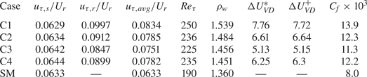
Wall friction comparison. Here,  $u_{\tau,s}=\sqrt {\tau _{w,s}/\rho _r}$ and $u_{\tau,r}=\sqrt {\tau _{w,r}/\rho _r}$, where $\tau _{w,s}=-\mu _r({{\rm d}\langle \bar {u}\rangle }/{{\rm d} y})\vert _{y=2\delta }$ is wall shear stress on the smooth side and $\tau _{w,r}=({1}/{A_t})\int _{V_f}\bar {f}_1 \,\text {d}v -\tau _{w,s}$ is that on the rough side (obtained from momentum balance); ${Re}_\tau =\rho _r u_{\tau,avg} \delta /\mu _r$, $C_f=2(u_{\tau,avg}/U_r)^2$, $u_{\tau,avg}^2=(u_{\tau,s}^2+u_{\tau,r}^2)/2$, $\rho _w$ is the density value at $y=0$, and $\Delta U^*_{VD}$ and $\Delta U^+_{VD}$ are the roughness functions associated with the van Driest transformed velocities.
2.4. Validation of the numerical method and the IB method
The numerical method is validated by simulating a smooth-wall supersonic turbulent channel flow at  $M=1.5$ and ${Re}=3000$. The same set-up was employed by Coleman et al. (Reference Coleman, Kim and Moser1995), which is used here as the benchmark study.
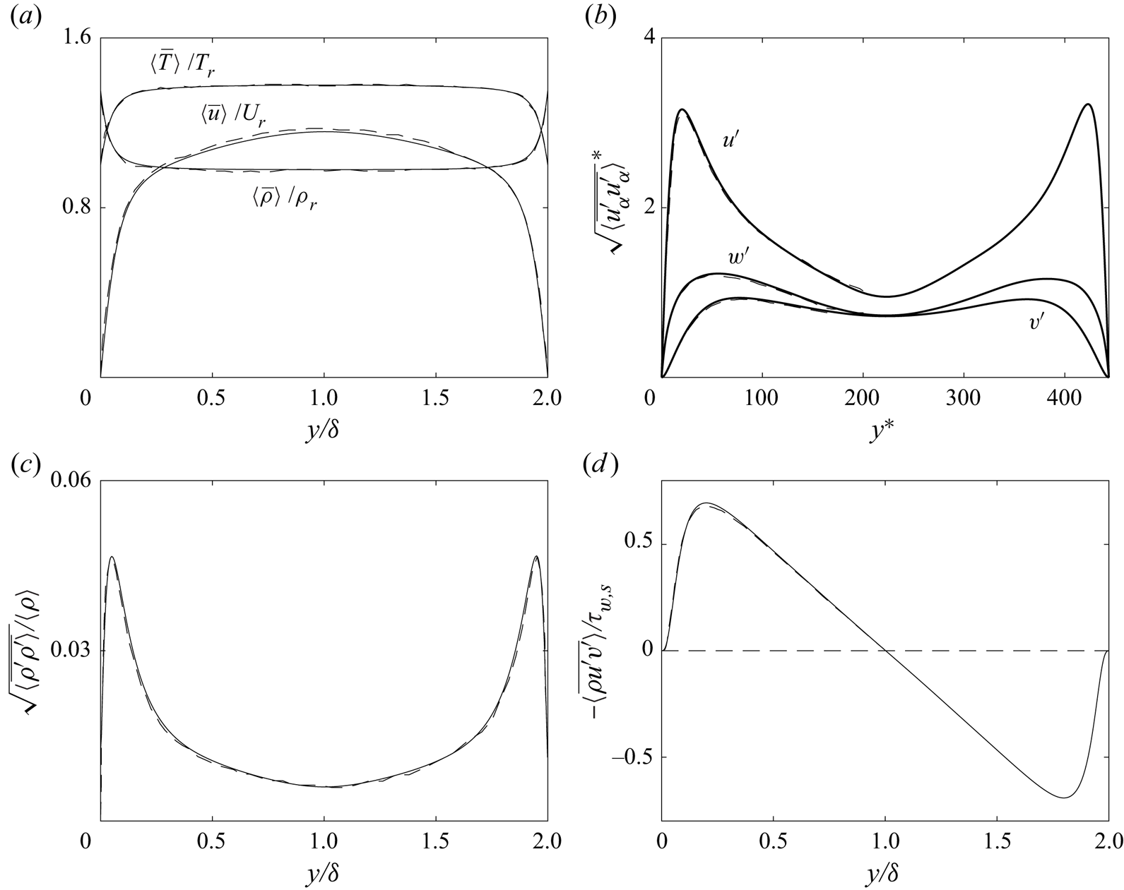
Figure 2 compares mean and turbulence statistics of the present simulation with those of Coleman et al. (Reference Coleman, Kim and Moser1995). The two simulations are in a good agreement for mean velocity, density and temperature, as well as for Reynolds stresses and density variance. This verifies the numerical solver.
Profiles of mean and turbulence variables for the smooth-wall flow at  ${Re}=3000$ and $M=1.5$: —— present simulation, – – – Coleman, Kim & Moser (Reference Coleman, Kim and Moser1995). (a) Mean values of temperature, streamwise velocity and density, (b) r.m.s. of turbulent velocities (no summation over Greek indices, $*$ denotes normalization in wall units using $\tau _{w,s}=\mu _r\langle {{\rm d}\bar {u}}/{{\rm d} y}\vert _w\rangle$ and $\rho _w$), (c) r.m.s. of density and (d) Reynolds shear stress.
To validate the proposed IB method, we simulated case C1 in two ways: one using the IB method and the other solving the conventional NS equations on a body-fitted mesh set-up. The contour of level-set function  $\psi$ for the IB method and the mesh of the conformal set-up are compared in figure 3. The contour line corresponding to $\psi =0$ represents well the fluid–solid interface.
Contour of level set  $\psi$, ranging from $-1$ (blue) to $+1$ (yellow) used for the IB method (a), and mesh used for the conformal set-up (b), both for case C1. In panel (a) the solid white and black lines indicate, respectively, the exact roughness height as in (2.9) and the iso-line of $\psi =0$ obtained from the level-set equation (2.4); the difference between the two lines is one grid point maximum. The inset in (a) zooms in to show the interface.

Figure 4 compares the results obtained using the IB method and those using a body-fitted mesh, in terms of various mean and turbulence variables, including mean profiles of velocity, temperature and density, Reynolds stresses and variance of temperature. All plots show a good agreement between the two simulations. One notices, however, slight differences (approximately 5 %) in the  $u'''$ r.m.s. profiles near the crest elevation of roughness at $y^+= 25$. This is probably due to the different meshes used in the IB simulation and the conformal one and the interpolation scheme used in the conformal case to convert fluid fields to the Cartesian coordinates before the statistics were calculated. Overall, these results validate the use of the present IB method to characterize single-point statistics of mean flow and turbulence. See supplementary movie 1 available at https://doi.org/10.1017/jfm.2022.1049 for flow visualizations for case C1 with the IB method.
Mean and turbulence variables for case C1, simulated using the IB method (——) and the conformal mesh (– – –): mean temperature, streamwise velocity and density (a), r.m.s. of velocity components in plus units (roughness side, b), time and spanwise average of velocity and temperature at the roughness crest and valley locations (c, crest in blue and valley in black) and r.m.s. of temperature (d). In (d), note that temperature r.m.s. is theoretically zero at the roughness trough ( $y=0$); the intrinsic-averaged value in $y\approx 0$ region for the IBM case, however, fluctuates due to the limited fluid area. This region is removed from the plot. The vertical dot-dash lines show $y=k_c$. Superscript $+$ denotes normalization in wall units using $u_{\tau,r}$ (tabulated in table 2) and $\rho _r$.

3. Results
3.1. Visualizations of the instantaneous and averaged fields
Instantaneous vortical structures are visualized using iso-surfaces of the  $Q$-criterion (Chong, Perry & Cantwell Reference Chong, Perry and Cantwell1990) in figure 5. Modifications of the near-wall turbulence on the rough-wall side are noticeable. The main difference between the effects of different roughness geometries is the shock patterns shown by the instantaneous numerical schlieren images (figure 6). These patterns are also persistent in time as shown by time- and spanwise-averaged $\boldsymbol {\nabla }\boldsymbol {\cdot }\boldsymbol {u}$ (figure 7). Both figures show that 2-D surfaces (cases C1 and C2) induce strong shocks that reach the upper wall and are reflected back to the domain after impingement. The shock patterns exhibit the same wavelength of the roughness geometries, and influence the flow properties in the whole channel. This is obvious in the contours of instantaneous temperature fields in figure 8, where temperature periodically changes in the compression and expansion regions associated with roughness geometries in C1 and C2. For 3-D cases the embedded shocks are weaker and, consequently, replaced by the small-scale shocklets.
Isosurfaces of  $Q=3$ (in blue, normalized by $U_r$ and $\delta$) for all rough cases. The grey isosurfaces show the roughness surfaces.

Numerical schlieren images, showing contours of instantaneous  $\log {\vert \boldsymbol {\nabla }\rho \vert }$. For a better visualization the contour ranges are chosen differently for different cases. Here, $\boldsymbol {\nabla }\rho$ is normalized by $\rho _r$ and $\delta$.

Contours of  $\boldsymbol {\nabla }\boldsymbol {\cdot } \boldsymbol {u}$ averaged in time and spanwise direction. All normalized by $U_r$ and $\delta$. To calculate the spanwise-averaged values, intrinsic averaging was performed along the spanwise direction at each $(x,y)$ point. An $x$ slice of the corresponding rough surface is shown in each panel.

Contours of instantaneous  $T$, normalized by $T_r$.

3.2. Mean and turbulence variables
First, the values of frictional velocities on the smooth and rough sides as well as the frictional Reynolds number  ${Re}_\tau$ and drag coefficient $C_f$ are tabulated in table 2 for all cases. On the rough-wall side, the wall friction includes both viscous and pressure drag components. Due to differences in wall friction generated by roughnesses of different geometries, ${Re}_\tau$ varies from 190 to 250. Yet, the flows are all low-Reynolds-number ones; the differences in shock features and flow statistics (discussed thoroughly below) are thus likely a result of the change in roughness geometry, instead of the change in friction Reynolds number.
The comparison shows that, as expected, the wall friction on the rough-wall side is higher than that on the smooth-wall side for all cases. Overall, a 2-D roughness generates higher friction than a 3-D one of the same height. This is consistent with observations in incompressible flows (e.g. by Volino et al. Reference Volino, Schultz and Flack2011) that 2-D roughness affects turbulence more strongly due to the larger length scale (in  $z$) that is imparted to the flow. In addition, results show that for 3-D roughnesses a higher friction is obtained for a shorter wavelength (or higher roughness slope), which is also consistent with observations in incompressible flows (Napoli, Armenio & De Marchis Reference Napoli, Armenio and De Marchis2008). Between the two 2-D rough surfaces, however, the one with a higher slope (C2) yields a lower wall friction. As will be shown later in § 3.3, this appears to be a result of stronger turbulent mixing above the rough surface in C1 than in C2, due to regions with more intense compression (those with strong negative values of $\boldsymbol {\nabla }\boldsymbol {\cdot }\boldsymbol {u}$, figure 7) in which strong turbulent kinetic energy (TKE) production and redistribution take place. These observations indicate that, in fully developed supersonic rough-wall flows, the dependency of the wall friction on roughness geometry is more complex than in incompressible flows, due to compressibility effects. Future systematic studies with a wide range of different rough surfaces are needed to detail the dependences of shocks on roughness height and geometry, and analyses of near-wall momentum balance are needed to further understand changes of the flow.
Figure 9 compares profiles of the mean and turbulence quantities between different cases. The mean streamwise velocity (figure 9a) and density (not shown) are both weakly dependent on the roughness geometry across the channel, except for the region near the rough wall. This is because the normalization using the bulk values ( $U_r$ and $\rho _r$) absorbs major differences in the velocity and density profiles in the bulk part of the channel. The mean temperature values (figure 9c), on the other hand, differ across the channel for different roughness topographies. The mean temperature is higher for 2-D roughness cases (C1 and C2) compared with the 3-D ones (C3 and C4) and the smooth case (SM). Here, the temperature is normalized by the wall value, $T_w$, which does not absorb the differences in the core region. It is established (Anderson Reference Anderson1990, chapter 3) that shock waves result in entropy generation, because of strong viscous effects and thermal conduction in large gradients regions. The stronger shocks in the 2-D roughness cases involve more entropy in the domain than in the 3-D cases. As a result, the irreversible heat generation is more intense for these cases, leading to higher temperature values.
Mean and turbulence variables for cases C1 (——, thick solid line), C2 (– – –), C3 (– - –), C4 (- - -) and SM (——): profiles of the double-averaged streamwise velocity (a), r.m.s. of velocities in plus units (roughness side, b), double-averaged temperature (c) and r.m.s. of temperature (d). In (d), note that temperature r.m.s. is theoretically zero at the roughness trough ( $y=0$); the intrinsic-averaged value in $y\approx 0$ region, however, fluctuates due to the limited fluid area. This region is removed from the plot.

The r.m.s. of the three  $u'''_i$ fluctuation components are plotted in figure 9(b) in wall units. For rough cases, it shows that roughness effects are mostly confined to a near-wall region; outside this region the differences between profiles for different rough surfaces are smaller for all velocity components. This is similar to the concept of the roughness sublayer, defined as the near-wall layer where turbulence statistics in wall units vary with the wall condition (Flack, Schultz & Connelly Reference Flack, Schultz and Connelly2007), in an incompressible turbulent flow bounded by rough wall. Near the wall, the $v'''$ and $w'''$ components are similar among all cases, whereas the $u'''$ components in 3-D cases display a peak closer to the wall than their 2-D counterparts. Similar phenomena were observed for incompressible flow; it was explained as a result of a thicker roughness sublayer over a 2-D roughness (Volino et al. Reference Volino, Schultz and Flack2011), leading to a peak farther from the smooth-wall peak elevation at $y^+\approx 15$. The fact that the turbulence intensities in wall units do not collapse perfectly in the outer layer (i.e. the region above the roughness sublayer) among all cases indicates that the wall similarity (or ‘outer layer similarity’, Schultz & Flack Reference Schultz and Flack2007) of Townsend (Reference Townsend1976) does not apply. The wall similarity hypothesis (primarily describing incompressible flows) states that, at high Reynolds number and with very small roughness compared with $\delta$, turbulent statistics outside the roughness sublayer are independent of wall roughness, except for its scaling on the friction velocity. Given the relatively low Reynolds number and large roughness ( $k_c/\delta = 0.1$) in the present cases, exact wall similarity is not expected. In addition, in current supersonic flows roughness is shown to directly affect outer layer turbulence through its effect on shocks that extend to the core region of the channel flow (figures 6 and 7).
The profiles of temperature r.m.s. in figure 9(d) show that the intensity of temperature fluctuations far from the wall depends strongly on the roughness geometry. For 2-D rough surfaces, the variations of curve shape in the bulk of the channel are associated with the shock patterns in the domain. Temperature varies significantly near the locations where the shock waves coincide and form nodes of shock diamonds (i.e. the nodes away from walls). These shock diamonds are also visible in figures 6, 7 and 8 (C1 and C2). For 3-D cases the shock diamonds are weak or non-existent. Therefore, the curves of temperature r.m.s. in 3-D cases are smooth in the core region.
Figure 10 compares the mean velocity profiles in inner units. The law of the wall for mean velocity scaled in this way refers to the universal logarithmic profile in regions between  $50\delta _\nu \lesssim y\lesssim 0.2\delta$ (where $\delta _\nu$ is the viscous length scale) on a smooth wall. On a rough wall, incompressible flow studies showed that the logarithmic profile still exists, with its lower extent shifted to the top of roughness sublayer. Both roughness and compressibility were found to influence the law of the wall through their effects on the inner units. Specifically, roughness shifts the logarithmic profiles downward for an amount $\Delta U^+$ (called roughness function) with respect to a smooth-wall flow (Nikuradse Reference Nikuradse1933). This has been observed for a wide range of roughness topographies (Raupach et al. Reference Raupach, Antonia and Rajagopalan1991; Leonardi, Orlandi & Antonia Reference Leonardi, Orlandi and Antonia2007; Schultz & Flack Reference Schultz and Flack2007; Busse, Thakkar & Sandham Reference Busse, Thakkar and Sandham2017; Forooghi et al. Reference Forooghi, Stroh, Magagnato, Jakirlic and Frohnapfel2017; Womack et al. Reference Womack, Volino, Meneveau and Schultz2022, to name a few).
Law of the wall. Profiles of mean velocities transformed using (a) original van Driest transformation (3.1) and (b) a modified van Driest transformation (3.2). Cases C1 (——, thick solid line), C2 (– – –), C3 (– - –), C4 (- - -) and SM (——). Solid magenta lines (——) show slope of  $1/\kappa$, where $\kappa =0.41$ is the von Kármán constant. In (a) results of Coleman et al. (Reference Coleman, Kim and Moser1995) (– – –, red) and Foysi, Sarkar & Friedrich (Reference Foysi, Sarkar and Friedrich2004) (- - -, red) for smooth-wall flows are provided for comparison, and the blue solid line is same as the C1 profile in (b). Here, $\Delta U^*_{VD}$ and $\Delta U^+_{VD}$ are roughness functions for case C1.

For compressible flows, finding appropriate inner velocity, length, density and viscosity scales that result in universal law of the wall is an active subject of research for smooth-wall flows (Morkovin Reference Morkovin1962; Volpiani et al. Reference Volpiani, Iyer, Pirozzoli and Larsson2020, among many others). The complexities stem from significant variations in density, viscosity and heat transfer across the boundary layer that need to be accounted for. Here, we plot density-transformed mean velocity profiles, introduced by Van Driest (Reference Van Driest1951). The approach has been shown to collapse mean velocity profiles for smooth-wall flows at different Mach numbers (Guarini et al. Reference Guarini, Moser, Shariff and Wray2000; Lagha et al. Reference Lagha, Kim, Eldredge and Zhong2011; Trettel & Larsson Reference Trettel and Larsson2016). The original van Driest transformation reads as
 \begin{equation} U^*_{VD}=\int_0^{\langle\bar{u}\rangle^*}\left(\frac{\langle\bar{\rho}\rangle}{\rho_w}\right)^{1/2} \,\text{d}\langle\bar{u}\rangle^*, \end{equation}
where superscript  $*$ denotes normalization using $\tau _{w,r}$, $\rho _w=\langle \bar {\rho }\rangle \vert _{y=0}$ and $\mu _r$. The results are plotted in figure 10(a). The profiles of Coleman et al. (Reference Coleman, Kim and Moser1995) and Foysi et al. (Reference Foysi, Sarkar and Friedrich2004) for smooth-wall flows ( $M=1.5$ and ${Re}=3000$) are also compared. The present SM profile matches very well with the reference data. We also employ a modified van Driest transformation, where all density scales are normalized by $\rho _r$ instead of $\rho _w$. The modified van Driest transformation is
 \begin{equation} U^+_{VD}=\int_0^{\langle\bar{u}\rangle^+}\left(\frac{\langle\bar{\rho}\rangle}{\rho_r}\right)^{1/2} \,\text{d}\langle\bar{u}\rangle^+, \end{equation}
where superscript  $+$ denotes normalization using $\tau _{w,r}$, $\rho _r$ and $\mu _r$. The results are plotted in figure 10(b). Since both $\rho _w$ and $\rho _r$ are of the order of unity, $U^*_{VD}$ and $U^+_{VD}$ are not significantly different (comparing the solid blue and black lines in figure 10(a) for case C1). A constant displacement height $d=0.8k_c$ is chosen for the rough cases in figure 10. All rough-wall profiles in figure 10 show a downward shift ( $\Delta U_{VD}$) with respect to the smooth wall due to higher wall friction, similar to incompressible flows. The magnitudes of $\Delta U^*_{VD}$ and $\Delta U^+_{VD}$ are measured at $(y-0.8k_c)^*=100$ and $(y-0.8k_c)^+=100$, respectively, and tabulated in table 2. The two different transformations give virtually the same roughness functions, which are larger for 2-D rough cases than 3-D ones and display the same comparison as that of $C_f$ among all cases (table 2). These observations suggest that the discussions in the literature concerning equilibrium incompressible rough-wall drag laws may be extendable to equilibrium supersonic rough-wall flows, when the van Driest types of transformation are employed, as long as the Mach number is not too high. The latter may be necessary as the essential dynamics of turbulence in equilibrium compressible flows is expected to remain similar to its incompressible counterparts, if the Mach number is not high enough to yield prevailing compressibility effects (Morkovin Reference Morkovin1962). Also, one notices in figure 10 that $1/\kappa$ (where $\kappa \approx 0.41$ being the von Kármán constant) is still a good approximation for the slopes of both $U^*_{VD}$ and $U^+_{VD}$ profiles for the present rough cases, although with minor noticeable variations.
3.3. Budgets of the Reynolds stresses
The transport equation for various components of the Reynolds stress tensor in a compressible flow reads as (Vyas, Yoder & Gaitonde Reference Vyas, Yoder and Gaitonde2019)
 \begin{align} \frac{\partial}{\partial t}(\overline{\rho u_i''u_j''}) &= \mathcal{C}_{ij}+\mathcal{P}_{ij} +\mathcal{D}_{ij}^{M}+\mathcal{D}_{ij}^{T}\nonumber\\ &\quad + \mathcal{D}_{ij}^{P}+{\varPi}_{ij}+{\epsilon}_{ij}+\mathcal{M}_{ij}, \end{align}
where  $i$,
$i$,  $j = \{1, 2, 3\}$ and $\mathcal {C}$, $\mathcal {P}$, $\mathcal {D}^M$, $\mathcal {D}^T$, $\mathcal {D}^P$, $\varPi$, $\epsilon$ and $\mathcal {M}$, are, respectively, mean convection, production, molecular diffusion, turbulent diffusion, pressure diffusion, pressure strain, dissipation and turbulent mass flux terms, and are defined as
 \begin{equation} \left.\begin{gathered} \mathcal{C}_{ij}={-}\frac{\partial}{\partial x_k}(\overline{\rho u''_iu''_j}\tilde{u}_k),\\ \mathcal{P}_{ij}={-}\overline{\rho u''_iu''_k}\frac{\partial\tilde{u}_j}{\partial x_k} -\overline{\rho u''_ju''_k}\frac{\partial\tilde{u}_i}{\partial x_k},\\ \mathcal{D}_{ij}^M= \frac{\partial}{\partial x_k}(\overline{u''_i \tau_{kj}}+\overline{u''_j \tau_{ki}}),\\ \mathcal{D}_{ij}^T={-}\frac{\partial}{\partial x_k}(\overline{\rho u''_i u''_j u''_k}),\\ \mathcal{D}_{ij}^P={-}\frac{\partial}{\partial x_k}(\overline{p'u''_i}\delta_{jk}+\overline{p'u''_j}\delta_{ik}),\\ \varPi_{ij}= \overline{p'\left(\frac{\partial u''_i}{\partial x_j}+\frac{\partial u''_j}{\partial x_i}\right)},\\ \epsilon_{ij}={-} \overline{\tau_{ki}\frac{\partial u''_j}{\partial x_k}} - \overline{\tau_{kj}\frac{\partial u''_i}{\partial x_k}},\\ \mathcal{M}_{ij}= \overline{u''_i}\left(\frac{\partial\overline{\tau}_{kj}}{\partial x_k}-\frac{\partial \bar{p}}{\partial x_j}\right) +\overline{u''_j}\left(\frac{\partial\bar{\tau}_{ki}}{\partial x_k}-\frac{\partial \bar{p}}{\partial x_i}\right). \end{gathered}\right\} \end{equation}
 The budget terms are calculated for all non-zero components of the Reynolds stress tensor and for TKE. The budget balance of the transport equation of  $\langle \overline {\rho u''_iu''_j}\rangle$ is denoted as $B_{ij}$. Figures 11 and 12 show wall-normal profiles of the spatial-averaged budget terms of TKE and $\langle \overline {\rho u''u''}\rangle$, respectively. Both normalizations by the reference units ( $\rho _r$, $U_r$ and $\delta$) and by the wall units ( $\rho _r$, $u_{\tau,r}$ at bottom wall and $\mu _r$) are used. The residual of the calculated budget balance, $\sigma$, is presented; it is less than 1 % of the maximum value of the shear production $\mathcal {P}$ in all cases. This suggests that the budget terms are calculated correctly and that the numerical dissipation (as a result of both the solver's flux-splitting procedure and the IBM) is small for estimation of the budget terms.
Budget balances of TKE. All terms are double averaged in time and in the  $x$–
$x$– $z$ plane. They are normalized by the outer units $\rho _r$, $U_r$ and $\delta$ for the panels, and wall ( $+$) units $\rho _r$, $u_{\tau,r}$ and $\mu _r$ in the insets. The vertical dash lines show $y=k_c$.

Budget balances of B11. All terms are double averaged in time and the  $x$–
$x$– $z$ plane. They are normalized by the outer units $\rho _r$, $U_r$ and $\delta$ for the panels, and wall ( $+$) units $\rho _r$, $u_{\tau,r}$ and $\mu _r$ in the insets. Panel ( f) compares the production and pressure-strain terms of all cases: C1 (——, thick solid line), C2 (– – –), C3 (– - –), C4 (- - -) and SM (——). The vertical dash lines show $y=k_c$.

Comparing the smooth- and rough-wall cases, the main differences are seen near the wall. Specifically, molecular diffusion and viscous dissipation are non-zero on the smooth wall, whereas they are zero on the bottom of the rough wall attributed to a quiet region without turbulence at the root of the roughness elements. Overall, both production and pressure-strain term on a rough-wall peak at elevations near the roughness crest, independent of the smooth-wall peak elevations.
Among the rough cases, the magnitudes of the budget terms normalized by the reference values are shown to be modified by the roughness topography, with the 2-D surfaces producing higher magnitudes than the 3-D ones. Two important terms,  $\mathcal {P}_{11}$ and $\varPi _{11}$ are compared in figure 12 among all cases. The comparison among the magnitudes of both $\mathcal {P}_{11}$ and $\varPi _{11}$ displays the same trend as those of the temperature profiles (figure 9c) and $C_f$ (table 2), suggesting that an enhancement of turbulence processes augments temperature and hydrodynamic drag. For further explanations, the contours of $\mathcal {P}_{11}$ in an $(x,y)$ plane are shown in figure 13 to compare the spatial distribution of this term. It shows that 2-D roughness elements lead to stronger turbulence production downstream of each roughness peak than the 3-D roughnesses. This is probably because the 2-D roughnesses induce organized recirculation regions that are aligned in $z$ and stronger shear layers around the recirculation regions. In addition, turbulence production above a 2-D roughness is enhanced by the strong mutual interaction between shock waves. In 2-D roughness cases the regions where two oblique shock waves impinge together (figure 7) are associated with enhanced turbulence production, whether it is on the rough- or smooth-wall side.
Contours of  ${\mathcal {P}}_{11}$ normalized using $\rho _r$, $U_r$ and $\delta$. An $x$ slice of the corresponding rough surface is shown in each panel.

The effect of shocks on turbulence is an important phenomenon and represents a fundamental difference between supersonic and subsonic turbulent flows over rough walls – for incompressible flows most of the roughness effects are confined to near-wall regions and the outer layer is expected to be independent of the wall condition (except for the scaling of outer-layer statistics on the friction velocity), also known as outer layer similarity (Townsend Reference Townsend1976; Raupach et al. Reference Raupach, Antonia and Rajagopalan1991; Schultz & Flack Reference Schultz and Flack2007). However, for the supersonic cases herein, the effects of wall roughness propagate across the channel and modify turbulence production in the upper wall region via the generated oblique shocks. The same process occurs on the rough-wall side, where the reflected shocks from the smooth-wall side impinge back to the rough wall and enhance the turbulence production in these regions. In other words, turbulence processes on both walls depend on the interaction of shocks, which are themselves dependent on the roughness topography. This indicates that outer-layer similarity does not apply to such supersonic channel flows, at least for the Reynolds number, Mach number and wall roughness in the present simulations. The far-reaching effect of surface details may be of potential use in flow and turbulence control.
3.4. Conditional analysis
In this section, contributions from regions of either expansion, compression or solenoidal flow to the overall TKE production is analysed and compared among all cases. The velocity divergence ( $\boldsymbol {\nabla }\boldsymbol {\cdot }\boldsymbol {u}$) is used as a measure of compressibility. Large magnitudes of $\boldsymbol {\nabla }\boldsymbol {\cdot }\boldsymbol {u}$ correspond to regions of strong compression or expansion immediately before and after a shock wave.
Figure 14(a–e) shows the probability density function (p.d.f.) of  $\boldsymbol {\nabla }\boldsymbol {\cdot }\boldsymbol {u}$, evaluated at each $y$-location and normalized to yield the maximum value of 1. There $\mathcal {D}$ denotes values taken by $\boldsymbol {\nabla }\boldsymbol {\cdot }\boldsymbol {u}$. To calculate the p.d.f. at all $y$ elevations, the bin width is chosen as a constant 0.2 in reference units, with $(\boldsymbol {\nabla }\boldsymbol {\cdot }\boldsymbol {u})_{max}=40$, $(\boldsymbol {\nabla }\boldsymbol {\cdot }\boldsymbol {u})_{min}=-40$. For the 2-D roughness cases (C1 and C2), velocity divergence values far from the walls scatter towards much larger magnitudes than those near the wall, while they remain in the vicinity of zero for the 3-D and smooth-wall cases. This is a quantitative comparison showing the more significant compressibility effects in the 2-D roughness cases owing to the strong oblique shock waves away from the walls. It also confirms that the 3-D roughnesses do not induce strong compressibility effects in the flow, similar to what happens in the smooth-wall case.
Probability density functions of velocity divergence evaluated at all  $y$ values (a–e), conditional expectations of TKE shear production given velocity divergence $E(\mathcal {P}_{TKE} | \boldsymbol {\nabla }\boldsymbol {\cdot }\boldsymbol {u}=\mathcal {D})$ ( f–j) and their respective products (k–o). Panels (a–e) are normalized to yield the maximum value of 1.

Next, the TKE production conditionally averaged based on velocity divergence,  $E(\mathcal {P}_{TKE} | \boldsymbol {\nabla }\boldsymbol {\cdot }\boldsymbol {u}=\mathcal {D})$, evaluated at each $y$, is shown in figure 14( f–j). In all cases, regions with large magnitudes of $\mathcal {D}$ contribute significantly to $\mathcal {P}_{TKE}$, both near and far from the wall. This is prominent in the 2-D roughness cases and, to a lower extent, in the 3-D roughness and smooth-wall cases. Although high magnitude $\mathcal {D}$ events are associated with significant $\mathcal {P}_{TKE}$, their probability of occurrence is low according to the p.d.f. of $\boldsymbol {\nabla }\boldsymbol {\cdot }\boldsymbol {u}$. To assess the distribution of the actual amount of $\mathcal {P}_{TKE}$ attributed to regions of different $\boldsymbol {\nabla }\boldsymbol {\cdot }\boldsymbol {u}$ values, the product between p.d.f. of $\boldsymbol {\nabla }\boldsymbol {\cdot }\boldsymbol {u}$ and $E(\mathcal {P}_{TKE} | \boldsymbol {\nabla }\boldsymbol {\cdot }\boldsymbol {u}=\mathcal {D})$ is plotted in figure 14(k–o), for each $\mathcal {D}$ and at each $y$. Results show that the majority of TKE production comes from low-compressibility regions, due to their high probabilities of occurrence. The 2-D roughnesses lead to larger fractions of TKE production from negative- $\mathcal {D}$ (or compression) events.
To quantitatively compare individual contributions from regions with different types of compressibility to the overall TKE production, figure 15 shows profiles of  $\mathcal {P}_{TKE}$ and $\epsilon _{TKE}$ conditioned on three types of events: compression events (where ${\boldsymbol {\nabla }\boldsymbol {\cdot }\boldsymbol {u}}/{U_r/\delta }\leqslant -0.15$), solenoidal events ( $-0.15<{\boldsymbol {\nabla }\boldsymbol {\cdot }\boldsymbol {u}}/{U_r/\delta }<0.15$) and expansion events ( ${\boldsymbol {\nabla }\boldsymbol {\cdot }\boldsymbol {u}}/{U_r/\delta }\geqslant 0.15$). The threshold value 0.15 is chosen from figure 14(e) as approximately the maximum magnitude reached in the smooth case. In other words, for the purpose of the conditional analysis, the smooth-wall flow at the present Mach number is considered only weakly compressible (relative to the rough-wall cases). For the 3-D roughnesses and smooth-wall cases, the solenoidal events are shown responsible for almost all of the TKE production (and dissipation rate). However, for 2-D surfaces the compression events contribute as much as 30 % on these processes near the wall, while the contribution from expansion events is about 5 %; far from the wall ( $y/\delta > 0.2$), the total contribution from compression events overtakes that from solenoidal ones. This indicates that the shocks, dependent on the roughness topography, dynamically influences the turbulent flow across the channel. For further understanding of how roughness geometry affects the Reynolds stress balance, future studies are needed to characterize the dilatation terms (i.e. pressure dilatation and dilatation dissipation, Sarkar et al. Reference Sarkar, Erlebacher, Hussaini and Kreiss1991), which are normally small at present Mach and Reynolds numbers in channel flow with smooth walls but may be significant on rough walls due to the presence of shocks.
Profiles of spatially averaged  $\mathcal {P}_{ii}$ (——) and $\epsilon _{ii}$ (– – –) conditioned on various types of compressibility. Quantities are normalized using $\rho _r$, $U_r$ and $\delta$.

4. Concluding remarks
Effects of surface roughness and its topography on compressible turbulent flows were characterized based on simulations of four supersonic channel flows at  $M=1.5$ and the bulk Reynolds number ${Re}=3000$ with top smooth walls and four different roughness geometries on the bottom walls. A baseline smooth-wall channel was also simulated. A modified level-set/VOF IB method was used to impose the BCs of velocity and temperature on the surface of roughness. The method was validated in terms of mean and turbulence statistics against a companion conformal mesh simulation. The four roughnesses include two 2-D and two 3-D sinusoidal surfaces. The surfaces shared the same peak-to-trough height (of 10 % channel half-height) but differed in the surface wavelength.
Results showed significant modifications of turbulence across the channel by the roughness. Roughness generates a distribution of oblique shocks in connection to the roughness geometry. These shocks are much stronger on the 2-D roughnesses; they reach across the channel, reflected back from the smooth-wall side, and interact to form shock diamonds. Such strong shock patterns are absent in the smooth-wall channel.
The strong shocks generated by the 2-D roughnesses lead to stronger irreversible heat generation and higher temperature values in the bulk of the channel, than in the 3-D roughness cases. Roughness on one side of the channel enhances TKE production on both sides. Conditional analyses based on local compressibility showed that, although high-compressibility regions are associated with significantly enhanced local TKE production, the probability of occurrence of such regions is low and dependent on the roughness geometry. For the 2-D roughness cases up to 30 % of TKE production and dissipation near the rough wall (as well as most of the outer-layer production and dissipation) occur in compression regions. However, for the 3-D roughness and smooth-wall cases these processes are almost all associated with relatively solenoidal events.
This work identifies the mechanism through which wall roughness and its texture affect a compressible turbulence. It demonstrates that in supersonic channels the roughness effects can propagate throughout the boundary layer. In this case, the outer-layer similarity established for incompressible flows does not apply. This work focuses on flow statistics. To fully characterize roughness effects in compressible flows, future studies on spectral and structural effects, scaling and variable density effects are needed.
Supplementary movie
Supplementary movie is available at https://doi.org/10.1017/jfm.2022.1049.
Funding
Computational support was provided by Michigan State University's Institute for Cyber-Enabled Research.
Declaration of interests
The authors report no conflict of interest.


 Open access