


1. Introduction
The transport and deposition of tiny (cohesive) particles in turbulent flows play important roles in many engineering, environmental and medical systems. Examples include dry powder inhalers for drug delivery (Begat et al. Reference Begat, Morton, Staniforth and Price2004; Yang, Wu & Adams Reference Yang, Wu and Adams2013, Reference Yang, Wu and Adams2015), dust ingestion in gas turbine engines (Batcho et al. Reference Batcho, Moller, Padova and Dunn1987; Dunn, Baran & Miatech Reference Dunn, Baran and Miatech1996; Bons, Prenter & Whitaker Reference Bons, Prenter and Whitaker2017; Sacco et al. Reference Sacco, Bowen, Lundgreen, Bons, Ruggiero, Allen and Bailey2018) and fluidized bed reactors (Mikami, Kamiya & Horio Reference Mikami, Kamiya and Horio1998; van der Hoef et al. Reference van der Hoef, van Sint Annaland, Deen and Kuipers2008; Mahecha-Botero et al. Reference Mahecha-Botero, Grace, Elnashaie and Lim2009; Pan et al. Reference Pan, Chen, Liang, Zhu and Luo2016). Micrometre-sized particles tend to form aggregates owing to inter-particle cohesion. The dynamical evolution and morphology of these aggregates involve a complex interplay between turbulent stresses and inter-particle cohesive forces. As a result, particle clumping can arise under various circumstances, which is known to compromise the performance of the aforementioned systems. For example, agglomeration has been shown to significantly deteriorate the delivery efficiency of drug particles (Begat et al. Reference Begat, Morton, Staniforth and Price2004), accelerate turbine blade erosion in gas turbine engines (Grant & Tabakoff Reference Grant and Tabakoff1975; Hamed, Tabakoff & Wenglarz Reference Hamed, Tabakoff and Wenglarz2006) and defluidize two-phase reactors (Mikami et al. Reference Mikami, Kamiya and Horio1998; Cocco et al. Reference Cocco, Shaffer, Hays, Karri and Knowlton2010). Of particular interest to the present study is turbulence-induced breakup of fine particulate aggregates.
Several mechanisms are responsible for particle deagglomeration in a flow field. Breakup can be induced by inertial stresses (Kousaka et al. Reference Kousaka, Okuyama, Shimizu and Yoshida1979; Higashitani, Iimura & Sanda Reference Higashitani, Iimura and Sanda2001), rotary stresses (Sonntag & Russel Reference Sonntag and Russel1987; Jarvis et al. Reference Jarvis, Jefferson, Gregory and Parsons2005; Fanelli, Feke & Manas-Zloczower Reference Fanelli, Feke and Manas-Zloczower2006a,Reference Fanelli, Feke and Manas-Zloczowerb; Zeidan et al. Reference Zeidan, Xu, Jia and Williams2007; Mousel & Marshall Reference Mousel and Marshall2010) or turbulent stresses (Bache Reference Bache2004; Wengeler & Nirschl Reference Wengeler and Nirschl2007; Bäbler, Morbidelli & Baldyga Reference Bäbler, Morbidelli and Baldyga2008; Weiler et al. Reference Weiler, Wolkenhauer, Trunk and Langguth2010). Several models have recently been developed for deagglomeration due to rotary stress in simple shear flows (Dizaji, Marshall & Grant Reference Dizaji, Marshall and Grant2019; Ruan, Chen & Li Reference Ruan, Chen and Li2020; Vo et al. Reference Vo, Mutabaruka, Nezamabadi, Delenne and Radjai2020). The mechanisms responsible for deagglomeration in turbulence, however, are more complicated and less established. Weiler et al. (Reference Weiler, Wolkenhauer, Trunk and Langguth2010) developed a model of critical shear stress for instantaneous breakage as a function of aggregate size and the mean cohesive force. However, aggregates often break up progressively from the surface, and the critical stress at the vicinity of the aggregate is not always directly available, especially in course-grained simulations where subgrid-scale stresses are not resolved such as in Reynolds-averaged Navier–Stokes (RANS) frameworks.
The major challenge in numerically investigating the breakage of cohesive particles is properly resolving the wide range of length and time scales at play. One common approach is to couple Lagrangian particle tracking with a mean flow field obtained from RANS. The turbulent dispersion of particles is often modelled in a stochastic manner. This approach has been widely used for particle ingestion in gas turbine engines (Grant & Tabakoff Reference Grant and Tabakoff1975; Hamed et al. Reference Hamed, Tabakoff and Wenglarz2006; Bons et al. Reference Bons, Prenter and Whitaker2017). Despite its low computational cost, Lagrangian particle tracking coupled with RANS has been shown to under-predict turbulent dispersion and deposition of particles compared with experiments (Whitaker, Prenter & Bons Reference Whitaker, Prenter and Bons2015), especially near boundary layers (Rybalko, Loth & Lankford Reference Rybalko, Loth and Lankford2012; Forsyth, Gillespie & McGilvray Reference Forsyth, Gillespie and McGilvray2018). In contrast, particle-resolved direct numerical simulation (PR-DNS) has been applied to fully capture the flow field and particle interactions (Uhlmann Reference Uhlmann2008; Vowinckel et al. Reference Vowinckel, Biegert, Luzzatto-Fegiz and Meiburg2019a,Reference Vowinckel, Withers, Luzzatto-Fegiz and Meiburgb). While PR-DNS is highly accurate, it is limited to small physical systems owing to its high computational cost.
Alternatively, the Eulerian–Lagrangian method tracks individual particles and solves the fluid phase on an Eulerian mesh with grid spacing larger than the particle diameter. It is capable of capturing detailed particle–particle interactions and particle–fluid coupling with moderate computational cost. This approach has been widely applied to study cohesive particles in turbulence (Ho & Sommerfeld Reference Ho and Sommerfeld2002; Kosinski & Hoffmann Reference Kosinski and Hoffmann2010; Breuer & Almohammed Reference Breuer and Almohammed2015; Liu & Hrenya Reference Liu and Hrenya2018; Sun, Xiao & Sun Reference Sun, Xiao and Sun2018; Yao & Capecelatro Reference Yao and Capecelatro2018). However, most existing studies consider one-way coupling without considering the influences of drag or volume displacement by particles on the fluid. Such an approach is not appropriate when modelling large particle aggregates as it over-predicts the interphase slip velocity in the vicinity of the particles (Dizaji & Marshall Reference Dizaji and Marshall2017). Another known deficiency of this method when dealing with cohesive particles is the restrictive time step.
In the present study, an Eulerian–Lagrangian framework is employed where two-way coupling is accounted for via drag and volume displacement effects. The van der Waals force model is modified to allow for soft-sphere contact. A multiscale time-stepping algorithm is introduced to minimize the computational cost. Details on the numerical framework are presented in § 2. The relative importance of turbulence and adhesion on breakup dynamics of a single aggregate is analysed by adjusting the Taylor microscale Reynolds number,  ${Re}_\lambda$, and the adhesion number, ${Ad}$, that relates the van der Waals surface energy, $\gamma$, and the kinetic energy of particles (Marshall & Li Reference Marshall and Li2014). The Hamaker constant $A$ is varied by three orders of magnitude to mimic weakly cohesive particles (e.g. silica) and strongly cohesive materials such as metal oxides. The role of turbulence intermittency on the early stage deagglomeration is discussed. We then report the temporal evolution of the aggregate, present a breakage regime diagram and a scaling analysis of the breakup rate in § 3. Finally, a phenomenological model of the breakup process is proposed in § 4 using a mass–spring–damper analogy. Together with the scaling analysis, the proposed model provides a complete prediction of the deagglomeration process using quantities available in coarse-grained simulations that do not resolve the relevant fluid and particle time scales, such as in RANS.
In the remainder of the text, the term ‘clump’ and ‘aggregate’ will be used interchangeably.
2. Numerical configuration
2.1. Problem set-up
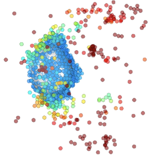
In this work, we consider an initially spherical ‘clump’ of particles suspended in homogeneous isotropic turbulence (see figure 1). Particles are monodisperse with diameters  $d_p=20\ \mathrm {\mu }\textrm {m}$ and particle-to-fluid density ratio $\rho _p/\rho =2200$, corresponding to typical Geldart A/C-type particles (e.g. dust or powder in air) in which inter-particle cohesion is important (McCave Reference McCave1984; Wang, Zhu & Beeckmans Reference Wang, Zhu and Beeckmans2000). The simulation domain is triply periodic with sides of length $L=400 d_p$. The initial aggregate is formed by randomly distributing particles throughout the domain and assigning inward-facing normal velocities, commonly referred to as the ‘centripetal packing method’ (Liu, Zhang & Yu Reference Liu, Zhang and Yu1999; Yang et al. Reference Yang, Wu and Adams2015; Ruan et al. Reference Ruan, Chen and Li2020). First, particles are initially randomly distributed within in a spherical region without overlap. A constant centripetal force is then imposed on each particle to attract the particles towards the center of the domain. Particles undergo collisions and agglomerate in the absence of fluid forces until a single aggregate is formed. The aggregate is then submerged in the flow and held in place until a statistical stationary state is reached. At $t=0$ the particles are free to evolve, potentially resulting in breakup and the formation of smaller aggregates, sometimes referred to as ‘flocs’ in liquid suspensions (Pandya & Spielman Reference Pandya and Spielman1983; Flesch, Spicer & Pratsinis Reference Flesch, Spicer and Pratsinis1999; Jarvis et al. Reference Jarvis, Jefferson, Gregory and Parsons2005; Vowinckel et al. Reference Vowinckel, Biegert, Luzzatto-Fegiz and Meiburg2019a; Zhao et al. Reference Zhao, Vowinckel, Hsu, Köllner, Bai and Meiburg2020).
Simulation configuration shown with background fluid velocity (blue, low; red, high). Particles are initially close-packed in a spherical aggregate of diameter  $D$. Particles are fixed in place until the flow reach a statistically stationary state prior to deagglomeration.

The competition between turbulent shear stress and inter-particle cohesion on the breakup process is studied by adjusting the initial aggregate diameter  $D$, the Hamaker constant $A$ and Taylor Reynolds number ${Re}_\lambda =u_{rms}\lambda /\nu$ where $\nu$ is the kinematic viscosity, $u_{rms}$ is the average root-mean-square velocity and $\lambda = \sqrt {15 \nu /\epsilon }u_{rms}$ is the Taylor microscale with $\epsilon$ the viscous dissipation rate. The particle adhesion number is introduced to quantify the effect of van der Waals attraction, defined as ${Ad} = 2\gamma / ( \rho _p u_{rms}^2 d_p )$ where $\gamma = A/(24{\rm \pi} \delta ^2)$ is the potential energy associated with van der Waals force with $\delta = 0.165$ nm (Marshall & Li Reference Marshall and Li2014). The Hamaker constant $A$ is a material property that indicates the strength of cohesion due to van der Waals (Hamaker Reference Hamaker1937). In this study, $A$ is varied between $\mathcal {O}(10^{-21})$ J for weakly cohesive particles (e.g. silica) and $\mathcal {O}(10^{-18})$ J for strongly cohesive materials such as metal oxides (Marshall & Li Reference Marshall and Li2014). A list of relevant two-phase flow parameters used in each case is provided in table 1.
Parameters used in the simulations with square brackets denoting the parameter range.

2.2. Gas-phase equations
Despite the relatively small size of the particles ( $d_p<\eta$), two-way coupling between the phases must be taken into account because particles are initially close-packed within an aggregate of size $D>\eta$. To account for the presence of particles without requiring a resolution sufficient to resolve the boundary layers at the surface of each particle, a volume filter is applied to the constant-density Navier–Stokes equations (Anderson & Jackson Reference Anderson and Jackson1967), thereby replacing the point variables (fluid velocity, pressure, etc.) by smoother, locally filtered fields. The volume-filtered conservation equations for a constant-density fluid are given by
 \begin{equation} \frac{\partial \alpha}{\partial t}+\boldsymbol{\nabla} \boldsymbol{\cdot}(\alpha \boldsymbol{u})=0, \end{equation}
and
 \begin{equation} \frac{\partial \alpha \boldsymbol{u}}{\partial t}+\boldsymbol{\nabla} \boldsymbol{\cdot}(\alpha \boldsymbol{u} \otimes \boldsymbol{u})=\boldsymbol{\nabla} \boldsymbol{\cdot} \boldsymbol{\tau}+\boldsymbol{F}_{{inter}}+\boldsymbol{F}_{t}, \end{equation}
where  $\boldsymbol {u}$ is the fluid velocity, $\alpha$ is the fluid volume fraction and $\boldsymbol {\tau }=-p/\rho \boldsymbol {I}+\nu (\boldsymbol {\nabla } \boldsymbol {u}+\boldsymbol {\nabla } \boldsymbol {u}^{\top }-\frac {2}{3}(\boldsymbol {\nabla } \boldsymbol {\cdot } \boldsymbol {u}) \boldsymbol {I})$ is the stress tensor with $p$ the fluid-phase pressure and $\boldsymbol {I}$ the identity matrix. Here $\boldsymbol {F}_{{inter}}$ is the interphase exchange term owing to particles that is defined in § 2.4 and $\boldsymbol {F}_{t}$ is a linear forcing term to enforce statistically stationary turbulence. It is important to note that most standard forcing techniques are not sufficient at maintaining desired turbulence properties (e.g. ${Re}_\lambda$) when two-way coupling is present (Mallouppas, George & van Wachem Reference Mallouppas, George and van Wachem2013). In this work, we propose to extend the linear forcing scheme of Lundgren (Reference Lundgren2003), such that the mean interphase exchange contribution is removed and the turbulence statistics remain unaffected by the presence of particles, given by
 \begin{equation} \boldsymbol{F}_{t} = Q_{t} \left( \alpha \boldsymbol{u} - \langle \alpha \boldsymbol{u} \rangle \right)- \langle \boldsymbol{F}_{{inter}} \rangle, \end{equation}
where  $Q_{t}$ is the linear forcing coefficient, and $\langle \cdot \rangle$ denotes the volumetric mean of the quantity within the computational domain.
The equations are implemented in the framework of NGA (Desjardins et al. Reference Desjardins, Blanquart, Balarac and Pitsch2008), a fully conservative solver tailored for turbulent flow computations. The Navier–Stokes equations are solved on a staggered grid with second-order spatial accuracy for both the convective and viscous terms, and the second-order accurate semi-implicit Crank–Nicolson scheme of Pierce (Reference Pierce2001) is used for time advancement.
2.3. Particle-phase equations
Particles are treated in a Lagrangian manner where the translational and rotational motion of an individual particle  $i$ is given by
 \begin{gather} \frac{\textrm{d} \kern0.06em \boldsymbol{x}_p^{(i)}}{\textrm{d}t} = \boldsymbol{v}_p^{(i)}, \end{gather}
 \begin{gather}m_p\frac{\textrm{d}\boldsymbol{v}_p^{(i)}}{\textrm{d}t}={\boldsymbol{f}}_{{inter}}^{(i)}+\boldsymbol{f}_{{col}}^{(i)}+ \boldsymbol{f}_{vw}^{(i)}, \end{gather}
and
 \begin{equation} I_p\frac{\textrm{d}\boldsymbol{\omega}_p^{(i)}}{\textrm{d}t}=\sum_{j} \frac{d_p}{2} \boldsymbol{n}_{ij} \times \boldsymbol{f}^{col}_{t,j\rightarrow i}, \end{equation}
where  $\boldsymbol {x}_p^{(i)}$, $\boldsymbol {v}_p^{(i)}$ and $\boldsymbol {\omega }_p^{(i)}$ are the instantaneous particle position, velocity and angular velocity, respectively, $m_p=\rho _p{\rm \pi} d_p^3/6$ is the particle mass, $I_p=m_p d_p^2/10$ is the moment of inertia for a sphere and $\boldsymbol {n}_{ij}$ is the unit normal vector outward from particle $i$ to particle $j$. The translational motion of each particle is determined by momentum exchange with the gas phase, $\boldsymbol {f}_{{inter}}^{(i)}$, which is defined in § 2.4, in addition to inter-particle collisions $\boldsymbol {f}_{{col}}^{(i)}$ and van der Waals attraction $\boldsymbol {f}_{vw}^{(i)}$, which will be made explicit in the following sections. Particle rotation is a consequence of the tangential component of the collision force, $\boldsymbol {f}^{col}_{t,j\rightarrow i}$.
Owing to the large density ratio under consideration ( $\rho _p/\rho =2200$), the effects of fluid torque and lubrication forces on particle motion are neglected. In addition, it is important to note that cohesion due to van der Waals attraction and collisions are treated independently, which implicitly assumes these effects are additive in nature according to the Derjaguin, Muller and Toporov (DMT) theory (Derjaguin, Muller & Toporov Reference Derjaguin, Muller and Toporov1975). The underlying assumption of the DMT theory is that cohesive forces do not modify the surface profile during particle contact. Another popular contact theory proposed by Johnson, Kendall & Roberts (Reference Johnson, Kendall and Roberts1971), known as the Johnson, Kendall and Roberts (JKR) theory, assumes that adhesion occurs only within the flattened contact region such that the collision force is nonlinearly coupled with the cohesion force and consequently cannot be treated as additive. As suggested by Johnson & Greenwood (Reference Johnson and Greenwood1997), the DMT approximation is valid when $\lambda _T \ll 1$ (typically $\lambda _T \lesssim 0.1$) and the JKR model is valid when $\lambda _T \gg 1$ (typically $\lambda _T \gtrsim 10$), with $\lambda _T$ the dimensionless Tabor parameter defined as
 \begin{equation} \lambda_T = \left( \frac{2d_p\gamma^2}{E_s^2\delta^3} \right)^{1/3}, \end{equation}
where  $E_s$ is the elastic modulus of particles. For the simulations considered herein, $0.19\leqslant \lambda _T\leqslant 0.98$, and it is therefore not immediately obvious which assumptions readily apply. To this end, a variance-based sensitivity analysis is performed in appendix A. It is found that the results reported herein are largely unaffected by the choice in contact theory. The results were also found to be insensitive to the restitution coefficient and inclusion of fluid torque. In the remainder of this work, particle contact mechanics are based on the DMT theory owing to the low values of $\lambda _T$ under consideration and to be consistent with a recently proposed cohesion model that enables larger simulation timesteps (Gu, Ozel & Sundaresan Reference Gu, Ozel and Sundaresan2016), which is discussed in § 2.3.2.
2.3.1. Inter-particle collisions
Particle collisions are needed to prevent unphysical overlap that may arise when attractive inter-particle forces are present (Yao & Capecelatro Reference Yao and Capecelatro2018). In this work, normal and tangential collisions are modelled using a soft-sphere approach originally proposed by Cundall & Strack (Reference Cundall and Strack1979). When two particles come into contact, a repulsive force is created as
 \begin{equation} \boldsymbol{f}^{col}_{n,j \rightarrow i}=\left\{ \begin{array}{@{}ll} -k \delta_{ij}\boldsymbol{n}_{ij} -\zeta\boldsymbol{v}_{ij,n} & \textrm{if}\ s < 0,\\ 0 & \textrm{else, } \end{array}\right. \end{equation}
where  $s$ is the distance between the particle surfaces, $\delta _{ij}$ is the overlap between the particles, $\boldsymbol {n}_{ij}$ is the unit normal vector from particle $i$ to particle $j$ and $\boldsymbol {v}_{ij,n}$ is the normal relative velocity between particles $i$ and $j$. The spring stiffness and damping parameter are given by $k$ and $\zeta$, respectively. A model for the damping parameter (Cundall & Strack Reference Cundall and Strack1979) uses a coefficient of restitution $0<\textrm {e}<1$ such that
 \begin{equation} \zeta=-2\ln \textrm{e}\frac{\sqrt{k m_p/2}}{\sqrt{{\rm \pi}^2+\left(\ln \textrm{e}\right)^2}}. \end{equation}
The spring stiffness is related to the collision time,  $\tau _{col}$, according to
 \begin{equation} k=m_p/2\tau_{col}^2\left({\rm \pi}^2+\left(\ln{\textrm{e}}\right)^2\right). \end{equation}
Collisions are treated as inelastic with a coefficient of restitution  $\textrm {e}=0.9$, representative of many solid spherical objects in dry air. To properly resolve the collisions without requiring an excessively small timestep, $\tau _{col}$ is set to be 20 times the simulation time step ${\rm \Delta} t$ for all simulations presented in this work. A detailed account on the sensitivity of the results reported herein to the collision parameters is provided in appendix A.
To account for friction between particles and, thus, particle rotation, the static friction model is employed for the tangential component of the collision force, given by
 \begin{equation} \boldsymbol{f}^{col}_{t,j \rightarrow i}=-\mu_{f}\left| \,\boldsymbol{f}^{col}_{n,j \rightarrow i}\right|\boldsymbol{t}_{ij}, \end{equation}
where  $\mu _f=0.1$ is the coefficient of friction and $\boldsymbol {t}_{ij}$ is the tangential unit vector. Once each individual collision force is computed, the full collision force that particle $i$ experiences can be expressed as
 \begin{equation} \boldsymbol{f}_{col}^{(i)}=\sum_{j{\!\ne}i} \left(\boldsymbol{f}_{n,j\rightarrow i}^{col}+\boldsymbol{f}_{t,j\rightarrow i}^{col}\right). \end{equation}
Further details can be found in Capecelatro & Desjardins (Reference Capecelatro and Desjardins2013).
2.3.2. Van der Waals models compatible with soft-sphere collisions
The magnitude of the van der Waals force between two particles  $i$ and $j$ of the same size, $F_{ij}^{{vw}}$, is modelled as (Hamaker Reference Hamaker1937)
 \begin{equation} F_{i j}^{{vw}}(A, s)=\frac{A}{6} \frac{d_p^2\left(d_p+s\right)}{s^{2}(2d_p+s)^{2}}\left[\frac{s\left(2d_p+s\right)}{(d_p+s)^{2}}-1\right]^{2}. \end{equation}
Owing to the short range nature of the van der Waals force, it is assumed that the force saturates at a minimum separation,  $s_{min} = 1\times 10^{-9}$ m and is cut off at $s_{max} = d_p/4$.
A brute-force implementation of the unmodified Hamaker model would require excessively small time steps to resolve inter-particle contact forces. As described previously, the spring stiffness  $k$ used in the soft-sphere collision model is determined based on the collision time $\tau _{col}$ according to (2.10), resulting in artificially ‘soft’ particles to enable larger time steps. A modified van der Waals model was recently proposed to be compatible with the soft-sphere collision model outlined in § 2.3.1 (Gu et al. Reference Gu, Ozel and Sundaresan2016). The modification ensures the work done by the van der Waals force remains unchanged when particles overlap, such that its overall effect is insensitive to the choice of $k$ and consequently the results remain unchanged as ${\rm \Delta} t$ is adjusted. This is accomplished by modifying the saturation distance and Hamaker constant when two particles are in direct contact, according to
 \begin{equation} \boldsymbol{f}_{vw}^{(i)}=-F_{vw}^{(i)} \boldsymbol{n}_{i j}=\left\{\begin{array}{@{}ll} {-F_{ij}^{vw}(A, {s-s_0}) \boldsymbol{n}_{i j}} & {\text{for} \ s_{min}^s < s < s_{max}}\\ {-F_{ij}^{vw}\left(A^s, s_{min }\right) \boldsymbol{n}_{i j}} & {\text{for}\ s \leqslant s_{min}^s},\end{array}\right. \end{equation}
with  $A^s=A( k/k_r)^{1/2}$ where $k_r$ is the ‘real’ spring stiffness of the particle that would result in negligible overlap during collisions. A value of $k_r = 7000\ \textrm {N}\ \textrm {m}^{-1}$ is used and the simulation spring stiffness $k$ is chosen such that $k_r/k=700$ as described in Gu et al. (Reference Gu, Ozel and Sundaresan2016). The offset $s_0$ and shifted saturation distance $s_{min}^s$ can be obtained by solving the following nonlinear equations
 \begin{equation} F_{vw}\left(\theta, s_{min }^{R}\right)=F_{vw}\left(1, s_{min }^{s}-s_{0}\right), \end{equation}
and
 \begin{align} F_{vw}\left(1, s_{min }\right) \cdot s_{min }+\int_{s_{min }}^{s_{max }} F_{vw}(1, s) \,\textrm{{d}} s=F_{vw}\left(\theta, s_{min }\right) \cdot s_{min}^s +\int_{s_{min}^{s}}^{s_{max}} F_{vw}\left(1, s-s_{0}\right) \textrm{{d}} s. \end{align}
A bisection method is used to solve the nonlinear system of equations as a preprocessing step prior to simulation runtime.
2.4. Two-way coupling
Particle information is projected to the mesh using a Gaussian filtering kernel  $\mathcal {G}$ with a characteristic length $\delta _f$. The local volume fraction and interphase exchange term appearing in the fluid-phase equations (2.1)–(2.3) are evaluated as
 \begin{equation} \alpha=1-\sum_{i=1}^{N_{p}} \mathcal{G}\left(\left|\boldsymbol{x}-\boldsymbol{x}_{p}^{(i)}\right|\right) V_p, \end{equation}
and
 \begin{equation} \boldsymbol{F}_{{inter }}=-\frac{1}{\rho}\sum_{i=1}^{N_{p}} \mathcal{G}\left(\left|\boldsymbol{x}-\boldsymbol{x}_{p}^{(i)}\right|\right) \boldsymbol{f}_{{inter }}, \end{equation}
where  $V_p={\rm \pi} d_p^3/6$ is the particle volume, and the momentum exchange term for particle $i$ is given by
 \begin{equation} \boldsymbol{f}_{{inter}}^{(i)} = \boldsymbol{f}_{{drag}}^{(i)}+\rho V_p \boldsymbol{\nabla} \boldsymbol{\cdot} \boldsymbol{\tau}[ \boldsymbol{x}_p^{(i)} ], \end{equation}
which contains contributions of resolved fluid stresses at the particle location ( $\boldsymbol {\tau }[\boldsymbol {x}_p^{(i)}]$) and unresolved stresses (i.e. drag) modelled according to
 \begin{equation} \frac{{\boldsymbol{f}}_{{drag}}^{(i)}}{m_p}=\frac{F\left(\alpha, {Re}_{p}\right)}{\tau_p} \alpha \left(\boldsymbol{u}[\boldsymbol{x}_p^{(i)}]-\boldsymbol{v}_p^{(i)}\right), \end{equation}
where  $\boldsymbol {u}[\boldsymbol {x}_p^{(i)}]$ is the fluid velocity at the location of particle $i$,
$i$,  ${Re}_p =\alpha \| \boldsymbol {u}[\boldsymbol {x}_p^{(i)}]-\boldsymbol {v}_p^{(i)}\| d_p/\nu$ is the particle Reynolds number and $\tau _p = \rho _pd_p^2/(18\rho \nu )$ is the particle response time. In this work, $F(\alpha , {Re}_{p})$ is modelled according to the dimensionless drag coefficient of Tenneti, Garg & Subramaniam (Reference Tenneti, Garg and Subramaniam2011) to take into account finite Reynolds number and volume fraction effects on the drag force.
In order to project the particle data to the grid in an efficient manner and ensure numerical stability, the two-step filtering approach of Capecelatro & Desjardins (Reference Capecelatro and Desjardins2013) is employed. First the particle data is sent to the neighbouring grid points via trilinear extrapolation, the solution is then diffused such that the projection resembles a Gaussian with characteristic size of  $\delta _f$. To avoid restrictive time step constraints in the diffusion process, the latter step is solved implicitly via approximate factorization with a second-order alternating direction implicit (ADI) scheme. In this work, the filter size $\delta _f=8d_p$. Such an approach has been demonstrated to accurately predict the characteristics of particle clustering in turbulent flows (Capecelatro, Pepiot & Desjardins Reference Capecelatro, Pepiot and Desjardins2014). This simulation framework was recently demonstrated to provide accurate results when considering attractive inter-particle forces due to electrostatics (Yao & Capecelatro Reference Yao and Capecelatro2018, Reference Yao and Capecelatro2019).
2.5. Numerical time-stepping
The wide range of time scales associated with cohesive particles in turbulent flows presents a significant challenge in numerical simulations. In the present work, the fluid time scale  $\tau _f=(\nu /\epsilon )^{1/2}$ is $\mathcal {O}(10^{-3}\ \textrm {s})$, whereas the particle response time $\tau _p=\mathcal {O}(10^{-5}\ \textrm {s})$ and the collision time scale $\tau _{col}=\mathcal {O}(10^{-7}\ \textrm {s})$, even with the artificially softened particles and modified van der Waals model. In order to properly resolve the time scales at play in a tractable manner, a multiscale time-stepping framework based on the method proposed by Marshall (Reference Marshall2009) is employed (see figure 2). In this approach, the fluid equations are solved on a separate time scale from the particles. To avoid $\mathcal {O}(N_p^2)$ calculations of the inter-particle forces, a nearest-neighbour detection algorithm is employed, such that interactions via collisions and van der Waals are only considered between particles in adjacent grid cells (Capecelatro & Desjardins Reference Capecelatro and Desjardins2013). The fluid time step, ${\rm \Delta} t$, is limited by the convective time scale dictated by the Courant–Friedrichs–Lewy (CFL) number. To simplify the implementation of the two-way coupling described in § 2.4, the fluid time step is further constrained to prevent particles from moving more than one grid cell, i.e. ${\rm \Delta} t<{\rm \Delta} x/\max {|\boldsymbol {v}_p|}$. This ensures that the particle nearest-neighbour list only needs to be updated once per fluid time step. The particle advection time scale, $\tau _{adv}=d_p/|\boldsymbol {v}_p|$, must be small enough to prevent significant overlap between particles. To ensure the particle dynamics are well resolved, particles are subiterated each fluid time step based on a time scale that is one order of magnitude smaller than the minimum of the collision time, particle response time and particle advection time. Finally, a second-order Runge–Kutta scheme is used for updating each particle's position, velocity and angular velocity.
Multiscale time-stepping algorithm used in the simulations. For each fluid time step  ${\rm \Delta} t$, particles are subiterated at a smaller time step ${\rm \Delta} t_p$ until they are in sync with the fluid.

3. Results and discussion
3.1. Flow visualization
Simulations are carried out for three Taylor microscale Reynolds numbers and five adhesion numbers as listed in table 1. The spatial distribution of particles at  $t/\tau _p = 4$ is compared in figure 3. In the absence of van der Waals forces, the aggregate breaks up immediately and particles are dispersed by the background turbulence. It can be observed that particles progressively shed off from the surface of the clump, and gain speed as they are transported away. Particles within the aggregate experience smaller interphase slip velocities owing to two-way coupling, resulting in negligible drag forces. It is important to note that the deagglomeration process would be markedly different if two-way coupling were not taken into account. If the simulation was performed with one-way coupling, all of the particles would experience similar drag, resulting in simultaneous breakup throughout the aggregate (see appendix A).
The first column shows an initially spherical particle aggregate ( $D=20d_p$) suspended in homogeneous isotropic turbulence. The remaining columns show particle positions after $t/\tau _p = 4$ coloured by their velocity (blue, low; red, high) for different values of ${Ad}$ and ${{Re}_\lambda }$.

As  ${Ad}$ increases, inter-particle cohesion eventually overcomes the fluid stresses, preventing breakup from occurring when ${Ad}\geqslant 9$. For the same ${Ad}$, the rate of deagglomeration increases with increasing ${Re}_\lambda$ due to larger fluid velocity fluctuations. It is clear from figure 3 that the competition between turbulent stresses acting to disintegrate the particle aggregate and cohesive forces opposing breakup is entirely controlled by ${ Re}_\lambda$ and ${Ad}$. A quantitative assessment of ${ Re}_\lambda$ and ${Ad}$ on the evolution of the breakup process is presented in the following sections.
3.2. The role of turbulence intermittency on deagglomeration
Fluid stresses exerted on the aggregate surface by turbulence is highly intermittent. Figure 4 shows a comparison of the fluid stress at the aggregate surface, defined as  $\rho u'^2 \vert _{c} = \sum _{i=1}^{N_p} \rho \lVert \boldsymbol {u}'[\boldsymbol {x}_p^{(i)}] \rVert ^2/N_p$, with the domain-averaged stress. As can be seen, the instantaneous fluid stress at the vicinity of the aggregate fluctuates by as much as four times the domain-averaged value. The time scales of these fluctuations are significantly smaller than the time required to complete breakup ( ${\sim }300\tau _f$ for this case), which amplifies the effect of turbulence intermittency on early stage breakup.
Instantaneous fluid stress at the aggregate surface ( $-$) and within the entire domain ( $--$) normalized by the root-mean-square quantities with ${Re}_\lambda = 30$ and ${Ad} = 0.3$. Four realizations under consideration ( ${\bullet }$, red).

To investigate the effect of turbulence intermittency on the breakup process, particles are held in place until four values of  $t/\tau _f$ as highlighted in red in figure 4. The particle clump is then free to evolve from that particular instant in time. These four realizations contain different fluid stress levels at the vicinity of the clump. In order to quantify its effect on breakup, the gyration radius, $R_g$, and the fractal dimension, $D_f$, are computed, which are commonly used to characterize the dynamics and morphology of particle aggregates (Friedlander Reference Friedlander2000; Ruan et al. Reference Ruan, Chen and Li2020). The gyration radius is defined as
 \begin{equation} R_{g}=\sqrt{\frac{1}{N_c} \sum_{i=1}^{N_c}\left\Vert \boldsymbol{x}_{p}^{(i)}-\boldsymbol{x}_{c} \right\Vert^{2}}, \end{equation}
where  $N_c$ is the number of particles in the clump, $\boldsymbol {x}_c = \sum _{i=1}^{N_c} \boldsymbol {x}_p^{(i)} / N_c$ is the center of mass of the aggregate. The fractal dimension indicates the compactness of its spatial structure. For a dense spherical aggregate, $D_f \approx 3$. In this work, we follow Ruan et al. (Reference Ruan, Chen and Li2020) and obtain $D_f$ by solving the following nonlinear equation
 \begin{equation} N_c = k_f \left( 2R_g/d_p\right)^{D_f}, \end{equation}
where the fractal prefactor  $k_f$ is
 \begin{equation} k_f = 0.7321 + 0.8612^{( ({D_f-1})/{2})^{1.95}}. \end{equation}
The initial clump generated by centripetal packing has values  $R_g/d_p = 7.625$ and $D_f = 2.94$. The total volume of the clump is defined by $V_c(t)=\{\boldsymbol {x}\in \mathbb {R}^3:\alpha (\boldsymbol {x},t)<0.75\}$, which is evaluated at each simulation timestep in order to quantify the evolution of $R_g$ and $D_f$. $N_c$ represents the number of particle inside the volume $V_c(t)$.
Figure 5 shows the temporal evolution of  $N_c$, $R_g$ and $D_f$ for the four realizations with ${Re}_\lambda = 64$ and ${Ad = 0.3}$. It can be seen that the breakup statistics change substantially over the different realizations despite ${Re}_\lambda$ and ${Ad}$ being held constant. The cases with higher initial turbulence intensity result in quicker initial breakup yet later time statistics remain relatively unchanged. This can be associated with the time scale of the intermittent fluctuations being significantly smaller than the time it takes for total breakage. Although the aggregate breaks up faster with larger initial surface stress, it is subject to smaller fluctuations on average (see figure 4) resulting in slower breakage at late times. Despite this intermittency, $N_c$ decays in an approximately linear manner whereas $R_g$ decreases much faster at late time. The fractal dimension $D_f$ decreases from $2.94$ to approximately $2.5$, indicating significant deformation of the aggregate. Note that the statistics of the fractal dimension $D_f$ becomes noisy when the number of particles in the aggregate is $N_c \lessapprox 1000$ or equivalently the gyration radius $R_g \lessapprox 2d_p$ owing to the limited sample size. To mitigate the effect of turbulence intermittency on the subsequent results reported herein, all simulations are initialized such that $\rho u'^2 \vert _{c}$ is approximately equal to the global fluid stress at $t=0$.
Characteristics of the aggregate for four different realizations with  ${Re}_\lambda = 64$ and ${Ad = 0.3}$: (a) number of particles, (b) normalized Gyration radius and (c) fractal dimension of the particle clump. Line types $-$,
$-$,  $-\,\cdot$, $--$ and $\cdots$ correspond to red data points from left to right shown in figure 4.

3.3. Early stage deagglomeration
Figure 6 shows the temporal evolution of the number of particles  $N_c$ and the gyration radius $R_g$ of the aggregate for ${Re}_\lambda = 64$ as a function of ${Ad}$. The number of particles within the aggregate decreases linearly as it breaks up. As ${Ad}$ increases, inter-particle cohesive forces become more significant, resulting in a decreased rate of deagglomeration. It can be seen that the deagglomeration statistics exhibit a stair-step behaviour when ${Ad}$ exceeds a critical value of ${Ad} = 3$. This is attributed to the intermittency of turbulent fluctuations, as shown in figure 7. Particles shed off from the aggregate more rapidly when the clump experiences larger velocity fluctuations. Similar trends are also observed for the gyration radius, whereas the radius decreases faster during the late stage of deagglomeration, as a direct consequence of the linear decay in $N_c$, or equivalently linear decay in aggregate volume. Note that when ${Ad}>3$, particles become so cohesive that the clump retains its original shape and size, which were omitted from figure 6.
Temporal evolution of (a) the number of particles and (b) gyration radius of the aggregate for  ${Re}_\lambda = 64$ and ${Ad} = 0,0.3,0.6,1.2,1.8,3$ (from black to light gray).

The plots on the left temporal evolution of the number of particles (blue) and gyration radius (red) of the aggregate and corresponding fluid stress at the aggregate surface for  ${Ad} = 3$ and ${Re}_\lambda = 64$. Stair-step behaviour is observed in the statistics indicating intermediate breakup occurs when the local fluid stress exceeds a threshold value. In ( $a$)–( $f$) the corresponding instantaneous snapshots of particle position are shown, with iso-contour of $\alpha = 0.75$ (white) representing the surface of the aggregate. Colour scheme is the same as figure 3.

Figure 7 highlights the effect of fluid stresses at the aggregate surface for  ${Ad}=3$ and ${Re}_\lambda = 64$. The iso-contour of $\alpha = 0.75$ shown in white is used to visualize the surface of the aggregate. A direct one-to-one correspondence can be observed between the stair-step breakup behaviour and instantaneous turbulent velocity fluctuations. The snapshots indicate the abrupt decrease in aggregate size is associated with turbulent eddies interacting with the aggregate resulting in breakup of smaller satellite aggregates. Before breakage, the clump is seen to remain relatively spherical. In the presence of large velocity fluctuations, the aggregate breaks from the side of its surface where the velocity gradient is high. As the aggregate shrinks, the net effect of cohesion within the aggregate also decreases and consequently breaks up in all directions. Although the surface area is smaller than the original aggregate, particles shed off at higher speeds resulting in the same rate-of-change in $N_c$. At late time ( $t>1000\tau _f$), $D$ drops below a critical value where turbulent eddies can no longer break the aggregate into smaller pieces, i.e. when $D\sim \eta$.
3.4. Scaling analysis
To better understand the role of turbulence and adhesion on the breakup process, the breakage outcome associated with each simulation is plotted in terms of the adhesive stress,  $\gamma /\eta$, and the turbulent stress, $\rho _p u_{rms}^2$. As shown in figure 8, larger fluid stress results in a transition from a ‘no breakage’ regime to a ‘breakage’ regime at a given $\gamma /\eta$. A simulation is classified as ‘no breakage’ when $N_c$ remains unchanged for $t \geqslant 1000\,\tau _f$. Similarly, at a given $\rho _p u_{rms}^2$, the increase of $\gamma /\eta$, either due to enhanced cohesion or smaller $\eta$, reduces the likelihood of breakup. The breakup outcome is found to depend on a turbulent adhesion number ${Ad}_{\eta , {crit}}=\gamma /(\rho _{p} u_{{rms}}^{2} \eta )=1.8$ where ${Ad}_{\eta } = {Ad}(d_p/\eta )$. Note that for simple shear flow where $\eta$ is not well defined, it has been found that the breakage outcome is instead characterized by $D$ (Ruan et al. Reference Ruan, Chen and Li2020). The simulations performed in the present study indicate that the characteristic length scale associated with aggregate breakup is $\eta$ when $\eta \ll D$. In simple shear flow, particles experience a uniform shear rate within the aggregate, therefore larger aggregates will experience larger velocity differences across the surface. In homogeneous isotropic turbulence, however, turbulent eddies create local regions of high shear of size proportional to $\eta$. When $\eta \ll D$, these eddies are agnostic to the clump size $D$ resulting in progressive breakup into smaller clumps, as depicted in figure 7.
Breakage regime diagram for a particle aggregate suspended in homogeneous isotropic turbulence for  ${Re}_\lambda = 30$ ( $\blacklozenge$, red), 43 ( $\bullet$, green), 64 ( $\blacktriangle$, blue) and non-dimensional clump size $D/d_p = 10\ \text {(solid)}, 20\ \text {(hollow)}$, with $+$ and $\times$ denoting cases without breakage for $D/d_p = 10$ and 20, respectively. The linear dashed line separating the breakup outcome is given by ${Ad}_{\eta , {crit}}=\gamma /(\rho _{p} u_{{rms}}^{2} \eta )=1.8$.

Figure 6 shows that the breakup rates ( ${\dot{N}_c} = \textrm {d}N_c/\textrm {d}t$) are approximately constant for each case under consideration. The breakup rates are extracted from each simulation and plotted in figure 9(a). It can immediately be seen that the breakup rate increases with $D$ and ${Re}_\lambda$, but decreases with ${Ad}$. The effect of $D$ and ${Re}_\lambda$ can be taken into account via an aggregate Reynolds number ${Re}_D = u_{rms} D / \nu$. When ${Ad}_\eta =0$, adhesion has no effect on the breakup rate and consequently ${\dot{N}_c}\tau _p \sim {Re}_D$. When ${Ad}_\eta \geqslant {Ad}_{\eta ,{crit}}$, no breakage will occur according to figure 8 ( ${\dot{N}_c}\tau _p=0$). With this, a correction factor $(1 - {Ad}_\eta /{Ad}_{\eta ,{crit}})$ can be introduced to account for the effect of cohesion. Based on these observations, the data is rescaled with respect to ${Re}_D(1 - {Ad}_\eta /{Ad}_{\eta ,{crit}})$. As shown in figure 9(b), the breakup rate follows a linear scaling given by ${\dot{N}_c}\tau _p=28\,{Re}_D(1 - {Ad}_\eta /{Ad}_{\eta ,{crit}})$. Note that small deviations are observed at lower Reynolds numbers (e.g. ${Re}_\lambda =30$). For these cases, the eddy size becomes comparable to $D$, and turbulence must break up the entire aggregate instead of a piece of it. As a result, the assumption that $\eta$ is the characteristic length scale for deagglomeraton does not hold at low Reynolds numbers and the breakup will exhibit dependance of $D/d_p$ instead. Based on the simulation results, the dependence of breakup on $\eta$ is applicable when $D/\eta \gtrsim 5$.
Rate of deagglomeration quantified by the time-rate-of-change of number of particles within the aggregate for different  ${Ad}$, ${Re}_\lambda = 30$ ( $\blacklozenge$, red), 43 ( $\bullet$, green), 64 ( $\blacktriangle$, blue) and aggregate size $D/d_p = 10\ \text {(solid)}, 20\ \text {(hollow)}$. Rate of deagglomeration plotted (a) as a function of Ad and (b) as a function of ${Re}_D(1 - {Ad}_\eta /{Ad}_{\eta ,{crit}})$. Here ${\dot{N}_c}\tau _p=28\,{Re}_D(1 - {Ad}_\eta /{Ad}_{\eta ,{crit}})$ ( $--$).

4. Phenomenological model of deagglomeration
Despite valuable insights provided by the numerical simulations presented herein and many other works using PR-DNS, they are limited to relatively small-scale systems owing to the high computational cost needed to resolve the relevant length and time scales. Particle transport in large-scale systems is typically modelled without knowledge of the velocity field at the scale of individual particles. However, the breakup of cohesive particles reported in §§ 3.2 and 3.3 are shown to depend strongly on local turbulence statistics such as  $\eta$ and $u_{rms}$. In addition, the effect of turbulence intermittency is not captured when particles traverse an averaged flow field, such as in the case of RANS. The aim here is to develop a reduced-order model capable of capturing the breakup of cohesive particles in the absence of a resolved turbulent flow field.
The Taylor analogy breakup (TAB) model is widely used in calculating droplet breakup. This method is based on Taylor's analogy (Taylor Reference Taylor1963) for an oscillating and distorting droplet. The droplet deformation is treated as a mass–spring–damper system, where the surface tension force acts as a restorative force, the force exerted by the surrounding gas phase acts as an external force, and the droplet viscosity acts as a damper. Motivated by the TAB model, we propose a similar mass–spring–damper analogy to model turbulence-induced breakup of cohesive particles. In this case, the van der Waals force is treated as an analogue to the droplet surface tension, and friction due to inter-particle contact is treated as an analogue to the droplet viscosity. We refer to this model as a granular Taylor analogy breakup (G-TAB) model.
Assuming the local turbulence statistics are known from a turbulence model such as RANS,  ${Ad}_\eta$ can be determined to estimate whether or not breakup occurs. As shown in figure 10, three distinct breakup regimes are observed: ${Ad}_\eta \leqslant 0.5$, the cohesive force is weak compared with turbulent stresses and the aggregate breaks up instantaneously; $0.5<{Ad}_\eta \leqslant 1.8$, the competition between turbulence and cohesion results in delayed breakage of the aggregate; and when cohesion becomes significant ( ${Ad}_\eta >1.8$), turbulence is unable to overcome the attractive forces, resulting in no breakup. The G-TAB model is employed to predict the breakup time as a function of ${Ad}_\eta$ when $0.5<{Ad}_\eta \leqslant 1.8$. The governing equation is given by
 \begin{equation} F-k x-d \frac{\textrm{d}\kern0.06em x}{\textrm{d} t}=m \frac{\textrm{d}^{2} x}{\textrm{d} t^{2}}, \end{equation}
where  $x$ is the displacement of the aggregate equator from its spherical (undisturbed) position. The coefficients of this equation are based on Taylor's analogy, given as
 \begin{gather} \text{inertial force due to turbulence: }\quad \frac{F}{m} = C_{F} \frac{\rho u_{rms}^{2}}{\rho_{p} \eta}, \end{gather}
 \begin{gather}\text{restorative force due to adhesion: }\quad \frac{k}{m} =C_{k} \frac{\gamma}{\rho_{p} \eta^{3}}, \end{gather}
 \begin{gather}\text{damper due to inter-particle friction: }\quad \frac{d}{m} =C_{d} \frac{\mu_{p}}{\rho_{p} \eta^{2}}, \end{gather}
where  $\mu _p$ is the effective solids viscosity at random close packing (RCP) and $C_F$, $C_k$ and $C_d$ are model coefficients that will be determined later.
Time to initial breakup  $t_{br}$ as a function of the turbulent adhesion number. Symbols are the same as figure 8. The black line corresponds to (4.14) with $C_F = 0.8$, $C_k = 2\times 10^{-4}$, $C_d = 0.3$ and $C_b = 1$. The vertical dashed lines correspond to ${Ad}_\eta = 0.5$ and ${Ad}_\eta = 1.8$.

For non-cohesive particles, Bocquet et al. (Reference Bocquet, Losert, Schalk, Lubensky and Gollub2001) gives the solids viscosity as  $\mu _p^{0} = (m_p\sqrt {\varTheta }/d_p^2) g_0^{\beta -1}$ from kinetic theory, where $\varTheta = \langle \boldsymbol {v}_p^{(i)}\cdot \boldsymbol {v}_p^{(i)} \rangle /3$ is the granular temperature, $g_0 = (1-n/n_c)^{-1}$ is the radial distribution function at contact with $n$ the local number density and $n_c$ the maximum number density at RCP. Here $\beta = 1.75$ is a phenomenological constant measured from experiments. For cohesive particles, $\mu _p$ increases monotonically with increasing adhesion due to enhanced inter-particle attraction. A linear correction has been introduced by Roy, Luding & Weinhart (Reference Roy, Luding and Weinhart2017) as $\mu _p = \mu _p^{0} (1+1.47\,{Bo})$ where ${Bo}=F_{vdw}/(p_s d_p^2)$ is the Bond number that measures the cohesion strength relative to the compressive force. The solids pressure $p_s$ at RCP is given as $p_s=n_0g_0m_p\varTheta$ with $n_0 = (1+\textrm {e})({\rm \pi} /3) n_c^2 d_p^3$ (Bocquet et al. Reference Bocquet, Losert, Schalk, Lubensky and Gollub2001). Based on these relations, $\mu _p$ is computed as a function of $\varTheta$ and ${Bo}$
 \begin{equation} \mu_p = (m_p\sqrt{\varTheta}/d_p^2) g_0^{\beta-1} (1+1.47\,{Bo}), \end{equation}
which depends on  ${Re}_\lambda$ and ${Ad}$. Based on the simulation results reported herein, $\varTheta /(\varGamma d_p)^2$ is found to scale linearly with ${{Re}}_D^{-1}$ (see figure 11). Therefore, we propose a simple model for the granular temperature of the particles within the aggregate near RCP as
 \begin{equation} \varTheta = C_{\varTheta} {Re}_D^{-1} (\varGamma d_p)^2, \end{equation}
where the coefficient  $C_{\varTheta }=0.2$ is determined from the simulations, and the shear rate is approximated as $\varGamma \approx u_{rms}/D$. A more detailed algebraic expression for $\varTheta$ was presented by Syamlal, Rogers & O'Brien (Reference Syamlal, Rogers and O'Brien1993).
Scaling of the mean granular temperature within the aggregate for  $D=10d_p$ (blue) and $20d_p$ (red). Here $\varTheta /(\varGamma d_p)^2 = 0.2\,{{Re}}_D^{-1}$ ( $--$).

The aggregate is assumed to break up if the distortion grows to a critical ratio of the Kolmogorov length scale. This breakup requirement is given as
 \begin{equation} y=x /\left(C_{b} \eta\right)>1. \end{equation}
Consequently, (4.2) can be non-dimensionalized as
 \begin{equation} \frac{\textrm{d}^{2} y}{\textrm{d} t^{2}}=\frac{C_{F}}{C_{b}} \frac{\rho}{\rho_{p}} \frac{u_{rms}^{2}}{\eta^{2}}-\frac{C_{k} \gamma}{\rho_{p} \eta^{3}} y-\frac{C_{d} \mu_{p}}{\rho_{p} \eta^{2}} \frac{\textrm{d} y}{\textrm{d} t}, \end{equation}
which exhibits the following analytical solution
 \begin{equation} y(t)={Ad}_{c}\left(1-\textrm{e}^{-\left(t / t_{d}\right)}\left[\cos (\omega t)+\frac{1}{\omega t_d}\sin (\omega t)\right]\right), \end{equation}
where
 \begin{gather} \frac{1}{t_{d}}=\frac{C_{d}}{2} \frac{\mu_{p}}{\rho_{p} \eta^{2}}, \end{gather}
 \begin{gather}{Ad}_{c} = \frac{C_F}{C_k C_b} \frac{1}{Ad_\eta} \frac{\rho_f}{\rho_p}, \end{gather}
and
 \begin{equation} \omega^{2} = C_{k} \frac{\gamma}{\rho_{p} \eta^{3}}-\frac{1}{t_{d}^{2}}. \end{equation}
The aggregate is assumed to break up when the maximum displacement satisfies
 \begin{equation} \max(y) = {Ad}_c \left( \textrm{e}^{-{\rm \pi}/(\omega t_d)}+1 \right) > 1, \end{equation}
and the corresponding breakup time is uniquely obtained by solving
 \begin{equation} y(t_{br}) = 1, \quad t_{br} < {\rm \pi}/\omega. \end{equation}
 The model coefficients are determined by solving (4.10)–(4.12) and (4.14) using  $t_{br}$ extracted from each simulation. The G-TAB model is able to predict $t_{br}$ and the correct ${Ad}_{\eta ,{crit}}$ as shown in figure 10 with $C_F = 0.8$, $C_k = 2\times 10^{-4}$, $C_d = 0.3$ and $C_b = 1$. These coefficients are of the same order as the original TAB model except for $C_k$, which is significantly smaller, indicative that a larger restorative force is required to prevent breakup compared with that of the surface tension required for liquid droplets. This discrepancy is primarily due to the short-range nature of the van der Waals force which results in non-restorative deformation as inter-particle distances increase beyond the force range. Note that the model is not applied when ${Ad}_\eta <0.5$, resulting in the instantaneous breakage regime where $t_{br} = 0$.
In summary, for any spherical aggregate of particles with known size ratio  $D/d_p$, Hamaker constant $A$ and local turbulence quantities $\eta$ and $u_{rms}$, the non-dimensional numbers ${Ad}_\eta$, ${Bo}$ and ${Re}_D$ can be calculated. With this, the G-TAB model predicts the time it takes to initiate breakage based on ${Ad}_\eta$ and ${Bo}$. If an aggregate is predicted to break (i.e. ${Ad}_\eta <1.8$), then the rate of breakup is modelled using the scaling shown in figure 9 given by
 \begin{equation} \mathrm{d}N_c / \mathrm{d} t=\frac{28\,{Re}_D}{\tau_p}(1 - {Ad}_\eta/{Ad}_{\eta,{crit}}). \end{equation}
This provides a comprehensive prediction of the deagglomeration process of a clump of cohesive particles in turbulence from the onset of breakage to complete fragmentation into primary particles. Because  $u_{rms}$ and $\eta$ are readily available in a RANS calculation, the G-TAB model can readily be incorporated. We note that this model is specifically designed for the breakup of a single dense spherical aggregate in turbulence. Although non-spherical or less-densely packed aggregates may require different model coefficients, the mass–spring–damper analogy proposed here is anticipated to hold.
Many efforts have recently been made towards modelling aggregate breakup due to particle interactions. Chen & Li (Reference Chen and Li2020) showed that the collision-induced breakage rate scales exponentially with  ${Ad}$ and aggregate size. van Wachem et al. (Reference van Wachem, Thalberg, Nguyen, de Juan, Remmelgas and Niklasson- Bjorn2020) proposed a discrete fragmentation model (DFM) to simulate the breakup behaviour due to aggregate–aggregate and aggregate–wall collisions without tracking each individual primary particle. Unlike these studies, the present work provides a framework that isolates the effect of turbulence on particle breakup using a simple phenomenological model. At present, experimental measurements of particle breakup in turbulence are scarce. While such measurements are challenging to make experimentally, primarily due to the difficulty in seeding an individual aggregate in a controlled manner and due to the opaque nature of the particles, such data would be invaluable to further validate such models.
5. Conclusion
In the present study, a ‘clump’ of Geldart A/C-type particles (e.g. dust or powder in air) was placed in homogeneous isotropic turbulence to study the interplay between turbulence and adhesion on deagglomeration. Numerical simulations were carried out in an Eulerian–Lagrangian framework that resolves particle–particle interactions and models fluid–particle coupling. The adhesion number  ${Ad}$, Taylor microscale Reynolds number ${Re}_\lambda$ and non-dimensional clump size $D/d_p$ were varied to investigate the breakup criteria and breakup rate of the aggregate.
To fully resolve the wide range of length and time scales present in the system, we employed a multiscale time-stepping algorithm that subiterates particles at a smaller time step than the fluid phase. A modified linear-forcing technique was introduced to maintain statistically stationary turbulence in the presence of particles with two-way coupling. A modified van der Waals model developed for soft-sphere collisions was also adopted to allow for larger simulation time steps while keeping the results insensitive to the choice of particle stiffness. A variance-based sensitivity analysis was performed to quantify the relative importance of the modelling parameters appearing in the particle-phase equations on the time-to-breakup and breakup rate. The simulation results were found to be most sensitive when switching between one-way and two-way coupling. In the absence of two-way coupling, the local flow remains unmodified in the presence of particles, resulting in relatively large interphase slip velocities and consequently instantaneous breakup.
The temporal evolution of the aggregate size and flow visualizations demonstrated that turbulence intermittency plays an important role on the deagglomeration process. It was found that the time rate of breakup is affected substantially by different flow realizations of the same  ${Re}_\lambda$. As particles become more cohesive (e.g. ${Ad} \geqslant 3$), a stair-step behaviour was observed for the breakup rate owing to the presence of large turbulent velocity fluctuations at the vicinity of the aggregate.
The aggregate is shown to breakup progressively into smaller clumps proportional to  $\eta$. A regime map of fluid stress versus adhesive stress revealed that a critical turbulent adhesion number, ${Ad}_{\eta , {crit}}=\gamma /(\rho _{p} u_{{rms}}^{2} \eta )=1.8$, is capable of predicting the breakup outcome of an aggregate in turbulence. A scaling analysis further demonstrated a linear relation between the time rate of breakup ${\dot{N}_c}$ and the aggregate Reynolds number ${Re}_D$, with a correction due to adhesion $(1 - {Ad}_\eta /{Ad}_{\eta ,{crit}})$.
As a direct analogue to the TAB model commonly used for droplet breakup in the spray community, the analysis performed herein was used to inform a mass–spring–damper model to predict the breakup time of the aggregate, referred to as G-TAB. Here, turbulent velocity fluctuations act to deform the aggregate, damped by solid-phase shear stress modelled using a solids viscosity informed by Kinetic theory. The predicted breakup time for a given  ${Ad}_\eta$ was in good agreement with simulations.
Funding
This research was supported by the Office of Naval Research under Award No. N00014-19-1-2202. The computational resources were provided by the Advanced Research Computing at the University of Michigan, Ann Arbor.
Declaration of interests
The authors report no conflict of interest.
Appendix A. Sensitivity of aggregate breakup to modelling parameters
Two key metrics used in the analysis of aggregate breakup and model development in the present study are the time-to-breakup,  $t_{{br}}$, and breakup rate, ${\dot{N}_c}$. As summarized in § 2, the numerical prediction of breakup depends on a set of parameters for modelling inelastic collisions and cohesion due to van der Waals forces. The purpose of this appendix is to evaluate the sensitivity of the quantities of interest (QoIs), namely $t_{{br}}$ and ${\dot{N}_c}$, to the various modelling parameters employed. Specific attention is paid to the effect of the spring stiffness, $k$, and restitution coefficient, $\textrm {e}$, appearing in (2.8), the role of two-way coupling, the relative importance of fluid torque and choice in cohesion model. The simulation configuration outlined in § 2 is used, with ${Re}_\lambda =64$ and ${Ad}=0.3$ and 3. It should be noted that although Gu et al. (Reference Gu, Ozel and Sundaresan2016) demonstrated previously that simulations of gas-fluidization of cohesive particles are insensitive to the particle stiffness using the modified cohesion model employed here, the present study represents the first application of this model to large (with respect to the Kolmogorov length scale) and dense (near close packing) particle aggregates.
Table 2 summarizes the non-dimensional time-rate-of-breakup and breakup time for different model parameters and conditions, with the values used to generate the results reported in § 3 highlighted in bold. The modified van der Waals model of Gu et al. (Reference Gu, Ozel and Sundaresan2016) is also compared with the original model of Hamaker (Reference Hamaker1937) to demonstrate the reduced dependence of spring stiffness on the QoIs. It can immediately be seen that the QoIs are far more sensitive to the particle stiffness when the original model of Hamaker (Reference Hamaker1937) is used. Taking the ‘real’ value of particle stiffness to be  $k=7000\ \textrm {N}\ \textrm {m}^{-1}$, both models yield the same results when this value is used, albeit with excessively small timesteps. However, as $k$ is reduced to an artificially soft value of $10\ \textrm {N}\ \textrm {m}^{-1}$, $t_{{br}}/\tau _f$ changes from $0$ to $1750$ using Hamaker (Reference Hamaker1937) with ${Ad}=0.3$, whereas $t_{{br}}/\tau _f$ predicted using the modified model remains $0$. The QoIs are seen to be even less sensitive to $k$ for higher values of ${Ad}$ with the modified model. Specifically, varying the stiffness from $k=7000$ to $k=10\ \textrm {N}\ \textrm {m}^{-1}$ results in a $23.3\,\%$ change in breakup rate for ${Ad}=0.3$ and only a $0.9\,\%$ change for ${Ad}=3$. This is likely due to the increased duration of breakup at higher values of ${Ad}$. Similar variations in the breakup rate can also be seen when varying the coefficient of restitution, despite it changing from near-elastic ( $\textrm {e}=0.9$) to highly inelastic ( $\textrm {e}=0.1$). Similar trends are observed for the other QoI ( $t_{{br}}/\tau _f$) as well.
Breakup time ( $t_{{br}}$) and time rate of breakup ( ${\dot{N}_c}$) for different values of model parameters. Values used in the primary study displayed in bold.

The QoIs are found to be much less sensitive to the inclusion of fluid torque. It can be seen that accounting for the fluid torque slightly increases the breakup rate, and has negligible effect on the breakup time. For  ${Ad}=0.3$, the non-dimensional breakup rate $\dot {N}_c\tau _p$ varies from $1523$ to $1594$, and with ${Ad}=3$, it varies from $570$ to $593$. Meanwhile, it has no noticeable change in the breakup time $t_{br}$. This is not surprising as fluid torque acting on each particle $i$,
$i$,  $\boldsymbol {M}_{f}^{(i)}$, is proportional to the dynamic viscosity $\mu$, which is added to the right-hand side of (2.6) according to (Chen, Li & Marshall Reference Chen, Li and Marshall2019)
 \begin{equation} \boldsymbol{M}_{f}^{(i)}=-{\rm \pi} \mu d_{p}^{3}\left(\boldsymbol{\omega}_p^{(i)}-\boldsymbol{\omega}\right), \end{equation}
where  $\boldsymbol {\omega }=\boldsymbol {\nabla }\times \boldsymbol {u}/2$ is the fluid rotation rate vector. While such effects are known to be important for liquid–solid suspensions, the dynamic viscosity is typically two orders of magnitudes smaller in gas-solid flows. Meanwhile, two-way coupling is seen to have substantial effects on the results.
To obtain a quantitative understanding of how sensitive the QoIs are to the modelling parameters, a variance-based sensitivity analysis is performed. The total-effect Sobol sensitivity indices are computed for each parameter, defined as
 \begin{equation} S_{T i}=\frac{E_{\boldsymbol{X}_{\sim i}}\left({Var}_{X_{i}}\left(Y \mid \boldsymbol{X}_{\sim i}\right)\right)}{{Var}(Y)}, \end{equation}
where  $Y$ is the output (QoI), $\boldsymbol {X}$ is a vector of four input parameters (i.e. $k$,
$k$,  $\textrm {e}$, two-way coupling, fluid torque), $\boldsymbol {X}_{\sim i}$ denotes the set of all variables except $X_i$, and $E$ and ${Var}$ denote the expectation and variance, respectively. Here $S_{T i}$ can be interpreted as a measure of the contribution of $X_i$ to the output variance, including the total variance caused by its interactions with other input variables, normalized by the global output variance of the QoI, ${Var}(Y)$. Note that for cases in which the aggregate fails to breakup, $t_{{br}}=\infty$, which results in ill-defined Sobol indices. To this end, a transformed QoI $\hat {t}_{{br}}$ is defined to measure the breakup time by monotonically mapping $t_\textrm {{br}}$ to a finite range via
 \begin{equation} \hat{t}_{{br}} = (t_{{br}}/\overline{t_{{br}}})^2 / \left((t_{{br}}/\overline{t_{{br}}})^2+1\right) \end{equation}
with  $\overline {t_{{br}}}$ the mean of all finite $t_{{br}}$ values such that $\hat {t}_{{br}}=0$ when $t_{{br}}=0$ and $\hat {t}_{{br}}=1$ when $t_{{br}}=\infty$. We found that $S_{T i}$ is not sensitive to the specific choice of the mapping function as long as it is a monotonic function such that they have the same physical meaning.
As shown in figure 12, the modified model of Gu et al. (Reference Gu, Ozel and Sundaresan2016) significantly reduces the sensitivity of the particle stiffness on both QoIs. The effect is more profound on  ${\dot{N}_c}\tau _p$ for ${Ad}=3$ than ${Ad}=0.3$ as previously observed in table 2. For $\hat {t}_{{br}}$, however, the dependency on these input parameters are completely removed when ${Ad}=0.3$ because the aggregate breaks up instantaneously for all cases. Even when particles are highly cohesive ( ${Ad}=3$), the Sobol index of $k$ using the model of Gu et al. (Reference Gu, Ozel and Sundaresan2016) is approximately three orders of magnitude smaller than Hamaker's original model, which demonstrates the advantage of using the modified model. Nevertheless, both QoIs are most sensitive to two-way coupling for both values of ${Ad}$.
Total-effect Sobol sensitivity index of time-to-breakup (a,c) and breakup rate (b,d) for  ${Ad}=0.3$ and $3.0$ normalized by the global variance of each QoI. Particle stiffness $k$ (blue), restitution coefficient $\textrm {e}$ (orange), two-way coupling (yellow) and the fluid torque (purple).

To better illustrate the large discrepancy in QoIs between one-way and two-way coupling, we compare the instantaneous particle distribution and the corresponding flow field at  $t/\tau _f=60$ in figure 13. When one-way coupling is considered, the local flow remains unmodified by the presence of particles, resulting in relatively large interphase slip velocities and consequently large values in drag. It can be seen that despite the presence of cohesion, strong drag induced by the turbulence results in instantaneous breakup. However, with two-way coupling, the near close-packing distribution of particles is seen to result in a no-slip boundary condition, resulting in null drag for all of the particles except those near the surface of the aggregate. In § 3, this was shown to result in fragmentation that occurs progressively from the outer surface where the shear stresses are greatest.
Comparison of the velocity field and particle distribution with (a) one-way coupling and (b) two-way coupling for  ${Re}_\lambda =64$ and ${Ad}=3$ at $t/\tau _f=60$. Colour scheme is the same as figure 1 with white dashed line showing the aggregate interface.

Figure 14 compares the evolution of aggregate breakup using the van der Waals models of Gu et al. (Reference Gu, Ozel and Sundaresan2016) and Hamaker (Reference Hamaker1937). The time-to-breakup and breakup rate are seen to be relatively similar for both values of  ${Ad}$ as $k$ is adjusted using the Gu et al. model. However for the original Hamaker model, larger values of $k$ results in significantly larger breakup time when ${Ad}=0.3$, and fails to predict breakup when ${Ad}=3$, which confirms that the particle dynamics are highly sensitive to particle stiffness using the original Hamaker model. Note that although the dependency of $k$ is not removed completely as shown in figure 12, the sensitivity is relatively small and the model of breakup proposed herein is anticipated to apply generally for dense spherical aggregates.
Evolution of the number of particles within the aggregate for (a)  ${Ad}=0.3$ and (b) ${Ad}=3$ with ${Re}_\lambda =64$. van der Waals model of Gu et al. 2016 (black) and Hamaker 1937 (red) with $k=10$ ( $-$),
$-$),  $100$ ( $--$), $300$ ( $-\,\cdot$) and $7000$ ( $\cdots$) $\textrm {N}\ \textrm {m}^{-1}$. JKR theory (which is independent of $k$) (blue).

Recall that treating inter-particle collisions and cohesion as additive forces implicitly assumes the surface profile of the particles remain unmodified according to the DMT theory (Derjaguin et al. Reference Derjaguin, Muller and Toporov1975). For solid particles in air, this assumption is typically only valid for submicrometre-size particles. For larger particles, the JKR theory might be more appropriate, which assumes that adhesion occurs only within the flattened contact region, and consequently the collision force is nonlinearly coupled with the adhesion force. The validity of each theory is characterized by the Tabor number (2.7). DMT is most appropriate when  $\lambda _T \ll 1$ (typically $\lambda _T \lesssim 0.1$) and the JKR model is valid when $\lambda _T \gg 1$ (typically $\lambda _T \gtrsim 10$). As discussed in § 2, $0.19\leqslant \lambda _T\leqslant 0.98$, and thus DMT was chosen in the present study. In order to show the applicability of the DMT theory in the cases considered here, the aggregate breakup processes using both theories are compared in figure 14 for ${Ad}=0.3$ and $3$. The DMT theory is analysed by coupling the soft-sphere collision model with the cohesion model of Gu et al. (Reference Gu, Ozel and Sundaresan2016) in addition to the original van der Waals model of Hamaker (Reference Hamaker1937). The numerical implementation of JKR model is based on Chen et al. (Reference Chen, Li and Marshall2019). For both values of ${Ad}$, the JKR model predicts a slightly larger rate of breakup than the DMT models ( ${\dot{N}_c}\tau _p = 1610$ versus 1523 for ${Ad}=0.3$ and 598 versus 570 for ${Ad}=3$), and the breakup times are in reasonable agreement for all cases ( $t_{{br}}/\tau _f = 0$ versus 0 for ${Ad}=0.3$ and 220 versus 225 for ${Ad}=3$).


 Open access