







1. Introduction
Cilia are micro-scale hair-like organelles protruding from the surfaces of many kinds of cells. They can exhibit self-sustained oscillations and play crucial roles in flow transport (Sleigh, Blake & Liron Reference Sleigh, Blake and Liron1988; Chateau et al. Reference Chateau, Favier, D'Ortona and Poncet2017; Loiseau et al. Reference Loiseau, Gsell, Nommick, Jomard, Gras, Chanez, D'Ortona, Kodjabachian, Favier and Viallat2020), fluid mixing (Ding et al. Reference Ding, Nawroth, McFall-Ngai and Kanso2014; Shapiro et al. Reference Shapiro, Fernandez, Garren, Guasto, Debaillon-Vesque, Kramarsky-Winter, Vardi and Stocker2014) and locomotion (Brennen & Winet Reference Brennen and Winet1977) in nature. For instance, beating cilia can pump fluid and produce directional flow to facilitate the removal of mucus in the mucociliary clearance process (Chateau et al. Reference Chateau, Favier, D'Ortona and Poncet2017) as well as the transport of the female reproductive fluid and ovum in the fallopian tube (Fauci & Dillon Reference Fauci and Dillon2006). When covering the surface of a coral, cilia can generate arrays of counter-rotating vortices enhancing the exchange of nutrient and oxygen with the ambient fluid (Shapiro et al. Reference Shapiro, Fernandez, Garren, Guasto, Debaillon-Vesque, Kramarsky-Winter, Vardi and Stocker2014). If anchored on organisms, such as Paramecium and Ctenophore, their oscillatory motions can give rise to body locomotion (Brennen & Winet Reference Brennen and Winet1977; Matsumoto Reference Matsumoto1991). Due to its excellent performance in microscale flow transport, it inspired the design and the utilization of artificial cilia in some promising applications for fluid propulsion, such as lab-on-a-chip devices (Shields et al. Reference Shields, Fiser, Evans, Falvo, Washburn and Superfine2010; Hanasoge, Hesketh & Alexeev Reference Hanasoge, Hesketh and Alexeev2018). On these topics, Brennen & Winet (Reference Brennen and Winet1977), Fauci & Dillon (Reference Fauci and Dillon2006), Satir & Christensen (Reference Satir and Christensen2007), Gilpin, Bull & Prakash (Reference Gilpin, Bull and Prakash2020) and Ul Islam et al. (Reference Ul Islam2022) have given comprehensive reviews.
Typically, cilia beating motion results from their internal motile structure called the axoneme, which is composed of arrays of microtubule doublets and dynein molecular motors (Sartori et al. Reference Sartori, Geyer, Scholich, Jülicher and Howard2016). Nevertheless, the mechanisms for triggering the movement of the axoneme remain elusive. A popular hypothesis states that the motion is actuated by regulating dynein motors in spatial and temporal manners through geometric feedback control schemes (Sartori et al. Reference Sartori, Geyer, Scholich, Jülicher and Howard2016; Man, Ling & Kanso Reference Man, Ling and Kanso2020), such as sliding control (Jülicher & Prost Reference Jülicher and Prost1997; Chakrabarti & Saintillan Reference Chakrabarti and Saintillan2019), curvature control (Elgeti & Gompper Reference Elgeti and Gompper2013) and geometric clutch (Lindemann Reference Lindemann1994). Recently, Bayly & Dutcher (Reference Bayly and Dutcher2016) proposed that such regulation may not be necessary since dynein motors can supply sufficient axial stresses for the onset of the dynamic instability through a Hopf bifurcation, and hence induce sustained oscillations. When considering that cilia are expected to be curved in equilibrium states like flagella (Sartori et al. Reference Sartori, Geyer, Scholich, Jülicher and Howard2016), they can present realistic asymmetric beating patterns if they are instability driven, as demonstrated in a recent study (Ling, Guo & Kanso Reference Ling, Guo and Kanso2018). This mechanism is very attractive due to its extreme simplicity, as the sustained beating can emerge in the absence of any feedback control mechanism, and it could be potentially applied for actuating artificial cilia in microscale devices for flow transport. However, the performance of such cilia in the flow transport remains to be investigated.
Furthermore, the fluid around cilia usually exhibits various types of non-Newtonian behaviours, such as shear-dependent viscosity and viscoelastic behaviours (Dawson, Wirtz & Hanes Reference Dawson, Wirtz and Hanes2003; Vélez-Cordero & Lauga Reference Vélez-Cordero and Lauga2013; Vasquez et al. Reference Vasquez, Bowser, Swiderski, Walters and Kundu2014). For example, the airway liquid and the reproductive liquid can manifest viscoelastic, shear-thinning or slightly shear-thickening behaviours (Dawson et al. Reference Dawson, Wirtz and Hanes2003; Lauga Reference Lauga2007; Vasquez et al. Reference Vasquez, Bowser, Swiderski, Walters and Kundu2014), while all types of liquids could be encountered when using artificial cilia for flow transport. For simplification, however, the fluid is widely assumed as Newtonian (Shields et al. Reference Shields, Fiser, Evans, Falvo, Washburn and Superfine2010; Ding et al. Reference Ding, Nawroth, McFall-Ngai and Kanso2014; Chateau et al. Reference Chateau, Favier, D'Ortona and Poncet2017; Guo et al. Reference Guo, Fauci, Shelley and Kanso2018). As such, the effects of the non-Newtonian behaviours on the flow transport have not been fully understood, especially when the newly proposed instability-driven mechanism is assumed.
The purpose of this study is to bridge the aforementioned gaps and further our understandings on the flow transport of an instability-driven cilium in a non-Newtonian fluid flow. In particular, the cilium is modelled as an elastic filament. Three generalized Newtonian behaviours, i.e. the shear-thinning, Newtonian and shear-thickening behaviours, are taken into account. In nature, the Reynolds number ( $Re$) varies within a wide range, i.e. generally from around $O(10^{-5})$, such as for cilia in human lungs (Chateau et al. Reference Chateau, Favier, D'Ortona and Poncet2017), to $O(10^{2})$, such as for those of Ctenophore (Matsumoto Reference Matsumoto1991). In lab-on-a-chip devices, $Re$ can also vary across a broad range. Although it is usually set between $O(0.01)$ and $O(1)$ (Shields et al. Reference Shields, Fiser, Evans, Falvo, Washburn and Superfine2010; Hanasoge et al. Reference Hanasoge, Hesketh and Alexeev2018; Milana et al. Reference Milana, Zhang, Vetrano, Peerlinck, De Volder, Onck, Reynaerts and Gorissen2020), it could get lower with the development of technologies. Herein, the ciliary transport at $Re$ ranging from values close to zero to $O(1)$ is investigated in different ways. In particular, the direct numerical simulation (DNS) is adopted at $Re \sim O(0.01)$ to $O(1)$, while a scaling analysis is proposed at lower $Re$ to circumvent the high numerical expense of DNS (Elgeti & Gompper Reference Elgeti and Gompper2013; Guo & Kanso Reference Guo and Kanso2017). The DNS is performed using a well-validated numerical framework, where the structure dynamics is simulated by the nonlinear finite element method and the fluid dynamics and its interaction with the structure are computed by the immersed-boundary lattice Boltzmann method.
The remainder of this paper is organized as follows. The problem set-up and numerical method are described in § 2. The simulation results at  $Re \gtrsim O(0.01)$ are provided and discussed in § 3 and a scaling analysis at lower $Re$ is performed in § 4, in which the filament dynamics, fluid dynamics and flow transport are revealed under a variety of conditions. A linear stability analysis is conducted to analyse how the filament dynamics is influenced in § 5, and a conclusion is given in § 6.
2. Problem description and methodology
2.1. Problem description
In this study, a filament of diameter  $D$ is placed in an initially quiescent generalized Newtonian fluid contained in a domain with the length $L$, height $H$ and width $W$, as shown in figure 1. In the absence of external loading, the at-rest filament can exhibit a zero-stress shape which is modelled as a circular arc with the arc length $L_c$ and arc angle $\theta$. Its base end ( $s=0$, where $s$ is the Lagrangian coordinate along the filament) is perpendicularly clamped at the centre of the bottom, while the other end ( $s={L_c}$) is free. When a compressive follower force ${\boldsymbol {F}_t}$ is tangentially imposed at the free end, the filament deforms, and the force keeps compressing the structure with its direction always tangential to the free end and with its magnitude unchanged. If the force is sufficiently large, it can trigger the dynamic instability of the filament which thus exhibits a self-sustained oscillation.
Schematic of a filament located at the centre of the computational domain (not to scale). Here,  $L$,
$L$,  $H$ and $W$ are the length, height, width of the domain, respectively, $D$ is the filament diameter, $L_c$ is the filament length, $\theta$ is the filament arc angle, $s$ is the Lagrangian coordinate along the filament and $\boldsymbol {F}_t$ is the compressive follower force imposed at the filament free end.

Although cilium beating motion is intrinsically three-dimensional, which may further benefit fluid transport, it is found that the fundamental mechanisms of generating a directional flow remain the same if it beats two-dimensionally (Eloy & Lauga Reference Eloy and Lauga2012; Elgeti & Gompper Reference Elgeti and Gompper2013; Ding et al. Reference Ding, Nawroth, McFall-Ngai and Kanso2014). For simplification, therefore, it is extensively assumed that the cilium only undergoes two-dimensional deformation (Ding et al. Reference Ding, Nawroth, McFall-Ngai and Kanso2014; Chateau et al. Reference Chateau, Favier, D'Ortona and Poncet2017; Guo et al. Reference Guo, Fauci, Shelley and Kanso2018; Mesdjian et al. Reference Mesdjian, Wang, Gsell, D'Ortona, Favier, Viallat and Loiseau2022). For the same reason, this assumption is also made in this study, and the filament is only allowed to deform in the  $y=0$ plane, as shown in figure 1. Furthermore, cilia are slender bodies in nature, since their diameters are much smaller than their lengths. For instance, the diameter-to-length ratio usually varies from 0.03 to 0.05 in human lungs (Sleigh et al. Reference Sleigh, Blake and Liron1988). Hence, the filament can be simplified as a slender body, whose dynamics is typically governed by (Favier, Revell & Pinelli Reference Favier, Revell and Pinelli2014; Wang et al. Reference Wang, Wang, Zhao, Qi, Lockington, Ramaesh, Stewart, Luo and Tang2022)
 \begin{equation} {\rho}_{c}{A}\frac{{\partial}^{2}{\boldsymbol{X}}}{{\partial}{t}^{2}} -\frac{\partial}{{\partial}{s}}\left[{EA}\left(1-\left| \frac{{\partial}{\boldsymbol{X}}}{{\partial}{s}}\right|^{{-}1} \right)\frac{{\partial}{\boldsymbol{X}}}{{\partial}{s}}\right] +\frac{{\partial}^{2}}{{\partial}{s}^{2}}\left[{EI} \left(\frac{{\partial}^{2}{\boldsymbol{X}}}{{\partial}{s}^{2}}- \frac{{\partial}^{2}{\boldsymbol{X}}^{0}}{{\partial}{s}^{2}}\right)\right] = {\boldsymbol{F}_e}, \end{equation}
where  $\rho _c$ is the filament density, $E$ is the Young's modulus, $A$ is the cross-section area of the filament ( $A = {{\rm \pi} }{D}^{2}/{4}$), $I$ is the moment of inertia ( $I={{\rm \pi} }{D}^{4}/{64}$), $EA$ and $EI$ can be considered as the stretching and bending stiffnesses, respectively, ${\boldsymbol {X}}$ is the filament's position, ${\boldsymbol {X}}^{0}$ denotes the zero-stress shape of the filament and ${\boldsymbol {F}_e}$ is the external loading acting on the filament.
The dynamics of the incompressible flow can be described by the continuity and momentum equations as follows:
 \begin{gather} \boldsymbol{\nabla} \boldsymbol{\cdot} {\boldsymbol{v}} = 0, \end{gather}
 \begin{gather}{\rho_f}\frac{{\partial}{\boldsymbol{v}}}{{\partial}{t}} + {\rho_f}\boldsymbol{v} \boldsymbol{\cdot} \boldsymbol{\nabla} \boldsymbol{v} ={-} \boldsymbol{\nabla} {p} + \boldsymbol{\nabla}\boldsymbol{\cdot}{\boldsymbol{\tau}} + {\boldsymbol{f}_e}, \end{gather}
where  $\boldsymbol {\nabla }$ is the gradient operator, $\boldsymbol {v}$ is the flow velocity, $\rho _f$ is the fluid density, $p$ is the pressure, $\boldsymbol {f}_{e}$ is the external force per unit volume and $\boldsymbol {\tau }$ is the deviatoric stress tensor which is given by
 \begin{equation} \boldsymbol{\tau} = 2 {\mu} \boldsymbol{S}, \end{equation}
for the generalized-Newtonian fluid,  $\mu$ is the fluid dynamic viscosity, and $\boldsymbol {S}$ is the strain rate tensor defined as
 \begin{equation} \boldsymbol{S} = \tfrac{1}{2}[\boldsymbol{\nabla} \boldsymbol{v} + (\boldsymbol{\nabla} \boldsymbol{v})^{T} ]. \end{equation}
As such, the momentum equation, i.e. (2.3), can be rewritten as
 \begin{equation} {\rho_f}\frac{{\partial}{\boldsymbol{v}}}{{\partial}{t}} + {\rho_f}{\boldsymbol{v}} \boldsymbol{\cdot} \boldsymbol{\nabla} {\boldsymbol{v}} ={-} \boldsymbol{\nabla} {p} + 2{\boldsymbol{\nabla}} \boldsymbol{\cdot} ({\mu}{\boldsymbol{S}}) + {\boldsymbol{f}_e}. \end{equation}
Since one objective of this study is to investigate the effects of the shear-thinning and shear-thickening behaviours, a power-law model is applied to represent these generalized-Newtonian behaviours, where the dynamic viscosity is given by (Chai et al. Reference Chai, Shi, Guo and Rong2011)
 \begin{equation} \mu = \kappa {(\dot{\gamma})}^{n-1}, \end{equation} $\kappa$ is the power-law consistency index, $n$ is the power-law index of the fluid ( $n < 1$ for shear-thinning flow, $n=1$ for Newtonian flow and $n > 1$ for shear-thickening flow), and $\dot {\gamma }$ is the shear rate, which can be expressed as
 \begin{equation} \dot{\gamma} = \sqrt {2 (\boldsymbol{S}:\boldsymbol{S})}. \end{equation}
 To parameterize this fluid–structure interaction (FSI) system,  ${L}_{c}$ and ${\rho }_{f}$ are chosen as the repeating variables. The reference time scale is chosen as
 \begin{equation} {T}_{r}=\left(\frac{\kappa {L_c^4}}{EI}\right)^{{1}/{n}}, \end{equation}
which corresponds to the balancing between the fluid viscosity and the filament elasticity, and is selected as the third repeating variable for the parameterization. When  $n=1$, ${T}_{r}$ recovers the reference time scale proposed in Guo et al. (Reference Guo, Fauci, Shelley and Kanso2018). As such, the dimensionless forms of (2.1), (2.2) and (2.6) can be written as
 \begin{gather} \begin{aligned} & {m}^{*}{Re}\frac{{\partial}^{2}{\boldsymbol{X}^{*}}}{{\partial}{t}^{*2}} - \frac{\partial}{{\partial}{s}^{*}}\left[{E}^{*}{A}^{*}\left(1-\left| \frac{{\partial}{\boldsymbol{X}}^{*}}{{\partial}{s}^{*}}\right|^{{-}1} \right)\frac{{\partial}{\boldsymbol{X}}^{*}}{{\partial}{s}^{*}}\right]\\ & \quad +\frac{{\partial}^{2}}{{\partial}{s}^{*2}} \left[{E}^{*}{I}^{*}\left( \frac{{\partial}^{2}{\boldsymbol{X}^{*}}}{{\partial}{s}^{*2}}- \frac{{\partial}^{2}{\boldsymbol{X}^{0*}}}{{\partial}{s}^{*2}}\right)\right] = {{\boldsymbol{F}}_e^{*}}, \end{aligned} \end{gather}
 \begin{gather}{\boldsymbol{\nabla}}^{*} \boldsymbol{\cdot} {\boldsymbol{v}}^{*} = 0, \end{gather}
 \begin{gather}{Re}\left(\frac{{\partial}{\boldsymbol{v}}^{*}}{{\partial}{t}^{*}} + {\boldsymbol{v}}^{*} \boldsymbol{\cdot} {\boldsymbol{\nabla}}^{*} {\boldsymbol{v}}^{*}\right) ={-} {\boldsymbol{\nabla}}^{*} {p}^{*} + {({\dot{\gamma}^{*}})}^{{n-1}}{\nabla}^{*2}{\boldsymbol{v}}^{*} + 2 {\boldsymbol{\nabla}}^{*}{({\dot{\gamma}^{*}})}^{{n-1}} \boldsymbol{\cdot} \boldsymbol{S}^{*} + {\boldsymbol{f}_e^{*}}. \end{gather}
For ease of reference, the definitions of the dimensionless parameters in (2.10)–(2.12) are shown in table 1 alphabetically. Furthermore, some other dimensionless parameters, such as the length, width and height of the computational domain and the follower-force magnitude, are also included in this table.
Definitions and selected values of dimensionless parameters in this study. Here,  $\theta = 0$ means that the filament is straight in its zero-stress state. Symbol ‘-’ indicates that the corresponding parameter is updated during the simulation.

To satisfy the slender-body condition, the dimensionless filament diameter ( $D^*$) is set to 0.1 throughout this study. Thus, the dimensionless moment of inertia ( $I^*$) is equal to $4.91 \times {10}^{-6}$. Substituting (2.9) into the definition of the dimensionless Young's modulus, i.e. ${E}^{*}=E{{T}_{r}^{n}}/{\kappa }$, yields $E^*=1/I^* = 2.04 \times {10}^{5}$. As ${\rho }_{c}$ is close to ${\rho }_{f}$ in nature, they are assumed to be equal.
Similar to Chateau et al. (Reference Chateau, Favier, D'Ortona and Poncet2017), the filament dynamics and flow transport in this study are quantified by several dimensionless quantities, mainly including the beating frequency ( $\,f^*$), time-averaged flux ( $\bar {Q}^{*}$) across the computational domain, time-averaged input power per unit area ( $\bar {P}^{*}$), transport efficiency ( $\eta$) and mean effectiveness ( $\xi$) quantifying the time-averaged directional pushing efficiency. Specifically, $\,f^*$ is defined as
 \begin{equation} f^* = f {T}_{r}, \end{equation}
where  $f$ is the dimensional beating frequency. Also, $\bar {Q}^{*}$ is given by
 \begin{equation} \bar{Q}^{*} = \frac{\displaystyle \int_{{T}^{*}}{Q}^{*}\, {\rm d} {t}^{*}}{{H}^{*}{W}^{*}{T}^{*}}, \end{equation}
where  ${Q}^{*} = {Q}/{{\rho }_{f}}{{U}_{r}}{{L}_{c}^{2}}$ is the instantaneous dimensionless flow rate in the $x$ direction, ${U}_{r}$ is the reference velocity defined as ${U}_{r}={L_c}/{T_r}$ and ${T}^{*}$ is the dimensionless beating period defined by ${T}^{*}=1/f^*$. $\bar {P}^{*}$ is expressed as
 \begin{equation} \bar{P}^{*} = \frac{\displaystyle \int_{{T}^{*}}{({P^*})}_{p} \, {\rm d}{t}^{*}}{{L}^{*}{W}^{*}{T}^{*}}, \end{equation}
where  ${P}^{*}$ is the dimensionless input power defined as ${P}^{*} = {\boldsymbol {F}_{t}^{*}} \boldsymbol {\cdot } {\boldsymbol {v}_{t}^{*}}$, $\boldsymbol {v}_{t}^{*}$ is the dimensionless filament-tip velocity defined by $\boldsymbol {v}_{t}^{*}=\boldsymbol {v}_{t}/{U}_{r}$ and $\boldsymbol {v}_{t}$ is the dimensional counterpart of $\boldsymbol {v}_{t}^{*}$. In this study, negative input power implies that energy is transferred from the filament to the actuation system. Since this part of energy may not be recovered, only positive input power represented by ${({P}^{*})}_{p}$ is taken into account. Since the flow horizontally passes through the surfaces normal to the $x$ direction, the flux $\bar {Q}^{*}$ is equal to the time-averaged flow rate divided by the corresponding area, i.e. $H^*W^*$. In contrast, $\bar {P}^{*}$ corresponds to the time-averaged power normalized by the area of the bottom surface where the filament is located, i.e. $L^*W^*$. $\eta$ is defined as
 \begin{equation} {\eta} = \frac{|\bar{Q}^{*}|^{n+1}}{\bar{P}^{*}}, \end{equation} $\xi$ is written as
 \begin{equation} {\xi} = \frac{{\bar Q}^{*}_{p}-{\bar Q}^{*}_{n}}{{\bar Q}^{*}_{p}+{\bar Q}^{*}_{n}}, \end{equation}
where  ${\bar Q}^{*}_{p}$ and ${\bar Q}^{*}_{n}$ are the positive and negative time-averaged flux evaluated by
 \begin{gather} \bar{Q}^{*}_{p} = \frac{\displaystyle \int_{{T}^{*}}({Q}^{*})_{p}\, {\rm d} {t}^{*}}{{H}^{*}{W}^{*}{T}^{*}}, \end{gather}
 \begin{gather}\bar{Q}^{*}_{n} = \frac{\displaystyle \int_{{T}^{*}}({Q}^{*})_{n}\, {\rm d} {t}^{*}}{{H}^{*}{W}^{*}{T}^{*}}, \end{gather}
the subscripts ‘ $p$’ and ‘ $n$’ mean that only the positive or negative flow rate is considered in the integral. Therefore, $\xi$ quantifies the filament capability of consistently pushing the fluid towards a certain direction. Specifically, when $\xi =-1$ and 1, the fluid is always transported in the negative and positive $x$ directions throughout the whole beating period, respectively, while the flow direction changes occasionally when $-1 < \xi < 1$.
2.2. Methodology
To solve the aforementioned FSI problem, a co-rotational finite element formulation (Doyle Reference Doyle2013) is applied to solve the structure dynamics governed by (2.10). The multiple-relaxation-time lattice Boltzmann method (Chai et al. Reference Chai, Shi, Guo and Rong2011) is adopted for solving the three-dimensional generalized-Newtonian flow. To solve the interplay between the flow and structure dynamics, the immersed-boundary method (IBM) (Peskin Reference Peskin2002) is incorporated to impose the no-slip boundary condition on the structure surface as well as accurately evaluate the fluid stresses. Similar to prior works (Chateau et al. Reference Chateau, Favier, D'Ortona and Poncet2017; Han & Peskin Reference Han and Peskin2018), the filament radius is assumed equal to half the support length of the Dirac delta function adopted in the IBM. Details on the current numerical algorithm and its validation can be found in our previous works (Favier et al. Reference Favier, Revell and Pinelli2014; Li et al. Reference Li, Favier, D'Ortona and Poncet2016; Wang & Tang Reference Wang and Tang2018, Reference Wang and Tang2019; Gsell, D'Ortona & Favier Reference Gsell, D'Ortona and Favier2019).
According to (2.7), the dynamic viscosity  $\mu$ turns to infinity as the shear rate $\dot {\gamma }$ approaches zero if the power-law index $n<1$, which poses a critical numerical issue. To overcome this problem, the lower limit of $\dot {\gamma }$ is arbitrarily set as a value close to zero herein, i.e. $\dot {\gamma }_{min}=10^{-14}$. It is confirmed that this value is sufficiently small, so that when another value of similar order of magnitude is selected, the simulation results are nearly unaffected.
In this study, the no-slip boundary condition is imposed on the bottom wall representing the substrate from which the filament protrudes. The periodic boundary condition is applied in the  $x$ and $y$ directions, meaning that an infinite number of filaments beat in phase in the domain which is infinitely large in these two directions. In contrast, the domain height ( $H^*$) is finite, and the free-slip boundary condition is imposed on the top wall at $z^*=H^*$. This setting can represent different physical scenarios. One can be where a free surface presents on the top boundary, and another one can be where the current computational domain is only one half of a channel symmetric about the plane at $z^*=H^*$. However, it does not correspond to the scenario with a semi-infinite domain.
Although the dimensions of the computational domain could affect the quantities of interest to different extents, their effects are not explored in this study, but they are fixed as follows. The length and width are set the same as the filament length, i.e.  ${L}^{*}={W}^{*}=1$, the height is selected as three times the filament length, i.e. ${H}^{*}=3$. According to the convergence test conducted in the Appendix, the mesh spacing ( ${{\rm \Delta} }x$) and the time step ( ${{\rm \Delta} }{t}$) depend on the Reynolds number ( $Re$) and $n$, as given in table 3. Hence, different ${{\rm \Delta} }{x}$ and ${{\rm \Delta} }{t}$ are adopted for the cases with different $Re$ and $n$.
$n$.
2.3. Case summary
As shown in § 2.1, the filament dynamics and flow transport depend on the power-law index ( $n$), Reynolds number ( $Re$), arc angle ( $\theta$) and follower-force magnitude ( $F_t^*$). To cover the shear-thinning and shear-thickening behaviours and also to make a comprehensive investigation, $n$ is selected from 0.75 to 1.5 with an interval of 0.25. $Re$ is chosen from both low- $Re$ and $Re \approx 0$ regimes. In particular, $Re$ is selected as 0.04, 0.2, 1 and 5 in the low- $Re$ regime, where inertial effects are exhibited in the domain, as will be shown in § 3.2.5. Due to extremely high computational demand, however, the investigations in the $Re \approx 0$ regime where viscous effects are overwhelmingly dominant are not conducted numerically, but are performed through a scaling analysis. In addition, two $\theta$ values are considered, i.e. $\theta =0$ and $3{\rm \pi} /4$. When $\theta = 0$ the filament is completely straight in its zero-stress state and usually exhibits symmetric beating, and it presents asymmetric beating when $\theta = 3{\rm \pi} /4$. Furthermore, $F_t^*$ varies in the range of 20 to 60 with an interval of 10, whose lower bound is roughly equal to the critical value to trigger the dynamic instability of a straight filament in vacuum (Timoshenko & Gere Reference Timoshenko and Gere1961). For ease of reference, the above selected values of these four dimensionless parameters are listed in table 1.
3. Flow transport in the low- $Re$ regime

3.1. Symmetric beating
Figure 2 gives an overview of the beating frequency ( $\,f^*$) for the straight-filament cases. To numerically trigger the dynamic instability, a small constant force, i.e. a force whose magnitude is $1\,\%$ of the follower-force magnitude ( ${F}_t^*$), is initially imposed on the filament tip in the $x$ direction and is removed after ten time steps of simulation in all cases. It is found that ${F}_t^*$ of 20 is not sufficiently large for the onset of the dynamic instability. Thus, the filament remains stationary and straight. As ${F}_t^*$ approaches 30, the instability sets in, as shown in figure 2(a). Additionally, it is seen that $\,f^*$ increases with ${F}_t^*$. At each ${F}_t^*$, $\,f^*$ decreases with the power-law index ( $n$) and the Reynolds number ( $Re$). As such, $\,f^*$ approaches the maximum when ${F}_t^*=60$, $n=0.75$ and $Re=0.04$.
Interpolated contours of the dimensionless beating frequency ( $\,f^*$) of the straight filament (the arc angle $\theta =0$) when the follower force ${F}_t^*=30$ (a), ${F}_t^*=40$ (b), ${F}_t^*=50$ (c) and ${F}_t^*=60$ (d). Transparent symbols denote DNS data points.

Since the filament is straight and vertically clamped in its zero-stress state, its beating pattern is spatially symmetric. Under this condition, the beating filament only causes an oscillatory flow with zero mean flux, i.e.  $\bar {Q}^{*}=0$, in all cases. Hence, the transport efficiency ( ${\eta }$) and the mean effectiveness ( ${\xi }$) are zero. All of these can be illustrated by one representative case, i.e. the case with ${F}_t^*=40$, $n=1$ and $Re=0.2$. Figure 3 shows that the filament beating pattern is symmetric with respect to the $x^*=0$ plane and the trajectory of the filament tip forms a symmetric figure ‘8’ in this case. Under these circumstances, the flow rate ( ${Q}^{*}$) varies almost sinusoidally with the amplitude of 5.5 as well as with $\bar {Q}^{*}=0$, as shown in figure 4, where the time origin ${t}^{*}=0$ is set as the instant when the $x$ position of the filament tip reaches its minimum after the periodic steady state of the flow has been achieved. The variation of ${Q}^{*}$ originates from the periodically oscillating flow forced by the beating filament, while the zero mean flux is due to the spatio-temporal symmetry of the flow–structure response, as shown in figure 5. Furthermore, comparing figures 4 and 5 reveals that ${Q}^{*}$ always lags behind the filament motion due to the flow inertia. For instance, at $t^*=0$ the mid-portion of the filament starts to flap rightward, while the flow above the filament still moves leftward, as shown in figure 5(a), yielding the negative ${Q}^{*}$, as shown in figure 4. Note that for consistent comparison, the colour bar scale in figure 5 is adopted throughout this study. However, the $x$ velocity could exceed the scale range (especially in the shear-thinning case). To represent the fluid and filament velocities precisely under this condition, velocity vectors are also plotted in scale in the contour figures.
Beating pattern of the straight filament in the case with  ${F}_t^*=40$, $n=1$ and $Re=0.2$. The blue dashed line represents the filament-tip trajectory.

Time history of the flow rate ( $Q^*$) in the case with ${F}_t^*=40$, $n=1$ and $Re=0.2$. The dashed line represents the time-averaged flux ( $\bar {Q}^*$).

Contour of the  $x$ velocity ( $u^*$) in the $y^*=0$ plane in the case with ${F}_t^*=40$, $n=1$ and $Re=0.2$ at the instant $t^*/T^*=0$ (a), $t^*/T^*=0.25$ (b), $t^*/T^*=0.5$ (c) and $t^*/T^*=0.75$ (d).

3.2. Asymmetric beating
3.2.1. Overview of results
Figure 6 provides an overview of the simulation results for the curved-filament cases. It is found that the critical follower force ( ${F}_t^*$) to trigger the dynamic instability is the same for the straight and curved filaments. In addition, the beating frequency ( $\,f^*$) and its variation with ${F}_t^*$, the power-law index ( $n$) and the Reynolds number ( $Re$) are generally the same when the filament is straight and curved, as shown in figure 2 and the first row of figure 6. This implies that the filament dynamics is not largely changed when its zero-stress shape is altered from straight to arc.
Interpolated contours of the (the first row) dimensionless beating frequency ( $\,f^*$), (the second row) time-averaged flux ( $\bar {Q}^{*}$), (the third row) time-averaged input power per unit area ( $\bar {P}^{*}$), (the fourth row) transport efficiency ( $\eta$) and (the last row) mean effectiveness ( $\xi$) of the curved filament with the arc angle $\theta =3{\rm \pi} /4$ when the follower force ${F}_t^*=30$ (a), ${F}_t^*=40$ (b), ${F}_t^*=50$ (c) and ${F}_t^*=60$ (d). Transparent symbols denote DNS data points.

When the filament is curved, the time-averaged flux ( $\bar {Q}^{*}$) is no longer zero due to the breaking of the spatial symmetry, as shown in the second row of figure 6. Although the filament is curved rightward in its zero-stress state (see figure 1), it is bent leftward more largely after the self-sustained oscillation is achieved (see figure 7). As such, the overall flow is leftward in most cases, corresponding to negative $\bar {Q}^{*}$. If comparing the first three rows of figure 6, it is found that the effects of ${F}_t^*$, $n$ and $Re$ on $\bar {Q}^{*}$ and the time-averaged input power per unit area ( $\bar {P}^{*}$) are similar to those on $\,f^*$, indicating that $\bar {Q}^*$ and $\bar {P}^*$ are closely correlated with $\,f^*$. However, the contour patterns of $\bar {Q}^{*}$ and $\bar {P}^{*}$ are different at the same ${F}_t^*$, meaning that they are not influenced by $n$ and $Re$ in the same way. In particular, $\bar {P}^{*}$ is reduced roughly by the same amount when $Re$ increases from 0.04 to 5 and when $n$ increases from 0.75 to 1.5. By contrast, $\bar {Q}^{*}$ mainly changes with $n$ instead of $Re$, as shown in the second and third rows of figure 6. This results in a quite different variation of the transport efficiency ( $\eta$) with ${F}_t^*$, $n$ and $Re$, as shown in the fourth row of figure 6. Specifically, $\eta$ reduces with ${F}_t^*$. At each ${F}_t^*$, $\eta$ generally increases with $Re$ but decreases with $n$. The last row of figure 6 shows that the mean effectiveness ( $\xi$) remains at $-1$ roughly at $Re \ge 1$ and $n<1.25$, where thus the instantaneous flow is always along the negative $x$ direction. In the other cases, $\xi$ falls between $-$1 and 0, meaning that the flow is not unidirectional over each beating period. Overall, figure 6 shows that as $n$ decreases, $\bar {Q}^{*}$, $\eta$ and ${\xi }$ can be improved simultaneously at all ${F}_t^*$, suggesting that the shear-thinning behaviour is more beneficial to the flow transport.
Beating pattern of the curved filament in the baseline case where  ${F}_t^*=40$, $n=1$ and $Re=0.2$.

In the following, the case with  ${F}_t^*=40$, $n=1$ and $Re=0.2$ is selected as the baseline case for unveiling the filament dynamics, fluid dynamics and flow transport in detail. Afterwards, more cases are selected and discussed to further reveal the effects of ${F}_t^*$, $n$ and $Re$.
$Re$.
3.2.2. Baseline case
In the baseline case, the curved filament beats asymmetrically with its tip trajectory forming a figure ‘8’, as shown in figure 7. Similar to that in nature, the beating pattern consists of two strokes, i.e. the power and recovery strokes. However, unlike in nature where the duration of the power stroke is usually around half that of the recovery one, these two strokes last for roughly the same amount of time. Since the power stroke occurs when the filament flaps leftward, the resulting overall flow is along the negative  $x$ direction, yielding the time-averaged flux $\bar {Q}^{*}=-0.97$, as shown in figure 6(b-ii).
Due to the successive alternation of the power and recovery strokes, the flow rate ( $Q^*$) varies in a sinusoidal manner while the input power ( $P^*$) changes with two peaks and two troughs appearing over each beating period, as shown in figure 8. Such variations of $Q^*$ and $P^*$ are determined by the filament dynamics and the corresponding unsteady flow field.
Time histories of the (a) flow rate ( $Q^*$) and (b) input power ( $P^*$) in the baseline case where ${F}_t^*=40$ and the cases with ${F}_t^*=30$, 50 and 60 when $n=1$ and $Re=0.2$.

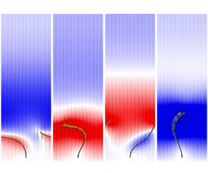
At the instant  $t^*/T^*=0$, the filament is undergoing the stroke reversal from the power to the recovery one. During this period, the filament reaches its leftmost position and is starting to flap rightward, as shown in figure 9(a). Under this condition, the filament moves slowly, resulting in the local minimum $P^*$ at around this instant, as shown in figure 8(b). Due to the flow inertia, only the flow closely wrapping the filament is along the positive $x$ direction, while that in the rest region goes in the opposite direction. Hence, $Q^*$ approaches a large negative value, i.e. $Q^*=-6.38$, at this instant, as shown in figure 8(a).
Contours of the  $x$ velocity ( $u^*$) in the $y^*=0$ plane (first row) and in the $z^*=0.7$ plane (second row) in the baseline case where ${F}_t^*=40$, $n=1$ and $Re=0.2$ at the instant $t^*/T^*=0$ (a), $t^*/T^*=0.25$ (b), $t^*/T^*=0.5$ (c) and $t^*/T^*=0.75$ (d).

As time advances to  $t^*/T^*=0.25$, the filament is beating rightward roughly with the maximum speed during the recovery stroke, as shown in figure 9(b). This leads to the local maximum $P^*$ at around this instant, as shown in figure 8(b). Compared with that at the instant $t^*/T^*=0$, more flow is directed by the filament towards the positive $x$ direction with larger speed. Meanwhile, the negative $x$-direction flow is slowed down and the corresponding region shrinks. As such, the flow rate reduces to $Q^*=-0.81$ at this instant.
At around the instant  $t^*/T^*=0.5$, the filament approaches the other stroke reversal, as shown in figure 9(c). Accordingly, $P^*$ reaches the other local minimum, as shown in figure 8(b). Compared with that at around $t^*/T^*=0.25$, the interface between the positive and negative $x$-direction flow regions approximately rises to $z^*=1.8$, while the flow in both regions becomes slower. As a result, the overall flow goes in the positive $x$ direction with $Q^* = 2.03$ at this instant. This explains why the mean effectiveness $\xi =-0.75$ rather than $-$1 in this case, as given in figure 6(b-v).
As time progresses to  $t^*/T^*=0.75$, the filament is beating leftward approximately with the maximum speed during the power stroke, as shown in figure 9(d). As such, $P^*$ approaches the other local maximum at around this instant, as shown in figure 8(b). Since the filament is the least bent and the most vertical at around this instant, it generally produces the strongest nearby flow within the whole beating period, if comparing the $x$-velocity contours at the four selected instants shown in figure 9. Moreover, the flow within the entire domain moves in the negative $x$ direction. Hence, $Q^*$ rapidly reaches the negative maximum, i.e. $Q^*=-8.44$, at $t^*/T^*=0.87$, as shown in figure 8(a).
3.2.3. Effects of follower-force magnitude
Figure 10 shows the beating patterns in the baseline case where the follower force  ${F}_t^*=40$ as well as three other cases with ${F}_t^*=30$, 50 and 60 when the power-law index $n=1$ and the Reynolds number $Re=0.2$. It is seen that, as ${F}_t^*$ increases, the filament beating pattern becomes wider in the $x$ direction and slightly shorter in the $z$ direction. This variation is the most obvious when ${F}_t^*$ augments from 30 to 40, whereas it turns less visible for larger ${F}_t^*$, as it is constrained by the negligible extensibility of the filament. Accordingly, the time-averaged flux ( $\bar {Q}^{*}$) is enhanced from $-$0.64 to $-$0.97 as $F_t^*$ increases from 30 to 40, while it remains at around $-$1.0 as $F_t^*$ further rises, as shown in the second row of figure 6. This implies that $|\bar {Q}^{*}|$ is positively correlated with the beating amplitude, and the effects of $F_t^*$ on them become saturated when it is sufficiently large. Furthermore, a larger $F_t^*$ can drive the filament to beat faster, which causes the stronger oscillation of the flow rate ( $Q^*$) and the higher input power ( $P^*$), as shown in figure 8.
Beating patterns of the curved filament in the cases with  $F_t^*=30$ (a), $F_t^*=40$ (b), $F_t^*=50$ (c) and $F_t^*=60$ (d) when $n=1$ and $Re=0.2$. Note that the filament number in each panel is arbitrary and is not related to $\,f^*$. The same applies to the other figures showing filament beating patterns.

3.2.4. Effects of power-law index
To unveil the influences of the power-law index ( $n$), the baseline case (where $n=1$ and the flow is Newtonian) as well as two representative non-Newtonian cases, i.e. the cases with $n=0.75$ and $n=1.5$ (corresponding to the shear-thinning and shear-thickening flows, respectively) when the follower force ${F}_t^*=40$ and the Reynolds number $Re=0.2$, are selected for detailed investigation.
Figure 11 shows that the filament beating pattern is similar but the beating amplitude increases as  $n$ increases from 0.75 to 1.5. The reason can be revealed from figure 12 through examining the competition of three types of forces in the $x$ direction along which the major deformation of the filament occurs, namely, the $x$-component follower force ( ${F}_{tx}^{*}$), the dimensionless drag force ( ${{F}_{D}^{*}}$) and the $x$-component inertial force which can be represented by that at the filament tip ( ${F}_{ix}^{*}$). ${{F}_{D}^{*}} = {F}_{D}{{T}_{r}^{n}}/{\kappa }{{L}_{c}^{2}}$, where ${F}_{D}$ is the $x$ component of the hydrodynamic force acting on the filament and is evaluated through the IBM (Gsell et al. Reference Gsell, D'Ortona and Favier2019), and ${F}_{ix}^{*} = -{m}^{*}{Re}({{\partial }^{2}{X^{*}_{1}}}/{{\partial }{t}^{*2}})$, where $X^{*}_{1}$ is the $x$ coordinate of the filament tip according to the first term of (2.10).
Beating patterns of the curved filament in the cases with  $n=0.75$ (a) and $n=1.5$ (c) as well as the baseline case where $n=1$ (b) when ${F}_t^*=40$ and $Re=0.2$.

Time histories of (a) the  $x$-component follower force ( $F_{tx}^*$), (b) the $x$-component inertial force at the filament tip ( $F_{ix}^*$) and (c) the drag force ( $F_{D}^*$) in the cases with $n=0.75$, 1 and 1.5 when $Re=0.2$ and ${F}_t^*=40$.

In these cases,  ${F}_{tx}^{*}$ is roughly independent of $n$, while ${F}_{D}^{*}$ is nearly anti-phase with ${F}_{tx}^{*}$ and generally has an amplitude comparable to that of ${F}_{tx}^{*}$, as shown in figure 12. In contrast, ${F}_{ix}^{*}$ is greatly dependent of $n$, and its amplitude decreases with $n$, as shown in figure 12(b). This stems from the fact that the drag-force amplitude can be generally scaled as ${F}_{DA}^{*} \sim ({\zeta }{u}_{m}^{*})^{n}$, where ${u}_{m}^{*}$ is the maximum nominal filament beating speed in the $x$ direction, and ${\zeta }$ is a constant determined by the filament geometry, as will be shown in § 5. If assuming that the filament generally undergoes a sinusoidal oscillation with the nominal beating amplitude of half the filament length, ${u}_{m}^{*} \sim {\rm \pi}f^*$, where $\,f^*$ is the beating frequency. Hence, ${F}_{DA}^{*} \sim ({{\rm \pi} }{\zeta }f^{*})^{n}$. As such, when the drag-force amplitude is the same, the filament has to beat faster in the shear-thinning flow ( $n<1$) and slower in the shear-thickening ( $n > 1$) flow than in the Newtonian flow ( $n=1$), as also evidenced by figures 9, 13 and 14 (refer to § 5 for more accurate and detailed explanations). Since a faster beating commonly corresponds to a larger acceleration and thus a greater inertial force, it is reasonable to see that the ${F}_{ix}^{*}$ amplitude decreases with $n$. As ${F}_{tx}^{*}$ and ${F}_{ix}^{*}$ are roughly anti-phase, their resultant force, which can be regarded as the effective actuation force, generally increases with $n$. Thus, a wider beating pattern presents at a higher $n$. These analyses show that the increase of $n$ is equivalent to that of $F_t^*$ when the structure inertia is not negligible.
Contours of the  $x$ velocity ( $u^*$) in the $y^*=0$ plane (first row) and in the $z^*=0.7$ plane (second row) in the case with ${F}_t^*=40$, $n=0.75$ and $Re=0.2$ at the instant $t^*/T^*=0$ (a), $t^*/T^*=0.25$ (b), $t^*/T^*=0.5$ (c) and $t^*/T^*=0.75$ (d).

Contours of the  $x$ velocity ( $u^*$) in the $y^*=0$ plane (first row) and in the $z^*=0.7$ plane (second row) in the case with ${F}_t^*=40$, $n=1.5$ and $Re=0.2$ at the instant $t^*/T^*=0$ (a), $t^*/T^*=0.25$ (b), $t^*/T^*=0.5$ (c) and $t^*/T^*=0.75$ (d).

Due to the different fluid-filament dynamics, the time histories of the flow rate ( ${Q}^{*}$) and input power ( ${P}^{*}$) are distinct in these cases, as shown in figure 15. In particular, as the filament beating speed in the case with $n=0.75$ is much larger than that in the baseline case, ${P}^*$ is generally larger (see figure 15b) and the ambient fluid speed is higher in the case with $n=0.75$. Owning to the shear-thinning behaviour, however, the fluid velocity decays much faster in space in the case with $n=0.75$, suggesting a smaller viscous length scale, as shown in figure 13. Therefore, only the flow closely surrounding the filament is evidently directed, and the oscillation of ${Q}^{*}$ is weaker. Also for this reason, a strong unidirectional flow right above the filament is developed in the case with $n=0.75$, which does not emerge in the baseline case. Consequently, the flow is always in the negative $x$ direction in the case with $n=0.75$, as shown in figure 15(a).
Time histories of the (a) flow rate ( $Q^*$) and (b) input power ( $P^*$) in the baseline case where $n=1$ and the cases with $n=0.75$ and 1.5 when ${F}_t^*=40$ and $Re=0.2$.

The influences of the shear-thickening behaviour on the filament and fluid dynamics are opposite to those of the shear-thinning one, as demonstrated in figures 9, 13 and 14. In the case with  $n=1.5$, the filament beats the most slowly, leading to the smallest ${P}^*$, as shown in figure 15(b). While a unidirectional flow is observed above the filament in the cases with $n=0.75$ and 1, in that with $n=1.5$ the viscous length scale is larger and the flow is oscillating across the whole domain. However, a clear phase lag develops in the $z$ direction, as shown in figure 14. The flow rate is generally smaller with larger oscillations than those in the other two cases, indicating that the flow transport is the least effective in the case with $n=1.5$, as shown in figure 15.
Although it is expected that the increase of the beating amplitude could enhance the absolute time-averaged flux ( $|\bar {Q}^{*}|$), as discussed in § 3.2.3, the opposite is true in this section. This implies the existence of a mechanism enhancing the flow transport in the shear-thinning case, despite the smaller beating amplitude. It could be related to the drastic variation of the viscous length scale with $n$, as shown in figures 9, 13 and 14. In the shear-thinning case, the length scale is the smallest, resulting in the presence of the unidirectional flow right above the filament and maximizing $|\bar {Q}^{*}|$.
3.2.5. Effects of Reynolds number
Figure 16 shows the filament beating pattern in the cases with the Reynolds number  $Re=0.04$, 0.2, 1 and 5 when the follower force ${F}_t^*=40$ and the power-law index $n=1$. It is noted that the beating amplitude and the time-averaged flux ( $\bar {Q}^{*}$) generally decrease with $Re$. This stems from that the $x$-component follower force ( ${F}_{tx}^{*}$) is roughly independent of $Re$, while the $x$-component inertial force ( ${F}_{ix}^{*}$) is generally anti-phase with ${F}_{tx}^{*}$ and its strength increases with $Re$. As such, their resultant force, i.e. the effective actuation force, diminishes with $Re$, as shown in figure 17. Hence, the increase of $Re$ is similar to reducing ${F}_t^*$ in § 3.2.3. Also for this reason, the filament beats slowly when $Re$ is large, and the oscillation amplitude of the input power ( $P^*$) turns smaller with $Re$, as shown in figure 18(b).
Beating patterns of the curved filament in the cases with  $Re=0.04$ (a), $Re=0.2$ (b), $Re=1$ (c) and $Re=5$ (d) when $n=1$ and $F_t^*=40$.

Time histories of (a) the  $x$-component follower force ( $F_{tx}^*$) and (b) the $x$-component inertial force at the filament tip ( $F_{ix}^*$) in the cases with $Re=0.04$, 0.2, 1 and 5 when $n=1$ and ${F}_t^*=40$.

Time histories of the (a) flow rate ( $Q^*$) and (b) input power ( $P^*$) in the cases with $Re=0.04$, 0.2, 1 and 5 when $n=1$ and ${F}_t^*=40$.

As  $Re$ increases, the viscous length scale decreases, and the region within which the fluid can be aligned with the beating filament shrinks, as evidenced by figure 19. This variation is quite similar to that when the flow goes from shear thickening to shear thinning, as discussed in § 3.2.4. As such, the oscillation amplitude of the flow rate ( $Q^*$) is reduced, as shown in figure 18(a). Furthermore, it is interesting to note that, even at $Re=0.04$, the fluid close to the top wall does not move synchronously with the filament, indicating that the inertial effects cannot be neglected in the corresponding region, as shown in figure 19(a). Similar findings have also been reported by Wei et al. (Reference Wei, Dehnavi, Aubin-Tam and Tam2021).
Contours of the  $x$ velocity ( $u^*$) in the $y^*=0$ plane (first row) and in the $z^*=0.7$ plane (second row) in the cases with $Re=0.04$ (a), $Re=0.2$ (b), $Re=1$ (c), $Re=5$ (d) when ${F}_t^*=40$ and $n=1$ at the instant $t^*/T^*=0.25$.

4. Flow transport at $Re \approx 0$

Extremely low-Reynolds-number flow, where  $Re$ is small enough to satisfy the creeping-flow condition, is attracting considerable attention due to extensive biological applications such as mucociliary transport and inspired potential engineering applications such as flow transport in microfluidic devices. Although numerical simulations at such low $Re$ are not conducted due to high computational cost, a scaling analysis together with the discussion in the previous section can provide useful insights into the filament dynamics and the flow transport under this circumstance.
4.1. Effects of Reynolds number
Equations (2.10) and (2.12) show that, when  $Re \approx 0$, the inertial terms in both equations become negligible, meaning that the dynamics of such a fluid-filament system is no longer affected by the variation of $Re$.
$Re$.
4.2. Effects of follower-force magnitude and power-law index
Similarly to the low- $Re$ regime, the filament dynamics at $Re \approx 0$ can be represented by the beating amplitude and the beating frequency ( $\,f^*$), while the flow transport can be represented by the time-averaged flux ( $\bar {Q}^*$), the time-averaged input power per unit area ( $\bar {P}^*$), the oscillation amplitudes of the flow rate and input power ( ${Q}^*_A$ and ${P}^*_A$), the transport efficiency ( $\eta$) and the mean effectiveness ( $\xi$). How these quantities are influenced by the follower-force magnitude ( $F_t^*$) and the power-law index ( $n$) in this regime is discussed in detail below.
4.2.1. Beating amplitude
When the filament achieves the maximum deformation, its velocity is close to zero. In the absence of inertia, the drag force turns negligible at such an instant, and thus the beating amplitude is expected to be only governed by a balance between  $F_t^*$ and the bending moment ( $M^*$). Since a larger $F_t^*$ can cause a greater $M^*$ which requires a larger deformation, the beating amplitude increases with $F_t^*$ at $Re \approx 0$, similarly to when $Re\ge 0.04$. In contrast, the effect of $n$ is expected to be negligible. This also corroborates the analysis performed in § 3.2.4, which suggests that the influence of $n$ on the beating amplitude is highly associated with that on the inertial force.
4.2.2. Beating frequency
At  $Re \approx 0$, the inertial force ( $F_i^*$) is neglected. Under this condition, the actuation force needs to be balanced by the drag force, i.e. $F_t^* \sim F_{DA}^*$, where $F_{DA}^*$ is the drag-force amplitude. As §§ 3.2.4 and 5 show that ${F}_{DA}^{*} \sim ({{\rm \pi} }{\zeta }f^{*})^{n}$, $\,f^*$ can be scaled as
 \begin{equation} f^{*} \sim \frac{(F_t^*)^{{1}/{n}}}{{\rm \pi} \zeta}, \end{equation}
where  $\zeta$ is a geometry-dependent constant. Thus, $\,f^*$ increases with $F_t^*$. As $F_t^*$ has to be much larger than 1 to trigger the dynamic instability, $\,f^*$ decreases with $n$, just as in the low- $Re$ regime.
4.2.3. Time-averaged flux
In the  $Re \approx 0$ regime, the viscous length scale is much larger than the distance between two adjacent filaments. Hence, the flow can be instantaneously directed by the filament, and its velocity is nearly the same as the filament beating velocity. Under this circumstance, it is reasonable to suppose that the shear stress in the $x$ direction is evenly distributed on the bottom wall, and the absolute mean shear stress can be written as
 \begin{equation} |\bar{\sigma}^{*}|=\frac{|\bar{F}_F^*|}{L^{*}W^{*}}, \end{equation}
where  $|\bar {F}_F^*|$ is the absolute time-averaged friction force on the bottom wall in the $x$ direction, and $L^{*}$ and $W^{*}$ are the length and width of the computational domain, corresponding to the filament spacing in the $x$ and $y$ directions, respectively.
According to the power-law model,  $|\bar {\sigma }^{*}|$ can be scaled as
 \begin{equation} |\bar{\sigma}^{*}| \sim |\bar{U}^{*}|^{n}, \end{equation}
where  $|\bar {U}^{*}|$ is the absolute time-averaged flow velocity and equals the absolute time-averaged flux ( $|\bar {Q}^*|$) according to (2.14). As such,
 \begin{equation} |\bar{Q}^{*}| \sim |\bar{\sigma}^{*}|^{{1}/{n}}. \end{equation}
Additionally, the time-averaged spatial integration of the momentum equation over the whole computational domain yields
 \begin{equation} |\bar{F}_D^*| = |\bar{F}_F^*|, \end{equation}
where  $|\bar {F}_D^*|$ is the absolute time-averaged drag force on the filament, it is defined as $|\bar {F}_D^*| = |\int _{{T}^{*}}{F}_{D}^{*}\, {\rm d} {t}^{*}/T^*|$, ${F}_D^*$ is the instantaneous drag force and $T^*$ is the filament beating period. Considering $|{F}_D^*| \sim ({{\rm \pi} }{\zeta }f^{*})^{n}$ at $Re \approx 0$, it could be assumed that
 \begin{equation} |\bar{F}_D^*| \sim {\phi}({\rm \pi}{\zeta}{f}^{*})^{n}, \end{equation}
where  ${\phi }$ is a non-negative asymmetry-dependent constant that is expected to be much smaller than 1. In general, the more asymmetric the beating pattern is, the larger ${\phi }$ is. As such, (4.4) can be rewritten as
 \begin{equation} |\bar{Q}^{*}| \sim {\rm \pi}{\zeta}{f^*}\left(\frac{\phi}{L^{*}W^{*}}\right)^{{1}/{n}}. \end{equation}
This suggests that  $|\bar {Q}^{*}|$ is proportional to ${\,f^*}$, which is generally in accord with that in the low- $Re$ regime.
Furthermore, (4.1) and (4.7) give rise to
 \begin{equation} |\bar{Q}^{*}| \sim \left(\frac{{\phi}F_t^*}{L^{*}W^{*}}\right)^{{1}/{n}}, \end{equation}
meaning that  $|\bar {Q}^{*}|$ increases with $F_t^*$ for a certain $n$, similarly to the low- $Re$ regime. On the other hand, the influence of the fluid rheology on $|\bar {Q}^{*}|$ depends on the value of ${{\phi }F_t^*}/{L^{*}W^{*}}$. Generally, $|\bar {Q}^*|$ decreases with $n$ at ${{\phi }F_t^*}/{L^{*}W^{*}}>1$, increases with $n$ at ${{\phi }F_t^*}/{L^{*}W^{*}}<1$ and is independent of $n$ at ${{\phi }F_t^*}/{L^{*}W^{*}}=1$. Therefore, if filaments are densely packed, beat in a sufficiently asymmetric manner, and $F_t^*$ is large enough, ${{\phi }F_t^*}/{L^{*}W^{*}}$ can be larger than 1. Under this condition, flow transport can be enhanced by shear-thinning behaviour. If the opposite is true, it can be improved by shear-thickening behaviour.
In nature, cilia usually undergo apparently asymmetric beating in bundles, and their spacing is much smaller than their length (Sleigh et al. Reference Sleigh, Blake and Liron1988; Schweickert et al. Reference Schweickert, Weber, Beyer, Vick, Bogusch, Feistel and Blum2007), i.e.  $L^*W^*\ll 1$. Considering that $F_t^*$ can be up to 120 for the cilia on eukaryotic cells (De Canio, Lauga & Goldstein Reference De Canio, Lauga and Goldstein2017), ${{\phi }F_t^*}/{L^{*}W^{*}}$ can be larger than 1 with great possibilities. Under this circumstance, if the ambient fluid exhibits shear-thinning behaviour, such as mucus in the human respiratory system, cilia could take this opportunity to enhance the flow transport.
4.2.4. Oscillation amplitude of flow rate
Section 3 reveals that in the low- $Re$ regime the oscillation amplitude of the flow rate ( ${Q}^*_A$) mainly depends on two factors, i.e. the viscous length scale within which the ambient fluid can be directed by the filament as well as the filament beating speed. At $Re \approx 0$, the viscous length scale is overwhelmingly large. Thus, the fluid can always be directed by the filament throughout the entire domain. As such, the influence of the first factor is negligible, and ${Q}^*_A$ only depends on the filament beating speed. If the maximum nominal filament beating speed in the $x$ direction is ${u}_{m}^{*}$, ${Q}^*_A$ can be scaled as
 \begin{equation} {Q}^{*}_{A} \sim {H}^{*}{W}^{*}{u}_{m}^{*} \sim {\rm \pi}{H}^{*}{W}^{*}{f}^{*}, \end{equation}
considering  ${u}_{m}^{*} \sim {\rm \pi}f^*$ as discussed in § 3.2.4, where $H^*$ is the height of the computational domain. Substituting (4.1)–(4.9) yields
 \begin{equation} {Q}^{*}_{A} \sim \frac{{H}^{*}{W}^{*}(F_t^*)^{{1}/{n}}}{\zeta}, \end{equation}
meaning that  ${Q}^*_A$ increases with the increase of $F_t^*$ or the decrease of $n$.
$n$.
4.2.5. Input power
The instantaneous input power ( $P^*$) exhibits two peaks and two troughs over each beating period in the low- $Re$ regime, and it nearly remains positive and always approaches zero near the troughs during the stroke reversals, as shown in figures 8, 15 and 18. This variation trend indicates that the time-averaged input power is generally proportional to the oscillation amplitude ( ${P}^{*}_{A}$), and this relation is expected to hold in the $Re \approx 0$ regime. Since ${P}^{*} = {\boldsymbol {F}_{t}^{*}} \boldsymbol {\cdot } {\boldsymbol {v}_{t}^{*}}$, where $\boldsymbol {F}_{t}^{*}$ is the follower-force vector and $\boldsymbol {v}_{t}^{*}$ is the filament-tip velocity vector, ${P}^{*}_{A}$ and the time-averaged input power per unit area ( $\bar {P}^*$) can be scaled as
 \begin{equation} {P}^{*}_{A} \sim \bar{P}^{*}{L}^{*}{W}^{*} \sim {\rm \pi}{F}^{*}_{t}{f}^{*} \sim \frac{(F_t^*)^{1+{1}/{n}}}{\zeta}. \end{equation}
Hence,  ${P}^{*}_{A}$ and $\bar {P}^{*}$ increase as $F_t^*$ increases or as $n$ decreases, similarly to the low- $Re$ regime.
4.2.6. Transport efficiency and mean effectiveness
Based on (2.16), (4.7) and (4.11),  $\eta$ can be scaled as
 \begin{equation} {\eta} \sim \frac{{\zeta}{\phi}^{1+{1}/{n}}}{({L^{*}W^{*}})^{{1}/{n}}}. \end{equation}
This relation implies that if  $n<1$, i.e. the flow is shear thinning, the closer the filaments are, i.e. the smaller $L^{*}W^{*}$ is, the higher the transport efficiency is.
As the flow is expected to be aligned by the filament all the time in the  $Re \approx 0$ regime due to the large viscous length scale, the flow cannot be unidirectional. Considering that the power stroke occurs when the filament moves leftward in this study, the mean effectiveness ( $\xi$) falls between $-$1 and 0.
Although the effects of  $F_t^*$ and $n$ on the filament and fluid dynamics are roughly similar in the two regimes, the scaling analysis conducted above is not directly applicable in the low- $Re$ one, since the inertial effects can be important. For instance, the viscous length scale is comparable to or much smaller than the filament spacing in the low- $Re$ regime. Therefore, the shear stress cannot be assumed to be evenly distributed on the bottom wall, which could nullify the scaling in (4.4) and the following.
4.3. Effects of viscosity
For the practical application of mucociliary transport, the fluid (mucus) viscosity varies in a wide range (Lai et al. Reference Lai, Wang, Wirtz and Hanes2009). Hence, it is also interesting and meaningful to examine how the viscosity influences the flow transport of the instability-driven filament. Herein, the power-law consistency index  $\kappa$ (which becomes the dynamic viscosity when $n=1$) is taken as the nominal viscosity, while $n$ is fixed. According to table 1, ${{F}_{t}^{*}}$ is defined by
 \begin{equation} {{F}_{t}^{*}} = \frac{{F}_{t}{{T}_{r}^{n}}}{{\kappa}{{L}_{c}^{2}}}, \end{equation}
where  $F_t$ is the dimensional follower-force magnitude, $T_r$ is the reference time scale and $L_c$ is the filament length. Substituting (2.9) into (4.13) yields
 \begin{equation} {{F}_{t}^{*}} = \frac{{F}_{t}{{L}_{c}^{2}}}{EI}, \end{equation}
where  $EI$ denotes the bending stiffness. Assuming that $L_c$, $EI$ and ${F}_{t}$ are constant and irrelevant to $\kappa$, ${F}_{t}^{*}$ is fixed and is also independent of $\kappa$. As the beating frequency $\,f^*$ only depends on ${{F}_{t}^{*}}$ in the $Re \approx 0$ regime when $n$ is fixed, $\,f^*$ is unrelated to $\kappa$. Substituting (2.9) into (2.13) gives rise to the dimensional frequency
 \begin{equation} {f} = \left(\frac{EI}{\kappa{L_c^4}}\right)^{{1}/{n}}{f^*}, \end{equation}
meaning that  $f$ is only a function of $\kappa$ and is proportional to $1/\sqrt [\leftroot {-2}\uproot {2}n]{\kappa }$. Hence, $f$ diminishes with $\kappa$. The decrease of $f$ suggests the reduction of the filament beating speed, since the beating amplitude which is mainly determined by ${{F}_{t}^{*}}$ remains unchanged. This results in the decrease of the dimensional time-averaged flux and input power with the increase of $\kappa$.
The above analysis agrees well with in vitro experimental observation (Gheber, Korngreen & Priel Reference Gheber, Korngreen and Priel1998) in terms of the variation trend of  $f$ with the viscosity. However, Gheber et al. (Reference Gheber, Korngreen and Priel1998) demonstrated the dependence of the beating pattern on the viscosity, differing from the independent relation found in this study, as partly evidenced by figure 16 showing that the filament beating pattern nearly remains the same as $Re$ increases from 0.04 to 0.2. Such a discrepancy may result from that, compared with those in in vitro experiment, several factors are neglected in the current numerical model, such as more complex ciliary dynamics, ciliary coordination and fluid heterogeneity.
5. Linear stability analysis
The previous section reveals that the beating frequency ( $\,f^*$) is closely correlated with the time-averaged flux ( $\bar {Q}^{*}$) and the time-averaged input power per unit area ( $\bar {P}^{*}$). Thus, it is an important indicator for flow transport induced by an instability-driven filament. In this section, a linear stability analysis is conducted to reveal how $\,f^*$ is affected by three parameters, i.e. the power-law index ( $n$), the follower force ( ${F}_t^*$) and the Reynolds number ( $Re$), from a theoretical point of view.
In this study, the follower force imposed at the filament tip is non-conservative due to the fact that it keeps changing its direction as the filament flaps (Timoshenko & Gere Reference Timoshenko and Gere1961). Under this condition, the dynamic criterion of stability is required in the analysis. Such a kind of analysis on an inertial-force-dominated system has been done in Timoshenko & Gere (Reference Timoshenko and Gere1961), while that on a viscous-force-dominated Newtonian creeping-flow system has been conducted in De Canio et al. (Reference De Canio, Lauga and Goldstein2017). Herein, this analysis is extended to a problem simultaneously involving the inertial and viscous forces in a power-law-model-based generalized-Newtonian flow.
Assuming that the filament is inextensible, and that it is straight in its zero-stress state and only undergoes small deformation, the governing equation for the filament dynamics can be written as (Timoshenko & Gere Reference Timoshenko and Gere1961)
 \begin{equation} {EI}\frac{{\partial}^{4}{x}}{{\partial}{z}^{4}} + {F}_{t}\frac{{\partial}^{2}{x}}{{\partial}{z}^{2}} = {F}_{E}, \end{equation}
where  $EI$ is the bending stiffness and ${F}_{E}$ is the lateral loading per unit length acting on the filament. In this study, ${F}_{E}$ consists of two components. One is the inertial force of the filament, which is expressed as
 \begin{equation} {F}_{I} ={-}{\rho}_{c}{A}\frac{{\partial}^{2}{x}}{{\partial}{t}^{2}}, \end{equation}
according to d’Alembert's principle, where  ${\rho }_{c}$ and $A$ are the filament density and cross-section area, respectively. The other is the hydrodynamic force, i.e. the drag force. According to the resistive-force theory in the absence of background flow, it can be evaluated as (De Canio et al. Reference De Canio, Lauga and Goldstein2017)
 \begin{equation} {F}_{D} ={-}{\beta}{\mu}\frac{{\partial}{x}}{{\partial}{t}}, \end{equation}
if the flow is creeping and Newtonian, where  $\mu$ is the dynamic viscosity, ${\beta }=4{\rm \pi} /[\text {ln}(L_c/D)+1/2]$, and $L_c$ and $D$ are the filament length and diameter, respectively.
Riley & Lauga (Reference Riley and Lauga2017) extended the resistive-force theory to the Carreau-model-based shear-thinning flow. Specifically, they made a locally Newtonian assumption and found that the average shear rate on the surface of a rod can be estimated as
 \begin{equation} \dot{\gamma}_{avg} = \frac{{\beta}{u}_{\dot{\gamma}}}{\sqrt{2} D {\rm \pi}}, \end{equation}
where  ${u}_{\dot {\gamma }}$ is the shear rate velocity. Then, they replaced the shear rate ( $\dot {\gamma }$) in the Carreau model with $\dot {\gamma }_{avg}$ to estimate the dynamic viscosity and drag force.
Inspired by Riley & Lauga (Reference Riley and Lauga2017), the aforementioned approach is extended to the power-law-model-based generalized-Newtonian flow in this study. Since the filament is inextensible and its deflection is small by assumption, the major component of the velocity is perpendicular to the filament axis. Thus,  ${u}_{\dot {\gamma }}$ is approximated as $|{{\partial }{x}}/{{\partial }{t}}|$. As such, the drag force can be expressed as
 \begin{equation} {F}_{D} ={-}{\kappa}{\beta}^{n}({\sqrt{2}{\rm \pi} D})^{1-n}{\left|\frac{{\partial}{x}}{{\partial}{t}} \right|}^{n-1}\frac{{\partial}{x}}{{\partial}{t}}. \end{equation}
When  $n=1$, (5.5) recovers (5.3). Although the drag-force modelling is based on the assumption that the background flow is creeping and stationary, it is hypothesized that (5.5) is roughly valid even when the flow is slightly inertial and time dependent.
Substituting (5.2) and (5.5) into (5.1) which is then parameterized with the three repeating variables selected in § 2.1, i.e. the fluid density ( ${\rho }_{f}$), the reference time scale ( ${T}_{r}$) and ${L}_{c}$, gives rise to
 \begin{equation} {m}{Re}\frac{{\partial}^{2}{x}}{{\partial}{t}^{2}} + \frac{{\partial}^{4}{x}}{{\partial}{z}^{4}} + {\alpha}\frac{{\partial}{x}}{{\partial}{t}} + {{F}_{t}}\frac{{\partial}^{2}{x}}{{\partial}{z}^{2}} = 0, \end{equation}
where  ${\alpha } = {\beta }^{n}({\sqrt {2} {\rm \pi}{D}})^{1-n}{|{{\partial }{x}}/{{\partial }{t}}|}^{n-1}$ represents the fluid damping coefficient, and $EI=1$ (see table 1) has been substituted. The third term in this equation means that the absolute non-dimensional drag force can be roughly scaled as $|{F}_{D}| \sim {({\zeta }|{{\partial }{x}}/{{\partial }{t}}|)}^{n}$, as has been used in the previous sections, where ${\zeta }={\beta }/({\sqrt {2} {\rm \pi}{D}})$, and ${\zeta } \approx 10$ due to $D=0.1$ in this study, as given in table 1. Note that the stars of all the dimensionless parameters in (5.6) have been dropped, and this convention will be used henceforth for simplicity.
Since one end of the filament ( $z=0$) is clamped on the bottom surface, while the other end ( $z=1$) is free, the boundary conditions can be written as
 \begin{equation} x(t,0)=\frac{{\partial}{x}}{{\partial}{z}}(t,0)= \frac{{\partial}^2{x}}{{\partial}{z}^2}(t,1)= \frac{{\partial}^3{x}}{{\partial}{z}^3}(t,1)=0. \end{equation}
 In (5.6), all the terms are linear except the third one corresponding to the drag force. In order to perform the linear stability analysis, this term needs to be linearized. In particular,  ${\alpha }$ is calculated in the map of $|{{\partial }{x}}/{{\partial }{t}}|$ vs $n$, as plotted in figure 20(a). It is seen that ${\alpha }$ generally rises with $n$. When $n > 1$, ${\alpha }$ increases with $|{{\partial }{x}}/{{\partial }{t}}|$, whereas ${\alpha }$ decreases with $|{{\partial }{x}}/{{\partial }{t}}|$ when $n < 1$. At $n=1$, ${\alpha }$ remains constant, i.e. 4.48, meaning that it is independent of $|{{\partial }{x}}/{{\partial }{t}}|$ in Newtonian flow. More importantly, it is observed that, roughly at $|{{\partial }{x}}/{{\partial }{t}}| > 1$, the ${\alpha }$ contour line becomes relatively vertical, indicating that ${\alpha }$ depends much more on $n$ than $|{{\partial }{x}}/{{\partial }{t}}|$. The simulation results in § 3.1 reveal that the minimum absolute time-averaged velocity of the filament tip is 2.22 among all the cases. Under this circumstance, ${\alpha }$ can be approximately assumed to be independent of $|{{\partial }{x}}/{{\partial }{t}}|$, and it is precalculated at all $n$ given in table 1 with $|{{\partial }{x}}/{{\partial }{t}}|=2.22$ for the linearization. These $\alpha$ are defined as the effective fluid damping coefficient ( $\bar {\alpha }$), and the curve of $\bar {\alpha }$ vs $n$ is plotted in figure 20(b).
Contour of  $\alpha$ in the map of $|{{\partial }{x}}/{{\partial }{t}}|$ vs $n$ (a), and $\bar {\alpha }$ at different $n$ (b).

The linearized equation has a general solution which can be expressed as
 \begin{equation} x = [ {{C_1}\cosh ( {{\lambda _1}z} ) + {C_2}\sinh ( {{\lambda _1}z} ) + {C_3}\cos ( {{\lambda _2}z} ) + {C_4}\sin ( {{\lambda _2}z} )} ]\,{{\rm e}^{\omega t}}, \end{equation}
with
 \begin{equation} {\lambda}_{1} = \sqrt {\sqrt {\frac{{{F_t^2}} }{4} - ( {m{Re} {\omega^2} + \bar{\alpha} \omega} )} - \frac{{{F_t}}}{2}}, \end{equation}
and
 \begin{equation} {\lambda}_{2} = \sqrt {\sqrt {\frac{{{F_t^2}} }{4} - ( {m{Re} {\omega^2} + \bar{\alpha} \omega} )} + \frac{{{F_t}}}{2}}, \end{equation}
where  $\omega$ is a complex parameter, its real component $(Re(\omega ))$ represents the growth/decay rate subjected to a perturbation, while its imaginary component $(Im(\omega ))$ corresponds to the beating frequency $f={Im} (\omega /2{\rm \pi} )$.
Substituting (5.8) into (5.6) and imposing the boundary conditions given in (5.7) yield four linear algebra equations for the undetermined coefficient  $C_i$ where $i=1$ to 4. One solution of this linear system is $C_i=0$ for all $i$, meaning that the filament remains stationary all the time. This requires the existence of another solution according to the dynamic criterion of stability, for which the determinant of the corresponding coefficient matrix has to be zero. Hence
 \begin{align} &F_t^2 - 2{m}{Re} {\omega ^2} - 2\bar{\alpha} \omega + {F_t}\sqrt { - ( {{m}{Re} {\omega ^2} + \bar{\alpha} \omega } )}\sinh ( {{\lambda _1}} )\sin ( {{\lambda _2}} ) \nonumber\\ & \quad - 2({{m}{Re} {\omega ^2} + \bar{\alpha} \omega } )\cosh ( {{\lambda _1}} )\cos ( {{\lambda _2}} ) =0, \end{align}
from which  $\omega$ can be solved numerically. Taking the case with $n=1$ and $Re=0.2$ as an example, figure 21 shows the solution of (5.11) for this case as $F_t$ varies from 0 to 60 in terms of $Re(\omega )$ and $Im(\omega /2{\rm \pi} )$. It is seen that, in the range of $F_t=0$ to 20.06, $Re(\omega )$ is negative while $Im(\omega /2{\rm \pi} )$ remains at zero, meaning that the filament subjected to a perturbation exponentially recovers to its original shape without oscillation. When $F_t$ is between 20.06 and 37.3, $Re(\omega )$ remains negative while $Im(\omega /2{\rm \pi} )$ becomes positive, indicating that, once a perturbation is introduced, the filament will undergo oscillations with decayed amplitude and eventually return to its original shape. At $F_t$ larger than the critical value, i.e. 37.3, $Re(\omega )$ and $Im(\omega /2{\rm \pi} )$ are positive, meaning the onset of the dynamic instability. As such, the filament exhibits a self-sustained oscillation.
Real component of  $\omega$ $(Re(\omega ))$ and the oscillation frequency $(Im(\omega /2{\rm \pi} ))$ in the case with $n=1$ and $Re=0.2$ when ${F}_t$ varies from 0 to 60.

From figure 21,  $Im(\omega /2{\rm \pi} )$ at $F_t=40$, 50 and 60 is identified as 7.20, 9.01 and 11.32 respectively. In this way, $Im(\omega /2{\rm \pi} )$ in the cases involved in § 3.1 is determined and then plotted in figure 22. Note that it is observed that the dynamic instability is not triggered in most cases with $F_t = 30$ according to the stability analysis. Thus, they are not included in this figure. Comparing figure 2 with figure 22 shows that the contours attained from the DNS and the theoretical analysis are reasonably close, meaning that the effects of $n$,
$n$,  $F_t$ and $Re$ on the beating frequency can be predicted by the proposed linear stability analysis.
Interpolated contours of the theoretical dimensionless beating frequency ( $\,f=Im(\omega /2{\rm \pi} ))$ of the straight filament when the follower force ${F}_t^*=40$ (a), ${F}_t^*=50$ (b) and ${F}_t^*=60$ (c). Transparent symbols denote data points obtained from the linear stability analysis.

However, there also exist some evident discrepancies between the theoretical and numerical results. For instance, the analysis usually overestimates the critical value of  $F_t$ for the onset of the instability as well as the beating frequency. This mainly stems from the oversimplification of the adopted hydrodynamic force model, such as that the drag-force modelling based on the creeping-flow assumption is supposed to be valid despite the presence of inertial effects, as well as the simplified assumptions made for the linearization of this model.
Furthermore, figure 23 shows the contour of the absolute non-dimensional drag force ( $|{F}_{D}|$) in the map of $|{{\partial }{x}}/{{\partial }{t}}|$ vs $n$, according to the third term in (5.6). It can be seen that $|{F}_{D}|$ increases with $|{{\partial }{x}}/{{\partial }{t}}|$ and $n$. This, from a more accurate perspective, explains why the filament beats faster as the flow behaviour changes from shear thickening to shear thinning if $|{F}_{D}|$ roughly stays the same, as well as why the filament beating speed increases with $|{F}_{D}|$ at a given $n$, as discussed in the previous sections.
Contour of the theoretical absolute non-dimensional drag force ( $|{F}_{D}|$) in the map of $|{{\partial }{x}}/{{\partial }{t}}|$ vs $n$.
$n$.

6. Conclusion
This study extends our understanding on the transport of the power-law-based non-Newtonian fluid by the active beating of an instability-driven filament from numerical and theoretical perspectives. Two regimes are considered, i.e. the low- $Re$ and $Re \approx 0$ regimes, where inertial effects are present and negligible, respectively. The major findings are summarized below.
(i) In the low-
$Re$ regime where $Re=0.04$ to 5, the filament zero-stress shape represented by the arc angle $\theta$ does not have a significant influence on its beating frequency ($\,f^*$), but is crucial for the flow transport. Only when $\theta \neq 0$, i.e. the filament is curved in its zero-stress state, is the beating pattern asymmetric and yields a non-zero time-averaged flux ($\bar {Q}^{*}$).(ii) When
$\theta \neq 0$, the follower force ($F_t^*$) is a key factor in dictating the filament dynamics and the resulting flow transport. The value of $F_t^*$ determines the onset of the dynamic instability of the filament. In all cases, the critical $F_t^*$ is around 30. Once the instability sets in, the increasing $F_t^*$ enhances the beating amplitude and $\,f^*$, associated with the augmentation of the flow rate (${Q}^{*}$), the input power (${P}^{*}$) and their time- and space-averaged counterparts, i.e. $\bar {Q}^{*}$ and $\bar {P}^{*}$.(iii) The increase of
$Re$ enhances the filament inertial force which offsets $F_t^*$, resulting in the reduction of the effective actuation force. As such, the influences of $Re$ on the filament dynamics and the flow transport are generally opposite to those of $F_t^*$, i.e. the increase of $Re$ weakens the flow transport.(iv) The variation of the power-law index (
$n$) is also correlated with the alternation of the effective actuation force, i.e. the decrease of $n$ increases $\,f^*$, which thus globally amplifies the inertial force and weakens the effective actuation. Furthermore, as the viscous length scale reduces with the decrease of $n$, a unidirectional flow can be developed above the filament in the shear-thinning case, which enhances $\bar {Q}^{*}$. Considering that the transport efficiency ($\eta$) and the mean effectiveness ($\xi$) can also be improved by reducing $n$, the shear-thinning behaviour is more beneficial to the flow transport.(v) In the
$Re \approx 0$ regime, the scaling analysis shows that the effects of $F_t^*$ and $n$ are roughly the same as those in the low-$Re$ regime. Exceptions are that in this regime the beating amplitude is nearly independent of $n$ and the oscillation amplitude of ${Q}^{*}$ decreases with $n$.(vi) The linear stability analysis is performed by extending the resistive-force theory to the power-law-model-based generalized-Newtonian flow. The analysis shows that the variation of
$\,f^*$ with $F_t^*$, $n$ and $Re$ can be generally predicted. However, $\,f^*$ and the critical ${F}_t^*$ are overestimated due to the oversimplifications made in the analysis.


This study also provides some physical insights into ciliary transport in nature. In particular, the scaling analysis reveals that  $|\bar {Q}^{*}| \sim ({{\phi }F_t^*}/{L^{*}W^{*}})^{{1}/{n}}$, suggesting the influences of the fluid rheology on $|\bar {Q}^*|$ are determined by the value of ${{\phi }F_t^*}/{L^{*}W^{*}}$ where $\phi$ represents the asymmetry of the beating pattern. As it is expected that ${{\phi }F_t^*}/{L^{*}W^{*}}>1$ in the human respiratory system where mucus commonly exhibits shear-thinning behaviour ( $n<1$), cilia could make use of this fluid behaviour to enhance the flow transport. Furthermore, the scaling analysis reveals that the increase of the fluid viscosity can reduce the beating frequency, agreeing well with in vitro experimental observations (Gheber et al. Reference Gheber, Korngreen and Priel1998).
Although insightful, this study has some limitations. In nature and practical applications, the flow field and the fluid properties can be more complicated than those assumed herein. For instance, in mucociliary transport two layers of fluid are usually involved, including the low-viscosity periciliary layer and the high-viscosity mucus layer which can exhibit complex non-Newtonian behaviours, such as the viscoelastic behaviour. Moreover, cilia typically coordinate with their neighbours and manifest a collective behaviour, i.e. the metachronal wave. The flow transport of the instability-driven filament under these circumstances will be a subject of our near-future investigations.
Acknowledgements
The authors thank the Mesocenter of Aix Marseille University and CINES for granting accesses to the high performance computing resources.
Funding
This work was supported by the MACBION project, the Excellence Initiative of Ai $x$-Marseille University A*MIDEX (a French Investissements d'Avenir programme) and the SINUMER project of the French National Research Agency (grant number ANR-18-CE45-0009-01).
Declaration of interests
The authors report no conflict of interest.
Appendix. Convergence test
To guarantee the independence of the numerical results on the mesh and time-step resolutions, a series of convergence tests is performed. It is found that the resolution highly depends on the Reynolds number ( $Re$) and the power-law index ( $n$), i.e. the smaller $Re$ or the larger $n$, the finer resolution is usually required. Therefore, to avoid unnecessary computational cost as well as to ensure the numerical accuracy, the convergence tests are conducted at all $Re$ and $n$ involved in this study, i.e. $Re=0.04$, 0.2, 1 and 5, and $n=0.75$, 1, 1.25 and 1.5, when the follower force ${F}_{t}^{*}=40$ and the arc angle $\theta =3{\rm \pi} /4$.
Taking  $Re=0.2$ and $n=1$ as an example, four cases are selected for the convergence test, and four primary quantities are used for examining the convergence, including the beating frequency ( $\,f^*$), time-averaged flux ( $\bar {Q}^*$), time-averaged input power per unit area ( $\bar {P}^*$) and mean effectiveness ( ${\xi }$), as listed in table 2. Herein, it is assumed that the most accurate results are yielded by the finest mesh and time resolutions, i.e. ${{\rm \Delta} x} = {L_c}/80$ and ${{\rm \Delta} t}/{T_r} = 6.25 \times {10}^{-6}$, where ${T}_{r}$ is the reference time scale. If another set of ${{\rm \Delta} x}$ and ${{\rm \Delta} t}/{T_r}$ gives rise to results which differ by no more than 5 % when compared with the most accurate ones, the results are considered converged and such a set is adopted for the simulation. As such, the set of ${{\rm \Delta} x}={L_c}/40$ and ${{\rm \Delta} t}/{T_r} = 1.25 \times {10}^{-5}$ is identified when $Re=0.2$ and $n=1$. Those for other $Re$ and $n$ are determined in the same way and given in table 3.
Results for the convergence test at the Reynolds number  $Re=0.2$ and $n=1$, where ${T}_{r}$ is the reference time scale defined in (2.9).

Mesh spacing and non-dimensional time step at different  $Re$ and $n$.
$n$.


 Open access

