





1. Introduction
Transition to turbulence in hypersonic boundary layers (HBLs) has a profound impact on aerodynamic performance, thermal management and structural durability of high-speed air vehicles. The intense surface loading that arises within transitional and turbulent boundary layers imposes considerable constraints on vehicle design, often diminishing propulsive efficiency and impacting vehicle longevity and operability (Guo et al. Reference Guo, Shi, Gao, Jiang, Lee and Wen2022; Zhou et al. Reference Zhou, Liu, Lu, Wang and Yan2022). Therefore, understanding the mechanisms that initiate and sustain boundary layer transition, and devising strategies to mitigate or delay it, is imperative. Sensitivity of transition to an expansive parametric space makes this an extremely difficult task. This includes, influence of free stream conditions (Goldstein Reference Goldstein2014; Andrews & Poggie Reference Andrews and Poggie2020), thermal boundary conditions (BCs) (Wannenwetsch & Martindale Reference Wannenwetsch and Martindale1977; Araya et al. Reference Araya, Lagares, Santiago and Jansen2021; Unnikrishnan & Gaitonde Reference Unnikrishnan and Gaitonde2021), geometric features (Stetson Reference Stetson1983; Paredes et al. Reference Paredes, Choudhari, Li, Jewell, Kimmel, Marineau and Grossir2018; Goparaju, Unnikrishnan & Gaitonde Reference Goparaju, Unnikrishnan and Gaitonde2021), surface roughness (Schneider Reference Schneider2008; Shi et al. Reference Shi, Xu, Wang and Lv2019) and the spectral and fluid-thermodynamic characteristics of the surrounding disturbance environment (Reshotko Reference Reshotko1976; Balakumar & Chou Reference Balakumar and Chou2018).
Extensive research has been performed to study fundamental mechanisms of hypersonic transition using canonical geometries, including, flat plates (Sivasubramanian & Fasel Reference Sivasubramanian and Fasel2011; Unnikrishnan, Cavalieri & Gaitonde Reference Unnikrishnan, Cavalieri and Gaitonde2019), wedges (Balakumar Reference Balakumar2015), circular cones (Chou et al. Reference Chou, Ward, Letterman, Schneider, Luersen and Borg2011) and, more recently, flared cones (Hader & Fasel Reference Hader and Fasel2019; Zhang & Shi Reference Zhang and Shi2022), double cones (Fan, Hao & Wen Reference Fan, Hao and Wen2022) and cone–cylinder–flare (CCF) structures (Benitez et al. Reference Benitez, Borg, Paredes, Schneider and Jewell2023a ). While sharp flat-plate/straight-cone configurations are commonly utilized to research natural and controlled transition pathways, especially focusing on inherent instability modes, studies with flight-relevant geometries should expect added complexities. These include the impact of geometry-induced pressure gradients, nose-tip effects, the non-uniformity in base flow due to angle of attack and the strong viscous–inviscid interactions that substantially influence transition mechanisms. Such studies are necessary to extend our fundamental understanding of hypersonic transition to practical configurations, which may sustain interplay of multiple flow phenomena, that eventually determine realistic loading scenarios on the vehicle.
Using linear theory and scale-resolved simulations, the present work addresses the above necessity by studying the transitional and post-transitional dynamics, and wall loading over an idealized hypersonic geometry, which sustains multimodal mechanisms and their mutual interactions under certain operating conditions. Specifically, we study the flow dynamics over a CCF geometry inspired by the HIFiRE-1 experiments (Kimmel & Prabhu Reference Kimmel and Prabhu2015), under relatively low and high free stream perturbation levels. This geometry originally featured a blunted $7^\circ$
half-angle cone with an attached cylinder, and a
$7^\circ$
half-angle cone with an attached cylinder, and a $33^\circ$
flare configuration (Adamczak, Alesi & Frost Reference Adamczak, Alesi and Frost2009). While the cone–cylinder junction produces an expansion fan, the cylinder–flare junction creates a compression corner, resulting in an oblique shock. Due to the associated adverse pressure gradient, the boundary layer thickens and decelerates. The degree of adverse pressure gradient and the intensity of the oblique shock are highly dependent on the turning angle, and can drive separation of the incoming boundary layer at sufficiently large angles. This generates a shock–boundary layer interaction (SBLI) zone and a separation bubble, over which a shear layer develops. When present, the separation bubble can accelerate the onset of transition in the shear layer, potentially driving the flow to a fully turbulent state before reattachment in certain configurations (Paredes et al. Reference Paredes, Scholten, Choudhari, Li, Benitez and Jewell2022). This idealized geometry thus facilitates a rigorous study of several fundamental multimodal interactions that may occur in hypersonic flight vehicles, some of which are further detailed below.
$33^\circ$
flare configuration (Adamczak, Alesi & Frost Reference Adamczak, Alesi and Frost2009). While the cone–cylinder junction produces an expansion fan, the cylinder–flare junction creates a compression corner, resulting in an oblique shock. Due to the associated adverse pressure gradient, the boundary layer thickens and decelerates. The degree of adverse pressure gradient and the intensity of the oblique shock are highly dependent on the turning angle, and can drive separation of the incoming boundary layer at sufficiently large angles. This generates a shock–boundary layer interaction (SBLI) zone and a separation bubble, over which a shear layer develops. When present, the separation bubble can accelerate the onset of transition in the shear layer, potentially driving the flow to a fully turbulent state before reattachment in certain configurations (Paredes et al. Reference Paredes, Scholten, Choudhari, Li, Benitez and Jewell2022). This idealized geometry thus facilitates a rigorous study of several fundamental multimodal interactions that may occur in hypersonic flight vehicles, some of which are further detailed below.
Early work by Becker & Korycinski (Reference Becker and Korycinski1962) on an ogive–cylinder–flare model discusses SBLI-induced separation bubbles, and the impact of boundary layer conditions on bubble geometry, underscoring a strong relationship between the separation region and transitional flow dynamics. Subsequently, Ginoux (Reference Ginoux1965) investigated the CCF geometry experimentally, identifying streamwise vortices on the flare downstream of reattachment on a hollow cylinder–flare set-up. A notable outcome was that the conical forebody reduced the prominence of these vortices. These streamwise vortices correlated with high heat flux streaks at the wall near reattachment, and potentially triggered transition to turbulence. More recent work by Dwivedi et al. (Reference Dwivedi, Sidharth, Nichols, Candler and Jovanović2019) has further clarified that base-flow deceleration substantially amplifies streamwise velocity, while baroclinic effects generate streamwise vorticity. This study also revealed that temperature streaks near reattachment arise from the amplified growth of streamwise velocity and vorticity perturbations, compounded by the enhancement of upstream temperature perturbations, through the reattachment shock.
Due to the sufficiently high edge Mach number in the present study, the HBL may also sustain Mack’s second mode (Mack Reference Mack1990), which has been well-documented over canonical geometries like flat plates and slender cones. However, its interactions with separated regions are still not fully characterized. For example, Adams (Reference Adams, Liu, Sakell and Beutner2001) found that, over a compression ramp, the second mode did not amplify within a laminar separation bubble, whereas Balakumar, Zhao & Atkins (Reference Balakumar, Zhao and Atkins2005) observed its amplification postreattachment. Similar behaviour was noted in quiet tunnel experiments by Benitez et al. (Reference Benitez, Esquieu, Jewell and Schneider2020) on a CCF with a $10^{\circ}$
flare angle, where both second mode and shear layer instabilities appeared postreattachment. In this study, sufficiently large-amplitude broadband disturbance was introduced upstream of separation, resulting in the amplification of shear layer instabilities, and formation of convecting turbulent spots downstream, without fully undergoing transition. Further work by Paredes et al. (Reference Paredes, Scholten, Choudhari, Li, Benitez and Jewell2022) indicated that a slight increase in the flare angle could destabilize both shear and boundary layers sufficiently, to induce transition under low-disturbance conditions. Experiments by Benitez et al. (Reference Benitez, Borg, Paredes, Schneider and Jewell2023a
) using a
$10^{\circ}$
flare angle, where both second mode and shear layer instabilities appeared postreattachment. In this study, sufficiently large-amplitude broadband disturbance was introduced upstream of separation, resulting in the amplification of shear layer instabilities, and formation of convecting turbulent spots downstream, without fully undergoing transition. Further work by Paredes et al. (Reference Paredes, Scholten, Choudhari, Li, Benitez and Jewell2022) indicated that a slight increase in the flare angle could destabilize both shear and boundary layers sufficiently, to induce transition under low-disturbance conditions. Experiments by Benitez et al. (Reference Benitez, Borg, Paredes, Schneider and Jewell2023a
) using a $12^{\circ}$
flare angle in a quiet tunnel revealed an amplified shear layer mode in the frequency band of Mack’s first mode in the postreattachment region, and noted the re-emergence of the second mode over the flare, despite its dampening over the cylinder. They also observed turbulent spot formation, inferred to be generated by shear layer instability wave packets. Recently, Caillaud et al. (Reference Caillaud2024) applied resolvent analysis to study non-modal disturbance growth across various Reynolds numbers on sharp and blunt nose-tip CCF geometries, finding substantial amplification of the first and second modes in sharp-tip cases, while both were stabilized in the blunt-nose configurations. Their analysis identified a low-frequency instability mechanism similar to the first mode in the shear layer, and a high-frequency mechanism akin to the second mode within the separation bubble, for sharp-tip geometries.
$12^{\circ}$
flare angle in a quiet tunnel revealed an amplified shear layer mode in the frequency band of Mack’s first mode in the postreattachment region, and noted the re-emergence of the second mode over the flare, despite its dampening over the cylinder. They also observed turbulent spot formation, inferred to be generated by shear layer instability wave packets. Recently, Caillaud et al. (Reference Caillaud2024) applied resolvent analysis to study non-modal disturbance growth across various Reynolds numbers on sharp and blunt nose-tip CCF geometries, finding substantial amplification of the first and second modes in sharp-tip cases, while both were stabilized in the blunt-nose configurations. Their analysis identified a low-frequency instability mechanism similar to the first mode in the shear layer, and a high-frequency mechanism akin to the second mode within the separation bubble, for sharp-tip geometries.
Another factor that compounds flow complexity in the presence of the above instability dynamics is their sensitivity to free stream disturbance levels. This was evidenced in recent experiments conducted by Benitez et al. (Reference Benitez2024) on a blunt CCF at multiple facilities, where they observed differences in the reattachment location of the separation region, state of the boundary layer post reattachment and instabilities amplified in the flow, which were hypothesized to be caused due to differences in tunnel noise properties, among other factors. In the present case, while we expect some of the modal instabilities to define transitional pathways under low free stream perturbation amplitudes, non-modal or bypass mechanisms Morkovin (Reference Morkovin1985) may take over at sufficiently high perturbation amplitudes, circumventing the growth of primary and associated secondary modes. The penetration of low-frequency vortical disturbances into the boundary layer facilitated by high-frequency shielding phenomena (Hunt & Durbin Reference Hunt and Durbin1999; Zaki & Durbin Reference Zaki and Durbin2005), the resulting streak formation due to lift-up effects (Landahl Reference Landahl1980; Jacobs & Durbin Reference Jacobs and Durbin2001) and eventual turbulent spot generation through secondary instabilities (Andersson et al. Reference Andersson, Brandt, Bottaro and Henningson2001; Ovchinnikov, Choudhari & Piomelli Reference Ovchinnikov, Choudhari and Piomelli2008) could result in potential unique transition mechanisms over these hypersonic configurations. Such pathways were observed in studies by Lugrin et al. (Reference Lugrin, Beneddine, Leclercq, Garnier and Bur2021) for a Mach 5 axisymmetric compression ramp subjected to white noise forcing. They observed that the amplification of the oblique first mode was higher than the second mode, which resulted in nonlinearly generated streaks. The nonlinear forcing associated with these streaks initiates a linear amplification mechanism driven by centrifugal, baroclinic or lift-up effects within the mixing layer and reattachment region, ultimately leading to flow breakdown.
The present work builds on the above efforts on CCF-based geometries, with the aim of understanding transition sensitivity of a typical flow field sustaining multimodal mechanisms, to free stream disturbance levels. While it is generally accepted that higher free stream disturbance amplitudes promote earlier transition onset, a comprehensive quantification of this effect is still lacking, particularly for flight relevant configurations with the above discussed flow complexities. To this end, we first evaluate the laminar flow field of the relevant CCF configuration, and perform a global stability analysis to identify the natural modes of instabilities in the flow field. Then direct numerical simulations (DNS) are performed at carefully designed free stream perturbation levels, enabling a detailed analysis of resulting transition dynamics.
Following the description of the geometry in § 2, § 3 details the numerics of the DNS and stability solvers. Section 4 presents validation of the laminar flow solutions obtained from axisymmetric simulations, using data from the published literature. Section 5 examines key flow features of the mean and instantaneous flow fields resulting from variations in free stream amplitude. Mechanisms driving boundary layer transition under different free stream conditions are explored in § 6, followed by an analysis of the ensuing aerothermal loading in § 7.
2. Geometry and flow conditions
The flow field examined in this work is informed by recent experiments on a CCF configuration conducted by Benitez et al. (Reference Benitez, Borg, Scholten, Paredes, McDaniel and Jewell2023b
), in the Boeing-AFOSR Mach-6 Quiet Tunnel (BAM6QT) at Purdue University. Figure 1 presents the geometric details of the CCF model, and representative flow features around it. The CCF consists of a $5^\circ$
half-angle cone and a
$5^\circ$
half-angle cone and a $12^\circ$
flare, with dimensions identical to those used in these experiments. The cone segment has a length of 399 mm (15.7″), and a base radius of 35 mm (1.37″). The nose of the cone is modelled as a sharp tip, since no major bluntness effects were reported in the corresponding experimental geometry, which utilized a 0.1 mm nose radius, corresponding to
$12^\circ$
flare, with dimensions identical to those used in these experiments. The cone segment has a length of 399 mm (15.7″), and a base radius of 35 mm (1.37″). The nose of the cone is modelled as a sharp tip, since no major bluntness effects were reported in the corresponding experimental geometry, which utilized a 0.1 mm nose radius, corresponding to $0.175\,\,\%$
of the cone base radius. The cone–cylinder junction forms a sharp expansion corner, downstream of which the cylinder extends for a length of 147 mm (5.78″). The cylinder–flare junction forms a sharp compression corner, followed by the flare extending for a distance of 105 mm (4.13″), with its radius increasing from 35 mm (1.37″) to 57 mm (2.24″).
$0.175\,\,\%$
of the cone base radius. The cone–cylinder junction forms a sharp expansion corner, downstream of which the cylinder extends for a length of 147 mm (5.78″). The cylinder–flare junction forms a sharp compression corner, followed by the flare extending for a distance of 105 mm (4.13″), with its radius increasing from 35 mm (1.37″) to 57 mm (2.24″).
Geometric details of the CCF model. General flow features are shown via contours of $|\nabla \rho |$
.
$|\nabla \rho |$
.

The flow conditions in the current study match the experimental conditions, with a free stream Mach number, $M_{\infty }=6.0$
, free stream velocity,
$M_{\infty }=6.0$
, free stream velocity, $U^{*}_{\infty }$
=
$U^{*}_{\infty }$
= $854.10\,\mathrm {ms}$
, free stream temperature,
$854.10\,\mathrm {ms}$
, free stream temperature, $T^{*}_{\infty }=50.42\,\mathrm K$
, and free stream density,
$T^{*}_{\infty }=50.42\,\mathrm K$
, and free stream density, $\rho ^{*}_{\infty }=0.04801\,{\mathrm{kg}}\,\mathrm m^{-3}$
. All dimensional quantities are represented by (
$\rho ^{*}_{\infty }=0.04801\,{\mathrm{kg}}\,\mathrm m^{-3}$
. All dimensional quantities are represented by ( $^{*}$
). Based on these free stream parameters, the incoming flow has a unit Reynolds number,
$^{*}$
). Based on these free stream parameters, the incoming flow has a unit Reynolds number, $Re_{\infty }=12.63 \times 10^{6}\,\mathrm m^{-1}$
. The walls of the model are maintained at a constant temperature,
$Re_{\infty }=12.63 \times 10^{6}\,\mathrm m^{-1}$
. The walls of the model are maintained at a constant temperature, $T^{*}_w=300\,\mathrm K$
. All studies are performed with the model at zero angle of attack with respect to the free stream.
$T^{*}_w=300\,\mathrm K$
. All studies are performed with the model at zero angle of attack with respect to the free stream.
3. Computational framework
3.1. Laminar simulations
To evaluate the natural instability modes in the CCF flow field, and to initiate the DNS, it is necessary to predict its laminar basic state. This is obtained by solving the axisymmetric Navier–Stokes equations, formulated in the generalized axisymmetric coordinate system. These equations are expressed as follows:
 \begin{align} \frac {\partial }{\partial \tau }\left (\frac {\boldsymbol{Q}_{\boldsymbol{a}}}{\mathrm{J}_{\boldsymbol{a}}}\right ) = & -\left \{\left [\frac {\partial }{\partial \eta }\left (\skew2\hat {\boldsymbol{A}} \frac {\partial \mathrm{r}}{\partial \xi }-\hat {\boldsymbol{B}} \frac {\partial x}{\partial \xi }\right )+\frac {\partial }{\partial \xi }\left (-\skew2\hat {\boldsymbol{A}} \frac {\partial \mathrm{r}}{\partial \eta }+\hat {\boldsymbol{B}} \frac {\partial x}{\partial \eta }\right )\right ]\right . \nonumber \\ & \left .+\,\frac {1}{\mathrm{r}}\left [\frac {\partial }{\partial \eta }\left (\skew2\hat {\boldsymbol{A}}_{\boldsymbol{r}} \frac {\partial \mathrm{r}}{\partial \xi }-\hat {\boldsymbol{B}}_{\boldsymbol{r}} \frac {\partial x}{\partial \xi }\right )+\frac {\partial }{\partial \xi }\left (-\skew2\hat {\boldsymbol{A}}_{\boldsymbol{r}} \frac {\partial \mathrm{r}}{\partial \eta }+\hat {\boldsymbol{B}}_{\boldsymbol{r}} \frac {\partial x}{\partial \eta }\right )\right ]\right \} \\ & -\frac {1}{\mathrm{r}} \boldsymbol{D}-\frac {1}{\mathrm{r}^2} \hat {\boldsymbol{B}}_{\boldsymbol{rr}}. \nonumber \end{align}
In the above, $x$
represents the axial direction, and
$x$
represents the axial direction, and $r$
represents the radial direction. The vector of conserved variables is denoted by
$r$
represents the radial direction. The vector of conserved variables is denoted by $\boldsymbol{Q}=[\rho ,\rho u,\rho v_r, \rho E]^{\rm T}$
, where
$\boldsymbol{Q}=[\rho ,\rho u,\rho v_r, \rho E]^{\rm T}$
, where $\rho$
signifies density, and
$\rho$
signifies density, and $(u,v_r)$
denotes the velocity components in the axial and radial directions, respectively. The total specific internal energy,
$(u,v_r)$
denotes the velocity components in the axial and radial directions, respectively. The total specific internal energy, $E$
, is defined as
$E$
, is defined as $E\,{=}\,{T}/ [\gamma (\gamma\,{-}\,1){M_{\infty }}^2 ]+(u^2+v_r^2)/2$
, where
$E\,{=}\,{T}/ [\gamma (\gamma\,{-}\,1){M_{\infty }}^2 ]+(u^2+v_r^2)/2$
, where $T$
denotes the static temperature, and
$T$
denotes the static temperature, and $\gamma$
represents the ratio of specific heats. The reference Mach number is set as
$\gamma$
represents the ratio of specific heats. The reference Mach number is set as ${M_{\infty }}=6.0$
. The Jacobian,
${M_{\infty }}=6.0$
. The Jacobian, $\mathrm{J}_{{a}} = \partial {(\xi ,\eta ,\tau )}/\partial {(x,r,t)}$
, is employed to perform coordinate transformations from cylindrical coordinates to generalized axisymmetric coordinates. As defined in Sandberg (Reference Sandberg2007),
$\mathrm{J}_{{a}} = \partial {(\xi ,\eta ,\tau )}/\partial {(x,r,t)}$
, is employed to perform coordinate transformations from cylindrical coordinates to generalized axisymmetric coordinates. As defined in Sandberg (Reference Sandberg2007), $\skew2\hat {\boldsymbol{A}},\hat {\boldsymbol{B}},\boldsymbol{D}$
are combinations of inviscid and viscous fluxes, while
$\skew2\hat {\boldsymbol{A}},\hat {\boldsymbol{B}},\boldsymbol{D}$
are combinations of inviscid and viscous fluxes, while $\skew2\hat {\boldsymbol{A}}_{{r}},\hat {\boldsymbol{B}}_{{r}},\hat {\boldsymbol{B}}_{{rr}}$
contain only the viscous fluxes.
$\skew2\hat {\boldsymbol{A}}_{{r}},\hat {\boldsymbol{B}}_{{r}},\hat {\boldsymbol{B}}_{{rr}}$
contain only the viscous fluxes.
Since the axisymmetric simulation is performed to acquire the laminar flow, spatial derivatives are discretized using a second-order central finite difference scheme, with a fourth-order diffusion term (Jameson, Schmidt & Turkel Reference Jameson, Schmidt and Turkel1981; Vatsa & Wedan Reference Vatsa and Wedan1990) incorporated to mitigate numerical instabilities in the smooth regions of the flow field. Near discontinuities, numerical diffusion is adjusted to second order through a total-variation-diminishing approach for shock detection (Swanson & Turkel Reference Swanson and Turkel1992; Vatsa Reference Vatsa1995). Time integration is performed using a nonlinearly stable third-order Runge–Kutta scheme (Shu & Osher Reference Shu and Osher1988).
The computational grid comprises of approximately $1.3 \times 10^6$
nodes, with
$1.3 \times 10^6$
nodes, with $2987$
nodes in the streamwise direction and
$2987$
nodes in the streamwise direction and $431$
nodes in the wall-normal direction. Close to the walls, the grid is refined to achieve a minimum spacing of
$431$
nodes in the wall-normal direction. Close to the walls, the grid is refined to achieve a minimum spacing of $1 \times 10^{-4}$
in the wall-normal direction. Towards the outflow boundaries, the grid is stretched progressively to prevent numerical reflections within the domain. The near-wall region is resolved using
$1 \times 10^{-4}$
in the wall-normal direction. Towards the outflow boundaries, the grid is stretched progressively to prevent numerical reflections within the domain. The near-wall region is resolved using $198$
nodes within the laminar boundary layer, as evaluated prior to the separation over the cylindrical segment. Dirichlet BCs on primitive variables are utilized to impose free stream conditions at the inflow plane, while zero gradient outflow conditions are imposed at the outer and downstream outflow boundaries. The walls are treated using no-slip isothermal conditions with a constant wall temperature,
$198$
nodes within the laminar boundary layer, as evaluated prior to the separation over the cylindrical segment. Dirichlet BCs on primitive variables are utilized to impose free stream conditions at the inflow plane, while zero gradient outflow conditions are imposed at the outer and downstream outflow boundaries. The walls are treated using no-slip isothermal conditions with a constant wall temperature, $T_w \sim 5.95 T_{\infty }$
. The laminar calculations were iterated on multiple preliminary grids to ensure that the shock is sufficiently resolved in the inviscid region.
$T_w \sim 5.95 T_{\infty }$
. The laminar calculations were iterated on multiple preliminary grids to ensure that the shock is sufficiently resolved in the inviscid region.
3.2. Direct numerical simulations
The scale-resolved simulations necessary to predict the transitional and turbulent states of the HBL developing over the CCF are performed by solving the following three-dimensional Navier–Stokes equations, cast in curvilinear coordinates,
 \begin{equation} \frac {\partial }{\partial \tau } \biggl (\frac {\boldsymbol{Q}}{J}\biggl ) = -\biggl [\biggl (\frac {\partial \boldsymbol{F_i}} {\partial \xi } + \frac {\partial \boldsymbol{G_i}}{\partial \eta } + \frac {\partial \boldsymbol{H_i}} {\partial \zeta }\biggl ) + \frac {1}{\mathrm Re} \biggl (\frac {\partial \boldsymbol{F_v}}{\partial \xi } + \frac {\partial \boldsymbol{G_v}}{\partial \eta } + \frac {\partial \boldsymbol{H_v}}{\partial \zeta }\biggl ) \biggl ]. \end{equation}
In the above, conserved variables are represented by $\boldsymbol{Q}=[\rho ,\rho u,\rho v, \rho w, \rho E]^T$
, where
$\boldsymbol{Q}=[\rho ,\rho u,\rho v, \rho w, \rho E]^T$
, where $\rho$
denotes density, and
$\rho$
denotes density, and $(u,v,w)$
denote the velocity components in a Cartesian coordinate system. The total specific internal energy,
$(u,v,w)$
denote the velocity components in a Cartesian coordinate system. The total specific internal energy, $E$
, is now defined as
$E$
, is now defined as $E={T}/ [\gamma (\gamma -1){M_{\infty }}^2 ]+(u^2+v^2+w^2)/2$
, where
$E={T}/ [\gamma (\gamma -1){M_{\infty }}^2 ]+(u^2+v^2+w^2)/2$
, where $T$
represents the static temperature and
$T$
represents the static temperature and $\gamma$
represents the ratio of specific heats. The Jacobian of coordinate transformation is defined as
$\gamma$
represents the ratio of specific heats. The Jacobian of coordinate transformation is defined as $J=\partial {(\xi ,\eta ,\zeta ,\tau )}/\partial {(x,y,z,t)}$
. Inviscid fluxes are denoted as
$J=\partial {(\xi ,\eta ,\zeta ,\tau )}/\partial {(x,y,z,t)}$
. Inviscid fluxes are denoted as $(\boldsymbol{F_i}, \boldsymbol{G_i}, \boldsymbol{H_i})$
, and viscous fluxes are
$(\boldsymbol{F_i}, \boldsymbol{G_i}, \boldsymbol{H_i})$
, and viscous fluxes are $(\boldsymbol{F_v}, \boldsymbol{G_v}, \boldsymbol{H_v})$
. The equation is closed using the ideal gas law,
$(\boldsymbol{F_v}, \boldsymbol{G_v}, \boldsymbol{H_v})$
. The equation is closed using the ideal gas law, $p=\rho T/{\gamma {M_{\infty }}^2}$
, with a constant Prandtl number,
$p=\rho T/{\gamma {M_{\infty }}^2}$
, with a constant Prandtl number, $Pr=0.72$
. Changes in dynamic viscosity with temperature are modelled using Sutherland’s law.
$Pr=0.72$
. Changes in dynamic viscosity with temperature are modelled using Sutherland’s law.
All primitive variables are non-dimensionalized relative to their respective values at the free stream, except for pressure, which is non-dimensionalized using the dynamic pressure, defined as $p=p^{*}/(\rho _{\infty }^{*}u_{\infty }^{*2})$
. The base radius of the flare,
$p=p^{*}/(\rho _{\infty }^{*}u_{\infty }^{*2})$
. The base radius of the flare, $r_B^{*}=57 \, \text{mm}$
or
$r_B^{*}=57 \, \text{mm}$
or $2.24^{\prime\prime}$
, serves as the reference length scale. The Reynolds number is then calculated as
$2.24^{\prime\prime}$
, serves as the reference length scale. The Reynolds number is then calculated as $Re=\rho _\infty ^{*}u_\infty ^{*}r_B^{*}/\mu _\infty ^{*} \sim 719\,910$
. Time is non-dimensionalized using a characteristic time scale based on the reference length and free stream velocity denoted as
$Re=\rho _\infty ^{*}u_\infty ^{*}r_B^{*}/\mu _\infty ^{*} \sim 719\,910$
. Time is non-dimensionalized using a characteristic time scale based on the reference length and free stream velocity denoted as $T_C^*={r_B^*}/{u_\infty ^*}$
and
$T_C^*={r_B^*}/{u_\infty ^*}$
and $t=t^*/T_C^*$
. A non-dimensional time step,
$t=t^*/T_C^*$
. A non-dimensional time step, ${\Delta t^*}/{T_C^*}=1 \times 10^{-4}$
, is employed for time integration resulting in a maximum Courant–Friedrichs–Lewy
${\Delta t^*}/{T_C^*}=1 \times 10^{-4}$
, is employed for time integration resulting in a maximum Courant–Friedrichs–Lewy $\leqslant 1$
. The Strouhal number defines the non-dimensional frequency, and can be expressed as
$\leqslant 1$
. The Strouhal number defines the non-dimensional frequency, and can be expressed as $St=f^*r_B^*/u_\infty ^*$
, where
$St=f^*r_B^*/u_\infty ^*$
, where $f^*$
is the dimensional frequency in hertz. The temporal evolution of the flow is computed for over a period of 30 characteristic times at a sampling rate corresponding to
$f^*$
is the dimensional frequency in hertz. The temporal evolution of the flow is computed for over a period of 30 characteristic times at a sampling rate corresponding to $St=400$
.
$St=400$
.
The convective fluxes are discretized using the third-order monotonic upstream-centred scheme for conservation laws (MUSCL) (Van Leer Reference Van Leer1974) reconstruction method. Interface fluxes are computed using the Roe scheme (Roe Reference Roe1981). Viscous fluxes are evaluated using the fourth-order central difference. Temporal integration is performed using the second-order diagonalized (Pulliam & Chaussee Reference Pulliam and Chaussee1981) implicit beam-warming method (Beam & Warming Reference Beam and Warming1978). This solver has been previously validated and applied in studies of high-speed boundary layer transition (Unnikrishnan & Gaitonde Reference Unnikrishnan and Gaitonde2020; Aswathy Nair & Unnikrishnan Reference Aswathy Nair and Unnikrishnan2024).
The computational domain utilized for the DNS is illustrated in figure 2. The azimuthal grid planes are identical to those used in the axisymmetric simulation described earlier. Most of the reported results are obtained from three-dimensional simulations conducted within a $60^{\circ}$
sector of the model, discretized using 121 nodes in the azimuthal direction, resulting in a grid consisting of approximately
$60^{\circ}$
sector of the model, discretized using 121 nodes in the azimuthal direction, resulting in a grid consisting of approximately $155 \times 10^6$
nodes. Identical to the axisymmetric solver, Dirichlet BCs are used to enforce free stream conditions at the inflow plane, and zero gradient outflow conditions are applied at the outer and downstream outflow boundaries. Symmetry BCs are imposed on the azimuthal faces of the
$155 \times 10^6$
nodes. Identical to the axisymmetric solver, Dirichlet BCs are used to enforce free stream conditions at the inflow plane, and zero gradient outflow conditions are applied at the outer and downstream outflow boundaries. Symmetry BCs are imposed on the azimuthal faces of the $60^{\circ}$
sector, while the walls are treated with no-slip isothermal conditions at a constant temperature of
$60^{\circ}$
sector, while the walls are treated with no-slip isothermal conditions at a constant temperature of $T_w \sim 5.95 T_{\infty }$
. As discussed in Hader & Fasel (Reference Hader and Fasel2019) and Hader, Deng & Fasel (Reference Hader, Deng and Fasel2021), the use of symmetry BCs on a domain sector of angle,
$T_w \sim 5.95 T_{\infty }$
. As discussed in Hader & Fasel (Reference Hader and Fasel2019) and Hader, Deng & Fasel (Reference Hader, Deng and Fasel2021), the use of symmetry BCs on a domain sector of angle, $\theta _D$
, results in,
$\theta _D$
, results in, $k_D=2\pi /\theta _D$
, as the lowest wavenumber resolved in the computations. The azimuthal scales from the DNS are then interpreted as integer multiples of
$k_D=2\pi /\theta _D$
, as the lowest wavenumber resolved in the computations. The azimuthal scales from the DNS are then interpreted as integer multiples of $k_D$
.
$k_D$
.
Computational domain and grid used for current study. Every $10$
th point is shown. Boundary conditions used in the simulations are also shown.
$10$
th point is shown. Boundary conditions used in the simulations are also shown.

To investigate the impact of free stream noise on transition dynamics and aerodynamic loading of the CCF geometry, spatiotemporally correlated pressure and velocity perturbations, simulated using the digital filter approach (Adler et al. Reference Adler, Gonzalez, Stack and Gaitonde2018), are introduced as Dirichlet BCs on the inflow plane. Details about the free stream noise generation approach and noise characteristics are discussed in Appendix A. These perturbations cover a wide spectral range, with two different root mean square (r.m.s.) values of velocity fluctuations, including, $0.01\,\%$
(low), and
$0.01\,\%$
(low), and $0.1\,\%$
(high), of free stream values. These two cases will be henceforth referred to as ‘DNS-L’ and ‘DNS-H’, respectively. An intermediate case of
$0.1\,\%$
(high), of free stream values. These two cases will be henceforth referred to as ‘DNS-L’ and ‘DNS-H’, respectively. An intermediate case of $0.05\,\%$
was also tested, but is not included here for brevity, since it showed characteristics comparable to those in DNS-H. A similar approach for imposing free stream perturbations has been demonstrated in a prior effort on transition studies over hypersonic tangent-ogive forebodies (Aswathy Nair & Unnikrishnan Reference Aswathy Nair and Unnikrishnan2024). Since coloured perturbations are introduced at the inflow plane upstream of leading edge shock, it has the potential to excite vortical, acoustic and entropic modes in the flow. To ensure domain independency of the flow features, an additional computation of DNS-L was performed on a
$0.05\,\%$
was also tested, but is not included here for brevity, since it showed characteristics comparable to those in DNS-H. A similar approach for imposing free stream perturbations has been demonstrated in a prior effort on transition studies over hypersonic tangent-ogive forebodies (Aswathy Nair & Unnikrishnan Reference Aswathy Nair and Unnikrishnan2024). Since coloured perturbations are introduced at the inflow plane upstream of leading edge shock, it has the potential to excite vortical, acoustic and entropic modes in the flow. To ensure domain independency of the flow features, an additional computation of DNS-L was performed on a $90^{\circ}$
sector of the model. No appreciable differences were observed between the
$90^{\circ}$
sector of the model. No appreciable differences were observed between the $60^{\circ}$
and
$60^{\circ}$
and $90^{\circ}$
sectors, as demonstrated in Appendix B.
$90^{\circ}$
sectors, as demonstrated in Appendix B.
3.3. Linear analysis framework
A hydrodynamic instability characterization of the laminar basic state is desirable, when identifying potential transition mechanisms over the CCF. This stability analysis is performed using the Navier–Stokes-based mean flow perturbation (NS-MFP) approach. The NS-MFP approach solves the linearized form of (3.2) as detailed in Ranjan et al. (Reference Ranjan, Unnikrishnan and Gaitonde2020, Reference Ranjan, Unnikrishnan, Robinet and Gaitonde2021), using an implicit linearization, thus adopting a time-stepper-like approach. This is achieved by applying a body force constraint on the nonlinear Navier–Stokes equations, to obtain the linearized system summarized as follows:
 \begin{equation} \frac {\partial \boldsymbol{Q^{\prime}}}{\partial t} = \left [\frac {\partial \boldsymbol{F}(\boldsymbol{\bar {Q}})}{\partial \boldsymbol{\bar {Q}}}\right ] \boldsymbol{Q^{\prime}},\quad\left [\frac {\partial \boldsymbol{F}(\boldsymbol{\bar {Q}})}{\partial \boldsymbol{\bar {Q}}}\right ] = \boldsymbol{A}(\boldsymbol{\bar {Q}}). \end{equation}
In this context, $\boldsymbol{Q^{\prime}}$
represents the linear perturbations in the conserved variables,
$\boldsymbol{Q^{\prime}}$
represents the linear perturbations in the conserved variables, $\boldsymbol{\bar {Q}}$
is the basic state chosen for the linear analysis and
$\boldsymbol{\bar {Q}}$
is the basic state chosen for the linear analysis and $\boldsymbol{A}(\boldsymbol{\bar {Q}})$
is the Jacobian representing the spatial operations in the linearized operator. The basic state,
$\boldsymbol{A}(\boldsymbol{\bar {Q}})$
is the Jacobian representing the spatial operations in the linearized operator. The basic state, $\bar {Q}$
, is obtained from the converged laminar simulation. To perform the fully three-dimensional stability analysis, the laminar flow field is then rotated
$\bar {Q}$
, is obtained from the converged laminar simulation. To perform the fully three-dimensional stability analysis, the laminar flow field is then rotated $360^{\circ}$
about the centreline axis. The computational grid for linear analysis contains half the number of points in the streamwise and wall-normal directions compared with those used in the DNS and laminar simulations, along with 360 points in the azimuthal direction. The spatial discretization schemes in NS-MFP are identical to those used in the previously described DNS, while temporal integration is performed using a third-order explicit Runge–Kutta scheme.
$360^{\circ}$
about the centreline axis. The computational grid for linear analysis contains half the number of points in the streamwise and wall-normal directions compared with those used in the DNS and laminar simulations, along with 360 points in the azimuthal direction. The spatial discretization schemes in NS-MFP are identical to those used in the previously described DNS, while temporal integration is performed using a third-order explicit Runge–Kutta scheme.
A Dirichlet condition on fluctuating pressure is utilized to introduce linearly constrained perturbations in NS-MFP. Specific details of this forcing will be provided in the context of various stability studies reported in the following sections. In general, perturbations are introduced at low amplitudes to ensure linearity. A non-dimensional time step size, ${\Delta t}=1 \times 10^{-3}$
, is employed to temporally advance the linear perturbations, and its statistics are obtained for 10 characteristic times at a sampling rate,
${\Delta t}=1 \times 10^{-3}$
, is employed to temporally advance the linear perturbations, and its statistics are obtained for 10 characteristic times at a sampling rate, $St=50$
.
$St=50$
.
4. Validation
The laminar baseflow obtained through axisymmetric simulations is depicted in figure 3 using Mach number contours. This laminar flow field is also validated against digitized data from computations conducted by Caillaud et al. (Reference Caillaud2024) under identical flow conditions and geometry. Velocity and temperature profiles at the cylinder–flare junction are compared between the two simulations in figures 4(a) and 4(b), respectively. These profiles are plotted against the height off the surface ( ${d}_{n}$
), normal to the wall along the black dashed line shown in figure 3. Additionally, the pressure variation along the wall of the CCF geometry is compared in figure 4(c). These comparisons reveal general agreement between the current simulations and the reference computations. The velocity drop in the profiles are indicative of boundary layer separation, and predict elevated temperatures below the shear layer. The peak reverse velocity and peak temperature within the boundary layer show reasonable comparison with the reference computations, while some mismatch exists in the near wall region, which might be attributed to errors from digitizing the profiles. The positions where the boundary layer separates and reattaches as characterized by inflections in pressure are in reasonable agreement. The pressure distribution over the flare shows a mismatch where the current computations predict a steeper pressure rise than the reference data. This may be attributed to the resolution of the reattachment shock over the flare. It has to be noted that the present trends were also consistently reproduced by both the laminar solver and the DNS solver, as will be evident in the following sections.
${d}_{n}$
), normal to the wall along the black dashed line shown in figure 3. Additionally, the pressure variation along the wall of the CCF geometry is compared in figure 4(c). These comparisons reveal general agreement between the current simulations and the reference computations. The velocity drop in the profiles are indicative of boundary layer separation, and predict elevated temperatures below the shear layer. The peak reverse velocity and peak temperature within the boundary layer show reasonable comparison with the reference computations, while some mismatch exists in the near wall region, which might be attributed to errors from digitizing the profiles. The positions where the boundary layer separates and reattaches as characterized by inflections in pressure are in reasonable agreement. The pressure distribution over the flare shows a mismatch where the current computations predict a steeper pressure rise than the reference data. This may be attributed to the resolution of the reattachment shock over the flare. It has to be noted that the present trends were also consistently reproduced by both the laminar solver and the DNS solver, as will be evident in the following sections.
Laminar flow field obtained from axisymmetric simulations shown using contours of Mach number. Profiles for validation are obtained along the black dashed line. Figure is not to scale.

(a) Streamwise velocity, (b) temperature and (c) wall pressure comparison between current computations and computations by Caillaud et al. (Reference Caillaud2024). The chosen axial position has been marked by the dashed black line in figure 3.

5. Inflow effects on flow development
In flow fields sustaining multimodal mechanisms, the inflow perturbation environment has a significant impact on the realized flow field. Therefore, we first provide a systematic comparison of overall flow features observed in the two cases (DNS-L and DNS-H) in this section, along with the laminar basic state as a benchmark.
Figure 5 compares the flow features of the laminar flow field with the time averaged flow field obtained from the low-amplitude and high-amplitude DNSs, DNS-L and DNS-H, respectively. These are shown via contours of density gradient magnitude, $|\nabla \rho |$
, on the midazimuthal plane of the DNS domain (earlier shown in figure 2). Major flow features identifiable in these contours are marked with numerals I–VII. Inviscid flow features appearing across the three cases include the conical shock produced by the sharp nose of the cone (denoted as I), an expansion fan (denoted as II) at the cone–cylinder junction (
$|\nabla \rho |$
, on the midazimuthal plane of the DNS domain (earlier shown in figure 2). Major flow features identifiable in these contours are marked with numerals I–VII. Inviscid flow features appearing across the three cases include the conical shock produced by the sharp nose of the cone (denoted as I), an expansion fan (denoted as II) at the cone–cylinder junction ( $x = 7$
) and an expansion fan (denoted as VII) downstream of the flare region (
$x = 7$
) and an expansion fan (denoted as VII) downstream of the flare region ( $x = 11$
).
$x = 11$
).
Comparison of flow features for (a) laminar, (b) DNS-L and (c) DNS-H shown via 100 equally spaced contours of $|\nabla \rho |$
between 0 and 10. Major flow features are marked with numerals I–VII. The blue dashed–dot vertical lines indicate locations where velocity profiles are extracted for comparison.
$|\nabla \rho |$
between 0 and 10. Major flow features are marked with numerals I–VII. The blue dashed–dot vertical lines indicate locations where velocity profiles are extracted for comparison.

The laminar flow field (figure 5
a) and DNS-L (figure 5
b) exhibit several additional flow features, compared with DNS-H (figure 5
c). The most significant is a separation bubble (denoted as IV), with its separation point located slightly downstream of the expansion corner, and the reattachment point situated approximately midway along the flare. Additionally, a separation shock (denoted as III) appears at the separation point of the boundary layer. The flow above the separation bubble is characterized by a shear layer (denoted as V), and the associated compression waves and a reattachment shock (denoted as VI) near the reattachment point. The separation bubble in the laminar flow field suggests the presence of a strong adverse pressure gradient, causing the flow to detach. Retention of this separation region in DNS-L, in contrast to a nearly fully attached boundary layer over the cylinder and flare in DNS-H, highlights the differences in the states of the boundary layer, depending on inflow perturbation amplitudes. Enhanced tendency to separate in DNS-L suggests that the boundary layer is mostly laminar downstream of the expansion corner at $x = 7$
, while it has attained a transitional state in DNS-H, making it less prone to separation.
$x = 7$
, while it has attained a transitional state in DNS-H, making it less prone to separation.
These features are further detailed in figure 6, which shows the variation of wall-tangential velocity with height off the wall at various streamwise locations marked by the blue dashed–dot $({u_t})$
lines in figure 5. These
$({u_t})$
lines in figure 5. These $({d_n})$
locations are chosen to provide a holistic understanding of the flow field over the CCF geometry. Here
$({d_n})$
locations are chosen to provide a holistic understanding of the flow field over the CCF geometry. Here $x = 3.50$
is midway over the cone, where the state of the boundary layer is mostly laminar for both DNS-L and DNS-H. Deviation from laminar flow is observed in DNS-H at
$x = 3.50$
is midway over the cone, where the state of the boundary layer is mostly laminar for both DNS-L and DNS-H. Deviation from laminar flow is observed in DNS-H at $x = 7.00$
, which is the location of the expansion corner at the cone–cylinder junction. Here, DNS-H exhibits a fuller velocity profile, indicating the onset of transition upstream of this location. In contrast, DNS-L has a profile identical to that of the laminar solution. Presence of negative velocities indicate the first appearance of separation and flow reversal at
$x = 7.00$
, which is the location of the expansion corner at the cone–cylinder junction. Here, DNS-H exhibits a fuller velocity profile, indicating the onset of transition upstream of this location. In contrast, DNS-L has a profile identical to that of the laminar solution. Presence of negative velocities indicate the first appearance of separation and flow reversal at $x=7.40$
in the laminar flow field, while DNS-L is observed to tend towards flow reversal. As shown at
$x=7.40$
in the laminar flow field, while DNS-L is observed to tend towards flow reversal. As shown at $x = 8.50$
, the region of negative velocity spans a larger wall normal extent in the laminar flow field when compared with DNS-L, suggesting that the size of the separation bubble is larger in the laminar solution. As a consequence, the shear layer spreading rate is expected to be higher in DNS-L compared with the laminar flow field, consistent with a state change of shear layer from laminar to transitional (Ho & Huerre Reference Ho and Huerre1984). At
$x = 8.50$
, the region of negative velocity spans a larger wall normal extent in the laminar flow field when compared with DNS-L, suggesting that the size of the separation bubble is larger in the laminar solution. As a consequence, the shear layer spreading rate is expected to be higher in DNS-L compared with the laminar flow field, consistent with a state change of shear layer from laminar to transitional (Ho & Huerre Reference Ho and Huerre1984). At $x=7.40$
and
$x=7.40$
and $x = 8.50$
, DNS-H shows an attached boundary layer.
$x = 8.50$
, DNS-H shows an attached boundary layer.
Variation of wall tangential velocity with height off the wall at various streamwise locations marked by the blue dashed–dot lines in figure 5. Inset figure in (b) shows a magnified view of the near wall profiles.

At the compression corner formed by the cylinder–flare junction ( $x =9.58$
), presence of a steep adverse pressure gradient elevates the size of the separation bubble in both DNS-L and laminar flow field, exaggerating their size disparities. Having already achieved a nearly turbulized state, DNS-H is more resilient to separation, thus minimizing the region of negative velocity and resulting in a minuscule separation zone at the compression corner. At
$x =9.58$
), presence of a steep adverse pressure gradient elevates the size of the separation bubble in both DNS-L and laminar flow field, exaggerating their size disparities. Having already achieved a nearly turbulized state, DNS-H is more resilient to separation, thus minimizing the region of negative velocity and resulting in a minuscule separation zone at the compression corner. At $x = 10.50$
, DNS-L displays a reattached profile, while the velocity profile of the laminar solution indicates significant flow reversal closer to the wall. Thus, the height and length of the separation bubble is smaller in DNS-L, compared with the fully laminar flow field. Here DNS-H shows a much fuller velocity profile with large wall-normal gradients, indicative of a nearly fully turbulent flow. Towards the end of the flare (
$x = 10.50$
, DNS-L displays a reattached profile, while the velocity profile of the laminar solution indicates significant flow reversal closer to the wall. Thus, the height and length of the separation bubble is smaller in DNS-L, compared with the fully laminar flow field. Here DNS-H shows a much fuller velocity profile with large wall-normal gradients, indicative of a nearly fully turbulent flow. Towards the end of the flare ( $ x=10.90$
), the DNS-L flow field is still observed to be in the transitional regime, as evidenced by its intermediate profile flanked by the fully turbulent DNS-H profile and the laminar profile.
$ x=10.90$
), the DNS-L flow field is still observed to be in the transitional regime, as evidenced by its intermediate profile flanked by the fully turbulent DNS-H profile and the laminar profile.
To quantify the turbulized state of the boundary layer in DNS-H on the surface of the flare, the velocity profile at $x=10.50$
is plotted in wall units (
$x=10.50$
is plotted in wall units ( $u_{t}^{+}, {d}_{n}^{+}$
) in figure 7(a). Here,
$u_{t}^{+}, {d}_{n}^{+}$
) in figure 7(a). Here, $u_{t}^{+} = u_{t}/u_{\tau }$
, and
$u_{t}^{+} = u_{t}/u_{\tau }$
, and ${d}_{n}^{+} = {d}_{n}u_{\tau }/\nu$
, where
${d}_{n}^{+} = {d}_{n}u_{\tau }/\nu$
, where $u_{\tau } = \sqrt {\tau _{w}/\rho }$
, and
$u_{\tau } = \sqrt {\tau _{w}/\rho }$
, and $\tau _{w} = \mu _{w} ({(\partial u_{t})}/{(\partial {d}_{n})})_{{d}_{n}=0}$
. To account for compressibility effects, the van Driest transformation (Van Driest Reference Van Driest1951) is applied to obtain the transformed velocity profiles. A viscous sublayer is observed until
$\tau _{w} = \mu _{w} ({(\partial u_{t})}/{(\partial {d}_{n})})_{{d}_{n}=0}$
. To account for compressibility effects, the van Driest transformation (Van Driest Reference Van Driest1951) is applied to obtain the transformed velocity profiles. A viscous sublayer is observed until ${d}_{n}^{+} \sim 10$
, where, the relationship
${d}_{n}^{+} \sim 10$
, where, the relationship $u_{t}^{+} = {d}_{n}^{+}$
is followed. A good match with the log-law is also observed at
$u_{t}^{+} = {d}_{n}^{+}$
is followed. A good match with the log-law is also observed at ${d}_{n}^{+} \gt 20$
, consistent with a fully developed turbulent boundary layer at this location. To characterize the associated fluctuations in the boundary layer, a one-dimensional energy spectrum is constructed and presented in figure 7(b). The energy spectrum reveals a well-developed inertial sub range characterized by a power–law scaling of
${d}_{n}^{+} \gt 20$
, consistent with a fully developed turbulent boundary layer at this location. To characterize the associated fluctuations in the boundary layer, a one-dimensional energy spectrum is constructed and presented in figure 7(b). The energy spectrum reveals a well-developed inertial sub range characterized by a power–law scaling of ${St}^{-5/3}$
, followed by a dissipation range exhibiting a
${St}^{-5/3}$
, followed by a dissipation range exhibiting a ${St}^{-7}$
roll-off. These characteristics reaffirm that a fully turbulent boundary layer is established downstream of the compression corner in DNS-H.
${St}^{-7}$
roll-off. These characteristics reaffirm that a fully turbulent boundary layer is established downstream of the compression corner in DNS-H.
(a) Tangential velocity profile of DNS-H at $x=10.50$
plotted in wall units. Reference curves for the viscous sublayer and log-layer are also included. (b) One-dimensional energy spectra calculated from wall tangential velocity fluctuations at
$x=10.50$
plotted in wall units. Reference curves for the viscous sublayer and log-layer are also included. (b) One-dimensional energy spectra calculated from wall tangential velocity fluctuations at $x=10.5$
.
$x=10.5$
. ${St}^{-5/3}$
and
${St}^{-5/3}$
and ${St}^{-7}$
lines are also indicated.
${St}^{-7}$
lines are also indicated.

The above flow features can also be observed distinctively from an instantaneous flow field shown in figures 8(a) and 8(b), for DNS-L and DNS-H, respectively, using contours of $|\nabla \rho |$
. Vortical structures within the flow are highlighted via isolevels of Q-criterion, coloured by streamwise velocity. In DNS-L, the flow exhibits a predominantly laminar boundary layer over the cone, with amplification of shear layer instabilities over the separation region, and signs of transition becoming evident near the reattachment zone. This is marked by the formation of hairpin vortices and streamwise streaks downstream of the reattachment point, indicating breakdown and the onset of turbulence in this region. In comparison, an upstream shift of the transition onset location is evident in DNS-H, along with a fully turbulent flow over the flare. These mechanisms and the associated boundary layer structures will be evaluated in detail in the following section.
$|\nabla \rho |$
. Vortical structures within the flow are highlighted via isolevels of Q-criterion, coloured by streamwise velocity. In DNS-L, the flow exhibits a predominantly laminar boundary layer over the cone, with amplification of shear layer instabilities over the separation region, and signs of transition becoming evident near the reattachment zone. This is marked by the formation of hairpin vortices and streamwise streaks downstream of the reattachment point, indicating breakdown and the onset of turbulence in this region. In comparison, an upstream shift of the transition onset location is evident in DNS-H, along with a fully turbulent flow over the flare. These mechanisms and the associated boundary layer structures will be evaluated in detail in the following section.
Comparison of instantaneous flow features for (a) DNS-L and (b) DNS-H shown via 100 equally spaced contours of $|\nabla \rho |$
between 0 and 10. Vortical structures in the flow are shown via isolevels of Q-criterion = 2, coloured by streamwise velocity.
$|\nabla \rho |$
between 0 and 10. Vortical structures in the flow are shown via isolevels of Q-criterion = 2, coloured by streamwise velocity.

6. Transition mechanisms
Observations from the previous section indicate that free stream perturbation amplitude plays a significant role in altering the flow features by affecting the spatial location and mechanism of transition. Therefore, we provide a detailed analysis of relevant instabilities and their interactions that determine specific transition pathways in low and high amplitude perturbation environments, over this CCF geometry.
6.1. Low free stream perturbation amplitude environment
Similarities between DNS-L and the laminar solution in terms of flow features and state of the boundary layer until reattachment suggest that a modal route of transition (e.g. path A suggested by Morkovin Reference Morkovin1994) is likely in this case. This is best studied by first identifying the underlying instabilities of the laminar basic state, which is now reported through a global linear analysis. We evaluate the linear perturbation spectra and relevant instability eigenfunctions of the laminar solution using the NS-MFP technique, earlier introduced in § 3.3.
6.1.1. Linear analysis of the laminar basic state
In the current approach, the laminar basic state is linearly forced in a continuous manner, by introducing random perturbations in pressure at the inflow plane. A forcing amplitude study was also performed to ensure linearity. Figure 9(a) shows the wall pressure spectra of these linearly constrained fluctuations. The broadband spectra near the inflow are characteristic of the random nature of the imposed inflow perturbations, which is persistent until $x \sim 2.5$
. The growing boundary layer over the cone behaves as a low-pass filter to the incoming perturbations (Ovchinnikov et al. Reference Ovchinnikov, Choudhari and Piomelli2008), selectively amplifying lower frequencies (
$x \sim 2.5$
. The growing boundary layer over the cone behaves as a low-pass filter to the incoming perturbations (Ovchinnikov et al. Reference Ovchinnikov, Choudhari and Piomelli2008), selectively amplifying lower frequencies ( $20 \leqslant f^{*} \leqslant 50$
kHz), marked by the blue rectangle in figure 9(a). These frequencies are in the realm of Mack’s first mode instability Mack (Reference Mack1984).
$20 \leqslant f^{*} \leqslant 50$
kHz), marked by the blue rectangle in figure 9(a). These frequencies are in the realm of Mack’s first mode instability Mack (Reference Mack1984).
(a) Streamwise variation of linear wall pressure spectra. The blue rectangle and the red circle mark signatures of first mode and shear layer modes, respectively. (b) Power spectra plots at $x=4, 6.5$
and
$x=4, 6.5$
and $8.5$
(black dash–dot, dash and dotted lines, respectively, in panel (a)).
$8.5$
(black dash–dot, dash and dotted lines, respectively, in panel (a)).

Downstream of the expansion corner at $x=7$
, multiple bands (marked by the red circle in figure 9
a) appear due to the amplification of shear layer instabilities. As the boundary layer separates and forms a separation bubble, a shear layer develops above it, growing and spreading by entraining ambient fluid. This results in the characteristic
$x=7$
, multiple bands (marked by the red circle in figure 9
a) appear due to the amplification of shear layer instabilities. As the boundary layer separates and forms a separation bubble, a shear layer develops above it, growing and spreading by entraining ambient fluid. This results in the characteristic $1/x$
-type variation of the spectral signature. The primary mechanism driving shear layer perturbation amplification is the Kelvin–Helmholtz (K-H) instability (Helmholtz Reference Helmholtz1868; Thomson Reference Thomson1871). The highest amplification rates for K-H instabilities in shear layers typically occur around a frequency,
$1/x$
-type variation of the spectral signature. The primary mechanism driving shear layer perturbation amplification is the Kelvin–Helmholtz (K-H) instability (Helmholtz Reference Helmholtz1868; Thomson Reference Thomson1871). The highest amplification rates for K-H instabilities in shear layers typically occur around a frequency, $St_{\theta } = f^{*}\theta ^{*}/u_{\infty }^{*} \sim 0.012{-}0.017$
, where,
$St_{\theta } = f^{*}\theta ^{*}/u_{\infty }^{*} \sim 0.012{-}0.017$
, where, $\theta ^{*}$
is the momentum thickness of the upstream boundary layer prior to separation. In the current case, the momentum thickness is found to be
$\theta ^{*}$
is the momentum thickness of the upstream boundary layer prior to separation. In the current case, the momentum thickness is found to be $\theta ^{*} = 0.0684$
mm, leading to
$\theta ^{*} = 0.0684$
mm, leading to $St_{\theta } = 0.01$
for
$St_{\theta } = 0.01$
for $f^{*} \sim 128$
kHz seen at
$f^{*} \sim 128$
kHz seen at $x \sim 7.4$
. This matches very well with the band of frequencies at which the shear layer instabilities were observed in the experiments by Benitez et al. (Reference Benitez, Borg, Scholten, Paredes, McDaniel and Jewell2023b
). These frequencies also align closely with observations in other shear layers and mixing layers (Michalke Reference Michalke1965; Gutmark & Ho Reference Gutmark and Ho1983; Hussain Reference Hussain1986; Lakshmi Narasimha Prasad & Unnikrishnan Reference Lakshmi Narasimha Prasad and Unnikrishnan2024).
$x \sim 7.4$
. This matches very well with the band of frequencies at which the shear layer instabilities were observed in the experiments by Benitez et al. (Reference Benitez, Borg, Scholten, Paredes, McDaniel and Jewell2023b
). These frequencies also align closely with observations in other shear layers and mixing layers (Michalke Reference Michalke1965; Gutmark & Ho Reference Gutmark and Ho1983; Hussain Reference Hussain1986; Lakshmi Narasimha Prasad & Unnikrishnan Reference Lakshmi Narasimha Prasad and Unnikrishnan2024).
The linear spectra are further quantified in figure 9(b) using the logarithm of power spectra at three streamwise locations, $x = 4, 6.5$
and
$x = 4, 6.5$
and $8.5$
, as marked by the black dash–dot, dashed and dotted lines, respectively, in figure 9(a). The spectrum at
$8.5$
, as marked by the black dash–dot, dashed and dotted lines, respectively, in figure 9(a). The spectrum at $x = 4$
is dominated by low frequencies in the realm of first mode, with
$x = 4$
is dominated by low frequencies in the realm of first mode, with $f^{*} \leqslant 50\,\mathrm {kHz}$
. At
$f^{*} \leqslant 50\,\mathrm {kHz}$
. At $x= 6.5$
, in addition to the dominant first mode broadband peak at
$x= 6.5$
, in addition to the dominant first mode broadband peak at $f^{*} \sim 35\,\mathrm {kHz}$
, a high frequency peak centred around
$f^{*} \sim 35\,\mathrm {kHz}$
, a high frequency peak centred around $f^{*} \sim 272\,\mathrm {kHz}$
is visible. This frequency corresponds to Mack’s second mode instability (Mack Reference Mack1990). The corresponding second mode frequency observed in experiments by Benitez et al. (Reference Benitez, Borg, Scholten, Paredes, McDaniel and Jewell2023b
) is
$f^{*} \sim 272\,\mathrm {kHz}$
is visible. This frequency corresponds to Mack’s second mode instability (Mack Reference Mack1990). The corresponding second mode frequency observed in experiments by Benitez et al. (Reference Benitez, Borg, Scholten, Paredes, McDaniel and Jewell2023b
) is ${\sim}230\,\mathrm {kHz}$
, indicating a difference of
${\sim}230\,\mathrm {kHz}$
, indicating a difference of ${\sim}16\,\%$
from the current computational predictions. It has to be noted that the current linear spectrum identifies the second mode waves to be of relatively lower amplitudes than the first mode waves, primarily due to the three-dimensional nature of the forcing. An axisymmetry constrained linear spectrum was also evaluated to ensure that it recovers the high-frequency second modes as the dominant two-dimensional instability response of the cone boundary layer. At
${\sim}16\,\%$
from the current computational predictions. It has to be noted that the current linear spectrum identifies the second mode waves to be of relatively lower amplitudes than the first mode waves, primarily due to the three-dimensional nature of the forcing. An axisymmetry constrained linear spectrum was also evaluated to ensure that it recovers the high-frequency second modes as the dominant two-dimensional instability response of the cone boundary layer. At $x = 8.5$
, characteristics of the shear layer K-H instabilities are evident with a dominant low-frequency peak at
$x = 8.5$
, characteristics of the shear layer K-H instabilities are evident with a dominant low-frequency peak at $f^{*} \sim 45\,\mathrm {kHz}$
, and a subdominant high-frequency peak at
$f^{*} \sim 45\,\mathrm {kHz}$
, and a subdominant high-frequency peak at $f^{*} \sim 85\,\mathrm {kHz}$
.
$f^{*} \sim 85\,\mathrm {kHz}$
.
The range of first-mode and second-mode frequencies over the cone, and the shear layer modes identified above are characteristic convective instabilities of attached and separated flows, respectively. However, the dominant separation bubble over the flare in this CCF also presents the potential of harbouring absolute instabilities. Paredes et al. (Reference Paredes, Scholten, Choudhari, Li, Benitez and Jewell2022) observed this possibility in cases where the flare angle exceeds $8^{\circ}$
. While the above-described continuous forcing is suitable to evaluate such instabilities as well, a more rigorous approach to identify an absolute instability is a pulsed forcing approach, which helps us to evaluate the long-term perturbation dynamics of the basic state, without temporally sustained forcing. To this end, random pressure perturbations are now introduced at the domain inflow as a very short duration pulse, with
$8^{\circ}$
. While the above-described continuous forcing is suitable to evaluate such instabilities as well, a more rigorous approach to identify an absolute instability is a pulsed forcing approach, which helps us to evaluate the long-term perturbation dynamics of the basic state, without temporally sustained forcing. To this end, random pressure perturbations are now introduced at the domain inflow as a very short duration pulse, with $\Delta t_P = 0.05$
, and are allowed to linearly evolve about the laminar basic state. Here
$\Delta t_P = 0.05$
, and are allowed to linearly evolve about the laminar basic state. Here $\Delta t_P$
is the temporal window over which the random forcing is active in this pulsed excitation case. The spatial and spectral characteristics of the ensuing linear response are detailed below.
$\Delta t_P$
is the temporal window over which the random forcing is active in this pulsed excitation case. The spatial and spectral characteristics of the ensuing linear response are detailed below.
The azimuthal structure of the linear response is first quantified in the following manner, to identify the most dominant instability wavenumber in the circumferential direction:
 \begin{eqnarray} q(x, r, \phi ,t)=q_{a}^{0}(x, r,t)+\sum _{m=1}^{\infty } [q_{a}^{m}(x, r,t) \cos (m \phi ) + q_{b}^{m}(x, r,t) \sin (m \phi )] \end{eqnarray}
where, $m$
refers to the azimuthal mode number and
$m$
refers to the azimuthal mode number and $q_{a}^{m}(x, r,t)$
and
$q_{a}^{m}(x, r,t)$
and $q_{b}^{m}(x, r,t)$
are the azimuthally invariant spatial supports determined by
$q_{b}^{m}(x, r,t)$
are the azimuthally invariant spatial supports determined by
 \begin{align} q_{a}^{0}(x, r,t)&=\frac {1}{2 \pi } \int _{-\pi }^{\pi } q(x, r, \phi ,t)\, {\mathrm d} \phi, \\[-10pt]\nonumber\end{align}
 \begin{align}q_{a}^{m}(x, r,t)&=\frac {1}{\pi } \int _{-\pi }^{\pi } q(x, r, \phi ,t) \cos (m \phi )\,{\mathrm d} \phi , \\[-10pt]\nonumber\end{align}
 \begin{align}q_{b}^{m}(x, r,t)&=\frac {1}{\pi } \int _{-\pi }^{\pi } q(x, r, \phi ,t) \sin (m \phi ) \,{\mathrm d} \phi. \end{align}
The magnitude of the spatial supports, $||q||=\sqrt {(q_{a}^{m})^{2}+(q_{b}^{m})^{2}}$
, is temporally averaged and then integrated in the streamwise and wall normal directions spanning
$||q||=\sqrt {(q_{a}^{m})^{2}+(q_{b}^{m})^{2}}$
, is temporally averaged and then integrated in the streamwise and wall normal directions spanning $9.58 \leqslant x \leqslant 11.5$
and
$9.58 \leqslant x \leqslant 11.5$
and $0 \leqslant {d}_{n} \leqslant 0.2$
, respectively, to estimate the dominant modes within the potential zone of absolute instability. A plot of normalized magnitudes for various azimuthal wavenumbers is shown in figure 10. It reveals that the instability within the separation bubble has appreciable contributions from a series of wavenumbers, including,
$0 \leqslant {d}_{n} \leqslant 0.2$
, respectively, to estimate the dominant modes within the potential zone of absolute instability. A plot of normalized magnitudes for various azimuthal wavenumbers is shown in figure 10. It reveals that the instability within the separation bubble has appreciable contributions from a series of wavenumbers, including, $15 \leqslant m \leqslant 25$
. However, the highest contribution is from
$15 \leqslant m \leqslant 25$
. However, the highest contribution is from $m=21$
, which aligns with the observations by Paredes et al. (Reference Paredes, Scholten, Choudhari, Li, Benitez and Jewell2022), where, global stability analysis on a
$m=21$
, which aligns with the observations by Paredes et al. (Reference Paredes, Scholten, Choudhari, Li, Benitez and Jewell2022), where, global stability analysis on a $12^{\circ}$
flare angle predicted
$12^{\circ}$
flare angle predicted $m \sim 25$
to be the most amplified instability.
$m \sim 25$
to be the most amplified instability.
Wavenumber distribution of instability amplitude within the separation region.

To estimate the instability eigenspectra and the corresponding eigenfunctions from NS-MFP, we follow the procedure in Ranjan et al. (Reference Ranjan, Unnikrishnan and Gaitonde2020, Reference Ranjan, Unnikrishnan, Robinet and Gaitonde2021), by performing a dynamic mode decomposition (Schmid Reference Schmid2010; Tu Reference Tu2013) on the linearized temporal snapshots. The resulting distribution of eigenvalues about the unit circle is presented in figure 11(a). A portion of this spectrum with positive real component (which corresponds to its temporal growth rate) is also marked by a red box and magnified in figure 11(b). From the distribution in figure 11(b), it is evident that certain eigenvalues with zero imaginary components have significantly large temporal growth rates, that fall outside the unit circle. This indicates the presence of non-oscillating, monotonically growing instabilities in the domain. Such a presence of growing modes in the absence of an imposed perturbation is characteristic of an absolute instability in the system, in line with predictions made by Paredes et al. (Reference Paredes, Scholten, Choudhari, Li, Benitez and Jewell2022). It is also evident from this distribution that $m=21$
(black squares) has the highest growth rate, consistent with the perturbation magnitude analysis presented earlier in figure 10. This is further clarified in figure 11(c), which shows the distribution of normalized growth rate at zero frequency for various azimuthal wavenumbers. The flow field is thus seen to aggressively amplify
$m=21$
(black squares) has the highest growth rate, consistent with the perturbation magnitude analysis presented earlier in figure 10. This is further clarified in figure 11(c), which shows the distribution of normalized growth rate at zero frequency for various azimuthal wavenumbers. The flow field is thus seen to aggressively amplify $m=21$
, making it the most preferred wavenumber in this region, with the highest growth rate and amplitude.
$m=21$
, making it the most preferred wavenumber in this region, with the highest growth rate and amplitude.
(a) Instability eigenvalue distribution about a unit circle (marked by black dashed line). (b) Zoomed region marked by the red box in (a). (c) Normalized growth rate of zero frequency mode for various azimuthal wavenumbers.

The spatial form of the instability eigenfunction corresponding to the most amplified mode (zero frequency and $m=21$
) is shown in figure 12 via isosurfaces of pressure fluctuations. Laminar streamwise velocity contours are also shown to highlight the size of the separation bubble, and as a reference to interpret the location of the eigenmode. The spatial support of this eigenmode indicates the presence of streamwise streaks that originate in the shear layer, immediately downstream of the compression corner at the cylinder–flare junction. They continue to exist post reattachment of the separation region, and appear as streaks on the surface of the flare as well. This behaviour is similar to that observed in compression corners in a double wedge by Sidharth et al. (Reference Sidharth, Dwivedi, Candler and Nichols2018), Dwivedi et al. (Reference Dwivedi, Sidharth, Nichols, Candler and Jovanović2019) and in a CCF by Caillaud et al. (Reference Caillaud2024). In the context of these linear instabilities over the CCF, we now examine the transition pathways in the low-amplitude perturbation environment, as captured in DNS-L.
$m=21$
) is shown in figure 12 via isosurfaces of pressure fluctuations. Laminar streamwise velocity contours are also shown to highlight the size of the separation bubble, and as a reference to interpret the location of the eigenmode. The spatial support of this eigenmode indicates the presence of streamwise streaks that originate in the shear layer, immediately downstream of the compression corner at the cylinder–flare junction. They continue to exist post reattachment of the separation region, and appear as streaks on the surface of the flare as well. This behaviour is similar to that observed in compression corners in a double wedge by Sidharth et al. (Reference Sidharth, Dwivedi, Candler and Nichols2018), Dwivedi et al. (Reference Dwivedi, Sidharth, Nichols, Candler and Jovanović2019) and in a CCF by Caillaud et al. (Reference Caillaud2024). In the context of these linear instabilities over the CCF, we now examine the transition pathways in the low-amplitude perturbation environment, as captured in DNS-L.
Spatial mode at zero frequency for $m=21$
shown via isosurfaces of pressure fluctuations. Also included are contours of laminar streamwise velocity to highlight the separation bubble.
$m=21$
shown via isosurfaces of pressure fluctuations. Also included are contours of laminar streamwise velocity to highlight the separation bubble.

6.1.2. Transition mechanism in DNS-L
The streamwise wall pressure spectra from DNS-L is reported in figure 13, as obtained from the midplane of the DNS computational domain. Notable similarities are evident between this DNS spectra and the linear spectra of the laminar basic state (figure 9). For example, the spectral signatures of the shear layer modes range from approximately $f^{*} \sim 130$
kHz at
$f^{*} \sim 130$
kHz at $x = 7.2$
, to
$x = 7.2$
, to $f^{*} \sim 30$
kHz at
$f^{*} \sim 30$
kHz at $x = 9.5$
. Two distinct energetic bands are also observed over the cone, as highlighted by a green circle and a blue rectangle in figure 13. The former, centred around
$x = 9.5$
. Two distinct energetic bands are also observed over the cone, as highlighted by a green circle and a blue rectangle in figure 13. The former, centred around $f^{*} \sim 272$
kHz, contains relatively less energy, and emerges towards the end of the conical region. This mode, also observed in the linear analysis, corresponds to Mack’s second-mode instability, and falls within the range of second-mode frequencies reported in the experiments by Benitez et al. (Reference Benitez, Borg, Paredes, Schneider and Jewell2023a
). The energetic band marked by the blue rectangle, arising from Mack’s first-mode at a lower frequency (
$f^{*} \sim 272$
kHz, contains relatively less energy, and emerges towards the end of the conical region. This mode, also observed in the linear analysis, corresponds to Mack’s second-mode instability, and falls within the range of second-mode frequencies reported in the experiments by Benitez et al. (Reference Benitez, Borg, Paredes, Schneider and Jewell2023a
). The energetic band marked by the blue rectangle, arising from Mack’s first-mode at a lower frequency ( $f^{*} \sim 30$
kHz), displays more energy content. This band emerges around
$f^{*} \sim 30$
kHz), displays more energy content. This band emerges around $x \sim 4$
on the cone, and persists over a large streamwise extent, encompassing flow separation and the reattachment point. Beyond
$x \sim 4$
on the cone, and persists over a large streamwise extent, encompassing flow separation and the reattachment point. Beyond $x = 10.5$
, the predominantly broadband spectral characteristics indicate the transitional nature of the flow, after reattachment on the flare. The similarities between the nonlinear (figure 13) and linear (figure 9) spectra until the reattachment point over the flare, suggests the central role of the absolute instability of the bubble in driving transition and nonlinear breakdown, in the low-amplitude perturbation environment. This inference is also supported by the similarities between the laminar and mean DNS-L flow fields, earlier discussed in figure 5.
$x = 10.5$
, the predominantly broadband spectral characteristics indicate the transitional nature of the flow, after reattachment on the flare. The similarities between the nonlinear (figure 13) and linear (figure 9) spectra until the reattachment point over the flare, suggests the central role of the absolute instability of the bubble in driving transition and nonlinear breakdown, in the low-amplitude perturbation environment. This inference is also supported by the similarities between the laminar and mean DNS-L flow fields, earlier discussed in figure 5.
Streamwise variation of wall pressure spectra in DNS-L. The blue rectangle demarcates an energetic band in the regime of Mack’s first mode. The green circle demarcates the energetic band corresponding to Mack’s second mode. The red oval highlights the shear layer bands.

To quantitatively extract the spatial structure of the boundary layer instabilities identified in the DNS-L pressure spectra, we employ spectral proper orthogonal decomposition (SPOD) (Towne, Schmidt & Colonius Reference Towne, Schmidt and Colonius2018; Schmidt & Colonius Reference Schmidt and Colonius2020). Due to the highly oblique nature of first-mode instabilities, it is essential to conduct the modal analysis over a three-dimensional domain to account for azimuthal variations (Lugrin et al. Reference Lugrin, Beneddine, Leclercq, Garnier and Bur2021). Therefore, SPOD of pressure fluctuations is performed on a subdomain of interest, spanning $4 \leqslant x \leqslant 11$
in the streamwise direction,
$4 \leqslant x \leqslant 11$
in the streamwise direction, ${d}_{n}=0.25$
units extending from the surface in the wall-normal direction, and covering the entire azimuthal sector used in DNS-L. The parameters used for SPOD analysis are provided in table 1.
${d}_{n}=0.25$
units extending from the surface in the wall-normal direction, and covering the entire azimuthal sector used in DNS-L. The parameters used for SPOD analysis are provided in table 1.
Parameters used for SPOD.

Figure 14 presents the dominant SPOD modes of pressure fluctuations at the two key frequencies previously identified in the wall pressure spectra of DNS-L (figure 13): $f^{*}=32$
kHz (figure 14
a) and
$f^{*}=32$
kHz (figure 14
a) and $f^{*}=272$
kHz (figure 14
b). To visualize these modes, isolevels of pressure fluctuations are displayed, and the modes are symmetrically mirrored to envelop the entire geometry. For better clarity and interpretation of these modes, mean flow features are overlaid, represented by contours of
$f^{*}=272$
kHz (figure 14
b). To visualize these modes, isolevels of pressure fluctuations are displayed, and the modes are symmetrically mirrored to envelop the entire geometry. For better clarity and interpretation of these modes, mean flow features are overlaid, represented by contours of $|\nabla \rho |$
. The mode at
$|\nabla \rho |$
. The mode at $f^{*}=32$
kHz begins to amplify around
$f^{*}=32$
kHz begins to amplify around $ x \sim 4$
, exhibiting an azimuthally oblique structure characteristic of first mode instabilities. These oblique features persist across the expansion fan, and experience further amplification through the entire extent of the shear layer, until reattachment. This modal support indicates that the shear layer over the cylinder–flare separation bubble is receptive to first mode instabilities over the cone boundary layer, consistent with observations of Paredes et al. (Reference Paredes, Scholten, Choudhari, Li, Benitez and Jewell2022).
$ x \sim 4$
, exhibiting an azimuthally oblique structure characteristic of first mode instabilities. These oblique features persist across the expansion fan, and experience further amplification through the entire extent of the shear layer, until reattachment. This modal support indicates that the shear layer over the cylinder–flare separation bubble is receptive to first mode instabilities over the cone boundary layer, consistent with observations of Paredes et al. (Reference Paredes, Scholten, Choudhari, Li, Benitez and Jewell2022).
Dominant SPOD mode of pressure fluctuations at two frequencies: (a) $f^{*}=32$
kHz and (b)
$f^{*}=32$
kHz and (b) $f^{*}=272$
kHz corresponding to Mack’s first and second modes, respectively, obtained from DNS-L. Isolevels of pressure fluctuations =
$f^{*}=272$
kHz corresponding to Mack’s first and second modes, respectively, obtained from DNS-L. Isolevels of pressure fluctuations = $\pm 0.2$
are used to visualize the modes. Mean flow features are shown via 100 equally spaced contours of
$\pm 0.2$
are used to visualize the modes. Mean flow features are shown via 100 equally spaced contours of $|\nabla \rho |$
between 0 and 10.
$|\nabla \rho |$
between 0 and 10.

In contrast, the high-frequency mode at $ f^{*}=272$
kHz starts to amplify near the end of the cone segment, at
$ f^{*}=272$
kHz starts to amplify near the end of the cone segment, at $ x \sim 6$
. These high-wavenumber structures display minimal azimuthal variation, indicative of two-dimensional planar behaviour – typical of Mack’s second mode instability. While this instability sustains across the expansion waves, it does not amplify over the separation bubble. This is due to the absence of a locally supersonic boundary layer zone, which is necessary for sustaining trapped acoustic waves, a characteristic property of the second mode. Traces of this frequency are visible after reattachment in figure 14(b), where the flow is transitional, and may be contributed by the nearly broadband spectra seen earlier in figure 13. The quiet tunnel experiments by Benitez et al. (Reference Benitez, Borg, Scholten, Paredes, McDaniel and Jewell2023b
) have also identified the second mode to amplify post reattachment, while it was neutrally stable over the separation bubble.
$ x \sim 6$
. These high-wavenumber structures display minimal azimuthal variation, indicative of two-dimensional planar behaviour – typical of Mack’s second mode instability. While this instability sustains across the expansion waves, it does not amplify over the separation bubble. This is due to the absence of a locally supersonic boundary layer zone, which is necessary for sustaining trapped acoustic waves, a characteristic property of the second mode. Traces of this frequency are visible after reattachment in figure 14(b), where the flow is transitional, and may be contributed by the nearly broadband spectra seen earlier in figure 13. The quiet tunnel experiments by Benitez et al. (Reference Benitez, Borg, Scholten, Paredes, McDaniel and Jewell2023b
) have also identified the second mode to amplify post reattachment, while it was neutrally stable over the separation bubble.
By combining the information from DNS-L spectra (figure 13) and the absolute instability predicted by the linear analysis (figure 12), we hypothesized earlier that these instability streaks drive transition in the low-amplitude perturbation environment. To further confirm this, we compare the wall-imprint of this linear instability, with its manifestation in DNS-L. These instability streaks result in localized increase in heat transfer and skin friction, and are therefore suitable markers for comparison. Figure 15 compares the azimuthal variation of normalized wall heat transfer coefficient, $C_{h}$
(defined later in § 7), at
$C_{h}$
(defined later in § 7), at $x = 10.5$
, obtained from DNS-L, with that obtained from the linear analysis, where the
$x = 10.5$
, obtained from DNS-L, with that obtained from the linear analysis, where the $m=21$
azimuthal mode (as shown in figure 12) dominates. Two arbitrary instantaneous realizations from DNS-L are included, since the exact azimuthal locations of these streaks vary intermittently in the nonlinear simulation. The
$m=21$
azimuthal mode (as shown in figure 12) dominates. Two arbitrary instantaneous realizations from DNS-L are included, since the exact azimuthal locations of these streaks vary intermittently in the nonlinear simulation. The $90^{\circ }$
sector DNS-L is utilized for the comparison, to minimize any influence from the finite sector calculations. Around five prominent peaks are evident in DNS-L results, indicating the presence of an
$90^{\circ }$
sector DNS-L is utilized for the comparison, to minimize any influence from the finite sector calculations. Around five prominent peaks are evident in DNS-L results, indicating the presence of an $m=20$
mode. This matches very well with the azimuthal wavelength in the linear predictions. It suggests that the streaks in
$m=20$
mode. This matches very well with the azimuthal wavelength in the linear predictions. It suggests that the streaks in $C_{h}$
observed in DNS are indeed a manifestation of the absolute instability sustained by the separated flow at the compression corner. Therefore, despite the presence of convective instabilities in the boundary and shear layers, the absolute instability of the separation bubble dominates transition in the low-amplitude perturbation environment for this CCF. In such scenarios where the transitional nature appears downstream of the reattachment point, boundary layer breakdown is often initiated by the secondary instabilities of the nonlinearly saturated streaks (Mandal, Venkatakrishnan & Dey Reference Mandal, Venkatakrishnan and Dey2010; Hack & Zaki Reference Hack and Zaki2014; Lugrin et al. Reference Lugrin, Beneddine, Leclercq, Garnier and Bur2021).
$C_{h}$
observed in DNS are indeed a manifestation of the absolute instability sustained by the separated flow at the compression corner. Therefore, despite the presence of convective instabilities in the boundary and shear layers, the absolute instability of the separation bubble dominates transition in the low-amplitude perturbation environment for this CCF. In such scenarios where the transitional nature appears downstream of the reattachment point, boundary layer breakdown is often initiated by the secondary instabilities of the nonlinearly saturated streaks (Mandal, Venkatakrishnan & Dey Reference Mandal, Venkatakrishnan and Dey2010; Hack & Zaki Reference Hack and Zaki2014; Lugrin et al. Reference Lugrin, Beneddine, Leclercq, Garnier and Bur2021).
Comparison of azimuthal variation of normalized $C_{h}$
as obtained from DNS-L at two arbitrary time instances with that obtained the linear analysis, at
$C_{h}$
as obtained from DNS-L at two arbitrary time instances with that obtained the linear analysis, at $x = 10.5$
.
$x = 10.5$
.

6.2. High free stream perturbation amplitude environment
As discussed earlier in § 5, the onset of transition shifts upstream with increase in free stream perturbation amplitude. This is evident in figure 16, which shows an instantaneous snapshot of the DNS-H flow field near the cone–cylinder junction. Vortical structures in this flow field are highlighted using Q-criterion, coloured by streamwise velocity. The region over the cone is dominated by streamwise streaks resembling Klebanoff modes (Matsubara & Alfredsson Reference Matsubara and Alfredsson2001; Wu & Choudhari Reference Wu and Choudhari2001; Fasel Reference Fasel2002). As mentioned earlier in § 1, these streaks are a characteristic of bypass transition, which are often initiated by the penetration of low-frequency components of free stream turbulence into the boundary layer, facilitated by shear sheltering, where they interact with the mean flow and are amplified by the shear in the boundary layer, forming elongated streaky structures. While streaks observed near wall are generally characterized by regions of high streamwise velocity, those away from the wall correspond to low-speed streaks. Those streaks lifted away from the wall are typically more susceptible to amplifying secondary instabilities (Andersson, Berggren & Henningson Reference Andersson, Berggren and Henningson1999) in the flow, forming turbulent spots that rapidly grow in the azimuthal direction, resulting in breakdown. Further, as elucidated by Hack & Zaki (Reference Hack and Zaki2014), the region of overlap between high- and low-speed streaks can also give rise to a near-wall secondary instability.
Instantaneous snapshot of DNS-H flow field. Vortical structures are shown via isolevel of Q-criterion = 6, coloured by streamwise velocity.

A quantitative analysis of this flow field is presented using its wall pressure spectra in figure 17. Towards the downstream portion of the cone segment ( $x \sim 7$
), energetic fluctuations in the low frequency regime (
$x \sim 7$
), energetic fluctuations in the low frequency regime ( $20 \leqslant f^{*} \leqslant 50$
kHz) correspond to the first mode type of instabilities. In addition, the emergence of high frequency (
$20 \leqslant f^{*} \leqslant 50$
kHz) correspond to the first mode type of instabilities. In addition, the emergence of high frequency ( $300 {-} 400$
kHz) content corresponding to the second mode can also be observed prior to the expansion corner. Contrary to DNS-L, these high frequencies are sustained downstream of the expansion zone, with their peak frequency decreasing as the boundary layer grows over the cylindrical segment. These correspond to spanwise-invariant near-wall structures with peak dilation, which have been previously observed in post-transitional HBLs (Unnikrishnan & Gaitonde Reference Unnikrishnan and Gaitonde2021). The fully turbulent nature of the boundary layer is reflected in the broadband spectra at
$300 {-} 400$
kHz) content corresponding to the second mode can also be observed prior to the expansion corner. Contrary to DNS-L, these high frequencies are sustained downstream of the expansion zone, with their peak frequency decreasing as the boundary layer grows over the cylindrical segment. These correspond to spanwise-invariant near-wall structures with peak dilation, which have been previously observed in post-transitional HBLs (Unnikrishnan & Gaitonde Reference Unnikrishnan and Gaitonde2021). The fully turbulent nature of the boundary layer is reflected in the broadband spectra at $x \sim 10$
, with peak amplitudes corresponding to the location where the flare-induced shock interacts with the turbulized boundary layer, as shown earlier in figure 8.
$x \sim 10$
, with peak amplitudes corresponding to the location where the flare-induced shock interacts with the turbulized boundary layer, as shown earlier in figure 8.
Streamwise variation of wall pressure spectra obtained from DNS-H.

Due to the intermittent nature of transition in DNS-H, it is illuminating to evaluate the temporal dynamics of instabilities. This is reported in figure 18, which plots the scalogram obtained from a continuous wavelet transform of streamwise velocity fluctuations ( $u^{\prime}$
) on the midplane of the domain at (
$u^{\prime}$
) on the midplane of the domain at ( $x,{d}_{n}) = (6.5,0.01$
), corresponding to a location slightly upstream of the cone–cylinder junction. The abscissa denotes non-dimensional time, while the ordinate denotes dimensional frequency in kilohertz. The red dotted line marks the cone of uncertainty. The scalogram identifies intermittent peaks at low frequencies,
$x,{d}_{n}) = (6.5,0.01$
), corresponding to a location slightly upstream of the cone–cylinder junction. The abscissa denotes non-dimensional time, while the ordinate denotes dimensional frequency in kilohertz. The red dotted line marks the cone of uncertainty. The scalogram identifies intermittent peaks at low frequencies, $f^{*} \sim 8{-}10$
kHz, which could be attributed to the unsteadiness of the above mentioned Klebanoff streaks. In addition to this low frequency, the scalogram also contains intermittent peaks at
$f^{*} \sim 8{-}10$
kHz, which could be attributed to the unsteadiness of the above mentioned Klebanoff streaks. In addition to this low frequency, the scalogram also contains intermittent peaks at $f^{*} \sim 20{-}40$
kHz (marked by the green shaded rectangle), which is in the realm of Mack’s first mode instability, and show strong oblique behaviour. Such modes have also been reported in high-fidelity simulations by Hader et al. (Reference Hader, Deng and Fasel2021), over a sharp cone. The appearance of first mode instability is accompanied by a broadening of the spectrum to higher frequencies, characteristic of turbulent spot formation. This suggests the potential role of intermodal interactions between the first mode and streak instabilities in driving transition in the high-amplitude perturbation environment.
$f^{*} \sim 20{-}40$
kHz (marked by the green shaded rectangle), which is in the realm of Mack’s first mode instability, and show strong oblique behaviour. Such modes have also been reported in high-fidelity simulations by Hader et al. (Reference Hader, Deng and Fasel2021), over a sharp cone. The appearance of first mode instability is accompanied by a broadening of the spectrum to higher frequencies, characteristic of turbulent spot formation. This suggests the potential role of intermodal interactions between the first mode and streak instabilities in driving transition in the high-amplitude perturbation environment.
Scalogram of streamwise velocity fluctuations at ( $x,{d}_{n}) = (6.5,0.01$
) from DNS-H. The red dotted line marks the cone of uncertainty.
$x,{d}_{n}) = (6.5,0.01$
) from DNS-H. The red dotted line marks the cone of uncertainty.

The above hypothesis of first-mode/streak induced transition in DNS-H can be examined in the context of the works of Paredes, Choudhari & Li (Reference Paredes, Choudhari and Li2017) and Sharma et al. (Reference Sharma, Shadloo, Hadjadj and Kloker2019), where it was demonstrated that steady streaks can destabilize the first mode under certain conditions, resulting in transition. Specifically, this occurs when $\lambda _{FM} \lt 2\lambda _{ST}$
, where,
$\lambda _{FM} \lt 2\lambda _{ST}$
, where, $\lambda _{FM}$
denotes the dominant spanwise wavelength of the first mode instability, and
$\lambda _{FM}$
denotes the dominant spanwise wavelength of the first mode instability, and $\lambda _{ST}$
represents the streak spacing. To compare these instability parameters from DNS-H, SPOD was conducted on the streamwise velocity fluctuations (
$\lambda _{ST}$
represents the streak spacing. To compare these instability parameters from DNS-H, SPOD was conducted on the streamwise velocity fluctuations ( $u'$
) over a plane parallel to the wall, offset by
$u'$
) over a plane parallel to the wall, offset by $d_{n} = 0.01$
. Figure 19(a) illustrates the dominant modes at the two relevant frequencies identified in the scalogram (8 and 32 kHz). The mode shape at 8 kHz reveals elongated streamwise streaks resembling those shown in figure 16, with streak density increasing upstream of the expansion corner. The 32 kHz mode begins amplification at
$d_{n} = 0.01$
. Figure 19(a) illustrates the dominant modes at the two relevant frequencies identified in the scalogram (8 and 32 kHz). The mode shape at 8 kHz reveals elongated streamwise streaks resembling those shown in figure 16, with streak density increasing upstream of the expansion corner. The 32 kHz mode begins amplification at $ x \sim 4$
, with a highly oblique structure characteristic of the first mode instability. Figure 19(b) presents the azimuthal variation of the normalized mode amplitudes at
$ x \sim 4$
, with a highly oblique structure characteristic of the first mode instability. Figure 19(b) presents the azimuthal variation of the normalized mode amplitudes at $ x = 6.5$
, for both the above frequencies. Considering the distance between adjacent peaks or troughs as one wavelength, the 8 kHz mode display approximately five streaks, while the 32 kHz mode displays approximately seven wavelengths in the azimuthal direction within the same domain. A normalized amplitude of
$ x = 6.5$
, for both the above frequencies. Considering the distance between adjacent peaks or troughs as one wavelength, the 8 kHz mode display approximately five streaks, while the 32 kHz mode displays approximately seven wavelengths in the azimuthal direction within the same domain. A normalized amplitude of $0.35$
is used as a threshold to identify these peaks. This indicates that twice the streak wavelength surpasses that of the first mode, promoting first mode destabilization under these conditions. The above observation was also found to be insensitive to the amplitude threshold chosen. Thus, each streak wavelength is estimated to be
$0.35$
is used as a threshold to identify these peaks. This indicates that twice the streak wavelength surpasses that of the first mode, promoting first mode destabilization under these conditions. The above observation was also found to be insensitive to the amplitude threshold chosen. Thus, each streak wavelength is estimated to be ${\sim}40\,\%$
larger than the oblique first mode wavelength. When such comparable wavelengths exist, it may also induce fundamental resonance-type (Hader & Fasel Reference Hader and Fasel2019; Song, Dong & Zhao Reference Song, Dong and Zhao2024) interactions, particularly of the type,
${\sim}40\,\%$
larger than the oblique first mode wavelength. When such comparable wavelengths exist, it may also induce fundamental resonance-type (Hader & Fasel Reference Hader and Fasel2019; Song, Dong & Zhao Reference Song, Dong and Zhao2024) interactions, particularly of the type, $(1, \pm 1) \times (\sim 0, \beta ) \rightarrow (1, 0)$
, if
$(1, \pm 1) \times (\sim 0, \beta ) \rightarrow (1, 0)$
, if $\beta \sim 1$
. Here the first/second number indicates relative frequency/spanwise wavenumber. Such resonant triad interactions between oblique first modes and steady streaks can enhance the growth of two-dimensional disturbances through nonlinear coupling. In the current scenario,
$\beta \sim 1$
. Here the first/second number indicates relative frequency/spanwise wavenumber. Such resonant triad interactions between oblique first modes and steady streaks can enhance the growth of two-dimensional disturbances through nonlinear coupling. In the current scenario, $\beta = 5/7$
, and this interaction seems minimal, as evidenced by the modal support of the fundamental (32 kHz) in figure 19(a).
$\beta = 5/7$
, and this interaction seems minimal, as evidenced by the modal support of the fundamental (32 kHz) in figure 19(a).
(a) Dominant SPOD mode of streamwise velocity fluctuations ( $u^{\prime}$
) at two specified frequencies. (b) Azimuthal variation of normalized amplitude of the SPOD modes at
$u^{\prime}$
) at two specified frequencies. (b) Azimuthal variation of normalized amplitude of the SPOD modes at $x = 6.5$
(black solid line). Dominant peaks at
$x = 6.5$
(black solid line). Dominant peaks at $f^{*} = 8\,\mathrm {kHz}$
are marked by red dots and peaks at
$f^{*} = 8\,\mathrm {kHz}$
are marked by red dots and peaks at $f^{*} = 32\,\mathrm {kHz}$
are marked by blue squares.
$f^{*} = 32\,\mathrm {kHz}$
are marked by blue squares.

7. Wall loading
7.1. Aerodynamic loading
Due to the significant influence of transition to turbulence in creating sudden variations in aerodynamic loads, we now present a comprehensive evaluation of the mean and transient wall loading. Figure 20 presents the streamwise variation of two key parameters: wall pressure coefficient ( $C_{p}$
) in figure 20(a), and skin friction coefficient (
$C_{p}$
) in figure 20(a), and skin friction coefficient ( $C_{f}$
) in figure 20(b). It includes the laminar estimate as a baseline, along with DNS-L and DNS-H. Wall data extracted from the DNS is obtained at the mid plane of the simulation domain, after temporal averaging. Wall pressure coefficient,
$C_{f}$
) in figure 20(b). It includes the laminar estimate as a baseline, along with DNS-L and DNS-H. Wall data extracted from the DNS is obtained at the mid plane of the simulation domain, after temporal averaging. Wall pressure coefficient, $C_{p}$
, is calculated as
$C_{p}$
, is calculated as
 \begin{equation} C_{p} = 2*(p - p_\infty ). \end{equation}
Skin friction coefficient, $C_{f}$
, is calculated as
$C_{f}$
, is calculated as
 \begin{equation} C_f=\left .\frac {2}{{Re}} \mu _w \frac {\partial u_{t}}{\partial {d}_{n}}\right |_{{d}_{n}=0} .\end{equation}
The pressure coefficient, $C_{p}$
, exhibits distinct behaviour across different flow regimes. The leading-edge shock-induced rise in
$C_{p}$
, exhibits distinct behaviour across different flow regimes. The leading-edge shock-induced rise in $C_{p}$
reduces to a near-constant value over the cone in all cases, indicating its pretransitional state similar to the laminar solution. The first significant decrease in
$C_{p}$
reduces to a near-constant value over the cone in all cases, indicating its pretransitional state similar to the laminar solution. The first significant decrease in $C_{p}$
at
$C_{p}$
at $x = 7$
coincides with the expansion fan located at the cone–cylinder junction. Flow separation and the formation of a separation bubble leads to a pressure increase in both the laminar case and DNS-L. In contrast, DNS-H exhibits a nearly constant and lower
$x = 7$
coincides with the expansion fan located at the cone–cylinder junction. Flow separation and the formation of a separation bubble leads to a pressure increase in both the laminar case and DNS-L. In contrast, DNS-H exhibits a nearly constant and lower $C_{p}$
along the cylinder, due to the mostly attached flow resulting from an energized boundary layer, which is resilient to separation at the cylinder–flare compression junction. However, an increase in
$C_{p}$
along the cylinder, due to the mostly attached flow resulting from an energized boundary layer, which is resilient to separation at the cylinder–flare compression junction. However, an increase in $C_{p}$
is observed at the cylinder–flare junction (
$C_{p}$
is observed at the cylinder–flare junction ( $x = 9.58$
) for this case. This rise is attributed to the oblique shock formed at the compression corner. Interestingly, the rise in
$x = 9.58$
) for this case. This rise is attributed to the oblique shock formed at the compression corner. Interestingly, the rise in $C_{p}$
occurs farther downstream in the laminar and DNS-L cases, due to the downstream location of the mean reattachment point of the separation bubble (and hence the reattachment shock) relative to the compression corner. Finally, a pressure drop is observed across all cases at the downstream flare–cylinder junction, due to the expansion fan formed there.
$C_{p}$
occurs farther downstream in the laminar and DNS-L cases, due to the downstream location of the mean reattachment point of the separation bubble (and hence the reattachment shock) relative to the compression corner. Finally, a pressure drop is observed across all cases at the downstream flare–cylinder junction, due to the expansion fan formed there.
Streamwise variation of time averaged (a) wall pressure coefficient and (b) skin friction coefficient comparison between the laminar and the two perturbation-imposed cases. Dotted maroon line in the three plots shows the zero line. The cone–cylinder and cylinder–flare junctions are marked by the solid green lines.

Skin friction coefficient, $C_{f}$
, exhibits minimal variation across the cone segment for all three cases. A slight deviation is observed in DNS-H upstream of the cone–cylinder junction, due to the earlier transition to turbulence discussed previously. Following the spike at the expansion fan at
$C_{f}$
, exhibits minimal variation across the cone segment for all three cases. A slight deviation is observed in DNS-H upstream of the cone–cylinder junction, due to the earlier transition to turbulence discussed previously. Following the spike at the expansion fan at $x = 7$
, the
$x = 7$
, the $C_{f}$
values for the laminar and DNS-L cases become negative just downstream of the expansion corner. This negative value is an indicator of flow separation and the presence of a recirculation region. In DNS-L,
$C_{f}$
values for the laminar and DNS-L cases become negative just downstream of the expansion corner. This negative value is an indicator of flow separation and the presence of a recirculation region. In DNS-L, $C_{f}$
increases with the onset of transition over the flare, post reattachment (
$C_{f}$
increases with the onset of transition over the flare, post reattachment ( $10.5 \leqslant x \leqslant 11$
), deviating it from the laminar curve. The earlier transition in DNS-H leads to significantly higher and positive
$10.5 \leqslant x \leqslant 11$
), deviating it from the laminar curve. The earlier transition in DNS-H leads to significantly higher and positive $C_{f}$
values over the cylinder segment (
$C_{f}$
values over the cylinder segment ( $7 \leqslant x \leqslant 10$
). At the cylinder–flare junction, the presence of a compression corner results in a local dip in
$7 \leqslant x \leqslant 10$
). At the cylinder–flare junction, the presence of a compression corner results in a local dip in $C_{f}$
(negative values) for DNS-H, confirming the existence of a very small separation zone at this location. While maximum skin friction in DNS-L is associated with the transition location (
$C_{f}$
(negative values) for DNS-H, confirming the existence of a very small separation zone at this location. While maximum skin friction in DNS-L is associated with the transition location ( $x \sim 11$
), that in DNS-H exists immediately downstream of the compression corner at
$x \sim 11$
), that in DNS-H exists immediately downstream of the compression corner at $x \sim 10$
, corresponding to the foot of the reattachment shock, as expected in SBLI systems. This highlights the sensitivity of peak wall loading in this configuration to the perturbation environment, and the resulting dominant flow physics.
$x \sim 10$
, corresponding to the foot of the reattachment shock, as expected in SBLI systems. This highlights the sensitivity of peak wall loading in this configuration to the perturbation environment, and the resulting dominant flow physics.
In addition to the peak loading and its location, the dynamics of wall loading are also different in DNS-L and DNS-H, as evidenced by its temporal signature. Figures 21(a) and 21(b) show the temporal variation of skin friction along the length of the CCF geometry at the midplane of the domain, for DNS-L and DNS-H, respectively. The laminar flow over the cone, as well as the separation point downstream of the cone–cylinder junction, exhibit negligible unsteadiness in DNS-L. However, the reattachment point has significant temporal variation. Reattachment points are identified as inflection points in wall tangential velocity in the vicinity of the mean reattachment point, and are shown in figure 21(a) using a maroon line. Statistics of these reattachment points were observed to be sporadic without any discernible periodicity and very small temporal integral length scales. This is primarily due to the fact that, these undulations result from the nonlinear manifestation of the stationary global streak instability of the bubble. Post reattachment, intermittent peaks in $C_{f}$
are observed, as the boundary layer increasingly becomes transitional due to the secondary instabilities of the streaks. An interesting observation in these contours is that, peaks in
$C_{f}$
are observed, as the boundary layer increasingly becomes transitional due to the secondary instabilities of the streaks. An interesting observation in these contours is that, peaks in $C_{f}$
are preceded by an upstream shift in the local reattachment point, due to the streak instabilities energizing the boundary layer near the reattachment zone.
$C_{f}$
are preceded by an upstream shift in the local reattachment point, due to the streak instabilities energizing the boundary layer near the reattachment zone.
Space–time contours of of wall skin friction on the midplane of the DNS domain for (a) DNS-L and (b) DNS-H. The maroon line in DNS-L marks the reattachment point at a given time instant.

Temporal unsteadiness of skin friction in DNS-H (figure 21
b) is qualitatively different. In addition to the upstream shift of transition location resulting in regions of high $C_{f}$
over the cylinder segment, their peak values become comparable to those seen within the fully turbulent boundary layer downstream of the compression corner at the flare–cylinder junction. Each major skin friction event over the cylinder and flare segments can be traced upstream to the cone segment, where the intermodal interaction of the streak and first mode instabilities generates turbulent spots that convect downstream. As these turbulized packets cross the cylinder–flare junction, it collapses the small separation bubble. Although not shown for brevity, every single precursor-peak in
$C_{f}$
over the cylinder segment, their peak values become comparable to those seen within the fully turbulent boundary layer downstream of the compression corner at the flare–cylinder junction. Each major skin friction event over the cylinder and flare segments can be traced upstream to the cone segment, where the intermodal interaction of the streak and first mode instabilities generates turbulent spots that convect downstream. As these turbulized packets cross the cylinder–flare junction, it collapses the small separation bubble. Although not shown for brevity, every single precursor-peak in $C_{f}$
over the cone at
$C_{f}$
over the cone at $x\sim 6$
can be associated with an intermittent energization of the first mode in the vicinity of
$x\sim 6$
can be associated with an intermittent energization of the first mode in the vicinity of $f^{*} = 32\,\mathrm {kHz}$
, (see e.g. figure 18).
$f^{*} = 32\,\mathrm {kHz}$
, (see e.g. figure 18).
7.2. Thermal loading
Thermal loading is quantified via surface heat transfer coefficient, $C_{h}$
, which is calculated as
$C_{h}$
, which is calculated as
 \begin{equation} C_h=-\left .\frac {\mu _w}{\textit{RePr}} \frac {1}{\left (T_r-T_w\right )} \frac {\partial \mathrm{T}}{\partial {d}_{n}}\right |_{{d}_{n}=0} . \end{equation}
Recovery temperature, $\mathrm{T}_{{r}}$
, is defined as
$\mathrm{T}_{{r}}$
, is defined as
 \begin{align} {T}_{{r}}=1+\tilde {{r}} \frac {\gamma -1}{2} {M}_{\infty }^2, \end{align}
with recovery factor, $\tilde {{r}} = Pr^{1/3}$
. This yields a ratio of
$\tilde {{r}} = Pr^{1/3}$
. This yields a ratio of $T_{w}/T_r \sim 0.8$
.
$T_{w}/T_r \sim 0.8$
.
Figure 22 compares mean $C_{h}$
as predicted in the laminar and transitional simulations. Negative values of
$C_{h}$
as predicted in the laminar and transitional simulations. Negative values of $C_{h}$
are indicative of heat transfer into the wall from the flow field. The trends are similar to those seen in the skin friction coefficient (
$C_{h}$
are indicative of heat transfer into the wall from the flow field. The trends are similar to those seen in the skin friction coefficient ( $C_{f}$
) in figure 20(b). Over the cone segment,
$C_{f}$
) in figure 20(b). Over the cone segment, $C_{h}$
distribution is identical across all cases. Deviations appear in DNS-H due to the earlier transition to turbulence. The isentropic expansion waves have a relatively lower impact on the thermal loading in contrast to the compression corner, which leads to a sharp rise in
$C_{h}$
distribution is identical across all cases. Deviations appear in DNS-H due to the earlier transition to turbulence. The isentropic expansion waves have a relatively lower impact on the thermal loading in contrast to the compression corner, which leads to a sharp rise in $C_{h}$
, particularly for the fully turbulized boundary layer in DNS-H. Peak
$C_{h}$
, particularly for the fully turbulized boundary layer in DNS-H. Peak $C_{h}$
in DNS-H also coincides with the SBLI zone of the reattachment shock, as seen in the corresponding
$C_{h}$
in DNS-H also coincides with the SBLI zone of the reattachment shock, as seen in the corresponding $C_{f}$
trends. In DNS-L, the increase in
$C_{f}$
trends. In DNS-L, the increase in $C_{h}$
following reattachment on the flare region is substantially higher than that seen in the laminar case, due to the transitional nature of the flow at this location. The lower intermittency and near-wall gradients of transitional events in DNS-L compared with DNS-H, particularly over the flare (evident in figure 21), results in the former displaying lower peak values in the time averaged
$C_{h}$
following reattachment on the flare region is substantially higher than that seen in the laminar case, due to the transitional nature of the flow at this location. The lower intermittency and near-wall gradients of transitional events in DNS-L compared with DNS-H, particularly over the flare (evident in figure 21), results in the former displaying lower peak values in the time averaged $C_{h}$
plot.
$C_{h}$
plot.
Streamwise variation of time averaged heat transfer coefficient. Dotted maroon line shows the zero line. The cone–cylinder and cylinder–flare junctions are marked by the solid green lines.

Figure 23 presents time-averaged surface heat transfer coefficient contours for the two DNS cases, to demonstrate azimuthal inhomogeneity post transition. In DNS-L (figure 23
a), $C_{h}$
streak patterns emerge downstream of reattachment (Roghelia et al. Reference Roghelia, Olivier, Egorov and Chuvakhov2017; Chuvakhov et al. Reference Chuvakhov, Egorov, Ilyukhin, Obraz, Fedorov and Fedorov2021), consistent with the spanwise wavenumber of the global streak instability of the separation bubble, as verified earlier in figure 15. However, in DNS-H (figure 23
b), the dominant azimuthal wavenumber visible in
$C_{h}$
streak patterns emerge downstream of reattachment (Roghelia et al. Reference Roghelia, Olivier, Egorov and Chuvakhov2017; Chuvakhov et al. Reference Chuvakhov, Egorov, Ilyukhin, Obraz, Fedorov and Fedorov2021), consistent with the spanwise wavenumber of the global streak instability of the separation bubble, as verified earlier in figure 15. However, in DNS-H (figure 23
b), the dominant azimuthal wavenumber visible in $C_{h}$
is different. This is further quantified in figure 24, which compares the azimuthal variation of time averaged normalized heat transfer coefficients from DNS-L and DNS-H. Azimuthal variation of
$C_{h}$
is different. This is further quantified in figure 24, which compares the azimuthal variation of time averaged normalized heat transfer coefficients from DNS-L and DNS-H. Azimuthal variation of $C_{h}$
is extracted at
$C_{h}$
is extracted at $x = 10.6$
from DNS-L, and
$x = 10.6$
from DNS-L, and $x = 9.7$
from DNS-H, which corresponds to their respective peak locations, as evident in figure 23. The plot shows around seven dominant peaks from DNS-L in the
$x = 9.7$
from DNS-H, which corresponds to their respective peak locations, as evident in figure 23. The plot shows around seven dominant peaks from DNS-L in the $60^{\circ}$
sector, while at least nine peaks are visible in the DNS-H, which was confirmed through an azimuthal Fourier decomposition of these signals. This suggests that peak wall loading in DNS-H is induced by streaks with relatively shorter spanwise wavelengths.
$60^{\circ}$
sector, while at least nine peaks are visible in the DNS-H, which was confirmed through an azimuthal Fourier decomposition of these signals. This suggests that peak wall loading in DNS-H is induced by streaks with relatively shorter spanwise wavelengths.
Contours of time averaged surface heat transfer coefficient for (a) DNS-L and (b) DNS-H.

Comparison of azimuthal variation of time averaged and normalized heat transfer coefficient between the DNS-L and DNS-H cases. Surface variation of $C_{h}$
is extracted at
$C_{h}$
is extracted at $x = 10.6$
from DNS-L and
$x = 10.6$
from DNS-L and $x = 9.7$
from DNS-H.
$x = 9.7$
from DNS-H.

This difference in dominant wavenumber suggests a different underlying mechanism driving region of peak thermal loading in DNS-H. Although not shown for brevity, additional linear analyses were conducted to ensure that the basic state obtained from DNS-H does not sustain an absolute instability at the cylinder–flare junction. Roghelia et al. (Reference Roghelia, Olivier, Egorov and Chuvakhov2017) and Chuvakhov et al. (Reference Chuvakhov, Egorov, Ilyukhin, Obraz, Fedorov and Fedorov2021) have proposed that Görtler-type vortices may result in such near-wall streaks. Further, research by Viaro & Ricco (Reference Viaro and Ricco2019a , Reference Viaro and Riccob ) and Sescu, Afsar & Hattori (Reference Sescu, Afsar and Hattori2020) has demonstrated that laminar boundary layers can entrain unsteady free stream vortical disturbances, leading to the formation of Klebanoff modes, which can then evolve into Görtler vortices downstream. This progression is described in detail by Xu, Ricco & Duan (Reference Xu, Ricco and Duan2024). Therefore, the above hypothesis is investigated here by examining the streamwise evolution of the local Görtler number within the boundary layer. The local Görtler number (Xu et al. Reference Xu, Ricco and Duan2024) is calculated as
 \begin{equation} G_{t} = \frac {u_{\infty }^{*} \theta ^{*}}{\nu ^{*}}\sqrt {\frac {\theta ^{*}}{r_{0}^{*}}} \end{equation}
where, $\theta ^{*}$
is the momentum thickness of the boundary layer, and
$\theta ^{*}$
is the momentum thickness of the boundary layer, and $r_{0}^{*}$
is the radius of curvature of the surface. Since the current geometry includes a sharp compression corner, the radius of curvature is calculated as
$r_{0}^{*}$
is the radius of curvature of the surface. Since the current geometry includes a sharp compression corner, the radius of curvature is calculated as
 \begin{equation} r_{0}=\frac {1}{\kappa },\quad \kappa =\frac {\left [u^2 \frac {\partial v}{\partial x}-v^2 \frac {\partial u}{\partial y}+u v\left (\frac {\partial v}{\partial y}-\frac {\partial u}{\partial x}\right )\right ]}{\left (u^2+v^2\right )^{3 / 2}}, \end{equation}
following Tong et al. (Reference Tong, Li, Duan and Yu2017). It has to be noted that the above formula is applied to the time-averaged flow field.
Figure 25 plots the streamwise evolution of the local Görtler number at a distance of ${d}_{n} = 0.01$
from the wall. The blue dashed line indicates the critical threshold of 0.6, as noted by several studies (Tong et al. Reference Tong, Li, Duan and Yu2017; Khobragade, Unnikrishnan & Kumar Reference Khobragade, Unnikrishnan and Kumar2022; Xu et al. Reference Xu, Ricco and Duan2024), above which Görtler vortices are typically observed. Except for abrupt spikes near the expansion and compression corners (resulting from rapid geometric changes), the data show that the Görtler number primarily peaks significantly within the small separation zone at the cylinder–flare junction (
${d}_{n} = 0.01$
from the wall. The blue dashed line indicates the critical threshold of 0.6, as noted by several studies (Tong et al. Reference Tong, Li, Duan and Yu2017; Khobragade, Unnikrishnan & Kumar Reference Khobragade, Unnikrishnan and Kumar2022; Xu et al. Reference Xu, Ricco and Duan2024), above which Görtler vortices are typically observed. Except for abrupt spikes near the expansion and compression corners (resulting from rapid geometric changes), the data show that the Görtler number primarily peaks significantly within the small separation zone at the cylinder–flare junction ( $9.5 \leqslant x \leqslant 10.5$
). At this location, the Görtler number is nearly an order of magnitude above the threshold, suggesting a strong likelihood for the generation of Görtler vortices in this region.
$9.5 \leqslant x \leqslant 10.5$
). At this location, the Görtler number is nearly an order of magnitude above the threshold, suggesting a strong likelihood for the generation of Görtler vortices in this region.
Streamwise variation of local Görtler number at a distance of ${d}_{n} = 0.01$
from the wall. The blue dashed line marks the threshold of 0.6, above which Görtler vortices are observed.
${d}_{n} = 0.01$
from the wall. The blue dashed line marks the threshold of 0.6, above which Görtler vortices are observed.

Figure 26 demonstrates the impact of Görtler vortices by displaying the mean surface imprint of streamwise vorticity ( $\omega _{x}$
), along with contours of streamwise velocity to highlight the separation zone. The velocity contours in figure 26 show that the effective curvature at the compression corner is significantly larger in DNS-H compared with DNS-L, as shown earlier in figure 12, due to the almost attached nature of flow in the former. This is also evident by tracking the edge of boundary layer and the separating shear layer over the cylinder and flare in figure 5(b,c), which compares mean flow features across various cases. This results in the sudden increase in Görtler number, as seen in figure 25. The vorticity contours highlight streamwise vortices emerging near the cylinder–flare region, where the Görtler number peaks. These vortices significantly impact the flow up to approximately
$\omega _{x}$
), along with contours of streamwise velocity to highlight the separation zone. The velocity contours in figure 26 show that the effective curvature at the compression corner is significantly larger in DNS-H compared with DNS-L, as shown earlier in figure 12, due to the almost attached nature of flow in the former. This is also evident by tracking the edge of boundary layer and the separating shear layer over the cylinder and flare in figure 5(b,c), which compares mean flow features across various cases. This results in the sudden increase in Görtler number, as seen in figure 25. The vorticity contours highlight streamwise vortices emerging near the cylinder–flare region, where the Görtler number peaks. These vortices significantly impact the flow up to approximately $x \sim 10.5$
, and exist in regions where peak heat transfer coefficient values were identified in figure 23, which was confirmed by comparing the near-wall values of streamwise vorticity and heat transfer coefficient. This demonstrates the role of Görtler vortices on the formation of skin friction and heat transfer streaks in environments with high free stream perturbations. It is, however, important to note that, due to the higher inflow turbulence intensity in DNS-H, the initial amplitudes of unsteady modes are higher than that of steady modes, resulting in the dominance of unsteady Görtler vortices which may not have an imprint in a very long time-averaged flow field, when compared with steady Görtler modes, that often dominate laminar flows with low free stream perturbation levels (Li et al. Reference Li, Zhang, Yu, Lin, Tan and Sun2022). The above analyses thus underscore the substantial influence of free stream conditions through boundary layer transition mechanisms, on wall loading over geometries sustaining multimodal dynamics.
$x \sim 10.5$
, and exist in regions where peak heat transfer coefficient values were identified in figure 23, which was confirmed by comparing the near-wall values of streamwise vorticity and heat transfer coefficient. This demonstrates the role of Görtler vortices on the formation of skin friction and heat transfer streaks in environments with high free stream perturbations. It is, however, important to note that, due to the higher inflow turbulence intensity in DNS-H, the initial amplitudes of unsteady modes are higher than that of steady modes, resulting in the dominance of unsteady Görtler vortices which may not have an imprint in a very long time-averaged flow field, when compared with steady Görtler modes, that often dominate laminar flows with low free stream perturbation levels (Li et al. Reference Li, Zhang, Yu, Lin, Tan and Sun2022). The above analyses thus underscore the substantial influence of free stream conditions through boundary layer transition mechanisms, on wall loading over geometries sustaining multimodal dynamics.
Surface contours of mean streamwise vorticity ( $\omega _{x}$
) obtained from DNS-H. Also included are contours of streamwise velocity to highlight the separation zone.
$\omega _{x}$
) obtained from DNS-H. Also included are contours of streamwise velocity to highlight the separation zone.

8. Conclusions
This study investigates the influence of free stream disturbance amplitude on the dynamics and transition mechanisms in HBLs over a CCF geometry. A global linear stability approach, termed the NS-MFP, and DNS are utilized for the linear and nonlinear analyses, respectively. Comparisons are first drawn between the laminar solution and time-averaged basic states of two DNS predictions, DNS-L and DNS-H, which corresponds to the CCF flow fields under relatively quiet and noisy conditions, respectively. The laminar solution and DNS-L show significant similarities, characterized by a large separation region that originates downstream of the cone–cylinder junction, and terminates midway over the flare. The boundary layer undergoes transition post reattachment in DNS-L. In contrast, DNS-H reveals a predominantly attached boundary layer, with a small separation zone at the cylinder–flare compression corner. In addition, there is an upstream shift in transition onset, resulting in a fully turbulent boundary layer at the cylinder–flare junction.
To identify the transition mechanism in DNS-L (quieter environment), a global stability analysis is performed on the laminar basic state, due to the resemblance between the two cases. This reveals multiple convective instabilities, including Mack’s first mode (35 kHz) and second mode (272 kHz), over the cone segment. The shear layer over the separation bubble also sustains K-H instabilities that eventually propagate over the flare segment. The NS-MFP also identifies an absolute instability within the separation bubble, with peak amplitude near the reattachment zone. It manifests spatially in the form of streamwise streaks with an azimuthal wavenumber of $ m = 21$
, and the instability eigenspectrum reveals that this is a stationary instability with positive temporal growth rate. As confirmed in DNS-L, streak formation by this absolute instability, and its eventual nonlinear saturation and secondary instabilities, drive transition under low-amplitude perturbation environments. The first mode within the 20–50 kHz range appears as oblique disturbances that amplify over the cone boundary layer, and later through the shear layer over the separation. Conversely, the second mode attenuates in the shear layer, and the K-H bands show the characteristic
$ m = 21$
, and the instability eigenspectrum reveals that this is a stationary instability with positive temporal growth rate. As confirmed in DNS-L, streak formation by this absolute instability, and its eventual nonlinear saturation and secondary instabilities, drive transition under low-amplitude perturbation environments. The first mode within the 20–50 kHz range appears as oblique disturbances that amplify over the cone boundary layer, and later through the shear layer over the separation. Conversely, the second mode attenuates in the shear layer, and the K-H bands show the characteristic $1/x$
decay. At elevated free stream disturbance amplitudes, DNS-H indicates that the transition mechanism is qualitatively different, with bypass transition having a major role. This is marked by intermittent amplification of streamwise streaks resembling Klebanoff modes, over the cone segment. An interaction between streamwise streaks and oblique first modes results in destabilization of the latter, producing convecting turbulent spots and intermittent breakdown near the cone–cylinder junction. Furthermore, spanwise-invariant rollers were observed over the cylinder segment, corresponding to energetic high-frequency content (
$1/x$
decay. At elevated free stream disturbance amplitudes, DNS-H indicates that the transition mechanism is qualitatively different, with bypass transition having a major role. This is marked by intermittent amplification of streamwise streaks resembling Klebanoff modes, over the cone segment. An interaction between streamwise streaks and oblique first modes results in destabilization of the latter, producing convecting turbulent spots and intermittent breakdown near the cone–cylinder junction. Furthermore, spanwise-invariant rollers were observed over the cylinder segment, corresponding to energetic high-frequency content ( $\sim$
350 kHz) in the wall pressure spectra, consistent with the frequency range of Mack’s second mode.
$\sim$
350 kHz) in the wall pressure spectra, consistent with the frequency range of Mack’s second mode.
Mean and time-accurate surface flow analyses are performed to quantify aerothermal loading resulting from transition. Increased free stream disturbance amplitude causes a substantial rise and upstream shift in peak wall-normal, shear and thermal loading, due to an earlier transition onset. In DNS-L, the reattachment point over the flare exhibits strong spatiotemporal fluctuations in skin friction coefficient ( $C_{f}$
), whereas DNS-H displays intermittent streaks of increased
$C_{f}$
), whereas DNS-H displays intermittent streaks of increased $C_{f}$
, linked to convecting turbulent spots. Thermal streaks appear postreattachment in DNS-L, and postcompression in DNS-H. The former is attributed to the absolute instability within the separation region, while the latter result from unsteady Görtler vortices near the cylinder–flare junction, driven by high local curvature. These inferences underscore the significance of free stream disturbance environment in defining transition pathways and aerothermal loading in multimodal hypersonic flows.
$C_{f}$
, linked to convecting turbulent spots. Thermal streaks appear postreattachment in DNS-L, and postcompression in DNS-H. The former is attributed to the absolute instability within the separation region, while the latter result from unsteady Görtler vortices near the cylinder–flare junction, driven by high local curvature. These inferences underscore the significance of free stream disturbance environment in defining transition pathways and aerothermal loading in multimodal hypersonic flows.
Funding
This research was supported by the Office of Naval Research, through grant no. N00014-21-1-2408, monitored by Dr E. Marineau.
Declaration of interests
The authors report no conflict of interest.
Appendix A. Digital-filter-based noise generation
To provide free stream perturbations, spatiotemporally correlated pressure and velocity perturbations, simulated using the digital filter approach Adler et al. (Reference Adler, Gonzalez, Stack and Gaitonde2018), are introduced as Dirichlet BCs at the inflow plane. Qualitatively, this mode of forcing introduces vortical, acoustic and entropic perturbations in the inflow disturbance field. Specifically, for any inflow variable, $\phi$
, the Dirichlet condition is set as
$\phi$
, the Dirichlet condition is set as $\phi =\phi _{\infty }+\phi '$
, where,
$\phi =\phi _{\infty }+\phi '$
, where, $\phi _{\infty }$
are the steady free stream conditions, and
$\phi _{\infty }$
are the steady free stream conditions, and $\phi '$
is the perturbation obtained from the digital filter. The synthetic digital filtering method is initiated with random fluctuations, whose values are low-pass filtered in space/time to enforce approximate integral length/time scales. Two normally distributed random number sequences (
$\phi '$
is the perturbation obtained from the digital filter. The synthetic digital filtering method is initiated with random fluctuations, whose values are low-pass filtered in space/time to enforce approximate integral length/time scales. Two normally distributed random number sequences ( $r_j$
) are first obtained. Using two-dimensional exponential spatial filters, these random sequences are filtered to roughly represent the integral length scales in the transverse and spanwise directions. The following is the filter window function across the inflow plane (
$r_j$
) are first obtained. Using two-dimensional exponential spatial filters, these random sequences are filtered to roughly represent the integral length scales in the transverse and spanwise directions. The following is the filter window function across the inflow plane ( $y,z$
) for each spatial location (
$y,z$
) for each spatial location ( $y_o,z_o$
):
$y_o,z_o$
):
 \begin{equation} w(y,z;y_o,z_o)=\frac 1\alpha \exp \left (-\sqrt {\left (\frac {y-y_o}{I_y(y_o,z_o)}\right )^2+\left (\frac {z-z_o}{I_z(y_o,z_o)}\right )^2}\right ), \end{equation}
where $\alpha$
is a normalization for the filter to have unit integral over the whole domain
$\alpha$
is a normalization for the filter to have unit integral over the whole domain $(\int w(y,z;y_o,z_o)^2{\rm d}y{\rm d}z=1)$
, and
$(\int w(y,z;y_o,z_o)^2{\rm d}y{\rm d}z=1)$
, and $I_y$
and
$I_y$
and $I_z$
represent the specified transverse and spanwise integral length scales at the seed points (
$I_z$
represent the specified transverse and spanwise integral length scales at the seed points ( $y_o,z_o$
). In discrete form, the filter is implemented as
$y_o,z_o$
). In discrete form, the filter is implemented as
 \begin{equation} w(j,k;j_o,k_o)=\frac {1}{\alpha }\exp \left (-\sqrt {\left (\frac {j-j_o}{I_y(j_o,k_o)}\right )^2+\left (\frac {k-k_o}{I_z(j_o,k_o)}\right )^2}\right ). \end{equation}
By performing the convolution solely across a small neighbourhood surrounding the seed point, computational overhead is minimized $\begin{aligned}|j-j_o|\:\lt \:2\pi I_j(j_o,k_o)\:\equiv \:N_j\end{aligned}$
and
$\begin{aligned}|j-j_o|\:\lt \:2\pi I_j(j_o,k_o)\:\equiv \:N_j\end{aligned}$
and $\begin{aligned}|k-k_{o}|\:\lt \end{aligned}$ $2\pi I_{k}(j_{o},k_{o})\equiv N_{k}$
. Thus, the filtering operation is given as
$2\pi I_{k}(j_{o},k_{o})\equiv N_{k}$
. Thus, the filtering operation is given as
 \begin{equation} \begin{aligned}\eta _{it}(j_o,k_o)&=\sum _{j=j_o-N_j}^{j_o+N_j}\sum _{k=k_o-N_k}^{k_o+N_k}w(j,k;j_o,k_o)r_i(j,k),\end{aligned} \end{equation}
and are used to create a new spatially filtered random sequence over the inflow domain $\eta _{it}(j,k)$
at each time step (
$\eta _{it}(j,k)$
at each time step ( $t$
).
$t$
).
To introduce the integral time scales, the spatially filtered random numbers ( $\eta _{it}$
) are subsequently temporally filtered. This is performed using the method specified by Xie & Castro (Reference Xie and Castro2008) as
$\eta _{it}$
) are subsequently temporally filtered. This is performed using the method specified by Xie & Castro (Reference Xie and Castro2008) as
 \begin{equation} \epsilon _i(j,k,t+\Delta t)=\epsilon _i(j,k,t)\sqrt {\exp \left (-\frac {\Delta t}{I_t(j,k)}\right )}+\eta _{it}(j,k)\sqrt {1-\exp \left (-\frac {\Delta t}{I_t(j,k)}\right )}. \end{equation}
The spatially correlated random fields ( $\eta _{it}(j,k)$
) are thus converted into temporally correlated fields as well (
$\eta _{it}(j,k)$
) are thus converted into temporally correlated fields as well ( $\epsilon _{i}(j,k,t)$
). Taylor’s hypothesis (
$\epsilon _{i}(j,k,t)$
). Taylor’s hypothesis ( $I_t = I_x/U$
), is used to calculate the integral time scale, where
$I_t = I_x/U$
), is used to calculate the integral time scale, where $I_x$
is the streamwise integral length scale and
$I_x$
is the streamwise integral length scale and $U(y, z)$
is the streamwise velocity scale. The integral length scales,
$U(y, z)$
is the streamwise velocity scale. The integral length scales, $I_y$
and
$I_y$
and $I_z$
, are prescribed with the assumption that they are equal along the inflow plane. Values of
$I_z$
, are prescribed with the assumption that they are equal along the inflow plane. Values of $I_x = 0.05$
and
$I_x = 0.05$
and $I_y = I_z = 0.01$
are used in the current study. The flow response was found to be similar to variations in these quantities across an order of magnitude.
$I_y = I_z = 0.01$
are used in the current study. The flow response was found to be similar to variations in these quantities across an order of magnitude.
The PSD of streamwise velocity fluctuations ( $u'$
) in the free stream at the inflow plane for the DNS-L and H cases is shown in figure 27. Peak PSD levels of
$u'$
) in the free stream at the inflow plane for the DNS-L and H cases is shown in figure 27. Peak PSD levels of ${\sim}10^{-6}$
in DNS-H and
${\sim}10^{-6}$
in DNS-H and ${\sim}10^{-8}$
in DNS-L are consistent with r.m.s. levels of 0.1 % and 0.01 % of free stream velocity. Energy is predominant at lower frequencies (
${\sim}10^{-8}$
in DNS-L are consistent with r.m.s. levels of 0.1 % and 0.01 % of free stream velocity. Energy is predominant at lower frequencies ( $f^{*} \leqslant 100\,\mathrm {kHz}$
) due to the low-pass nature of the filtering. This spectrum aligns well with the free stream Pitot-pressure fluctuations measured in multiple high-speed facilities, as reported in Duan et al. (Reference Duan2019).
$f^{*} \leqslant 100\,\mathrm {kHz}$
) due to the low-pass nature of the filtering. This spectrum aligns well with the free stream Pitot-pressure fluctuations measured in multiple high-speed facilities, as reported in Duan et al. (Reference Duan2019).
Comparison of power spectral density (PSD) of free stream velocity fluctuations obtained from the digital filtering approach, imposed at the inflow plane.

Appendix B. Domain independence study
As mentioned in § 3, to ensure that the key inferences made are not affected by the choice of the finite sector computations, a domain independence study is conducted as summarized here. For this purpose, results from DNS-L (with low free stream perturbation amplitude) are compared, as obtained from two simulations performed on a $90^{\circ }$
sector and a
$90^{\circ }$
sector and a $60^{\circ }$
sector. The grid spacing remains identical in both cases, with 121 and 181 nodes used to resolve the
$60^{\circ }$
sector. The grid spacing remains identical in both cases, with 121 and 181 nodes used to resolve the $60^{\circ }$
and
$60^{\circ }$
and $90^{\circ }$
sectors, respectively.
$90^{\circ }$
sectors, respectively.
Figure 28(a,b) compares the streamwise variation of spanwise and temporally averaged surface skin friction coefficient ( $C_f$
) and heat transfer coefficient, respectively, between the
$C_f$
) and heat transfer coefficient, respectively, between the $60^{\circ }$
and
$60^{\circ }$
and $90^{\circ }$
sector simulations. The mean separation and reattachment points align closely between the two simulations. The mean loading experienced by the surface is also identical between the two cases.
$90^{\circ }$
sector simulations. The mean separation and reattachment points align closely between the two simulations. The mean loading experienced by the surface is also identical between the two cases.
Streamwise variation of time and spanwise averaged (a) skin friction coefficient and (b) heat transfer coefficient. Dotted maroon line shows the zero line.

Figure 29(a,b) compares unsteady features using the wall pressure spectra at the $\phi = 0$
plane, obtained from the
$\phi = 0$
plane, obtained from the $60^{\circ }$
and
$60^{\circ }$
and $90^{\circ }$
sector DNS, respectively. The nature of the convective instabilities, amplification of low-frequency first mode and high-frequency second mode, as well as onset and streamwise scaling of shear layer instabilities are consistent between the two simulations. Downstream of the reattachment, the onset of breakdown and spectral broadening are also comparable in both simulations.
$90^{\circ }$
sector DNS, respectively. The nature of the convective instabilities, amplification of low-frequency first mode and high-frequency second mode, as well as onset and streamwise scaling of shear layer instabilities are consistent between the two simulations. Downstream of the reattachment, the onset of breakdown and spectral broadening are also comparable in both simulations.
Streamwise variation of wall pressure spectra obtained from (a) $60^{\circ}$
sector DNS and (b)
$60^{\circ}$
sector DNS and (b) $90^{\circ}$
sector DNS.
$90^{\circ}$
sector DNS.

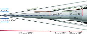

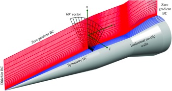

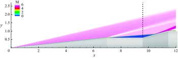


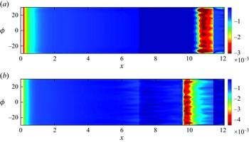


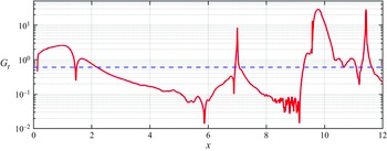


 Open access

