


I. Introduction
A large body of literature documents that investors are inclined to sell assets that have gained in value too early and keep assets that have lost in value for too long. This inclination, known as the disposition effect (DP hereafter, Shefrin and Statman (Reference Shefrin and Statman1985)), plays a prominent role in behavioral finance and behavioral economics literature. The disposition effect has been observed in individual investors (e.g., Odean (Reference Odean1998), Grinblatt and Keloharju (Reference Grinblatt and Keloharju2001), and Feng and Seasholes (Reference Feng and Seasholes2005)), mutual fund managers (Frazzini (Reference Frazzini2006)), investors involved in IPOs (Kaustia (Reference Kaustia2004)), real estate investors (Genesove and Mayer (Reference Genesove and Mayer2001)), and investors in the betting market (Andrikogiannopoulou and Papakonstantinou (Reference Andrikogiannopoulou and Papakonstantinou2020)).
The extant literature has offered several explanations for DP. The most prevalent explanation rests on reference-dependent risk attitudes in prospect theory (Kahneman and Tversky (Reference Kahneman and Tversky1979), Tversky and Kahneman (Reference Tversky and Kahneman1992)). Prospect theory postulates that investors use the purchase price as a reference point, and they become risk-seeking when the asset’s value falls below it and risk-averse when the asset’s value rises above it. As a result, investors are more inclined to sell after a gain and reluctant to sell at a loss (e.g., Shefrin and Statman (Reference Shefrin and Statman1985)). However, this explanation, while intuitive, faces several significant challenges. First, for individuals to show DP, the required degree of risk-seekingness in the loss domain has to be much stronger than the level typically observed in empirical studies (Hens and Vlcek (Reference Hens and Vlcek2011), Barberis (Reference Barberis2013)). Therefore, additional assumptions—such as non-rational time preferences (Barberis and Xiong (Reference Barberis and Xiong2012)) or distinct preferences over realized gains and losses (Barberis and Xiong (Reference Barberis and Xiong2009))—have to be made. Second, empirical studies using prospect theory to explain DP face two serious confounds that are difficult to control for: i) irrational beliefs (Andreassen (Reference Andreassen1988), Weber and Camerer (Reference Weber and Camerer1998), and Maier and Fischer (Reference Maier and Fischer2021)) and ii) non-neutral attitudes toward uncertainty in stock markets (Dimmock, Kouwenberg, Mitchell, and Peijnenburg (Reference Dimmock, Kouwenberg, Mitchell and Peijnenburg2015)).
-
i) One form of irrational beliefs posits that investors may update insufficiently in light of recent signals. Investors may struggle to compute an updated Bayesian posterior belief about what a signal means for the expected value of their asset. Instead of making purely random errors (white noise around a difficult-to-compute, true posterior), investors may exhibit a bias in their belief updating process that results in behavior akin to DP. In doing so, investors could underweight new information (e.g., Enke and Graeber (Reference Enke and Graeber2023)), anchor on the initial prior (Hogarth and Einhorn (Reference Hogarth and Einhorn1992)), and/or suffer from the gambler’s fallacy (Clotfelter and Cook (Reference Clotfelter and Cook1993)). Investors may also (partially) use the mean reversion heuristic (e.g., Odean (Reference Odean1998), Weber and Camerer (Reference Weber and Camerer1998)). All these non-Bayesian belief updating mechanisms can lead to DP without investors having reference-dependent risk attitudes.
-
ii) Numerous studies have shown that people are not only sensitive to objectively quantifiable risk, but also sensitive to uncertainty that is not objectively known, often called “ambiguity” (see, e.g., Trautmann and van de Kuilen (Reference Trautmann, van De Kuilen, Keren and Wu2015a) for a review of the literature).Footnote 1 The probability distribution of asset returns in financial markets is rarely objectively known to investors. Therefore, their attitude toward ambiguity may also drive DP. Individuals are typically ambiguity-averse in the gain domain (Ellsberg (Reference Ellsberg1961)) and ambiguity-seeking in the loss domain (e.g., Wakker (Reference Wakker2010)). If investors use the purchase price as a reference, they will exhibit the tendency to sell assets that have gained in value too early (ambiguity-averse) and keep assets that have lost in value too long (ambiguity-seeking), that is, DP, analogous to the mechanism described by prospect theory. Reference-dependent ambiguity attitudes can explain DP either independently or in combination with reference-dependent risk attitudes.Footnote 2 However, despite its potential importance, the role of ambiguity attitudes in explaining DP has not yet been studied empirically.
Importantly, the mechanism in ii) can be extended to attitudes toward second-order uncertainty, beyond just ambiguity. While first-order risk concerns the probability of an outcome given a known return generating process (e.g., the likelihood of a coin landing on heads given the coin’s quality), second-order uncertainty relates to the probability distribution about different return generating processes (e.g., the probability that the coin is fair). Ambiguity describes a situation where the probability of different return generating processes is truly unknown due to investors’ lack of experience and information. However, when investors have conducted in-depth research and accumulated extensive experience, the probability distribution of different return-generating processes may be perceived as objectively known, which is referred to as “compound risk.” Both forms of second-order uncertainty—attitudes toward truly unknown probabilities (ambiguity) and attitudes toward objectively known probabilities (compound risk)—may significantly influence behavior, yet existing research remains inconclusive about how these two forms differ in their effects (Halevy (Reference Halevy2007), Gillen, Snowberg, and Yariv (Reference Gillen, Snowberg and Yariv2019), and Wu, Fehr, Hofland, and Schonger (Reference Wu, Fehr, Hofland and Schonger2024)), particularly in relation to their impact on the disposition effect among financial professionals.
To measure and disentangle the behavioral drivers of DP mentioned above, we design a theory-driven, lab-in-the-field experiment that allows us to detect DP at the individual level and separately identify investors’ beliefs, first-order risk attitudes, and second-order uncertainty attitudes (including ambiguity). This method allows us to gain, on the one hand, control over the variables of interest, and, on the other hand, some external validity by administering the experiment to financial professionals with substantial business experience.
In the experiment, financial professionals hold a financial asset that follows a stochastic process along a binomial tree for two periods. The specific asset they hold can be of two types, where the GOOD type has a higher (objectively known) probability of increasing in value per period than the BAD type. Importantly, investors do not know which type of asset they hold. In two treatments, we vary whether the probability of having a GOOD or a BAD asset is objectively known (in the RISK treatment) or not (in the AMBIGUITY treatment). As a result, the financial professionals face a rich environment with multiple levels of uncertainty, as in real financial markets: a first-order risk about how the value of the asset develops in the next period (increase or decrease) conditional on the type of the asset, and a second-order uncertainty about the likelihood that the type of asset they hold is GOOD or BAD.
After one period in the binomial tree, we elicit from each financial professional, conditional on the performance of their asset in the first period: i) the certainty equivalent value of their asset, ii) the two matching probabilities that their asset’s value is increasing (decreasing) in the next period, and iii) their willingness to sell the asset at the Bayesian (risk-neutral) value. Participants’ behavior in these decisions is governed by a combination of beliefs (regarding the type of asset they hold) and attitudes toward first-order risk as well as second-order uncertainty. The latter, by design, includes attitudes toward ambiguity in the AMBIGUITY treatment and attitudes toward compound risk in the RISK treatment. We show that, since one payment option in the elicitation of matching probabilities involves risky lotteries and the other involves ambiguity or compound risk, the matching probabilities may be distorted and do not directly reflect participants’ beliefs. Using the Smooth (ambiguity) model of Klibanoff, Marinacci, and Mukerji (Reference Klibanoff, Marinacci and Mukerji2005) and Seo (Reference Seo2009), we then identify beliefs, risk attitudes, ambiguity attitudes (and, more generally, second-order uncertainty attitudes) from participants’ experimental decisions and quantify their relative importance in explaining observed selling behavior that is congruent with DP.Footnote 3
The experimental results show that a substantial proportion of professionals in our sample exhibited DP: 34% of 237 participants were willing to sell their asset after a gain but not after a loss. Individual-level decomposition analyses indicate that, while participants were generally more risk-averse in the UP scenario than in the DOWN scenario, only 19% of those exhibiting DP were risk-averse in the UP scenario and risk-seeking in the DOWN scenario. Similarly, only 7% of participants with DP showed aversion to second-order uncertainty (compound risk or ambiguity) in the UP scenario and seeking toward it in the DOWN scenario. In contrast, participants’ elicited beliefs were non-Bayesian, because participants did not sufficiently update their beliefs in response to new information relative to the Bayesian benchmark. This non-Bayesian updating resulted in an underestimation (overestimation) of future value increases (decreases) and in trading behavior consistent with DP. Multinomial regressions assessing the relative importance of different determinants provide further support for this interpretation, suggesting that DP is driven less by reference-dependent attitudes toward risk or second-order uncertainty and more by irrational beliefs.
Our study complements the burgeoning literature explaining DP using empirical or simulated data (Barberis and Xiong (Reference Barberis and Xiong2009), Kaustia (Reference Kaustia2010), and Ben-David and Hirshleifer (Reference Ben-David and Hirshleifer2012), among others). By eliciting variables typically not observable in market data using a controlled experiment, our article extends the scope of the empirical literature on DP in three important directions.
-
i) As explained above, there is an extensive debate about whether DP is driven by attitudes toward risk and uncertainty (e.g., Shefrin and Statman (Reference Shefrin and Statman1985), Dimmock, Kouwenberg, Mitchell, and Peijnenburg (Reference Dimmock, Kouwenberg, Mitchell and Peijnenburg2015)) or beliefs (e.g., Weber and Camerer (Reference Weber and Camerer1998), Corneille et al. (Reference Corneille, De Winne and D’hondt2018)). We contribute to this discussion by offering a novel design that separately identifies the role of attitudes toward risk and second-order uncertainty (“tastes”) and beliefs. Note that participants’ matching probabilities may not directly reflect their beliefs, because they can be distorted by non-neutral attitudes toward second-order uncertainty. In our design, we are able to measure beliefs from matching probabilities, controlling for attitudes toward second-order uncertainty by using the Smooth model (Klibanoff et al. (Reference Klibanoff, Marinacci and Mukerji2005), Seo (Reference Seo2009)). Our results contribute to the ongoing debate by providing evidence in favor of the view that DP is driven primarily by non-Bayesian beliefs and less so by attitudes toward risk and second-order uncertainty.
-
ii) Our experimental design allows us to test whether participants exhibit a disposition effect at the individual level, rather than analyzing general trading patterns (see, e.g., Odean (Reference Odean1998)). This approach helps to assess theoretical predictions based on individual attitudes. For instance, based on our experimental data, financial professionals are not more likely to fall prey to DP when they are averse (seeking) toward risk or second-order uncertainty after the value of their asset increased (decreased). This is in line with our interpretation that irrational beliefs, rather than reference-dependent risk or uncertainty attitudes, are the primary driver of DP.
-
iii) Previous experimental studies on DP used students as participants (e.g., Andreassen (Reference Andreassen1988), Weber and Camerer (Reference Weber and Camerer1998)). Studying DP with financial professionals is important, given that finance theory typically assumes that prices are determined by the trading behavior of presumably rational investors. In line with this, evidence suggests that more sophisticated investors are less prone to decision errors and thus perform better (e.g., Noussair, Tucker, and Xu (Reference Noussair, Tucker and Xu2016), Corgnet, Desantis, and Porter (Reference Corgnet, Desantis and Porter2018), and Kirchler, Lindner, and Weitzel (Reference Kirchler, Lindner and Weitzel2018)). Feng and Seasholes (Reference Feng and Seasholes2005) and Dhar and Zhu (Reference Dhar and Zhu2006) posit that DP may diminish with experience. Shapira and Venezia (Reference Shapira and Venezia2001) conclude that independent investors are more prone to DP than investors whose accounts are managed by a brokerage professional, even though both types of investors exhibit DP.Footnote 4 Our experimental results suggest that a significant portion of our sample of financial professionals (34%) is prone to DP. Moreover, we find that financial professionals with longer working experience, or those working as traders, do not seem to exhibit lower levels of DP.
The remainder of this article is organized as follows: Section II describes the experimental design and implementation. In Section III, we present the results. Section IV concludes the article and discusses its implications.
II. Experimental Design
A. Basic Setup and Treatments
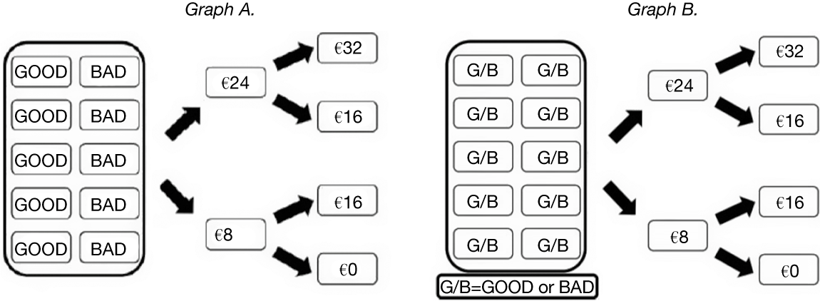
At the start of the experiment, all participants were endowed with an asset with an initial value of €16. As shown in Figure 1, the value of the asset followed a random walk along a binomial tree for two periods, increasing or decreasing by €8 per period. Consequently, after two periods, the redemption value of the asset was €32, €16, or €0. Only the final redemption value after two periods (i.e., at the end of the experiment) was payoff relevant. Therefore, the intermediate values of €24 and €8 in Figure 1 only indicate the pathway the asset value might take, but did not lead to a payout after the first period.
Figure 1 illustrates the potential development of the value of the asset over two periods after an initial random draw of the type of the asset (GOOD or BAD) in the RISK treatment (Graph A) and the AMBIGUITY treatment (Graph B).

Participants did not know which type of asset they held, which could be either GOOD or BAD. The GOOD type had an objectively known probability of ¾ to increase (¼ to decrease) in value per period, while the respective probabilities for the BAD type were ¼ (increase) and ¾ (decrease).
In the RISK treatment, the probability of having a GOOD or BAD asset was objectively known and equal to 0.5. Specifically, participants knew that the type of their asset was determined by a random draw from an urn with 10 assets consisting of exactly 5 GOOD assets and 5 BAD assets.
In the AMBIGUITY treatment, the type of their asset was determined by a random draw from an urn with 10 assets with an unknown proportion of GOOD and BAD assets. In other words, the probability of getting an asset of a certain type was unknown to participants, which is common in experiments on ambiguity (e.g., Halevy (Reference Halevy2007)).
Hence, participants faced two orders of uncertainty about the asset. The first-order uncertainty is the probability of the change of the asset’s value conditional on the type of the asset. This uncertainty is about risk in both treatments since there exists an objective payoff distribution for each type of asset: increase with a probability of ¾ for the GOOD asset and ¼ for the BAD asset (decrease otherwise). The second-order uncertainty is about the likelihood that the asset is of the type GOOD or BAD. This second-order uncertainty involves unknown probabilities in the AMBIGUITY treatment and compound risk in the RISK treatment. The treatments were administered between-subjects, that is, each financial professional participated either only in the RISK treatment or only in the AMBIGUITY treatment.
B. Decisions in Two Scenarios
In the experiment, we asked participants to make four decisions in each of two scenarios: UP and DOWN. In the UP scenario, participants were asked to make decisions conditional on the event that the value of their asset had increased to €24 in the first period. Thus, in the last period, the asset would have a payoff-relevant redemption value of either €32 or €16. Analogously, in the DOWN scenario, participants made decisions conditional on a decrease of their asset’s value to €8 in the first period, with a final redemption value of €16 or €0. In this sense, we implemented the so-called strategy method, because participants first made decisions conditional on each possible scenario of the real choice environment, and then the actual realization was randomly determined (and communicated) at the end of the experiment to determine the payoffs. All participants were placed into the two scenarios sequentially, but we randomized the order of the scenarios to control for potential order effects.
1. Decision 1: Certainty Equivalent
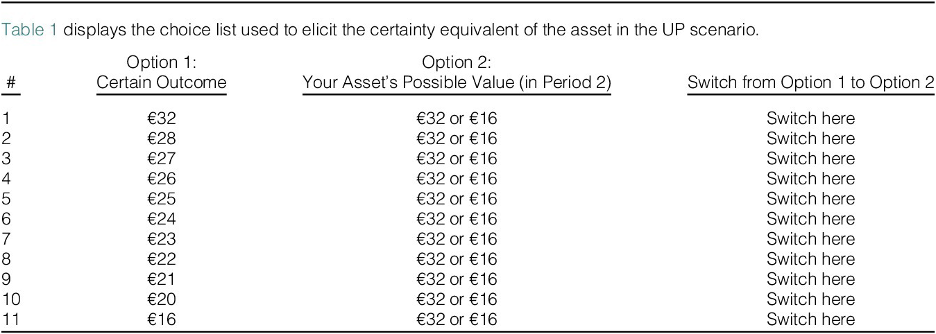
In each scenario (UP and DOWN), we elicited the certainty equivalent of the asset at the end of the first period using a choice list. In this choice list, participants faced a table with 11 rows, each containing a choice between receiving a sure amount and receiving the asset value at the end of the second period. The maximum and minimum of the sure amounts were equal to the maximum and minimum final value of the asset: €32 or €16 in the UP scenario, and €16 or €0 in the DOWN scenario. The sure amount changed in increments of €1, except for the initial and final steps, which involved €4 increments. Table 1 presents the choice list in the UP scenario. To avoid experimental fatigue, we asked participants to click on the row at which they started to prefer the asset over the sure amount. Once participants clicked on this switching row, their preferred option in each row was highlighted in bold and with a larger font size. Participants could change their decision by clicking on a different row before they confirmed their choice and proceeded to the next decision. To help participants better understand the choice list, we also provided a concrete example directly below the choice list to illustrate the potential consequences of their choice.

2. Decisions 2 and 3: Matching Probabilities
In Decision 2, we employed a choice list to elicit participants’ matching probability of a future increase in their asset’s value (see Table 2). Option 1 was a prospect that paid €20 with an objective probability p, and €0 otherwise. Moving down the rows, p varied from 75% (the chance when participants are 100% sure the asset is GOOD) to 25% (the chance when participants are 100% sure the asset is BAD) at increments of 5%. Option 2 was a fixed prospect that paid €20 if the asset’s value increased in the next period, and €0 otherwise. Similar to Decision 1 (about the certainty equivalent), we asked participants to indicate the row at which they started to prefer Option 2 over Option 1. With the switching point, we were eliciting participants’ matching probabilities for an increasing asset value in the next period (see, e.g., Trautmann and van de Kuilen (Reference Trautmann and van de Kuilen2015), (Reference Trautmann and van de Kuilen2015b) and Baillon, Huang, Selim, and Wakker (Reference Baillon, Huang, Selim and Wakker2018)).

Table 2 presents the choice list of Decision 2, where each row represents a choice between a prospect yielding €20 with an objective probability p and a prospect yielding €20 if the value of the asset would increase in the next period. Specifically, we elicited the objective probability that made participants indifferent between receiving the prospect in Option 1 (pINC: €20, 0) and the prospect in Option 2 (EINC: €20, 0), where EINC denotes the event that the value of the asset would increase in the next period.
The choice list for Decision 3 was almost identical to Decision 2, with the only difference being that Option 2 was a fixed prospect that paid €20 if the asset’s value decreased in the next period, and €0 otherwise. Hence, we elicited the matching probability pDEC that made participants indifferent between the prospect (pDEC: €20, 0) and the prospect (EDEC: €20, 0), with EDEC denoting the event that the value of the asset would decrease in the next period.
We administered Decisions 2 and 3 in both the UP and DOWN scenarios. Therefore, in total, we elicited four matching probabilities per participant: two for increasing asset values in scenarios UP and DOWN, and two for decreasing asset values in both scenarios.
3. Decision 4: Selling Against a Fixed Value
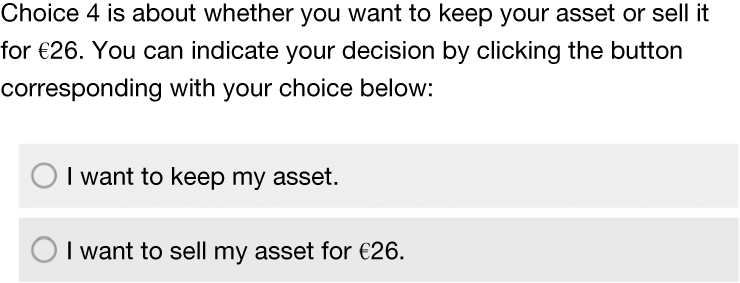
The final decision in each scenario involved a direct choice between keeping the asset for one more period or selling it for €26 in the UP scenario and for €6 in the DOWN scenario, as shown in Figure 2. In the following subsection, we will explain the choice of these two values (€26 in the UP scenario and €6 in the DOWN scenario). For the time being, note that a decision to sell the asset in the UP scenario but to hold it in the DOWN scenario is consistent with DP.
Figure 2 shows the choice given to respondents to keep or sell their asset against the Bayesian value in the UP scenario.

C. Theoretical Analyses and Measurements
In this section, we first theoretically discuss how risk attitudes, attitudes toward second-order uncertainty, and beliefs can lead to DP in our experimental setting. Then, we demonstrate how we measure and isolate these determinants from the experimental data.
In our experimental setting, participants face a two-stage lottery. The first-stage lottery involves the probability of a further change of the asset’s value (+€8 or –€8), conditional on the asset type. Since this probability is objectively known (¾ or ¼), this first-stage lottery is about risk. The second-stage lottery depends on the posterior belief (μ) about the asset being of the type GOOD in each scenario. In the RISK treatment, the prior is 50%, and thus the Bayesian posterior is 75% in the UP scenario and 25% in the DOWN scenario. In the AMBIGUITY treatment, although the prior belief about the asset’s type is unknown, a natural prior is 50% since there is no reason to favor either asset type. This leads to the same posteriors as in the RISK treatment.
Under subjective expected utility theory, participants’ matching probabilities (Decision 2 and 3) about the further change of the asset’s value directly reflect participants’ beliefs. Under Bayesian updating, these beliefs are 62.5% and 37.5% in the UP scenario and 37.5% and 62.5% in the DOWN scenario, respectively.Footnote 5 It follows that participants’ certainty equivalents (Decision 1) in the UP and DOWN scenarios are €26 (=0.625 × 32 + 0.375 × 16) and €6 (=0.375 × 16 + 0.625 × 0) when they are risk-neutral, less than €26 and €6 when they are risk-averse, and greater than €26 and €6 when they are risk-seeking. When deciding whether to sell or keep the asset (Decision 4), participants should be indifferent between selling or keeping the asset when they are risk neutral, and sell (keep) the asset in both scenarios when they are risk-averse (seeking, respectively). Consequently, under Bayesian updating and subjective expected utility theory, it is unlikely to observe a substantial proportion of participants exhibiting DP.
However, in real life, participants (and investors) may struggle to compute the posterior belief, even if all information about the underlying asset pricing process is transparent and they exert their best cognitive efforts. This opens up the possibility that participants, in light of new signals, insufficiently update their beliefs about the quality of the asset they hold. This phenomenon can arise from various mechanisms. For instance, participants may be uncertain about the true impact of a new signal on the posterior belief and, therefore, underweight it during the belief-updating process (e.g., Enke and Graeber (Reference Enke and Graeber2023)). Another mechanism could be conservatism (Edwards (Reference Edwards1968), Hogarth and Einhorn (Reference Hogarth and Einhorn1992), Epley and Gilovich (Reference Epley and Gilovich2006)), where participants (partially) anchor on the initial prior and adjust insufficiently in light of new information due to inertia or caution (de Clippel, Moscariello, Ortoleva, and Rozen (Reference de Clippel, Moscariello, Ortoleva and Rozen2025)). A further possibility is that participants fall prey to the gambler’s fallacy (Clotfelter and Cook (Reference Clotfelter and Cook1993)): In a challenging updating process, participants may give some weight to the mistaken belief that prices cannot keep going up (prices cannot keep going down), even when it is known and, in principle, understood that price changes are random and independent. A related, but distinct belief is mean-reversion (e.g., Odean (Reference Odean1998), Weber and Camerer (Reference Weber and Camerer1998)): Participants may, against better knowledge, allow for the possibility that winners will cool off and losers will rebound to their long-term average (the unconditional prior in our experiment). All of these biases in the belief updating process trigger a behavior where participants keep losers too long and sell winners too early.Footnote 6
Further, participants may deviate from subjective expected utility theory. In the AMBIGUITY treatment, participants face ambiguity, and their valuation of the asset may be affected by their ambiguity attitudes. In the RISK treatment, participants face a compound lottery, and research suggests that attitudes toward compound risk may be similar to (Halevy (Reference Halevy2007), Gillen et al. (Reference Gillen, Snowberg and Yariv2019)) or differ from (Wu et al. (Reference Wu, Fehr, Hofland and Schonger2024)) ambiguity attitudes. When attitudes toward second-order uncertainty are non-neutral, matching probabilities cannot be directly interpreted as beliefs. In addition, participants may have reference-dependent attitudes toward risk and second-order uncertainty: They may be averse in the UP scenario and seeking in the DOWN scenario. Non-Bayesian belief updating and reference-dependent attitudes, in isolation or combination, may lead to participants’ subjective evaluation of the asset lower than €26 in the UP and higher than €6 in the DOWN scenario. Consequently, they exhibit DP.
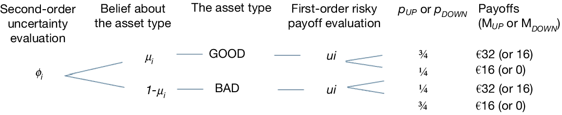
In light of these behavioral tendencies, we follow the Smooth (ambiguity) model (Klibanoff et al. (Reference Klibanoff, Marinacci and Mukerji2005), Seo (Reference Seo2009)) and assume that participants use a utility function ui to evaluate the first-stage risky lottery and a separate function ϕi to evaluate the second-stage lottery, where i = UP or DOWN, implying that u and ϕ can be reference-dependent. Based on the Smooth (ambiguity) model, participants evaluate the asset as follows:
 $$ {\mu}_i{\phi}_i\left[\frac{3}{4}\;{u}_i\left({M}_{INC}\right)+\frac{1}{4}\;{u}_i\left({M}_{DEC}\right)\right]+\left(1-{\mu}_i\right){\phi}_i\left[\frac{1}{4}\;{u}_i\left({M}_{INC}\right)+\frac{3}{4}\;{u}_i\left({M}_{DEC}\right)\right]. $$
where MINC and MDEC are the asset’s possible values in each scenario (MINC = €32 and MDEC = €16 in the UP scenario and MINC = €16 and MDEC = €0 in the DOWN scenario). Figure 3 provides an illustration of this evaluation process.
Figure 3 illustrates the evaluation process of the asset as a two-stage lottery under the Smooth ambiguity model.

In the following, we illustrate how participants’ decisions in the experiment can be used to separately estimate reference-dependent risk attitudes (ui), attitudes toward second-order uncertainty (ϕi), and beliefs ( $ \mu $
i). In the experiment, we elicited two matching probabilities (Decision 2 and 3: pINC and pDEC). Normalizing the utility function so that ui(€20) = 1 and ui(€0) = 0 (€20 and €0 are payoffs in the probability matching decisions), we have
$ \mu $
i). In the experiment, we elicited two matching probabilities (Decision 2 and 3: pINC and pDEC). Normalizing the utility function so that ui(€20) = 1 and ui(€0) = 0 (€20 and €0 are payoffs in the probability matching decisions), we have
 $$ {\displaystyle \begin{array}{c}{\phi}_i\left({p}_{INC}\right)={\mu}_i\;\phi \left(\frac{3}{4}\right)+\left(1-{\mu}_i\right){\phi}_i\left(\frac{1}{4}\right),\\ {}{\phi}_i\left({p}_{DEC}\right)={\mu}_i\;{\phi}_i\left(\frac{1}{4}\right)+\left(1-{\mu}_i\right)\;{\phi}_i\left(\frac{3}{4}\right)\end{array}} $$
Adding both equalities yields the following:
 $$ {\phi}_i\left({p}_{INC}\right)+{\phi}_i\left({p}_{DEC}\right)={\phi}_i\left(\frac{1}{4}\right)+{\phi}_i\left(\frac{3}{4}\right), $$
which is independent of the belief μi. Following Cubitt et al. (Reference Cubitt, van De Kuilen and Mukerji2018), we assume constant relative aversion toward second-order uncertainty (i.e., $ {\phi}_i(x)=1-\left(1+{x}^{\gamma_i}\right)/\left(1-{2}^{\gamma_i}\right) $
). Equation (2) then allows us to identify
$ {\phi}_i(x)=1-\left(1+{x}^{\gamma_i}\right)/\left(1-{2}^{\gamma_i}\right) $
). Equation (2) then allows us to identify $ \gamma $
i for each participant.Footnote
7 For instance, suppose the reported matching probabilities are pINC = pDEC = 0.45 in both scenarios. The coefficient γi then follows from solving 2 × (1 – (1+ 0.45
γ) / (1 – 2
γ)) = (1 – (1+ ¼
γ) / (1 – 2
γ)) + (1 – (1+ ¾
γ) / (1 – 2
γ)), yielding γi ≈ 0.26 in both scenarios, which implies aversion toward second-order uncertainty. In general, sub-additivity (pINC + pDEC < 1) and super-additivity (pINC + pDEC > 1) of the matching probabilities imply second-order uncertainty aversion and seekingness, respectively. Further, the parameter γi can be scenario-specific, for example, aversion to second-order uncertainty in the UP scenario and seeking to second-order uncertainty in the DOWN scenario.
$ \gamma $
i for each participant.Footnote
7 For instance, suppose the reported matching probabilities are pINC = pDEC = 0.45 in both scenarios. The coefficient γi then follows from solving 2 × (1 – (1+ 0.45
γ) / (1 – 2
γ)) = (1 – (1+ ¼
γ) / (1 – 2
γ)) + (1 – (1+ ¾
γ) / (1 – 2
γ)), yielding γi ≈ 0.26 in both scenarios, which implies aversion toward second-order uncertainty. In general, sub-additivity (pINC + pDEC < 1) and super-additivity (pINC + pDEC > 1) of the matching probabilities imply second-order uncertainty aversion and seekingness, respectively. Further, the parameter γi can be scenario-specific, for example, aversion to second-order uncertainty in the UP scenario and seeking to second-order uncertainty in the DOWN scenario.
With the estimated value of $ \gamma $
i, we can use equation (1) to identify μi in the UP and DOWN scenarios. In the example above, since μ
UP = [ϕ
UP(pINC) – ϕ
UP(¼)]/[ϕ
UP(¾) – ϕ
UP(¼)] in the UP scenario, we have μ
UP = [ϕ
UP(0.45) – ϕ
UP(¼)]/[ϕ
UP(¾) – ϕ
UP(¼)] = [(1 – (1+ 0.450.26) / (1–20.26)) – (1 – (1+ ¼0.26) / (1–20.26))] /[(1 – (1+ ¾0.26) / (1–20.26)) – (1 – (1+ ¼0.26) / (1–20.26))] ≈ 0.5 in the UP scenario. A similar calculation shows μ
DOWN ≈ 0.5 in the DOWN scenario.
$ \gamma $
i, we can use equation (1) to identify μi in the UP and DOWN scenarios. In the example above, since μ
UP = [ϕ
UP(pINC) – ϕ
UP(¼)]/[ϕ
UP(¾) – ϕ
UP(¼)] in the UP scenario, we have μ
UP = [ϕ
UP(0.45) – ϕ
UP(¼)]/[ϕ
UP(¾) – ϕ
UP(¼)] = [(1 – (1+ 0.450.26) / (1–20.26)) – (1 – (1+ ¼0.26) / (1–20.26))] /[(1 – (1+ ¾0.26) / (1–20.26)) – (1 – (1+ ¼0.26) / (1–20.26))] ≈ 0.5 in the UP scenario. A similar calculation shows μ
DOWN ≈ 0.5 in the DOWN scenario.
Finally, we assume constant relative aversion for the first-order risk attitude (CRRA): $ {u}_i(x)=1-{\left(1+\frac{x}{20}\right)}^{\alpha_i}/\left(1-{2}^{\alpha_i}\right) $
. With the estimated values of
$ {u}_i(x)=1-{\left(1+\frac{x}{20}\right)}^{\alpha_i}/\left(1-{2}^{\alpha_i}\right) $
. With the estimated values of $ \gamma $
i and μi, the risk attitude parameter
$ \gamma $
i and μi, the risk attitude parameter $ \alpha $
i for the UP and DOWN scenarios can be estimated using the certainty equivalents of the asset in the UP and DOWN scenarios, CE
UP and CE
DOWN (Decision 1), respectively:
$ \alpha $
i for the UP and DOWN scenarios can be estimated using the certainty equivalents of the asset in the UP and DOWN scenarios, CE
UP and CE
DOWN (Decision 1), respectively:
 $$ {\displaystyle \begin{array}{c}\hskip-12em {\phi}_{\mathrm{UP}}\left({u}_{\mathrm{UP}}\left({\mathrm{CE}}_{UP}\right)\right)=\mu\;{\phi}_{\mathrm{UP}}\left(\frac{3}{4}{u}_{\mathrm{UP}}\left(\text{\EUR} 32\right)+\frac{1}{4}{u}_{\mathrm{UP}}\left(\text{\EUR} 16\right)\right)\\ {}\hskip5em +\left(1-\mu \right)\;{\phi}_{\mathrm{UP}}\left(\frac{1}{4}{u}_{\mathrm{UP}}\left(\text{\EUR} 32\right)+\frac{3}{4}{u}_{\mathrm{UP}}\left(\text{\EUR} 16\right)\right)\\ {}\hskip-.2em {\phi}_{\mathrm{DOWN}}\left({u}_{\mathrm{DOWN}}\left({\mathrm{CE}}_{DOWN}\right)\right)=\mu\;{\phi}_{\mathrm{DOWN}}(\frac{3}{4}{u}_{\mathrm{DOWN}}(\text{\EUR} 16)+\frac{1}{4}{u}_{\mathrm{DOWN}}(\text{\EUR} 0))\\ {}\hskip12em +\left(1-\mu \right)\;{\phi}_{\mathrm{DOWN}}(\frac{1}{4}{u}_{\mathrm{DOWN}}(\text{\EUR} 16)\\ {}\hskip2em +\frac{3}{4}{u}_{\mathrm{DOWN}}(\text{\EUR} 0))\end{array}} $$
To continue the above example, suppose the reported certainty equivalent is €20 in the UP scenario and €8 in the DOWN scenario. The CRRA coefficient αi then can be found by solving $ \phi $
UP(u
UP(€20)) = 0.5×
$ \phi $
UP(u
UP(€20)) = 0.5× $ \phi $
UP(¾u
UP(€32) + ¼u
UP(€16)) + 0.5
$ \phi $
UP(¾u
UP(€32) + ¼u
UP(€16)) + 0.5 $ \phi $
UP(¼u
UP(€32) + ¾u
UP(€16)) and
$ \phi $
UP(¼u
UP(€32) + ¾u
UP(€16)) and $ \phi $
DOWN(u
DOWN(€8)) = 0.5×
$ \phi $
DOWN(u
DOWN(€8)) = 0.5× $ \phi $
DOWN(¾u
DOWN(€16) + ¼u
DOWN(€0)) + 0.5
$ \phi $
DOWN(¾u
DOWN(€16) + ¼u
DOWN(€0)) + 0.5 $ \phi $
DOWN(¼u
DOWN(€16) + ¾u
DOWN(€0)) (i.e., α
UP ≈ 0.43 and α
DOWN ≈ 1.02).
$ \phi $
DOWN(¼u
DOWN(€16) + ¾u
DOWN(€0)) (i.e., α
UP ≈ 0.43 and α
DOWN ≈ 1.02).
By linking participants’ Decision 4 to reference-dependent risk attitudes (ui), attitudes toward second-order uncertainty (ϕi), and beliefs ( $ \mu $
i), as identified above, we can assess the relative importance and robustness of these factors in DP, not only at the individual level across treatments but also within and across subgroups.
$ \mu $
i), as identified above, we can assess the relative importance and robustness of these factors in DP, not only at the individual level across treatments but also within and across subgroups.
D. Implementation
The artefactual field experiment was conducted in the Behavioral Finance Online Research (BEFORE) panel (https://before.world/). The panel contains financial professionals from around the world. Several researchers have used this panel to run incentivized economic and financial experiments (see, e.g., Razen, Kirchler, and Weitzel (Reference Razen, Kirchler and Weitzel2020), and Weitzel and Kirchler (Reference Weitzel and Kirchler2023)). In total, 324 respondents participated in our experiment, and 247 respondents completed the experiment. 137 financial professionals were randomly allocated to the RISK treatment, and 110 financial professionals were allocated to the AMBIGUITY treatment.
The experiment was administered between February 24 and March 7, 2021.Footnote 8 Participants received an invitation to participate in the experiment on February 24 and received a reminder on March 1. After reading the experimental introduction, participants answered a control question about the conditional probability of the asset type on the previous increase in the asset’s value. All participants were able to proceed, regardless of whether they answered the control question correctly. At the end of the experiment, we conducted a short survey, eliciting participants’ demographic information such as gender and age. We further asked for their comprehension of the experiment on five scales ranging from (1) “Easy to understand” to (5) “Very confusing, I could not understand any of the questions.” In the analysis of the results, we use the participants’ answers to the control question as well as their responses to the comprehension question as a filter to control for noise in the experiment.
For the experimental payment, one decision was randomly chosen by a computer program for each participant. Randomly selecting one choice for payment (also known as the random incentive mechanism) is a prevalent incentive system in experimental studies (Starmer and Sugden (Reference Starmer and Sugden1991), Myagkov and Plott (Reference Myagkov and Plott1997), and Lee (Reference Lee2008)). It avoids income effects (such as Thaler and Johnson’s (Reference Thaler and Johnson1990) house-money effect) and other potential confounds such as hedging across experimental tasks (e.g., Blanco, Engelmann, Koch, and Normann (Reference Blanco, Engelmann, Koch and Normann2010), Johnson, Baillon, Bleichrodt, Li, van Dolder, and Wakker (Reference Johnson, Baillon, Bleichrodt, Li, van Dolder and Wakker2021)).Footnote 9 If participants received the sure payment, they simply received that amount. If participants received the asset or a prospect, a second random draw determined the outcome of the asset or the prospect. Participants received the payment via a bank transfer. The median survey time was about 15 minutes. The average payment was €11, which translates into an hourly wage of €44.
III. Results
A. Prevalence of the Disposition Effect
Table 3 reports participant demographics in the full sample and across treatments. Our participants are predominantly male (89%), which is consistent with the gender ratio in the financial industry (Boorstin (Reference Boorstin2018), Deloitte (2022)). Most participants reported a good understanding of the experiment (78% rated their understanding as level 1 or 2) and answered the control question correctly (81%). Appendix A provides the list of all variables and their definition used in reporting the results. Table A1 in Appendix A reports the summary statistics of all variables. We do not find systematic differences in the demographics and comprehension of participants between the AMBIGUITY treatment and the RISK treatment.

The disposition effect refers to investors’ tendency to sell assets that have increased in value and to keep assets that have decreased in value. In the experiment, we directly asked participants whether they were willing to sell the asset at the Bayesian value or keep it at the end of the UP and DOWN scenarios (see Decision 4 in Section II.B). These two decisions allow us to directly test for the existence of DP in our sample of financial professionals. Table 4 summarizes the percentage of participants with behavior in line (not in line) with DP and their differences across treatments and samples. Those who were willing to sell the asset for its Bayesian value in the UP scenario but not in the DOWN scenario are referred to as the DP subgroup. Some participants exhibited the opposite of DP (OPDP hereafter): They were willing to sell the asset for its Bayesian value in the DOWN scenario but not in the UP scenario.

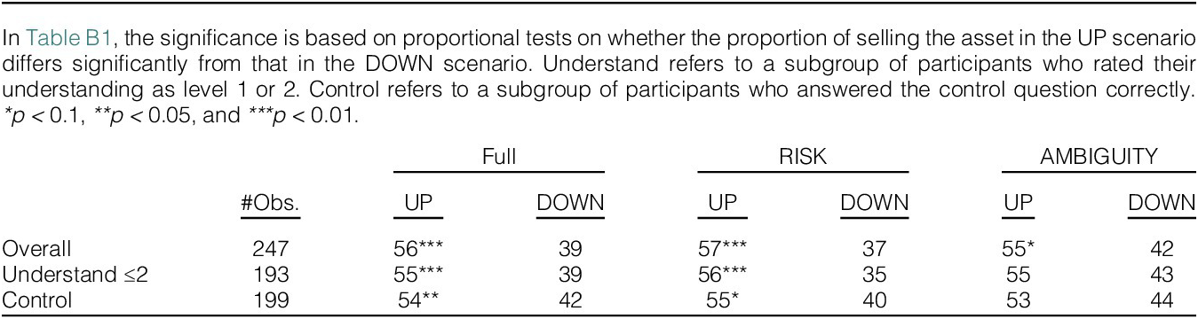
As we can see from Table 4, a substantial proportion of financial professionals exhibited DP, as defined in our task, and consistent with the existing literature. In the full sample, 34% of the 247 participants showed behavior that was consistent with DP. This level is comparable to Cici (Reference Cici2012), who estimated that 22% to 55% of American mutual fund managers tend to realize gains more readily than losses. Meanwhile, 17% of participants exhibited behavior consistent with OPDP. A 2-sided proportional test suggests that the difference is statistically significant (p < 0.01). These values are stable when we look at participants who have a good understanding of the survey or who answered the control question correctly, suggesting that noise or confusion is probably not a driving force behind the participants’ behavior. When looking at each treatment separately, a substantial proportion of financial professionals exhibited DP in both the RISK treatment (34% of 137 participants) and the AMBIGUITY treatment (35% of 110 participants), and a non-negligible proportion of financial professionals exhibited OPDP in both treatments. Table B1 in Appendix B suggests that the percentage of participants who were willing to sell the asset in the UP scenario is significantly higher than that in the DOWN scenario, corroborating the above results.
Given that a substantial proportion of our financial professionals exhibit behavior in line with DP, we can examine whether their observed selling decisions are consistent with their experimentally elicited certainty equivalents (CEs) and matching probabilities.
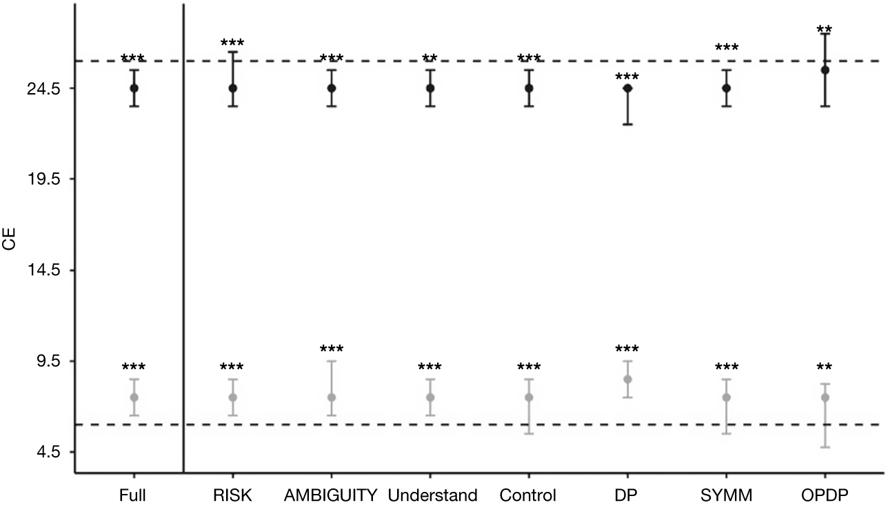
We first compare participants’ CEs for the asset in the UP and DOWN scenarios. Figure 4 reports the 25th, 50th, and 75th percentiles of CEs by scenario, across treatments, and within different subsamples. Consistent with DP, the CEs in the UP scenario are significantly lower than the Bayesian value of €26, while those in the DOWN scenario are significantly higher than the Bayesian value of €6. This pattern holds in the full sample, in the RISK and AMBIGUITY treatments separately, and across subsamples (Wilcoxon signed rank tests, p < 0.01 for all comparisons).
The black and gray lines and dots in Figure 4 denote the 25th, 50th, and 75th percentiles of CE in the UP and DOWN scenarios, respectively. The dashed lines represent the Bayesian value of €26 in the UP scenario and €6 in the DOWN scenario, respectively. Full is the full sample, pooling the RISK and AMBIGUITY treatments. RISK and AMBIGUITY refer to the subgroups of participants in the two treatments. Understand refers to a subgroup of participants who rated their understanding as level 1 or 2. Control refers to a subgroup of participants who answered the control question correctly. DP (OPDP) indicates the subgroup of participants who displayed a disposition effect (its opposite) in their willingness to sell the asset. SYMM indicates the subgroup of participants who behaved symmetrically by either selling or holding the asset in both scenarios. Differences of the median certainty equivalents from the Bayesian benchmark of €26 and €6 are indicated by *p < 0.1, **p < 0.05, and ***p < 0.01, 2-sided Wilcoxon signed rank tests.

Furthermore, participants in the DP subgroup had significantly lower (higher) CEs in the UP (DOWN) than those in the OPDP subgroup (2-sided Wilcoxon tests, p < 0.05 in the UP scenario and p < 0.01 in the DOWN scenario). For comparison, we identified a subgroup, SYMM, consisting of participants who behaved symmetrically by either selling or holding the asset in both scenarios. The certainty equivalents (CEs) of this subgroup fell between those of the DP and OPDP subgroups. The difference in CEs was significant between DP and SYMM (2-sided Wilcoxon tests, p < 0.01 in both scenarios) but not between SYMM and OPDP (2-sided Wilcoxon test, p > 0.10 in both scenarios). We do not find a significant difference in the CEs between the RISK and AMBIGUITY treatments (2-sided Wilcoxon tests, p > 0.10 for both scenarios). More details and comparisons can be found in Table B3 in Appendix B.
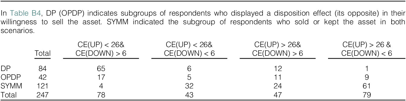
Participants’ observed choices in the experiment could partly be noise (stochastic), affecting our measures of DP (or its opposite). This is particularly relevant since we did not offer an “indifferent” option or conduct repeated measures to reduce measurement error (Gillen et al. (Reference Gillen, Snowberg and Yariv2019)). To investigate this issue, we combined participants’ selling decisions with their CEs to examine the subgroups of DP and OPDP more robustly. CEs would be consistent with DP when they are less than €26 in the UP scenario and greater than €6 in the DOWN scenario (and consistent with OPDP when they are greater than €26 in the UP scenario and less than €6 in the DOWN scenario). We find that, among participants who exhibited DP, 77% had CEs consistent with this effect, while only 1% had CEs consistent with OPDP. In contrast, among those who exhibited OPDP, only 21% had CEs consistent with this effect, whereas 40% had CEs consistent with DP. Using this combined measure (CEs to be consistent with selling decisions), we find that 26% (n = 65) of participants displayed DP, while only 4% (n = 9) were consistent with OPDP. Table B4 in Appendix B provides more details. These results suggest that i) a substantial proportion of participants exhibited DP, even after accounting for their stochastic behavior, and ii) the decisions of participants who displayed OPDP were more stochastic than those displaying DP.
Another approach to link certainty equivalents to DP is to construct composite measures that capture the CEs’ downward deviation from €26 and the upward deviation from €6. Here, we constructed two measures. The first measure is calculated as CDPABS = 26 – CEUP + CEDOWN – 6, where CEUP and CEDOWN stand for certainty equivalents in the UP and DOWN scenarios, respectively, and CDP stands for Composite Disposition Effect. The second measure is relative and calculated as CDPREL = (26 – CEUP)/26 + (CEDOWN – 6)/6. The difference between the two measures is similar to that between the absolute and the relative measure of risk attitudes. In both measures, a positive value implies that participants’ CEs, on average, are less extreme than the Bayesian risk-neutral values, which is consistent with DP. The results show that both measures are significantly positive (Wilcoxon signed rank tests, p < 0.01) in the full sample as well as in each subsample. Further, most participants are consistent with DP according to these two measures (about 78% of participants with CDPABS > 0 and 80% of participants with CDPREL > 0). See Table B2 in Appendix B for more details.
Next, we examine the matching probabilities elicited from Decision 2 and Decision 3 in both the UP and DOWN scenarios, which reflect beliefs about the further movement of the asset’s value. As explained in Section II.C, the matching probabilities in Decision 2 and Decision 3 in each scenario should sum up to 1 if participants are Bayesian and follow subjective expected utility theory. Specifically, the matching probabilities of the asset value increasing further in the UP scenario and decreasing further in the DOWN scenario should each be 62.5%.
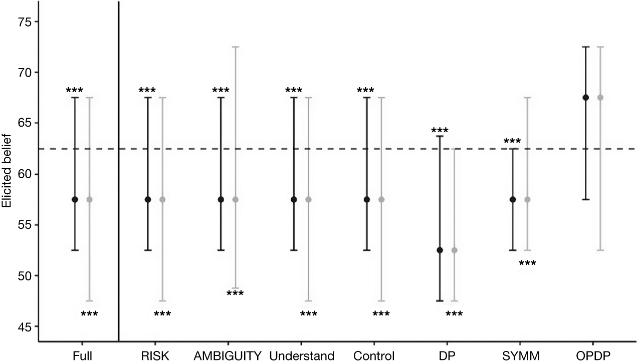
Figure 5 reports the 25th, 50th, and 75th percentiles of the elicited matching probabilities across different scenarios, treatments, and subsamples. Overall, the matching probabilities are strongly biased toward 50% in comparison to the Bayesian posterior (Wilcoxon signed rank test, p < 0.01), suggesting insufficient belief updating: Participants appeared to be too pessimistic in the UP scenario and too optimistic in the DOWN scenario. This result holds in the full sample as well as in the RISK and AMBIGUITY treatments separately (2-sided Wilcoxon signed rank tests, p < 0.01 for all tests). When comparing the matching probabilities of the participants in the DP subgroup versus those in the OPDP group, the former group’s matching probabilities are significantly closer to 50% than those of the latter group, providing further support to the hypothesis of insufficient updating (2-sided Wilcoxon signed rank test, p < 0.01). As with CEs, the matching probabilities of the SYMM subgroup fell between those of the DP and OPDP subgroups. Similar results are observed in subsample analyses, although with slightly weaker significance in some subsamples. For more details, please see Table B5 in Appendix B.
The black and gray lines and dots in Figure 5 denote the 25th, 50th, and 75th percentiles of the matching probabilities in the UP and DOWN scenarios, respectively. The dashed lines represent the Bayesian benchmark of 62.5%. Full is the full sample, pooling the RISK and AMBIGUITY treatments. RISK and AMBIGUITY refer to the subgroups of participants in the two treatments. Understand refers to a subgroup of participants who rated their understanding as level 1 or 2. Control refers to a subgroup of participants who answered the control question correctly. DP (OPDP) indicates the subgroup of participants who displayed a disposition effect (its opposite) in their willingness to sell the asset. SYMM indicates the subgroup of participants who behaved symmetrically by either selling or holding the asset in both scenarios. Differences of the median matching probabilities from the Bayesian benchmark of 62.5% are indicated by *: p < 0.1, **: p < 0.05, and ***: p < 0.01, 2-sided Wilcoxon signed rank tests.

To summarize, the results of the non-parametric analysis suggest a significant disposition effect: A substantial proportion of financial professionals were reluctant to sell a losing asset and more willing to sell a winning asset. Further, their actual selling decisions were consistent with the difference in their CEs and matching probabilities in both scenarios.
However, our results so far cannot distinguish whether the observed disposition effect is due to non-Bayesian beliefs or reference-point dependent attitudes toward risk and second-order uncertainty. Indeed, as we demonstrate in Section II.C, the matching probabilities may not directly capture participants’ beliefs because they can be biased by non-neutral attitudes toward second-order uncertainty. Therefore, at this point, it remains unclear whether the deviations of the matching probabilities and CEs from the Bayesian benchmark are due to insufficient belief updating or due to non-neutral attitudes toward the second-order uncertainty. To examine the exact source of DP, we separately identify these determinants.
B. Decomposing the Determinants of DP
We start by examining whether the change in risk attitude between the UP and DOWN scenarios, as suggested by prospect theory, can account for DP. We then proceed to reference-dependent attitudes toward second-order uncertainty and beliefs. Finally, we evaluate the relative importance of these three determinants in DP.
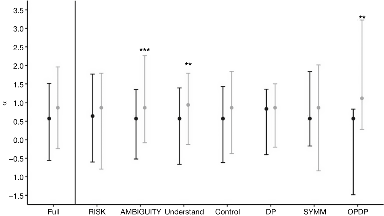
Risk attitudes (α i ) – Figure 6 reports the 25th, 50th, and 75th percentiles of the estimated CRRA coefficient (αi) in both scenarios across treatments using the full and subsamples. The estimated CRRA risk parameter αi in the full sample is significantly lower than 1 in the UP scenario (a median of 0.5964, 2-sided Wilcoxon signed rank test, p < 0.05), indicating risk aversion, while it is not significantly different from 1 in the DOWN scenario (a median of 0.866, 2-sided Wilcoxon signed rank test, p > 0.10). There is some indication that participants were more risk-averse in the UP scenario than in the DOWN scenario. For example, we find a significant difference in the subsample of participants who reported a good understanding of the survey (p < 0.05), in the AMBIGUITY treatment (p < 0.01), and in the subgroup of OPDP participants. See Tables B6 and B7 in Appendix B for more details.
Figure 6 shows the 25th, 50th, and 75th percentiles of the estimated CRRA’s α across treatments and in some subsamples. The black and gray lines denote participants’ risk attitude in the UP and DOWN scenarios, respectively. Full is the full sample. RISK and AMBIGUITY refer to the subgroups of participants in the RISK and AMBIGUITY treatments. Understand refers to a subgroup of participants who rated their understanding as level 1 or 2. Control refers to a subgroup of participants who answered the control question correctly. DP (OPDP) indicates the subgroup of participants who displayed a disposition effect (its opposite) in their willingness to sell the asset. SYMM indicates the subgroup of participants who behaved symmetrically by either selling or holding the asset in both scenarios. Significant differences in median risk attitudes between the UP scenario and the DOWN scenario are indicated by *: p < 0.1, **: p < 0.05, and ***: p < 0.01, 2-sided Wilcoxon signed rank test.

Prospect theory suggests that DP arises from a flip in risk preferences across the two scenarios: risk aversion in the UP scenario and risk-seeking in the DOWN scenario. We thus classify participants’ risk attitudes as risk-averse (α < 0.999), risk-neutral (0.999 < α < 1.001), and risk-seeking (α > 1.001). Since there were no risk-neutral participants, we omit this category in the analysis. We then calculated the proportion of participants exhibiting each pattern of risk attitude in the two scenarios across the three subgroups: DP, SYMM, and OPDP. Table 5 reports the results, which suggest that risk attitudes have limited explanatory power for DP or its opposite. In the DP subgroup, only 19% of participants exhibited risk attitudes consistent with DP, while 29% displayed risk attitudes aligned with the opposite. In contrast, within the OPDP subgroup, just 5% had risk attitudes consistent with OPDP, whereas 54% exhibited risk attitudes in line with DP.

Overall, while participants were more risk-averse in the UP scenario than in the DOWN scenario, analyses based on the individual level suggest that reference-dependent risk attitudes are unlikely to be the main driver of DP.
Attitude toward second-order uncertainty ( $ \gamma $
i
) – The estimated parameter for the attitude toward the second-order uncertainty is significantly larger than 1 in the full sample, in the RISK and AMBIGUITY treatment separately, and in all subsamples (2-sided Wilcoxon tests, p < 0.01 for all tests). The median coefficient of attitudes toward the second-order uncertainty across all participants is 2.2, implying a tendency to seek second-order uncertainty. There is no significant difference in γi between the RISK and AMBIGUITY treatments (2-sided Wilcoxon test, p > 0.10). Similar to the analyses in risk attitudes, we classify participants based on γi as averse (γi < 0.999), neutral (0.999 < γi < 1.001), or seeking (γi > 1.001) in the UP and DOWN scenarios. There are significantly more participants who were seeking second-order uncertainty, rather than being neutral or averse to it (about 60%, on average, and more than 50% in most treatments and subsamples). Comparing attitudes toward the second-order uncertainty between the UP scenario and the DOWN scenario, we do not find a significant difference in most comparisons. These results are consistent with Table B8 in Appendix B, which report the percentage of participants who are averse, neutral, and seeking toward second-order uncertainty across samples and treatments.
$ \gamma $
i
) – The estimated parameter for the attitude toward the second-order uncertainty is significantly larger than 1 in the full sample, in the RISK and AMBIGUITY treatment separately, and in all subsamples (2-sided Wilcoxon tests, p < 0.01 for all tests). The median coefficient of attitudes toward the second-order uncertainty across all participants is 2.2, implying a tendency to seek second-order uncertainty. There is no significant difference in γi between the RISK and AMBIGUITY treatments (2-sided Wilcoxon test, p > 0.10). Similar to the analyses in risk attitudes, we classify participants based on γi as averse (γi < 0.999), neutral (0.999 < γi < 1.001), or seeking (γi > 1.001) in the UP and DOWN scenarios. There are significantly more participants who were seeking second-order uncertainty, rather than being neutral or averse to it (about 60%, on average, and more than 50% in most treatments and subsamples). Comparing attitudes toward the second-order uncertainty between the UP scenario and the DOWN scenario, we do not find a significant difference in most comparisons. These results are consistent with Table B8 in Appendix B, which report the percentage of participants who are averse, neutral, and seeking toward second-order uncertainty across samples and treatments.
Calculating the proportion of participants exhibiting each pattern of attitude toward second-order uncertainty in both scenarios across the three subgroups (DP, SYMM, OPDP), we find that, in the subgroup DP, only 7% were averse in the UP scenario and seeking in the DOWN scenario toward the second-order uncertainty. Similarly, among the OPDP subgroup, only 10% displayed attitudes toward second-order uncertainty consistent with this behavior. This suggests that the change of attitudes toward second-order uncertainty is unlikely to be a primary reason for DP. See Table 6 for more details.

So far, our results indicate that participants’ risk attitudes and attitudes toward second-order uncertainty play a limited role in DP. We now move on to examine the last determinant: participants’ conditional beliefs μ regarding the type of the asset.
Subjective beliefs (μ
i
) – As explained in Section II.C, by estimating and controlling for participants’ attitudes toward second-order uncertainty ( $ \gamma $
i), we obtain a measure of participants’ beliefs that is free of these confounds. We refer to these beliefs as corrected subjective beliefs. Table B9 in Appendix B reports mean corrected subjective beliefs regarding holding the GOOD asset. Figure B1 in Appendix B displays the histogram of the difference between the elicited belief and the corrected belief. The median correction is 5 percentage points. About 45% of participants had a correction of more than 10 percentage points.
$ \gamma $
i), we obtain a measure of participants’ beliefs that is free of these confounds. We refer to these beliefs as corrected subjective beliefs. Table B9 in Appendix B reports mean corrected subjective beliefs regarding holding the GOOD asset. Figure B1 in Appendix B displays the histogram of the difference between the elicited belief and the corrected belief. The median correction is 5 percentage points. About 45% of participants had a correction of more than 10 percentage points.
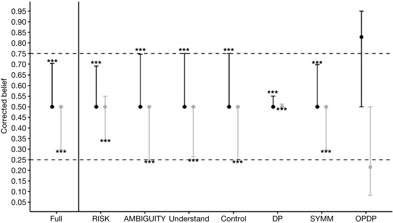
Figure 7 reports the 25th, 50th, and 75th percentiles of the corrected subjective beliefs of holding a GOOD asset, across treatments and scenarios. On average, these beliefs are significantly lower than the Bayesian posterior of 75% in the UP scenario and significantly higher than the Bayesian posterior of 25% in the DOWN scenario, across both treatments and all subsamples (2-sided Wilcoxon tests, p < 0.01 for all comparisons except for the subgroup of OPDP). This indicates that, in both scenarios, participants did not update their beliefs sufficiently in a way consistent with DP.
Figure 7 shows the 25th, 50th, and 75th percentiles of the corrected belief regarding holding the GOOD asset in the UP scenario and in the DOWN scenario, respectively. The black and gray lines denote participants’ beliefs in the UP and DOWN scenarios, respectively. Full is the full sample. RISK and AMBIGUITY refer to the subgroups of participants in the RISK and AMBIGUITY treatments. Understand refers to a subgroup of participants who rated their understanding as level 1 or 2. Control refers to a subgroup of participants who answered the control question correctly. DP (OPDP) indicates the subgroup of participants who displayed a disposition effect (its opposite) in their willingness to sell the asset. SYMM indicates the subgroup of participants who behaved symmetrically by either selling or holding the asset in both scenarios. The significance is about 2-sided Wilcoxon signed rank tests of median against the Bayesian posterior of 75% in the UP scenario and 25% in the DOWN scenario, with *, **, *** denoting the significance level of 10%, 5%, and 1%, respectively.

Finally, we examine the relative importance of risk attitudes, attitudes toward second-order uncertainty, and beliefs in DP via regressions. Since the flip of attitudes between the UP and DOWN scenarios can lead to DP (or its opposite), we constructed two dummy variables for each participant, one based on risk attitudes (α D) and one on attitudes toward second-order uncertainty (γ D). Each dummy equals 1 when the participant flipped attitudes between the two scenarios. For DP (OPDP), this means aversion (seekingness) in the UP scenario and seekingness (aversion) in the DOWN scenario. We also included the difference in the (corrected) beliefs about the asset type being GOOD between the two scenarios ∆μ (= μ DOWN – μ UP), where μ DOWN and μ UP are the (corrected) beliefs in the DOWN and UP scenarios, respectively. The dependent variable is a dummy variable that equals 1 if a participant exhibited DP (or its opposite). Tables B12 and B14 in Appendix B report the results across different samples and treatments. As we can see from these tables, the coefficient for ∆μ is significantly positive (negative) for DP (its opposite, respectively) in all samples and treatments. In contrast, the coefficient for α D has the wrong sign and is statistically significant in some regressions. The coefficient for γ D is not statistically significant in any of the samples or treatments. These regression results are consistent with our earlier findings, suggesting that the behavior of the participants that is consistent with DP (or its opposite) arises predominantly from non-Bayesian beliefs. Tables B13 and B15 in Appendix B report similar analyses with OLS regressions, with qualitatively similar results.
While a shift in attitudes toward risk or second-order uncertainty can contribute to DP or its opposite, such a shift is no longer a necessary condition when combined with beliefs. For instance, even if a participant remains risk-averse in both scenarios, a decrease in risk aversion from the UP scenario to the DOWN scenario could still lead to DP if their attitude toward second-order uncertainty shifts sufficiently from aversion to seeking, and/or if they fail to update their beliefs properly in both scenarios. Taking this into consideration, we conducted a series of multinomial regressions, where the dependent variable has three levels: The base category captures selling or keeping the asset in both scenarios (SYMM); while DP (OPDP) represents trading behavior consistent with (opposite to) DP. The main independent variables are ∆α = α DOWN – α UP: change in risk attitudes between the UP and DOWN scenarios; ∆γ = γ DOWN – γ UP: change in attitudes toward second-order uncertainty between the UP and DOWN scenarios; and ∆μ = μ DOWN – μ UP: difference in (corrected) beliefs about the asset being GOOD between the DOWN scenario and the UP scenario. Reference-dependent attitudes for DP would imply significantly positive coefficients of ∆α and ∆γ, while insufficient updating would suggest a significantly positive coefficient of ∆μ, with the opposite pattern expected for OPDP.
Table 7 reports that the coefficient for ∆μ is consistent with DP (and its opposite) and significant across all samples and treatments. In contrast, the coefficients for ∆α and ∆γ are not significant in any sample or treatment and, in some cases, even have the “wrong” sign. This corroborates our earlier results, which suggest that behavior consistent with DP is primarily driven by non-Bayesian beliefs. Demographic controls such as working experience and the trader dummy do not show any robust relationship with either effect. In Table B14 in Appendix B, we winsorized ∆μ, ∆α, and ∆γ at various thresholds to mitigate the impact of measurement error. The results stayed virtually the same. Table B15 in Appendix B presents regressions that include beliefs in the DOWN and UP scenarios separately, providing further evidence that DP is primarily driven by irrational beliefs.

IV. Conclusion and Discussion
It has been well-documented that investors tend to hold on to losing investments for too long and sell winning investments too quickly. This phenomenon, known as the disposition effect, has been observed both in financial markets and in controlled lab experiments (e.g., Andreassen (Reference Andreassen1988), Odean (Reference Odean1998), Weber and Camerer (Reference Weber and Camerer1998), Genesove and Mayer (Reference Genesove and Mayer2001), and Gneezy (Reference Gneezy2005)). Recognizing that investors in financial markets face uncertainty rather than risk, we motivate our experimental design with the Smooth model (Klibanoff et al. (Reference Klibanoff, Marinacci and Mukerji2005), Seo (Reference Seo2009)), which allows for modelling attitudes toward two orders of uncertainty: one is about risk and the other is about second-order uncertainty (ambiguity or compound risk). By relating decision-makers’ certainty equivalents and matching probabilities for the further movement of the asset’s value to their selling decisions, we are able to decompose the determinants of DP into risk attitude, attitudes toward second-order uncertainty, and beliefs on the individual level.
Our experimental results show that a substantial proportion of financial professionals exhibited behavior that is in line with DP, mirroring the extant literature on the disposition effect using student samples (e.g., Weber and Camerer (Reference Weber and Camerer1998), Jiao (Reference Jiao2017)). We further observe that the elicited matching probabilities did not directly reflect participants’ beliefs because they were distorted by participants’ attitudes toward second-order uncertainty. Most importantly, we provide evidence suggesting that the main determinant of DP, after correcting for attitudes toward risk and second-order uncertainty, is insufficient belief updating in light of new information.
Non-Bayesian belief updating. Our experimental results point toward non-Bayesian belief updating, instead of reference-dependent attitudes toward risk or second-order uncertainty, as the main driver for DP. Such non-Bayesian belief updating could arise from various mechanisms, such as cognitive uncertainty (e.g., Enke and Graeber (Reference Enke and Graeber2023)), the gambler’s fallacy (Clotfelter and Cook (Reference Clotfelter and Cook1993)), or the mean reversion heuristic (e.g., Odean (Reference Odean1998), Weber and Camerer (Reference Weber and Camerer1998)). These mechanisms, individually or jointly, may induce insufficient updating, the underlying drivers of which future research may seek to uncover. For example, one could ask participants about their confidence in their updated beliefs. This would help to differentiate between cognitive uncertainty, where participants lack full confidence in interpreting signals and thus insufficiently incorporate them in their updating, and the gambler’s fallacy or beliefs in mean reversion where participants are convinced that future return developments exhibit specific patterns.
Ambiguity seeking. The majority of finance professionals in our sample are ambiguity-seeking in both scenarios. In the UP scenario, where the asset value increased, it contradicts the common finding of ambiguity aversion (Ellsberg (Reference Ellsberg1961)). A possible explanation is that attitudes toward uncertainty depend on the source that generates the uncertainty (Fox and Tversky (Reference Fox and Tversky1998), Kilka and Weber (Reference Kilka and Weber2001), Abdellaoui, Baillon, Placido, and Wakker (Reference Abdellaoui, Baillon, Placido and Wakker2011), and Baillon, Bleichrodt, Li, and Wakker (Reference Baillon, Bleichrodt, Li and Wakker2025)). For example, Abdellaoui et al. ((Reference Abdellaoui, Baillon, Placido and Wakker2011), Figure 9) observe that French students prefer to bet on uncertainty events generated by the temperature in Paris, rather than on uncertainty events generated by the performance of the French stock index, controlling for the likelihood of the uncertain events. This source preference can accommodate the home bias in finance (Abdellaoui et al. (Reference Abdellaoui, Baillon, Placido and Wakker2011)). Consistent with the source theory of ambiguity, finance professionals display a seeking attitude toward uncertainty because uncertainty in our experiment is generated by the performance of an asset, about which they may feel more competent and knowledgeable. In that sense, our findings confirm descriptive psychological theories of ambiguity that aim to incorporate such source preference (e.g., Einhorn and Hogarth (Reference Einhorn and Hogarth1985), Tversky and Fox (Reference Tversky and Fox1995)). Further, we did not find any robust differences between the RISK and AMBIGUITY treatments, suggesting that investors may behave similarly toward ambiguity and compound risk.
External validity. Our experimental framework is theory-driven (Klibanoff et al. (Reference Klibanoff, Marinacci and Mukerji2005), Seo (Reference Seo2009)) and carefully controlled, allowing us to separate beliefs from attitudes toward risk as well as second-order uncertainty. However, the asset values in the experiment are exogenously given, instead of endogenously determined by market interactions and beliefs regarding other investors’ behavior. In real financial markets, these factors may significantly contribute to DP. For instance, investors may develop beliefs that a price surge or decline has been excessive due to herding behavior. Motivated by such beliefs, investors will sell an asset after a substantial price increase and hold it after a substantial decline, exhibiting DP. In addition, despite paying more than what one usually pays for a more convenient student sample, the stakes in the experiment are relatively small, which may limit the influence of risk attitudes (e.g., Holt and Laury (Reference Holt and Laury2002), Booij and van de Kuilen (Reference Booij and van de Kuilen2009)). Investigating the role of beliefs and attitudes toward risk as well as second-order uncertainty in DP within real financial markets remains a promising and challenging research direction.
Limitations. Of course, our study does not conclude the topic, but should be seen as another step in the quest to unravel the underlying drivers of the disposition effect. We readily acknowledge that our results and conclusions are based on experimental data that stem from a relatively small sample of participants with a limited number of observations per participant. This limits our inference of preference parameters, which, despite winsorization in robustness checks, might include substantial noise. Moreover, we assume specific functional forms that might not be a correct characterization of participants’ decision-making under uncertainty. Finally, while the controlled experimental environment helps to isolate key mechanisms, it is nevertheless possible that our null results with respect to reference-dependent risk and uncertainty aversion/seekingness are due to insufficient power and measurement error. Overall, our conclusions should be interpreted as suggestive and in need of further support by future research.
Appendix A. Key Variables and Summary Statistics
- DP
-
The disposition effect: the tendency to sell the asset for its Bayesian value in the UP scenario but not in the DOWN scenario.
- SYMM
-
The pattern of symmetrically selling or holding the asset in both scenarios.
- OPDP
-
The opposite of the disposition effect: the tendency to sell the asset for its Bayesian value in the DOWN scenario but not in the UP scenario.
- CEUP and CEDOWN
-
The certainty equivalent of the asset in the UP scenario and in the DOWN scenario, respectively.
- CDPABS = 26 – CEUP + CEDOWN – 6
-
A composite measure that captures the certainty equivalents’ downward (upward) deviation from €26 (€6).
- CDPREL = (26 – CEUP)/26 + (CEDOWN – 6)/6
-
A composite measure that captures the certainty equivalents’ relative downward (upward) deviation from €26 (€6).
- p INC, pDEC
-
The matching probability that the asset’s price will increase (decrease) in each scenario, respectively.
-
ui(x) = 1 – (1+ $ \Big(\frac{x}{20} $
)
α)/(1 – 2
α)
$ \Big(\frac{x}{20} $
)
α)/(1 – 2
α) -
The CRRA utility function parameter αi, i = UP or DOWN.
- α UP, α DOWN
-
Estimated risk attitude of CRRA parameter in the UP (DOWN) scenario, respectively.
- α D
-
Dummy variable that equals 1 when a participant was risk-averse in the UP scenario and risk-seeking in the DOWN scenario.
- α O
-
Dummy variable (opposite of α D) that equals 1 when a participant was risk-seeking in the UP scenario and risk-averse in the DOWN scenario.
- ϕi(x) = 1 – (1+ xγ) / (1 – 2 γ)
-
The function that captures the attitude toward the second-order uncertainty with parameter γi, i = UP or DOWN.
- γ UP, γ DOWN
-
Estimated attitude toward the second-order uncertainty in the UP (DOWN), respectively. It refers to the attitude toward compound lottery in the RISK treatment, and to the attitude toward ambiguity in the AMBIGUITY treatment.
- γ D
-
Dummy variable that equals 1 when a participant was averse in the UP scenario and seeking in the DOWN scenario toward second-order uncertainty.
- γ O
-
Dummy variable (opposite of γ D) that equals 1 when a participant was seeking in the UP scenario and averse in the DOWN scenario toward second-order uncertainty.
- μ UP, μ DOWN
-
The belief that the asset is of Type GOOD conditional on being in the UP scenario and in the DOWN scenario, respectively.
- ∆μ = μ DOWN –μ UP
-
The difference of (corrected) beliefs about the asset type being GOOD in the UP scenario and in the DOWN scenario.


Appendix B. Additional Tables


The histogram in Figure B1 shows the difference between the elicited belief and corrected belief regarding the development of the value of the asset.

Supplementary Material
To view supplementary material for this article, please visit http://doi.org/10.1017/S0022109025102159.


 Open access