


1. Introduction
Turbulent jet mixing processes have been a research topic of interest for many years, driven by the many uses of jets in multiple industrial applications. The current work is motivated by engineering design requirements for aerospace propulsion nozzle high-speed exhaust plumes. High-speed jets are characterised by Mach numbers  ${M_j} = {U_j}/{a_j} > \mathrm{\sim }0.7$ (Uj, aj are the jet discharge velocity and speed of sound). This covers the high subsonic and supersonic exhaust flows occurring in civil (Mj ~ 0.7–0.9) and military (Mj ~ 1.0–2.0) aerospace. In both applications it is the jet near field which is of interest – approximately the first 15D of plume development (D = nozzle exit diameter). The far field, where self-similar behaviour has allowed a good understanding of mean flow/turbulence characteristics, is only established some way downstream of this. Near-field flow and turbulence characteristics are considerably more complex than in the far field, but detailed understanding and accurate measurements for validation of prediction methods are crucial to address two specific design challenges.
For civil aeroengines the principal interest is in jet acoustics. Significant progress has been made in reducing engine noise, but jet noise remains a dominant component at take-off, with ever more stringent legislative limits regularly introduced (Flightpath 2050 2011). Peak acoustic source amplitude occurs just downstream of the jet potential core end (Lp), the axial location where the nozzle lip shear layer reaches the jet centreline (typically x/D = 5–10, where x is downstream coordinate). The jet/ambient shear layer from a round nozzle initially resembles a planar shear layer, however, as its inner edge approaches the centreline it is modified into an annular shear layer and the process of merging into a fully formed jet begins downstream of Lp. Thus, the near-field turbulence environment does not correspond to a single, geometrically simple, shear flow type. To optimise noise reduction technologies based on manipulation of jet shear layers (serrations or chevrons, Xia, Tucker & Eastwood Reference Xia, Tucker and Eastwood2009; Callender, Gutmark & Martens Reference Callender, Gutmark and Martens2010), detailed understanding is needed of the near-field shear layer growth rate  $(\delta ^{\prime})$ and its turbulence properties as well as accurate data on Lp and how this varies with jet operating parameters. In military engines, the exhaust system operates at supercritical nozzle pressure ratios (NPR = Pt,j/pa = jet total pressure/ambient static pressure – NPRcrit = 1.89 assuming dry air specific heat ratio γ = const. = 1.4, varying <0.3 % up to ~1300 K). This leads to supersonic jets with embedded shock structures for improperly expanded operating conditions. The principal design challenge for the military application is enhancement of near-field jet/ambient mixing rate via letter-box or bevelled nozzle geometries, internal lobed mixers or tabs/fluidic injection mixing devices. Both applications involve hot jets characterised by the nozzle temperature ratio (NTR = Tt,j/Ta, jet total temperature to ambient static temperature ratio). The static temperature ratio (t = Ts,j/Ta, jet divided by ambient static temperature) is sometimes preferred, with gas dynamics connecting NTR and t (e.g. $NTR = t(1 + (\gamma - 1)/2M_j^2)$ for a fully expanded nozzle). Enhanced mixing enables rapid jet temperature decay, reducing infra-red (IR) signature and improving low observability (Dash et al. Reference Dash, Pearce, PerGament and Fishburne1980; Mahulikar, Sonawane & Rao Reference Mahulikar, Sonawane and Rao2007). The parameter Lp represents a characteristic length scale for the maximum temperature region, and thus accurate knowledge of Lp and technologies to decrease Lp via enhanced shear layer mixing are important design issues.
Near-field jet development is obviously influenced by the presence of the flight stream surrounding the propulsive jet, reducing strain rate and mixing rate and thus increasing Lp and the spatial extent of the near field. Flight stream effects have recently been studied using large eddy simulation (LES) by Naqavi et al. (Reference Naqavi, Wang, Tucker, Mahak and Strange2016). No flow or turbulence measurements were available to confirm the accuracy of simulation results, but comparison with far-field acoustic data was encouraging. However, even the canonical case of a single axisymmetric hot high-speed jet in a stagnant ambient has received only limited experimental study (detailed review in § 2) with little consensus on the effect of heat addition. To aid development of the technologies needed, it is important that a suitable experimental database is available for this baseline flow covering the practically relevant Mj and NTR (or t) range. The present work describes an experimental study focussed on establishing a coherent understanding of the influence of Mj and NTR/t on the principal parameters characterising jet near-field aerodynamics – shear layer spreading rate  $(\delta ^{\prime})$ and potential core length (Lp).
Existing experimental data are reviewed in § 2 and gaps/inconsistencies identified. An experimental study which complements and extends existing measurements has been conducted in an appropriate test facility and with instrumentation outlined in § 3. Section 4 reports and analyses the results, allowing a coherent picture of heat addition effects on  $\delta ^{\prime}$ and Lp for high Mj jets to be identified. Principle conclusions from the work are summarised in § 5.
2. Previous work
2.1. Static density/temperature ratio effect in low-speed shear layers/jets
In incompressible flows, free shear layers are known to be susceptible to instabilities excited by velocity and density ratios across the shear layer (Michalke Reference Michalke1984; Morris Reference Morris2010). Instability waves grow faster when density decreases on the higher-speed side of the shear layer. For a laminar boundary layer at nozzle exit, such instabilities help trigger the transition to turbulence. Even for fully turbulent shear layers they influence the development of the near nozzle large-scale eddies which dominate mixing. The effect of static density ratio  $s = {\rho _2}/{\rho _i}$ across a turbulent shear layer with velocity ratio $r = {U_2}/{U_1}$ has been studied experimentally (using different gases to control s) by Brown & Rosko (Reference Brown and Rosko1974) (subscript 1 is the faster (jet) stream and 2 is the slower (stagnant ambient) stream). Measurements identified the dependence of shear layer width growth rate $(\delta ^{\prime})$ on r and s. Note that, in what follows, although results were expressed in terms of s, to place these in the current hot jet context, they are here presented in terms of static temperature ratio, since: $s = {\rho _a}/{\rho _j} = {T_{s,j}}/{T_a} = t$ (ignoring pressure effects). The vorticity thickness $\delta _{\omega} = ({U_1} - {U_2})/{(\partial U/\partial z)_{max}}$ was used to characterise shear layer width (z is the coordinate across the shear layer) and the growth rate relation was
 \begin{equation}\delta ^{\prime}_\omega = 0.0825\frac{{(1 - r)}}{{(1 + r{t^{1/2}})}}(1 + {t^{1/2}}).\end{equation}
Dimotakis (Reference Dimotakis1986) proposed a modified version of (2.1) taking into account the asymmetric entrainment into the mixing region from high-speed and low-speed sides, although only ~15 % difference to (2.1) resulted and only at extreme values of r and t. For a jet in stagnant surroundings (U 2 = 0, i.e. r = 0) with an expected maximum t of ~3, the difference was only ~6 %. When applied to a hot jet in stagnant surroundings (2.1) indicates shear layer width growth is modified by the square root of jet/ambient static temperature ratio
 \begin{equation}\delta ^{\prime}_\omega = 0.0825(1 + {t^{1/2}}).\end{equation}
This implies a significant although fairly weak effect; the growth rate increases by only 37 % for a static temperature ratio increase of 300 %. The LES study of McMullan, Coats & Gao (Reference McMullan, Coats and Gao2011) did not compare directly with the Brown & Roshko data, but the predicted results may be deduced as in very good agreement with (2.1).
A similar square root density ratio influence on the spreading rate of a variable density jet in stagnant surroundings – this time for the developed jet not just the initial shear layer – had been suggested earlier by Thring & Newby (Reference Thring and Newby1953). These authors introduced the concept of an ‘effective diameter’  $({D_{eff}} = D{({\rho _j}/{\rho _a})^{1/2}})$; when Deff was used as the governing length scale axial decay of measured jet velocity collapsed for all temperature ratios studied (t = 0.196–7.14). Ricou & Spalding (Reference Ricou and Spalding1961) performed direct measurements of entrainment for jets with different density ratios and confirmed this effect. Jet entrainment and centreline velocity decay rate both increased when jet density was less than ambient density but all data collapsed onto a single line when scaled by t 1/2. Other variable density jet experiments have observed a similar relationship (Pitts Reference Pitts1991; Amielh et al. Reference Amielh, Djeridane, Anselmet and Fulachier1996).
2.2. Compressibility effects in high-speed shear layers
The jet studies described above were restricted to low Mach number. However, measurements by Zaman (Reference Zaman1998) showed that a t 1/2 parameter was equally successful in collapsing the downstream asymptotic spreading rate behaviour of compressible jets as long as shock-free conditions existed. The same was not true, however, for the initial shear layer development. Whilst the Brown & Rosko (Reference Brown and Rosko1974) t 1/2-effect still applies in the shear layer region close to nozzle exit, Papamoschou & Roshko (Reference Papamoschou and Roshko1988) carried out measurements for high-speed shear layers demonstrating an additional, compressibility-related effect. A significant reduction in shear layer growth rate  $\delta ^{\prime}_\omega$ was observed. This was best correlated by the convective Mach number (MC) – the Mach number in a frame of reference moving with the speed (UC) of dominant shear layer instability waves (or other disturbances such as turbulent structures). The convective Mach numbers in a 2-stream turbulent shear layer are defined as
 \begin{equation}{M_{{C_1}}} = \frac{{{U_1} - {U_C}}}{{{a_1}}}\quad {M_{{C_2}}} = \frac{{{U_C} - {U_2}}}{{{a_2}}}.\end{equation}
For mixing where both streams are pressure matched and have the same γ, a speed of sound weighted average provided the optimum estimation of UC
 \begin{equation}{U_C} = \frac{{{a_2}{U_1} + {a_1}{U_2}}}{{{a_1} + {a_2}}}\quad {M_{{C_1}}} = {M_{{C_2}}} = {M_C} = \frac{{{U_1} - {U_2}}}{{{a_1} + {a_2}}}.\end{equation}
Here, U and a are axial velocity and speed of sound in each flow stream. The relation between Mc and Mj which results for a jet discharged into a stagnant ambient is thus
 \begin{equation}{M_c} = \frac{{{U_j}}}{{{a_j} + {a_a}}} = \frac{{{M_j}}}{{(1 + {a_a}/{a_j})}} = \frac{{{M_j}}}{{[1 + {{({T_{s,j}}/{T_a})}^{ - 1/2}}]}} = \frac{{{M_j}}}{{[1 + {t^{ - 1/2}}]}}.\end{equation}
Note the static temperature ratio appears in this relation (due to the presence of both jet and ambient speed of sound) indicating that the compressibility effect and the t 1/2-effect are interlinked.
Many planar shear layer experiments have been carried out to confirm the original Papamoschou & Roshko (Reference Papamoschou and Roshko1988) data. Barone, Oberkampf & Blottner (Reference Barone, Oberkampf and Blottner2006) collated 11 data sets to deduce what is accepted as the classical curve demonstrating the growth rate reduction (note – relative to the incompressible growth rate at the same value of r and t), shown via the dotted line curve fitted to the measured data in figure 1. Direct numerical simulation (DNS) predictions (Pantano & Sarkar Reference Pantano and Sarkar2002) have shown this effect is caused by decrease of pressure fluctuation magnitude with increasing Mach number. This leads to decorrelation of pressure and strain rate fluctuations, inhibited energy transfer from streamwise to cross-stream fluctuations and thus reduced turbulent shear stress and shear layer growth rate.

Figure 1. Compressibility-affected annular shear layer growth (Feng & McGuirk Reference Feng and McGuirk2016).
While the first 2–3D axial distance of the shear layer bordering a round jet will behave like a planar flow, annular effects grow downstream. Feng & McGuirk (Reference Feng and McGuirk2016) conducted measurements to investigate this, indicating similar but stronger suppression of growth rate with Mc was observed in annular shear layers, as also present in the data of Lau, Morris & Fisher (Reference Lau, Morris and Fisher1979) when plotted in this format. Note, Barone et al. (Reference Barone, Oberkampf and Blottner2006) also pointed out that, although compressibility effects in shear layers were well correlated by MC alone, this may not be universal, and the total temperature ratio may also be influential. Of the 29 experimental data points considered by Barone et al. (Reference Barone, Oberkampf and Blottner2006) to establish their recommended curve there were only 5 high Mc points with high-speed total temperature greater than low speed (Goebel & Dutton Reference Goebel and Dutton1991) of direct relevance in the present context. These 5 points appear as ‘outliers’ to the recommended curve (the 5 points at Mc = 0.4–1.0 lying well beneath the curve). Given also evidence in figure 1 that unheated compressible annular and planar shear layers in the jet near-field context display different behaviours, hot jet annular shear layers appear worthy of further study.
2.3. Near-field experimental data for hot high-speed jets
The first study of potential core length and centreline velocity decay in the near field of compressible high temperature jets was provided by Witze (Reference Witze1972), analysing eight sets of measurements of (mainly) heated air jets (0.07 < Mj < 0.97 and 0.64 < t < 2.9). Five data sets for supersonic jets were also included (1.4 < Mj < 2.6, fully expanded) but all were cooled flows (0.4 < t < 0.6) not relevant to the present context. An empirical curve fit to centreline velocity decay was extrapolated backwards to intersect  ${U_{cl}}/{U_j} = 1.0$ to establish Lp; two relations for Lp(Mj, t) were proposed
 \begin{gather}\textrm{subsonic}\quad \frac{{{L_p}}}{D} = 4.375{(1.0 - 0.16{M_j})^{ - 1.0}}{(t)^{ - 0.28}},\end{gather}
 \begin{gather}\textrm{supersonic}\quad \frac{{{L_p}}}{D} = 5.56{(M_j^2 - 1.0)^{0.15}}{(t)^{ - 0.5}}.\end{gather}
Lau (Reference Lau1980, Reference Lau1981) cast doubt on the correctness of different power laws for t in (2.6) and (2.7). In Lau's study of centreline velocity decay a factor of t −0.2 for both sub- and supersonic Mach number jets was observed. Lau conducted measurements for 0.5 < Mj < 1.67 (fully expanded) and t = 1.0, 1.5, and 2.32 and applied the same definition for Lp as Witze (Reference Witze1972). Lau's empirical curve fit to measured Lp data did not explicitly contain t but did include a t-dependent value for the parameter C
 \begin{equation}\frac{{{L_p}}}{D} = C + 1.1M_j^2.\end{equation}
The parameter C represents the potential core length for (effectively) incompressible Mach numbers (although this will be dependent on experimental facility details, see § 2.4). A value of C = 4.2 was suggested for t = 1.0 and C = 3.2 for t = 1.5 and 2.32. No rationale was put forward for these values. On the basis of the observations described in § 2.1, the shear layer growth rate should increase by ~11 % between t = 1.0 and 1.5 and a further 13 % between t = 1.5 and 2.32. Whist Lp cannot be accurately predicted based solely on shear layer growth values (this is discussed further in § 4.3) the values proposed for C do not seem justified. Despite the different functional forms chosen, Lp from (2.6) and (2.8) do show similar trend with Mj for subsonic conditions, increasing at approximately the same gradient but with different responses to t (Witze's equation produced values ~7 % larger at t = 1.0 rising to ~21 % at t = 1.5). Complete disagreement occurs for supersonic Mj with the Witze equation also showing a discontinuous behaviour.
Lau's data included detailed mean velocity profiles within the first 10D of jet development, producing evidence of a linear spread of the shear layer bordering the potential core. The results for vorticity thickness growth rate  $(\delta ^{\prime}_\omega)$ supported the following empirical fit for the influence of Mj and t
 \begin{equation}\delta ^{\prime}_\omega = 0.177\{ (1 - 0.294M_j^2)[1 + 0.5(M_j^2 - 1){(t - 1.4)^2}]\} .\end{equation}
This matched measurement data very well but no arguments were put forward to explain the flow physics underpinning the influence of either Mj or t (no reference was made to the work described in §§ 2.1 or 2.2). Two strange and unexplained results in Lau's data were that the supersonic data (Mj = 1.67) displayed an opposite trend for  $\delta ^{\prime}_\omega$ variation with t than all subsonic data, and for the highest t = 2.32 jet the same values of $\delta ^{\prime}_\omega$ were obtained at all values of Mj.
Only two other experimental investigations have appeared on hot high-speed jet near-field flows. The first, Seiner et al. (Reference Seiner, Ponton, Jansen and Lagen1992), was aimed at the military aerospace application, concentrating on an axisymmetric supersonic jet (Mj = 2.0, fully expanded) at total temperatures between 313 K and 1370 K (NTR = 1.1–4.9, t = 0.62–2.73). Mainly acoustic measurements were made but useful supersonic Lp data were also presented (note the definition of Lp now used intersection with  ${U_{cl}}/{U_j} = 0.99$ rather than 1.0 as adopted by Witze and Lau). The second was a comprehensive NASA aerodynamic study of the civil aerospace high subsonic Mj application aimed at creation of a benchmark computational fluid dynamics (CFD) validation data set (Bridges & Wernet Reference Bridges and Wernet2010). Particle image velocimetry (PIV) instrumentation was used with substantial detail provided for mean velocity and turbulence variables over the first 25D of jet development. Jets were considered with 0.38 < Mj < 1.0 and 0.84 < t < 2.7.
In Witze's, Lau's, and Seiner's studies no nozzle exit profile measurements were provided, in spite of the strong possibility of this influencing Lp. Nozzle exit data were reported for the first time by Bridges & Wernet (Reference Bridges and Wernet2010) and are discussed further in § 2.4. Four PIV data sets were obtained for each of 7 Mj/t test points. To establish a ‘consensus’ data set, point-by-point averaging was undertaken including weighting by a ‘quality’ metric (the number of valid PIV velocity vectors relative to the number of image pairs available). Axisymmetry was assumed and the two ‘halves’ of the flow field in each PIV image were averaged. The consensus data set was compared against measurements in the literature; generally, agreement was very good for low Mj/t conditions, somewhat worse (e.g. ±10 % variation) at Mj/t = 0.99/0.84 and difficult to estimate accurately for t = 2.7, with only one other data set available.
Values of  $\delta ^{\prime}_\omega$ and Lp were extracted from the measurements. However, $\delta ^{\prime}_\omega$ was evaluated at just one axial location (measuring local shear layer width and dividing by distance from nozzle exit). Unfortunately, this was done at x = Lp, where the shear layer would already have begun its transition to a merged jet. Direct comparison with Lau's data is thus difficult, although Bridges & Wernet described this comparison as showing: ‘general trends on change with Mj and t in agreement between the two data sets’. Closer evaluation shows that, although both Lau and Bridges & Wernet results showed $\delta ^{\prime}_\omega$ decreasing with Mj, the slopes were quite different. Further, whilst the Bridges & Wernet data fell on a single line independent of t, the Lau data displayed significant sensitivity to t. On the basis of this comparison, the quantitative effect of t seems inconclusive.
Bridges & Wernet also adopted a different approach for Lp making direct comparison with earlier data problematic. Lp was selected for each Mj/t data set such that the axial turbulence peak value on the centreline was shifted to the same x/Lp location for all jet conditions. One benefit of this approach was that it clearly identified the dominant parameter in the flow region downstream of Lp. Comparison of axial mean velocity and turbulence root-mean-square (r.m.s.) contours in this region revealed that axial and radial penetration of  $U/{U_j}$ (or $u^{\prime}/{U_j}$) contours was controlled solely by t and was independent of Mj. This is strong evidence that downstream of Lp it is the ${t^{1/2}}$ effect of § 2.1 which is influential rather than the compressibility effect of § 2.2. However, the substantially different approaches adopted in evaluating $\delta ^{\prime}_\omega$ and Lp makes it difficult for detailed comparison with the Bridges & Wernet data in the current work.
2.4. Nozzle exit profile effects
Details of exit profiles will influence initial flow development downstream of the nozzle trailing edge. The target engineering scenarios are at high Reynolds number:  $R{e_j} = {\rho _j}{U_j}D/{\mu _j} = O(107)$ and it is important that laboratory-based experiments are conducted which are representative of this. The turbine efflux entering the nozzle, containing a core region mixing out with multiple blade wakes and wall boundary layers, is highly unlikely to produce a laminar nozzle exit boundary layer. Finally, internal nozzle acceleration introduces the possibility of re-laminarised boundary layers with low momentum thickness Reynolds number $(R{e_\theta } = {\rho _j}{U_j}\theta /{\mu _j}$, where $\theta$ is the momentum thickness at inlet to the nozzle) (Narasimha & Sreenivasan Reference Narasimha and Sreenivasan1973; Piomelli & Yuan Reference Piomelli and Yuan2013). These facts set a challenge for small-scale laboratory tests of near-field jets intended to be representative of engine operating conditions. It is essential to remember the main interest is in the mixing layer/jet not the internal flow. Careful control and monitoring of nozzle exit conditions would seem wise but has rarely been applied to date.
The importance of nozzle exit conditions for hot jets was illustrated by Lepicovsky (Reference Lepicovsky1990, Reference Lepicovsky1992). Intended to explore the effect of heat on subsonic jets, the measurements merely demonstrated strong facility-dependent effects. Jet heating – affecting density and viscosity such as to reduce the Reynolds number – had a large influence on exit boundary layer characteristics (e.g. the precise location of laminar/turbulent transition in the mixing layer). If the initial mixing layer were laminar, no dependence on jet temperature could be identified; for turbulent conditions, the effect of temperature level could be seen, although substantial scatter persisted. The recommendation was Rej > 1.0 × 10⁶ should be used in laboratory-based test programmes to avoid laminar/turbulent transition in the external mixing layer. Birch (Reference Birch2006) also carried out a careful study of cold and hot round jet subsonic experiments with particular relevance to civil aerospace jet noise. An important conclusion was that at the high Reynolds numbers of practical relevance: ‘the laminar viscosity has little influence on jet mixing. The Reynolds No. enters the problem because the thickness of the initial wall boundary layer depends on the Reynolds No $\ldots \ldots$.it is the characteristics of the initial boundary layer that is the controlling factor, not the Reynolds No’. It was thus concluded that: ‘a minimum requirement for a jet to be only weakly dependent on initial conditions is that the mixing layer becomes fully developed within the potential core’. A minimum Rej = 4 × 10⁵ was recommended.
None of the studies described in § 2.3 have quite met this constraint; only the lower 2 temperature ratios of the Seiner data, 10 of the 12 Lau test points and 4 of the 7 Bridges & Wernet test points had Rej values above the recommended limit. Bridges & Wernet (Reference Bridges and Wernet2010) were the first to monitor nozzle exit conditions, applying hot-wire measurements to characterise the boundary layer. The selected nozzle geometry produces a shape factor (H 12) of ~2.2 and a peak axial turbulence intensity of ~5 %, representing more a disturbed laminar than a turbulent boundary layer. In spite of providing this data, LES predictions of the Bridges & Wernet measurements (e.g. Naqavi et al. Reference Naqavi, Wang, Tucker, Mahak and Strange2016) have usually ignored this important information, and inaccuracies in comparisons with near-field measurements are probably caused by this omission.
The unheated data for high subsonic and supersonic jets presented by Trumper, Behrouzi & McGuirk (Reference Trumper, Behrouzi and McGuirk2018) did meet the minimum Rej requirement. The approach adopted introduced a short parallel extension at nozzle exit to allow boundary layer recovery to a representative turbulent state, whilst still maintaining a high rate of internal nozzle acceleration. Most importantly, when NPR was lowered from 2.32 to 1.5 the jet Reynolds number decreased by ~70 % (whilst still remaining above 1 × 10⁶) but the exit boundary layer shape factor H 12 remained within a fully turbulent range (1.3–1.45), demonstrating the robustness provided by this nozzle modification. In addition, both nozzle inlet and exit profiles were measured, to aid in validation of LES studies which simulate both internal nozzle as well as jet flow (Bres et al. Reference Bres, Jordan, Jaunet, Le Rallic, Cavalieri, Towne, Lele, Colonius and Schmidt2018; Wang & McGuirk Reference Wang and McGuirk2020). The cold flow data of Feng & McGuirk (Reference Feng and McGuirk2016) for compressible annular shear layer development mentioned in § 2.2 were taken with this nozzle design, and it was adopted for the current measurement programme (more details are provided below).
2.5. Summary
Past research on the fundamental fluid mechanics of planar shear layers has created a solid understanding of how static temperature ratio and compressibility influence turbulent mixing rates. To date, however, this seems to have had only a minor impact on our understanding of the near-field aerodynamics of hot high Mach number jets, as required to address important engineering design challenges related to jet noise and IR signature reduction. A review of experimental investigations in this area revealed just four studies with little coherent agreement on how  $\delta^{\prime}_{\omega }$ and Lp depend on jet Mach number and temperature. Feng & McGuirk (Reference Feng and McGuirk2016) have also provided evidence that compressibility effects in unheated annular shear layers are different to that in planar shear layers, suggesting that further measurements on hot annular shear layer would be useful.
Perfect matching of small-scale laboratory experiments to industrially relevant conditions is particularly difficult, especially if high Re, a representative range of Mj and t conditions and appropriate nozzle exit conditions are all essential. The experiments reported here have thus been undertaken to ensure retention of representative conditions and to complement and extend the small number of existing studies of hot, high-speed jets. Improperly expanded supersonic jets, not previously considered, are also addressed. These new data, added to existing information, are analysed to establish physically based explanations for the influence of jet Mach number and static temperature ratio (t) on  $\delta^{\prime}_{\omega}$ and Lp. To illustrate the benefits of the insight gained from this analysis a new empirical correlation for potential core length is introduced. The experiments were conducted under the following carefully controlled conditions:
(i) nozzle internal acceleration similar to aerospace propulsion nozzle practice;
(ii) nozzle exit Reynolds numbers above Rej = 4 × 10⁵ in all tests;
(iii) NPR, NTR test points to cover representative Mj and t values (including shocks);
(iv) emphasis placed on examination of Mj and t effects on $\delta^{\prime}_{\omega}$ and Lp.

3. Experimental methodology
3.1. Experimental facility
Experiments were performed in the Loughborough University High Pressure Nozzle Test Facility (HPNTF); a photo and diagram of the system layout are in figure 2. High pressure compressor air (15 bar abs) is stored in air receivers with a volume of 110 m3 after treatment in a desiccant drier to a dew point of −40 °C. The receivers serve as pulsation dampers as well as an HP air reservoir for system operation in ‘blow-down’ mode when the desired air mass flow rate exceeds the maximum continuous supply rate (1 kg s−1, with typical blow down times ~30 mins). The air total temperature is constant and equal to the ambient temperature due to the large surface area of, and long residence time in, the receivers. A control valve external to the test cell regulates the air pressure down to ~5 bar; a supply pipeline (G-150 mm diameter) then transfers the air into the HPNTF test cell within which a globe valve (E) is available to isolate the rig if required. The flow is split into two streams, one to feed a primary nozzle via a central delivery pipe (A) and the other to supply a larger diameter co-axial secondary nozzle (not used in the present study) via a branched delivery pipe (F). Mass flow and pressure in the two streams are set using separate valves (D for primary flow, H for secondary). These are computer controlled pneumatic valves automatically adjusted to maintain constant total pressure in each stream. The air supply total pressure was measured via a single probe mounted on the pipe centreline ~1.3 m upstream of the nozzle; the automatic rig pneumatic control valve held this constant to a set NPR to an accuracy of ±1 %. Primary and secondary stream delivery pipes are each fed via an initial plenum followed by a contraction (area ratios: 4/1 for primary, 11/1 for secondary). The facility was able to produce heated jets using a combustor (C) located downstream of the primary control valve. A carefully machined groove on the outside of pipe A allowed for attachment of the test nozzle using grub screws distributed equally around the circumference. The jet plume leaving the nozzle exit was available for measurement over a distance of ~1.5 m before entering a detuner for noise attenuation/exhaust.

Figure 2. High pressure nozzle test facility.
In measurements presented below jet total temperatures up to 900 K were achieved using a single can combustor (similar to those employed in the Rolls-Royce Tay engine) located in a combustor test rig (C) and positioned in the red section downstream of the control valve (figure 2a). The engine combustion system has 10 cans arranged circumferentially. So that the combustor environment is as similar as possible to the engine configuration, the single can test rig (figure 3) contains upstream and downstream transition pieces, changing the flow cross-section upstream of the combustor from a round pipe to a 36° annular sector and at combustor exit from an annular sector back to a round pipe. The pipe section following the combustor has an internal liner comprising a transition duct to convert the flow area gradually back to a circular shape over a distance of ~1.5 m. The combustor section consists of several elements: [1] main combustor housing, [2] an annular (36° sector) inlet (including aerodynamic-conditioning – vanes designed to present airflow to the combustor – as far as possible – as would occur in an engine), [3] the fuel injector, [4] a transply combustor can (constructed with a porous metal surface to effect wall cooling), [5] an exit transition nozzle (also made of transply) held within a carrier [6], a locator pin [7] to secure the combustor axially and an ignitor plug [8]. Photos of the main components – fuel injector, combustor and exit transition nozzle are shown in figure 3. The fuel injector – located centrally in the hemispherical head of the combustor – is a double swirler, air-spray design using liquid kerosene as fuel. The ignition system is a Vibro-Meter ignitor plug operating on 240 volt ac mains power, releasing a 16 Joules discharge at 1 Hz frequency to ignite the atomised fuel/air mixture.

Figure 3. Combustor arrangement within the test rig and its components left: [3] fuel injector, middle: [5] can combustor, right: combustor exit nozzle.
For the present tests a simple conical convergent nozzle of exit diameter D = 48 mm was employed, as used in Feng & McGuirk (Reference Feng and McGuirk2016) (see figure 4a). The area ratio and length of the baseline geometry were chosen to be similar to the propulsion nozzle of the BAE Systems Hawk jet trainer aircraft. A short (34.1 mm) parallel extension was added to the baseline nozzle geometry to minimise vena contracta effects and allow boundary layer recovery (final lip thickness was 1 mm).

Figure 4. (a) Axisymmetric nozzle geometry and (b) nozzle dimensions (mm).
Velocity profiles at nozzle inflow, outflow and in the near field of an un-heated jet plume from this nozzle were documented in Trumper et al. (Reference Trumper, Behrouzi and McGuirk2018) for a range of NPRs from low subsonic to moderately under-expanded (1.3–2.4). Figures 5 and 6 demonstrate that inflow and outflow profiles meet the turbulent requirements discussed in § 2. Figure 5(a) shows measured inlet boundary layer shape factor (H 12) and figure 5(b) the inlet profile in (u+, y +) wall coordinates. The shape factor varies very little with NPR (1.33 ± 0.001), as expected for a fully turbulent boundary layer; the mean velocity profile is also in close agreement with an equilibrium log law over the whole range of NPR tested. At nozzle exit, figure 6(a) shows the mean axial velocity profile collapses well over a range of NPRs for both subsonic and super-critical NPRs; figure 6(b) indicates this is also true for the turbulent Reynolds stresses (only  $\overline{u^{\prime}v}$, a dash indicates a turbulence fluctuation and an over-bar a time-average, shown at 2 NPRs but a similar level of collapse was observed for other stresses and at other conditions). The data in figures 5 and 6 indicate this nozzle geometry is a good choice to study hot jet near-field development.

Figure 5. Nozzle inlet: (a) boundary layer shape factor and (b) velocity profile, log-law format.

Figure 6. Nozzle exit profiles: (a) mean velocity and (b) Reynolds shear stress, NPR = 1.55, 1.89.
The nozzle size and the NPR/NRT test conditions chosen allowed jet Reynolds numbers always to remain above 4.0 × 10⁵. For NPR = 2.32 the range of Rej covered varied from 1.76 × 10⁶ at NTR=1.0 to 4.5 × 10⁵ at NTR = 3.01. Finally, the coordinate system used to present the data is shown in figure 4(a); the x-axis is in the jet direction, the y-axis horizontal and the z-axis vertical. Measurements of axial and radial velocity were carried out in both vertical x–z and horizontal y–z planes; these indicated excellent axisymmetry, so in most cases only x–z data are presented below.
3.2. Instrumentation
Standard (black and white) and colour schlieren systems (to guide test NPR selection) and a 2-component laser doppler anemometry (LDA) system for mean velocity and turbulence were employed to visualise and quantify flow development. A mineral-insulated K-type thermocouple was installed in a small (1.8 mm outside diameter) passively aspirated tube designed to decelerate the flow over the measuring junction to a fraction of the approach velocity and minimise recovery factor effects. This allowed the thermocouple to measure a time-averaged temperature close to the local flow total temperature (calibration against a platinum resistance thermometer showed the error for the hot test conditions chosen was typically ±1 %). Colour schlieren uses an orange–green–blue slide (horizontally orientated) instead of a knife edge; orange indicates flow expansion regions, blue indicates compression and green corresponds to undeflected light. The Z-type schlieren arrangement consisted of a mercury vapour lamp, 2-concave mirrors of 10 inch diameter, 2-plane mirrors of 12 inch diameter, a knife-edge unit containing the orange–blue–green slide and a Sony digital camera. Schlieren pictures were taken of the flow downstream of nozzle exit up to x/D = 4. The LDA system (figure 7) was a Dantec 2-component fibre optic system: a 5 W argon/ion laser, a beam transmitter and projector, and a high-speed signal processor (maximum analysable frequency 80 MHz equivalent to ~800 m s−1). For the present measurements, the beam projector had a focal length of 310 mm, beam spacing and diameter were 38 mm and 1.35 mm, resulting in an LDA measurement volume with spatial dimensions of 0.15 mm (vertical and horizontal) and 2.3 mm (longitudinal (along optical axis)). Traversing of the LDA probe was achieved using a three-axis Dantec traverse with a positional accuracy of 0.005 mm. For low NPR jets, liquid droplet seeding was possible (0.3 μm, density 920 kg m−3), but for high NPR and hot jets solid alumina oxide particles were necessary (0.3 μm, 3960 kg m−3). Data rates were typically 7 ~ 10 KHz and a sample population of 20–50 K validated readings was used to evaluate time-averaged statistics. The same LDA configuration was employed by Feng & McGuirk (Reference Feng and McGuirk2016) and Trumper et al. (Reference Trumper, Behrouzi and McGuirk2018), who have provided assessment of mean and turbulent velocity measurement uncertainty. For mean velocity in regions of low (< 2 %) turbulence an accuracy of ±0.05 % of the true mean was estimated, rising to ±5 % in regions where data rates were low and turbulence levels high; measured turbulent stresses were estimated to lie within ±5 % of the true value.

Figure 7. LDA system and traversing table.
3.3. Initial exploratory measurements
Schlieren imaging of unheated jets was employed to guide selection of the optimum NPR for hot tests; a range of NPRs from low subcritical (1.8) to under-expanded (~6.0) were examined. Section 2 had indicated that data for jets containing embedded shocks have never been considered. It was therefore decided the focus of testing should be on a supersonic jet with moderate under-expansion. Jet size and NPR should require a mass flow rate allowing LDA measurement in reasonable time with continuous rig operation over as large a range of NTR as possible. Figure 8 indicates the inviscid shock cell patterns observed in under-expanded jets within the NPR range 2.0–3.0. The development of the jet shear layer is clearly visible, with the core jet flow containing repeated oblique shock waves reflecting (imperfectly and becoming weaker) from the shear layer/ambient pressure boundary. Expansion and compression regions grow longer as NPR increases; at NPR = 2.0 the first shock diamond length is less than 0.5D increasing to ~0.75D at NPR 2.32 and ~1.2 at NPR = 3.0.

Figure 8. (a) Black and white schlieren for NPR = 2.0, NTR = 1.0. (b) Colour schlieren for (left) NPR = 2.32, (right) NPR = 3.0, both at NTR = 1.0.
The ability of seed particles to follow the high spatial gradient velocity change in the vicinity of shocks influences measurement accuracy. Velocity slip error was investigated by assuming a Stokes drag law and calculating the particle relaxation time ( $\tau_{p}$) when experiencing a step change in velocity – $\tau_{p} = \rho_{p}d_{p}^{2}/18\mu $ ( $\rho_{p}$, d p and $\mu$ are particle density, diameter and air viscosity and $\tau_{p}$ is the time for the particle velocity lag (difference between particle and fluid velocity) to reduce by a factor e −1).
The relaxation length is the distance moved in this time. Relaxation times for solid seeding were 1.3 − 0.6 μs (NTR = 1.0–3.01), with relaxation lengths 1.1–0.5 mm. Values for liquid particles were ~1/4th of these values, but liquid seeding was not viable in hot jet testing due to evaporation. To investigate the impact of a longer relaxation time for all-important shear layer measurements, LDA data were taken using both seeding types at 2 locations in the first shock cell of an NPR = 3.0, NTR = 1.0 jet (liquid seeding SNR was just acceptable at this NPR, at higher NPR condensation of water vapour in the entrained ambient air made LDA signal processing difficult).
In figure 9 the first location (x/D = 0.5) is in the accelerating expansion region immediately after nozzle exit, and the second (x/D = 1.0) in the following compression region; results for time-averaged axial velocity and turbulence r.m.s. are shown. Mean velocity results quantify the extent that liquid seeding follows the acceleration and deceleration process better than solid seeding. The maximum velocity difference between the two stations was 110 m s−1 for liquid but only 95 m s−1 for solid seeding. Differences were ~12 % in the inviscid core but only ~1 % in the shear layer. For turbulence (figure 7b) only x/D = 1.0 is shown for clarity (other results were similar), the difference was less than 1 % at x/D = 1.0. The conclusion drawn was that solid seeding had acceptable performance for the measurements undertaken here.

Figure 9. Seeding particle tests at NPR = 3.0, NTR = 1.0. (a) x/D = 0.5 and 1.0 mean axial velocity, (b) x/D = 1.0 axial turbulence r.m.s.
LDA measurements in hot jets were conducted first at NPR = 1.89 (Mj = 1.0) to establish optimum practice for hot testing and explore test time variation with NTR. For stable and controllable hot starting, the rig was initially operated with HP air and fuel flow rates close to the optimum point of the known combustor stability loop (furthest removed from rich and lean blow-off boundaries). For a 60 mm diameter nozzle this corresponded to an operating condition of NPR = 1.75, NTR = 2.45 (Tt,j = 706 K), requiring only marginal adjustment for other nozzle sizes. Once stable, NPR and fuel flow rate were gradually adjusted to achieve the desired test point. Initial measurements (figure 8) at NTR = 1.0 and 3.0 confirmed the expected behaviour, faster turbulent mixing and reduced potential core length for increased jet heating. This figure also demonstrates how Lp was deduced in the current work (following the Witze (Reference Witze1972) and Lau (Reference Lau1980) practice) by backwards extrapolation of the centreline velocity decay rate to intersect  $U_{cl}/U_{j} = 1.0$. For the conditions shown in figure 10 Lp reduced by 13 % and the centreline velocity decay rate increased by 36 % ( $\partial {U^{\ast}}/\partial {x^{\ast}}$, $U^{\ast} = {U_{cl}}/{U_j}$ and $x^{\ast} = x/D$).

Figure 10. Mean centreline axial velocity at NPR = 1.89 for NTR = 1.0 and 3.0.
Based on these preliminary measurements (in particular the time taken), a jet at NPR = 2.32 was chosen for detailed testing. A complete set of near-field mean velocity, temperature and turbulence measurements was targeted for NTR = 2.0 (nominal) and centreline profiles of the same variables at 5 (nominal) NTRs: 1.0, 1.5, 2.0, 2.5 and 3.0. The literature review above showed existing work predominantly covered subsonic and fully expanded jets. Hence, in the present work emphasis was placed on jet flows relevant to high-speed military aircraft, i.e. supersonic jets containing embedded shocks and covering as large a temperature ratio range as was feasible in the experimental facility used. This ensured a sufficiently wide and representative range of Mj and t were included to capture important compressibility and temperature ratio effects.
4. Results
4.1. Near-field development for NPR = 2.32, NTR = 2.03.
In contrast to the properly expanded case of figure 10, LDA data for centreline mean axial velocity for the chosen test point show embedded shock cell structures in the jet core (figure 11). In the first 6D of jet development the velocity oscillates with initial amplitude 18 %Ucore but decreasing magnitude as the oblique pressure waves reflect imperfectly at the jet/ambient boundary. Seeding particle lag smears these oscillations in the LDA measurements, estimated in Feng & McGuirk (Reference Feng and McGuirk2016) at approximately 2 % in x/D terms for measured shock locations and resolved shock gradients.

Figure 11. Measurements for NPR = 2.32, NTR = 2.03. (a) Centreline mean velocity and (b) centreline axial and radial normal stress r.m.s.
Figure 11 also indicates the method used to identify a jet core velocity (Ucore) when shock cells are present – core centreline velocity is estimated as mid-way between the peaks/troughs of the oscillations. The core velocity and corresponding Mach number identified – Ucore = 492 m s−1, Mcore = 1.14 – are smaller (but only by ~2 %) than the ideal fully expanded conditions for NPR = 2.32 and NTR = 2.03. Due to the shock cells, local core Mach number varies between 1.02 and 1.29, leading to static temperature variations between 485 and 438 K (fully expanded Ts = 460 K). Given the nonlinear relationship between Ts and IR output, this would produce an increase in IR within the potential core region (but again small < 1 %). Similarly, the presence of shock waves introduces additional noise sources – broadband shock noise and the possibility of tonal screech noise generated via a self-sustaining feedback resonance as eddy structures convect across the shock cells and excite acoustic waves.
Turbulence development along the centreline follows a 3-stage pattern, figure 11(b). An initial slow increase occurs from the low level of turbulence in the core of the jet at nozzle exit up to x/D ~ 1.5 (seen best in the radial r.m.s. data). In the second stage, r.m.s. values increase more rapidly up to x/D ~ 6.0, followed by a third stage of even steeper rise. Feng & McGuirk (Reference Feng and McGuirk2016) have argued that only the third stage should be regarded as true turbulent fluctuations, associated with turbulent eddies created in the innermost region of the annular shear layer, and eventually penetrating to the centreline. The second stage increase in measured r.m.s. is caused by static pressure fluctuations in the jet core driven by the radial penetration of the inner edge of the shear layer fluctuating spatially due to the passage of large -scale turbulent eddies within the annular shear layer itself. A second contribution to r.m.s. rise upstream of x/D = 6.0 is unsteady shock wave motion; this is seen as unsteady velocity fluctuations by a stationary LDA measuring volume (seen most clearly in the axial r.m.s.). Otherwise, axial and radial centreline r.m.s. develop as expected with axial greater than radial and both peaking just downstream of potential core end. The change in the level of the peak value and its location at other NTR conditions is addressed below.
Centreline and radial profile data for mean total temperature are given in figure 12 in dimensional format. The initial flat portion of the centreline profile and the x/D = 0.5 radial profile indicate that jet core temperature was constant within ±3° (for ~90 % of radius at x/D = 0.5); radial profiles also displayed good axisymmetry.

Figure 12. Measurements for NPR = 2.32, NTR = 2.03. (a) Centreline total temperature and (b) total temperature radial profiles.
The radial distribution of mean axial velocity is displayed in figure 13 for 8 axial near-field stations. Measurements were taken over the jet diameter to assess symmetry, which is demonstrated to be excellent. Profiles have been non-dimensionalised using Ucore. Thus, at the first four stations (figure 13a), which lie within the shock cell region, centreline peaks and troughs caused by expansion and compression are visible. The four profiles in figure 13(b) are located in the zone where the annular shear layer has grown to meet the centreline and a merged jet is forming. At the first location (x/D = 6.0) the last vestige of the jet core can just be identified on the centreline, subsequently the profiles adjust to take on a Gaussian shape; by x/D = 16.0 turbulent mixing has caused the jet diameter to increase by a factor of 5.

Figure 13. Radial profiles of mean axial velocity for NPR = 2.32, NTR = 2.03.
The momentum mixing and jet spread visible in the velocity field of figure 13 is a direct consequence of turbulent transport. Two components of the Reynolds stress tensor are shown in figures 14 and 15 – radial profiles at several axial stations of axial normal stress r.m.s. u (figure 14) and the x–z plane shear stress  $\overline{uw}$ (u and w are x- and z-direction velocity fluctuations) (figure 15), again normalised using Ucore. Radial normal stress is not shown as its distribution is very similar to the axial measurements, differing only by a magnitude similar to that shown in figure 11.

Figure 14. Radial profiles of axial Reynolds stress r.m.s. for NPR = 2.32, NTR = 2.03.

Figure 15. Radial profiles of x–z plane Reynolds shear stress for NPR = 2.32, NTR = 2.03.
Turbulence generation is dominated by the high strain rate in the jet shear layer, which leads to a very thin high turbulence zone aligned with the nozzle lipline at z/D = ±0.5, well resolved by the present measurements even at x/D = 0.25. For both u and  $\overline {uw}$ peak values are located between x/D = 4.0–6.0 after which amplitudes begin to decrease. Turbulent diffusion spreads the high turbulence zone both inwards and outwards. Whereas the mean velocity displays a profile shape consistent with a merging jet already at x/D ~ 6.0, this happens later for turbulence quantities, at x/D ~ 12.0, see figure 14(b). Note in the shear stress profile at x/D = 4.0 some evidence of small regions of shear stress indicating counter-gradient momentum transfer associated with the onset of the transition process from a shear layer to a fully merged jet. Figure 11 indicates x/D = 4.0 is still within the shock oscillation region, interaction between the shock system and the turbulence field in the merging process is therefore possible.
4.2. The effect of jet heating
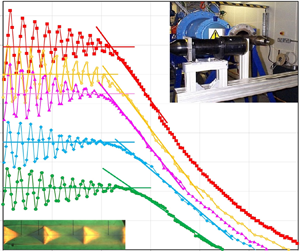
A first indication of the impact of jet heating is provided in figure 16; this presents centreline profiles for all cases considered in the experimental programme (NPR = 2.32). Figure 16 shows development of total temperature (a) and axial velocity (b), with data presented in dimensional format (K, m s−1) to illustrate the magnitude of temperature and velocity considered in these measurements.

Figure 16. Centreline mean total temperature (a) and mean axial velocity, (b) dimensional format, NPR = 2.32 for various NTRs.
For both temperature and velocity, a straight line has been added after the potential core (a best fit least squares approximation to the decay data in the initial ~5D after the velocity/temperature deviate from their values inside the potential core). This indicates the rate of decay in the jet merging region and allows a visual assessment of how jet temperature affects this. This aspect is quantified below, but it is noticeable the rate of decay increases significantly with NTR up to a value of 2.03 but changes much more slowly after that. The velocity oscillations occurring just after nozzle exit indicate small changes in the number of shock cells with NTR; at NTR = 1.0 there were 12 shock diamonds, decreasing to 10 at the higher NTR values. This may be interpreted as a consequence of increased shear layer thickness at higher NTR due to the faster spreading t 1/2-effect. A thicker shear layer leads to increased energy loss when pressure waves reflect at the jet/ambient boundary. The weakened expansion/compression waves that constitute the shock cells causes the amplitude of velocity oscillations to decrease more rapidly, leading to fewer shock cells. The oscillation amplitude of the first shock cell varied only slightly with NTR (16 %–21 % of the core velocity). Figure 16 also shows how Lp reduces as NTR increases, but, as for the jet merging decay rate, little change occurs after NTR = 2.03.
The physical mechanism underpinning the change in temperature and velocity decay slopes seen in figure 16 may be clarified by analysing these as a function of the static temperature ratio of the individual hot jet cases. Figure 17 plots gradient magnitude against the relevant value of t 1/2. This makes it clear that – for both variables – decay rate evaluated form the absolute variable plots increases linearly with t 1/2. This is direct evidence that it is the ((2.2)) static temperature ratio effect which influences spreading rate in the merging jet region.

Figure 17. Centreline total temperature (a) and axial velocity (b) decay rates for NPR = 2.32 at various NTRs.
The observation that raising jet NTR has an initial distinct effect on decay rate, which diminishes rapidly above NTR = 2.03 is shown better by presenting centreline development in non-dimensional form. The normalising reference conditions used are constant in the jet core (Ucore, Tt,core see figure 16), with temperature presented via its increase above ambient conditions:  ${T_{amb}}\textrm{:}\,\Delta {T^\ast } = ({T_{t,cl}} - {T_{amb}})/({T_{t,core}} - {T_{amb}})$.
Considering axial velocity, figure 18(a) uses jet nozzle diameter D as a reference length scale for axial distance, and clearly illustrates an increasing centreline decay rate downstream of Lp up to NTR = 2.03, beyond which the slope remains unchanged. If the varying decay slopes are plotted against their t 1/2 values, a linear relationship is again found, so the dominant flow physics described above is still applicable. However, the reason why the decay rate ceases to increase beyond NTR 2.03 is not apparent. The effect was first observed by Lau (Reference Lau1981), who noted: ‘heating causes axial distributions to move upstream, but this stops above a temperature ratio (t) ~1.5’. In the present data NPR = 2.32 (fully expanded Mj = 1.17) and NTR=2.03 imply t = 1.6, agreeing closely with Lau's observation. In Lau (Reference Lau1981) it was postulated that the cause was ‘shear layer rotation towards the jet axis when heat is applied’, but no physical reasoning was proposed to substantiate this and an alternative explanation is sought below. If x is non-dimensionalised using Lp not only do potential core end points coincide, but this also effectively collapses downstream decay onto a single curve (figure 18b). This implies that the strength of t influence on both Lp and velocity decay is similar.

Figure 18. Centreline mean axial velocity, vs x/D (a), vs x/Lp (b). (c) Centreline mean total temperature.
In stark contrast to this, non-dimensional total temperature decay already collapses onto a single line when plotted against x/D (figure 18(c) – some variation can be seen downstream, but this is small. Changing x/D to x/Lp for temperature would have the opposite effect as for velocity, moving the curves apart. Thus, temperature ratio clearly has a different effect on velocity and scalar properties. Turbulent mixing in free shear flows for scalar properties is known to be different to momentum mixing – in Reynolds averaged Navier–Stokes (RANS) eddy viscosity models for jet flows, for example, values of the turbulent Prandtl number are typically 0.5–0.7. However, the precise cause of this behaviour in hot high Mj jets is unclear from the current measurements. Additional data on turbulent heat fluxes as well as Reynolds shear stress are needed to clarify this or LES investigations of hot high-speed jets might provide an explanation.
The diminishing effect of temperature ratio is also visible in the turbulence field. Figure 19(a) presents centreline development of non-dimensional axial turbulence r.m.s. for all five NTR cases. Bridges & Wernet (Reference Bridges and Wernet2010) had previously commented that addition of heat increases peak turbulence level (although only by ~5 %) and moves this forward as Lp decreases with jet heating. Figure 19(a) confirms these observations, but again the response to increasing NTR ceases beyond NTR = 2.03. To demonstrate that the turbulence has not reached its self-similar state in the jet near field, figure 19(b) shows axial r.m.s. data non-dimensionalised using the local centreline axial mean velocity. Self-similarity would imply that this asymptotes to a constant value in the jet far field (~28 % on the centreline for a constant density turbulent jet (Hussein, Capp & George Reference Hussein, Capp and George1994). Figure 19 shows that in the present near-field flow the axial turbulence at all NTRs is approaching this level but has some way to go before entering the far-field region proper.

Figure 19. Centreline axial r.m.s. velocity (non-dimensional), NPR = 2.32 for various NTRs Normalising reference velocity; (a) Ucore, (b) Ucl.
A more plausible explanation for the decreasing response to jet heating is now proposed based on the interplay between t 1/2-based and compressibility-based influences on jet spreading (§§ 2.1 and 2.2). The former increases shear layer spreading rate whereas the latter decreases it. Thus, at particular combinations of NPR and NTR (Mj and t) the first ((2.2)) and second (figure 1) effects may cancel out. More analysis of the data is required to examine this hypothesis, this is presented below in § 4.3 and figure 23 which confirm this speculation as correct.
Finally, figure 20 provides a comparison of measured radial profiles of axial velocity for hot and unheated jets (NTR = 2.03 and NTR = 1.0). Three downstream locations are chosen: close to nozzle exit (x/D = 1.0), close to potential core end (x/D = 6.0), and in the developing jet plume (x/D = 12.0), The data are here normalised using local centreline axial velocity (Ucl) in order to focus attention on profile shape and radial spread. Given the good symmetry displayed in figures 13–15 only positive z data are included. At the first location profiles are very similar; small differences are visible in the jet core, where the hot jet has slightly higher values in excess of 1.0 than the cold jet – and in the thin shear layer – where the hot jet appears slightly narrower. The former occurs because heating changes shock cell length, and a fixed axial station is then shifted relative to the expansion/compression pattern. The latter can be explained if, in this region, the compressibility effect is stronger than the t 2/2-effect. The hot jet has a larger Mc (by ~28 %) and thus has a lower shear layer spreading rate than the cold jet. This scenario persists for the whole of the potential core length, since at x/D = 6.0 the hot jet profile is clearly narrower. The situation is reversed, however, at x/D = 12.0. Since Mc decreases rapidly after the potential core, the balance between compressibility and t 1/2-effects changes and figure 20(a) shows the hot jet profile radially outboard of the cold jet, which corresponds to the faster decay rate of the hot jet in this region.

Figure 20. Non-dimensional profiles, 3 axial stations: (a) axial velocity, (b) shear stress NPR = 2.32 for NTR = 2.03 and 1.00.
Figure 20(b) presents Reynolds shear stress profiles for the same three axial locations. These are fully consistent with the explanation provided above. At x/D = 1.0 the two profiles are effectively the same with the peak value marginally smaller for the hot jet. At x/D = 6.0 peak shear stress is radially inboard location of zero stress suggesting a narrower hot jet, whereas this is beginning to reverse in the stress profiles at x/D = 12.0. These results provide strong evidence for the interplay between compressibility and t 1/2 effects on turbulent mixing, suggesting the former dominates until potential core end, but the latter controls flow development in the jet merging region.
4.3. Analysis of shear layer spread rate $({\delta ^{\prime}_\omega })$ and potential core length (Lp)

Measured radial profiles for NPR = 2.32/NTR = 2.03 at 10 axial stations from nozzle exit to x/D = 16 were post-processed to extract shear layer growth rate using the Brown & Rosko (Reference Brown and Rosko1974) definition: ${\delta _\omega } = {U_{core}}/{(\partial U/\partial z)_{max}}$. An illustration of the accuracy with which measurements resolve the gradient maximum is shown in figure 21(a) for two axial stations. The potential core end is located just downstream of x/D = 6.0 for this flow case, and least-squares best fit straight lines were fitted to identify shear layer growth rate (upstream of Lp) and merging jet growth rate (downstream), figure 21(b). The slope of the line increased by 16 % in the downstream zone, showing a different growth characteristic. Note that this also underlines the risk of error if shear layer growth rate is taken from a single profile at potential core end as in Bridges & Wernet (Reference Bridges and Wernet2010).

Figure 21. (a) Illustration of maximum gradient evaluation at two axial stations. (b) Shear layer and merging jet growth rates.
Compressibility effects on hot jet shear layer spreading rate data have been analysed following the concept proposed in the compressibility-induced reduction diagram of figure 1. To remove the t 1/2 influence on the hot jet spreading rate at any Mc/t combination,  ${\delta ^{\prime}_\omega }({M_c},t)$ must be expressed relative to the incompressible growth rate at the same value of t, i.e. ${\delta ^{\prime}_\omega }(0,t)$. Analysing planar shear layer data in this manner enabled Barone et al. (Reference Barone, Oberkampf and Blottner2006) to identify a correlation which successfully isolated compressibility effects in flows with a wide range of t 0.9–9.0. ${\delta ^{\prime}_\omega }(0,t)$ in the current work from was taken the Brown & Rosko (Reference Brown and Rosko1974) experiments ((2.2)). The present measurement at NTR = 2.03 and the heated jet data of Lau (Reference Lau1981), Seiner et al. (Reference Seiner, Ponton, Jansen and Lagen1992), and Bridges & Wernet (Reference Bridges and Wernet2010) have been added to the unheated data of Lau et al. (Reference Lau, Morris and Fisher1979) and Feng & McGuirk (Reference Feng and McGuirk2016) to produce figure 22 (which also includes the Barone et al. (Reference Barone, Oberkampf and Blottner2006) planar shear layer correlation.)

Figure 22. Compressibility-induced shear layer growth rate reduction for hot jets.
For each data set the aerodynamic operating parameters considered are given, to indicate the wide range of conditions covered: NPR = 1.1–3.1 and NTR = 1.0–3.2, spanning the range of interest for aeronautical propulsion applications. Figure 22 confirms that hot jet shear layer data also lie below the planar shear layer correlation; high-speed jets at any temperature ratio experience an earlier onset of compressibility damping and a larger reduction for given Mc than 2D planar shear layers. The jet data do not extend to higher Mc where the planar curve shows damping to level off. However, since the physical mechanism which underpins damping is the same in planar and annular shear layers, there seems no reason why this should not be repeated, with growth rate reduction asymptoting to a constant value as the convective Mach number exceeds 1.0. although with a lower asymptotic value. A dashed line has been added to extrapolate a possible curve beyond the range of currently available data.
Whilst scatter is clearly present, 70 % of the data (25 out of 36 data points) display a discernible trend, with a few outliers. These outliers consist of the highest temperature ratio (t = 2.3) data of Lau (Reference Lau1981) (black crosses) and the data of Bridges & Wernet (Reference Bridges and Wernet2010) (purple symbols). There seems to be no reason why the normalisation process (using  ${\delta ^{\prime}_\omega }(0,t)$) should fail to eliminate the influence of t for the Lau data (black crosses) when it successfully achieves this for all other Lau data (t = 0.85–1.68). Doubt has already been expressed on the Lau highest t data and entering the data into this diagram seems to confirm this. Most of the Bridges & Wernet (Reference Bridges and Wernet2010) data lie well below the main group of data points. The different method adopted in this study to calculate ${\delta ^{\prime}_\omega }$ probably contributes to this discrepancy. In addition, the effect of t in this data is rather puzzling. The data imply that, for constant Mc, increasing t reduces rather than increases ${\delta ^{\prime}_\omega }$, contrary to expectations. For these reasons, these outlier points have been excluded in generating the ‘best-fit’ correlation of the jet data shown as a solid red line in figure 22. This corresponds to the simple relation (note that this has only been assumed up to Mc = 0.6, beyond this the asymptotic trend at high M will begin to influence the correlation shape)
 \begin{equation}\frac{{{{\delta ^{\prime}}_\omega }({M_c},t)}}{{{{\delta ^{\prime}}_\omega }(0,t)}} = 1 - M_c^2\quad \textrm{(for:}\,\textrm{0} \le {M_c} \le 0.6).\end{equation}
This may be transformed into an equation for  ${\delta ^{\prime}_\omega }$ in terms of Mj and t using (2.2) and (2.5) so it may be directly compared to the Lau (Reference Lau1981) correlation ((2.9))
 \begin{equation}{\delta ^{\prime}_\omega }({M_j},t) = 0.0825(1 + {t^{1/2}})\left[ {1 - \frac{{M_j^2}}{{{{(1 + {t^{{{ - 1} / 2}}})}^2}}}} \right].\end{equation}
 Parameters Mj and t appear in quite different functional forms in (2.9) and (4.2); the correlations are compared for relevant ranges of these variables in figure 23 (note that, for the current study, the curves have been generated using (4.2) for 0.0 < Mc < 0.6 and the dashed extrapolated curve in figure 22 for higher Mc) The two correlations agree quite well for t values 0.8–1.5, but at higher t totally different descriptions of compressibility and t 1/2 influences on  ${\delta ^{\prime}_\omega }$ appear. In Lau (Reference Lau1981), (2.9) was shown to fit the data generated in that study accurately. However, because it was forced to fit the highest t = 2.3 data, which have been shown to display an incorrect compressibility effect in figure 22, implausible aspects result: ${\delta ^{\prime}_\omega }$ increases with t up to t = 1.5 (as expected) but then decreases rapidly with t (curves for t = 0.8 and 2.0 are identical) and produces negative ${\delta ^{\prime}_\omega }$ at low Mach number for t = 3.0. Similarly, the trend with increasing Mj appears correct for lower t values but shows an unphysical increase in ${\delta ^{\prime}_\omega }$ for t = 3.0.

Figure 23. Shear layer growth rate correlations, (a) present and (b) Lau (Reference Lau1981).
In contrast, the current correlation (figure 23a) fully supports the proposal made above of counterbalancing effects of compressibility and t 1/2 effects. At lower Mach numbers strong compressibility damping with increasing Mj is plainly visible for all values of t; the tendency for increasing t to increase growth rate is also visible, although with decreasing effect as Mj increases. For Mj > 1.1 the two effects balance out and the growth rate remains approximately the same for all values of t. This result supports the proposal described above for interplay between Mc-effects and t-effects.
Unfortunately, knowledge of the shear layer spreading rate alone is insufficient to allow accurate estimation of potential core length. Nozzle exit effects may only be influential for a relatively short length, but this may contribute a non-negligible effect on Lp. LES studies by Bogey & Bailly (Reference Bogey and Bailly2010) and measurements by Fontaine et al. (Reference Fontaine, Elliott, Austin and Freund2015) have quantified the Lp variations that various nozzle exit conditions can cause. The former considered laminar boundary layers of various thicknesses; if no disturbances were superimposed large Lp changes (3.3–8.4D) resulted when thickness was increased from 1 %–10 %D. If disturbance was added to simulate turbulence, for a fixed thickness (2.5 %D), Lp changed by up to 0.9D depending on the disturbance strength. The experiments of Fontaine et al. (Reference Fontaine, Elliott, Austin and Freund2015) compared nozzle exit boundary layers with laminar (H = 2.18) and turbulent (H = 1.5) shape factors. An Lp increase from 7.13D to 7.9D was observed (laminar or low Re exit conditions usually produce shorter potential cores). To add to this effect, radial spread in the vicinity of the potential core end will be influenced by the jet merging process, and evidence of turbulent shear stress variations in this region were noted in figure 15(a). Comparison of Lp data taken in various experimental facilities is also problematic due to differences in Lp definition. Evidently, some scatter of measured Lp values is inevitable, since exit boundary layer and Reynolds number effects will vary between facilities unless careful control measures are adopted. It thus seems likely that Lp variations of at least 0.5–1.0D are possible for nominally the same jet condition even without jet heating.
In figure 24 measurements of Lp have been extracted from available experimental studies of high-speed jets at various temperature ratios: Lau (Reference Lau1981), Seiner et al. (Reference Seiner, Ponton, Jansen and Lagen1992), Kearney-Fischer, Kim & Samimya (Reference Kearney-Fischer, Kim and Samimya2009) and the current work; jet Mach number for each data set is indicated. The data are broadly ordered following increasing Mj. All data sets display the feature of upstream movement of Lp with increasing t but a rapid reduction in the strength of this movement after t > ~1.5. This is consistent with the interplay between compressibility and static temperature ratio effects discussed above.

Figure 24. Experimental data for potential core length.
The response of Lp to variations in Mj and t has been assessed by analysing the data in the same manner as the shear layer growth rate. To focus first on compressibility, figure 25 examines Lp data corresponding to isothermal operating conditions, i.e. Lp(Mj, 1) (interpolating between NTR values where necessary). These suggest a strongly nonlinear effect of Mj. It should be noted that some difference between the current and other measurements appears in this figure for supersonic Mj. The present Lp measurement for NPR = 1.0 (i.e. properly expanded) agrees well with all the trend observed in other data at both subsonic and (properly expanded) supersonic conditions. The current measurement at the improperly expanded NPR = 2.32 condition shows a larger value for Lp by ~1D. This is the first indication that, at least for potential core length, the presence of shock cells has had an effect; the agreement at NPR = 1.0 implies the different approach adopted in the current study to management of nozzle exit conditions is unlikely to be the source of the discrepancy at higher NPR.

Figure 25. The Lp(Mj, 1) data and curve fit.
To generate an appropriate curve fit to the data in figure 25 a value for incompressible isothermal flow Lp (0,1) is first added to the data set. The subsonic correlation of Witze (Reference Witze1972) suggested a value of 4.38D and the Lau et al. (Reference Lau, Morris and Fisher1979) correlation 4.2D; averaging these, Lp (0,1) = 4.3 has been used in the curve fit shown in figure 25, leading to the following correlation:
 \begin{equation}\frac{{{L_p}({M_j},1)}}{D} = 4.3 + M_j^{2.5}.\end{equation}
 Following a similar procedure, figure 26 isolates the effect of t by calculating  ${L_p}({M_j},t)/{L_p}({M_j},1)$ for each data set. This shows a reduction of Lp following a ${t^{ - 0.2}}$ relation. The combined correlation which results is
 \begin{equation}\frac{{{L_p}({M_j},t)}}{D} = (4.3 + M_j^{2.5}){t^{ - 0.2}}.\end{equation}
Figure 26. The Lp(Mj, t) data and curve fit.
Equation (4.4) is compared in figure 27 with the correlation proposed by Witze (Reference Witze1972) – (2.6) for subsonic and (2.7) for supersonic conditions. The Lau correlation has not been included since this does not contain any continuous relation with t which is clearly required by the experimental data. Considerable disagreement is apparent in figure 27. The two correlations agree reasonably well for Mj = 0.5 and 0.9, but for supersonic Mj the Witze correlation shows a too slow increase in Lp with Mj and a too steep decrease with t.

Figure 27. The Lp(Mj, t) correlations of Witze (Reference Witze1972) (dashed lines) and current (solid lines).
The success of the current correlation in capturing the response of Lp to changes in Mj and t is indicated by comparison with measurements in figure 28. Trends with both Mach number and temperature ratio are well represented. As for t = 1.0 in figure 25, current data for Mj = 1.17 at various NTR follow the same trend with t as other data but lie 0.5–1.4D above the line provided by the current correlation. This is a further indication of possible effects of improper expansion being influential. Assessment of the hot jet annular shear layer growth shown in figure 22 indicated this was not affected by the presence of shock structures. It is possible, however, that, although shock oscillation strength weakens as the potential core end is approached, the early stage of shear layer development into a merged jet may be modified by the presence of shocks in an improperly expanded jet and thus influence Lp. Some evidence to support this possibility was seen in the shear stress profile at x/D = 4.0 in figure 15(a). More measurements in the region of jet merging are required to identify the precise reason for potential core length sensitivity to improper expansion effects.

Figure 28. The Lp(Mj, t) correlation (lines) compared to measurements (symbols).
5. Concluding remarks
Extensive experimental and analytical research exists for compressibility and temperature ratio effects in two-dimensional turbulent shear layers. To date, however, this has not provided the required understanding of hot, high-speed, jet near-field aerodynamics. A measurement programme was thus undertaken to provide relevant information on the effect of heat addition on high Mach number jets. Analysis of mean velocity, temperature and turbulence data provided clear evidence of the interplay between compressibility and temperature ratio on near-field development. Compressibility-induced shear layer growth rate reduction in hot jets followed a similar trend as observed in previous cold jet data, although displaying an enhanced effect of convective Mach number (MC) compared to planar shear layers. The counter-balancing of compressibility and static temperature ratio (t) effects was shown to explain the observation of a distinct influence of t but with diminishing effect at high MC. Accounting for this counter-balancing feature also enabled an empirical correlation for potential core length (Lp) to be derived that fitted available experimental data for jet Mach numbers Mj = 0.5–2.0 and static temperature ratios t = 0.6–2.5.
The current under-expanded jet data for Lp did not fit the Lp correlation derived. This may be due to the interaction between the embedded shock system and the turbulent mixing which accompanies the transition of an annular shear layer into a merged jet, but more measurements are needed. Other experimental investigations suggested by the current work are: (i) for higher MC values to confirm the extrapolated part of the proposed compressibility–damping correlation, and (ii) for turbulent heat flux to explain the dramatically different response of scalar and momentum properties in the jet merging region to increased jet temperature. The measurements described here represent important validation data for LES CFD models aimed at achieving aerospace propulsion nozzle designs with reduced IR-signature and jet noise properties. In particular, well-resolved simulations of internal nozzle acceleration or other means to prescribe accurate nozzle exit conditions should be explored.
Acknowledgements
The authors are grateful for the technical discussions on the content of his paper with colleagues at Loughborough University: Drs M. Brend and C. Bonham and Professor G. Page.
Funding
This work was funded by EPSRC (Grant No GR/S27467/01).
Decleration of interest
The authors report no conflict of interest.


 Open access