


1 Introduction
Inertia-dominated rough-wall turbulence figures prominently in engineering and geophysical flows; in engineering flows, roughness affects thermal efficiency and aero-/hydro-dynamic performance of lifting surfaces, while roughness in geophysical flows affects, for example, land–atmosphere interactions and benthic sequestration rates in the ocean bottom-boundary layer. For turbulent wall flow of depth,  $\unicode[STIX]{x1D6FF}$, over a spatially homogeneous roughness distribution with characteristic amplitude, $h$, the ratio, $\unicode[STIX]{x1D6FF}/h$, regulates outer (inertial) layer structural attributes; $\unicode[STIX]{x1D6FF}/h\gtrsim 20$ is a well-established lower limit on the presence of outer-layer similarity (Townsend Reference Townsend1976; Jimenez Reference Jimenez2004; Flack, Schultz & Connelly Reference Flack, Schultz and Connelly2007). For $\unicode[STIX]{x1D6FF}/h\lesssim 20$, vortical flow processes emanating from the roughness sublayer attenuate inertial-layer turbulence spatial correlation. Prognostic models for roughness effects are typically based upon a roughness length, $z_{0}=z_{0}(\boldsymbol{X})$, where $\boldsymbol{X}=\{X_{1},X_{2},\ldots ,X_{n}\}$ are geometric attributes of the rough surface; $z_{0}$ can be used within the equilibrium (logarithmic) condition for prediction of Reynolds-averaged streamwise velocity (in this document, the first, second and third components of all vectors are aligned with the streamwise, $x_{1}$, spanwise, $x_{2}$, and wall-normal, $x_{3}$, directions, respectively).
Visualization of heterogeneous roughness cases, where panels (a,e) correspond with canonical spanwise-heterogeneous and IBL cases, respectively, while panels (b–d) are oblique flow–roughness alignment cases. Panel (c) includes annotation of the azimuthal angle origin, based on the Cartesian coordinate system alignment for  $\unicode[STIX]{x1D703}=0$ ( $x_{1}^{\prime }-x_{2}^{\prime }$) and $\unicode[STIX]{x1D703}=\unicode[STIX]{x03C0}/4$ ( $x_{1}-x_{2}$), and showing how panels (a–e) correspond to $\unicode[STIX]{x1D703}=\unicode[STIX]{x03C0}/2$, $3\unicode[STIX]{x03C0}/8$, $\unicode[STIX]{x03C0}/4$, $\unicode[STIX]{x03C0}/8$ and $0$, respectively. Spacing between rows of adjacent high roughness, $s/\unicode[STIX]{x1D6FF}$, noted in panels (a,e). Panel (f) shows a streamwise–wall-normal transect visualization of a prototypical roughness element, which is a vertically truncated, square-based pyramid, and where solid black, dark grey, grey and light grey correspond to cases A1, B1, C1 and D1, respectively (table 1; case discussion to follow).

Spatial heterogeneity in roughness confounds application of traditional roughness metrics. For discussion, we define a roughness heterogeneity composed of ‘stripes’ of relatively high- and low-roughness length,  $z_{0,h}$ and $z_{0,l}$, respectively, where $z_{0,h}$ represents the influence of a distribution of roughness elements with height, $h$, while $z_{0,l}$ represents a surrounding ‘low’ roughness. A range of such cases are shown in figure 1, where panel (a) shows a canonical spanwise-heterogeneous case, for which the flow streamwise direction is aligned parallel to the roughness heterogeneity. Spanwise heterogeneities are responsible for Reynolds-averaged flow heterogeneities (Barros & Christensen Reference Barros and Christensen2014; Vanderwel & Ganapathisubramani Reference Vanderwel and Ganapathisubramani2015; Medjnoun, Vanderwel & Ganapathisubramani Reference Medjnoun, Vanderwel and Ganapathisubramani2018), which are known to be a realization of Prandtl’s secondary flow of the second kind (Anderson et al. Reference Anderson, Barros, Christensen and Awasthi2015a) (discussion to follow). The stripes of elements in figure 1(a–e) could notionally be represented by $z_{0,h}$, while the surrounding white space represents the ‘less rough’ region and could be represented by the lower roughness length, $z_{0,l}$.
Figure 1(e), in contrast, shows a scenario wherein the flow streamwise direction is aligned orthogonal to the heterogeneity. This scenario induces formation of an internal boundary layer (IBL) (Antonia & Luxton Reference Antonia and Luxton1971): an abrupt production of turbulence across the heterogeneity, and associated formation of an internal layer originating at the heterogeneity and thickening in the streamwise direction. In this article, an azimuthal angle,  $\unicode[STIX]{x1D703}$, is introduced to define alignment of the flow streamwise direction relative to the roughness heterogeneity; the origin of the azimuthal angle is selected such that $\unicode[STIX]{x1D703}=\unicode[STIX]{x03C0}/2$ and $0$ correspond to a canonical spanwise heterogeneity (figure 1a) and streamwise heterogeneity (figure 1e), respectively ( $\unicode[STIX]{x1D703}$ and its origin are denoted in figure 1c).
Cases with  $\unicode[STIX]{x1D703}=0$ have received sustained attention for many years, while the flow physics associated with $\unicode[STIX]{x1D703}=\unicode[STIX]{x03C0}/2$ arrangements have, in more recent times, also gained attention. One can envision that scenarios wherein the flow is aligned precisely parallel (figure 1a) or orthogonal (figure 1e) to a roughness heterogeneity are likely the exception, not the norm: cases of practical importance in engineering and geophysics are expected to encounter roughness heterogeneities at oblique angles, i.e. $0<\unicode[STIX]{x1D703}<\unicode[STIX]{x03C0}/2$. Nugroho, Hutchins & Monty (Reference Nugroho, Hutchins and Monty2013) have performed experimental measurement of turbulent boundary layer flow over a ‘herringbone’ roughness pattern, composed of riblets in a converging–diverging pattern; this work is one exception to the sparsity of prior efforts on oblique roughness. However, since Nugroho et al. (Reference Nugroho, Hutchins and Monty2013) consider a distribution wherein lines of convergence and divergence are streamwise aligned and spaced evenly (in the span), this arrangement does not provide a clear basis for assessing flow response to oblique arrangements; indeed, Nugroho et al. (Reference Nugroho, Hutchins and Monty2013) reviewed spanwise–wall-normal distributions of turbulence statistics and flow depth.
In this article, results of large-eddy simulation (LES) of inertia-dominated turbulent channel flow over the arrangements shown in figure 1 are shown. We consider cases with  $\unicode[STIX]{x1D703}=\unicode[STIX]{x03C0}/2$ (figure 1a), $3\unicode[STIX]{x03C0}/8$ (figure 1b), $\unicode[STIX]{x03C0}/4$ (figure 1c), $\unicode[STIX]{x03C0}/8$ (figure 1d) and $0$ (figure 1e); as noted in the following section, use of a pseudospectral LES code necessitates periodicity of the lower boundary, thereby dictating the specific values of $\unicode[STIX]{x1D703}$ considered for this work. In addition to obliquity, $\unicode[STIX]{x1D703}$, the height of roughness elements is also varied; we consider vertically truncated, square-based pyramidal roughness elements (element transect shown in figure 1f). The transition from spanwise-heterogeneous roughness flow response ( $\unicode[STIX]{x1D703}=\unicode[STIX]{x03C0}/2$, figure 1a) to IBL ( $\unicode[STIX]{x1D703}=0$, figure 1e) is nonlinear: IBL-like structure is persistent even for small obliquity values, before vanishing abruptly for pure spanwise-heterogeneous arrangements. A prognostic roughness model is proposed, which incorporates obliquity. An additional roughness parameter affecting aero-/hydro-dynamics of these surfaces is the spacing, $s/\unicode[STIX]{x1D6FF}$, between adjacent rows of relatively high roughness. For simplicity, we consider cases with $s/\unicode[STIX]{x1D6FF}\approx \unicode[STIX]{x03C0}$ for this work (Anderson et al. Reference Anderson, Yang, Shrestha and Awasthi2018) (figure 1a,e shows annotations). Previous work has established that that this spacing is optimal for maintaining $\unicode[STIX]{x1D6FF}$-scale streamwise rolls; herein, our sole focus was reconciling the flow response to variable obliquity for idealized cases.
The LES code and case details are summarized in § 2. Section 3 presents carefully selected LES results, and presents a revised prognostic model designed for variable obliquity. Concluding remarks are presented in § 4. Results of resolution sensitivity testing are provided in Appendix, which demonstrate no discernible influence of computational mesh resolution.
2 Large-eddy simulation: numerical procedure and cases
The spatially filtered incompressible momentum transport equations are solved,  $\text{D}_{t}\tilde{\boldsymbol{u}}(\boldsymbol{x},t)=\boldsymbol{f}(\boldsymbol{x},t)$, where the grid-filtering operation is performed via convolution with the filtering kernel, $\tilde{\boldsymbol{u}}(\boldsymbol{x},t)=G_{\unicode[STIX]{x1D6E5}}\star \boldsymbol{u}(\boldsymbol{x},t)$, where $\widetilde{\ldots }$ denotes a grid-filtered quantity; $\boldsymbol{f}=-\unicode[STIX]{x1D70C}^{-1}\unicode[STIX]{x1D735}p-\unicode[STIX]{x1D735}\boldsymbol{\cdot }\unicode[STIX]{x1D749}+\boldsymbol{e}_{1}\unicode[STIX]{x1D6F1}+\boldsymbol{f}_{b}$, where $\unicode[STIX]{x1D70C}$ is density, $\unicode[STIX]{x1D735}p$ is a pressure correction required to preserve a divergence-free (incompressible) flow, $\unicode[STIX]{x1D735}\boldsymbol{\cdot }\tilde{\boldsymbol{u}}=0$, $\unicode[STIX]{x1D749}=\widetilde{\boldsymbol{u}^{\prime }\otimes \boldsymbol{u}^{\prime }}$ is the subgrid-scale stress tensor, where $\boldsymbol{u}^{\prime }=\boldsymbol{u}-\tilde{\boldsymbol{u}}$, $\unicode[STIX]{x1D6F1}=\unicode[STIX]{x1D70C}^{-1}\text{d}P_{0}/\text{d}x_{1}$ is an imposed pressure gradient and $\boldsymbol{f}_{b}$ is a body force. Note that the shear-normalized viscous stress tensor, $Re_{\unicode[STIX]{x1D70F}}^{-1}\unicode[STIX]{x1D6FB}^{2}\tilde{\boldsymbol{u}}$, is omitted since $Re_{\unicode[STIX]{x1D70F}}=u_{\unicode[STIX]{x1D70F}}\unicode[STIX]{x1D6FF}\unicode[STIX]{x1D708}^{-1}\sim O(10^{7})$ for the inertia-dominated (fully rough) flow conditions typical of geophysical/engineering wall-sheared turbulence, where $u_{\unicode[STIX]{x1D70F}}$ is the shear velocity, $\unicode[STIX]{x1D6FF}$ is flow depth (channel half-height), $\unicode[STIX]{x1D708}$ is kinematic viscosity, and $Re_{\unicode[STIX]{x1D70F}}$ is the roughness Reynolds number. A solenoidal velocity field is maintained by computing the divergence of the momentum transport equation, $\text{D}_{t}[\unicode[STIX]{x1D735}\boldsymbol{\cdot }\tilde{\boldsymbol{u}}(\boldsymbol{x},t)]=\unicode[STIX]{x1D735}\boldsymbol{\cdot }\boldsymbol{f}(\boldsymbol{x},t)$, applying the divergence-free condition, $\unicode[STIX]{x1D735}\boldsymbol{\cdot }\tilde{\boldsymbol{u}}=0$ and solving the resultant pressure Poisson equation with Neumann conditions at the domain top and bottom, $\unicode[STIX]{x2202}\tilde{p}/\unicode[STIX]{x2202}x_{3}|_{x_{3}/\unicode[STIX]{x1D6FF}=1}=0$ and $\unicode[STIX]{x2202}\tilde{p}/\unicode[STIX]{x2202}x_{3}|_{x_{3}/\unicode[STIX]{x1D6FF}=0}=0$, respectively. Spectral discretization is used in the horizontal directions, while vertical gradients are evaluated with centred second-order finite differencing.
The deviatoric component of the subgrid-scale stresses,  $\unicode[STIX]{x1D749}^{d}$, is evaluated using the eddy viscosity modelling approach, $\unicode[STIX]{x1D749}^{d}=\unicode[STIX]{x1D749}-\frac{1}{3}\unicode[STIX]{x1D739}:\unicode[STIX]{x1D749}=-2\unicode[STIX]{x1D708}_{t}\tilde{\unicode[STIX]{x1D64E}}$, where $\unicode[STIX]{x1D708}_{t}=(C_{s}\unicode[STIX]{x1D6E5})^{2}|\tilde{\unicode[STIX]{x1D64E}}|$ is the turbulent viscosity, $C_{s}$ is the Smagorinsky coefficient, $\unicode[STIX]{x1D6E5}$ is the filter size, $\tilde{\unicode[STIX]{x1D64E}}=\frac{1}{2}(\unicode[STIX]{x2202}\tilde{\boldsymbol{u}}+\unicode[STIX]{x2202}\tilde{\boldsymbol{u}}^{\text{T}})$ is the resolved strain-rate tensor and $|\tilde{\unicode[STIX]{x1D64E}}|=(2\tilde{\unicode[STIX]{x1D64E}}\boldsymbol{ : }\tilde{\unicode[STIX]{x1D64E}})^{1/2}$ is the magnitude of the resolved strain-rate tensor. In the present study, $C_{s}$ is evaluated dynamically during LES with the Lagrangian scale-dependent dynamic subgrid-scale (SGS) model of Bou-Zeid, Meneveau & Parlange (Reference Bou-Zeid, Meneveau and Parlange2005). The present LES code has been used in many studies of inertia-dominated, rough-wall turbulence (Anderson et al. Reference Anderson, Barros, Christensen and Awasthi2015a, and references therein); Appendix presents results of resolution sensitivity testing.
The computational mesh is discretized via  $\unicode[STIX]{x1D6E5}_{x_{1}}=L_{x_{1}}/N_{x_{1}}$, $\unicode[STIX]{x1D6E5}_{x_{2}}=L_{x_{2}}/N_{x_{2}}$ and $\unicode[STIX]{x1D6E5}_{x_{3}}=L_{x_{3}}/N_{x_{3}}$, where $\{L_{x_{1}},L_{x_{2}},L_{x_{3}}\}$ is the domain spatial extent and $\{N_{x_{1}},N_{x_{2}},N_{x_{3}}\}$ is the grid resolution. The lower wall momentum fluxes (figure 1) are modelled with a hybrid approach. For locations where $h(x_{1},x_{2})>\unicode[STIX]{x1D6E5}_{x_{3}}/2$ (i.e. an element is protruding into the vertically staggered computational mesh), the drag force imposed on the flow by $h(x_{1},x_{2})$ is captured with the body force, $\boldsymbol{f}_{b}$, appearing in the grid-filtered momentum transport equation (Anderson & Meneveau Reference Anderson and Meneveau2010; Anderson Reference Anderson2012); these regions are conceptually equivalent to ‘more rough’ regions, which would exhibit a relatively larger roughness length (i.e. $z_{0,h}$). For locations where $h(x_{1},x_{2})<\unicode[STIX]{x1D6E5}_{x_{3}}/2$ – i.e. flat regions in figure 1 surrounding the large elements – surface stress is modelled under logarithmic (equilibrium) conditions with baseline roughness length, $z_{0}/\unicode[STIX]{x1D6FF}=5\times 10^{-6}$ (Anderson & Meneveau Reference Anderson and Meneveau2010); in § 1, such regions were defined with the relatively lower roughness length, $z_{0,l}$. This work is, thus, entirely predicated upon local (space–time) efficacy of the logarithmic law (i.e. the presumption of local space–time equilibrium conditions in a complex flow). In the strictest possible sense, local equilibrium never exists, but in recent years there has been widespread use of the logarithmic law in such conditions. Bou-Zeid et al. (Reference Bou-Zeid, Meneveau and Parlange2005) demonstrated that such use of the logarithmic law could be used successfully in channel flows, and many immersed boundary methods leverage the logarithmic law for prescription of peripheral stresses (Graham & Meneveau Reference Graham and Meneveau2012 and references therein). Given the absence of an existing experimental dataset for equivalent cases, the influence of the logarithmic law upon the resultant flow cannot be quantified, nor would such an effort fall within the scope of this work. It is stressed, however, that results from this wall-modelling protocol have been compared against a variety of literature datasets, and in all cases reasonable agreement has been attained (Willingham et al. Reference Willingham, Anderson, Christensen and Barros2013; Anderson, Li & Bou-Zeid Reference Anderson, Li and Bou-Zeid2015b; Zhu et al. Reference Zhu, Iungo, Leonardi and Anderson2016).
The aforementioned LES code has been used to model flow over the cases shown in figure 1, where a transect of the vertically truncated, square-based pyramids is shown in figure 1(f) and the element maximum heights are displayed in table 1. Figure 1(c) shows the obliquity angle and its origin, with the values for specific cases summarized in table 1 (right-most column). Within the main narrative, results will be shown for all cases summarized in table 1, with computational mesh resolution,  $\{N_{x_{1}},N_{x_{2}},N_{x_{3}}\}=\{128,128,128\}$, and spatial extent, $\{L_{x_{1}}/\unicode[STIX]{x1D6FF},L_{x_{2}}/\unicode[STIX]{x1D6FF},L_{x_{3}}/\unicode[STIX]{x1D6FF}\}=\{2\unicode[STIX]{x03C0},2\unicode[STIX]{x03C0},1\}$; for the additional cases reviewed in Appendix, results are shown for LES with equivalent physical attributes to cases A1, A3 and A5, but with $\{N_{x_{1}},N_{x_{2}},N_{x_{3}}\}=\{64,64,64\}$. In all cases, the grid-filtered momentum transport equations are numerically integrated until the flow attains temporal statistical homogeneity; the transport equations are then further advanced to recover Reynolds-averaged turbulence statistics. Turbulence statistics shown herein are based upon a shear-normalized averaging (large-eddy turnover) time, $\unicode[STIX]{x1D6FF}_{t}N_{t}U_{0}\unicode[STIX]{x1D6FF}^{-1}\gtrsim 10^{3}$, where $\unicode[STIX]{x1D6FF}_{t}$ is the dimensional time step, $N_{t}$ is the number of compute time steps associated with time averaging and $U_{0}$ is the dimensional centreline velocity, i.e., $U_{0}=u_{\unicode[STIX]{x1D70F}}\langle \tilde{u} _{1}\rangle _{12t}(x_{3}/\unicode[STIX]{x1D6FF}=1)$. In this article, averaging of any quantity over dimension, $a$, is denoted with $\langle \ldots \rangle _{a}$.

3 Results
Reynolds-averaged streamwise velocity (colour flood, with colour bar for all panels shown at right of panel a) and vertical velocity (line contours, with  $\langle \tilde{u} _{3}\rangle _{t}<-0.07$ and $+0.07$ denoted by blue and red, respectively) transects in the streamwise–wall-normal plane (panels b,d,f,h) and spanwise–wall-normal plane (panels a,c,e,g). Results in panel (a), panels (b,c), panels (d,e), panels (f,g) and panel (h) correspond with case A1, case A2, case A3, case A4 and case A5, respectively. Streamwise–wall-normal and spanwise–wall-normal transects shown at spanwise location, $x_{2}/\unicode[STIX]{x1D6FF}=\unicode[STIX]{x03C0}$, and streamwise location, $x_{1}/\unicode[STIX]{x1D6FF}=\unicode[STIX]{x03C0}$, respectively.
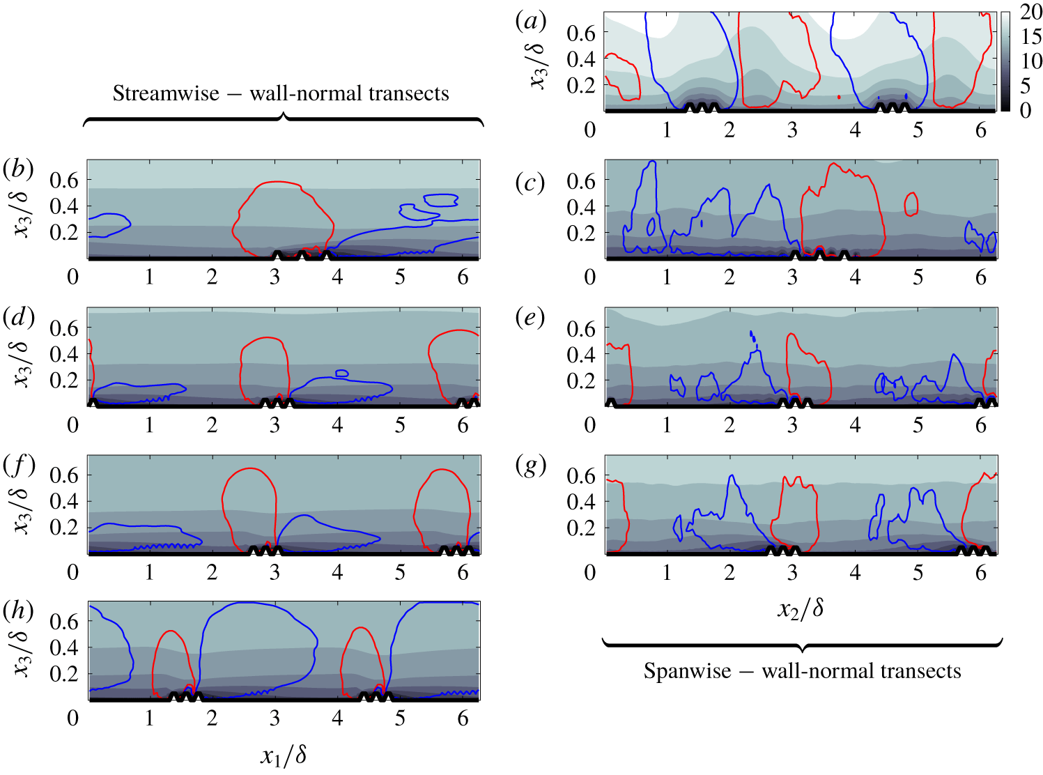
Figure 2 presents Reynolds-averaged distributions of  $\langle \tilde{u} _{1}\rangle _{t}$ and $\langle \tilde{u} _{3}\rangle _{t}$, in the streamwise–wall-normal (b,d,f,h) and spanwise–wall-normal (a,c,e,g) planes. Note that $\langle \tilde{u} _{1}\rangle _{t}$ and $\langle \tilde{u} _{3}\rangle _{t}$ are not shown for case A1 in the streamwise–wall-normal plane, or for case A5 in the spanwise–wall-normal plane. These figures are omitted since they correspond with planes over which the Reynolds-averaged quantities exhibit no heterogeneity, and are thus redundant. Beginning with figure 2(a), which corresponds with a canonical spanwise-heterogeneous roughness, there is a distinct pattern of downwelling and upwelling above relatively more and less rough regions of the surface, which has been widely reported in preceding studies under similar inertial conditions (Willingham et al. Reference Willingham, Anderson, Christensen and Barros2013). Regions of downwelling and upwelling correlate precisely with relative streamwise momentum excess and deficit, respectively, with the former and latter named low- and high-momentum pathways, respectively (Barros & Christensen Reference Barros and Christensen2014). This pattern of downwelling and upwelling is responsible for counter-rotating streamwise rolls, which constitute manifestation of Prandtl’s secondary flow of the second kind (Anderson et al. Reference Anderson, Barros, Christensen and Awasthi2015a). Asymmetry in the low- and high-momentum pathway location (figure 2a) has been reported on numerous previous occasions (Anderson et al. Reference Anderson, Barros, Christensen and Awasthi2015a), and is a natural consequence of the difficulties associated with attaining a true Reynolds average for the slowly varying secondary cells. Note, however, that the pattern of downwelling and upwelling definitively confirms that low- and high-momentum pathways are positioned above the low- and high-roughness regions, respectively. Figure 2(h) shows results for the orthogonal arrangement, case A5, in the streamwise–spanwise plane at $x_{2}/\unicode[STIX]{x1D6FF}=\unicode[STIX]{x03C0}$. The $\langle \tilde{u} _{1}\rangle _{t}$ contours show the ‘standard’ IBL pattern, with plumes of relative momentum deficit thickening in the streamwise, accompanied by downwelling from aloft (Bou-Zeid et al. Reference Bou-Zeid, Meneveau and Parlange2005).
Figure 2(b–g) shows  $\langle \tilde{u} _{1}\rangle _{t}$ and $\langle \tilde{u} _{3}\rangle _{t}$ in the streamwise–wall-normal (b,d,f,h) and spanwise–wall-normal (a,c,e,g) planes, with all transects shown at central out-of-plane locations. Panels (b,c) to panels (f,g) correspond with cases A2 to A4, with A2 being ‘most similar’ to a canonical spanwise heterogeneity and A4 ‘most similar’ to an internal boundary layer. Inspection of $\langle \tilde{u} _{1}\rangle _{t}$ and $\langle \tilde{u} _{3}\rangle _{t}$ in the $x_{1}{-}x_{3}$ plane reveals the persistent nature of IBL-like flow patterns, even for the weakest obliquity (case A2, figure 2b). In this sense, there is no linear transition between IBL and spanwise-heterogeneous flow patterns; this is further appreciated via inspection of $\langle \tilde{u} _{1}\rangle _{t}$ and $\langle \tilde{u} _{3}\rangle _{t}$ in the spanwise–wall-normal plane. Unlike for the spanwise-heterogeneous case (figure 2a), which exhibits distinct downwelling of high-momentum fluid onto the ‘more rough’ regions, downwelling and upwelling fluid is laterally shifted for the oblique arrangements. Moreover, for the canonical spanwise-heterogeneous case, the flow patterns induce counter-rotating streamwise vorticity (evident from the $\langle \tilde{u} _{3}\rangle _{t}$ distribution). For the oblique cases (figure 2b–g), the upwelling–downwelling $\langle \tilde{u} _{3}\rangle _{t}$ distribution is associated with a single roll aligned parallel with the heterogeneity. This pattern of an oblique roll is specific only to these cases with flow–roughness heterogeneity, and will be shown to induce substantial lateral flow.
Reynolds-averaged flow statistics. Panels (a,b) show vertical profiles of plane- and time-averaged streamwise (a) and spanwise (b) velocity for case D1 (lightest grey), D2 (light grey), D3 (grey), D4 (dark grey) and D5 (black), where annotations for obliquity and maximum element height are displayed in panels, for reference. Panel (a) includes a reference logarithmic profile based upon the baseline roughness length,  $z_{0}/\unicode[STIX]{x1D6FF}=5\times 10^{-5}$ (uppermost, thick black line). Panels (c,d) show time-, plane- and depth-averaged streamwise (panel c) and spanwise (panel d) velocity datapoints for all cases, with obliquity on the abscissa, and direction of increasing element height shown (asterisk, square, plus, and circle symbols correspond with cases A1–A5, B1–B2, C1–C5 and D1–D5, respectively).

Figure 3(a,b) shows vertical profiles of plane- and time-averaged streamwise and spanwise velocity, respectively, for cases A1 to A5 (line profiles defined in caption). The location of  $\text{max}(h)/\unicode[STIX]{x1D6FF}$ has been superimposed upon figure 3(a,b), which is helpful for interpreting the inflection in $\langle \tilde{u} _{1}\rangle _{12t}(x_{3})$ and the accumulation in lateral flow evidenced by $\langle \tilde{u} _{2}\rangle _{12t}(x_{3})$. In figure 3(a), the direction of increasing $\unicode[STIX]{x1D703}$ has been added, which confirms a monotonic decrease in momentum penalty, $\unicode[STIX]{x1D6FF}U$, as the flow transitions from IBL to spanwise heterogeneous. Closer inspection shows relatively modest decreases in $\unicode[STIX]{x1D6FF}U$ from the IBL to oblique cases, followed by an abrupt decrease for the spanwise-heterogeneous case (case A1, lightest grey in figure 3a); further discussion to follow. Logarithmic scaling is not evident, nor should it be expected for flow over a rough surface with such extreme spatial heterogeneity. Figure 3(b) shows how lateral flow, $\langle \tilde{u} _{2}\rangle _{12t}(x_{3})>0$, emerges for the oblique cases ( $\langle \tilde{u} _{2}\rangle _{12t}(x_{3})=0$ for cases A1 and A5). The largest lateral flow occurs for $\unicode[STIX]{x1D703}=3\unicode[STIX]{x03C0}/8$ – the largest obliquity angle case (figure 1b) – since this case exhibits weakest IBL-like properties (figure 2), and instead the heterogeneity induces lateral flow.
In order to further appreciate the influence of  $\unicode[STIX]{x1D703}$ and $\text{max}(h)/\unicode[STIX]{x1D6FF}$, figure 3(c,d) shows time- and volume-averaged streamwise velocity, $\langle \tilde{u} _{1}\rangle _{123t}$, and spanwise velocity, $\langle \tilde{u} _{2}\rangle _{123t}$, respectively. Each symbol in figure 3(c,d) represents a table 1 simulation, the abscissa is obliquity and the direction of increasing $\text{max}(h)/\unicode[STIX]{x1D6FF}$ is shown, for reference, in panel (c). In panel (c), it is apparent that increasing element height induces monotonically increasing momentum penalty. When discussing the case A1 to A5 profiles (figure 3a), it was noted that momentum penalty decreases incrementally with increasing obliquity, before an abrupt fall for the case of spanwise heterogeneity; this pattern is persistent with increasing $\text{max}(h)/\unicode[STIX]{x1D6FF}$, evidenced by the sudden rise in $\langle \tilde{u} _{1}\rangle _{123t}$ from $\unicode[STIX]{x1D703}=3\unicode[STIX]{x03C0}/8$ to $\unicode[STIX]{x1D703}=\unicode[STIX]{x03C0}/2$. The pattern of lateral flow with $\unicode[STIX]{x1D703}$ is consistent across cases, with the largest value associated with $\unicode[STIX]{x1D703}=3\unicode[STIX]{x03C0}/8$ (figure 3b,d). Note, too, that the datapoints at $\unicode[STIX]{x1D703}=3\unicode[STIX]{x03C0}/8$ show monotonic increase in lateral flow with increasing $\text{max}(h)/\unicode[STIX]{x1D6FF}$.
The topographically induced development of a Reynolds-averaged spanwise velocity component may lead readers to wonder how this affects the fundamental arguments upon which the LES code (§ 2) is based. During LES, the flow is forced by a non-dimensional pressure gradient,  $\boldsymbol{e}_{x}\unicode[STIX]{x1D6F1}$. For the case of canonical channel flow over a ‘sandpaper’ roughness, $\boldsymbol{e}_{x}\unicode[STIX]{x1D6F1}$ is opposed by a Reynolds-averaged wall stress related directly to $u_{\unicode[STIX]{x1D70F}}$; upon attaining time stationarity, this $u_{\unicode[STIX]{x1D70F}}$ would be used as a normalizing velocity. The presence of a finite $\langle \tilde{u} _{2}\rangle _{t}(\boldsymbol{x})$ indicates a redistribution of
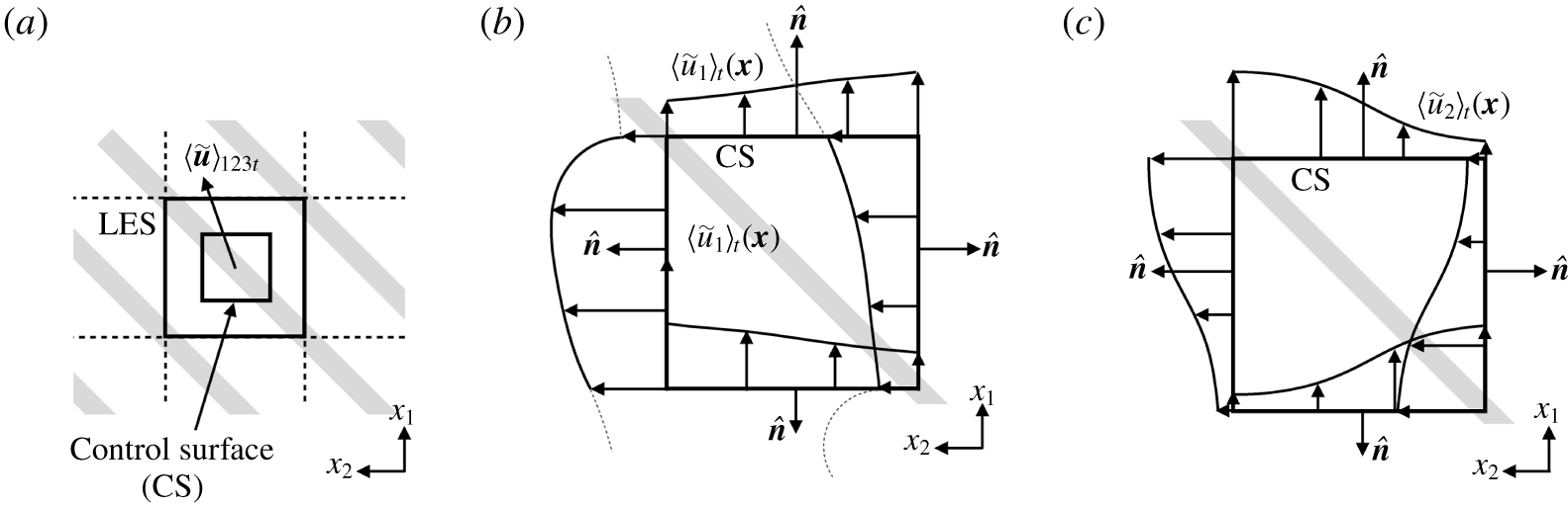
  $\boldsymbol{e}_{x}\unicode[STIX]{x1D6F1}$, which can be readily understood through consideration of a control volume, as shown in figure 4(a). Panel (a) shows the outer LES domain and inner control volume, and topographically induced ‘flow steering’ denoted by time- and volume-averaged velocity, $\langle \tilde{\boldsymbol{u}}\rangle _{123t}$. Panels (b,c) show idealized profiles of $\langle \tilde{u} _{1}\rangle _{t}(\boldsymbol{x})$ and $\langle \tilde{u} _{2}\rangle _{t}(\boldsymbol{x})$, respectively, across the control volume surface. Along the ‘top’ and ‘bottom’ sides of the panel (b) CS, the profiles show relative excesses and deficits in $\langle \tilde{u} _{1}\rangle _{t}(\boldsymbol{x})$ due to streamwise proximity to the elevated roughness stripe; these profiles are compliant with the idealized $\langle \tilde{u} _{1}\rangle _{t}(\boldsymbol{x})$ distribution along the ‘left’ and ‘right’ sides of the CS. Streamwise development in $\langle \tilde{u} _{1}\rangle _{t}(\boldsymbol{x})$ is responsible for sustenance of the spanwise flow; in panel (b), the dashed grey lines show continuation of the profiles external to the control surface, which demonstrate how nonlinear deceleration and acceleration (with respect to $x_{1}$) enable development of $\langle \tilde{u} _{2}\rangle _{t}(\boldsymbol{x})$; these profiles are informed by preceding insights from groups who have studied IBL processes (Bou-Zeid, Meneveau & Parlange Reference Bou-Zeid, Meneveau and Parlange2004). Panel (c) shows idealized profiles of $\langle \tilde{u} _{2}\rangle _{t}(\boldsymbol{x})$, where the largest values develop across the heterogeneity due to the upwelling and downwelling flow patterns reported in figure 2. With this, application of integral form conservation of linear momentum in $x_{1}$ yields
 $$\begin{eqnarray}\displaystyle {\displaystyle \frac{F_{1}}{\unicode[STIX]{x1D70C}}} & = & \displaystyle \int _{\text{d}^{2}\boldsymbol{x}}\left[\int _{\text{d}\boldsymbol{x}}\unicode[STIX]{x1D6F1}\text{d}\boldsymbol{x}\right]n_{1}\text{d}^{2}\boldsymbol{x}-\int _{\text{d}^{2}\boldsymbol{x}}{\displaystyle \frac{\langle \unicode[STIX]{x1D70F}_{13}^{w}\rangle _{t}(x_{1},x_{2})}{\unicode[STIX]{x1D70C}}}n_{3}\text{d}^{2}\boldsymbol{x}\nonumber\\ \displaystyle & = & \displaystyle \int _{\text{d}^{2}\boldsymbol{x}}\langle \tilde{u} _{1}(\boldsymbol{x},t)\left[\tilde{\boldsymbol{u}}(\boldsymbol{x},t)\boldsymbol{ : }\hat{\boldsymbol{n}}\right]\rangle _{t}\text{d}^{2}\boldsymbol{x}\nonumber\\ \displaystyle & {\approx} & \displaystyle \int _{\text{d}^{2}\boldsymbol{x}}\langle \tilde{u} _{1}(\boldsymbol{x},t)\tilde{u} _{2}(\boldsymbol{x},t)\rangle _{t}\text{d}^{2}\boldsymbol{x},\end{eqnarray}$$
 where  $\hat{\boldsymbol{n}}$ is the unit normal vector over vertical faces of the domain (see also figure 4b,c) and $\langle \unicode[STIX]{x1D70F}_{13}^{w}\rangle _{t}(x_{1},x_{2})$ is the spatial distribution of Reynolds-averaged streamwise–wall-normal wall stress. Integral form conservation of linear momentum in $x_{2}$ yields
 $$\begin{eqnarray}{\displaystyle \frac{F_{2}}{\unicode[STIX]{x1D70C}}}=\int _{\text{d}^{2}\boldsymbol{x}}{\displaystyle \frac{\langle \unicode[STIX]{x1D70F}_{23}^{w}\rangle _{t}(x_{1},x_{2})}{\unicode[STIX]{x1D70C}}}n_{3}\,\text{d}^{2}\boldsymbol{x}=\int _{\text{d}^{2}\boldsymbol{x}}\langle \tilde{u} _{2}(\boldsymbol{x},t)\tilde{u} _{1}(\boldsymbol{x},t)\rangle _{t}\,\text{d}^{2}\boldsymbol{x},\end{eqnarray}$$
 where  $\langle \unicode[STIX]{x1D70F}_{23}^{w}\rangle _{t}(x_{1},x_{2})$ is the spatial distribution of Reynolds-averaged spanwise–wall-normal wall stress. Equations (3.1) and (3.2) confirm that the redistribution of momentum to the spanwise does not lead to an intrinsic violation of momentum conservation; rather, that
 $$\begin{eqnarray}\displaystyle u_{\unicode[STIX]{x1D70F}} & = & \displaystyle \left\{{\displaystyle \frac{1}{L_{x_{1}}L_{x_{2}}}}\int _{\text{d}^{2}\boldsymbol{x}}\left[\int _{\text{d}\boldsymbol{x}}\unicode[STIX]{x1D6F1}\text{d}\boldsymbol{x}\right]n_{1}\text{d}^{2}\boldsymbol{x}\right\}^{1/2}\nonumber\\ \displaystyle & = & \displaystyle \left\{{\displaystyle \frac{1}{L_{x_{1}}L_{x_{2}}}}\displaystyle \int _{\text{d}^{2}\boldsymbol{x}}\left[{\displaystyle \frac{\langle \unicode[STIX]{x1D70F}_{13}^{w}\rangle _{t}(x_{1},x_{2})}{\unicode[STIX]{x1D70C}}}+{\displaystyle \frac{\langle \unicode[STIX]{x1D70F}_{23}^{w}\rangle _{t}(x_{1},x_{2})}{\unicode[STIX]{x1D70C}}}\right]n_{3}\text{d}^{2}\boldsymbol{x}\right\}^{1/2}.\end{eqnarray}$$
 It is, thus, clear that overall forcing (in our case, the non-dimensional pressure gradient), is distributed over the two Reynolds-averaged wall stress terms, but that conservation of linear momentum is nevertheless preserved. Therefore, the flow can be normalized by  $u_{\unicode[STIX]{x1D70F}}$ with no loss of generality. The profiles sketched in figure 4(b,c) show idealized Reynolds-averaged streamwise and spanwise velocity, respectively, which demonstrates how an imbalance between the spanwise flux (panel c) of streamwise momentum (panel b) develops the right-hand side term in (3.1).
Schematic of flow–roughness alignment at oblique angle,  $\unicode[STIX]{x1D703}=\unicode[STIX]{x03C0}/2$, where elevated roughness is denoted by a grey strip. Panel (a) shows computation LES computational domain and interior control volume with perimeter control surface (CS). Panel (a) shows idealized time- and volume-averaged velocity, indicating resultant ‘flow steering’ due to flow–roughness obliquity. Panels (b,c) show idealized profiles of time-averaged streamwise (b) and spanwise (c) velocity, where momentum imbalance highlights the redistribution of streamwise momentum derived for sustenance of the Reynolds-averaged spanwise flow. Panel (b) shows continuation of the streamwise momentum profiles external to the control surface.
To further the preceding results, we now address development of prognostic models for the effective roughness length,  $z_{0,Eff.}$, associated with the present spatially heterogeneous rough surfaces (figure 1, table 1). The intrinsic difficulty posed by this endeavour is a priori correlation of surface geometric details and roughness length; foremost among geometric statistics traditionally used in this effort are height root-mean-square, skewness, plan- and frontal-area index (Jimenez Reference Jimenez2004; Flack et al. Reference Flack, Schultz and Connelly2007)
 $$\begin{eqnarray}\displaystyle \left.\begin{array}{@{}c@{}}\displaystyle \unicode[STIX]{x1D70E}_{h^{\prime }}=(\langle h^{2}\rangle _{12}-\langle h\rangle _{12}^{2})^{1/2},\quad s_{h^{\prime }}={\displaystyle \frac{\langle h^{3}\rangle _{12}-\langle h\rangle _{12}^{3}}{(\langle h^{2}\rangle _{12}-\langle h\rangle _{12}^{2})^{3/2}}},\quad \unicode[STIX]{x1D706}_{p}={\displaystyle \frac{A_{p}}{A_{d}}},\quad \text{and}\\ \displaystyle \unicode[STIX]{x1D706}_{f}={\displaystyle \frac{\displaystyle \mathop{\sum }_{i}^{N_{i}}\mathop{\sum }_{j}^{N_{j}}{\mathcal{R}}(\unicode[STIX]{x2202}_{1}h(x_{i},x_{j}))}{A_{d}}},\end{array}\right\} & & \displaystyle\end{eqnarray}$$
 where  $A_{p}$ is the plan are covered by obstacles, ${\mathcal{R}}(x)=x$ and $0$ if $x\geqslant 0$ or ${<}0$, respectively (ramp function), thereby isolating the cumulative frontal area (i.e. the area ‘seen’ by incoming flow within the roughness sublayer) (Anderson & Meneveau Reference Anderson and Meneveau2010, Reference Anderson and Meneveau2011), and $A_{d}$ is the surface area. Napoli, Armenio & Marchis (Reference Napoli, Armenio and Marchis2008) have demonstrated that an ‘effective slope’ parameter, $ES$, is a promising avenue to prediction of momentum penalty, although for the inertia-dominated (fully rough) cases herein momentum penalty dependence upon $ES$ by definition vanishes. Note that, as defined, $ES=2\unicode[STIX]{x1D706}_{f}$ for the cases considered herein (i.e. the topography is not superimposed upon a non-periodic, large-scale undulation). It may be of interest to generalize the notion of $\unicode[STIX]{x1D706}_{f}$ and $ES$ for the influence of obliquity by defining a streamwise and spanwise component and considering the ratio of the former to the latter
 $$\begin{eqnarray}\unicode[STIX]{x1D706}_{f,1}={\displaystyle \frac{\displaystyle \mathop{\sum }_{i}^{N_{i}}\mathop{\sum }_{j}^{N_{j}}{\mathcal{R}}(\unicode[STIX]{x2202}_{1}h(x_{i},x_{j}))}{A_{d}}}={\displaystyle \frac{1}{2}}ES_{1},\quad \text{and}\quad \unicode[STIX]{x1D706}_{f,2}={\displaystyle \frac{\displaystyle \mathop{\sum }_{i}^{N_{i}}\mathop{\sum }_{j}^{N_{j}}{\mathcal{R}}(\unicode[STIX]{x2202}_{2}h(x_{i},x_{j}))}{A_{d}}}={\displaystyle \frac{1}{2}}ES_{2},\end{eqnarray}$$
and
 $$\begin{eqnarray}\unicode[STIX]{x1D712}={\displaystyle \frac{\unicode[STIX]{x1D706}_{f,1}}{\unicode[STIX]{x1D706}_{f,2}}}.\end{eqnarray}$$
 However, recall that for the present cases, the elements are cubes, and, as such,  $\unicode[STIX]{x1D712}$ is unity for all cases. A future study could address cases with $\unicode[STIX]{x1D712}\neq 1$, which could be attained with topographies composed of rectangular prisms or ellipsoidal elements. Such an effort is beyond the scope of this article, and cannot be addressed herein. For the roughness cases considered in this article (table 1), figure 5(a–c) shows $\unicode[STIX]{x1D70E}_{h^{\prime }}$, $\unicode[STIX]{x1D706}_{p}$ and $\unicode[STIX]{x1D706}_{f}$, respectively. In the ‘engineering’ roughness literature, correlations predicated upon linear scaling with $\unicode[STIX]{x1D70E}_{h^{\prime }}$ are common (Flack & Schultz Reference Flack and Schultz2010):
 $$\begin{eqnarray}z_{0,Eff.}^{1}=f(\unicode[STIX]{x1D70E}_{h^{\prime }(\boldsymbol{x})})=\unicode[STIX]{x1D6FC}\unicode[STIX]{x1D70E}_{h^{\prime }(\boldsymbol{x})},\end{eqnarray}$$
Surface and effective roughness attributes. Panels (a,b,c) show root-mean-square, plan- and frontal-area index, respectively. Panel (d) shows datapoints for effective roughness with (3.7) (solid grey) and (3.8) profiles (solid black); panel (d) inset shows front-area index against maximum height for the case of  $\unicode[STIX]{x1D703}=0$. Symbol usage equivalent to figure 3. Panel (e) shows comparison of (3.8) prediction (abscissa) against existing datasets (ordinate): complex roughness with prominent spanwise heterogeneity (Mejia-Alvarez & Christensen Reference Mejia-Alvarez and Christensen2010; Barros & Christensen Reference Barros and Christensen2014) (square), arrays of multiscale cubic topography (Zhu et al. Reference Zhu, Iungo, Leonardi and Anderson2016) (‘plus’ symbols) and cases considered in this article (‘asterisk’ symbols). Direction of increasing $\text{max}(h)/\unicode[STIX]{x1D6FF}$ noted in panels (a,d).
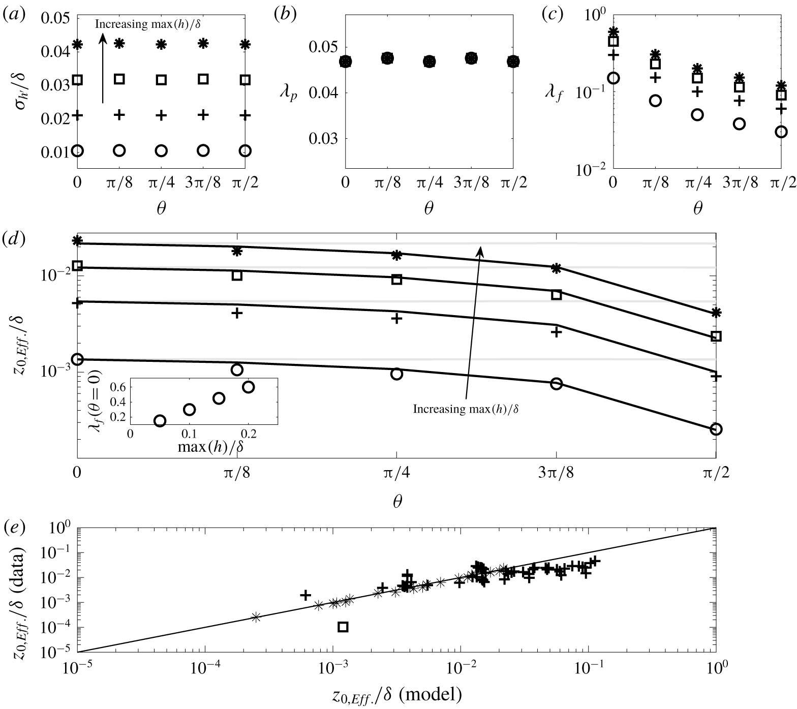
where  $\unicode[STIX]{x1D6FC}\sim O(10^{-1})$ has been consistently reported for an exceptionally broad range of roughness types. It is clear, upon inspection, that $\unicode[STIX]{x1D70E}_{h^{\prime }}$ and $\unicode[STIX]{x1D706}_{p}$ do not capture variable $\unicode[STIX]{x1D703}$, although the preceding results report distinct flow response; the $\unicode[STIX]{x1D70E}_{h^{\prime }}$ datapoints vary with $\text{max}(h)/\unicode[STIX]{x1D6FF}$, but this alone is inadequate for any prognostic model specific to heterogeneous roughness at variable obliquity. Figure 5(c) shows a clear dependence of $\unicode[STIX]{x1D706}_{f}$ upon $\unicode[STIX]{x1D703}$, with the smallest and largest values reported for $\unicode[STIX]{x1D703}=\unicode[STIX]{x03C0}/2$ and $0$, respectively. The previous results have established a dependence upon $\text{max}(h)/\unicode[STIX]{x1D6FF}$ and $\unicode[STIX]{x1D703}$, and to this extent a generalized model based upon the product of independent functions is proposed
 $$\begin{eqnarray}z_{0,Eff.}^{2}=f(\unicode[STIX]{x1D70E}_{h^{\prime }(\boldsymbol{x})},\unicode[STIX]{x1D706}_{f},\unicode[STIX]{x1D703})\approx \unicode[STIX]{x1D6FC}_{1}\unicode[STIX]{x1D70E}_{h^{\prime }(\boldsymbol{x})}p(\unicode[STIX]{x1D706}_{f})q(\unicode[STIX]{x1D703})\approx \unicode[STIX]{x1D6FC}_{1}\unicode[STIX]{x1D70E}_{h^{\prime }(\boldsymbol{x})}\unicode[STIX]{x1D706}_{f}\left[1-\unicode[STIX]{x1D6FC}_{2}\exp (\unicode[STIX]{x1D6FC}_{3}\unicode[STIX]{x1D703})\right],\end{eqnarray}$$
 where  $\unicode[STIX]{x1D6FC}_{1}$, $\unicode[STIX]{x1D6FC}_{2}$ and $\unicode[STIX]{x1D6FC}_{3}$ are empirical constants. The datapoints in figure 5(d) are a posteriori recovered effective roughness lengths, based upon best fit logarithmic profiles to the $\langle \tilde{u} _{1}\rangle _{12t}(x_{3})$ profiles from LES of flow over the table 1 cases. As noted in the discussion accompanying figure 3(a), for some flow–roughness obliquity arrangements $\langle \tilde{u} _{1}\rangle _{12t}(x_{3})$ does not scale with the logarithm of $x_{3}$. However, the reported deviation from logarithmic scaling is not so severe that logarithmic fits cannot be used for the purpose of $z_{0,Eff.}$ recovery. The abscissa is obliquity angle, which demonstrates how these oblique surfaces become ‘less rough’ with increasing $\unicode[STIX]{x1D703}$; similarly, the datapoints show how the surfaces become ‘more rough’ with increasing roughness height amplitude. The figure includes an inset, to illustrate that $\unicode[STIX]{x1D706}_{f}\sim \text{max}(h)/\unicode[STIX]{x1D6FF}$.
As expected,  $z_{0,Eff.}$ decreases abruptly from $\unicode[STIX]{x1D703}=3\unicode[STIX]{x03C0}/8$ to $\unicode[STIX]{x03C0}/2$, which corresponds to the aforementioned regime transition from ‘IBL like’, with an oblique vortex across the heterogeneity, to canonically spanwise heterogeneous (figure 1a, and accompanying text).
The solid grey profiles in figure 5 show predictions of (3.7) with  $\unicode[STIX]{x1D6FC}=0.12$. For the IBL arrangement, this model performs well, but for increasing obliquity a significant divergence emerges, indicating that scaling upon $\unicode[STIX]{x1D70E}_{h^{\prime }}$ alone is inadequate for the current roughness cases. Also included in figure 5 are black profiles, showing predictions from (3.8) with $\unicode[STIX]{x1D6FC}_{1}=0.95$, $\unicode[STIX]{x1D6FC}_{2}=0.1$ and $\unicode[STIX]{x1D6FC}_{3}=1.35$. Equation (3.8) is generalized to incorporate the dependence upon obliquity and roughness amplitude, and we see strong support for this model.
Figure 5(e) shows results of model efficacy testing, where the model and literature data are shown on the abscissa and ordinate, respectively (divergence from the one-to-one line constitutes weaker performance of the model); case details are noted in the caption. The datapoint from Christensen and company (Mejia-Alvarez & Christensen Reference Mejia-Alvarez and Christensen2010; Barros & Christensen Reference Barros and Christensen2014) corresponds to their complex roughness case (Bons et al. Reference Bons, Taylor, McClain and Rivir2001), which features a prominent spanwise heterogeneity. For those experiments,  $u_{\unicode[STIX]{x1D70F}}=0.736~\text{m}~\text{s}^{-1}$ (Mejia-Alvarez & Christensen Reference Mejia-Alvarez and Christensen2010, their figure 4b), $U_{0}=16.9~\text{m}~\text{s}^{-1}$ (Mejia-Alvarez & Christensen Reference Mejia-Alvarez and Christensen2010, their table 2) and boundary layer depth, $\unicode[STIX]{x1D6FF}=100~\text{mm}$ (Mejia-Alvarez & Christensen Reference Mejia-Alvarez and Christensen2010). The author used the Bons et al. (Reference Bons, Taylor, McClain and Rivir2001) topography to compute frontal-area index, $\unicode[STIX]{x1D706}_{f}\approx 0.23$. These numerical values were used to recover $z_{0,Eff.}$a posteriori, which was compared against an (3.8) prediction with $\unicode[STIX]{x1D703}=\unicode[STIX]{x03C0}/2$. There is some disagreement in the predictions, although it is stressed that the Bons et al. (Reference Bons, Taylor, McClain and Rivir2001) topography represents a case of complex, multiscale roughness with a predominant spanwise heterogeneity, which would thus challenge the predictive potential of any model. Unfortunately, comparison against the datasets from Ganapathisubramni and company (Vanderwel & Ganapathisubramani Reference Vanderwel and Ganapathisubramani2015; Medjnoun et al. Reference Medjnoun, Vanderwel and Ganapathisubramani2018) was not possible, since they consider continuous streamwise-aligned rows of LEGO elements, for which $\unicode[STIX]{x1D706}_{f}=\infty$. To further diversify the study, results from a complementary LES investigation have been included in figure 5(e) (Zhu et al. Reference Zhu, Iungo, Leonardi and Anderson2016). These results correspond to flow over distributions of cubic roughness elements under inertia-dominated conditions. Although those cases exhibited no streamwise or spanwise correlation, they nevertheless broaden the scope of comparison, and as seen the agreement is favourable; equation (3.8) with $\unicode[STIX]{x1D703}=0$ was used for these cases.
4 Conclusion
Prior research on roughness has addressed a wide range of topics, from limitations on the presence of outer-layer similarity to roughness sublayer structural properties, and to roughness element geometry influences. IBL dynamics has also been the topic of substantial prior work: IBLs are a product of streamwise roughness heterogeneity, from low-to-high or high-to-low roughness, originate at the surface heterogeneity, and thicken in the downstream before homogenizing via ambient, background shear. Flow response to roughness heterogeneities aligned parallel and oblique to the streamwise direction has received relatively less attention. Recent efforts have revealed the large-scale influence of spanwise heterogeneity, which can induce Reynolds-averaged, depth-scale, streamwise vortical rolls. To our knowledge, no prior effort has specifically considered oblique heterogeneity.
LES was used to explore flow response and roughness characteristics due to flow–roughness heterogeneity aligned at parallel, oblique and orthogonal angles. Results indicate that IBL-like dynamics is persistent, even at ‘weak’ obliquity angles, but vanishes abruptly when the heterogeneity is aligned parallel with the streamwise direction. Associated with this is the emergence of a significant Reynolds-averaged lateral flow for oblique cases – this component is, by definition, zero for IBL and spanwise-heterogeneous cases. Reynolds-averaged streamwise velocity is used to recover effective roughness a posteriori, which is posed against common input arguments for roughness models (height root-mean square, plan- and frontal-area index).
We show that height root-mean-square, a widely used surface geometric statistical measure against which roughness can be correlated, fails to capture roughness effects at oblique angles (skewness would, by definition, also not capture the changing aerodynamic signature of the surface with variable obliquity). Frontal-area index, on the other hand, is a promising quantity for prognostic roughness model development. Height root-mean-square and frontal-area index are used to develop a generalized roughness model, which performs well with changing obliquity and differing roughness amplitudes. Given the sparsity of prior work in this area, comprehensive datasets for model efficacy testing do not exist. The model appears to perform well against the cases considered (Mejia-Alvarez & Christensen Reference Mejia-Alvarez and Christensen2010; Zhu et al. Reference Zhu, Iungo, Leonardi and Anderson2016), though further work is needed to fully generalize the model based on a comprehensive survey of the parameter space. Such an effort is beyond the scope of this article, which is intended as a catalyst for future work in the areas of roughness, wall turbulence and obliquity.
Acknowledgements
This work was supported by the U.S. Air Force Office of Scientific Research, grant no. FA9550-14-1-0394 and grant no. FA9550-19-1-0134. LES modelling was completed via allocation of resources from the Texas Advanced Computing Center at the University of Texas. K. T. Christensen, University of Notre Dame, made insightful comments in the preliminary stages of this work. X. Zhu, The Johns Hopkins University, performed postprocessing of the Zhu et al. (Reference Zhu, Iungo, Leonardi and Anderson2016) dataset, which was used in figure 5(e).
Declaration of interests
The authors report no conflict of interest.
Appendix. Resolution sensitivity
Figure 6 presents a brief sampling of flow statistics from LES modelling of flow over cases A1, A3 and A5 at relatively high  $\{N_{x_{1}},N_{x_{2}},N_{x_{3}}\}=\{128,128,128\}$ and relatively low $\{N_{x_{1}},N_{x_{2}},N_{x_{3}}\}=\{64,64,64\}$ resolution, with further details of profile colour coding and symbol usage summarized in the caption. To quantify resolution sensitivity in a normalized sense, the Reynolds-averaged streamwise velocity for the low-resolution case was extrapolated to the high-resolution grid points, which enables recovery of a difference; the velocities are then normalized by the centreline velocity. In all cases, the differences are minimal ( $|\unicode[STIX]{x1D6FF}\langle \tilde{u} \rangle _{12t}(x_{3})|/\langle \tilde{u} \rangle _{12t}(x_{3}/\unicode[STIX]{x1D6FF}=1)<10~\%$), indicating resolution insensitivity and modelling efficacy. As an additional measure, a posteriori recovered effective roughness lengths for the relatively high- and low-resolution cases are shown in figure 6(b). The roughness lengths agree closely across obliquity angles, providing further support for the scientific conclusions provided herein and prognostic quality of the generalized roughness model (3.8).
Results of resolution sensitivity testing from LES modelling of flow over cases A1, A3 and A5. Panel (a) shows vertical profiles of time- and plane-averaged streamwise velocity difference,  $\unicode[STIX]{x1D6FF}\langle \tilde{u} \rangle _{12t}(x_{3})$, between the LES cases with $\{N_{x_{1}},N_{x_{2}},N_{x_{3}}\}=\{128,128,128\}$ and $\{64,64,64\}$ – where the latter was interpolated onto the former’s grid points before subtraction – and normalized by centreline velocity, $\langle \tilde{u} \rangle _{12t}(x_{3}/\unicode[STIX]{x1D6FF}=1)$, for the high-resolution case; colour usage equivalent to figure 3(a). Panel (b) shows a posteriori recovered effective roughness for $\{N_{x_{1}},N_{x_{2}},N_{x_{3}}\}=\{128,128,128\}$ (circle) and $\{64,64,64\}$ (square).
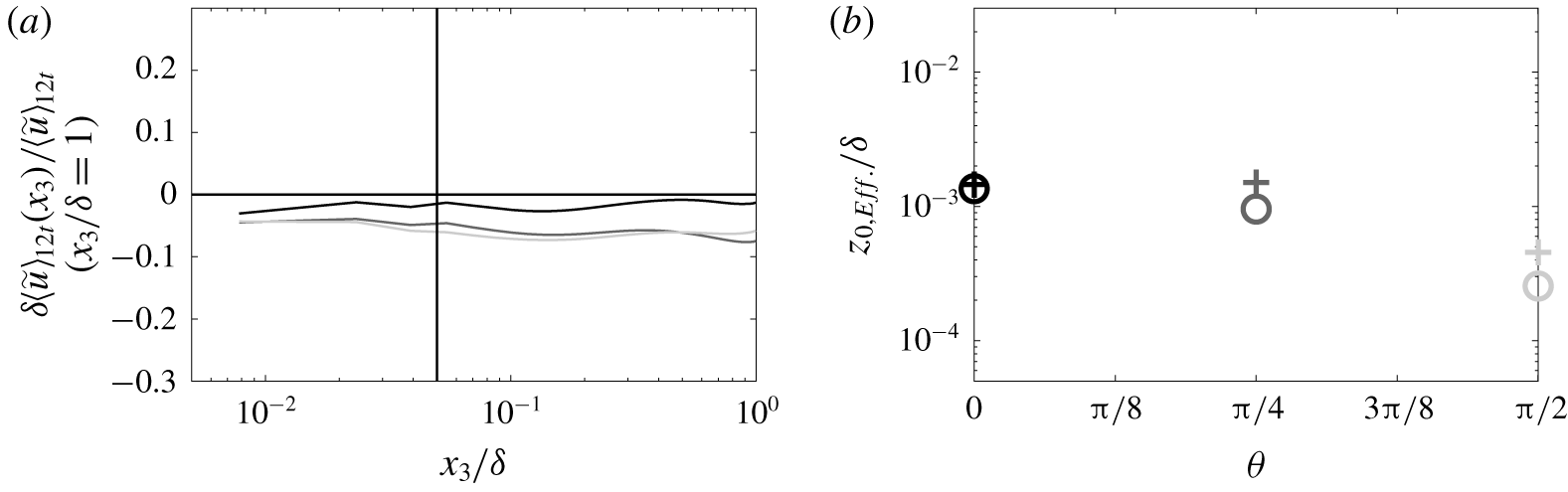


 Open access