 θ
θ Γ
Γ dψ
dψ L2
L2





1. Introduction
Let G be a connected semisimple real algebraic group. Let $\Gamma \lt G$
be a discrete subgroup. Patterson–Sullivan measures are certain families of Borel measures on a generalized flag variety, supported on the limit set of
$\Gamma \lt G$
be a discrete subgroup. Patterson–Sullivan measures are certain families of Borel measures on a generalized flag variety, supported on the limit set of $\Gamma$
. They play a crucial role in the study of dynamics on the associated locally symmetric space, especially in the counting and equidistribution of
$\Gamma$
. They play a crucial role in the study of dynamics on the associated locally symmetric space, especially in the counting and equidistribution of $\Gamma$
-orbits of various geometric objects. The original construction is due to Patterson and Sullivan for Kleinian groups [Reference PattersonPat76, Reference SullivanSul79], which was generalized by Quint [Reference QuintQui02b] (for earlier works, see [Reference AlbuquerqueAlb99] and [Reference BurgerBur93]).
$\Gamma$
-orbits of various geometric objects. The original construction is due to Patterson and Sullivan for Kleinian groups [Reference PattersonPat76, Reference SullivanSul79], which was generalized by Quint [Reference QuintQui02b] (for earlier works, see [Reference AlbuquerqueAlb99] and [Reference BurgerBur93]).
Sullivan showed that for convex cocompact Kleinian groups of $\operatorname{{\rm Isom}}^+(\mathbb H_\mathbb R^n)$
, Patterson–Sullivan measures are Ahlfors regular Hausdorff measures on the limit sets in
$\operatorname{{\rm Isom}}^+(\mathbb H_\mathbb R^n)$
, Patterson–Sullivan measures are Ahlfors regular Hausdorff measures on the limit sets in $\mathbb S^{n-1}$
(see [Reference SullivanSul79, Theorem 8]). Since Patterson–Sullivan measures are constructed from the weighted Dirac measures on an orbit of
$\mathbb S^{n-1}$
(see [Reference SullivanSul79, Theorem 8]). Since Patterson–Sullivan measures are constructed from the weighted Dirac measures on an orbit of $\Gamma$
in the symmetric space
$\Gamma$
in the symmetric space $\mathbb H_\mathbb R^n$
, it is remarkable that they can be given the geometric characterization purely in terms of the internal metric on the limit set of
$\mathbb H_\mathbb R^n$
, it is remarkable that they can be given the geometric characterization purely in terms of the internal metric on the limit set of $\Gamma$
, which is a subset of the boundary
$\Gamma$
, which is a subset of the boundary $\partial \mathbb H_\mathbb R^n\simeq \mathbb S^{n-1}$
.
$\partial \mathbb H_\mathbb R^n\simeq \mathbb S^{n-1}$
.
In recent decades, Anosov subgroups have emerged as a higher-rank generalization of convex cocompact Kleinian groups. Therefore it is natural to ask when the Patterson–Sullivan measures of Anosov subgroups arise as Ahlfors regular Hausdorff measures on the limit sets with respect to appropriate metrics. The main goal of this paper is to answer this question.
To state our results, fix a Cartan decomposition $G=K A^+ K$
, where
$G=K A^+ K$
, where $K \lt G$
is a maximal compact subgroup and
$K \lt G$
is a maximal compact subgroup and $A^+ \subset A$
is a positive Weyl chamber of a maximal real split torus
$A^+ \subset A$
is a positive Weyl chamber of a maximal real split torus $A \lt G$
. We denote by X the associated Riemannian symmetric space
$A \lt G$
. We denote by X the associated Riemannian symmetric space $G/K$
. Let
$G/K$
. Let $\mathfrak g$
and
$\mathfrak g$
and $\mathfrak a$
denote the Lie algebras of G and A, respectively, and set
$\mathfrak a$
denote the Lie algebras of G and A, respectively, and set $\mathfrak a^+=\log A^+$
. Let
$\mathfrak a^+=\log A^+$
. Let $\Pi$
denote the set of all simple roots of
$\Pi$
denote the set of all simple roots of $(\mathfrak g, \mathfrak a)$
with respect to the choice of
$(\mathfrak g, \mathfrak a)$
with respect to the choice of $\mathfrak a^+$
.
$\mathfrak a^+$
.
Fix a non-empty subset $\theta$
of
$\theta$
of $\Pi$
. Let
$\Pi$
. Let $P_\theta$
be the standard parabolic subgroup of G associated with
$P_\theta$
be the standard parabolic subgroup of G associated with $\theta$
. The quotient space
$\theta$
. The quotient space
 $$\mathcal {F}_\theta=G/P_\theta$$
is called the $\theta$
-boundary of X, or a generalized flag variety. We denote by
$\theta$
-boundary of X, or a generalized flag variety. We denote by $\Lambda_\theta$
the limit set of
$\Lambda_\theta$
the limit set of $\Gamma$
in
$\Gamma$
in $\mathcal F_\theta$
(see [Reference BenoistBen97]). For
$\mathcal F_\theta$
(see [Reference BenoistBen97]). For $\theta=\Pi$
, we omit the subscript
$\theta=\Pi$
, we omit the subscript $\theta$
from now on; so, in particular,
$\theta$
from now on; so, in particular, $P=P_\Pi$
is a minimal parabolic subgroup of G. Set
$P=P_\Pi$
is a minimal parabolic subgroup of G. Set $\mathfrak a_\theta=\bigcap_{\alpha\in \Pi-\theta} \operatorname{{\rm ker}}\alpha$
and let
$\mathfrak a_\theta=\bigcap_{\alpha\in \Pi-\theta} \operatorname{{\rm ker}}\alpha$
and let $\mathfrak a_\theta^*$
denote the dual vector space of
$\mathfrak a_\theta^*$
denote the dual vector space of $\mathfrak a_\theta$
. We may think of
$\mathfrak a_\theta$
. We may think of $\mathfrak a_\theta^*$
as a subspace of
$\mathfrak a_\theta^*$
as a subspace of $\mathfrak a^*$
via the canonical projection
$\mathfrak a^*$
via the canonical projection $p_\theta: \mathfrak a\to \mathfrak a_\theta$
(2.3). For
$p_\theta: \mathfrak a\to \mathfrak a_\theta$
(2.3). For $\psi\in \mathfrak a_\theta^*$
, a
$\psi\in \mathfrak a_\theta^*$
, a $(\Gamma, \psi)$
-Patterson–Sullivan measure is a Borel probability measure
$(\Gamma, \psi)$
-Patterson–Sullivan measure is a Borel probability measure $\nu$
on
$\nu$
on $\Lambda_{\theta}$
such that for all
$\Lambda_{\theta}$
such that for all $\gamma \in \Gamma$
and
$\gamma \in \Gamma$
and $\xi \in \Lambda_{\theta}$
,
$\xi \in \Lambda_{\theta}$
,
 $$\frac{d \gamma_* \nu}{d \nu}(\xi) = e^{\psi(\beta_{\xi}(e,\gamma))},$$
where $\beta$
denotes the Busemann map (see (2.8)).
$\beta$
denotes the Busemann map (see (2.8)).
A finitely generated subgroup $\Gamma\lt G$
is called
$\Gamma\lt G$
is called $\theta$
-Anosov if there exists a constant
$\theta$
-Anosov if there exists a constant $C \gt 1$
such that for all
$C \gt 1$
such that for all $\alpha \in \theta$
,
$\alpha \in \theta$
,
 $$\alpha(\mu(\gamma)) \ge C^{-1} |\gamma| - C \quad \text{for all } \gamma \in \Gamma,$$
where $|\cdot |$
is a word metric on
$|\cdot |$
is a word metric on $\Gamma$
with respect to a fixed finite generating set and
$\Gamma$
with respect to a fixed finite generating set and $\mu:G\to \mathfrak a^+$
is the Cartan projection defined by the condition that
$\mu:G\to \mathfrak a^+$
is the Cartan projection defined by the condition that $g \in K ( \exp \mu(g)) K$
for all
$g \in K ( \exp \mu(g)) K$
for all $g\in G$
. For other equivalent definitions of Anosov subgroups, see [Reference LabourieLab06, Reference Guichard and WienhardGW12, Reference Kapovich, Leeb and PortiKLP17, Reference Kapovich, Leeb and PortiKLP18, Reference Guéritaud, Guichard, Kassel and WienhardGGK+17, Reference Bochi, Potrie and SambarinoBPS19], etc.
$g\in G$
. For other equivalent definitions of Anosov subgroups, see [Reference LabourieLab06, Reference Guichard and WienhardGW12, Reference Kapovich, Leeb and PortiKLP17, Reference Kapovich, Leeb and PortiKLP18, Reference Guéritaud, Guichard, Kassel and WienhardGGK+17, Reference Bochi, Potrie and SambarinoBPS19], etc.
In the rest of the introduction, let $\Gamma$
be a non-elementaryFootnote
1
$\Gamma$
be a non-elementaryFootnote
1 $\theta$
-Anosov subgroup of G. We impose the non-elementary assumption on Anosov subgroups for the entire paper. The space of all Patterson–Sullivan measures of
$\theta$
-Anosov subgroup of G. We impose the non-elementary assumption on Anosov subgroups for the entire paper. The space of all Patterson–Sullivan measures of $\Gamma$
is parameterized by the set
$\Gamma$
is parameterized by the set $\mathscr T_\Gamma\subset \mathfrak a_\theta^*$
of all linear forms tangent to the
$\mathscr T_\Gamma\subset \mathfrak a_\theta^*$
of all linear forms tangent to the $\theta$
-growth indicator
$\theta$
-growth indicator $\psi_\Gamma^\theta$
(Definition 3.1):
$\psi_\Gamma^\theta$
(Definition 3.1):
 $$ \mathscr T_\Gamma=\{\psi\in \mathfrak a_\theta^*:\ \psi\ge \psi_\Gamma^\theta, \ \psi(u)=\psi_\Gamma^\theta(u) \ \text{for some } u\in \mathfrak a_\theta-\{0\} \} .$$
More precisely, for any $\psi\in \mathscr T_\Gamma$
, there exists a unique
$\psi\in \mathscr T_\Gamma$
, there exists a unique $(\Gamma, \psi)$
-Patterson–Sullivan measure
$(\Gamma, \psi)$
-Patterson–Sullivan measure
 $$\nu_\psi$$
and every Patterson–Sullivan measure of $\Gamma$
arises in this way (Theorem 3.4). Denote by
$\Gamma$
arises in this way (Theorem 3.4). Denote by $\mathcal L_\theta\subset \mathfrak a_{\theta}^+$
the
$\mathcal L_\theta\subset \mathfrak a_{\theta}^+$
the $\theta$
-limit cone of
$\theta$
-limit cone of $\Gamma$
, which is the asymptotic cone of
$\Gamma$
, which is the asymptotic cone of $p_{\theta}(\mu(\Gamma))$
. Then
$p_{\theta}(\mu(\Gamma))$
. Then $\mathscr T_\Gamma$
is in bijection with the set
$\mathscr T_\Gamma$
is in bijection with the set $\{\psi\in \mathfrak a_\theta^*: \psi\gt 0 \text{on } \mathcal L_\theta-\{0\}\}/\sim$
, where
$\{\psi\in \mathfrak a_\theta^*: \psi\gt 0 \text{on } \mathcal L_\theta-\{0\}\}/\sim$
, where $\psi_1\sim \psi_2$
if and only if
$\psi_1\sim \psi_2$
if and only if $\psi_1=c \cdot \psi_2$
for some
$\psi_1=c \cdot \psi_2$
for some $c\gt 0$
. When the limit cone
$c\gt 0$
. When the limit cone $\mathcal L_\theta$
has non-empty interior (e.g., when
$\mathcal L_\theta$
has non-empty interior (e.g., when $\Gamma$
is Zariski dense in G),
$\Gamma$
is Zariski dense in G), $\mathscr T_\Gamma$
is homeomorphic to
$\mathscr T_\Gamma$
is homeomorphic to $\mathbb R^{\# \theta-1}$
.
$\mathbb R^{\# \theta-1}$
.
1.1 Ahlfors regularity and Hausdorff measures
Anosov subgroups of a rank-one Lie group G are precisely convex cocompact subgroups. In general rank-one groups, the unique Patterson–Sullivan measure of $\Gamma$
is Ahlfors regular and coincides with the Hausdorff measure on
$\Gamma$
is Ahlfors regular and coincides with the Hausdorff measure on $\Lambda$
with respect to a K-invariant sub-Riemannian metric on the boundary
$\Lambda$
with respect to a K-invariant sub-Riemannian metric on the boundary $\partial_\infty X $
which is defined in terms of the Gromov product [Reference CorletteCor90, Theorem 5.4]. Except for the case of
$\partial_\infty X $
which is defined in terms of the Gromov product [Reference CorletteCor90, Theorem 5.4]. Except for the case of $\operatorname{{\rm SO}}(n,1)$
, this sub-Riemannian metric is not a Riemannian metric.
$\operatorname{{\rm SO}}(n,1)$
, this sub-Riemannian metric is not a Riemannian metric.
In this paper, we prove an analogous theorem for a general Anosov subgroup. Let $\psi\in \mathscr T_\Gamma$
. The
$\psi\in \mathscr T_\Gamma$
. The $\theta$
-Anosov property of
$\theta$
-Anosov property of $\Gamma$
implies that any two distinct points of
$\Gamma$
implies that any two distinct points of $\Lambda_\theta$
are in general position and hence the following defines a premetricFootnote
2
on
$\Lambda_\theta$
are in general position and hence the following defines a premetricFootnote
2
on $\Lambda_\theta$
: for
$\Lambda_\theta$
: for $\xi, \eta\in \Lambda_\theta$
,
$\xi, \eta\in \Lambda_\theta$
,
 \begin{equation} d_{\psi}(\xi, \eta) =\begin{cases}e^{-\psi( \mathcal G(\xi, \eta))} & \text{if } \xi \neq \eta,\\ 0 &\text{if } \xi = \eta,\end{cases}\end{equation}
where $\mathcal G$
is the
$\mathcal G$
is the $\mathfrak a$
-valued Gromov product (see Definition 2.3). This premetric turns out to be a correct replacement of the sub-Riemannian metric of the rank-one case.
$\mathfrak a$
-valued Gromov product (see Definition 2.3). This premetric turns out to be a correct replacement of the sub-Riemannian metric of the rank-one case.
For $s \gt 0$
, we denote by
$s \gt 0$
, we denote by $\mathcal H_{\psi}^s$
the s-dimensional Hausdorff measure on
$\mathcal H_{\psi}^s$
the s-dimensional Hausdorff measure on $\Lambda_\theta$
with respect to the premetric
$\Lambda_\theta$
with respect to the premetric $d_\psi$
, which is a Borel outer measure (9.1). We write
$d_\psi$
, which is a Borel outer measure (9.1). We write $\mathcal H_\psi$
for
$\mathcal H_\psi$
for $\mathcal H_\psi^1$
. It turns out that the metric properties of the Patterson–Sullivan measure
$\mathcal H_\psi^1$
. It turns out that the metric properties of the Patterson–Sullivan measure $\nu_\psi$
depend on the symmetricity of
$\nu_\psi$
depend on the symmetricity of $\psi\in \mathfrak a_\theta^*$
:
$\psi\in \mathfrak a_\theta^*$
: $\psi$
is called symmetric if
$\psi$
is called symmetric if $\psi$
is invariant under the opposition involution i of
$\psi$
is invariant under the opposition involution i of $\mathfrak a$
(see (2.2)).
$\mathfrak a$
(see (2.2)).
Our main theorem is as follows.
Theorem 1.1.
Let $\Gamma$
be a non-elementary
$\Gamma$
be a non-elementary $\theta$
-Anosov subgroup of G. Let
$\theta$
-Anosov subgroup of G. Let $\psi\in \mathscr T_\Gamma$
be a symmetric linear form. Then, the Patterson–Sullivan measure
$\psi\in \mathscr T_\Gamma$
be a symmetric linear form. Then, the Patterson–Sullivan measure $\nu_\psi$
is Ahlfors 1-regular and equal to the one-dimensional Hausdorff measure
$\nu_\psi$
is Ahlfors 1-regular and equal to the one-dimensional Hausdorff measure $\mathcal H_\psi$
, up to a constant multiple.
$\mathcal H_\psi$
, up to a constant multiple.
The Ahlfors 1-regularity of $\nu_\psi$
means that there exists
$\nu_\psi$
means that there exists $C\ge 1$
such that for any
$C\ge 1$
such that for any $\xi\in \Lambda_\theta$
and
$\xi\in \Lambda_\theta$
and $0\le r\lt \operatorname{diameter} (\Lambda_{\theta}, d_\psi)$
,
$0\le r\lt \operatorname{diameter} (\Lambda_{\theta}, d_\psi)$
,
 \begin{equation} C^{-1} r\le \nu_\psi (B_{\psi}(\xi, r))\le C r, \end{equation}
where $B_{\psi}(\xi, r)=\{\eta\in \Lambda_{\theta}: d_\psi(\xi, \eta)\lt r\}$
. The premetric space
$B_{\psi}(\xi, r)=\{\eta\in \Lambda_{\theta}: d_\psi(\xi, \eta)\lt r\}$
. The premetric space $(\Lambda_{\theta}, d_{\psi})$
is called Ahlfors s-regular for
$(\Lambda_{\theta}, d_{\psi})$
is called Ahlfors s-regular for $s \gt 0$
if it admits an Ahlfors s-regular Borel measure (see Definition 8.1). Noting that
$s \gt 0$
if it admits an Ahlfors s-regular Borel measure (see Definition 8.1). Noting that $\mathcal H_{s \psi}=\mathcal H_\psi^s$
for
$\mathcal H_{s \psi}=\mathcal H_\psi^s$
for $s\gt 0$
, the reason that the Patterson–Sullivan measure is the one-dimensional Hausdorff measure in the above theorem is due to the normalization of
$s\gt 0$
, the reason that the Patterson–Sullivan measure is the one-dimensional Hausdorff measure in the above theorem is due to the normalization of $\psi$
made by the choice that
$\psi$
made by the choice that $\psi$
is a tangent form, i.e.,
$\psi$
is a tangent form, i.e., $\psi\in \mathscr T_\Gamma$
(see Remark 8.3).
$\psi\in \mathscr T_\Gamma$
(see Remark 8.3).
Remark 1.2. If $\psi$
has gradient in the interior of
$\psi$
has gradient in the interior of $\mathfrak a_{\theta}^+$
, then
$\mathfrak a_{\theta}^+$
, then $\psi$
can be used to define a Finsler metric on X and Dey and Kapovich [Reference Dey and KapovichDK22, Theorem A] have shown that
$\psi$
can be used to define a Finsler metric on X and Dey and Kapovich [Reference Dey and KapovichDK22, Theorem A] have shown that $\nu_\psi$
is the Hausdorff measure, without addressing the Ahlfors regularity (see Remark 9.4). Note that Hausdorff measures need not be Ahlfors-regular in general. Our approach in this paper is different; indeed, we first establish the Ahlfors regularity of
$\nu_\psi$
is the Hausdorff measure, without addressing the Ahlfors regularity (see Remark 9.4). Note that Hausdorff measures need not be Ahlfors-regular in general. Our approach in this paper is different; indeed, we first establish the Ahlfors regularity of $\nu_\psi$
and deduce the rest as a consequence of this.
$\nu_\psi$
and deduce the rest as a consequence of this.
The opposition involution i of $\mathfrak a$
is known to be trivial if and only if G does not have a simple factor of type
$\mathfrak a$
is known to be trivial if and only if G does not have a simple factor of type $A_n$
(
$A_n$
( $n\ge 2$
),
$n\ge 2$
), $D_{2n+1}$
(
$D_{2n+1}$
( $n\ge 2$
) or
$n\ge 2$
) or $E_6$
(see [Reference TitsTit66, 1.5.1]). When i is non-trivial, the symmetricity hypothesis on
$E_6$
(see [Reference TitsTit66, 1.5.1]). When i is non-trivial, the symmetricity hypothesis on $\psi$
cannot be removed. In fact, we prove the following (Theorems 9.2 and 9.12, see also Remark 9.8).
$\psi$
cannot be removed. In fact, we prove the following (Theorems 9.2 and 9.12, see also Remark 9.8).
Theorem 1.3.
Let $\Gamma$
be a Zariski dense
$\Gamma$
be a Zariski dense $\theta$
-Anosov subgroup of G. For any non-symmetric
$\theta$
-Anosov subgroup of G. For any non-symmetric $\psi\in \mathscr T_\Gamma$
, the premetric space
$\psi\in \mathscr T_\Gamma$
, the premetric space $(\Lambda_{\theta}, d_{\psi})$
is Ahlfors s-regular for some
$(\Lambda_{\theta}, d_{\psi})$
is Ahlfors s-regular for some $0\lt s\lt 1$
but the Patterson–Sullivan measure
$0\lt s\lt 1$
but the Patterson–Sullivan measure $\nu_\psi $
is not comparable
Footnote 3
to any
$\nu_\psi $
is not comparable
Footnote 3
to any $\mathcal H_\psi^s$
,
$\mathcal H_\psi^s$
, $s \gt 0$
.
$s \gt 0$
.
1.2 Critical exponents and Hausdorff dimensions
Denote by $\mathcal L_\theta\subset \mathfrak a_{\theta}^+$
the
$\mathcal L_\theta\subset \mathfrak a_{\theta}^+$
the $\theta$
-limit cone of
$\theta$
-limit cone of $\Gamma$
, which is the asymptotic cone of
$\Gamma$
, which is the asymptotic cone of $p_{\theta}(\mu(\Gamma))$
. For
$p_{\theta}(\mu(\Gamma))$
. For $\psi\in \mathfrak a_\theta^*$
which is positive on
$\psi\in \mathfrak a_\theta^*$
which is positive on $\mathcal L_{\theta}-\{0\}$
, we set
$\mathcal L_{\theta}-\{0\}$
, we set
 \begin{equation} \delta_\psi:=\delta_\psi(\Gamma) = \limsup_{T \to \infty} \frac{\log \# \{\gamma \in \Gamma : \psi(\mu(\gamma)) \le T\}}{T}. \end{equation}
The Hausdorff dimension of $(\Lambda_{\theta}, d_{\psi})$
is defined as
$(\Lambda_{\theta}, d_{\psi})$
is defined as
 $$\dim_{\psi} \Lambda_{\theta}:=\inf\{s \gt 0: \mathcal H_{\psi}^{s}(\Lambda_{\theta}) \lt \infty\}. $$
A natural question is whether $\dim_\psi \Lambda_\theta$
is equal to
$\dim_\psi \Lambda_\theta$
is equal to $\delta_\psi$
.
$\delta_\psi$
.
Theorem 1.4.
Let $\Gamma$
be a non-elementary
$\Gamma$
be a non-elementary $\theta$
-Anosov subgroup of G. For any
$\theta$
-Anosov subgroup of G. For any $\psi\in \mathfrak a_\theta^*$
which is positive on
$\psi\in \mathfrak a_\theta^*$
which is positive on $\mathcal L_{\theta}-\{0\}$
, we have
$\mathcal L_{\theta}-\{0\}$
, we have
 $$\dim_{\psi} \Lambda_{\theta}= \delta_{\bar \psi} $$
where $\bar \psi = {\psi + \psi \circ {\rm i}}/{2}$
. In particular, if
$\bar \psi = {\psi + \psi \circ {\rm i}}/{2}$
. In particular, if $\psi$
is symmetric, then
$\psi$
is symmetric, then $\dim_{\psi}\Lambda_{\theta}= \delta_{\psi}$
.
$\dim_{\psi}\Lambda_{\theta}= \delta_{\psi}$
.
Remark 1.5.
-
– We remark that for $\psi$
non-symmetric,
$ \dim_{\psi} \Lambda_{\theta}$
is not equal to
$\delta_\psi $
in general (Proposition 9.10).
$\psi$
non-symmetric,
$ \dim_{\psi} \Lambda_{\theta}$
is not equal to
$\delta_\psi $
in general (Proposition 9.10). -
– As mentioned above, if
$\psi$
is symmetric and the gradient of
$\psi$
belongs to the interior of
$\mathfrak a_{\theta}^+$
, then Theorem 1.4 is due to Dey and Kapovich [Reference Dey and KapovichDK22, Theorem A(v)]. When G is of rank one, Theorem 1.4 is due to Patterson [Reference PattersonPat76], Sullivan [Reference SullivanSul79], and Corlette [Reference CorletteCor90].


Together with a work of Bridgeman, Canary, Labourie, and Sambarino [Reference Bridgeman, Canary, Labourie and SambarinoBCL+15, Proposition 8.1], Theorem 1.4 implies that for any $\psi$
non-negative on
$\psi$
non-negative on $\mathfrak a_\theta^+$
,
$\mathfrak a_\theta^+$
, $\dim_\psi \Lambda_\theta$
depends real-analytically on
$\dim_\psi \Lambda_\theta$
depends real-analytically on $\theta$
-Anosov representations (Corollary 9.13). We describe one concrete example as follows.
$\theta$
-Anosov representations (Corollary 9.13). We describe one concrete example as follows.
1.3 (p,q)-Hausdorff dimension and Teichmüller space
Let $\Sigma$
be a torsion-free uniform lattice of
$\Sigma$
be a torsion-free uniform lattice of $\operatorname{{\rm PSL}}_2(\mathbb R)$
, and let
$\operatorname{{\rm PSL}}_2(\mathbb R)$
, and let $\operatorname{Teich}(\Sigma)$
be the Teichmüller space:
$\operatorname{Teich}(\Sigma)$
be the Teichmüller space:
 $$\operatorname{Teich}(\Sigma)=\{\sigma:\Sigma\to \operatorname{{\rm PSL}}_2(\mathbb R): \begin{matrix} \text{a discrete faithful representation}\end{matrix}\}/ \sim,$$
where the equivalence relation is given by conjugations by elements of $\operatorname{{\rm PGL}}_2(\mathbb R)$
. It is well known that
$\operatorname{{\rm PGL}}_2(\mathbb R)$
. It is well known that $\operatorname{Teich}(\Sigma)\simeq \mathbb R^{6g-6}$
, where g is the genus of the surface
$\operatorname{Teich}(\Sigma)\simeq \mathbb R^{6g-6}$
, where g is the genus of the surface $\Sigma \backslash \mathbb H_\mathbb R^2$
. For
$\Sigma \backslash \mathbb H_\mathbb R^2$
. For $\sigma \in \operatorname{Teich}(\Sigma)$
, denote by
$\sigma \in \operatorname{Teich}(\Sigma)$
, denote by $\Lambda_\sigma\subset \mathbb S^1\times \mathbb S^1$
the limit set of the self-joining subgroup
$\Lambda_\sigma\subset \mathbb S^1\times \mathbb S^1$
the limit set of the self-joining subgroup $(\operatorname{{\rm id}}\times \sigma)(\Sigma)=\{(\gamma,\sigma(\gamma)): \gamma \in \Sigma\}$
, which is well-defined up to conjugations. The Hausdorff dimension of
$(\operatorname{{\rm id}}\times \sigma)(\Sigma)=\{(\gamma,\sigma(\gamma)): \gamma \in \Sigma\}$
, which is well-defined up to conjugations. The Hausdorff dimension of $\Lambda_\sigma$
with respect to a Riemannian metric on
$\Lambda_\sigma$
with respect to a Riemannian metric on $\mathbb S^1\times \mathbb S^1$
is equal to 1 for any
$\mathbb S^1\times \mathbb S^1$
is equal to 1 for any $\sigma\in \operatorname{Teich}(\Sigma)$
(see [Reference Kim, Minsky and OhKMO23, Theorem 1.1]). For any pair (p,q) of positive real numbers, consider the premetric on
$\sigma\in \operatorname{Teich}(\Sigma)$
(see [Reference Kim, Minsky and OhKMO23, Theorem 1.1]). For any pair (p,q) of positive real numbers, consider the premetric on $\mathbb S^1\times \mathbb S^1$
given by
$\mathbb S^1\times \mathbb S^1$
given by
 $$d_{p,q} ( \xi, \eta) = d_{\mathbb S^1}(\xi_1, \eta_1)^p d_{\mathbb S^1}(\xi_2, \eta_2)^q$$
for any $\xi=(\xi_1, \xi_2)$
and
$\xi=(\xi_1, \xi_2)$
and $\eta= (\eta_1, \eta_2)$
in
$\eta= (\eta_1, \eta_2)$
in $\mathbb S^1\times \mathbb S^1$
, where
$\mathbb S^1\times \mathbb S^1$
, where $d_{\mathbb S^1}$
is a Riemannian metric on
$d_{\mathbb S^1}$
is a Riemannian metric on $\mathbb S^1$
. For a subset
$\mathbb S^1$
. For a subset $S \subset \mathbb S^1 \times \mathbb S^1$
, denote by
$S \subset \mathbb S^1 \times \mathbb S^1$
, denote by $\dim_{p,q} S $
the Hausdorff dimension of S with respect to
$\dim_{p,q} S $
the Hausdorff dimension of S with respect to $d_{p, q}$
. Note that on the diagonal of
$d_{p, q}$
. Note that on the diagonal of $\mathbb S^1\times \mathbb S^1$
,
$\mathbb S^1\times \mathbb S^1$
, $d_{p,q}$
is the
$d_{p,q}$
is the $(p+q)$
th power of
$(p+q)$
th power of $d_{\mathbb S^1}$
and hence
$d_{\mathbb S^1}$
and hence
 $$\dim_{p,q} \Lambda_{\operatorname{{\rm id}}}=\frac{1}{p + q}.$$
For each $\sigma \in \operatorname{Teich}(\Sigma)$
, denote by
$\sigma \in \operatorname{Teich}(\Sigma)$
, denote by $\delta_{p, q}(\sigma)$
the critical exponent of the Poincaré series
$\delta_{p, q}(\sigma)$
the critical exponent of the Poincaré series $s\mapsto \sum_{\gamma \in \Sigma} e ^{- s(pd_{\mathbb H_\mathbb R^2}(o, \gamma o) + q d_{\mathbb H_\mathbb R^2}(o, \sigma(\gamma) o))}$
.
$s\mapsto \sum_{\gamma \in \Sigma} e ^{- s(pd_{\mathbb H_\mathbb R^2}(o, \gamma o) + q d_{\mathbb H_\mathbb R^2}(o, \sigma(\gamma) o))}$
.
Corollary 1.6.
Let $p,q \gt 0$
.
$p,q \gt 0$
.
-
(1) For any
$\sigma \in \operatorname{Teich}(\Sigma)$
, we have
$$\dim_{p, q}\Lambda_{\sigma} =\delta_{p,q}(\sigma).$$
-
(2) For any
$\sigma \in \operatorname{Teich}(\Sigma)$
, we have and the equality holds if and only if
$$\dim_{p, q} \Lambda_{\sigma} \le \frac{1}{p + q}$$
$\sigma = \operatorname{{\rm id}}$
.
-
(3) The map
is a real-analytic function on
$$\sigma \mapsto \dim_{p, q}\Lambda_{\sigma} $$
$\operatorname{Teich}(\Sigma)$
.


Part (2) is an immediate consequence of part (1) by the rigidity theorem on $\delta_{p,q}(\sigma)$
, due to Bishop and Steger [Reference Bishop and StegerBS93, Theorem 2] and to Burger [Reference BurgerBur93, Theorem 1(a)]. For a more general version for convex cocompact representations, see Corollary 9.14. If we denote by
$\delta_{p,q}(\sigma)$
, due to Bishop and Steger [Reference Bishop and StegerBS93, Theorem 2] and to Burger [Reference BurgerBur93, Theorem 1(a)]. For a more general version for convex cocompact representations, see Corollary 9.14. If we denote by $f=f_\sigma$
the
$f=f_\sigma$
the $\sigma$
-equivariant homeomorphism
$\sigma$
-equivariant homeomorphism $\mathbb S^1\to \mathbb S^1$
, then
$\mathbb S^1\to \mathbb S^1$
, then $\Lambda_\sigma=\{(x, f(x)):x\in \mathbb S^1\}$
and
$\Lambda_\sigma=\{(x, f(x)):x\in \mathbb S^1\}$
and $\dim_{p,q} \Lambda_\sigma$
can also be understood as the Hausdorff dimension of
$\dim_{p,q} \Lambda_\sigma$
can also be understood as the Hausdorff dimension of $\Lambda_\Sigma=\mathbb S^1$
with respect to the premetric
$\Lambda_\Sigma=\mathbb S^1$
with respect to the premetric $d_{\sigma, p,q} (x,y)= d_{\mathbb S^1}(x,y)^p d_{\mathbb S^1}(f(x), f(y))^q$
,
$d_{\sigma, p,q} (x,y)= d_{\mathbb S^1}(x,y)^p d_{\mathbb S^1}(f(x), f(y))^q$
, $x,y\in \mathbb S^1$
.
$x,y\in \mathbb S^1$
.
1.4 Hausdorff dimension of
$\Lambda_\theta$
with respect to a Riemannian metric

We denote by $\dim \Lambda_\theta$
the Hausdorff dimension of
$\dim \Lambda_\theta$
the Hausdorff dimension of $\Lambda_\theta$
with respect to a Riemannian metric on
$\Lambda_\theta$
with respect to a Riemannian metric on $\mathcal F_\theta$
; since all Riemannian metrics on
$\mathcal F_\theta$
; since all Riemannian metrics on $\mathcal F_\theta$
are Lipschitz equivalent to each other, this is well-defined. With the exception of
$\mathcal F_\theta$
are Lipschitz equivalent to each other, this is well-defined. With the exception of $G=\operatorname{{\rm SO}}^\circ(n,1)$
,
$G=\operatorname{{\rm SO}}^\circ(n,1)$
, $\dim \Lambda$
is not in general equal to the critical exponent of
$\dim \Lambda$
is not in general equal to the critical exponent of $\Gamma$
even in the rank-one case. For a discussion on this for the case of
$\Gamma$
even in the rank-one case. For a discussion on this for the case of $G=\operatorname{SU}(n,1)$
, see [Reference DuflouxDuf17].
$G=\operatorname{SU}(n,1)$
, see [Reference DuflouxDuf17].
From Theorem 1.4, we derive an estimate on $\dim \Lambda_\theta$
in terms of critical exponents. Let
$\dim \Lambda_\theta$
in terms of critical exponents. Let $\chi_{\alpha}$
denote the Tits weight of G associated to
$\chi_{\alpha}$
denote the Tits weight of G associated to $\alpha\in \Pi$
as given in (10.2). When G is split over
$\alpha\in \Pi$
as given in (10.2). When G is split over $\mathbb R$
,
$\mathbb R$
, $\chi_\alpha$
is simply the fundamental weight associated to
$\chi_\alpha$
is simply the fundamental weight associated to $\alpha$
. We prove the following.
$\alpha$
. We prove the following.
Theorem 1.7.
For any $\theta$
-Anosov subgroup
$\theta$
-Anosov subgroup $\Gamma$
of G, we have
$\Gamma$
of G, we have
 $$ \max_{\alpha \in \theta} \delta_{\chi_{\alpha} + \chi_{{\rm i}(\alpha)}} \le \dim \Lambda_{\theta} \le \max_{\alpha \in \theta} \delta_{\alpha} .$$
Moreover, both the upper and lower bounds are attained by some Anosov subgroups.
For $G=\operatorname{{\rm PSL}}_n(\mathbb R)$
, we have the set of simple roots given by
$G=\operatorname{{\rm PSL}}_n(\mathbb R)$
, we have the set of simple roots given by
 $$\alpha_{k}(\operatorname{{\rm diag}}(a_1, \ldots, a_{n}))=a_{k}-a_{k+1}, \quad 1\le k\le n-1.$$
When $G=\operatorname{{\rm PSL}}_n(\mathbb R)$
and
$G=\operatorname{{\rm PSL}}_n(\mathbb R)$
and $\theta=\{\alpha_1\}$
, the lower bound in Theorem 1.7 has been obtained by Dey and Kapovich [Reference Dey and KapovichDK22], and the upper bound by Pozzetti, Sambarino, and Wienhard [Reference Pozzetti, Sambarino and WienhardPSW23] (see also [Reference Canary, Zhang and ZimmerCZZ26]). For some special classes of Anosov subgroups, much sharper bounds are known (see [Reference Glorieux, Monclair and TholozanGMT23, Reference Pozzetti, Sambarino and WienhardPSW21, Reference Pozzetti, Sambarino and WienhardPSW23, Reference Kim, Minsky and OhKMO23]). Recently, Li, Pan, and Xu have proved that for
$\theta=\{\alpha_1\}$
, the lower bound in Theorem 1.7 has been obtained by Dey and Kapovich [Reference Dey and KapovichDK22], and the upper bound by Pozzetti, Sambarino, and Wienhard [Reference Pozzetti, Sambarino and WienhardPSW23] (see also [Reference Canary, Zhang and ZimmerCZZ26]). For some special classes of Anosov subgroups, much sharper bounds are known (see [Reference Glorieux, Monclair and TholozanGMT23, Reference Pozzetti, Sambarino and WienhardPSW21, Reference Pozzetti, Sambarino and WienhardPSW23, Reference Kim, Minsky and OhKMO23]). Recently, Li, Pan, and Xu have proved that for $G=\operatorname{{\rm PSL}}_3(\mathbb R)$
,
$G=\operatorname{{\rm PSL}}_3(\mathbb R)$
, $\dim\Lambda_{\alpha_1} $
coincides with the affinity exponent of
$\dim\Lambda_{\alpha_1} $
coincides with the affinity exponent of $\Gamma$
(see [Reference Li, Pan and XuLPX23]). See also [Reference Lee and OhLO24, Reference Kim, Oh and WangKOW25b], which show that
$\Gamma$
(see [Reference Li, Pan and XuLPX23]). See also [Reference Lee and OhLO24, Reference Kim, Oh and WangKOW25b], which show that $\Lambda_\theta$
has Lebesgue measure zero in higher rank, and [Reference Ledrappier and LessaLL25], which shows that
$\Lambda_\theta$
has Lebesgue measure zero in higher rank, and [Reference Ledrappier and LessaLL25], which shows that $\dim \Lambda_\theta$
has a positive co-dimension for all Zariski dense Anosov subgroups of
$\dim \Lambda_\theta$
has a positive co-dimension for all Zariski dense Anosov subgroups of $\operatorname{{\rm PSL}}_n(\mathbb R)$
,
$\operatorname{{\rm PSL}}_n(\mathbb R)$
, $n\ge 3$
.
$n\ge 3$
.
The novelty of Theorem 1.7 is that it applies to all $\theta$
-Anosov subgroups of any semisimple real algebraic group. Since both upper and lower bounds are realized by some Anosov subgroups, Theorem 1.7 cannot be improved in this generality. A Hitchin subgroup of
$\theta$
-Anosov subgroups of any semisimple real algebraic group. Since both upper and lower bounds are realized by some Anosov subgroups, Theorem 1.7 cannot be improved in this generality. A Hitchin subgroup of $\operatorname{{\rm PSL}}_n(\mathbb R)$
is the image of a representation
$\operatorname{{\rm PSL}}_n(\mathbb R)$
is the image of a representation $\pi: \Sigma \to \operatorname{{\rm PSL}}_n(\mathbb R)$
of a uniform lattice
$\pi: \Sigma \to \operatorname{{\rm PSL}}_n(\mathbb R)$
of a uniform lattice $\Sigma\lt \operatorname{{\rm PSL}}_2(\mathbb R)$
belonging to the same connected component as
$\Sigma\lt \operatorname{{\rm PSL}}_2(\mathbb R)$
belonging to the same connected component as $\iota|_\Sigma$
in the character variety
$\iota|_\Sigma$
in the character variety $\operatorname{Hom}(\Sigma, \operatorname{{\rm PSL}}_n(\mathbb R))/\sim$
, where
$\operatorname{Hom}(\Sigma, \operatorname{{\rm PSL}}_n(\mathbb R))/\sim$
, where $\iota$
is the irreducible representation of
$\iota$
is the irreducible representation of $\operatorname{{\rm PSL}}_2(\mathbb R)$
into
$\operatorname{{\rm PSL}}_2(\mathbb R)$
into $\operatorname{{\rm PSL}}_n(\mathbb R)$
and the equivalence is given by conjugations. Hitchin subgroups are
$\operatorname{{\rm PSL}}_n(\mathbb R)$
and the equivalence is given by conjugations. Hitchin subgroups are $\Pi$
-Anosov, as has been shown by Labourie [Reference LabourieLab06, Theorem 1.4]. For Hitchin subgroups of
$\Pi$
-Anosov, as has been shown by Labourie [Reference LabourieLab06, Theorem 1.4]. For Hitchin subgroups of $\operatorname{{\rm PSL}}_n(\mathbb R)$
, we have
$\operatorname{{\rm PSL}}_n(\mathbb R)$
, we have $\dim \Lambda_{\theta} = 1$
by [Reference LabourieLab06] and [Reference Canary, Zhang and ZimmerCZZ26, Proposition 1.5], and
$\dim \Lambda_{\theta} = 1$
by [Reference LabourieLab06] and [Reference Canary, Zhang and ZimmerCZZ26, Proposition 1.5], and $\delta_{\alpha} = 1$
for all
$\delta_{\alpha} = 1$
for all $\alpha \in \Pi$
by [Reference Potrie and SambarinoPS17, Theorem B]. Hence
$\alpha \in \Pi$
by [Reference Potrie and SambarinoPS17, Theorem B]. Hence
 $$\dim \Lambda_{\theta} = 1 = \delta_{\alpha}\quad\text{for all $\alpha \in \theta$.}$$
The upper bound in Theorem 1.7 is also obtained for Anosov subgroups of the product of $\operatorname{{\rm SO}}^\circ(n, 1)$
(see [Reference Kim, Minsky and OhKMO23]). For the lower bound, let
$\operatorname{{\rm SO}}^\circ(n, 1)$
(see [Reference Kim, Minsky and OhKMO23]). For the lower bound, let $\Gamma$
be the image of a uniform lattice
$\Gamma$
be the image of a uniform lattice $\Sigma$
of
$\Sigma$
of $\operatorname{{\rm PSL}}_2(\mathbb R)$
under the embedding
$\operatorname{{\rm PSL}}_2(\mathbb R)$
under the embedding
 $$\operatorname{{\rm PSL}}_2(\mathbb R) \hookrightarrow \begin{pmatrix} \operatorname{{\rm PSL}}_2(\mathbb R) & 0 \\ 0 & I_{n-2}\end{pmatrix} \lt \operatorname{{\rm PSL}}_n(\mathbb R),$$
where $I_{n-2}$
is the
$I_{n-2}$
is the $(n-2) \times (n-2)$
identity matrix. Then,
$(n-2) \times (n-2)$
identity matrix. Then, $\Gamma$
is
$\Gamma$
is $\{\alpha_1\}$
-Anosov. On one hand, the limit set
$\{\alpha_1\}$
-Anosov. On one hand, the limit set $\Lambda_{\alpha_1}$
of
$\Lambda_{\alpha_1}$
of $\Gamma$
in
$\Gamma$
in $\mathcal F_{\alpha_1} = \mathbb{P}(\mathbb R^n)$
is the projective line, and hence
$\mathcal F_{\alpha_1} = \mathbb{P}(\mathbb R^n)$
is the projective line, and hence $\dim \Lambda_{\alpha_1} = 1$
. On the other hand, since
$\dim \Lambda_{\alpha_1} = 1$
. On the other hand, since $(\chi_{\alpha_1} + \chi_{{\rm i}(\alpha_1)})(\operatorname{{\rm diag}}(a_1, \ldots, a_n)) = a_1 - a_n$
, we have
$(\chi_{\alpha_1} + \chi_{{\rm i}(\alpha_1)})(\operatorname{{\rm diag}}(a_1, \ldots, a_n)) = a_1 - a_n$
, we have
 $$\delta_{\chi_{\alpha_1} + \chi_{{\rm i}(\alpha_1)}} = \delta_{\Sigma} = 1=\dim \Lambda_{\alpha_1}.$$
Therefore, the lower bound in Theorem 1.7 is achieved for this example.
1.5 Growth indicator bounds and
$L^2$
-spectral properties

The growth indicator $\psi_{\Gamma}=\psi_\Gamma^{\Pi}:\mathfrak a\to \mathbb R \cup\{-\infty\}$
is a higher-rank version of the critical exponent of
$\psi_{\Gamma}=\psi_\Gamma^{\Pi}:\mathfrak a\to \mathbb R \cup\{-\infty\}$
is a higher-rank version of the critical exponent of $\Gamma$
that captures the growth rate of
$\Gamma$
that captures the growth rate of $\mu(\Gamma)$
in each direction of
$\mu(\Gamma)$
in each direction of $\mathfrak a$
(Definition 3.1). This was introduced by Quint [Reference QuintQui02a]. Denote by
$\mathfrak a$
(Definition 3.1). This was introduced by Quint [Reference QuintQui02a]. Denote by $\rho $
the half-sum of all positive roots of
$\rho $
the half-sum of all positive roots of $(\mathfrak g, \mathfrak a)$
counted with multiplicity. Then, for any discrete subgroup
$(\mathfrak g, \mathfrak a)$
counted with multiplicity. Then, for any discrete subgroup $\Gamma\lt G$
,
$\Gamma\lt G$
, $\psi_\Gamma \le 2 \rho$
, and if G is simple and has higher rank and
$\psi_\Gamma \le 2 \rho$
, and if G is simple and has higher rank and $\text{Vol}(\Gamma\backslash G)=\infty$
, then Quint has proved a gap theorem that
$\text{Vol}(\Gamma\backslash G)=\infty$
, then Quint has proved a gap theorem that $\psi_\Gamma \le 2\rho-\Theta$
, where
$\psi_\Gamma \le 2\rho-\Theta$
, where $\Theta$
denotes the half-sum of all roots in a maximal strongly orthogonal system of
$\Theta$
denotes the half-sum of all roots in a maximal strongly orthogonal system of $(\mathfrak g, \mathfrak a)$
(see [Reference QuintQui03b, Reference OhOh02] and [Reference Lee and OhLO24, Theorem 7.1]). We obtain the following bound on
$(\mathfrak g, \mathfrak a)$
(see [Reference QuintQui03b, Reference OhOh02] and [Reference Lee and OhLO24, Theorem 7.1]). We obtain the following bound on $\psi_\Gamma$
for Anosov subgroups.
$\psi_\Gamma$
for Anosov subgroups.
Corollary 1.8.
For any $\theta$
-Anosov subgroup
$\theta$
-Anosov subgroup $\Gamma$
of G, we have
$\Gamma$
of G, we have
 \begin{equation} \psi_{\Gamma} \le \dim \Lambda_{\theta} \cdot \min_{\alpha \in \theta} (\chi_{\alpha} + \chi_{{\rm i}(\alpha)}) \quad\text{on }\mathfrak a.\end{equation}
Recall that $X=G/K$
denotes the associated Riemannian symmetric space. The size of
$X=G/K$
denotes the associated Riemannian symmetric space. The size of $\psi_\Gamma$
is closely related to the spectral properties of the locally symmetric space
$\psi_\Gamma$
is closely related to the spectral properties of the locally symmetric space $\Gamma\backslash X$
. Let
$\Gamma\backslash X$
. Let $\lambda_0(\Gamma\backslash X)$
denote the bottom of the
$\lambda_0(\Gamma\backslash X)$
denote the bottom of the $L^2$
-spectrum of
$L^2$
-spectrum of $\Gamma\backslash X$
(see (11.4)). As first introduced by Harish-Chandra [Har66], a unitary representation
$\Gamma\backslash X$
(see (11.4)). As first introduced by Harish-Chandra [Har66], a unitary representation $(\pi, \mathcal H_{\pi})$
of G is tempered if all of its matrix coefficients belong to
$(\pi, \mathcal H_{\pi})$
of G is tempered if all of its matrix coefficients belong to $L^{2+\varepsilon}(G)$
for all
$L^{2+\varepsilon}(G)$
for all $\varepsilon\gt 0$
, or, equivalently, if
$\varepsilon\gt 0$
, or, equivalently, if $\pi$
is weakly containedFootnote
4
in the regular representation
$\pi$
is weakly containedFootnote
4
in the regular representation $L^2(G)$
. Hence, the temperedness of the quasi-regular representation
$L^2(G)$
. Hence, the temperedness of the quasi-regular representation $L^2(\Gamma\backslash G)$
means that
$L^2(\Gamma\backslash G)$
means that $\Gamma\backslash G$
looks like G from the
$\Gamma\backslash G$
looks like G from the $L^2$
-viewpoints. If a discrete subgroup
$L^2$
-viewpoints. If a discrete subgroup $\Gamma$
of G satisfies that
$\Gamma$
of G satisfies that $\psi_\Gamma\le \rho$
, then
$\psi_\Gamma\le \rho$
, then $L^2(\Gamma\backslash G)$
is tempered and
$L^2(\Gamma\backslash G)$
is tempered and $\lambda_0(\Gamma\backslash X)=\|\rho\|^2$
as shown in [Reference Edwards and OhEO23, Theorem 1.6] for
$\lambda_0(\Gamma\backslash X)=\|\rho\|^2$
as shown in [Reference Edwards and OhEO23, Theorem 1.6] for $\Pi$
-Anosov groups and in [Reference Lutsko, Weich and WolfLWW24] in general. Moreover,
$\Pi$
-Anosov groups and in [Reference Lutsko, Weich and WolfLWW24] in general. Moreover, $\lambda_0(\Gamma\backslash X)$
is not an
$\lambda_0(\Gamma\backslash X)$
is not an $L^2$
-eigenvalue [Reference Edwards and OhEO23, Reference Edwards, Fraczyk, Lee and OhEFL+24]. However, it is not easy to decide whether or not
$L^2$
-eigenvalue [Reference Edwards and OhEO23, Reference Edwards, Fraczyk, Lee and OhEFL+24]. However, it is not easy to decide whether or not $\psi_\Gamma \le \rho$
holds. We give a criterion for this in terms of
$\psi_\Gamma \le \rho$
holds. We give a criterion for this in terms of $\dim \Lambda_\theta$
using Corollary 1.8.
$\dim \Lambda_\theta$
using Corollary 1.8.
Define
 $$\mathsf c_\theta:=\min\bigg\{c \ge 0:\sum_{\alpha\in \theta} (\chi_\alpha + \chi_{{\rm i}(\alpha)}) \le c\cdot \rho\; \text{on } \mathfrak a^+\bigg\}.$$
We set $\mathsf c_G := \mathsf c_\Pi$
. Note that
$\mathsf c_G := \mathsf c_\Pi$
. Note that $0 \lt \mathsf c_\theta\le \mathsf c_{G}$
and, moreover, if
$0 \lt \mathsf c_\theta\le \mathsf c_{G}$
and, moreover, if $\theta\cap {\rm i}(\theta)=\emptyset$
,
$\theta\cap {\rm i}(\theta)=\emptyset$
, $\mathsf c_\theta \le \mathsf{c}_G/2$
.
$\mathsf c_\theta \le \mathsf{c}_G/2$
.
If G is $\mathbb R$
-split, then
$\mathbb R$
-split, then $\sum_{\alpha\in \Pi} \chi_\theta= \rho $
[Reference BourbakiBou02, Proposition 29], and hence
$\sum_{\alpha\in \Pi} \chi_\theta= \rho $
[Reference BourbakiBou02, Proposition 29], and hence $\mathsf c_G=2$
. In general, we have
$\mathsf c_G=2$
. In general, we have
 \begin{equation} 0\lt \mathsf c_G\le 2 \end{equation}
by Lemma 10.3 due to Smilga.
Corollary 1.9.
Let $\Gamma$
be a
$\Gamma$
be a $\theta$
-Anosov subgroup such that
$\theta$
-Anosov subgroup such that
 $$ \dim \Lambda_{\theta} \le \frac{\# \theta}{{\mathsf c}_\theta}.$$
Then, $L^2(\Gamma \backslash G)$
is tempered and
$L^2(\Gamma \backslash G)$
is tempered and $\lambda_0(\Gamma\backslash X) = \| \rho\|^2$
. In particular, the conclusion holds for any
$\lambda_0(\Gamma\backslash X) = \| \rho\|^2$
. In particular, the conclusion holds for any $\Pi$
-Anosov subgroup with
$\Pi$
-Anosov subgroup with $\dim \Lambda \le {\operatorname{rank } G}/{{\mathsf c}_G}$
.
$\dim \Lambda \le {\operatorname{rank } G}/{{\mathsf c}_G}$
.
For a more general statement, see Remark 11.6. Corollary 1.9 recovers Sullivan’s theorem [Reference SullivanSul87] in rank-one Lie groups (see Remark 11.7) and immediately applies to many examples of Anosov subgroups with limit sets of low Hausdorff dimensions; for example, to all $\Pi$
-Anosov subgroups of higher-rank Lie groups with
$\Pi$
-Anosov subgroups of higher-rank Lie groups with $\dim \Lambda\le 1$
such as Hitchin subgroups and the image of any positive representation into a real split group [Reference Canary, Zhang and ZimmerCZZ26, Propositions 1.5 and 11.1]. Although the conclusion of Corollary 1.9 was already known for Hitchin subgroups by [Reference Kim, Minsky and OhKMO24] and [Reference Edwards and OhEO23], relying on the work of [Reference Potrie and SambarinoPS17], we obtain a completely different proof in this paper. Another application is that the image of a maximal representation of a surface group into
$\dim \Lambda\le 1$
such as Hitchin subgroups and the image of any positive representation into a real split group [Reference Canary, Zhang and ZimmerCZZ26, Propositions 1.5 and 11.1]. Although the conclusion of Corollary 1.9 was already known for Hitchin subgroups by [Reference Kim, Minsky and OhKMO24] and [Reference Edwards and OhEO23], relying on the work of [Reference Potrie and SambarinoPS17], we obtain a completely different proof in this paper. Another application is that the image of a maximal representation of a surface group into $\operatorname{Sp}_{2n}(\mathbb R)$
is a tempered subgroup of
$\operatorname{Sp}_{2n}(\mathbb R)$
is a tempered subgroup of $\operatorname{Sp}_{2n}(\mathbb R)$
for
$\operatorname{Sp}_{2n}(\mathbb R)$
for $n\ge 3$
. Such an image is an
$n\ge 3$
. Such an image is an $\{\alpha_n\}$
-Anosov subgroup of
$\{\alpha_n\}$
-Anosov subgroup of $\operatorname{Sp}_{2n}(\mathbb R)$
, where
$\operatorname{Sp}_{2n}(\mathbb R)$
, where $\alpha_n$
is the long simple root of
$\alpha_n$
is the long simple root of $\operatorname{Sp}_{2n}(\mathbb R)$
,
$\operatorname{Sp}_{2n}(\mathbb R)$
, $\dim \Lambda_{\alpha_n}=1$
by [Reference Burger, Iozzi, Labourie and WienhardBIL+05], and we can directly compute
$\dim \Lambda_{\alpha_n}=1$
by [Reference Burger, Iozzi, Labourie and WienhardBIL+05], and we can directly compute $c_{\alpha_n}\le 1$
for
$c_{\alpha_n}\le 1$
for $n\ge 3$
.
$n\ge 3$
.
Since the opposition involution i of $\operatorname{{\rm PSL}}_n(\mathbb R)$
sends the simple root
$\operatorname{{\rm PSL}}_n(\mathbb R)$
sends the simple root $\alpha_i$
to
$\alpha_i$
to $\alpha_{n-i}$
for
$\alpha_{n-i}$
for $1 \le i \le n -1$
, we also deduce the following.
$1 \le i \le n -1$
, we also deduce the following.
Corollary 1.10.
Let $n\ge 3$
. If
$n\ge 3$
. If $\Gamma\lt \operatorname{{\rm PSL}}_n(\mathbb R)$
is
$\Gamma\lt \operatorname{{\rm PSL}}_n(\mathbb R)$
is $\{\alpha_i\}$
-Anosov with
$\{\alpha_i\}$
-Anosov with $\dim \Lambda_{\alpha_i}\le~1$
for some
$\dim \Lambda_{\alpha_i}\le~1$
for some $i\ne {n}/{2}$
, then
$i\ne {n}/{2}$
, then $L^2(\Gamma \backslash \operatorname{{\rm PSL}}_n(\mathbb R))$
is tempered and
$L^2(\Gamma \backslash \operatorname{{\rm PSL}}_n(\mathbb R))$
is tempered and $\lambda_0(\Gamma\backslash X ) = \| \rho\|^2$
.
$\lambda_0(\Gamma\backslash X ) = \| \rho\|^2$
.
This corollary applies to any (1,1,2)-hyperconvex subgroup whose Gromov boundary is homeomorphic to a circle, since such a subgroup is $\{\alpha_1\}$
-Anosov with
$\{\alpha_1\}$
-Anosov with $\dim \Lambda_{\alpha_1} = 1$
by Pozzetti, Sambarino, and Wienhard [Reference Pozzetti, Sambarino and WienhardPSW21]. It also applies to the image of a purely hyperbolic Schottky representation of the free group
$\dim \Lambda_{\alpha_1} = 1$
by Pozzetti, Sambarino, and Wienhard [Reference Pozzetti, Sambarino and WienhardPSW21]. It also applies to the image of a purely hyperbolic Schottky representation of the free group $F_k$
on k-generators in
$F_k$
on k-generators in $\operatorname{{\rm PSL}}_n(\mathbb R)$
in the sense of Burelle and Treib [Reference Burelle and TreibBT22] by [Reference Canary, Zhang and ZimmerCZZ26, Proposition 11.1].
$\operatorname{{\rm PSL}}_n(\mathbb R)$
in the sense of Burelle and Treib [Reference Burelle and TreibBT22] by [Reference Canary, Zhang and ZimmerCZZ26, Proposition 11.1].
1.6 On the proof of Theorem 1.1
The key step is to prove that for a symmetric $\psi\in \mathscr T_\Gamma$
, the Patterson–Sullivan measure
$\psi\in \mathscr T_\Gamma$
, the Patterson–Sullivan measure $\nu_\psi$
is Ahlfors one-regular. Fix
$\nu_\psi$
is Ahlfors one-regular. Fix $o=[K]\in X$
. The
$o=[K]\in X$
. The $\theta$
-Anosov property of
$\theta$
-Anosov property of $\Gamma$
implies that
$\Gamma$
implies that $\Gamma$
is a hyperbolic group and that the orbit map
$\Gamma$
is a hyperbolic group and that the orbit map $\gamma \mapsto \gamma o$
is a quasi-isometric embedding that continuously extends to a
$\gamma \mapsto \gamma o$
is a quasi-isometric embedding that continuously extends to a $\Gamma$
-equivariant homeomorphism between the Gromov boundary
$\Gamma$
-equivariant homeomorphism between the Gromov boundary $\partial \Gamma$
and limit set
$\partial \Gamma$
and limit set $\Lambda_\theta $
. One key feature of a Gromov hyperbolic space is that the Gromov product measures the distance between a fixed point and a geodesic, up to an additive error. The main philosophy of our proof is to establish an analogue of this property, by showing that there is a metric-like function
$\Lambda_\theta $
. One key feature of a Gromov hyperbolic space is that the Gromov product measures the distance between a fixed point and a geodesic, up to an additive error. The main philosophy of our proof is to establish an analogue of this property, by showing that there is a metric-like function $\mathsf{d}_\psi$
on
$\mathsf{d}_\psi$
on $\Gamma o$
that is closely related to the
$\Gamma o$
that is closely related to the $\psi$
-Gromov product
$\psi$
-Gromov product $\psi \circ \mathcal G$
on the limit set
$\psi \circ \mathcal G$
on the limit set $\Lambda_\theta$
. For
$\Lambda_\theta$
. For $\gamma_1, \gamma_2 \in \Gamma$
, set
$\gamma_1, \gamma_2 \in \Gamma$
, set
 \begin{equation} \mathsf{d}_{\psi}(\gamma_1 o, \gamma_2 o) = \psi(\mu(\gamma_1^{-1} \gamma_2)).\end{equation}
We prove that $\mathsf{d}_\psi$
satisfies the coarse triangle inequality (Theorem 4.1), using a higher-rank Morse lemma due to Kapovich, Leeb, and Porti [Reference Kapovich, Leeb and PortiKLP18]: there exists
$\mathsf{d}_\psi$
satisfies the coarse triangle inequality (Theorem 4.1), using a higher-rank Morse lemma due to Kapovich, Leeb, and Porti [Reference Kapovich, Leeb and PortiKLP18]: there exists $D\gt 0$
such that for any
$D\gt 0$
such that for any $ \gamma_1, \gamma_2, \gamma_3 \in \Gamma$
,
$ \gamma_1, \gamma_2, \gamma_3 \in \Gamma$
,
 \begin{equation} \mathsf{d}_{\psi}(\gamma_1 o, \gamma_3 o) \le \mathsf{d}_{\psi}(\gamma_1 o, \gamma_2 o) + \mathsf{d}_{\psi}(\gamma_2 o, \gamma_3 o) + D.\end{equation}
This allows us to treat $\mathsf{d}_{\psi}$
as a ‘metric’ on
$\mathsf{d}_{\psi}$
as a ‘metric’ on $\Gamma o$
. Moreover,
$\Gamma o$
. Moreover, $(\Gamma o, \mathsf{d}_{\psi})$
has a uniform thin-triangle property. That is, there exists
$(\Gamma o, \mathsf{d}_{\psi})$
has a uniform thin-triangle property. That is, there exists $\delta \gt 0$
such that for any
$\delta \gt 0$
such that for any $\xi_1, \xi_2, \xi_3 \in \Gamma \cup \partial \Gamma$
, the image of the geodesic triangle
$\xi_1, \xi_2, \xi_3 \in \Gamma \cup \partial \Gamma$
, the image of the geodesic triangle $[\xi_1, \xi_2] \cup [\xi_2, \xi_3] \cup [\xi_3, \xi_1]$
under the orbit map is
$[\xi_1, \xi_2] \cup [\xi_2, \xi_3] \cup [\xi_3, \xi_1]$
under the orbit map is $\delta$
-thin in the
$\delta$
-thin in the $\mathsf{d}_{\psi}$
-metric. On the other hand, since
$\mathsf{d}_{\psi}$
-metric. On the other hand, since $(\Gamma o, \mathsf{d}_{\psi})$
is not a geodesic space in general, the thin-triangle property does not imply that
$(\Gamma o, \mathsf{d}_{\psi})$
is not a geodesic space in general, the thin-triangle property does not imply that $(\Gamma o, \mathsf{d}_{\psi})$
is a Gromov hyperbolic space. Nevertheless, investigating fine geometric properties of thin triangles in
$(\Gamma o, \mathsf{d}_{\psi})$
is a Gromov hyperbolic space. Nevertheless, investigating fine geometric properties of thin triangles in $(\Gamma o, \mathsf{d}_{\psi})$
leads us to proving that the
$(\Gamma o, \mathsf{d}_{\psi})$
leads us to proving that the $\psi$
-Gromov product measures the
$\psi$
-Gromov product measures the $\mathsf{d}_{\psi}$
-distance between o and a geodesic (Proposition 6.7). That is, for
$\mathsf{d}_{\psi}$
-distance between o and a geodesic (Proposition 6.7). That is, for $\xi \neq \eta \in \Lambda_{\theta} \simeq \partial \Gamma$
,
$\xi \neq \eta \in \Lambda_{\theta} \simeq \partial \Gamma$
,
 \begin{equation} \psi(\mathcal G(\xi, \eta)) = \mathsf{d}_{\psi}(o, [\xi, \eta]o)+O(1),\end{equation}
where $[\xi, \eta]o$
is the image of a bi-infinite geodesic
$[\xi, \eta]o$
is the image of a bi-infinite geodesic $[\xi, \eta]$
in
$[\xi, \eta]$
in $\Gamma$
connecting
$\Gamma$
connecting $\xi$
and
$\xi$
and $\eta$
under the orbit map. We also prove that shadows on the Gromov boundary
$\eta$
under the orbit map. We also prove that shadows on the Gromov boundary $\partial \Gamma$
are comparable to shadows on
$\partial \Gamma$
are comparable to shadows on $\Lambda_\theta$
(Proposition 7.2) and use it to establish the comparability of the
$\Lambda_\theta$
(Proposition 7.2) and use it to establish the comparability of the $d_{\psi}$
-balls and shadows in
$d_{\psi}$
-balls and shadows in $\Lambda_{\theta}$
(Theorem 6.2): for all large
$\Lambda_{\theta}$
(Theorem 6.2): for all large $R \gt 1$
, there exists
$R \gt 1$
, there exists $c \ge 1$
such that for any
$c \ge 1$
such that for any $\xi\in \Lambda_\theta$
and
$\xi\in \Lambda_\theta$
and $\gamma \in \Gamma$
on a geodesic ray in
$\gamma \in \Gamma$
on a geodesic ray in $\Gamma$
toward
$\Gamma$
toward $\xi\in \Lambda_\theta\simeq \partial \Gamma$
from the identity
$\xi\in \Lambda_\theta\simeq \partial \Gamma$
from the identity $e \in \Gamma$
, we have
$e \in \Gamma$
, we have
 \begin{equation}B_{\psi}(\xi, c^{-1} e^{-\psi(\mu(\gamma))}) \subset O_R (o, \gamma o) \cap \Lambda_{\theta} \subset B_{\psi}(\xi, c e^{- \psi(\mu(\gamma))}),\end{equation}
where the shadow $O_R(o, \gamma o)$
is the set of endpoints of all positive Weyl chambers based at o passing through the Riemannian ball in X of radius
$O_R(o, \gamma o)$
is the set of endpoints of all positive Weyl chambers based at o passing through the Riemannian ball in X of radius $R \gt 0$
with center
$R \gt 0$
with center $\gamma o$
in X. Then, the Ahlfors one-regularity of
$\gamma o$
in X. Then, the Ahlfors one-regularity of $\nu_\psi$
is deduced by applying the higher-rank version of Sullivan’s shadow lemma (Lemma 8.4). While positivity of
$\nu_\psi$
is deduced by applying the higher-rank version of Sullivan’s shadow lemma (Lemma 8.4). While positivity of $\mathcal H_{\psi}(\Lambda_{\theta})$
is a standard consequence of the Ahlfors 1-regularity, finiteness of
$\mathcal H_{\psi}(\Lambda_{\theta})$
is a standard consequence of the Ahlfors 1-regularity, finiteness of $\mathcal H_{\psi}(\Lambda_{\theta})$
is not immediate, since
$\mathcal H_{\psi}(\Lambda_{\theta})$
is not immediate, since $d_\psi$
is not a genuine metric. We rely on the Vitali covering type lemma for the conformal premetric
$d_\psi$
is not a genuine metric. We rely on the Vitali covering type lemma for the conformal premetric $d_{\psi}$
on
$d_{\psi}$
on $\Lambda_{\theta}$
(Lemma 5.6).
$\Lambda_{\theta}$
(Lemma 5.6).
1.7 Organization
-
– In § 2, we review some basic structures of Lie groups and
$\theta$
-boundaries. The notation set up in this section is used throughout the paper. -
– In § 3, we recall the classification of Patterson–Sullivan measures of Anosov subgroups using tangent forms and some basic properties of Anosov subgroups.
-
– In § 4, we show that for each
$\psi\in \mathfrak a_\theta^*$
positive on
$\mathcal L_\theta-\{0\}$
, the composition
$\psi \circ \mu$
defines a metric-like function
$\mathsf{d}_\psi$
on the
$\Gamma$
-orbit
$\Gamma o$
. The coarse triangle inequality of
$\mathsf{d}_\psi$
(Theorem 4.1) is a crucial ingredient of this paper. Its proof makes a heavy use of the notion of diamonds and the Morse lemma due to Kapovich, Leeb, and Porti (Theorem 4.11). -
– In § 5, we define a conformal premetric
$d_\psi$
on the limit set
$\Lambda_\theta$
and discuss its basic properties. -
– Sections 6 and 7 are devoted to the proof of the compatibility between shadows and
$d_\psi$
-balls in the limit set
$\Lambda_\theta$
as in (1.9). -
– In §§ 8 and 9, we prove Theorem 1.1. In § 8, we prove that for symmetric
$\psi \in \mathfrak a_{\theta}^*$
, the
$(\Gamma, \psi)$
-Patterson–Sullivan measure is Ahlfors one-regular. In § 9, we prove that Patterson–Sullivan measures for symmetric linear forms are Hausdorff measures on the limit set, up to a constant multiple. We also prove Theorem 1.4. -
– In § 10, we prove Theorem 1.7 on the estimate of the Hausdorff dimension of
$\Lambda_\theta$
with respect to a Riemannian metric. -
– In § 11, we obtain an upper bound on the growth indicator and discuss its implications on the temperedness of
$L^2(\Gamma \backslash G)$
.


2. Basic structure theory of Lie groups and
$\theta$
-boundaries

Throughout the paper, let G be a connected semisimple real algebraic group; more precisely, G is the identity component $\mathbf G(\mathbb R)^\circ$
of the group of real points of a semisimple algebraic group
$\mathbf G(\mathbb R)^\circ$
of the group of real points of a semisimple algebraic group $\mathbf G$
defined over
$\mathbf G$
defined over $\mathbb R$
. In this section, we review some basic facts about the Lie group structure of G. Let A be a maximal real split torus of G. Let
$\mathbb R$
. In this section, we review some basic facts about the Lie group structure of G. Let A be a maximal real split torus of G. Let $\mathfrak g$
and
$\mathfrak g$
and $\mathfrak a$
, respectively, denote the Lie algebras of G and A. Fix a positive Weyl chamber
$\mathfrak a$
, respectively, denote the Lie algebras of G and A. Fix a positive Weyl chamber $\mathfrak a^+ \subset \mathfrak a$
and set
$\mathfrak a^+ \subset \mathfrak a$
and set $A^+=\exp \mathfrak a^+$
, and a maximal compact subgroup
$A^+=\exp \mathfrak a^+$
, and a maximal compact subgroup $K\lt G$
such that the Cartan decomposition
$K\lt G$
such that the Cartan decomposition $G=K A^+ K$
holds. Let
$G=K A^+ K$
holds. Let $\Phi=\Phi(\mathfrak g, \mathfrak a)$
denote the set of all roots and
$\Phi=\Phi(\mathfrak g, \mathfrak a)$
denote the set of all roots and $\Pi$
the set of all simple roots given by the choice of
$\Pi$
the set of all simple roots given by the choice of $\mathfrak a^+$
. Denote by
$\mathfrak a^+$
. Denote by $N_K(A)$
and
$N_K(A)$
and $C_K(A)$
the normalizer and centralizer of A in K, respectively. The Weyl group
$C_K(A)$
the normalizer and centralizer of A in K, respectively. The Weyl group $\mathcal W$
is given by
$\mathcal W$
is given by $N_K(A)/C_K(A)$
. Consider the real vector space
$N_K(A)/C_K(A)$
. Consider the real vector space $\mathsf E^*=\mathsf X(A)\otimes_\mathbb Z \mathbb R$
, where
$\mathsf E^*=\mathsf X(A)\otimes_\mathbb Z \mathbb R$
, where $\mathsf X(A)$
is the group of all real characters of A and let
$\mathsf X(A)$
is the group of all real characters of A and let $\mathsf E$
be its dual. Denote by (,) a
$\mathsf E$
be its dual. Denote by (,) a $\mathcal W$
-invariant inner product on
$\mathcal W$
-invariant inner product on $\mathsf E$
. We denote by
$\mathsf E$
. We denote by $\{\omega_{\alpha}:\alpha\in \Pi\}$
the (restricted) fundamental weights of
$\{\omega_{\alpha}:\alpha\in \Pi\}$
the (restricted) fundamental weights of $\Phi$
defined by
$\Phi$
defined by
 \begin{equation}2\frac{(\omega_\alpha, \beta)}{(\beta,\beta)} = c_\alpha \delta_{\alpha, \beta},\end{equation}
where $c_\alpha=1$
if
$c_\alpha=1$
if $2\alpha\notin \Phi$
and
$2\alpha\notin \Phi$
and $c_\alpha=2$
otherwise.
$c_\alpha=2$
otherwise.
Fix an element $w_0\in N_K(A) $
of order 2 representing the longest Weyl element so that
$w_0\in N_K(A) $
of order 2 representing the longest Weyl element so that $\operatorname{{\rm Ad}}_{w_0}\mathfrak a^+= -\mathfrak a^+$
. The map
$\operatorname{{\rm Ad}}_{w_0}\mathfrak a^+= -\mathfrak a^+$
. The map
 \begin{equation}{\rm i}= -\operatorname{{\rm Ad}}_{w_0}:\mathfrak a\to \mathfrak a\end{equation}
is called the opposition involution. It induces an involution of $ \Phi$
preserving
$ \Phi$
preserving $\Pi$
, for which we use the same notation i, so that
$\Pi$
, for which we use the same notation i, so that ${\rm i} (\alpha ) = \alpha \circ {\rm i}$
for all
${\rm i} (\alpha ) = \alpha \circ {\rm i}$
for all $\alpha\in \Phi$
.
$\alpha\in \Phi$
.
Henceforth, we fix a non-empty subset $\theta$
of
$\theta$
of $ \Pi$
. Let
$ \Pi$
. Let
 \begin{align*}\mathfrak {a}_\theta &=\bigcap_{\alpha \in \Pi-\theta} \ker \alpha,\quad \mathfrak a_\theta^+ =\mathfrak a_\theta\cap \mathfrak a^+, \\A_{\theta} &= \exp \mathfrak a_{\theta} \quad \text{and} \quad A_{\theta}^+ = \exp \mathfrak a_{\theta}^+.\end{align*}
Let
 $$ p_\theta:\mathfrak {a}\to\mathfrak {a}_\theta$$
denote the projection invariant under all $w\in \mathcal W$
fixing
$w\in \mathcal W$
fixing $\mathfrak a_\theta$
pointwise.
$\mathfrak a_\theta$
pointwise.
Let $ P_\theta$
denote a standard parabolic subgroup of G corresponding to
$ P_\theta$
denote a standard parabolic subgroup of G corresponding to $\theta$
; that is,
$\theta$
; that is, $P_{\theta}=L_\theta N_\theta$
, where
$P_{\theta}=L_\theta N_\theta$
, where $L_\theta$
is the centralizer of
$L_\theta$
is the centralizer of $A_\theta$
and
$A_\theta$
and $N_\theta$
is the unipotent radical of
$N_\theta$
is the unipotent radical of $P_\theta$
such that
$P_\theta$
such that $\log N_\theta$
is generated by root subgroups associated to all positive roots that are not
$\log N_\theta$
is generated by root subgroups associated to all positive roots that are not $\mathbb Z$
-linear combinations of
$\mathbb Z$
-linear combinations of $\Pi-\theta$
.
$\Pi-\theta$
.
We set $M_{\theta} = K \cap P_{\theta}=C_K(A_\theta)$
. The Levi subgroup
$M_{\theta} = K \cap P_{\theta}=C_K(A_\theta)$
. The Levi subgroup $L_\theta$
can be written as
$L_\theta$
can be written as $L_{\theta} = A_{\theta}S_{\theta}$
, where
$L_{\theta} = A_{\theta}S_{\theta}$
, where $S_{\theta}$
is an almost direct product of a connected semisimple real algebraic subgroup and a compact center. Letting
$S_{\theta}$
is an almost direct product of a connected semisimple real algebraic subgroup and a compact center. Letting $B_\theta=S_\theta \cap A$
and
$B_\theta=S_\theta \cap A$
and $B_\theta^+=\{b\in B_\theta: \alpha (\log b)\ge 0 \text{ for all }\},$
we have the Cartan decomposition of
$B_\theta^+=\{b\in B_\theta: \alpha (\log b)\ge 0 \text{ for all }\},$
we have the Cartan decomposition of $S_\theta$
:
$S_\theta$
:
 $$S_\theta = M_{\theta} B_\theta^+ M_{\theta}.$$
Note that $A=A_\theta B_\theta$
and
$A=A_\theta B_\theta$
and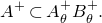 $ A^+\subset A_\theta^+ B_\theta^+.$
The space
$ A^+\subset A_\theta^+ B_\theta^+.$
The space $\mathfrak a_\theta^*=\operatorname{Hom}(\mathfrak a_\theta, \mathbb R)$
can be identified with the subspace of
$\mathfrak a_\theta^*=\operatorname{Hom}(\mathfrak a_\theta, \mathbb R)$
can be identified with the subspace of $\mathfrak a^*$
consisting of
$\mathfrak a^*$
consisting of $p_\theta$
-invariant linear forms:
$p_\theta$
-invariant linear forms:
 \begin{equation}\mathfrak a_\theta^*=\{\psi\in \mathfrak a^*: \psi\circ p_\theta=\psi\}.\end{equation}
Hence, for $\theta_1\subset \theta_2$
, we have
$\theta_1\subset \theta_2$
, we have
 \begin{equation}\mathfrak a_{\theta_1}^*\subset \mathfrak a_{\theta_2}^*.\end{equation}
When $\theta=\Pi$
, we will omit the subscript. So
$\theta=\Pi$
, we will omit the subscript. So $P=P_\Pi$
is a minimal parabolic subgroup and
$P=P_\Pi$
is a minimal parabolic subgroup and $P=MAN$
.
$P=MAN$
.
2.1 Cartan projection
Recall the Cartan decomposition $G = KA^+ K$
, which means that for every
$G = KA^+ K$
, which means that for every $g\in G$
, there exists a unique element
$g\in G$
, there exists a unique element $\mu(g)\in \mathfrak a^+$
such that
$\mu(g)\in \mathfrak a^+$
such that $g\in K \exp \mu(g) K$
. The map
$g\in K \exp \mu(g) K$
. The map $G\to \mathfrak a^+$
given by
$G\to \mathfrak a^+$
given by $g\mapsto \mu(g)$
is called the Cartan projection. We have
$g\mapsto \mu(g)$
is called the Cartan projection. We have
 \begin{equation}\mu(g^{-1})={\rm i} (\mu(g))\quad\text{for all $g\in G$. }\end{equation}
Let $X = G/K$
be the associated Riemannian symmetric space and set
$X = G/K$
be the associated Riemannian symmetric space and set $o = [K] \in X$
. Fix a K-invariant norm
$o = [K] \in X$
. Fix a K-invariant norm $\| \cdot \|$
on
$\| \cdot \|$
on $\mathfrak g$
and a Riemannian distance d on X, induced from the Killing form on
$\mathfrak g$
and a Riemannian distance d on X, induced from the Killing form on $\mathfrak g$
, so that
$\mathfrak g$
, so that
 $$d(go, ho)=\|\mu(g^{-1}h)\|$$
for any $g, h \in G$
. For
$g, h \in G$
. For $p \in X$
and
$p \in X$
and $R \gt 0$
, let B(p, R) denote the metric ball
$R \gt 0$
, let B(p, R) denote the metric ball $ \{x \in X : d(x, p) \lt R\}$
.
$ \{x \in X : d(x, p) \lt R\}$
.
Lemma 2.1 [Reference BenoistBen97, Lemma 4.6]. For any compact subset $Q \subset G$
, there exists a constant
$Q \subset G$
, there exists a constant $C=C_Q\gt 0$
such that for all
$C=C_Q\gt 0$
such that for all $g \in G$
,
$g \in G$
,
 $$\sup_{q_1, q_2\in Q} \| \mu(q_1gq_2) -\mu(g)\| \lt C .$$
We then write
 $$\mu_{\theta} := p_{\theta} \circ \mu :G\to \mathfrak a_\theta^+.$$
In view of (2.3), we have $\psi\circ \mu_\theta=\psi \circ \mu$
for all
$\psi\circ \mu_\theta=\psi \circ \mu$
for all $\psi\in \mathfrak a_\theta^*$
.
$\psi\in \mathfrak a_\theta^*$
.
2.2 The
$\theta$
-boundary
$\mathcal F_\theta$


We set
 $$\mathcal F_\theta=G/P_{\theta} \quad\text{and}\quad \mathcal F=G/P.$$
Let
 $$ \pi_\theta:\mathcal F\to \mathcal F_\theta$$
denote the canonical projection map given by $gP\mapsto gP_\theta$
,
$gP\mapsto gP_\theta$
, $g\in G$
. We set
$g\in G$
. We set
 \begin{equation} \xi_\theta=[P_\theta] \in \mathcal F_{\theta}.\end{equation}
By the Iwasawa decomposition $G=KP=KAN$
, the subgroup K acts transitively on
$G=KP=KAN$
, the subgroup K acts transitively on $\mathcal F_\theta$
, and hence
$\mathcal F_\theta$
, and hence $\mathcal F_\theta\simeq K/ M_\theta.$
We consider the following notion of convergence of a sequence in G (or in X) to an element of $\mathcal F_\theta$
. For a sequence
$\mathcal F_\theta$
. For a sequence $g_i \in G$
, we say
$g_i \in G$
, we say $g_i \to \infty$ $\theta$
-regularly if
$\theta$
-regularly if $\min_{\alpha\in \theta} \alpha(\mu(g_i)) \to \infty$
as
$\min_{\alpha\in \theta} \alpha(\mu(g_i)) \to \infty$
as $i \to \infty$
.
$i \to \infty$
.
Definition 2.2. For a sequence $g_i\in G$
and
$g_i\in G$
and $\xi\in \mathcal F_\theta$
, we write
$\xi\in \mathcal F_\theta$
, we write $\lim_{i\to \infty} g_i=\lim g_i o =\xi$
and say
$\lim_{i\to \infty} g_i=\lim g_i o =\xi$
and say $g_i $
(or
$g_i $
(or $g_io \in X$
) converges to
$g_io \in X$
) converges to $\xi$
if:
$\xi$
if:
-
–
$g_i \to \infty$
$\theta$
-regularly; and -
–
$\lim_{i\to\infty} \kappa_{i}\xi_\theta= \xi$
in
$\mathcal F_\theta$
for some
$\kappa_{i}\in K$
such that
$g_i\in \kappa_{i} A^+ K$
.





2.3 Points in general position
Let $P_\theta^+$
be the standard parabolic subgroup of G opposite to
$P_\theta^+$
be the standard parabolic subgroup of G opposite to $P_\theta$
such that
$P_\theta$
such that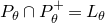 $P_\theta\cap P_\theta^+=L_\theta$
. We have
$P_\theta\cap P_\theta^+=L_\theta$
. We have $P_\theta^+ =w_0 P_{{\rm i}(\theta)}w_0^{-1}$
and hence
$P_\theta^+ =w_0 P_{{\rm i}(\theta)}w_0^{-1}$
and hence
 $$\mathcal F_{{\rm i}(\theta)}=G/P_\theta^+.$$
For $g\in G$
, we set
$g\in G$
, we set
 $$g_\theta^+ := gP_{\theta}\quad \text{and}\quad g_\theta^- := g w_0 P_{{\rm i}(\theta)};$$
as we fix $\theta$
in the entire paper, we write
$\theta$
in the entire paper, we write $g^{\pm}=g_\theta^{\pm}$
for simplicity when there is no room for confusion. Hence, for the identity
$g^{\pm}=g_\theta^{\pm}$
for simplicity when there is no room for confusion. Hence, for the identity $e\in G$
,
$e\in G$
, $(e^+, e^-)=(P_\theta, P_\theta^+)=(\xi_\theta, w_0\xi_{{\rm i}(\theta)})$
. The G-orbit of
$(e^+, e^-)=(P_\theta, P_\theta^+)=(\xi_\theta, w_0\xi_{{\rm i}(\theta)})$
. The G-orbit of $(e^+, e^-)$
is the unique open G-orbit in
$(e^+, e^-)$
is the unique open G-orbit in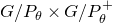 $G/P_\theta\times G/P_\theta^+$
under the diagonal G-action. We set
$G/P_\theta\times G/P_\theta^+$
under the diagonal G-action. We set
 \begin{equation} \mathcal F_{\theta}^{(2)}= \{(g_\theta^+, g_\theta^-): g\in G\}.\end{equation}
Two elements $\xi\in \mathcal F_\theta$
and
$\xi\in \mathcal F_\theta$
and $\eta\in \mathcal F_{{\rm i}(\theta)}$
are said to be in general position (or antipodal) if
$\eta\in \mathcal F_{{\rm i}(\theta)}$
are said to be in general position (or antipodal) if $(\xi, \eta)\in \mathcal F_\theta^{(2)}$
.
$(\xi, \eta)\in \mathcal F_\theta^{(2)}$
.
2.4 Busemann maps and Gromov products
The $\mathfrak a$
-valued Busemann map
$\mathfrak a$
-valued Busemann map $\beta: \mathcal F\times G \times G \to\mathfrak a $
is defined as follows: for
$\beta: \mathcal F\times G \times G \to\mathfrak a $
is defined as follows: for $\xi\in \mathcal F$
and
$\xi\in \mathcal F$
and $g, h\in G$
,
$g, h\in G$
,
 $$ \beta_\xi ( g, h):=\sigma (g^{-1}, \xi)-\sigma(h^{-1}, \xi)$$
where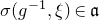 $\sigma(g^{-1},\xi)\in \mathfrak a$
is the unique element such that
$\sigma(g^{-1},\xi)\in \mathfrak a$
is the unique element such that $g^{-1}k \in K \exp (\sigma(g^{-1}, \xi)) N$
for any
$g^{-1}k \in K \exp (\sigma(g^{-1}, \xi)) N$
for any $k\in K$
with
$k\in K$
with $\xi=kP$
. For
$\xi=kP$
. For $(\xi,g,h)\in \mathcal F_\theta\times G\times G$
, we define
$(\xi,g,h)\in \mathcal F_\theta\times G\times G$
, we define
 \begin{equation} \beta_{\xi}^\theta (g, h): =p_\theta ( \beta_{\xi_0} (g, h)) \quad\text{for $\xi_0\in \pi_\theta^{-1}(\xi)$};\end{equation}
this is well-defined independent of the choice of $\xi_0$
(see [Reference QuintQui02b, Lemma 6.1]). We also have
$\xi_0$
(see [Reference QuintQui02b, Lemma 6.1]). We also have $\|\beta_\xi^{\theta}(g, h)\|\le d(go, ho)$
for all
$\|\beta_\xi^{\theta}(g, h)\|\le d(go, ho)$
for all $g, h\in G$
(see [Reference QuintQui02b, Lemma 8.9]). The Busemann map has the following properties: for all
$g, h\in G$
(see [Reference QuintQui02b, Lemma 8.9]). The Busemann map has the following properties: for all $\xi \in \mathcal F_{\theta}$
and
$\xi \in \mathcal F_{\theta}$
and $g_1, g_2, g_3\in G$
,
$g_1, g_2, g_3\in G$
,
 $$\begin{aligned} \text{(Invariance)} \quad & \beta_{\xi}^{\theta}(g_1, g_2) = \beta_{g_3 \xi}^{\theta}(g_3 g_1, g_3 g_2);\\ \text{(Cocycle property)} \quad & \beta_{\xi}^{\theta}(g_1, g_2) = \beta_{\xi}^{\theta}(g_1, g_3) + \beta_{\xi}^{\theta}(g_3, g_2).\end{aligned}$$
For $p, q \in X$
and
$p, q \in X$
and $\xi \in \mathcal F_{\theta}$
, we set
$\xi \in \mathcal F_{\theta}$
, we set $\beta_{\xi}^{\theta}(p, q) := \beta_{\xi}^{\theta}(g, h)$
where
$\beta_{\xi}^{\theta}(p, q) := \beta_{\xi}^{\theta}(g, h)$
where $g, h \in G$
satisfies
$g, h \in G$
satisfies $go = p$
and
$go = p$
and $ho=q$
. It is easy to check that this is well-defined.
$ho=q$
. It is easy to check that this is well-defined.
Definition 2.3.
For $(\xi, \eta) \in \mathcal F_{\theta}^{(2)}$
, we define the
$(\xi, \eta) \in \mathcal F_{\theta}^{(2)}$
, we define the $\theta$
-Gromov product as
$\theta$
-Gromov product as
 $$\mathcal G^{\theta}(\xi, \eta) = \tfrac{1}{2} ( \beta_{\xi}^{\theta}(e, g) + {\rm i} (\beta_{\eta}^{{\rm i}(\theta)}(e, g))),$$
where $g \in G$
satisfies
$g \in G$
satisfies $(g^+, g^-) = (\xi, \eta)$
. This does not depend on the choice of g (see [Reference Kim, Oh and WangKOW25b, Lemma 9.11]).
$(g^+, g^-) = (\xi, \eta)$
. This does not depend on the choice of g (see [Reference Kim, Oh and WangKOW25b, Lemma 9.11]).
3. Classification of Patterson–Sullivan measures by tangent forms
Let G be a connected semisimple real algebraic group. We fix a non-empty subset $\theta$
of the set
$\theta$
of the set $\Pi$
of all simple roots. Throughout this section, let
$\Pi$
of all simple roots. Throughout this section, let $\Gamma$
be a discrete subgroup of G. When
$\Gamma$
be a discrete subgroup of G. When $\Gamma$
is
$\Gamma$
is $\theta$
-Anosov, we have a complete classification of all linear forms
$\theta$
-Anosov, we have a complete classification of all linear forms $\psi\in \mathfrak a_\theta^*$
admitting a
$\psi\in \mathfrak a_\theta^*$
admitting a $(\Gamma, \psi)$
-Patterson–Sullivan measure [Reference Lee and OhLO23, Reference SambarinoSam24, Reference Kim, Oh and WangKOW25b]. The goal of this section is to review this classification, in addition to recalling some basic notions such as the limit cone and the growth indicator of
$(\Gamma, \psi)$
-Patterson–Sullivan measure [Reference Lee and OhLO23, Reference SambarinoSam24, Reference Kim, Oh and WangKOW25b]. The goal of this section is to review this classification, in addition to recalling some basic notions such as the limit cone and the growth indicator of $\Gamma$
. For a more detailed discussion of the material of this section, we refer to [Reference Kim, Oh and WangKOW25b].
$\Gamma$
. For a more detailed discussion of the material of this section, we refer to [Reference Kim, Oh and WangKOW25b].
The $\theta$
-limit set of
$\theta$
-limit set of $\Gamma$
is defined as follows:
$\Gamma$
is defined as follows:
 $$\Lambda_{\theta}=\Lambda_{\theta}(\Gamma):=\{\lim {\gamma}_i\in \mathcal F_\theta:\ {\gamma}_i\in \Gamma \},$$
where $\lim \gamma_i$
is defined as in Definition 2.2. If
$\lim \gamma_i$
is defined as in Definition 2.2. If $\Gamma \lt G$
is Zariski dense, then the limit set
$\Gamma \lt G$
is Zariski dense, then the limit set $\Lambda_{\theta}$
is the unique
$\Lambda_{\theta}$
is the unique $\Gamma$
-minimal subset of
$\Gamma$
-minimal subset of $\mathcal F_{\theta}$
(see [Reference BenoistBen97, § 3.6] and [Reference QuintQui02b, Theorem 7.2]). Furthermore, if we set
$\mathcal F_{\theta}$
(see [Reference BenoistBen97, § 3.6] and [Reference QuintQui02b, Theorem 7.2]). Furthermore, if we set $\Lambda=\Lambda_\Pi$
, then
$\Lambda=\Lambda_\Pi$
, then $ \pi_{\theta}(\Lambda) = \Lambda_{\theta}$
. For
$ \pi_{\theta}(\Lambda) = \Lambda_{\theta}$
. For $\psi \in \mathfrak a_{\theta}^*$
, a Borel probability measure
$\psi \in \mathfrak a_{\theta}^*$
, a Borel probability measure $\nu$
on
$\nu$
on $\mathcal F_{\theta}$
is called a
$\mathcal F_{\theta}$
is called a $(\Gamma, \psi)$
-conformal measure if for all
$(\Gamma, \psi)$
-conformal measure if for all $\gamma \in \Gamma$
and
$\gamma \in \Gamma$
and $\xi \in \mathcal F_{\theta}$
,
$\xi \in \mathcal F_{\theta}$
,
 $$\frac{d \gamma_* \nu}{d \nu}(\xi) = e^{\psi(\beta_{\xi}^{\theta}(e, \gamma))},$$
where $\gamma_*\nu(B) = \nu(\gamma^{-1} B)$
for any Borel
$\gamma_*\nu(B) = \nu(\gamma^{-1} B)$
for any Borel $B \subset \mathcal F_{\theta}$
. A
$B \subset \mathcal F_{\theta}$
. A $(\Gamma, \psi)$
-conformal measure is called a
$(\Gamma, \psi)$
-conformal measure is called a $(\Gamma, \psi)$
-Patterson–Sullivan measure if it is supported on
$(\Gamma, \psi)$
-Patterson–Sullivan measure if it is supported on $\Lambda_{\theta}$
.
$\Lambda_{\theta}$
.
In order to discuss which linear forms $\psi$
admit a Patterson–Sullivan measure, we need the definitions of the
$\psi$
admit a Patterson–Sullivan measure, we need the definitions of the $\theta$
-limit cones and growth indicators.
$\theta$
-limit cones and growth indicators.
The $\theta$
-limit cone
$\theta$
-limit cone $\mathcal L_{\theta}=\mathcal L_\theta(\Gamma)$
of
$\mathcal L_{\theta}=\mathcal L_\theta(\Gamma)$
of $\Gamma$
is defined as the asymptotic cone of
$\Gamma$
is defined as the asymptotic cone of $\mu_{\theta}(\Gamma)$
in
$\mu_{\theta}(\Gamma)$
in $\mathfrak a_{\theta}$
; that is,
$\mathfrak a_{\theta}$
; that is, $u\in \mathcal L_\theta$
if and only if
$u\in \mathcal L_\theta$
if and only if $u=\lim t_i \mu_\theta(\gamma_i)$
for some sequences
$u=\lim t_i \mu_\theta(\gamma_i)$
for some sequences $t_i\to 0$
and
$t_i\to 0$
and $\gamma_i\in \Gamma$
. If
$\gamma_i\in \Gamma$
. If $\Gamma$
is Zariski dense,
$\Gamma$
is Zariski dense, $\mathcal L_\theta$
is a convex cone with non-empty interior by [Reference BenoistBen97, § 1.2]. Recalling the convention of dropping the subscript
$\mathcal L_\theta$
is a convex cone with non-empty interior by [Reference BenoistBen97, § 1.2]. Recalling the convention of dropping the subscript $\theta$
when
$\theta$
when $\theta=\Pi$
, we write
$\theta=\Pi$
, we write $\mathcal L=\mathcal L_\Pi$
. We then have
$\mathcal L=\mathcal L_\Pi$
. We then have $p_\theta(\mathcal L)=\mathcal L_\theta$
.
$p_\theta(\mathcal L)=\mathcal L_\theta$
.
3.1 Growth indicators
We say that $\Gamma$
is
$\Gamma$
is $\theta$
-discrete if the restriction
$\theta$
-discrete if the restriction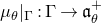 $\mu_\theta|_{\Gamma}:\Gamma \to \mathfrak a_\theta^+$
is proper. The
$\mu_\theta|_{\Gamma}:\Gamma \to \mathfrak a_\theta^+$
is proper. The $\theta$
-discreteness of
$\theta$
-discreteness of $\Gamma$
implies that
$\Gamma$
implies that $\mu_\theta(\Gamma)$
is a closed discrete subset of
$\mu_\theta(\Gamma)$
is a closed discrete subset of $\mathfrak a_\theta^+$
. Indeed,
$\mathfrak a_\theta^+$
. Indeed, $\Gamma$
is
$\Gamma$
is $\theta$
-discrete if and only if the counting measure on
$\theta$
-discrete if and only if the counting measure on $\mu_\theta(\Gamma)$
weighted with multiplicity is a Radon measure on
$\mu_\theta(\Gamma)$
weighted with multiplicity is a Radon measure on $\mathfrak a_\theta^+$
.
$\mathfrak a_\theta^+$
.
Definition 3.1 ( $\theta$
-growth [Reference QuintQui02a, Reference Kim, Oh and WangKOW25b]). For a
$\theta$
-growth [Reference QuintQui02a, Reference Kim, Oh and WangKOW25b]). For a $\theta$
-discrete subgroup
$\theta$
-discrete subgroup $\Gamma\lt G$
, the
$\Gamma\lt G$
, the $\theta$
-growth indicator
$\theta$
-growth indicator $\psi_\Gamma^{\theta}:\mathfrak a_\theta\to [-\infty, \infty] $
is defined as follows: if
$\psi_\Gamma^{\theta}:\mathfrak a_\theta\to [-\infty, \infty] $
is defined as follows: if $u \in \mathfrak a_\theta$
is non-zero,
$u \in \mathfrak a_\theta$
is non-zero,
 \begin{equation} \psi_\Gamma^{\theta}(u)=\|u\| \inf_{u\in \mathcal C}\tau^\theta_{\mathcal C},\end{equation}
where $\mathcal C\subset \mathfrak a_\theta$
ranges over all open cones containing u, and
$\mathcal C\subset \mathfrak a_\theta$
ranges over all open cones containing u, and $\psi_{\Gamma}^{\theta}(0) = 0$
. Here,
$\psi_{\Gamma}^{\theta}(0) = 0$
. Here, $-\infty\le \tau^{\theta}_{\mathcal C}\le \infty$
denotes the abscissa of convergence of the series
$-\infty\le \tau^{\theta}_{\mathcal C}\le \infty$
denotes the abscissa of convergence of the series ${\mathcal P}^{\theta}_{\mathcal C}(s)=\sum_{\gamma\in \Gamma, \mu_\theta(\gamma)\in \mathcal C} e^{-s\|\mu_\theta(\gamma)\|}$
. As mentioned, we simply write
${\mathcal P}^{\theta}_{\mathcal C}(s)=\sum_{\gamma\in \Gamma, \mu_\theta(\gamma)\in \mathcal C} e^{-s\|\mu_\theta(\gamma)\|}$
. As mentioned, we simply write $\psi_{\Gamma} := \psi_{\Gamma}^{\Pi}$
.
$\psi_{\Gamma} := \psi_{\Gamma}^{\Pi}$
.
This definition is independent of the choice of a norm on $\mathfrak a_\theta$
. It has been proved in [Reference QuintQui02a, Theorem 1.1.1] and [Reference Kim, Oh and WangKOW25b, Theorem 3.3] that
$\mathfrak a_\theta$
. It has been proved in [Reference QuintQui02a, Theorem 1.1.1] and [Reference Kim, Oh and WangKOW25b, Theorem 3.3] that
 $$\psi_{\Gamma}^{\theta} \lt \infty, \quad \mathcal L_{\theta} = \{\psi_{\Gamma}^{\theta} \ge 0\}\quad \text{and } \quad \psi_{\Gamma}^{\theta} \gt 0\; \text{on}\operatorname{{\rm int}} \mathcal L_{\theta},$$
where $\operatorname{{\rm int}}\mathcal L_\theta$
denotes the interior of
$\operatorname{{\rm int}}\mathcal L_\theta$
denotes the interior of $\mathcal L_\theta$
in the relative topology of
$\mathcal L_\theta$
in the relative topology of $\mathfrak a_{\theta}$
. Moreover,
$\mathfrak a_{\theta}$
. Moreover, $\psi_\Gamma^\theta$
is upper semi-continuous and concave. When
$\psi_\Gamma^\theta$
is upper semi-continuous and concave. When $\theta={\rm i}(\theta)$
, it follows from (2.5) that
$\theta={\rm i}(\theta)$
, it follows from (2.5) that $\psi_\Gamma^\theta$
is i-invariant.
$\psi_\Gamma^\theta$
is i-invariant.
We say that a linear form $\psi$
is tangent to
$\psi$
is tangent to $\psi_\Gamma^\theta$
(at
$\psi_\Gamma^\theta$
(at $u\in \mathfrak a_\theta-\{0\}$
) if
$u\in \mathfrak a_\theta-\{0\}$
) if $\psi\ge \psi_\Gamma^\theta$
and
$\psi\ge \psi_\Gamma^\theta$
and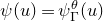 $\psi(u)=\psi_\Gamma^\theta(u)$
. For any
$\psi(u)=\psi_\Gamma^\theta(u)$
. For any $u\in \operatorname{{\rm int}} \mathcal L_\theta$
, there exists
$u\in \operatorname{{\rm int}} \mathcal L_\theta$
, there exists $\psi\in \mathfrak a_\theta^*$
tangent to
$\psi\in \mathfrak a_\theta^*$
tangent to $\psi_\Gamma^\theta$
at u. Moreover, for any
$\psi_\Gamma^\theta$
at u. Moreover, for any $\psi\in \mathfrak a_\theta^*$
tangent to
$\psi\in \mathfrak a_\theta^*$
tangent to $\psi_\Gamma^\theta$
at an interior direction of
$\psi_\Gamma^\theta$
at an interior direction of $\mathfrak a_\theta^+$
, there exists a
$\mathfrak a_\theta^+$
, there exists a $(\Gamma, \psi)$
-Patterson–Sullivan measure (see [Reference QuintQui02b, Theorem 8.4] and [Reference Kim, Oh and WangKOW25b, Proposition 5.9]).
$(\Gamma, \psi)$
-Patterson–Sullivan measure (see [Reference QuintQui02b, Theorem 8.4] and [Reference Kim, Oh and WangKOW25b, Proposition 5.9]).
For $\theta$
-Anosov subgroups, we have a more precise classification of Patterson–Sullivan measures in terms of tangent forms.
$\theta$
-Anosov subgroups, we have a more precise classification of Patterson–Sullivan measures in terms of tangent forms.
Definition 3.2
A finitely generated subgroup $\Gamma\lt G$
is
$\Gamma\lt G$
is $\theta$
-Anosov if there exists a constant
$\theta$
-Anosov if there exists a constant $C \gt 1$
such that for all
$C \gt 1$
such that for all $\alpha \in \theta$
and
$\alpha \in \theta$
and $\gamma\in \Gamma$
, we have
$\gamma\in \Gamma$
, we have
 \begin{equation} \alpha(\mu(\gamma)) \ge C^{-1} |\gamma| - C,\end{equation}
where $|\cdot|$
denotes a fixed word metric on
$|\cdot|$
denotes a fixed word metric on $\Gamma$
.
$\Gamma$
.
We recall that all $\theta$
-Anosov subgroups are assumed to be non-elementary in this paper. Define
$\theta$
-Anosov subgroups are assumed to be non-elementary in this paper. Define
 \begin{equation} \mathscr T_\Gamma=\{\psi\in \mathfrak a_\theta^*:\text{$\psi$ is tangent to $\psi_\Gamma^\theta$} \} .\end{equation}
By the duality lemma (see [Reference QuintQui03a, § 4] and [Reference SambarinoSam14, Lemma 4.8]), the following can be deduced from [Reference SambarinoSam24, Theorem A] (see [Reference Kim, Oh and WangKOW25b, Theorem 13.2]).
Theorem 3.3.
Let $\Gamma$
be a
$\Gamma$
be a $\theta$
-Anosov subgroup.
$\theta$
-Anosov subgroup.
-
(1) We then have that
$\psi_\Gamma^\theta$
is analytic on
$\operatorname{{\rm int}} \mathcal L_{\theta}$
, strictly concave on
$\mathcal L_{\theta}$
, and vertically tangent.Footnote
5
-
(2) For any
$\psi \in \mathscr T_\Gamma$
, there exists a unique unit vector
$u=u_\psi\in \operatorname{{\rm int}} \mathcal L_\theta$
such that
$\psi(u)=\psi_\Gamma^\theta(u)$
. If
$\Gamma$
is Zariski dense, the map
$\psi\mapsto u_\psi$
is a bijection between
$\mathscr T_\Gamma$
and
$\{u\in \operatorname{{\rm int}} \mathcal L_{\theta}:\|u\|=1\}$
.



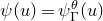



The following theorem has been proved in [Reference Lee and OhLO23, Theorem 1.3] for $\theta=\Pi$
and
$\theta=\Pi$
and $\Gamma$
Zariski dense. The general case follows from [Reference SambarinoSam24, Theorem A] (for a more general discussion on conformal measures, see [Reference Kim, Oh and WangKOW25b, Corollary 1.13]).
$\Gamma$
Zariski dense. The general case follows from [Reference SambarinoSam24, Theorem A] (for a more general discussion on conformal measures, see [Reference Kim, Oh and WangKOW25b, Corollary 1.13]).
Theorem 3.4.
Let $\Gamma$
be a
$\Gamma$
be a $\theta$
-Anosov subgroup. For any
$\theta$
-Anosov subgroup. For any $\psi\in \mathscr T_\Gamma$
, there exists a unique
$\psi\in \mathscr T_\Gamma$
, there exists a unique $(\Gamma, \psi)$
-Patterson–Sullivan measure on
$(\Gamma, \psi)$
-Patterson–Sullivan measure on $\Lambda_\theta$
, which we denote by
$\Lambda_\theta$
, which we denote by $\nu_\psi=\nu_{\psi, \theta}$
. The map
$\nu_\psi=\nu_{\psi, \theta}$
. The map
 $$\psi\mapsto \nu_\psi$$
is a surjection from $\mathscr T_\Gamma$
to the space of all
$\mathscr T_\Gamma$
to the space of all $\Gamma$
-Patterson–Sullivan measures. If
$\Gamma$
-Patterson–Sullivan measures. If $\Gamma$
is Zariski dense, then the map
$\Gamma$
is Zariski dense, then the map $\psi \mapsto \nu_{\psi}$
is bijective. Moreover, if
$\psi \mapsto \nu_{\psi}$
is bijective. Moreover, if $\psi_1\ne \psi_2$
in
$\psi_1\ne \psi_2$
in $\mathscr T_\Gamma$
, then
$\mathscr T_\Gamma$
, then $\nu_{\psi_1}$
and
$\nu_{\psi_1}$
and $\nu_{\psi_2}$
are mutually singular to each other.
$\nu_{\psi_2}$
are mutually singular to each other.
Remark 3.5. One immediate consequence of the last statement of Theorem 3.4 is that at most one Patterson–Sullivan measure can be a Hausdorff measure on $\Lambda_\theta$
with respect to a fixed metric (e.g., Riemannian metric).
$\Lambda_\theta$
with respect to a fixed metric (e.g., Riemannian metric).
When $\psi\in \mathfrak a_\theta^*$
is positive on
$\psi\in \mathfrak a_\theta^*$
is positive on $\mathcal L_{\theta}-\{0\}$
, the abscissa of convergence of the
$\mathcal L_{\theta}-\{0\}$
, the abscissa of convergence of the $\psi$
-Poincaré series
$\psi$
-Poincaré series
 $$s \mapsto \sum_{\gamma \in \Gamma} e^{-s \psi(\mu(\gamma))}$$
is a well-defined positive number, which we denote by $\delta_\psi$
(see [Reference Kim, Oh and WangKOW25b, Lemma 4.3]). Equivalently,
$\delta_\psi$
(see [Reference Kim, Oh and WangKOW25b, Lemma 4.3]). Equivalently, $\delta_\psi$
is also given by (1.3).
$\delta_\psi$
is also given by (1.3).
Lemma 3.6 [Reference Kim, Oh and WangKOW25b, Lemma 4.5]. If $\psi\in \mathfrak a_\theta^*$
is positive on
$\psi\in \mathfrak a_\theta^*$
is positive on $\mathcal L_\theta-\{0\}$
, then
$\mathcal L_\theta-\{0\}$
, then
 $$\delta_\psi \psi \in \mathscr T_\Gamma .$$
In particular, $\psi \in \mathscr T_{\Gamma}$
if and only if
$\psi \in \mathscr T_{\Gamma}$
if and only if $\delta_{\psi} = 1$
.
$\delta_{\psi} = 1$
.
Since $\mu(g^{-1}) = {\rm i}(\mu(g))$
for all
$\mu(g^{-1}) = {\rm i}(\mu(g))$
for all $g \in G$
, we have that
$g \in G$
, we have that $\Gamma$
is
$\Gamma$
is $\theta$
-Anosov if and only if
$\theta$
-Anosov if and only if $\Gamma$
is
$\Gamma$
is $\theta \cup {\rm i}(\theta)$
-Anosov. If
$\theta \cup {\rm i}(\theta)$
-Anosov. If $\Gamma$
is
$\Gamma$
is $\theta$
-Anosov, then the canonical projection map
$\theta$
-Anosov, then the canonical projection map $p:\Lambda_{\theta \cup {\rm i}(\theta)} \to \Lambda_{\theta}$
is a
$p:\Lambda_{\theta \cup {\rm i}(\theta)} \to \Lambda_{\theta}$
is a $\Gamma$
-equivariant homeomorphism. Recalling that
$\Gamma$
-equivariant homeomorphism. Recalling that $\mathfrak a_\theta^*$
can be considered as a subset of
$\mathfrak a_\theta^*$
can be considered as a subset of $\mathfrak a_{\theta\cup{\rm i}(\theta)}^*$
from (2.4), we recall the following, which will be of use.
$\mathfrak a_{\theta\cup{\rm i}(\theta)}^*$
from (2.4), we recall the following, which will be of use.
Lemma 3.7 [Reference Kim, Oh and WangKOW25b, Lemma 9.5]. Let $\Gamma$
be a
$\Gamma$
be a $\theta$
-Anosov subgroup. For any
$\theta$
-Anosov subgroup. For any $\psi \in \mathscr T_\Gamma$
, the measure
$\psi \in \mathscr T_\Gamma$
, the measure $\nu_{\psi,\theta}$
coincides with the push-forward of
$\nu_{\psi,\theta}$
coincides with the push-forward of $\nu_{\psi, \theta\cup{\rm i}(\theta)}$
by p.
$\nu_{\psi, \theta\cup{\rm i}(\theta)}$
by p.
3.2 Gromov hyperbolic space and quasi-isometry
We collect a few basic facts about $\theta$
-Anosov subgroups that will be used repeatedly.
$\theta$
-Anosov subgroups that will be used repeatedly.
Recall that a geodesic metric spaceFootnote
6 $(Z, d_Z)$
is called a Gromov hyperbolic space if it satisfies a uniformly thin-triangle property; that is, there exists
$(Z, d_Z)$
is called a Gromov hyperbolic space if it satisfies a uniformly thin-triangle property; that is, there exists $T \gt 0$
such that for any geodesic triangle in Z, one side of the triangle is contained in the T-neighborhood of the union of two other sides. We denote by
$T \gt 0$
such that for any geodesic triangle in Z, one side of the triangle is contained in the T-neighborhood of the union of two other sides. We denote by $\partial Z$
the Gromov boundary of Z, which is the space of equivalence classes of geodesic rays in Z. For any
$\partial Z$
the Gromov boundary of Z, which is the space of equivalence classes of geodesic rays in Z. For any $z_1\ne z_2\in Z\cup \partial Z$
, there may be more than one geodesic connecting
$z_1\ne z_2\in Z\cup \partial Z$
, there may be more than one geodesic connecting $z_1$
and
$z_1$
and $z_2$
. By the notation
$z_2$
. By the notation $[z_1, z_2]$
, we mean ‘a’ geodesic in Z connecting
$[z_1, z_2]$
, we mean ‘a’ geodesic in Z connecting $z_1$
to
$z_1$
to $z_2$
. For
$z_2$
. For $w\in Z$
, the nearest-point projection of w to a geodesic
$w\in Z$
, the nearest-point projection of w to a geodesic $[z_1,z_2]$
is any point
$[z_1,z_2]$
is any point $w'\in [z_1, z_2]$
satisfying
$w'\in [z_1, z_2]$
satisfying $d_Z(w,w')=\inf \{d_Z(w, z):z\in [z_1, z_2]\}$
. This is coarsely well-defined. We refer to [Reference Bridson and HaefligerBH99] for basics on Gromov hyperbolic spaces. Recall that d denotes the Riemannian distance function on
$d_Z(w,w')=\inf \{d_Z(w, z):z\in [z_1, z_2]\}$
. This is coarsely well-defined. We refer to [Reference Bridson and HaefligerBH99] for basics on Gromov hyperbolic spaces. Recall that d denotes the Riemannian distance function on $X=G/K$
.
$X=G/K$
.
Theorem 3.8 (See [Reference Kapovich, Leeb and PortiKLP18, Corollary 1.6] and [Reference Kapovich, Leeb and PortiKLP17, Proposition 5.16, Lemma 5.23]; see also [Reference Guéritaud, Guichard, Kassel and WienhardGGK+17]). Let $\Gamma$
be a
$\Gamma$
be a $\theta$
-Anosov subgroup. Fix a word metric
$\theta$
-Anosov subgroup. Fix a word metric $\mathsf{d}_\Gamma$
on
$\mathsf{d}_\Gamma$
on $\Gamma$
with respect to a finite symmetric generating set.
$\Gamma$
with respect to a finite symmetric generating set.
-
(1) We have that
$(\Gamma, \mathsf{d}_\Gamma)$
is a Gromov hyperbolic space.Footnote
7
-
(2) Then,
$\mathcal L_\theta-\{0\}$
is contained in the relative interior of
$\mathfrak a_\theta^+$
in
$\mathfrak a_\theta$
. -
(3) The orbit map
$ (\Gamma,\mathsf{d}_\Gamma) \to (\Gamma o, d)$
given by
$ \gamma \mapsto \gamma o $
is a quasi-isometric embedding, i.e., there exist
$Q=Q_\Gamma\ge 1$
such that for all
$\gamma_1, \gamma_2\in \Gamma$
,
$$ Q^{-1}\cdot \mathsf{d}_{\Gamma}(\gamma_1, \gamma_2) -Q \le d(\gamma_1 o, \gamma_2 o) \le Q \cdot \mathsf{d}_{\Gamma}(\gamma_1, \gamma_2) +Q .$$
-
(4) The orbit map
$\Gamma \to \Gamma o$
uniquely extends to a
$\Gamma$
-equivariant continuous map
$f:\Gamma \cup \partial \Gamma \to \Gamma o \cup \Lambda_{\theta}$
and
$f|_{\partial \Gamma}$
is a homeomorphism onto
$\Lambda_\theta$
. For
$\theta={\rm i}(\theta)$
, f maps two distinct points of
$\partial \Gamma$
to points in general position.








We henceforth identity $\partial \Gamma$
and
$\partial \Gamma$
and $\Lambda_\theta$
using f. For any
$\Lambda_\theta$
using f. For any $\xi\ne \eta \in \Gamma \cup \partial \Gamma$
, note that
$\xi\ne \eta \in \Gamma \cup \partial \Gamma$
, note that $f([\xi, \eta])=[\xi, \eta] o$
is the image of
$f([\xi, \eta])=[\xi, \eta] o$
is the image of $[\xi, \eta]$
under the orbit map.
$[\xi, \eta]$
under the orbit map.
4. Metric-like functions on
$\Gamma$
-orbits and diamonds

We fix a non-empty subset $\theta \subset \Pi$
. In this section, we assume that
$\theta \subset \Pi$
. In this section, we assume that $\theta$
is symmetric, i.e.,
$\theta$
is symmetric, i.e., $\theta = {\rm i}(\theta)$
. Recall the notation
$\theta = {\rm i}(\theta)$
. Recall the notation $X=G/K$
and
$X=G/K$
and $o=[K]\in X$
.
$o=[K]\in X$
.
For a linear form $\psi \in \mathfrak a_{\theta}^*$
, define
$\psi \in \mathfrak a_{\theta}^*$
, define $\mathsf{d}_{\psi} : X \times X \to \mathbb R$
as follows: for
$\mathsf{d}_{\psi} : X \times X \to \mathbb R$
as follows: for $g, h \in G$
,
$g, h \in G$
,
 \begin{equation} \mathsf{d}_{\psi}(g o, h o) :=\psi(\mu(g^{-1} h))=\psi(\mu_{\theta}(g^{-1} h)).\end{equation}
Since the Cartan projection $\mu$
is bi-K-invariant,
$\mu$
is bi-K-invariant, $\mathsf{d}_\psi$
is a well-defined left G-invariant function.
$\mathsf{d}_\psi$
is a well-defined left G-invariant function.
The main goal of this section is to prove the following theorem saying that when $\Gamma$
is
$\Gamma$
is $\theta$
-Anosov,
$\theta$
-Anosov, $\mathsf{d}_\psi$
behaves like a metric, restricted to the
$\mathsf{d}_\psi$
behaves like a metric, restricted to the $\Gamma$
-orbit
$\Gamma$
-orbit $\Gamma o$
for a proper class of
$\Gamma o$
for a proper class of $\psi$
values.
$\psi$
values.
Theorem 4.1 (Coarse triangle inequality) Let $\Gamma$
be a
$\Gamma$
be a $\theta$
-Anosov subgroup. Let
$\theta$
-Anosov subgroup. Let $\psi\in \mathfrak a_\theta^*$
be such that
$\psi\in \mathfrak a_\theta^*$
be such that $\psi\gt 0$
on
$\psi\gt 0$
on $\mathcal L_\theta-\{0\}$
. Then there exists a constant
$\mathcal L_\theta-\{0\}$
. Then there exists a constant $D=D_\psi\gt 0$
such that for all
$D=D_\psi\gt 0$
such that for all $\gamma_1, \gamma_2,\gamma \in \Gamma$
,
$\gamma_1, \gamma_2,\gamma \in \Gamma$
,
 $$\mathsf{d}_\psi(\gamma_1 o, \gamma_2 o)\le \mathsf{d}_\psi (\gamma_1 o, \gamma o)+\mathsf{d}_\psi (\gamma o, \gamma_2 o)+D.$$
Indeed, we prove Theorem 4.1 in a greater generality where the orbit $\Gamma o$
is replaced by the image of a uniformly regular quasi-isometric embedding of a geodesic metric space into X.
$\Gamma o$
is replaced by the image of a uniformly regular quasi-isometric embedding of a geodesic metric space into X.
4.1 Coarse triangle inequalities for uniformly regular quasi-isometric embeddings
We set $\mathcal W_\theta$
to be the set of all Weyl elements that fix
$\mathcal W_\theta$
to be the set of all Weyl elements that fix $\mathfrak a_\theta$
pointwise. We define a closed cone
$\mathfrak a_\theta$
pointwise. We define a closed cone $\mathcal C$
in
$\mathcal C$
in $\mathfrak a^+$
to be
$\mathfrak a^+$
to be $\theta$
-admissible if the following three conditions hold:
$\theta$
-admissible if the following three conditions hold:
-
(1)
$\mathcal C$
is i-invariant, so
${\rm i}(\mathcal C)=\mathcal C$
; -
(2)
$\mathcal W_\theta \cdot \mathcal C=\bigcup_{w\in \mathcal W_\theta} \operatorname{{\rm Ad}}_w \mathcal C $
is convex; and -
(3)
$\mathcal C\cap (\bigcup_{\alpha\in \theta} \ker \alpha) =\{0\}$
.




For a $\theta$
-admissible cone
$\theta$
-admissible cone $\mathcal C$
, we say that an ordered pair
$\mathcal C$
, we say that an ordered pair $(x_1, x_2)$
of distinct points in X is
$(x_1, x_2)$
of distinct points in X is $\mathcal C$
-regular if for
$\mathcal C$
-regular if for $g_1, g_2 \in G$
such that
$g_1, g_2 \in G$
such that $g_1 o = x_1$
and
$g_1 o = x_1$
and $g_2 o = x_2$
, we have
$g_2 o = x_2$
, we have
 $$\mu(g_1^{-1} g_2) \in \mathcal C.$$
In this case, $x_2 = g_2 o \in g_1 K (\exp \mathcal C) o$
and hence for some
$x_2 = g_2 o \in g_1 K (\exp \mathcal C) o$
and hence for some $g \in g_1 K$
,
$g \in g_1 K$
, $x_1 = g_1 o = go$
and
$x_1 = g_1 o = go$
and $x_2 \in g (\exp \mathcal C) o$
. Note that if
$x_2 \in g (\exp \mathcal C) o$
. Note that if $(x_1, x_2)$
is
$(x_1, x_2)$
is $\mathcal C$
-regular, then
$\mathcal C$
-regular, then $(x_2, x_1)$
is
$(x_2, x_1)$
is ${\rm i}(\mathcal C)$
-regular and hence
${\rm i}(\mathcal C)$
-regular and hence $\mathcal C$
-regular by the i-invariance of
$\mathcal C$
-regular by the i-invariance of $\mathcal C$
.
$\mathcal C$
.
Definition 4.2 Let $(Z, d_Z)$
be a metric space and
$(Z, d_Z)$
be a metric space and $f:Z\to X$
be a map. For a cone
$f:Z\to X$
be a map. For a cone $\mathcal C \subset \mathfrak a^+$
and a constant
$\mathcal C \subset \mathfrak a^+$
and a constant $B\ge 0$
, f is called
$B\ge 0$
, f is called $(\mathcal C,B)$
-regular if the pair
$(\mathcal C,B)$
-regular if the pair $(f(z_1),f(z_2))$
is
$(f(z_1),f(z_2))$
is $\mathcal C$
-regular for all
$\mathcal C$
-regular for all $z_1, z_2 \in Z$
with
$z_1, z_2 \in Z$
with $d_Z(z_1,z_2) \ge B$
. We simply say that f is
$d_Z(z_1,z_2) \ge B$
. We simply say that f is $\mathcal C$
-regular if it is
$\mathcal C$
-regular if it is $(\mathcal C, B)$
-regular for some
$(\mathcal C, B)$
-regular for some $B \ge 0$
.
$B \ge 0$
.
Theorem 4.1 will be deduced as a special case of the following theorem: we write $\mathcal C_\theta=p_\theta(\mathcal C)$
.
$\mathcal C_\theta=p_\theta(\mathcal C)$
.
Theorem 4.3.
Let Z be a geodesic metric space and $\mathcal C\subset \mathfrak a^+$
a
$\mathcal C\subset \mathfrak a^+$
a $\theta$
-admissible cone. Let
$\theta$
-admissible cone. Let $f: Z\to X$
be a
$f: Z\to X$
be a $\mathcal C$
-regular quasi-isometric embedding.
Footnote 8
If
$\mathcal C$
-regular quasi-isometric embedding.
Footnote 8
If $\psi \in \mathfrak a_\theta^*$
is positive on
$\psi \in \mathfrak a_\theta^*$
is positive on $\mathcal C -\{0\}$
, then there exists a constant
$\mathcal C -\{0\}$
, then there exists a constant $D=D_\psi \ge 0$
such that for all
$D=D_\psi \ge 0$
such that for all $x_1,x_2,x_3\in f(Z)$
,
$x_1,x_2,x_3\in f(Z)$
,
 \[ \mathsf{d}_\psi (x_1,x_3) \le \mathsf{d}_\psi (x_1,x_2) + \mathsf{d}_\psi (x_2,x_3) + D. \]
We continue to use notation $\operatorname{{\rm int}}\mathfrak a^+$
and
$\operatorname{{\rm int}}\mathfrak a^+$
and $\operatorname{{\rm int}}\mathfrak a_\theta^+$
for relative interiors in the topology of
$\operatorname{{\rm int}}\mathfrak a_\theta^+$
for relative interiors in the topology of $\mathfrak a$
and
$\mathfrak a$
and $\mathfrak a_\theta$
, respectively. Unless mentioned otherwise, for any proper cone
$\mathfrak a_\theta$
, respectively. Unless mentioned otherwise, for any proper cone $\mathcal C$
in
$\mathcal C$
in $\mathfrak a^+$
(respectively,
$\mathfrak a^+$
(respectively, $\mathfrak a_\theta^+$
), we denote by
$\mathfrak a_\theta^+$
), we denote by $\operatorname{{\rm int}} \mathcal C$
the interior of
$\operatorname{{\rm int}} \mathcal C$
the interior of $\mathcal C$
in the relative topology of
$\mathcal C$
in the relative topology of $\mathfrak a^+$
(respectively,
$\mathfrak a^+$
(respectively, $\mathfrak a_\theta^+$
).
$\mathfrak a_\theta^+$
).
4.2 Proof of Theorem 4.1 assuming Theorem 4.3
Let $\psi\in \mathfrak a_\theta^*$
be such that
$\psi\in \mathfrak a_\theta^*$
be such that $\psi\gt 0$
on
$\psi\gt 0$
on $\mathcal L_\theta-\{0\}$
. We will construct a
$\mathcal L_\theta-\{0\}$
. We will construct a $\theta$
-admissible cone
$\theta$
-admissible cone $\mathcal C\subset \mathfrak a^+$
such that
$\mathcal C\subset \mathfrak a^+$
such that $\mathcal L-\{0\}\subset \operatorname{{\rm int}} \mathcal C $
and
$\mathcal L-\{0\}\subset \operatorname{{\rm int}} \mathcal C $
and $\psi$
is positive on
$\psi$
is positive on $\mathcal C -\{0\}$
.
$\mathcal C -\{0\}$
.
Since $\theta={\rm i}(\theta)$
by hypothesis, it follows from (2.5) that
$\theta={\rm i}(\theta)$
by hypothesis, it follows from (2.5) that ${\rm i}|_{\mathfrak a_\theta}$
is an involution preserving
${\rm i}|_{\mathfrak a_\theta}$
is an involution preserving $\mathcal L_\theta$
. Since
$\mathcal L_\theta$
. Since $\psi$
is positive on
$\psi$
is positive on $\mathcal L_\theta-\{0\}$
and
$\mathcal L_\theta-\{0\}$
and $\mathcal L_{\theta} - \{0\} \subset \operatorname{{\rm int}} \mathfrak a_{\theta}^+$
(Theorem 3.8(2)), we can choose a closed convex cone
$\mathcal L_{\theta} - \{0\} \subset \operatorname{{\rm int}} \mathfrak a_{\theta}^+$
(Theorem 3.8(2)), we can choose a closed convex cone $\mathcal C_0 \subset \mathrm{int}\, \mathfrak a_{\theta}^+ \cup \{0\}$
satisfying:
$\mathcal C_0 \subset \mathrm{int}\, \mathfrak a_{\theta}^+ \cup \{0\}$
satisfying:
-
(1)
$\mathcal L_{\theta}-\{0\} \subset \mathrm{int}\, \mathcal C_0$
; -
(2)
${\rm i}(\mathcal C_0)=\mathcal C_0$
; and -
(3)
$\psi\gt 0$
on
$\mathcal C_0 - \{0\}$
.



We observe that $\mathcal W_\theta \cdot \mathfrak a^+ $
is equal to the union of all Weyl chambers containing
$\mathcal W_\theta \cdot \mathfrak a^+ $
is equal to the union of all Weyl chambers containing $\mathfrak a_\theta^+$
, and hence is a convex cone by [Reference Kapovich, Leeb and PortiKLP17, Lemma 2.6].
$\mathfrak a_\theta^+$
, and hence is a convex cone by [Reference Kapovich, Leeb and PortiKLP17, Lemma 2.6].
Let $\alpha\in \theta$
. It follows from (3.2) that
$\alpha\in \theta$
. It follows from (3.2) that $ \mathcal L\cap \ker \alpha =\{0\}$
. Since
$ \mathcal L\cap \ker \alpha =\{0\}$
. Since $\ker \alpha \cap \mathfrak a^+$
is contained in the boundary of
$\ker \alpha \cap \mathfrak a^+$
is contained in the boundary of $\mathcal W_\theta \cdot \mathfrak a^+$
, it follows from the convexity of
$\mathcal W_\theta \cdot \mathfrak a^+$
, it follows from the convexity of $\mathcal W_\theta\cdot \mathfrak a^+$
that
$\mathcal W_\theta\cdot \mathfrak a^+$
that $\mathcal W_\theta \cdot \mathfrak a^+$
is contained in the half-space
$\mathcal W_\theta \cdot \mathfrak a^+$
is contained in the half-space $\{\alpha\ge 0\}$
. Hence, both
$\{\alpha\ge 0\}$
. Hence, both $\operatorname{{\rm int}} \mathfrak a_\theta^+$
and
$\operatorname{{\rm int}} \mathfrak a_\theta^+$
and $\mathcal W_\theta \cdot \mathcal L -\{0\}$
are contained in the open half-space
$\mathcal W_\theta \cdot \mathcal L -\{0\}$
are contained in the open half-space $\{\alpha\gt 0\}$
. Therefore, we can find a linear form
$\{\alpha\gt 0\}$
. Therefore, we can find a linear form $h_\alpha\in \mathfrak a^*$
such that
$h_\alpha\in \mathfrak a^*$
such that
 $$(\ker \alpha\cap \mathfrak a^+ ) -\{0\} \subset \{h_\alpha\lt 0\} \quad\text{and}\quad(\mathcal C_0\cup \mathcal W_\theta \cdot \mathcal L) -\{0\}\subset\{h_\alpha \gt 0\} .$$
Now set $H:=\bigcap_{\alpha\in \theta, w\in \mathcal W_\theta} \{h_\alpha\circ \operatorname{{\rm Ad}}_{w} \ge 0\}$
, which is clearly a
$H:=\bigcap_{\alpha\in \theta, w\in \mathcal W_\theta} \{h_\alpha\circ \operatorname{{\rm Ad}}_{w} \ge 0\}$
, which is clearly a $\mathcal W_\theta$
-invariant convex cone. By our choice of
$\mathcal W_\theta$
-invariant convex cone. By our choice of $h_\alpha$
,
$h_\alpha$
, $\operatorname{{\rm int}} H$
contains
$\operatorname{{\rm int}} H$
contains $\mathcal L-\{0\}$
. Since
$\mathcal L-\{0\}$
. Since $\theta={\rm i}(\theta)$
and hence
$\theta={\rm i}(\theta)$
and hence $\mathcal W_\theta =\mathcal W_{{\rm i}(\theta)}$
, we have that
$\mathcal W_\theta =\mathcal W_{{\rm i}(\theta)}$
, we have that ${\rm i}(H)$
is also a
${\rm i}(H)$
is also a $\mathcal W_\theta$
-invariant convex cone whose interior contains
$\mathcal W_\theta$
-invariant convex cone whose interior contains $\mathcal L-\{0\}={\rm i}(\mathcal L)-\{0\}$
.
$\mathcal L-\{0\}={\rm i}(\mathcal L)-\{0\}$
.
Define
 \[ \mathcal C := p_\theta^{-1}(\mathcal C_0) \cap \mathfrak a^+\cap H \cap {\rm i}(H). \]
By construction, we have $ \mathcal C \cap (\bigcup_{\alpha \in \theta} \ker \alpha )= \{0\}$
. In particular,
$ \mathcal C \cap (\bigcup_{\alpha \in \theta} \ker \alpha )= \{0\}$
. In particular, $\mathcal C$
is a proper closed cone in
$\mathcal C$
is a proper closed cone in $\mathfrak a^+$
. Then,
$\mathfrak a^+$
. Then, $\operatorname{{\rm int}} \mathcal C$
contains
$\operatorname{{\rm int}} \mathcal C$
contains $\mathcal L-\{0\}$
. Since
$\mathcal L-\{0\}$
. Since $\psi\gt 0$
on
$\psi\gt 0$
on $\mathcal C_0$
and
$\mathcal C_0$
and $\psi$
is
$\psi$
is $p_\theta$
-invariant,
$p_\theta$
-invariant, $\psi\gt 0$
on
$\psi\gt 0$
on $\mathcal C$
. Since
$\mathcal C$
. Since ${\rm i}(\mathcal C_0)=\mathcal C_0$
, we have
${\rm i}(\mathcal C_0)=\mathcal C_0$
, we have ${\rm i}(\mathcal C)=\mathcal C$
. Using the fact that
${\rm i}(\mathcal C)=\mathcal C$
. Using the fact that $p_\theta : \mathfrak a \to \mathfrak a_\theta$
is
$p_\theta : \mathfrak a \to \mathfrak a_\theta$
is $\mathcal W_\theta$
-equivariant, we have that
$\mathcal W_\theta$
-equivariant, we have that
 $$\mathcal W_\theta \cdot \mathcal C = \mathcal W_\theta \cdot (p_\theta^{-1}(\mathcal C_0) \cap \mathfrak a^+) \cap H \cap {\rm i}(H) = p_\theta^{-1}(\mathcal C_0) \cap (\mathcal W_\theta \cdot \mathfrak a^+)\cap H\cap {\rm i}(H).$$
Since $p_{\theta}^{-1}(\mathcal C_0)$
,
$p_{\theta}^{-1}(\mathcal C_0)$
, $\mathcal W_{\theta} \cdot \mathfrak a^+$
, H, and
$\mathcal W_{\theta} \cdot \mathfrak a^+$
, H, and ${\rm i}(H)$
are convex, it follows that
${\rm i}(H)$
are convex, it follows that $\mathcal W_\theta\cdot \mathcal C $
is convex.
$\mathcal W_\theta\cdot \mathcal C $
is convex.
Therefore, $\mathcal C$
is
$\mathcal C$
is $\theta$
-admissible. Since the orbit map
$\theta$
-admissible. Since the orbit map $ (\Gamma,\mathsf{d}_\Gamma) \to (X, d)$
,
$ (\Gamma,\mathsf{d}_\Gamma) \to (X, d)$
, $\gamma \mapsto \gamma o $
, is a quasi-isometric embedding by Theorem 3.8(3) and any open cone containing
$\gamma \mapsto \gamma o $
, is a quasi-isometric embedding by Theorem 3.8(3) and any open cone containing $\mathcal L$
contains
$\mathcal L$
contains $\mu(\Gamma)$
except for finitely many points, Theorem 4.1 follows from Theorem 4.3 once we prove that the orbit map is a
$\mu(\Gamma)$
except for finitely many points, Theorem 4.1 follows from Theorem 4.3 once we prove that the orbit map is a $\mathcal C$
-regular embedding, as below.
$\mathcal C$
-regular embedding, as below.
Lemma 4.4
Let $\mathcal C\subset \mathfrak a^+$
be a closed cone such that
$\mathcal C\subset \mathfrak a^+$
be a closed cone such that $\operatorname{{\rm int}} \mathcal C\supset \mathcal L - \{0\}$
. Then the orbit map
$\operatorname{{\rm int}} \mathcal C\supset \mathcal L - \{0\}$
. Then the orbit map $(\Gamma, \mathsf{d}_{\Gamma}) \to (X, d)$
is
$(\Gamma, \mathsf{d}_{\Gamma}) \to (X, d)$
is $\mathcal C$
-regular.
$\mathcal C$
-regular.
Proof. Suppose not. Then there exist two sequences $\{\gamma_i\}, \{\gamma_i'\} \subset \Gamma$
such that
$\{\gamma_i\}, \{\gamma_i'\} \subset \Gamma$
such that $\mathsf{d}_{\Gamma}(\gamma_i, \gamma_i')=|\gamma_i^{-1}\gamma_i'| \gt i$
and
$\mathsf{d}_{\Gamma}(\gamma_i, \gamma_i')=|\gamma_i^{-1}\gamma_i'| \gt i$
and $\mu(\gamma_i^{-1} \gamma_i') \not\in \mathcal C$
for all
$\mu(\gamma_i^{-1} \gamma_i') \not\in \mathcal C$
for all $i\ge 1$
. Setting
$i\ge 1$
. Setting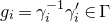 $g_i=\gamma_i^{-1}\gamma_i'\in \Gamma$
, we then have that
$g_i=\gamma_i^{-1}\gamma_i'\in \Gamma$
, we then have that ${\mu(g_i)}/{\|\mu(g_i)\|} \notin \mathcal C$
for all
${\mu(g_i)}/{\|\mu(g_i)\|} \notin \mathcal C$
for all $i \ge 1$
. Hence no limit of the sequence
$i \ge 1$
. Hence no limit of the sequence ${\mu(g_i)}/{\|\mu(g_i)\|} $
belongs to
${\mu(g_i)}/{\|\mu(g_i)\|} $
belongs to $\operatorname{{\rm int}} \mathcal C$
. On the other hand, since
$\operatorname{{\rm int}} \mathcal C$
. On the other hand, since $|g_i|\to \infty$
, we have
$|g_i|\to \infty$
, we have $\|\mu(g_i)\|\to \infty$
and hence any limit of the sequence
$\|\mu(g_i)\|\to \infty$
and hence any limit of the sequence ${\mu(g_i)}/{\|\mu(g_i)\|} $
must belong to the asymptotic cone of
${\mu(g_i)}/{\|\mu(g_i)\|} $
must belong to the asymptotic cone of $\mu(\Gamma)$
; that is,
$\mu(\Gamma)$
; that is, $\mathcal L$
. This yields a contradiction to the hypothesis
$\mathcal L$
. This yields a contradiction to the hypothesis $\mathcal L -\{0\} \subset \operatorname{{\rm int}}\mathcal C $
.
$\mathcal L -\{0\} \subset \operatorname{{\rm int}}\mathcal C $
.
The rest of this section is devoted to the proof of Theorem 4.3. We begin by recalling the following theorem; in particular, the metric space Z in Theorem 4.3 is always Gromov hyperbolic.
Theorem 4.5 [Reference Kapovich, Leeb and PortiKLP18, Theorem 1.4]. Let Z and $ f:Z\to X$
be as in Theorem 4.3. Then Z is Gromov hyperbolic. If Z is proper in addition, then f continuously extends to
$ f:Z\to X$
be as in Theorem 4.3. Then Z is Gromov hyperbolic. If Z is proper in addition, then f continuously extends to
 $$ f : \bar Z \to X \cup \mathcal F_{\theta},$$
where $\bar Z = Z \cup \partial Z$
is the Gromov compactification and f maps two distinct points in
$\bar Z = Z \cup \partial Z$
is the Gromov compactification and f maps two distinct points in $\partial Z$
to points in general position.
$\partial Z$
to points in general position.
4.3 Diamonds
The notion of diamonds in X, due to Kapovich, Leeb, and Porti, plays a key role in the proof of Theorem 4.3. We fix
 $$\text{a $\theta$-admissible cone $\mathcal C \subset \mathfrak a^+$ }$$
in the following. For a $\mathcal C$
-regular pair
$\mathcal C$
-regular pair $(x_1,x_2)$
of points in X, define the
$(x_1,x_2)$
of points in X, define the $\mathcal C$
-cone with the tip at
$\mathcal C$
-cone with the tip at $x_1$
containing
$x_1$
containing $x_2$
to be
$x_2$
to be
 \[ V_{\mathcal C}(x_1,x_2) = gM_{\theta}(\exp \mathcal C) o, \]
where $g=g(x_1, x_2) \in G$
is any element such that
$g=g(x_1, x_2) \in G$
is any element such that $x_1 = go$
and
$x_1 = go$
and $x_2 \in g (\exp \mathcal C) o$
; it is easy to check such g always exists and this definition is independent of the choice of g. For any
$x_2 \in g (\exp \mathcal C) o$
; it is easy to check such g always exists and this definition is independent of the choice of g. For any $h\in G$
, we have
$h\in G$
, we have $ hV_{\mathcal C}(x_1,x_2) = V_{\mathcal C}( hx_1, hx_2) $
.
$ hV_{\mathcal C}(x_1,x_2) = V_{\mathcal C}( hx_1, hx_2) $
.
Definition 4.6 (Diamonds) For a $\mathcal C$
-regular pair
$\mathcal C$
-regular pair $(x_1,x_2)$
of points in X, the
$(x_1,x_2)$
of points in X, the $\mathcal C$
-diamond with tips at
$\mathcal C$
-diamond with tips at $x_1$
and
$x_1$
and $x_2$
is defined as
$x_2$
is defined as
 \[ \Diamond_{\mathcal C}(x_1,x_2) = V_{\mathcal C}(x_1,x_2) \cap V_{\mathcal C}(x_2,x_1). \]
The $\mathcal C$
-cones and
$\mathcal C$
-cones and $\mathcal C$
-diamonds are convex subsets of X (see [Reference Kapovich, Leeb and PortiKLP17, Propositions 2.10 and 2.13]). Note also the equivariance property that for
$\mathcal C$
-diamonds are convex subsets of X (see [Reference Kapovich, Leeb and PortiKLP17, Propositions 2.10 and 2.13]). Note also the equivariance property that for $h\in G$
,
$h\in G$
, $ h \Diamond_{\mathcal C}(x_1,x_2) = \Diamond_{\mathcal C}(hx_1, hx_2) $
. It follows that for any
$ h \Diamond_{\mathcal C}(x_1,x_2) = \Diamond_{\mathcal C}(hx_1, hx_2) $
. It follows that for any $\mathcal C$
-regular pair
$\mathcal C$
-regular pair $(x_1, x_2)$
, the diamond
$(x_1, x_2)$
, the diamond $\Diamond_{\mathcal C}(x_1,x_2)$
is of the form
$\Diamond_{\mathcal C}(x_1,x_2)$
is of the form $h \Diamond_{\mathcal C}(o,ao)$
for some
$h \Diamond_{\mathcal C}(o,ao)$
for some $a\in \exp \mathcal C$
and
$a\in \exp \mathcal C$
and $h\in G$
. Therefore, the following example describes all diamonds up to translations.
$h\in G$
. Therefore, the following example describes all diamonds up to translations.
Example 4.7. For $a \in \exp \mathcal C$
, the diamond
$a \in \exp \mathcal C$
, the diamond $\Diamond_{\mathcal C}(o, a o)$
can be explicitly described as follows. First note that as we can take
$\Diamond_{\mathcal C}(o, a o)$
can be explicitly described as follows. First note that as we can take $g(o, ao) =e$
, we have
$g(o, ao) =e$
, we have $V_{\mathcal C}(o, a o) = M_{\theta}(\exp \mathcal C) o.$
Recalling that
$V_{\mathcal C}(o, a o) = M_{\theta}(\exp \mathcal C) o.$
Recalling that ${\rm i}=-\operatorname{{\rm Ad}}_{w_0}$
, we also have
${\rm i}=-\operatorname{{\rm Ad}}_{w_0}$
, we also have $a o = a w_0 o $
and
$a o = a w_0 o $
and $ o = (aw_0) (w_0^{-1} a^{-1} w_0) o \in aw_0 (\exp \mathcal C) o .$
So we can take
$ o = (aw_0) (w_0^{-1} a^{-1} w_0) o \in aw_0 (\exp \mathcal C) o .$
So we can take $g(ao, o)=aw_0$
. Since
$g(ao, o)=aw_0$
. Since $w_0 M_{\theta} w_0^{-1} = M_{\theta}$
and
$w_0 M_{\theta} w_0^{-1} = M_{\theta}$
and $w_0 (\exp \mathcal C) w_0^{-1} = \exp (-\mathcal C)$
, we have
$w_0 (\exp \mathcal C) w_0^{-1} = \exp (-\mathcal C)$
, we have $V_{\mathcal C}(a o, o) = a w_0 M_{\theta} (\exp \mathcal C) o = a M_{\theta} \exp (- \mathcal C) o$
. Therefore,
$V_{\mathcal C}(a o, o) = a w_0 M_{\theta} (\exp \mathcal C) o = a M_{\theta} \exp (- \mathcal C) o$
. Therefore,
 $$ \Diamond_{\mathcal C}(o, a o) = M_{\theta} (\exp \mathcal C) o \cap a M_{\theta} \exp(-\mathcal C) o$$
(see Figure 4.7).
A diamond drawn in $\mathfrak a$
.
$\mathfrak a$
.

Lemma 4.8 (Simultaneous nesting property) If $(x_1, x_2)$
is
$(x_1, x_2)$
is $\mathcal C$
-regular, then for any
$\mathcal C$
-regular, then for any $x \in \Diamond_{\mathcal C}(x_1, x_2)$
, there exist
$x \in \Diamond_{\mathcal C}(x_1, x_2)$
, there exist $g \in G$
and
$g \in G$
and $a \in \exp \mathcal C$
such that
$a \in \exp \mathcal C$
such that
 $$x_1 = go, \quad x = ga o ,\quad x_2 \in g M_{\theta} (\exp \mathcal C) o \cap g a (M_{\theta} \exp \mathcal C) o.$$
Proof. We may first assume that $x_1 = o$
. By the
$x_1 = o$
. By the $\mathcal C$
-regularity of the pair
$\mathcal C$
-regularity of the pair $(x_1, x_2)$
, we have
$(x_1, x_2)$
, we have $x_2 \in K (\exp \mathcal C) o$
. By multiplying an element of K to
$x_2 \in K (\exp \mathcal C) o$
. By multiplying an element of K to $x_1$
and
$x_1$
and $x_2$
, we may also assume that
$x_2$
, we may also assume that $x_1 = o$
and
$x_1 = o$
and $x_2 \in (\exp \mathcal C) o$
, and hence
$x_2 \in (\exp \mathcal C) o$
, and hence $x \in M_{\theta} (\exp \mathcal C) o$
. We again multiply an element of
$x \in M_{\theta} (\exp \mathcal C) o$
. We again multiply an element of $M_{\theta}$
to
$M_{\theta}$
to $x_1, x_2$
, and x if necessary so that we have
$x_1, x_2$
, and x if necessary so that we have $x_1 = o$
,
$x_1 = o$
, $x_2 \in M_{\theta}(\exp \mathcal C) o$
, and
$x_2 \in M_{\theta}(\exp \mathcal C) o$
, and $x = ao$
for some
$x = ao$
for some $a \in \exp \mathcal C$
. Then it suffices to show that
$a \in \exp \mathcal C$
. Then it suffices to show that $x_2 = a k a' o$
for some
$x_2 = a k a' o$
for some $k \in M_{\theta}$
and
$k \in M_{\theta}$
and $a' \in \exp \mathcal C$
. We write
$a' \in \exp \mathcal C$
. We write $x_2 = m a_0 o$
for
$x_2 = m a_0 o$
for $m \in M_{\theta}$
and
$m \in M_{\theta}$
and $a_0 \in \exp \mathcal C$
. We then have
$a_0 \in \exp \mathcal C$
. We then have $ o \in V_{\mathcal C}(x_2, o) = m a_0 k_0 M_{\theta} (\exp \mathcal C) o$
for some
$ o \in V_{\mathcal C}(x_2, o) = m a_0 k_0 M_{\theta} (\exp \mathcal C) o$
for some $k_0 \in K$
. Hence, we have
$k_0 \in K$
. Hence, we have
 $$ k_0^{-1} w_0^{-1} (w_0 a_0^{-1} w_0^{-1}) \in M_{\theta} (\exp \mathcal C) K. $$
This implies that $k_0^{-1} \in M_{\theta} w_0$
and hence
$k_0^{-1} \in M_{\theta} w_0$
and hence $k_0 \in w_0 M_{\theta}$
. Since
$k_0 \in w_0 M_{\theta}$
. Since $a o \in V_{\mathcal C}(x_2, o)$
as well, we now have
$a o \in V_{\mathcal C}(x_2, o)$
as well, we now have $a o \in m a_0 w_0 M_{\theta} (\exp \mathcal C) o$
. Then, for some
$a o \in m a_0 w_0 M_{\theta} (\exp \mathcal C) o$
. Then, for some $k \in K$
, we have
$k \in K$
, we have
 $$ a k \in m a_0 w_0 M_{\theta} \exp \mathcal C w_0^{-1} = m a_0 M_{\theta} \exp (- \mathcal C). $$
Hence, for some $a' \in \exp \mathcal C$
, we have
$a' \in \exp \mathcal C$
, we have
 $$a k a' \in m a_0 M_{\theta}.$$
Looking at $G/P_{\theta}$
, we have
$G/P_{\theta}$
, we have $ k P_{\theta} = a^{-1} m a_0 M_{\theta} a'^{-1} P_{\theta} = P_{\theta}$
. Therefore,
$ k P_{\theta} = a^{-1} m a_0 M_{\theta} a'^{-1} P_{\theta} = P_{\theta}$
. Therefore, $k \in M_{\theta}$
. Since
$k \in M_{\theta}$
. Since $x_2 = m a_0 o = aka' o$
, the claim follows.
$x_2 = m a_0 o = aka' o$
, the claim follows.
Lemma 4.9.
For any $\mathcal C$
-regular pair
$\mathcal C$
-regular pair $(g_1 o, g_2 o)$
with
$(g_1 o, g_2 o)$
with $g_1, g_2\in G$
and for any
$g_1, g_2\in G$
and for any $ go \in \Diamond_{\mathcal C}(g_1 o, g_2 o)$
with
$ go \in \Diamond_{\mathcal C}(g_1 o, g_2 o)$
with $g\in G$
,
$g\in G$
,
 \begin{equation} \mu_{\theta}(g_1^{-1}g) + \mu_{\theta}(g^{-1} g_2) = \mu_{\theta}(g_1^{-1}g_2).\end{equation}
Proof. By Lemma 4.8, there exists $h\in G$
,
$h\in G$
, $a, \tilde{a}, a' \in \exp \mathcal C$
and
$a, \tilde{a}, a' \in \exp \mathcal C$
and $\tilde{k}, k \in M_\theta $
such that
$\tilde{k}, k \in M_\theta $
such that $g_1o=ho$
,
$g_1o=ho$
, $go=hao$
, and
$go=hao$
, and $g_2o= h \tilde{k} \tilde{a} o = ha k a'o$
. Without loss of generality, we may assume that
$g_2o= h \tilde{k} \tilde{a} o = ha k a'o$
. Without loss of generality, we may assume that $h=e$
in proving (4.2).
$h=e$
in proving (4.2).
We write
 $$ a = a_1 a_2 \in A_{\theta}^+B_{\theta}^+ \quad \text{and }\quad a' = a_1' a_2' \in A_{\theta}^+ B_{\theta}^+. $$
We then have
 $$aka' = a_2 k a_2' (a_1a_1').$$
Since $a_2 k a_2' \in S_{\theta}$
, we can write its Cartan decomposition
$a_2 k a_2' \in S_{\theta}$
, we can write its Cartan decomposition $a_2 k a_2' = m b m' \in M_{\theta}B_{\theta}^+M_{\theta}$
, and hence
$a_2 k a_2' = m b m' \in M_{\theta}B_{\theta}^+M_{\theta}$
, and hence
 $$aka' = m (b a_1 a_1')m'.$$
Let $w \in \mathcal W$
be a Weyl element such that
$w \in \mathcal W$
be a Weyl element such that $b a_1 a_1' \in w A^+ w^{-1}$
. Since
$b a_1 a_1' \in w A^+ w^{-1}$
. Since $\tilde{a} = \exp \mu(aka')$
, we must have
$\tilde{a} = \exp \mu(aka')$
, we must have $b a_1 a_1' = w \tilde{a} w^{-1}$
. Hence we have
$b a_1 a_1' = w \tilde{a} w^{-1}$
. Hence we have
 $$g_2 o = aka' o = m w \tilde{a} o.$$
On the other hand, we also have $g_2 o = \tilde{k} \tilde{a} o,$
where
$g_2 o = \tilde{k} \tilde{a} o,$
where $\tilde{k} \in M_{\theta}$
. This implies that
$\tilde{k} \in M_{\theta}$
. This implies that $mw \in M_{\theta}$
; and, in particular,
$mw \in M_{\theta}$
; and, in particular, $w \in M_{\theta}$
. Therefore
$w \in M_{\theta}$
. Therefore $\tilde{a} = w^{-1} b a_1 a_1' w = (w^{-1} b w)(a_1 a_1') \in B_{\theta}A_{\theta}^+$
, which implies that
$\tilde{a} = w^{-1} b a_1 a_1' w = (w^{-1} b w)(a_1 a_1') \in B_{\theta}A_{\theta}^+$
, which implies that
 \begin{equation} p_{\theta}(\log \tilde{a}) = \log a_1 + \log a_1' = p_{\theta}(\log a) + p_{\theta}(\log a').\end{equation}
Since
 $$ \mu_{\theta}(g_1^{-1} g) = p_{\theta}(\log a), \quad \mu_{\theta}(g^{-1} g_2) = p_{\theta}(\log a'),\quad \text{and} \quad \mu_{\theta}(g_1^{-1}g_2) = p_{\theta}(\log \tilde{a}),$$
this finishes the proof.
As an immediate corollary, we obtain that $\mathsf{d}_{\psi}$
is additive on each diamond for any
$\mathsf{d}_{\psi}$
is additive on each diamond for any $\psi\in \mathfrak a_\theta^*$
.
$\psi\in \mathfrak a_\theta^*$
.
Lemma 4.10 (Additivity of $\mathsf{d}_\psi$
on diamonds) Let
$\mathsf{d}_\psi$
on diamonds) Let $\psi \in \mathfrak a_{\theta}^*$
. For any
$\psi \in \mathfrak a_{\theta}^*$
. For any $\mathcal C$
-regular pair
$\mathcal C$
-regular pair $(x_1, x_2)$
and for any
$(x_1, x_2)$
and for any $x\in \Diamond_{\mathcal C}(x_1, x_2)$
, we have
$x\in \Diamond_{\mathcal C}(x_1, x_2)$
, we have
 $$\mathsf{d}_\psi(x_1,x)+ \mathsf{d}_{\psi}(x,x_2) = \mathsf{d}_\psi(x_1,x_2).$$
4.4 KLP Morse lemma
The Morse lemma due to Kapovich, Leeb, and Porti, which we will call the KLP Morse lemma, is stated as follows [Reference Kapovich, Leeb and PortiKLP18, Theorem 5.16, Corollary 5.28]: the image of an interval in $\mathbb R $
under a Q-quasi-isometry is called a Q-quasi-geodesic.
$\mathbb R $
under a Q-quasi-isometry is called a Q-quasi-geodesic.
Theorem 4.11 (KLP Morse lemma) Let $\mathcal C,\mathcal C' \subset \mathfrak a^+$
be
$\mathcal C,\mathcal C' \subset \mathfrak a^+$
be $\theta$
-admissible closed cones such that
$\theta$
-admissible closed cones such that $\operatorname{{\rm int}} \mathcal C'$
contains
$\operatorname{{\rm int}} \mathcal C'$
contains $ \mathcal C-\{0\}$
(see Figure 2). Let
$ \mathcal C-\{0\}$
(see Figure 2). Let $Q, B\ge 1$
be constants. There exists a constant
$Q, B\ge 1$
be constants. There exists a constant $D_0 = D_0(\mathcal C,\mathcal C', Q, B) \ge 0$
so that the following holds: let
$D_0 = D_0(\mathcal C,\mathcal C', Q, B) \ge 0$
so that the following holds: let $I \subset \mathbb R$
be an interval and
$I \subset \mathbb R$
be an interval and $c : I \to X$
a
$c : I \to X$
a $(\mathcal C, B)$
-regular Q-quasi-geodesic.
$(\mathcal C, B)$
-regular Q-quasi-geodesic.
The choice of $\mathcal C'$
viewed on the unit sphere of
$\mathcal C'$
viewed on the unit sphere of $\mathfrak a^+$
.
$\mathfrak a^+$
.

-
(1) If
$I = [a, b]$
with
$b - a \ge B$
, then the image c(I) is contained in the
$D_0$
-neighborhood of the diamond
$\Diamond_{\mathcal C'}(c(a),c(b))$
. -
(2) If
$I = [a, \infty)$
for some
$a \in \mathbb R$
, then c(I) is contained in the
$D_0$
-neighborhood of the cone
$g M_{\theta}(\exp \mathcal C') o,$
where
$g \in G$
is such that
$g o = c(a)$
and
$g^+ = c(\infty) \in \mathcal F_{\theta}$
. -
(3) If
$I = \mathbb R$
, then c(I) is contained in the
$D_0$
-neighborhood of the parallel set
$g M_{\theta} A o,$
where
$g \in G$
is such that
$g^{\pm} = c(\pm \infty) \in \mathcal F_{\theta}$
.












We note that the above applies for an interval in $\mathbb Z$
, as any
$\mathbb Z$
, as any $\mathcal C$
-regular quasi-isometric embedding
$\mathcal C$
-regular quasi-isometric embedding $c:I\cap \mathbb Z \to X$
can be extended to a
$c:I\cap \mathbb Z \to X$
can be extended to a $\mathcal C$
-regular quasi-geodesic
$\mathcal C$
-regular quasi-geodesic $I\to X$
simply by setting
$I\to X$
simply by setting $c(t) := c( \lfloor t \rfloor)$
where
$c(t) := c( \lfloor t \rfloor)$
where $\lfloor t \rfloor$
is the largest integer not bigger than t.
$\lfloor t \rfloor$
is the largest integer not bigger than t.
As an application of Theorem 4.11, we obtain the following.
Corollary 4.12
Given $\mathcal C, \mathcal C', Q, B\ge 1$
as in Theorem 4.11 and
$\mathcal C, \mathcal C', Q, B\ge 1$
as in Theorem 4.11 and $\psi\in \mathfrak a_\theta^*$
, there exists a constant
$\psi\in \mathfrak a_\theta^*$
, there exists a constant $D_1 = D_1(\mathcal C,\mathcal C', Q, B,\psi) \ge 0$
so that the following holds: let
$D_1 = D_1(\mathcal C,\mathcal C', Q, B,\psi) \ge 0$
so that the following holds: let $I \subset \mathbb R$
be an interval and
$I \subset \mathbb R$
be an interval and $c : I \to X$
a
$c : I \to X$
a $(\mathcal C, B)$
-regular Q-quasi-geodesic. Then, for all
$(\mathcal C, B)$
-regular Q-quasi-geodesic. Then, for all $a \le t \le b$
in I, we have
$a \le t \le b$
in I, we have
 \begin{equation} |\mathsf{d}_\psi( c(a), c(b)) - \mathsf{d}_\psi( c(a), c(t)) - \mathsf{d}_\psi(c(t), c(b))| \le D_1. \end{equation}
Proof. Suppose that $b - a \ge B$
. Since c is
$b - a \ge B$
. Since c is $(\mathcal C, B)$
-regular, the pair (c(a), c(b)) is
$(\mathcal C, B)$
-regular, the pair (c(a), c(b)) is $\mathcal C$
-regular. Applying Theorem 4.11, we obtain that the image of
$\mathcal C$
-regular. Applying Theorem 4.11, we obtain that the image of $ c : [a,b] \to X$
lies in the
$ c : [a,b] \to X$
lies in the $D_0$
-neighborhood of
$D_0$
-neighborhood of $\Diamond_{\mathcal C'}(c(a), c(b))$
. For each
$\Diamond_{\mathcal C'}(c(a), c(b))$
. For each $a \lt t \lt b$
, choose
$a \lt t \lt b$
, choose $x_t\in \Diamond_{\mathcal C'}(c(a), c(b))$
so that
$x_t\in \Diamond_{\mathcal C'}(c(a), c(b))$
so that $d(x_t, c(t)) \le D_0$
. Hence, by Lemma 4.10,
$d(x_t, c(t)) \le D_0$
. Hence, by Lemma 4.10,
 \begin{equation} \mathsf{d}_\psi(c(a),x_t)+ \mathsf{d}_{\psi}(x_t, c(b)) = \mathsf{d}_\psi(c(a),c(b)). \end{equation}
For each $a \le t \le b$
, write
$a \le t \le b$
, write $c(t)=g_t o$
and
$c(t)=g_t o$
and $x_t=h_t o$
for
$x_t=h_t o$
for $g_t, h_t\in G$
. We then have
$g_t, h_t\in G$
. We then have $\| \mu(h_t^{-1} g_t)\|\le D_0$
. By applying Lemma 2.1 to a compact subset
$\| \mu(h_t^{-1} g_t)\|\le D_0$
. By applying Lemma 2.1 to a compact subset $\{g \in G : \|\mu(g)\|\le D_0\}$
, we have, for all
$\{g \in G : \|\mu(g)\|\le D_0\}$
, we have, for all $a\lt t\lt b$
,
$a\lt t\lt b$
,
 $$|\mathsf{d}_{\psi}(c(a), x_t) - \mathsf{d}_{\psi}(c(a) , c(t)) | = | \psi( \mu(g_a^{-1} h_t) - \mu(g_a^{-1} g_t )) | \le C,$$
where $C\gt 0$
is a uniform constant depending only on
$C\gt 0$
is a uniform constant depending only on $\psi$
and
$\psi$
and $D_0$
. Similarly, we have
$D_0$
. Similarly, we have $|\mathsf{d}_\psi (x_t, c(b)) - \mathsf{d}_\psi (c(t), c(b)) |\le C $
. By (4.5), this implies that
$|\mathsf{d}_\psi (x_t, c(b)) - \mathsf{d}_\psi (c(t), c(b)) |\le C $
. By (4.5), this implies that
 $$ |\mathsf{d}_\psi( c(a), c(b)) - \mathsf{d}_\psi( c(a), c(t)) - \mathsf{d}_\psi(c(t), c(b))| \le 2 C. $$
Setting $D_1= 2C + 3 \|\psi\|(QB + Q)$
, where
$D_1= 2C + 3 \|\psi\|(QB + Q)$
, where $\|\psi\|$
is the operator norm of
$\|\psi\|$
is the operator norm of $\psi$
, we have shown that (4.4) holds whenever
$\psi$
, we have shown that (4.4) holds whenever $b-a\ge B$
. If
$b-a\ge B$
. If $b - a \lt B$
, then the image of c([a, b]) has diameter smaller than
$b - a \lt B$
, then the image of c([a, b]) has diameter smaller than $Q(b-a) + Q \lt QB + Q$
. Then,
$Q(b-a) + Q \lt QB + Q$
. Then,
 $$\mathsf{d}_{\psi}(c(t_1), c(t_2)) \lt \|\psi\| (QB + Q)$$
for all $t_1, t_2 \in [a, b]$
, and hence the left-hand side of (4.4) is bounded above by
$t_1, t_2 \in [a, b]$
, and hence the left-hand side of (4.4) is bounded above by $ 3\|\psi\| (QB + Q)\le D_1$
. This completes the proof.
$ 3\|\psi\| (QB + Q)\le D_1$
. This completes the proof.
We are ready to give the following proof.
4.5 Proof of Theorem 4.3
Let $f : Z \to X$
be as in Theorem 4.3. Let
$f : Z \to X$
be as in Theorem 4.3. Let $\psi \in \mathfrak a_{\theta}^*$
be such that
$\psi \in \mathfrak a_{\theta}^*$
be such that $\psi \gt 0$
on
$\psi \gt 0$
on $ \mathcal C - \{0\}$
. Choose a
$ \mathcal C - \{0\}$
. Choose a $\theta$
-admissible cone
$\theta$
-admissible cone $\mathcal C' \subset \mathfrak a^+$
such that
$\mathcal C' \subset \mathfrak a^+$
such that $\operatorname{{\rm int}} \mathcal C'$
contains
$\operatorname{{\rm int}} \mathcal C'$
contains $\mathcal C-\{0\}$
and such that
$\mathcal C-\{0\}$
and such that $\psi\gt 0$
on
$\psi\gt 0$
on $\mathcal C'-\{0\}$
. Let
$\mathcal C'-\{0\}$
. Let $x_1, x_2, x_3 \in f(Z)$
be a triple of distinct points. We choose
$x_1, x_2, x_3 \in f(Z)$
be a triple of distinct points. We choose $z_1, z_2, z_3 \in Z$
such that
$z_1, z_2, z_3 \in Z$
such that $x_i = f(z_i)$
for
$x_i = f(z_i)$
for $i = 1,2, 3$
. Choose geodesics
$i = 1,2, 3$
. Choose geodesics $c_1$
and
$c_1$
and $c_2$
in Z connecting
$c_2$
in Z connecting $z_1$
to
$z_1$
to $z_2$
and
$z_2$
and $z_2$
to
$z_2$
to $z_3$
, respectively. By Theorem 4.5,
$z_3$
, respectively. By Theorem 4.5, $(Z, d_Z)$
is Gromov hyperbolic. We denote by z the nearest-point projection of
$(Z, d_Z)$
is Gromov hyperbolic. We denote by z the nearest-point projection of $z_2$
to a geodesic segment connecting
$z_2$
to a geodesic segment connecting $z_1$
and
$z_1$
and $z_3$
. Then, by the Gromov hyperbolicity of
$z_3$
. Then, by the Gromov hyperbolicity of $(Z, d_Z)$
, there exists a uniform constant
$(Z, d_Z)$
, there exists a uniform constant $\delta \gt 0$
so that the
$\delta \gt 0$
so that the $\delta$
-neighborhood of z intersects both geodesics
$\delta$
-neighborhood of z intersects both geodesics $c_1$
and
$c_1$
and $c_2$
. We choose two points
$c_2$
. We choose two points $y_1 \in c_1$
and
$y_1 \in c_1$
and $y_2 \in c_2$
that are
$y_2 \in c_2$
that are $\delta$
-close to z. We concatenate the segment of
$\delta$
-close to z. We concatenate the segment of $c_1$
connecting
$c_1$
connecting $z_1$
and
$z_1$
and $y_1$
, a geodesic connecting
$y_1$
, a geodesic connecting $y_1$
and
$y_1$
and $y_2$
, and the segment of
$y_2$
, and the segment of $c_2$
connecting
$c_2$
connecting $y_2$
and
$y_2$
and $z_3$
, and denote the concatenated path by c. We can parameterize
$z_3$
, and denote the concatenated path by c. We can parameterize $c : [0, b] \to Z$
so that c is a q-quasi-geodesic for some
$c : [0, b] \to Z$
so that c is a q-quasi-geodesic for some $b \gt 0$
and uniform
$b \gt 0$
and uniform $q \ge 1$
by the Gromov hyperbolicity of
$q \ge 1$
by the Gromov hyperbolicity of $(Z, d_Z)$
and the choice of
$(Z, d_Z)$
and the choice of $y_1$
and
$y_1$
and $y_2$
.
$y_2$
.
Since f is a $\mathcal C$
-regular quasi-isometric embedding, so is
$\mathcal C$
-regular quasi-isometric embedding, so is $f \circ c$
. Hence, we obtain
$f \circ c$
. Hence, we obtain
 \begin{equation} \mathsf{d}_\psi(x_1, x_3) \le \mathsf{d}_\psi(x_1, f(y_1)) + \mathsf{d}_\psi( f(y_1) ,x_3) +D_1,\end{equation}
where $D_1$
is the constant given by Corollary 4.12. Applying Corollary 4.12 to the restriction of
$D_1$
is the constant given by Corollary 4.12. Applying Corollary 4.12 to the restriction of $f \circ c$
to the interval
$f \circ c$
to the interval $[c^{-1}(y_1), b]$
again, we have
$[c^{-1}(y_1), b]$
again, we have
 \begin{equation} \mathsf{d}_\psi( f(y_1) ,x_3) \le \mathsf{d}_\psi(f(y_1), f(y_2)) + \mathsf{d}_{\psi}( f(y_2), x_3) + D_1.\end{equation}
Since $d_Z(y_1, y_2) \le 2 \delta$
, combining (4.6) and (4.7) yields
$d_Z(y_1, y_2) \le 2 \delta$
, combining (4.6) and (4.7) yields
 \begin{equation} \mathsf{d}_{\psi}(x_1, x_3) \le \mathsf{d}_\psi(x_1, f(y_1)) + \mathsf{d}_{\psi}( f(y_2), x_3) + D_1',\end{equation}
where $D_1':= \sup \{\mathsf{d}_\psi(f(w_1), f(w_2)) :{d_Z(w_1, w_2) \le 2 \delta} \} + 2 D_1\lt \infty $
.
$D_1':= \sup \{\mathsf{d}_\psi(f(w_1), f(w_2)) :{d_Z(w_1, w_2) \le 2 \delta} \} + 2 D_1\lt \infty $
.
Since f is $\mathcal C$
-regular and
$\mathcal C$
-regular and $\psi \gt 0$
on
$\psi \gt 0$
on $\mathcal C - \{0\}$
, there exists
$\mathcal C - \{0\}$
, there exists $D_2 \gt 0$
such that
$D_2 \gt 0$
such that
 \begin{equation} \mathsf{d}_{\psi}(f(w_1), f(w_2)) \ge - D_2\end{equation}
for all $w_1, w_2 \in Z$
; indeed, if f is
$w_1, w_2 \in Z$
; indeed, if f is $(\mathcal C, B)$
-regular for some
$(\mathcal C, B)$
-regular for some $B\ge0$
, then
$B\ge0$
, then $\mathsf{d}_{\psi}(f(w_1), f(w_2)) \ge 0$
whenever
$\mathsf{d}_{\psi}(f(w_1), f(w_2)) \ge 0$
whenever $d_Z(w_1, w_2)\ge B$
, and
$d_Z(w_1, w_2)\ge B$
, and $\sup \{|\mathsf{d}_\psi (f(w_1), f(w_2))| :d_Z(w_1, w_2)\lt B\} $
is bounded by a uniform constant depending only on B, the quasi-isometry constant of f, and
$\sup \{|\mathsf{d}_\psi (f(w_1), f(w_2))| :d_Z(w_1, w_2)\lt B\} $
is bounded by a uniform constant depending only on B, the quasi-isometry constant of f, and $\|\psi\|$
.
$\|\psi\|$
.
Hence, applying (4.9) and Corollary 4.12 to $f ( c_1 )$
, we have
$f ( c_1 )$
, we have
 \begin{align} \mathsf{d}_\psi (x_1, f(y_1)) & \le \mathsf{d}_\psi (x_1, f(y_1)) +\mathsf{d}_\psi(f(y_1),x_2) + D_2\nonumber\\ & \le \mathsf{d}_\psi(x_1,x_2) +D_1 + D_2.\end{align}
Similarly, we also obtain
 \begin{equation} \mathsf{d}_\psi(f(y_2),x_3) \le \mathsf{d}_\psi(x_2,x_3)+D_1 + D_2. \end{equation}
Combining (4.8), (4.10), and (4.11), we obtain
 $$ \mathsf{d}_{\psi}(x_1, x_3) \le \mathsf{d}_{\psi}(x_1, x_2) + \mathsf{d}_{\psi}(x_2, x_3) + D_1' + 2( D_1 + D_2). $$
This completes the proof of Theorem 4.3.
We state the following consequence of the KLP Morse lemma applied to Anosov subgroups.
Theorem 4.13 (Morse lemma for Anosov subgroups) Let $\theta={\rm i}(\theta)$
. Let
$\theta={\rm i}(\theta)$
. Let $\Gamma$
be a
$\Gamma$
be a $\theta$
-Anosov subgroup and let
$\theta$
-Anosov subgroup and let $f : \Gamma \cup \partial \Gamma \to \Gamma o \cup \Lambda_{\theta}$
be the extension of the orbit map
$f : \Gamma \cup \partial \Gamma \to \Gamma o \cup \Lambda_{\theta}$
be the extension of the orbit map $\gamma \mapsto \gamma o$
given in Theorem 3.8(4). Then there exist a cone
$\gamma \mapsto \gamma o$
given in Theorem 3.8(4). Then there exist a cone $\mathcal C \subset \mathfrak a^+$
and constants
$\mathcal C \subset \mathfrak a^+$
and constants $B, D_0 \ge 1$
such that for any geodesic
$B, D_0 \ge 1$
such that for any geodesic $[\xi, \eta]$
in
$[\xi, \eta]$
in $\Gamma$
, the following hold.
$\Gamma$
, the following hold.
-
(1) If
$\xi, \eta \in \Gamma$
and
$\mathsf{d}_{\Gamma}(\xi, \eta) \ge B$
, then
$f([\xi, \eta])$
is contained in the
$D_0$
-neighborhood of the diamond
$\Diamond_{\mathcal C}(f(\xi), f(\eta))$
. -
(2) If
$\xi \in \Gamma$
and
$\eta \in \partial \Gamma$
, then
$f([\xi, \eta])$
is contained in the
$D_0$
-neighborhood of
$g M_{\theta} (\exp \mathcal C) o$
, where
$g \in G$
is such that
$g o = \xi$
and
$g P_{\theta} = f(\eta)$
. -
(3) If
$\xi, \eta \in \partial \Gamma$
, then
$f([\xi, \eta])$
is contained in the
$D_0$
-neighborhood of
$g M_{\theta} A o$
, where
$g \in G$
is such that
$g P_{\theta} = f(\xi)$
and
$g w_0 P_{\theta} = f(\eta)$
.






Moreover, the cone $\mathcal C$
can be taken arbitrarily close to
$\mathcal C$
can be taken arbitrarily close to $\mathcal L$
as long as its interior contains
$\mathcal L$
as long as its interior contains $\mathcal L - \{0\}$
.
$\mathcal L - \{0\}$
.
Proof. Let $\mathcal C\subset \mathfrak a^+$
be the
$\mathcal C\subset \mathfrak a^+$
be the $\theta$
-admissible cone as in the proof of Theorem 4.1, and choose a
$\theta$
-admissible cone as in the proof of Theorem 4.1, and choose a $\theta$
-admissible cone
$\theta$
-admissible cone $\mathcal C' \subset \mathfrak a^+$
whose interior in
$\mathcal C' \subset \mathfrak a^+$
whose interior in $\mathfrak a^+$
contains
$\mathfrak a^+$
contains $\mathcal C-\{0\}$
. Then, by Lemma 4.4 and Theorem 3.8(3), the orbit map
$\mathcal C-\{0\}$
. Then, by Lemma 4.4 and Theorem 3.8(3), the orbit map $f|_{\Gamma}$
is a
$f|_{\Gamma}$
is a $(\mathcal C, B) $
-regular Q-quasi-isometry between
$(\mathcal C, B) $
-regular Q-quasi-isometry between $(\Gamma, \mathsf{d}_\Gamma)$
and
$(\Gamma, \mathsf{d}_\Gamma)$
and $(\Gamma o, d)$
for some
$(\Gamma o, d)$
for some $B, Q\ge 1$
. Let
$B, Q\ge 1$
. Let $D_0=D_0(\mathcal C, \mathcal C', Q, B)$
be as given by Theorem 4.11.
$D_0=D_0(\mathcal C, \mathcal C', Q, B)$
be as given by Theorem 4.11.
Now note that any geodesic $[\xi,\eta]$
in
$[\xi,\eta]$
in $(\Gamma, \mathsf{d}_\Gamma)$
can be written as
$(\Gamma, \mathsf{d}_\Gamma)$
can be written as $[\xi, \eta]=\{\gamma_i:i\in I\}$
for an interval I in
$[\xi, \eta]=\{\gamma_i:i\in I\}$
for an interval I in $\mathbb Z$
, and
$\mathbb Z$
, and $\iota: i\mapsto \gamma_i$
is an isometry between I and
$\iota: i\mapsto \gamma_i$
is an isometry between I and $[\xi, \eta]$
. Since
$[\xi, \eta]$
. Since $c:=f \circ \iota $
is a
$c:=f \circ \iota $
is a $(\mathcal C, B)$
-regular Q-quasi-geodesic, we can apply Theorem 4.11, which implies the above claims (1)–(3), where the cone
$(\mathcal C, B)$
-regular Q-quasi-geodesic, we can apply Theorem 4.11, which implies the above claims (1)–(3), where the cone $\mathcal C$
in the statement is given by
$\mathcal C$
in the statement is given by $\mathcal C'$
in this proof. Note from the proof of Theorem 4.1 that the cone
$\mathcal C'$
in this proof. Note from the proof of Theorem 4.1 that the cone $\mathcal C'$
can be taken arbitrarily close to the limit cone
$\mathcal C'$
can be taken arbitrarily close to the limit cone $\mathcal L$
of
$\mathcal L$
of $\Gamma$
as long as
$\Gamma$
as long as $\operatorname{{\rm int}} \mathcal C'$
contains
$\operatorname{{\rm int}} \mathcal C'$
contains $\mathcal L - \{0\}$
.
$\mathcal L - \{0\}$
.
5. Conformal premetrics on limit sets
Let $\Gamma$
be a
$\Gamma$
be a $\theta$
-Anosov subgroup of a connected semisimple real algebraic group G. We assume that
$\theta$
-Anosov subgroup of a connected semisimple real algebraic group G. We assume that $\theta = {\rm i}(\theta)$
in this section. Fix a linear form
$\theta = {\rm i}(\theta)$
in this section. Fix a linear form $\psi \in \mathfrak a_\theta^*$
positive on
$\psi \in \mathfrak a_\theta^*$
positive on $\mathcal L_{\theta} - \{0\}$
. The goal of this section is to define a premetric
$\mathcal L_{\theta} - \{0\}$
. The goal of this section is to define a premetric $d_\psi$
on the limit set
$d_\psi$
on the limit set $\Lambda_\theta$
, which is conformal, almost symmetric and satisfies almost triangle inequality with bounded multiplicative error. We also discuss how this definition can be extended to non-symmetric
$\Lambda_\theta$
, which is conformal, almost symmetric and satisfies almost triangle inequality with bounded multiplicative error. We also discuss how this definition can be extended to non-symmetric $\theta$
at the end of the section.
$\theta$
at the end of the section.
Recall the definition of the Gromov product from Definition 2.3. The $\theta$
-Anosov property of
$\theta$
-Anosov property of $\Gamma$
implies that any two distinct points in
$\Gamma$
implies that any two distinct points in $\Lambda_\theta$
are in general position: if
$\Lambda_\theta$
are in general position: if $\xi\ne \eta$
in
$\xi\ne \eta$
in $\Lambda_\theta$
, then
$\Lambda_\theta$
, then $(\xi, \eta)\in \mathcal F_\theta^{(2)}$
. Therefore, the following premetric on
$(\xi, \eta)\in \mathcal F_\theta^{(2)}$
. Therefore, the following premetric on $\Lambda_\theta$
is well-defined.
$\Lambda_\theta$
is well-defined.
Definition 5.1.
For $\xi, \eta \in \Lambda_{\theta}$
, we set
$\xi, \eta \in \Lambda_{\theta}$
, we set
 \begin{equation}d_{\psi}(\xi, \eta) =\begin{cases}e^{-\psi( \mathcal G^{\theta}(\xi, \eta))} & \text{if } \xi \neq \eta,\\0 &\text {if } \xi = \eta.\end{cases} \end{equation}
We first observe the following $\Gamma$
-conformal property of
$\Gamma$
-conformal property of $d_\psi$
.
$d_\psi$
.
Lemma 5.2.
For $\gamma \in \Gamma$
and
$\gamma \in \Gamma$
and $\xi, \eta \in \Lambda_{\theta}$
, we have
$\xi, \eta \in \Lambda_{\theta}$
, we have
 $$ d_{\psi}(\gamma^{-1}\xi, \gamma^{-1}\eta) = e^{(1/2)\psi(\beta_{\xi}^{\theta}(e, \gamma) + {\rm i} (\beta_{\eta}^{\theta}(e, \gamma )))} d_{\psi}(\xi, \eta). $$
Proof. Let $\xi \neq \eta$
, and
$\xi \neq \eta$
, and $g \in G$
be such that
$g \in G$
be such that $g^+ = \xi$
and
$g^+ = \xi$
and $g^- = \eta$
. Then, for any
$g^- = \eta$
. Then, for any $\gamma\in \Gamma$
,
$\gamma\in \Gamma$
,
 $$\begin{aligned} 2 \mathcal G^{\theta}(\gamma^{-1} \xi, \gamma^{-1} \eta) & = \beta_{\gamma^{-1} \xi}^{\theta}(e, \gamma^{-1} g ) + {\rm i}(\beta_{\gamma^{-1} \eta}^{\theta}(e, \gamma^{-1} g )) \\ & = 2 \mathcal G^{\theta}(\xi, \eta) +\beta_{\xi}^{\theta}(\gamma , e) + {\rm i}(\beta_{\eta}^{\theta}(\gamma , e)) \\ & = 2 \mathcal G^{\theta}(\xi, \eta) - \beta_{\xi}^{\theta}(e, \gamma) - {\rm i}(\beta_{\eta}^{\theta}(e, \gamma)). \end{aligned}$$
The claim now follows from the definition of $d_{\psi}$
.
$d_{\psi}$
.
Recall that $\mathcal G^{\theta}(\xi, \eta)={\rm i} (\mathcal G^{\theta}( \eta,\xi))$
for all
$\mathcal G^{\theta}(\xi, \eta)={\rm i} (\mathcal G^{\theta}( \eta,\xi))$
for all $\xi,\eta\in \Lambda_\theta$
. Hence if
$\xi,\eta\in \Lambda_\theta$
. Hence if $\psi$
is i-invariant, then
$\psi$
is i-invariant, then $d_\psi$
is symmetric. We have the following in general.
$d_\psi$
is symmetric. We have the following in general.
Proposition 5.3 (Metric-like properties of $d_\psi$
)
$d_\psi$
)
-
(1) There exists
$R=R(\psi)\gt 1$
such that for all
$\xi, \eta \in \Lambda_{\theta}$
,
$$R^{-1} d_\psi(\eta,\xi)\le d_\psi(\xi, \eta) \le R\; d_\psi (\eta, \xi) .$$
-
(2) There exists
$N=N(\psi) \gt 0$
such that for all
$\xi_1, \xi_2, \xi_3 \in \Lambda_{\theta}$
,
$$d_{\psi}(\xi_1, \xi_3) \le N (d_{\psi}(\xi_1, \xi_2) + d_{\psi}(\xi_2, \xi_3)).$$






The second property was obtained in [Reference Lee and OhLO23, Lemma 6.11] and the same proof can be repeated for a general $\theta$
in verbatim. The first property follows from Lemma 5.4 below. For
$\theta$
in verbatim. The first property follows from Lemma 5.4 below. For $x\ne y$
in the Gromov boundary
$x\ne y$
in the Gromov boundary $\partial \Gamma$
and a bi-infinite geodesic [x, y] in
$\partial \Gamma$
and a bi-infinite geodesic [x, y] in $\Gamma$
, we denote by
$\Gamma$
, we denote by $\gamma_{x, y} \in [x, y]$
the nearest-point projection of the identity e to [x,y] in
$\gamma_{x, y} \in [x, y]$
the nearest-point projection of the identity e to [x,y] in $(\Gamma, \mathsf{d}_\Gamma)$
; that is,
$(\Gamma, \mathsf{d}_\Gamma)$
; that is, $\gamma_{x, y} \in [x, y]$
is an element such that
$\gamma_{x, y} \in [x, y]$
is an element such that $\mathsf{d}_\Gamma (e, \gamma_{x,y})=\inf\{\mathsf{d}_\Gamma (e, g):g\in [x,y]\}$
, which is coarsely well-defined. Recall the map
$\mathsf{d}_\Gamma (e, \gamma_{x,y})=\inf\{\mathsf{d}_\Gamma (e, g):g\in [x,y]\}$
, which is coarsely well-defined. Recall the map $f : \Gamma \cup \partial \Gamma \to \Gamma o \cup \Lambda_{\theta}$
from Theorem 3.8(4). The following was proved in [Reference Lee and OhLO23, Lemma 6.6] for
$f : \Gamma \cup \partial \Gamma \to \Gamma o \cup \Lambda_{\theta}$
from Theorem 3.8(4). The following was proved in [Reference Lee and OhLO23, Lemma 6.6] for $\theta=\Pi$
and the same proof works for a general
$\theta=\Pi$
and the same proof works for a general $\theta$
.
$\theta$
.
Lemma 5.4
There exists $C_1 \gt 0$
such that for any
$C_1 \gt 0$
such that for any $x \neq y \in \partial \Gamma$
,
$x \neq y \in \partial \Gamma$
,
 $$\left\| \mathcal G^{\theta}(f(x), f(y)) - \frac{\mu_{\theta}(\gamma_{x,y}) + {\rm i}(\mu_{\theta}(\gamma_{x,y}))}{2} \right\| \lt C_1.$$
In particular, for $\xi \neq \eta \in \Lambda_{\theta}$
, we have
$\xi \neq \eta \in \Lambda_{\theta}$
, we have
 $$\| \mathcal G^{\theta}(\xi, \eta) - \mathcal G^{\theta}(\eta, \xi) \| \lt 2C_1.$$
5.1 Symmetrization
Consider the following symmetrization of $\psi\in \mathfrak a_\theta^*$
:
$\psi\in \mathfrak a_\theta^*$
:
 $$\bar \psi := \frac{\psi + \psi \circ {\rm i}}{2}\in \mathfrak a_{\theta\cup {\rm i}(\theta)}^*.$$
Since we are assuming that $\theta={\rm i}(\theta)$
, we have
$\theta={\rm i}(\theta)$
, we have $\bar\psi\in \mathfrak a_\theta^*$
as well. Since
$\bar\psi\in \mathfrak a_\theta^*$
as well. Since $\mathcal L_{\theta}$
is i-invariant, we have
$\mathcal L_{\theta}$
is i-invariant, we have $\bar \psi \gt 0$
on
$\bar \psi \gt 0$
on $\mathcal L_{\theta} - \{0\}$
. Lemma 5.4 implies that
$\mathcal L_{\theta} - \{0\}$
. Lemma 5.4 implies that $d_{\bar \psi}$
and
$d_{\bar \psi}$
and $d_{\psi}$
are Lipschitz equivalent.
$d_{\psi}$
are Lipschitz equivalent.
Proposition 5.5.
There exists $R \ge 1$
such that for any
$R \ge 1$
such that for any $\xi, \eta \in \Lambda_{\theta}$
, we have
$\xi, \eta \in \Lambda_{\theta}$
, we have
 $$R^{-1} d_{\psi}(\xi, \eta) \le d_{\bar \psi} (\xi, \eta) \le R d_{\psi}(\xi, \eta).$$
Proof. Since $\mathcal G^{\theta}(\eta, \xi) = {\rm i} ( \mathcal G^{\theta}(\xi, \eta))$
for all
$\mathcal G^{\theta}(\eta, \xi) = {\rm i} ( \mathcal G^{\theta}(\xi, \eta))$
for all $\eta \ne \xi$
in
$\eta \ne \xi$
in $\Lambda_\theta$
, it follows from Lemma 5.4 with the constant
$\Lambda_\theta$
, it follows from Lemma 5.4 with the constant $C_1$
therein that
$C_1$
therein that
 $$| \psi(\mathcal G^{\theta} (\xi, \eta)) - \bar \psi ( \mathcal G^{\theta}(\xi, \eta))| = \tfrac{1}{2} | \psi (\mathcal G^{\theta}(\xi, \eta) - \mathcal G^{\theta}(\eta, \xi)) | \lt \| \psi \| C_1.$$
It suffices to set $R = e^{\|\psi\| C_1}$
to finish the proof.
$R = e^{\|\psi\| C_1}$
to finish the proof.
We also record the following Vitali covering type lemma, which is a standard consequence of Proposition 5.3(2) (cf. [Reference Lee and OhLO23]): here, $B_\psi(\xi, r)=\{\eta\in \Lambda_\theta: d_\psi(\xi, \eta)\lt r\}$
.
$B_\psi(\xi, r)=\{\eta\in \Lambda_\theta: d_\psi(\xi, \eta)\lt r\}$
.
Lemma 5.6 [Reference Lee and OhLO23, Lemma 6.12]. There exists $N_0 = N_0(\psi) \ge 1$
satisfying the following: for any finite collection
$N_0 = N_0(\psi) \ge 1$
satisfying the following: for any finite collection $B_{\psi}(\xi_1, r_1), \ldots, B_{\psi}(\xi_n, r_n)$
with
$B_{\psi}(\xi_1, r_1), \ldots, B_{\psi}(\xi_n, r_n)$
with $\xi_i \in \Lambda_{\theta}$
and
$\xi_i \in \Lambda_{\theta}$
and $r_i \gt 0$
for
$r_i \gt 0$
for $i = 1, \ldots, n$
, there exists a disjoint subcollection
$i = 1, \ldots, n$
, there exists a disjoint subcollection $B_{\psi}(\xi_{i_1}, r_{i_1}), \ldots, B_{\psi}(\xi_{i_k}, r_{i_k})$
such that
$B_{\psi}(\xi_{i_1}, r_{i_1}), \ldots, B_{\psi}(\xi_{i_k}, r_{i_k})$
such that
 $$\bigcup_{i = 1}^n B_{\psi}(\xi_i, r_i) \subset \bigcup_{j = 1}^k B_{\psi}(\xi_{i_j}, N_0 r_{i_j}).$$
Remark 5.7. Recall that the canonical projection $p : \Lambda_{\theta \cup {\rm i}(\theta)} \to \Lambda_{\theta}$
is a
$p : \Lambda_{\theta \cup {\rm i}(\theta)} \to \Lambda_{\theta}$
is a $\Gamma$
-equivariant homeomorphism and that
$\Gamma$
-equivariant homeomorphism and that $\mathfrak a_\theta^*\subset \mathfrak a_{\theta\cup {\rm i}(\theta)}^*$
. Using this homeomorphism, we can also define a function
$\mathfrak a_\theta^*\subset \mathfrak a_{\theta\cup {\rm i}(\theta)}^*$
. Using this homeomorphism, we can also define a function $d_{\psi}$
on
$d_{\psi}$
on $\Lambda_{\theta}$
even when
$\Lambda_{\theta}$
even when $\theta$
is not symmetric, so that
$\theta$
is not symmetric, so that $p : (\Lambda_{\theta \cup {\rm i}(\theta)}, d_{\psi}) \to (\Lambda_{\theta}, d_\psi)$
is an isometry:
$p : (\Lambda_{\theta \cup {\rm i}(\theta)}, d_{\psi}) \to (\Lambda_{\theta}, d_\psi)$
is an isometry:
 $$d_{\psi}(\xi, \eta):= d_{\psi}(p^{-1}({\xi}), p^{-1}(\eta))$$
for all $\xi, \eta \in \Lambda_{\theta}$
. In this regard, the above discussion is still valid without the symmetric hypothesis on
$\xi, \eta \in \Lambda_{\theta}$
. In this regard, the above discussion is still valid without the symmetric hypothesis on $\theta$
.
$\theta$
.
6. Compatibility of shadows and
$d_{\psi}$
-balls

As before, let $\Gamma$
be a
$\Gamma$
be a $\theta$
-Anosov subgroup of a connected semisimple real algebraic group G. We fix a word metric
$\theta$
-Anosov subgroup of a connected semisimple real algebraic group G. We fix a word metric $\mathsf{d}_{\Gamma}$
on
$\mathsf{d}_{\Gamma}$
on $\Gamma$
. Fix a linear form
$\Gamma$
. Fix a linear form
 $$\psi \in \mathfrak a_{\theta}^*$$
that is positive on $\mathcal L - \{0\}$
and
$\mathcal L - \{0\}$
and $\psi = \psi \circ {\rm i}$
. Recall the premetric
$\psi = \psi \circ {\rm i}$
. Recall the premetric $\mathsf{d}_\psi$
on
$\mathsf{d}_\psi$
on $\Gamma o$
defined in (4.1) and the conformal premetric
$\Gamma o$
defined in (4.1) and the conformal premetric $d_\psi$
on
$d_\psi$
on $\Lambda_\theta$
defined by (5.1).
$\Lambda_\theta$
defined by (5.1).
Lemma 6.1.
Both $(\Gamma o, \mathsf{d}_\psi)$
and
$(\Gamma o, \mathsf{d}_\psi)$
and $(\Lambda_\theta, d_\psi)$
are symmetric.
$(\Lambda_\theta, d_\psi)$
are symmetric.
Proof. For $g_1, g_2\in G$
, we have
$g_1, g_2\in G$
, we have
 $$\mathsf{d}_\psi(g_1 o, g_2 o)=\psi(\mu (g_1^{-1}g_2))=\psi \circ {\rm i} (\mu(g_2^{-1} g_1))=\mathsf{d}_\psi (g_2 o, g_1 o).$$
The second claim follows similarly, since $\mathcal G^{\theta \cup {\rm i}(\theta)}(\xi, \eta)= {\rm i} \mathcal G^{\theta \cup {\rm i}(\theta)}(\eta, \xi)$
for all
$\mathcal G^{\theta \cup {\rm i}(\theta)}(\xi, \eta)= {\rm i} \mathcal G^{\theta \cup {\rm i}(\theta)}(\eta, \xi)$
for all $\xi, \eta\in \mathcal F_{\theta \cup {\rm i}(\theta)}$
in general position.
$\xi, \eta\in \mathcal F_{\theta \cup {\rm i}(\theta)}$
in general position.
Shadows play a basic role in studying the metric property of $(\Lambda_\theta, d_\psi)$
in relation with the geometry of the symmetric space X, as in the original work of Sullivan. We recall the definition of shadows in
$(\Lambda_\theta, d_\psi)$
in relation with the geometry of the symmetric space X, as in the original work of Sullivan. We recall the definition of shadows in $\mathcal F_{\theta}$
. For
$\mathcal F_{\theta}$
. For $p, q \in X$
, the shadow
$p, q \in X$
, the shadow $O_R^{\theta}(p, q)$
of the Riemannian ball B(q, R) viewed from p is defined as
$O_R^{\theta}(p, q)$
of the Riemannian ball B(q, R) viewed from p is defined as
 $$\begin{aligned} O_R^{\theta}(p,q) = \{gP_{\theta} \in \mathcal F_{\theta} : g \in G, \ go = p, \ d(q, gA^+o) \lt R \}. \end{aligned} $$
For the basic properties of these shadows, we refer to [Reference Kim, Oh and WangKOW25a] and [Reference Kim, Oh and WangKOW25b].
The main technical ingredient of this paper is the following theorem, which says that shadows in $\Lambda_\theta$
are comparable with
$\Lambda_\theta$
are comparable with $d_{\psi}$
-balls.
$d_{\psi}$
-balls.
Theorem 6.2.
Let $\psi \in \mathfrak a_{\theta}^*$
be such that
$\psi \in \mathfrak a_{\theta}^*$
be such that $\psi \gt 0$
on
$\psi \gt 0$
on $\mathcal L- \{0\}$
and
$\mathcal L- \{0\}$
and $\psi = \psi \circ {\rm i}$
. Then there exist constants
$\psi = \psi \circ {\rm i}$
. Then there exist constants $c, R_0 \gt 0$
such that for any
$c, R_0 \gt 0$
such that for any $R \gt R_0$
, there exists
$R \gt R_0$
, there exists $c' = c'_R \gt 0$
so that the following holds: for any
$c' = c'_R \gt 0$
so that the following holds: for any $\xi \in \Lambda_{\theta}$
and any
$\xi \in \Lambda_{\theta}$
and any $g \in \Gamma$
on a geodesic ray
$g \in \Gamma$
on a geodesic ray $[e,\xi]$
in
$[e,\xi]$
in $\Gamma$
, we have
$\Gamma$
, we have
 \begin{equation} B_{\psi}(\xi, c e^{-\mathsf{d}_{\psi}(o, go)}) \subset O_R^{\theta}(o, g o) \cap \Lambda_{\theta} \subset B_{\psi}(\xi, c' e^{-\mathsf{d}_{\psi}(o, go)}).\end{equation}
Since the proof of this theorem is quite lengthy, we will prove the first inclusion in this section and the second inclusion in the next section. The rest of this section is devoted to the proof of the first inclusion. In view of Remark 5.7, we assume that
 $$\theta = {\rm i}(\theta).$$
Strictly speaking, $\mathsf{d}_\psi$
is not a metric on the
$\mathsf{d}_\psi$
is not a metric on the $\Gamma$
-orbit
$\Gamma$
-orbit $\Gamma o$
. Nevertheless, we still employ terminologies for the metric space on
$\Gamma o$
. Nevertheless, we still employ terminologies for the metric space on $(\Gamma o, \mathsf{d}_\psi)$
for convenience. For instance, for a subset
$(\Gamma o, \mathsf{d}_\psi)$
for convenience. For instance, for a subset $B\subset \Gamma o$
,
$B\subset \Gamma o$
, $\mathsf{d}_\psi( g o, B)= \inf_{ho\in B} \mathsf{d}_\psi (go, ho)$
and the R-neighborhood of B is given by
$\mathsf{d}_\psi( g o, B)= \inf_{ho\in B} \mathsf{d}_\psi (go, ho)$
and the R-neighborhood of B is given by $\{go\in \Gamma o: \mathsf{d}_\psi( g o, B)\lt R\}$
, etc.
$\{go\in \Gamma o: \mathsf{d}_\psi( g o, B)\lt R\}$
, etc.
Two main ingredients of the proof of the first inclusion of (6.1) are the following, which allow us to treat $(\Gamma o, \mathsf{d}_\psi) $
almost like a Gromov hyperbolic space:
$(\Gamma o, \mathsf{d}_\psi) $
almost like a Gromov hyperbolic space:
-
(1)
$(\Gamma o, \mathsf{d}_\psi)$
satisfies a triangle inequality up to an additive error (Theorem 4.1); and -
(2) the
$\psi$
-Gromov product
$\psi(\mathcal G(\xi, \eta))$
is equal to the premetric
$\mathsf{d}_\psi (o, [\xi, \eta] o)$
up to an additive error (Proposition 6.7).


In the rank-one case, property (2) is a well-known consequence of a uniform thin-triangle property and the Morse lemma of the rank-one symmetric space. Higher-rank symmetric spaces have neither of these properties. Our proof of property (2) is based on the KLP Morse lemma using diamonds as well as a uniform thin-triangle property of the orbit $(\Gamma o, \mathsf{d}_{\psi})$
.
$(\Gamma o, \mathsf{d}_{\psi})$
.
We begin with the following.
Proposition 6.3.
The orbit map $(\Gamma, \mathsf{d}_{\Gamma}) \to (\Gamma o, \mathsf{d}_{\psi})$
,
$(\Gamma, \mathsf{d}_{\Gamma}) \to (\Gamma o, \mathsf{d}_{\psi})$
, $\gamma \mapsto \gamma o$
, is a quasi-isometry, i.e., there exists
$\gamma \mapsto \gamma o$
, is a quasi-isometry, i.e., there exists $Q_{\psi} \ge 1$
such that for any
$Q_{\psi} \ge 1$
such that for any $\gamma_1, \gamma_2 \in \Gamma$
,
$\gamma_1, \gamma_2 \in \Gamma$
,
 $$Q_{\psi}^{-1}\cdot \mathsf{d}_{\Gamma}(\gamma_1, \gamma_2) - Q_{\psi} \le \mathsf{d}_{\psi}(\gamma_1 o, \gamma_2 o) \le Q_{\psi} \cdot \mathsf{d}_{\Gamma}(\gamma_1, \gamma_2) + Q_{\psi}.$$
In particular, the images of geodesic triangles in $\Gamma$
under the orbit map are uniformly thin; that is, there exists
$\Gamma$
under the orbit map are uniformly thin; that is, there exists $T_{\psi}\gt 0$
such that for any
$T_{\psi}\gt 0$
such that for any $\xi_1, \xi_2, \xi_3 \in \Gamma \cup \partial \Gamma$
, the image
$\xi_1, \xi_2, \xi_3 \in \Gamma \cup \partial \Gamma$
, the image $[\xi_1, \xi_{3}]o$
is contained in the
$[\xi_1, \xi_{3}]o$
is contained in the $T_{\psi}$
-neighborhood of
$T_{\psi}$
-neighborhood of $([\xi_1, \xi_2] \cup [\xi_2, \xi_3])o$
with respect to
$([\xi_1, \xi_2] \cup [\xi_2, \xi_3])o$
with respect to $\mathsf{d}_{\psi}$
.
$\mathsf{d}_{\psi}$
.
Proof. The second part follows since $(\Gamma,\mathsf{d}_\Gamma)$
is a Gromov hyperbolic space (Theorem 3.8(1)), and hence it has a uniform thin-triangle property that is a quasi-isometry invariance. Since the orbit map
$(\Gamma,\mathsf{d}_\Gamma)$
is a Gromov hyperbolic space (Theorem 3.8(1)), and hence it has a uniform thin-triangle property that is a quasi-isometry invariance. Since the orbit map $(\Gamma, \mathsf{d}_{\Gamma}) \to (\Gamma o, d)$
is a quasi-isometry (Theorem 3.8(3)), the first part of the above proposition follows from the following claim that the identity map
$(\Gamma, \mathsf{d}_{\Gamma}) \to (\Gamma o, d)$
is a quasi-isometry (Theorem 3.8(3)), the first part of the above proposition follows from the following claim that the identity map $(\Gamma o, d)\to (\Gamma o, \mathsf{d}_\psi)$
is a quasi-isometry: there exists
$(\Gamma o, d)\to (\Gamma o, \mathsf{d}_\psi)$
is a quasi-isometry: there exists $C_\psi\ge 1$
such that for all
$C_\psi\ge 1$
such that for all $\gamma_1, \gamma_2 \in \Gamma$
, we have
$\gamma_1, \gamma_2 \in \Gamma$
, we have
 \begin{equation} C_{\psi} ^{-1} d(\gamma_1 o, \gamma_2 o) - C_{\psi} \le \mathsf{d}_{\psi}(\gamma_1 o, \gamma_2 o) \le C_{\psi} d(\gamma_1 o, \gamma_2 o) + C_{\psi}.\end{equation}
We can take a cone $\mathcal C$
whose relative interior in
$\mathcal C$
whose relative interior in $\mathfrak a^+$
contains
$\mathfrak a^+$
contains $\mathcal L - \{0\}$
in
$\mathcal L - \{0\}$
in $\mathfrak a^+$
such that
$\mathfrak a^+$
such that $\psi \gt 0$
on
$\psi \gt 0$
on $\mathcal C - \{0\}$
. Hence, we can choose
$\mathcal C - \{0\}$
. Hence, we can choose $C_1\gt 1$
so that
$C_1\gt 1$
so that
 $$ C_1^{-1}\lt \min_{u\in \mathcal C, \|u\|=1} \psi(u) \le \max_{u\in \mathcal C, \|u\|=1} \psi(u) \lt C_1.$$
On the other hand, $\mu(\gamma) \in \mathcal C$
for all but finitely many
$\mu(\gamma) \in \mathcal C$
for all but finitely many $\gamma \in \Gamma$
(Lemma 4.4), and hence
$\gamma \in \Gamma$
(Lemma 4.4), and hence $C_2:=\max\{| \psi (\mu(\gamma))|:\mu(\gamma)\notin \mathcal C\}\lt \infty$
. If we set
$C_2:=\max\{| \psi (\mu(\gamma))|:\mu(\gamma)\notin \mathcal C\}\lt \infty$
. If we set $C=C_1+C_2$
, then
$C=C_1+C_2$
, then
 $$C^{-1} \|\mu(\gamma)\| - C \le \psi(\mu(\gamma)) \le C \| \mu(\gamma) \| + C.$$
Since both d and $\mathsf{d}_\psi$
are left
$\mathsf{d}_\psi$
are left $\Gamma$
-invariant, this implies the claim.
$\Gamma$
-invariant, this implies the claim.
We use the Morse property to obtain that the image of a geodesic ray under the orbit map has a uniform progression.
Lemma 6.4 (Uniform progression lemma) For any $r\gt 0$
, there exists
$r\gt 0$
, there exists $n_r\gt 0$
such that for any geodesic ray
$n_r\gt 0$
such that for any geodesic ray $\{\gamma_0 = e,\gamma_1,\gamma_2, \ldots\}$
in
$\{\gamma_0 = e,\gamma_1,\gamma_2, \ldots\}$
in $(\Gamma,\mathsf{d}_\Gamma)$
,
$(\Gamma,\mathsf{d}_\Gamma)$
,
 \[ \mathsf{d}_\psi (o,\gamma_{i+n}o) \ge \mathsf{d}_\psi (o,\gamma_{i}o)+ r \]
for all $i\in \mathbb N$
and all
$i\in \mathbb N$
and all $n\ge n_r$
.
$n\ge n_r$
.
Proof. Fix $r\gt 0$
. By Theorem 4.13, there exist a cone
$r\gt 0$
. By Theorem 4.13, there exist a cone $\mathcal C \subset \mathfrak a^+$
and
$\mathcal C \subset \mathfrak a^+$
and $B, D_0 \ge 0$
so that for all
$B, D_0 \ge 0$
so that for all $n \ge B$
and
$n \ge B$
and $i \ge 0$
, the sequence
$i \ge 0$
, the sequence $o, \gamma_1 o, \ldots, \gamma_{i+n} o$
is contained in the
$o, \gamma_1 o, \ldots, \gamma_{i+n} o$
is contained in the $D_0$
-neighborhood of the diamond
$D_0$
-neighborhood of the diamond $\Diamond_{\mathcal C}( o,\gamma_{i+n} o)$
in (X, d). We may also assume that
$\Diamond_{\mathcal C}( o,\gamma_{i+n} o)$
in (X, d). We may also assume that $\psi \gt 0$
on
$\psi \gt 0$
on $\mathcal C - \{0\}$
as
$\mathcal C - \{0\}$
as $\mathcal C$
can be arbitrarily close to
$\mathcal C$
can be arbitrarily close to $\mathcal L$
. For each
$\mathcal L$
. For each $i \ge 0$
, choose a point
$i \ge 0$
, choose a point $x_i \in \Diamond_{\mathcal C}(o, \gamma_{i + n} o)$
that is
$x_i \in \Diamond_{\mathcal C}(o, \gamma_{i + n} o)$
that is $D_0$
-close to
$D_0$
-close to $\gamma_i o$
. Applying Lemma 4.10, we obtain that
$\gamma_i o$
. Applying Lemma 4.10, we obtain that
 \begin{equation} \mathsf{d}_\psi( o, x_i)+ \mathsf{d}_\psi(x_i, \gamma_{i+n} o) = \mathsf{d}_\psi( o, \gamma_{i+n} o). \end{equation}
Since the orbit map $(\Gamma, \mathsf{d}_\Gamma)\to (\Gamma o, d)$
is a
$(\Gamma, \mathsf{d}_\Gamma)\to (\Gamma o, d)$
is a $Q_{\psi}$
-quasi-isometry by Proposition 6.3, we obtain that for all
$Q_{\psi}$
-quasi-isometry by Proposition 6.3, we obtain that for all $i \ge 0$
,
$i \ge 0$
,
 \begin{equation} \mathsf{d}_\psi( \gamma_i o, \gamma_{i+n} o) \ge Q_{\psi}^{-1} \mathsf{d}_\Gamma (\gamma_i, \gamma_{i+n}) -Q_{\psi} = Q_{\psi}^{-1} n -Q_{\psi}. \end{equation}
By applying Lemma 2.1 to a compact subset $\{g\in G: \|\mu(g)\| \le D_0\}$
, we have
$\{g\in G: \|\mu(g)\| \le D_0\}$
, we have
 \begin{equation} \begin{gathered} |\mathsf{d}_\psi( o, x_i) - \mathsf{d}_\psi( o, \gamma_i o)| \le C,\\ |\mathsf{d}_\psi( x_i, \gamma_{i+n} o) - \mathsf{d}_\psi(\gamma_i o, \gamma_{i+n} o)| \le C, \end{gathered} \end{equation}
where C depends only on $D_0$
and
$D_0$
and $\|\psi\|$
. Putting (6.3), (6.4), and (6.5) together, we obtain
$\|\psi\|$
. Putting (6.3), (6.4), and (6.5) together, we obtain
 \begin{align*} \mathsf{d}_\psi( o, \gamma_{i+n} o) &= \mathsf{d}_\psi( o, x_i)+ \mathsf{d}_\psi(x_i, \gamma_{i+n} o)\\ &\ge \mathsf{d}_\psi( o, \gamma_i o) + \mathsf{d}_\psi( \gamma_i o, \gamma_{i+n} o) - 2 C \\ &\ge \mathsf{d}_\psi( o, \gamma_i o) + (Q_{\psi}^{-1}n -Q_{\psi}) - 2 C . \end{align*}
Hence, setting $n_r = B + Q_{\psi}(r + 2 C + Q_{\psi})$
finishes the proof.
$n_r = B + Q_{\psi}(r + 2 C + Q_{\psi})$
finishes the proof.
Lemma 6.5 (Small inscribed triangle) There exists $C \gt 0$
satisfying the following property: Let
$C \gt 0$
satisfying the following property: Let $[\xi, \eta]$
be a bi-infinite geodesic in
$[\xi, \eta]$
be a bi-infinite geodesic in $(\Gamma, \mathsf{d}_{\Gamma})$
. If
$(\Gamma, \mathsf{d}_{\Gamma})$
. If $\gamma o $
is the nearest-point projection of o to
$\gamma o $
is the nearest-point projection of o to $[\xi, \eta] o$
in the
$[\xi, \eta] o$
in the $\mathsf{d}_\psi$
-metric, i.e.,
$\mathsf{d}_\psi$
-metric, i.e., $\gamma \in [\xi, \eta]$
is such that
$\gamma \in [\xi, \eta]$
is such that $\mathsf{d}_{\psi}(o, \gamma o) = \mathsf{d}_{\psi}(o, [\xi, \eta]o)$
, then there exist
$\mathsf{d}_{\psi}(o, \gamma o) = \mathsf{d}_{\psi}(o, [\xi, \eta]o)$
, then there exist $u \in [e, \xi]$
and
$u \in [e, \xi]$
and $v \in [e, \eta]$
so that
$v \in [e, \eta]$
so that $\{uo, v o, \gamma o\}$
has
$\{uo, v o, \gamma o\}$
has $\mathsf{d}_\psi$
-diameter less than C (see Figure 3
).
$\mathsf{d}_\psi$
-diameter less than C (see Figure 3
).
A small inscribed triangle.

Proof. Recall from Proposition 6.3 that there exists $T_\psi \gt 0$
so that every triangle in
$T_\psi \gt 0$
so that every triangle in $\Gamma o$
, obtained as the image of a geodesic triangle in
$\Gamma o$
, obtained as the image of a geodesic triangle in $(\Gamma, \mathsf{d}_{\Gamma})$
under the orbit map, is
$(\Gamma, \mathsf{d}_{\Gamma})$
under the orbit map, is $T_{\psi}$
-thin in the
$T_{\psi}$
-thin in the $\mathsf{d}_\psi$
-metric. By the
$\mathsf{d}_\psi$
-metric. By the $T_{\psi}$
-thinness of
$T_{\psi}$
-thinness of $(\Gamma o, \mathsf{d}_\psi)$
, we have either
$(\Gamma o, \mathsf{d}_\psi)$
, we have either $\mathsf{d}_{\psi} (\gamma o, [e, \xi] o)\le T_{\psi}$
or
$\mathsf{d}_{\psi} (\gamma o, [e, \xi] o)\le T_{\psi}$
or $\mathsf{d}_{\psi} (\gamma o, [e, \eta] o) \le T_{\psi}$
. We assume the latter case; the other case can be treated similarly. We write
$\mathsf{d}_{\psi} (\gamma o, [e, \eta] o) \le T_{\psi}$
. We assume the latter case; the other case can be treated similarly. We write $[e, \eta] = \{v_i\}_{i \ge 0}$
. We then can choose j so that
$[e, \eta] = \{v_i\}_{i \ge 0}$
. We then can choose j so that $j = \min \{i \ge 0: \mathsf{d}_\psi( \gamma o, v_io)\le T_{\psi} + D\}$
where D is given in Theorem 4.1. Let
$j = \min \{i \ge 0: \mathsf{d}_\psi( \gamma o, v_io)\le T_{\psi} + D\}$
where D is given in Theorem 4.1. Let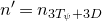 $n' = n_{3 T_{\psi} {+3D}}$
be the constant from Lemma 6.4. If
$n' = n_{3 T_{\psi} {+3D}}$
be the constant from Lemma 6.4. If $j\lt n'$
, then we set
$j\lt n'$
, then we set $u=v=e$
and note that
$u=v=e$
and note that
 \begin{align} \mathsf{d}_\psi (\gamma o, o) &\le \mathsf{d}_\psi(\gamma o, v_j o)+ \mathsf{d}_\psi (v_j o, o) + D \nonumber\\ &\le D_1:= T_\psi + (n' +1)Q_\psi +2D, \end{align}
where $Q_\psi$
is given by Proposition 6.3. Hence the triangle
$Q_\psi$
is given by Proposition 6.3. Hence the triangle $\{uo, vo, \gamma o\}=\{o, o, \gamma o\}$
has
$\{uo, vo, \gamma o\}=\{o, o, \gamma o\}$
has $\mathsf{d}_\psi$
-diameter at most
$\mathsf{d}_\psi$
-diameter at most $D_1$
.
$D_1$
.
Now suppose that $j\gt n'$
. We claim that
$j\gt n'$
. We claim that
 $$\mathsf{d}_\psi(v_{j - n'}o, [\xi, \eta] o) \gt T_{\psi}.$$
Indeed, otherwise, $\mathsf{d}_\psi(v_{j - n'}o, \gamma'o) \le T_{\psi}$
for some
$\mathsf{d}_\psi(v_{j - n'}o, \gamma'o) \le T_{\psi}$
for some $\gamma' \in [\xi, \eta]$
, and hence we have
$\gamma' \in [\xi, \eta]$
, and hence we have
 $$\begin{aligned} \mathsf{d}_{\psi}(o, \gamma' o) & \le \mathsf{d}_{\psi}(o, v_{j - n'} o) + \mathsf{d}_{\psi}( v_{j - n'} o, \gamma' o) {+ D} \\ & \le (\mathsf{d}_{\psi}(o, v_{j} o) - 3 T_{\psi} {- 3 D}) + T_{\psi} {+ D}\\ & = \mathsf{d}_{\psi}(o, v_{j} o) - 2 T_{\psi} {-2 D}\\ & \le \mathsf{d}_{\psi}(o, v_{j} o) - {\mathsf{d}_{\psi}(\gamma o, v_{j}o)} - T_{\psi} {- D}\\ & \le \mathsf{d}_{\psi}(o, \gamma o) - T_{\psi},\end{aligned}$$
where the first and the last inequalities follow from Theorem 4.1 and the second is from Lemma 6.4. This yields a contradiction to the minimality of $\mathsf{d}_{\psi}(o, \gamma o)$
, proving the claim.
$\mathsf{d}_{\psi}(o, \gamma o)$
, proving the claim.
Since the triangle consisting of the sides $[\xi, \eta]o$
,
$[\xi, \eta]o$
, $[e, \xi]o$
, and
$[e, \xi]o$
, and $[e, \eta] o = \{v_i o\}_{i \ge 0}$
is
$[e, \eta] o = \{v_i o\}_{i \ge 0}$
is $T_{\psi}$
-thin, the above claim implies that
$T_{\psi}$
-thin, the above claim implies that $v_{j - n'} o$
lies in the
$v_{j - n'} o$
lies in the $T_{\psi}$
-neighborhood of
$T_{\psi}$
-neighborhood of $[e, \xi] o$
. Hence, there exists
$[e, \xi] o$
. Hence, there exists $u \in [e, \xi]$
such that
$u \in [e, \xi]$
such that $\mathsf{d}_\psi(v_{j-n'} o, u o)\le T_{\psi}$
(see Figure 4). Since
$\mathsf{d}_\psi(v_{j-n'} o, u o)\le T_{\psi}$
(see Figure 4). Since $\mathsf{d}_{\psi}(v_j, v_{j - n'}) \le Q_{\psi} n' + Q_{\psi}$
, we have so far obtained:
$\mathsf{d}_{\psi}(v_j, v_{j - n'}) \le Q_{\psi} n' + Q_{\psi}$
, we have so far obtained:
-
–
$\mathsf{d}_{\psi}(\gamma o, v_j o) \le T_\psi + D $
; -
–
$\mathsf{d}_{\psi}(v_j o, u o) \le Q_{\psi} n' + Q_{\psi} + T_{\psi} + D$
; and -
–
$\mathsf{d}_{\psi}(\gamma o, u o) \le Q_{\psi} n' + Q_{\psi} + 2T_{\psi} + 3D$
.



The choice of $\gamma o$
,
$\gamma o$
, $v_j o$
,
$v_j o$
, $v_{j-n'} o$
and
$v_{j-n'} o$
and $u_k o$
.
$u_k o$
.

Therefore, the triangle $\{uo, v_j o, \gamma o\}$
has
$\{uo, v_j o, \gamma o\}$
has $\mathsf{d}_\psi$
-diameter at most
$\mathsf{d}_\psi$
-diameter at most $D_2 = Q_{\psi} n' + Q_{\psi} + 2T_{\psi} + 3D$
. It remains to set
$D_2 = Q_{\psi} n' + Q_{\psi} + 2T_{\psi} + 3D$
. It remains to set $C=\max (D_1, D_2)$
.
$C=\max (D_1, D_2)$
.
The following has been shown for $\theta = \Pi$
in [Reference Lee and OhLO23, Lemma 5.7], which directly implies the statement for general
$\theta = \Pi$
in [Reference Lee and OhLO23, Lemma 5.7], which directly implies the statement for general $\theta$
.
$\theta$
.
Lemma 6.6.
There exists $\kappa \gt 0$
such that for any
$\kappa \gt 0$
such that for any $g, h \in G$
and
$g, h \in G$
and $R\gt 0$
, we have
$R\gt 0$
, we have
 $$\sup_{\xi \in O^\theta_R(g o, ho)} \| \beta_{\xi}^{\theta}(go, ho) - \mu_{\theta}(g^{-1}h) \| \le \kappa R.$$
We now prove that the $\psi$
-Gromov product
$\psi$
-Gromov product $\psi(\mathcal G(\xi, \eta))$
behaves like the distance
$\psi(\mathcal G(\xi, \eta))$
behaves like the distance $\mathsf{d}_\psi (o, [\xi, \eta] o)$
up to an additive error.
$\mathsf{d}_\psi (o, [\xi, \eta] o)$
up to an additive error.
Proposition 6.7 (Comparison between $\psi$
-Gromov product and
$\psi$
-Gromov product and $\mathsf{d}_{\psi}$
-distance) There exists
$\mathsf{d}_{\psi}$
-distance) There exists $C_1 \gt 0$
such that for any
$C_1 \gt 0$
such that for any $\xi\ne \eta \in \Lambda_{\theta}=\partial \Gamma$
, we have
$\xi\ne \eta \in \Lambda_{\theta}=\partial \Gamma$
, we have
 $$|\psi(\mathcal G^{\theta}(\xi, \eta)) - \mathsf{d}_{\psi}(o, [\xi, \eta] o) | \le C_1.$$
Proof. Let $\gamma\in [\xi, \eta]$
be such that
$\gamma\in [\xi, \eta]$
be such that $\mathsf{d}_{\psi}(o, \gamma o) = \mathsf{d}_{\psi}(o, [\xi, \eta] o)$
. Consider geodesic rays
$\mathsf{d}_{\psi}(o, \gamma o) = \mathsf{d}_{\psi}(o, [\xi, \eta] o)$
. Consider geodesic rays $[e, \xi] $
and
$[e, \xi] $
and $[e, \eta] $
in
$[e, \eta] $
in $(\Gamma, \mathsf{d}_\Gamma)$
. Let
$(\Gamma, \mathsf{d}_\Gamma)$
. Let $k, \ell \in K$
and
$k, \ell \in K$
and $h \in G$
be such that
$h \in G$
be such that $kP_{\theta} = \xi$
,
$kP_{\theta} = \xi$
, $\ell P_{\theta} = \eta$
,
$\ell P_{\theta} = \eta$
, $h P_{\theta}=\xi$
and
$h P_{\theta}=\xi$
and $h w_0 P_{\theta} = \eta$
. For the constant
$h w_0 P_{\theta} = \eta$
. For the constant $D_0$
given by Theorem 4.13, we have
$D_0$
given by Theorem 4.13, we have
 \begin{equation} \begin{aligned} \sup_{u \in [e, \xi]} d(u o, kM_{\theta}A^+ o) &\le D_0; \\ \sup_{v \in [e, \eta]} d(v o, \ell M_{\theta}A^+ o) &\le D_0; \\ \sup_{g \in [\xi, \eta]} d (g o, hM_{\theta} A o) &\le D_0. \end{aligned} \end{equation}
Since $\gamma\in [\xi, \eta]$
by the choice, the third inequality implies that
$\gamma\in [\xi, \eta]$
by the choice, the third inequality implies that $d (\gamma o, hM_\theta A o) \le D_0$
. We may assume that h satisfies that
$d (\gamma o, hM_\theta A o) \le D_0$
. We may assume that h satisfies that $d(h o, \gamma o) \le D_0$
, by replacing h with an element of
$d(h o, \gamma o) \le D_0$
, by replacing h with an element of $hM_{\theta}A$
if necessary.
$hM_{\theta}A$
if necessary.
We first claim that for some uniform $R \gt 0$
depending only on
$R \gt 0$
depending only on $\Gamma$
and
$\Gamma$
and $\psi$
,
$\psi$
,
 $$\xi, \eta \in O_R^{\theta}(o, \gamma o) .$$
To show the claim, let $C \gt 0$
be the constant given by Lemma 6.5 and choose
$C \gt 0$
be the constant given by Lemma 6.5 and choose $u \in [e, \xi]$
and
$u \in [e, \xi]$
and $v \in [e, \eta]$
so that the triangle
$v \in [e, \eta]$
so that the triangle $\{u o, v o, \gamma o\}$
has
$\{u o, v o, \gamma o\}$
has $\mathsf{d}_{\psi}$
-diameter smaller than C (see Figure 5). Hence, for the constant
$\mathsf{d}_{\psi}$
-diameter smaller than C (see Figure 5). Hence, for the constant $C' := C_{\psi}(C + C_{\psi})$
, where
$C' := C_{\psi}(C + C_{\psi})$
, where $C_{\psi}$
is given in (6.2), the Riemannian diameter of the triangle
$C_{\psi}$
is given in (6.2), the Riemannian diameter of the triangle $\{u o, v o, \gamma o\}$
is less than C’. It then follows from the first two inequalities of (6.7) that
$\{u o, v o, \gamma o\}$
is less than C’. It then follows from the first two inequalities of (6.7) that
 $$d(\gamma o, k M_{\theta}A^+ o) \lt D_0 + C' \quad \text{and} \quad d(\gamma o, \ell M_{\theta}A^+ o) \lt D_0 + C'.$$
Since $k P_{\theta} = \xi$
and
$k P_{\theta} = \xi$
and $\ell P_{\theta} = \eta$
, we have
$\ell P_{\theta} = \eta$
, we have
 $$\xi, \eta \in O_{D_0 + C'}^{\theta}(o, \gamma o),$$
showing the claim with $R = D_0 + C'$
Therefore, by Lemma 6.6, we obtain
$R = D_0 + C'$
Therefore, by Lemma 6.6, we obtain
 $$\| \beta_{\xi}^{\theta}(o, \gamma o) - \mu_{\theta}(\gamma) \| \le \kappa R \quad \text{and} \quad \| \beta_{\eta}^{\theta}(o, \gamma o) - \mu_{\theta}(\gamma) \| \le \kappa R.$$
Since $\beta_{\xi}^{\theta}(o, \gamma o) = \beta_{\xi}^{\theta}(o, ho) + \beta_{\xi}^{\theta}(ho, \gamma o)$
and
$\beta_{\xi}^{\theta}(o, \gamma o) = \beta_{\xi}^{\theta}(o, ho) + \beta_{\xi}^{\theta}(ho, \gamma o)$
and $\|\beta_{\xi}^{\theta}(ho, \gamma o) \| \le d(ho, \gamma o) \le D_0$
, we have
$\|\beta_{\xi}^{\theta}(ho, \gamma o) \| \le d(ho, \gamma o) \le D_0$
, we have
 $$\|\beta_{\xi}^{\theta}(o, h o) - \mu_{\theta}(\gamma) \| \le \kappa R + D_0$$
and, similarly,
 $$\|\beta_{\eta}^{\theta}(o, h o) - \mu_{\theta}(\gamma) \| \le \kappa R + D_0.$$
Recalling the definition $\mathcal G^{\theta}(\xi, \eta) =({1}/{2})(\beta_{\xi}^{\theta}(o, ho) + {\rm i}(\beta_{\eta}^{\theta}(o, ho)))$
, and using
$\mathcal G^{\theta}(\xi, \eta) =({1}/{2})(\beta_{\xi}^{\theta}(o, ho) + {\rm i}(\beta_{\eta}^{\theta}(o, ho)))$
, and using $\psi = \psi \circ {\rm i}$
, we obtain that
$\psi = \psi \circ {\rm i}$
, we obtain that
 $$|\psi(\mathcal G^{\theta}(\xi, \eta)) - \mathsf{d}_{\psi}(o, \gamma o) | \le \| \psi \| ( \kappa R + D_0),$$
as desired.
The dotted triangle is of diameter less than C and the gray ball has radius R.

We are now ready to prove the first inclusion in Theorem 6.2, which we formulate again as follows.
Proposition 6.8.
There exist constants $c, R_0 \gt 0$
such that for any
$c, R_0 \gt 0$
such that for any $\xi \in \Lambda_{\theta}$
and
$\xi \in \Lambda_{\theta}$
and $g \in [e,\xi]$
in
$g \in [e,\xi]$
in $\Gamma$
, we have
$\Gamma$
, we have
 \begin{equation} B_{\psi}(\xi, c e^{-\mathsf{d}_{\psi}(o, go)}) \subset O_{R_0}^{\theta}(o, g o) \cap \Lambda_{\theta}.\end{equation}
Proof. Let $C_1, D \gt 0$
be the constants given by Proposition 6.7 and Theorem 4.1, respectively. Recall the constant
$C_1, D \gt 0$
be the constants given by Proposition 6.7 and Theorem 4.1, respectively. Recall the constant $T_{\psi}$
in Proposition 6.3; the image of any geodesic triangle in
$T_{\psi}$
in Proposition 6.3; the image of any geodesic triangle in $(\Gamma, \mathsf{d}_{\Gamma})$
under the orbit map, is
$(\Gamma, \mathsf{d}_{\Gamma})$
under the orbit map, is $T_{\psi}$
-thin in the
$T_{\psi}$
-thin in the $\mathsf{d}_\psi$
-metric. We now claim that (6.8) holds with
$\mathsf{d}_\psi$
-metric. We now claim that (6.8) holds with $c := e^{- (2 T_{\psi} + C_1 + D)} $
. Fix
$c := e^{- (2 T_{\psi} + C_1 + D)} $
. Fix $\xi \in \Lambda_{\theta}$
and an element
$\xi \in \Lambda_{\theta}$
and an element $g\in [e, \xi]$
. Let
$g\in [e, \xi]$
. Let $\eta \in B_{\psi}(\xi, c e^{-\mathsf{d}_{\psi}(o, go)} )$
; that is,
$\eta \in B_{\psi}(\xi, c e^{-\mathsf{d}_{\psi}(o, go)} )$
; that is,
 \begin{equation} \psi(\mathcal G^{\theta}(\xi, \eta)) \gt \mathsf{d}_{\psi}(o, go) + 2 T_{\psi} + C_1 + D.\end{equation}
Let $\gamma \in [\xi, \eta]$
be chosen so that
$\gamma \in [\xi, \eta]$
be chosen so that $\mathsf{d}_{\psi}(o, \gamma o) = \mathsf{d}_{\psi}(o, [\xi, \eta] o)$
. By Proposition 6.7, we have
$\mathsf{d}_{\psi}(o, \gamma o) = \mathsf{d}_{\psi}(o, [\xi, \eta] o)$
. By Proposition 6.7, we have
 $$\mathsf{d}_{\psi}(o, \gamma o) \ge \psi(\mathcal G^{\theta}(\xi, \eta)) - C_1 .$$
Hence, by (6.9),
 \begin{equation} \mathsf{d}_{\psi}(o, \gamma o) \gt \mathsf{d}_{\psi}(o, go) + 2 T_{\psi} + D.\end{equation}
Let $g' \in [\xi, \eta]$
be such that
$g' \in [\xi, \eta]$
be such that $\mathsf{d}_{\psi}(go, g' o) = \mathsf{d}_{\psi}(go, [\xi, \eta] o)$
. By Theorem 4.1, we also have
$\mathsf{d}_{\psi}(go, g' o) = \mathsf{d}_{\psi}(go, [\xi, \eta] o)$
. By Theorem 4.1, we also have
 $$\mathsf{d}_{\psi}(o, \gamma o) \le \mathsf{d}_{\psi}(o, g' o) \le \mathsf{d}_{\psi}(o, g o) + \mathsf{d}_{\psi}(g o, [\xi, \eta] o) + D.$$
Together with (6.10), this implies
 \begin{equation} \mathsf{d}_{\psi}(g o, [\xi, \eta] o) \gt 2 T_{\psi} .\end{equation}
Since the triangle $[e, \xi]o \cup [\xi, \eta]o \cup [e, \eta ]o$
is
$[e, \xi]o \cup [\xi, \eta]o \cup [e, \eta ]o$
is $T_{\psi}$
-thin in
$T_{\psi}$
-thin in $\mathsf{d}_{\psi}$
-metric, go is contained in the
$\mathsf{d}_{\psi}$
-metric, go is contained in the $T_{\psi}$
-neighborhood of
$T_{\psi}$
-neighborhood of $[\xi, \eta]o \cup [e, \eta ]o$
. Since
$[\xi, \eta]o \cup [e, \eta ]o$
. Since $\mathsf{d}_{\psi}(g o, [\xi, \eta] o) \gt 2 T_{\psi}$
by (6.11), we must have
$\mathsf{d}_{\psi}(g o, [\xi, \eta] o) \gt 2 T_{\psi}$
by (6.11), we must have $\mathsf{d}_{\psi}(g o, [e, \eta] o) \le T_{\psi} $
(see Figure 6). For the constant
$\mathsf{d}_{\psi}(g o, [e, \eta] o) \le T_{\psi} $
(see Figure 6). For the constant $T' := C_{\psi}(T_{\psi} + C_{\psi})$
, where
$T' := C_{\psi}(T_{\psi} + C_{\psi})$
, where $C_{\psi}$
is as in (6.2), we have
$C_{\psi}$
is as in (6.2), we have
 $$d(g o, [e, \eta] o) \le T'.$$
With the constant $D_0$
given in Theorem 4.13, there exists
$D_0$
given in Theorem 4.13, there exists $\ell \in K$
so that
$\ell \in K$
so that $\ell P_{\theta} = \eta$
and
$\ell P_{\theta} = \eta$
and $[e, \eta] o$
is contained in the
$[e, \eta] o$
is contained in the $D_0$
-neighborhood of
$D_0$
-neighborhood of $\ell M_{\theta}A^+ o$
in the Riemannian distance d. This implies that
$\ell M_{\theta}A^+ o$
in the Riemannian distance d. This implies that
 $$\eta \in O_{T' + D_0}^{\theta}(o, go)\cap \Lambda_\theta.$$
This completes the proof with $R_0=T'+D_0$
.
$R_0=T'+D_0$
.
go is far from $[\xi, \eta]o$
and hence close to
$[\xi, \eta]o$
and hence close to $[e, \eta]o$
; so
$[e, \eta]o$
; so $\eta$
lies in the shadow
$\eta$
lies in the shadow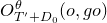 $O^{\theta}_{T' + D_0}(o, go)$
.
$O^{\theta}_{T' + D_0}(o, go)$
.

7. Shadows inside balls: the second inclusion in Theorem 6.2
We continue the setup from § 6. Hence, ${\rm i}(\theta)=\theta$
and
${\rm i}(\theta)=\theta$
and $\psi\in \mathfrak a_\theta^*$
is a linear form such that
$\psi\in \mathfrak a_\theta^*$
is a linear form such that $\psi\gt 0$
on
$\psi\gt 0$
on $\mathcal L-\{0\}$
and
$\mathcal L-\{0\}$
and $\psi=\psi \circ {\rm i}$
. In this section, we prove the second inclusion of Theorem 6.2, which can be stated as follows.
$\psi=\psi \circ {\rm i}$
. In this section, we prove the second inclusion of Theorem 6.2, which can be stated as follows.
Proposition 7.1.
For any $r \gt 0$
, there exists
$r \gt 0$
, there exists $c' = c'_r \gt 0$
such that for any
$c' = c'_r \gt 0$
such that for any $\xi \in \Lambda_{\theta}$
and any
$\xi \in \Lambda_{\theta}$
and any $g \in [e,\xi]$
in
$g \in [e,\xi]$
in $\Gamma$
, we have
$\Gamma$
, we have
 $$O_r^{\theta}(o, g o) \cap \Lambda_{\theta} \subset B_{\psi}(\xi, c' e^{-\mathsf{d}_{\psi}(o, go)}).$$
In addition to the coarse triangle inequality of $\mathsf{d}_\psi$
(Theorem 4.1) and the uniform progression lemma (Lemma 6.4), we will use the property that the shadows in
$\mathsf{d}_\psi$
(Theorem 4.1) and the uniform progression lemma (Lemma 6.4), we will use the property that the shadows in $(\Gamma, \mathsf{d}_\Gamma)$
are comparable to shadows in
$(\Gamma, \mathsf{d}_\Gamma)$
are comparable to shadows in $\Lambda_\theta$
(Proposition 7.2) and that the half-spaces spanned by shadows of balls in
$\Lambda_\theta$
(Proposition 7.2) and that the half-spaces spanned by shadows of balls in $(\Gamma, \mathsf{d}_{\Gamma})$
stay deeper than the balls from the viewpoints (see Figure 7 and Lemma 7.4).
$(\Gamma, \mathsf{d}_{\Gamma})$
stay deeper than the balls from the viewpoints (see Figure 7 and Lemma 7.4).
A pictorial description of Lemma 7.4.

In the Gromov hyperbolic space $(\Gamma,\mathsf{d}_\Gamma)$
, for
$(\Gamma,\mathsf{d}_\Gamma)$
, for $R\gt 0$
and
$R\gt 0$
and $\gamma_1, \gamma_2\in \Gamma$
, the shadow
$\gamma_1, \gamma_2\in \Gamma$
, the shadow $O_R^{\Gamma}(\gamma_1, \gamma_2)$
is defined as the set of all
$O_R^{\Gamma}(\gamma_1, \gamma_2)$
is defined as the set of all $\xi\in \partial \Gamma$
such that a geodesic ray
$\xi\in \partial \Gamma$
such that a geodesic ray $[\gamma_1, \xi]$
intersects the R-ball centered at
$[\gamma_1, \xi]$
intersects the R-ball centered at $\gamma_2$
:
$\gamma_2$
:
 $$ O_R^{\Gamma}(\gamma_1, \gamma_2)=\{\xi\in \partial \Gamma: \mathsf{d}_\Gamma (\gamma_2, [\gamma_1, \xi])\lt R\} . $$
Clearly, shadows are $\Gamma$
-equivariant in the sense that for any
$\Gamma$
-equivariant in the sense that for any $\gamma\in \Gamma$
, we have
$\gamma\in \Gamma$
, we have $\gamma O_R^{\Gamma}(\gamma_1, \gamma_2)=O_R^{\Gamma}(\gamma \gamma_1, \gamma \gamma_2)$
.
$\gamma O_R^{\Gamma}(\gamma_1, \gamma_2)=O_R^{\Gamma}(\gamma \gamma_1, \gamma \gamma_2)$
.
The following proposition states that shadows in $\partial \Gamma$
and shadows in
$\partial \Gamma$
and shadows in $\Lambda_{\theta}$
are compatible via the boundary map
$\Lambda_{\theta}$
are compatible via the boundary map $f : \partial \Gamma \to \Lambda_{\theta}$
: recall that the orbit map
$f : \partial \Gamma \to \Lambda_{\theta}$
: recall that the orbit map $(\Gamma, \mathsf{d}_{\Gamma}) \to (\Gamma o, d)$
is a Q-quasi-isometry for some
$(\Gamma, \mathsf{d}_{\Gamma}) \to (\Gamma o, d)$
is a Q-quasi-isometry for some $Q \ge 1$
(Theorem 3.8(3)) and let
$Q \ge 1$
(Theorem 3.8(3)) and let $R_0 := Q + D_0 + 1$
, where
$R_0 := Q + D_0 + 1$
, where $D_0$
is given in Theorem 4.13.
$D_0$
is given in Theorem 4.13.
Proposition 7.2.
For any $R\gt R_0$
, there exists
$R\gt R_0$
, there exists $R_1, R_2 \gt 0$
such that for any
$R_1, R_2 \gt 0$
such that for any $\gamma_1, \gamma_2 \in \Gamma$
,
$\gamma_1, \gamma_2 \in \Gamma$
,
 $$f(O_{R_1}^{\Gamma}(\gamma_1, \gamma_2)) \subset O_R^{\theta} (\gamma_1 o, \gamma_2 o) \cap \Lambda_{\theta} \subset f(O_{R_2}^{\Gamma}(\gamma_1, \gamma_2)).$$
In proving this proposition, we also need to consider shadows whose viewpoints are on the boundary $\mathcal F_\theta$
. For
$\mathcal F_\theta$
. For $\eta\in \mathcal F_\theta$
,
$\eta\in \mathcal F_\theta$
, $p\in X$
, and
$p\in X$
, and $R\gt 0$
, the
$R\gt 0$
, the $\theta$
-shadow
$\theta$
-shadow $O_R^{\theta}(\eta, p)$
is defined as follows:
$O_R^{\theta}(\eta, p)$
is defined as follows:
 $$O_R^{\theta}(\eta, p) = \{g P_{\theta} \in \mathcal F_{\theta} : g \in G, gw_0P_{\theta} = \eta, d(p, go)\lt R \}.$$
We need the following proposition on continuity of shadows.
Proposition 7.3 (Continuity of shadows on viewpoints [Reference Kim, Oh and WangKOW25a, Proposition 3.4]). Let $p \in X$
,
$p \in X$
, $\eta \in \mathcal F_{\theta}$
and
$\eta \in \mathcal F_{\theta}$
and $r\gt 0$
. If a sequence
$r\gt 0$
. If a sequence $q_i \in X$
converges to
$q_i \in X$
converges to $ \eta $
as
$ \eta $
as $i \to \infty$
as in Definition 2.2, then for any
$i \to \infty$
as in Definition 2.2, then for any $0\lt \varepsilon\lt r$
, we have
$0\lt \varepsilon\lt r$
, we have
 \begin{equation} O_{r - \varepsilon}^{\theta}(\eta, p) \subset O_r^{\theta}(q_i, p) \subset O_{r + \varepsilon}^{\theta}(\eta, p) \quad \text{for all large } i\ge 1. \end{equation}
7.1 Proof of Proposition 7.2
Let $R\gt R_0$
. By the
$R\gt R_0$
. By the $\Gamma$
-equivariance of f as well as of shadows, we may assume that
$\Gamma$
-equivariance of f as well as of shadows, we may assume that $\gamma_1 = e$
and write
$\gamma_1 = e$
and write $\gamma_2 = \gamma$
. By applying Theorem 4.13(2), we obtain that for any
$\gamma_2 = \gamma$
. By applying Theorem 4.13(2), we obtain that for any $\xi \in \partial \Gamma$
and
$\xi \in \partial \Gamma$
and $k\in K$
with
$k\in K$
with $kP_{\theta} =f(\xi)$
, the image
$kP_{\theta} =f(\xi)$
, the image $[e, \xi]o$
is contained in the
$[e, \xi]o$
is contained in the $D_0$
-neighborhood of
$D_0$
-neighborhood of $kM_\theta (\exp \mathcal C) o\subset k M_{\theta} A^+ o$
in the symmetric space (X, d). Since
$kM_\theta (\exp \mathcal C) o\subset k M_{\theta} A^+ o$
in the symmetric space (X, d). Since $R\gt R_0=Q+D_0+1 $
, we can choose
$R\gt R_0=Q+D_0+1 $
, we can choose $R_1\gt 0$
so that
$R_1\gt 0$
so that $ Q R_1+ Q+D_0 \lt R$
. Now if
$ Q R_1+ Q+D_0 \lt R$
. Now if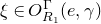 $\xi\in O^\Gamma_{R_1}(e, \gamma)$
, and hence
$\xi\in O^\Gamma_{R_1}(e, \gamma)$
, and hence $[e, \xi]$
intersects the ball
$[e, \xi]$
intersects the ball $\{g\in \Gamma: \mathsf{d}_\Gamma( \gamma , g)\lt R_1\}$
, then
$\{g\in \Gamma: \mathsf{d}_\Gamma( \gamma , g)\lt R_1\}$
, then $kM_{\theta}A^+ o$
intersects the
$kM_{\theta}A^+ o$
intersects the $ Q R_1+ Q+D_0 $
-neighborhood of
$ Q R_1+ Q+D_0 $
-neighborhood of $\gamma o$
, and hence the R-neighborhood of
$\gamma o$
, and hence the R-neighborhood of $\gamma o$
. Therefore,
$\gamma o$
. Therefore, $f(\xi) \in O_{R}^{\theta}(o, \gamma o)$
. This shows the first inclusion.
$f(\xi) \in O_{R}^{\theta}(o, \gamma o)$
. This shows the first inclusion.
To prove the second inclusion, suppose that the claim does not hold for some $R\gt R_0$
. Then, for each
$R\gt R_0$
. Then, for each $i \ge 1$
, there exists
$i \ge 1$
, there exists $\gamma_i \in \Gamma$
such that
$\gamma_i \in \Gamma$
such that
 $$O_R^{\theta}(o, \gamma_i o) \cap \Lambda_{\theta} \not \subset f(O_i^{\Gamma}(e, \gamma_i));$$
in other words, there exists $x_i \in \partial \Gamma - O_i^{\Gamma}(e, \gamma_i)$
such that
$x_i \in \partial \Gamma - O_i^{\Gamma}(e, \gamma_i)$
such that $f(x_i) \in O_R^{\theta}(o, \gamma_i o)$
. By the
$f(x_i) \in O_R^{\theta}(o, \gamma_i o)$
. By the $\Gamma$
-equivariance of f, it follows that
$\Gamma$
-equivariance of f, it follows that
 $$\gamma_i^{-1}x_i \notin O_i^{\Gamma}(\gamma_i^{-1}, e) \quad \text{and} \quad f(\gamma_i^{-1}x_i) \in O_R^{\theta}(\gamma_i^{-1} o, o) \quad \text{for all } i \ge 1.$$
After passing to a subsequence, we may assume that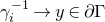 $\gamma_i^{-1} \to y \in \partial \Gamma$
and
$\gamma_i^{-1} \to y \in \partial \Gamma$
and $\gamma_i^{-1}x_i \to x$
as
$\gamma_i^{-1}x_i \to x$
as $i \to \infty$
. By Theorem 3.8(4), we deduce
$i \to \infty$
. By Theorem 3.8(4), we deduce $\gamma_i^{-1} o \to f(y)$
as
$\gamma_i^{-1} o \to f(y)$
as $i \to \infty$
. Applying Proposition 7.3 to
$i \to \infty$
. Applying Proposition 7.3 to $q_i = \gamma_i^{-1} o$
,
$q_i = \gamma_i^{-1} o$
, $p = o$
and
$p = o$
and $\eta = f(y)$
, we have for some
$\eta = f(y)$
, we have for some $\varepsilon \gt 0$
that
$\varepsilon \gt 0$
that
 $$ O_{R}^{\theta}(\gamma_i^{-1}o, o) \subset O_{R + \varepsilon/2}^{\theta}(f(y), o) \quad \text{for all } i \ge 1.$$
Since $f(\gamma_i^{-1} x_i) \in O_{R}^{\theta}(\gamma_i^{-1}o, o)$
for all
$f(\gamma_i^{-1} x_i) \in O_{R}^{\theta}(\gamma_i^{-1}o, o)$
for all $i \ge 1$
and
$i \ge 1$
and $f(\gamma_i^{-1} x_i) $
converges to f(x) as
$f(\gamma_i^{-1} x_i) $
converges to f(x) as $i \to \infty$
, we have
$i \to \infty$
, we have
 $$f(x) \in O_{R + \varepsilon}^{\theta}(f(y), o).$$
This implies that f(x) is in general position with f(y), i.e., $(f(x), f(y))\in \mathcal F_\theta^{(2)}$
, and in particular
$(f(x), f(y))\in \mathcal F_\theta^{(2)}$
, and in particular $f(x) \neq f(y)$
. On the other hand, since
$f(x) \neq f(y)$
. On the other hand, since $\gamma_i^{-1}x_i \notin O_i^{\Gamma}(\gamma_i^{-1}, e)$
for all
$\gamma_i^{-1}x_i \notin O_i^{\Gamma}(\gamma_i^{-1}, e)$
for all $i \ge 1$
, the sequence of geodesics
$i \ge 1$
, the sequence of geodesics $[\gamma_i^{-1} x_i, \gamma_i^{-1}]$
escapes any large ball centered at e. This implies that two sequences
$[\gamma_i^{-1} x_i, \gamma_i^{-1}]$
escapes any large ball centered at e. This implies that two sequences $\gamma_i^{-1} x_i$
and
$\gamma_i^{-1} x_i$
and $\gamma_i^{-1}$
must have the same limit, and hence
$\gamma_i^{-1}$
must have the same limit, and hence $x = y$
, which is a contradiction. Therefore, the claim follows.
$x = y$
, which is a contradiction. Therefore, the claim follows.
The Gromov product in $(\Gamma, \mathsf{d}_{\Gamma})$
is defined as follows: for
$(\Gamma, \mathsf{d}_{\Gamma})$
is defined as follows: for $\alpha, \beta, \gamma \in \Gamma$
,
$\alpha, \beta, \gamma \in \Gamma$
,
 $$(\alpha, \beta)_{\gamma} = \tfrac{1}{2} \left( \mathsf{d}_{\Gamma}(\alpha, \gamma) + \mathsf{d}_{\Gamma}(\beta, \gamma) - \mathsf{d}_{\Gamma}(\alpha, \beta)\right)$$
and for $x, y \in \partial \Gamma$
,
$x, y \in \partial \Gamma$
,
 $$(x, y)_{\gamma} = \sup \liminf_{i, j \to \infty} (x_i,y_j)_{\gamma}$$
where the supremum is taken over all sequences $\{x_i\}, \{y_j\}$
in
$\{x_i\}, \{y_j\}$
in $\Gamma$
such that
$\Gamma$
such that $\lim_{i \to \infty} x_i = x$
and
$\lim_{i \to \infty} x_i = x$
and $\lim_{j \to \infty} y_j = y$
. The Gromov product for a pair of a point in
$\lim_{j \to \infty} y_j = y$
. The Gromov product for a pair of a point in $\Gamma$
and a point in
$\Gamma$
and a point in $\partial \Gamma$
is defined similarly. The Gromov product
$\partial \Gamma$
is defined similarly. The Gromov product $(x, y)_{\gamma}$
is known to measure distance from
$(x, y)_{\gamma}$
is known to measure distance from $\gamma$
and to a geodesic [x, y] up to a uniform additive error (for basic properties of Gromov hyperbolic spaces, see [Reference Bridson and HaefligerBH99]).
$\gamma$
and to a geodesic [x, y] up to a uniform additive error (for basic properties of Gromov hyperbolic spaces, see [Reference Bridson and HaefligerBH99]).
The following lemma says that the half-space spanned by the shadow is opposite to the light; more precisely, for any $x\in \partial \Gamma$
and
$x\in \partial \Gamma$
and $\gamma\in [e,x]$
, the half-space spanned by all geodesics connecting x and
$\gamma\in [e,x]$
, the half-space spanned by all geodesics connecting x and $O^\Gamma_R(e,\gamma)$
lies farther than
$O^\Gamma_R(e,\gamma)$
lies farther than $\gamma$
, viewed from e.
$\gamma$
, viewed from e.
Lemma 7.4.
Given $R \gt 0$
, there exists
$R \gt 0$
, there exists $r = r_R \gt 0$
such that for any
$r = r_R \gt 0$
such that for any $x\in \partial \Gamma$
,
$x\in \partial \Gamma$
, $\gamma\in [e,x]$
, and
$\gamma\in [e,x]$
, and $y \in O_R^{\Gamma}(e, \gamma)$
, we have
$y \in O_R^{\Gamma}(e, \gamma)$
, we have
 $$\mathsf{d}_{\Gamma}(\gamma_{x,y}, [\gamma, x] ) \le r,$$
where $\gamma_{x,y}\in [x, y]$
denotes the nearest-point projection of e to a geodesic [x,y].
$\gamma_{x,y}\in [x, y]$
denotes the nearest-point projection of e to a geodesic [x,y].
Proof. Let $[e, x] = \{\gamma_i\}_{i \ge 0}$
. We fix
$[e, x] = \{\gamma_i\}_{i \ge 0}$
. We fix $\gamma := \gamma_i$
and
$\gamma := \gamma_i$
and $y \in O_R^{\Gamma}(e, \gamma)$
. In terms of the Gromov product, we have
$y \in O_R^{\Gamma}(e, \gamma)$
. In terms of the Gromov product, we have $(e, y)_{\gamma} \lt R + \delta / 2$
for some uniform
$(e, y)_{\gamma} \lt R + \delta / 2$
for some uniform $\delta \gt 0$
depending only on
$\delta \gt 0$
depending only on $\Gamma$
. On the other hand, the hyperbolicity of
$\Gamma$
. On the other hand, the hyperbolicity of $\Gamma$
also implies that we can take
$\Gamma$
also implies that we can take $\delta$
large enough so that
$\delta$
large enough so that
 $$(e, y)_{\gamma} \ge \min \{(e, \gamma_{x,y})_{\gamma}, (\gamma_{x,y}, y)_{\gamma} \} - \delta/2$$
and that every geodesic triangle in $\Gamma \cup \partial \Gamma$
is
$\Gamma \cup \partial \Gamma$
is $\delta$
-thin. Therefore
$\delta$
-thin. Therefore
 $$\min \{(e, \gamma_{x,y})_{\gamma}, (\gamma_{x,y}, y)_{\gamma} \} \lt R+\delta .$$
First, consider the case when $(\gamma_{x,y}, y)_{\gamma} \lt R + \delta$
. Then, for some constant
$(\gamma_{x,y}, y)_{\gamma} \lt R + \delta$
. Then, for some constant $\delta_1$
depending on
$\delta_1$
depending on $R + \delta$
, there exists
$R + \delta$
, there exists $\gamma' \in [\gamma_{x,y}, y]$
such that
$\gamma' \in [\gamma_{x,y}, y]$
such that $\mathsf{d}_{\Gamma}(\gamma', \gamma) \lt \delta_1$
. Consider the geodesic triangle with vertices
$\mathsf{d}_{\Gamma}(\gamma', \gamma) \lt \delta_1$
. Consider the geodesic triangle with vertices $x, \gamma, \gamma'$
. Since this triangle is
$x, \gamma, \gamma'$
. Since this triangle is $\delta$
-thin and
$\delta$
-thin and $\gamma_{x,y} \in [x, \gamma']$
, the
$\gamma_{x,y} \in [x, \gamma']$
, the $\delta$
-neighborhood of
$\delta$
-neighborhood of $\gamma_{x,y}$
intersects
$\gamma_{x,y}$
intersects $[x, \gamma] \cup [\gamma, \gamma']$
. Hence it follows from
$[x, \gamma] \cup [\gamma, \gamma']$
. Hence it follows from $\mathsf{d}_{\Gamma}(\gamma, \gamma') \lt \delta_1$
that the
$\mathsf{d}_{\Gamma}(\gamma, \gamma') \lt \delta_1$
that the $(\delta + \delta_1)$
-neighborhood of
$(\delta + \delta_1)$
-neighborhood of $\gamma_{x,y}$
intersects the geodesic
$\gamma_{x,y}$
intersects the geodesic $[x, \gamma]$
. Namely,
$[x, \gamma]$
. Namely,
 $$\mathsf{d}_{\Gamma}(\gamma_{x,y}, [\gamma, x] ) \le \delta+\delta_1.$$
Now consider the case that $(e, \gamma_{x,y})_{\gamma} \lt R + \delta$
. Since
$(e, \gamma_{x,y})_{\gamma} \lt R + \delta$
. Since $\gamma_{x,y}$
is the nearest-point projection of e to [x, y], there exists a constant
$\gamma_{x,y}$
is the nearest-point projection of e to [x, y], there exists a constant $\delta_2$
depending only on
$\delta_2$
depending only on $\Gamma$
such that the
$\Gamma$
such that the $\delta_2$
-neighborhood of
$\delta_2$
-neighborhood of $\gamma_{x,y}$
intersects both geodesic rays [e, x] and [e, y]. In particular, there exists
$\gamma_{x,y}$
intersects both geodesic rays [e, x] and [e, y]. In particular, there exists $\gamma_{k}\in [e, x]$
such that
$\gamma_{k}\in [e, x]$
such that $\mathsf{d}_{\Gamma}(\gamma_{x,y}, \gamma_{k}) \lt \delta_2$
. This implies
$\mathsf{d}_{\Gamma}(\gamma_{x,y}, \gamma_{k}) \lt \delta_2$
. This implies
 $$(e, \gamma_{k})_{\gamma} \le (e, \gamma_{x,y})_{\gamma} + \mathsf{d}_{\Gamma}(\gamma_{x,y}, \gamma_{k}) \lt R + \delta + \delta_2.$$
Since both $\gamma =\gamma_i $
and
$\gamma =\gamma_i $
and $ \gamma_{k}$
lie on the geodesic [e, x], this implies that
$ \gamma_{k}$
lie on the geodesic [e, x], this implies that ${k} \ge i - (R + \delta + \delta_2)$
. Let j be the unique integer such that
${k} \ge i - (R + \delta + \delta_2)$
. Let j be the unique integer such that $k + R + \delta + \delta_2 \le j \le k + R + \delta + \delta_2 + 1$
. Note that since
$k + R + \delta + \delta_2 \le j \le k + R + \delta + \delta_2 + 1$
. Note that since $k \ge i - (R + \delta + \delta_2)$
, we have
$k \ge i - (R + \delta + \delta_2)$
, we have $j \ge i$
, and hence
$j \ge i$
, and hence $\gamma_j \in [\gamma, x]$
. Then,
$\gamma_j \in [\gamma, x]$
. Then,
 \begin{align*} \mathsf{d}_{\Gamma}(\gamma_{x,y}, [\gamma, x] ) &\le \mathsf{d}_{\Gamma}(\gamma_{x,y}, \gamma_j) \\ &\le \mathsf{d}_{\Gamma}(\gamma_{x, y}, \gamma_k) + \mathsf{d}_{\Gamma}(\gamma_k, \gamma_j) \\ &\le \delta_2 + (j-k)\le R + \delta + 2 \delta_2 + 1 . \end{align*}
Therefore, it remains to set $r = R + \delta + \delta_1 + 2 \delta_2 + 1$
.
$r = R + \delta + \delta_1 + 2 \delta_2 + 1$
.
We are new ready to prove Proposition 7.1.
7.2 Proof of Proposition 7.1
Let $\xi \in \Lambda_\theta=\partial\Gamma$
and
$\xi \in \Lambda_\theta=\partial\Gamma$
and $g\in [e,\xi]$
in
$g\in [e,\xi]$
in $\Gamma$
. Fix
$\Gamma$
. Fix $r\gt 0$
, and let
$r\gt 0$
, and let $\eta \in O_r^{\theta}(o, g o) \cap \Lambda_{\theta}$
distinct from
$\eta \in O_r^{\theta}(o, g o) \cap \Lambda_{\theta}$
distinct from $\xi$
. We will continue to use the convention of identifying
$\xi$
. We will continue to use the convention of identifying $\Lambda_\theta$
and
$\Lambda_\theta$
and $\partial \Gamma$
in this proof. As in Lemma 7.4, we let
$\partial \Gamma$
in this proof. As in Lemma 7.4, we let $\gamma_{\xi,\eta}$
be the nearest-point projection of e to a bi-infinite geodesic
$\gamma_{\xi,\eta}$
be the nearest-point projection of e to a bi-infinite geodesic $[\xi, \eta]$
in
$[\xi, \eta]$
in $(\Gamma, \mathsf{d}_\Gamma)$
. By Proposition 7.2, there exists
$(\Gamma, \mathsf{d}_\Gamma)$
. By Proposition 7.2, there exists $R\gt 0$
, depending only on r, such that
$R\gt 0$
, depending only on r, such that $\eta \in O_R^{\Gamma}(e, g)$
. Write the geodesic ray
$\eta \in O_R^{\Gamma}(e, g)$
. Write the geodesic ray $[e,\xi]$
as a sequence
$[e,\xi]$
as a sequence $\{g_k\}_{k \ge 0}$
with
$\{g_k\}_{k \ge 0}$
with $g_0=e$
. Since
$g_0=e$
. Since $g\in [e,\xi]$
by the hypothesis, we have
$g\in [e,\xi]$
by the hypothesis, we have $g_i = g$
for some
$g_i = g$
for some $i \ge 0$
. Then, for
$i \ge 0$
. Then, for $r_R \gt 0$
given in Lemma 7.4, there exists
$r_R \gt 0$
given in Lemma 7.4, there exists $j \ge i$
such that
$j \ge i$
such that
 $$\mathsf{d}_{\Gamma}(\gamma_{\xi,\eta}, g_j) \le r_R.$$
Let $n_1 \ge 0$
and
$n_1 \ge 0$
and $D \ge 0$
be given by Lemma 6.4 (uniform progression lemma) and Theorem 4.1 (coarse triangle inequality), respectively. We then have
$D \ge 0$
be given by Lemma 6.4 (uniform progression lemma) and Theorem 4.1 (coarse triangle inequality), respectively. We then have
 $$\begin{aligned} \mathsf{d}_{\psi}(o, g_j o) & \ge \mathsf{d}_{\psi}(o, g_{i - n_1} o) + 1 \\ & \ge \mathsf{d}_{\psi}(o, g o) - \mathsf{d}_{\psi}(g_{i - n_1} o, g o) - D + 1 \end{aligned} .$$
Since $g = g_i$
, we have
$g = g_i$
, we have $\mathsf{d}_{\psi}(g_{i - n_1} o, go) \le Q_{\psi}(n_1 + 1)$
, where
$\mathsf{d}_{\psi}(g_{i - n_1} o, go) \le Q_{\psi}(n_1 + 1)$
, where $Q_{\psi}$
is the constant in Proposition 6.3. Hence we deduce by setting
$Q_{\psi}$
is the constant in Proposition 6.3. Hence we deduce by setting $D' := Q_{\psi}(n_1 + 1) + D$
that
$D' := Q_{\psi}(n_1 + 1) + D$
that
 $$\mathsf{d}_{\psi}(o, g_j o) \ge \mathsf{d}_{\psi}(o, g o ) - D'.$$
On the other hand, applying the coarse triangle inequality (Theorem 4.1) again, we have
 $$\mathsf{d}_{\psi}(o, g_j o) \le \mathsf{d}_{\psi}(o, \gamma_{\xi,\eta} o) + \mathsf{d}_{\psi}(\gamma_{\xi,\eta} o, g_j o) + D.$$
Since $\mathsf{d}_{\Gamma}(\gamma_{\xi,\eta}, g_j) \le r_R$
, we have
$\mathsf{d}_{\Gamma}(\gamma_{\xi,\eta}, g_j) \le r_R$
, we have $\mathsf{d}_{\psi}(\gamma_{\xi,\eta} o, g_j o) \le Q_{\psi}(r_R + 1)$
by Proposition 6.3, and hence
$\mathsf{d}_{\psi}(\gamma_{\xi,\eta} o, g_j o) \le Q_{\psi}(r_R + 1)$
by Proposition 6.3, and hence
 $$\mathsf{d}_{\psi}(o, \gamma_{\xi,\eta} o) \ge \mathsf{d}_{\psi}(o, go) - D' - Q_{\psi}(r_R + 1) - D.$$
Since we have $|\psi( \mathcal G^{\theta}(\xi, \eta)) - \mathsf{d}_{\psi}(o, \gamma_{\xi,\eta} o) | \lt \|\psi\|C_1$
with
$|\psi( \mathcal G^{\theta}(\xi, \eta)) - \mathsf{d}_{\psi}(o, \gamma_{\xi,\eta} o) | \lt \|\psi\|C_1$
with $C_1$
given by Lemma 5.4,
$C_1$
given by Lemma 5.4,
 $$\psi( \mathcal G^{\theta}(\xi, \eta)) \ge \mathsf{d}_{\psi}(o, go) - D' - Q_{\psi}(r_R + 1) - D - \|\psi\|C_1 .$$
Setting $c' := e^{D' + Q_{\psi}(r_R + 1) + D + \|\psi\|C_1}$
, we have
$c' := e^{D' + Q_{\psi}(r_R + 1) + D + \|\psi\|C_1}$
, we have
 $$d_{\psi}(\xi, \eta) \le c' e^{-\mathsf{d}_{\psi}(o, go)}.$$
Hence $\eta \in B_\psi (\xi, c' e^{{-\mathsf{d}_{\psi}(o, go)}}) $
as desired.
$\eta \in B_\psi (\xi, c' e^{{-\mathsf{d}_{\psi}(o, go)}}) $
as desired.
7.3 Comparing Gromov products
Lemma 7.5.
Let $\psi \in \mathfrak a_{\theta}^*$
be such that
$\psi \in \mathfrak a_{\theta}^*$
be such that $\psi \gt 0$
on
$\psi \gt 0$
on $\mathcal L - \{0\}$
. Then there exists
$\mathcal L - \{0\}$
. Then there exists $c \gt 0$
, depending only on
$c \gt 0$
, depending only on $\psi$
, such that for all
$\psi$
, such that for all $x, y\in \partial\Gamma$
,
$x, y\in \partial\Gamma$
,
 $$ Q_{\bar \psi}^{-1} \cdot (x, y)_e - c \le \psi(\mathcal G^{\theta}(f(x), f(y))) \le Q_{\bar \psi} \cdot (x, y)_e + c,$$
where $Q_{\bar\psi}$
is as given in Proposition 6.3.
$Q_{\bar\psi}$
is as given in Proposition 6.3.
Proof. Let $x \neq y \in \partial \Gamma$
and set
$x \neq y \in \partial \Gamma$
and set $\gamma_{x, y} \in \Gamma$
the nearest-point projection of e to [x, y] in
$\gamma_{x, y} \in \Gamma$
the nearest-point projection of e to [x, y] in $(\Gamma, \mathsf{d}_{\Gamma})$
. By Lemma 5.4, we have
$(\Gamma, \mathsf{d}_{\Gamma})$
. By Lemma 5.4, we have
 $$| \bar \psi( \mathcal G^{\theta}(f(x), f(y))) - \bar \psi(\mu_{\theta}(\gamma_{x, y}))| \lt C_1$$
where $C_1$
is given in Lemma 5.4. As in the proof of Proposition 5.5,
$C_1$
is given in Lemma 5.4. As in the proof of Proposition 5.5,
 $$| \bar \psi( \mathcal G^{\theta}(f(x), f(y))) - \psi( \mathcal G^{\theta}(f(x), f(y)))| \lt \| \psi \| C_1.$$
Since
 $$Q_{\bar \psi}^{-1} \cdot \mathsf{d}_{\Gamma}(e, \gamma_{x, y}) - Q_{\bar \psi} \le \bar \psi(\mu_{\theta}(\gamma_{x, y})) \le Q_{\bar \psi} \cdot \mathsf{d}_{\Gamma}(e, \gamma_{x, y}) + Q_{\bar \psi} $$
by Proposition 6.3 with $Q_{\bar \psi} \ge 1$
therein, we now have that
$Q_{\bar \psi} \ge 1$
therein, we now have that
 $$Q_{\bar \psi}^{-1} \cdot \mathsf{d}_{\Gamma}(e, \gamma_{x, y})- c' \le \psi( \mathcal G^{\theta}(f(x), f(y))) \le Q_{\bar \psi} \cdot \mathsf{d}_{\Gamma}(e, \gamma_{x, y}) +c'$$
where $c' := Q_{\bar \psi} + C_1 (1 + \|\psi\|)$
. Since
$c' := Q_{\bar \psi} + C_1 (1 + \|\psi\|)$
. Since $(\Gamma, \mathsf{d}_{\Gamma})$
is Gromov hyperbolic, we have that
$(\Gamma, \mathsf{d}_{\Gamma})$
is Gromov hyperbolic, we have that $|(x, y)_e - \mathsf{d}_{\Gamma}(e, \gamma_{x, y})|$
is uniformly bounded. Hence, the claim follows.
$|(x, y)_e - \mathsf{d}_{\Gamma}(e, \gamma_{x, y})|$
is uniformly bounded. Hence, the claim follows.
8. Ahlfors regularity of Patterson–Sullivan measures
As before, let $\Gamma$
be a
$\Gamma$
be a $\theta$
-Anosov subgroup of a connected semisimple real algebraic group G. Recall from Theorem 3.4 that the space of
$\theta$
-Anosov subgroup of a connected semisimple real algebraic group G. Recall from Theorem 3.4 that the space of $\Gamma$
-Patterson–Sullivan measures on
$\Gamma$
-Patterson–Sullivan measures on $\Lambda_\theta$
is parameterized by the set
$\Lambda_\theta$
is parameterized by the set
 $$ \mathscr T_\Gamma=\{\psi\in \mathfrak a_\theta^*: \psi \text{ is tangent to } \psi_\Gamma^\theta \}. $$
We continue to use the notation $\nu_\psi$
for the unique
$\nu_\psi$
for the unique $(\Gamma, \psi)$
-Patterson–Sullivan measure on
$(\Gamma, \psi)$
-Patterson–Sullivan measure on $\Lambda_{\theta}$
. Recall that
$\Lambda_{\theta}$
. Recall that $d_\psi $
is the premetric on
$d_\psi $
is the premetric on $\Lambda_\theta$
defined by
$\Lambda_\theta$
defined by $d_\psi(\xi, \eta)=e^{-\psi(\mathcal G(\xi, \eta))}$
for all
$d_\psi(\xi, \eta)=e^{-\psi(\mathcal G(\xi, \eta))}$
for all $\xi\ne \eta$
in
$\xi\ne \eta$
in $\Lambda_\theta$
and
$\Lambda_\theta$
and $B_{\psi}(\xi, r)=\{\eta\in \Lambda_\theta: d_\psi(\xi, \eta)\lt r\}$
.
$B_{\psi}(\xi, r)=\{\eta\in \Lambda_\theta: d_\psi(\xi, \eta)\lt r\}$
.
The Ahlfors regularity is an important notion in fractal geometry.
Definition 8.1.
A premetric space (Z, d) is called Ahlfors s-regular if there exist a Borel measure $\nu$
on Z and
$\nu$
on Z and $C\ge 1$
so that for all
$C\ge 1$
so that for all $z\in Z$
and
$z\in Z$
and $r\in [0, \operatorname{{\rm diam}} Z)$
,
$r\in [0, \operatorname{{\rm diam}} Z)$
,
 $$C^{-1} r^s \le \nu (B(z,r)) \le C r^s,$$
where $B(z, r)=\{w\in Z: d(z,w)\lt r\}$
. Such a measure
$B(z, r)=\{w\in Z: d(z,w)\lt r\}$
. Such a measure $\nu$
is also called Ahlfors s-regular.
$\nu$
is also called Ahlfors s-regular.
The goal of this section is to deduce the following from Theorem 6.2.
Theorem 8.2.
For any symmetric $\psi \in \mathscr T_\Gamma$
, the measure
$\psi \in \mathscr T_\Gamma$
, the measure $\nu_\psi$
is Ahlfors one-regular on
$\nu_\psi$
is Ahlfors one-regular on $(\Lambda_\theta, d_\psi)$
.
$(\Lambda_\theta, d_\psi)$
.
Remark 8.3. When $\Gamma$
is a convex cocompact subgroup of
$\Gamma$
is a convex cocompact subgroup of $G=\operatorname{{\rm SO}}^\circ (n,1)$
,
$G=\operatorname{{\rm SO}}^\circ (n,1)$
, $\mathscr T_\Gamma$
is a singleton consisting of the critical exponent
$\mathscr T_\Gamma$
is a singleton consisting of the critical exponent $\delta_\Gamma$
(more precisely, the multiplication by
$\delta_\Gamma$
(more precisely, the multiplication by $\delta_\Gamma$
on
$\delta_\Gamma$
on $\mathbb R$
), and the metric
$\mathbb R$
), and the metric $d_{\delta_\Gamma}$
is the
$d_{\delta_\Gamma}$
is the $\delta_\Gamma$
-power of a K-invariant Riemannian metric on
$\delta_\Gamma$
-power of a K-invariant Riemannian metric on $\mathbb S^{n-1}$
. Hence Theorem 8.2 is equivalent to Sullivan’s theorem [Reference SullivanSul79, Theorem 7] that the Patterson–Sullivan measure of a Riemannian ball of radius r is comparable to
$\mathbb S^{n-1}$
. Hence Theorem 8.2 is equivalent to Sullivan’s theorem [Reference SullivanSul79, Theorem 7] that the Patterson–Sullivan measure of a Riemannian ball of radius r is comparable to $r^{\delta_\Gamma}$
.
$r^{\delta_\Gamma}$
.
We use the higher-rank version of Sullivan’s shadow lemma. The following is a special case of [Reference Kim, Oh and WangKOW25b, Lemma 7.2].
Lemma 8.4 (Shadow lemma) Let $\Gamma \lt G$
be a non-elementary
$\Gamma \lt G$
be a non-elementary $\theta$
-Anosov subgroup. For all large enough
$\theta$
-Anosov subgroup. For all large enough $R \gt 0$
, there exists
$R \gt 0$
, there exists $c_0 = c_0 (\psi, R) \ge 1$
such that for all
$c_0 = c_0 (\psi, R) \ge 1$
such that for all $\gamma \in \Gamma$
,
$\gamma \in \Gamma$
,
 $$ c_0^{-1} e^{-\psi(\mu_{\theta}(\gamma))} \le \nu_\psi (O_R^{\theta}(o, \gamma o)) \le c_0 e^{-\psi(\mu_{\theta}(\gamma))}. $$
8.1 Proof of Theorem 8.2
By Lemma 3.7 and Remark 5.7, it suffices to consider the case of $\theta = {\rm i}(\theta)$
. Let c and
$\theta = {\rm i}(\theta)$
. Let c and $R_0$
be the constants as in Theorem 6.2. Fix
$R_0$
be the constants as in Theorem 6.2. Fix $\xi \in \Lambda_{\theta}$
and
$\xi \in \Lambda_{\theta}$
and $0\lt r \lt \operatorname{{\rm diam}}(\Lambda_\theta, d_\psi)$
. Write the geodesic ray
$0\lt r \lt \operatorname{{\rm diam}}(\Lambda_\theta, d_\psi)$
. Write the geodesic ray $[e, \xi] $
as
$[e, \xi] $
as $\{\gamma_k\}_{k \ge 0}$
in
$\{\gamma_k\}_{k \ge 0}$
in $(\Gamma, \mathsf{d}_\Gamma)$
. Setting
$(\Gamma, \mathsf{d}_\Gamma)$
. Setting
 \begin{equation} i = i_r := \max \{k : r \le c e^{- \mathsf{d}_{\psi}(o, \gamma_k o)} \},\end{equation}
Theorem 6.2 implies that for any $R \gt R_0$
,
$R \gt R_0$
,
 $$B_{\psi}(\xi, r) \subset B_{\psi}(\xi, c e^{-\mathsf{d}_{\psi}(o, \gamma_{i} o)}) \subset O_R^{\theta}(o, \gamma_{i} o).$$
By Lemma 8.4, we obtain
 \begin{equation} \nu_\psi(B_{\psi}(\xi, r)) \le c_0 e^{- \mathsf{d}_{\psi}(o, \gamma_{i} o)}. \end{equation}
By the coarse triangle inequality of $\mathsf{d}_\psi$
(Theorem 4.1), we have
$\mathsf{d}_\psi$
(Theorem 4.1), we have
 $$\mathsf{d}_{\psi}(o, \gamma_{i + 1} o) \le \mathsf{d}_{\psi}(o, \gamma_{i} o) + \mathsf{d}_{\psi}(\gamma_i o, \gamma_{i + 1} o) + D,$$
where D is as in Theorem 4.1. Since $\mathsf{d}_{\psi}(\gamma_i o, \gamma_{i + 1} o) \le 2 Q_{\psi}$
with
$\mathsf{d}_{\psi}(\gamma_i o, \gamma_{i + 1} o) \le 2 Q_{\psi}$
with $Q_{\psi}$
in Proposition 6.3, we have
$Q_{\psi}$
in Proposition 6.3, we have
 $$\mathsf{d}_{\psi}(o, \gamma_{i + 1} o) \le \mathsf{d}_{\psi}(o, \gamma_{i} o) + D'$$
where $D' = D + 2 Q_{\psi}$
. This implies that
$D' = D + 2 Q_{\psi}$
. This implies that
 $$c e^{- D'} e^{-\mathsf{d}_{\psi}(o, \gamma_{i} o)} \le c e^{-\mathsf{d}_{\psi}(o, \gamma_{i + 1} o)} \lt r,$$
where the last inequality follows from the definition of $i = i_r$
in (8.1). Hence, we deduce from (8.2) that
$i = i_r$
in (8.1). Hence, we deduce from (8.2) that
 $$\nu_\psi(B_{\psi}(\xi, r)) \le ( c_0 e^{D'}/c) \cdot r.$$
Now let $c' = c'_R \gt 0$
be given by Theorem 6.2 and set
$c' = c'_R \gt 0$
be given by Theorem 6.2 and set
 \begin{equation} j = j_r := \min\{k : c' e^{-\mathsf{d}_{\psi}(o, \gamma_k o)} \le r\}.\end{equation}
By Theorem 6.2, we have
 $$O_R^{\theta}(o, \gamma_{j} o) \cap \Lambda_{\theta} \subset B_{\psi}(\xi, c' e^{- \mathsf{d}_{\psi}(o, \gamma_{j} o)}) \subset B_{\psi}(\xi, r),$$
and hence applying Lemma 8.4 yields
 $$c_0^{-1} e^{- \mathsf{d}_{\psi}(o, \gamma_{j} o)} \le \nu_\psi(B_{\psi}(\xi, r)).$$
By the minimality of $j = j_r$
as defined in (8.3) and the coarse triangle inequality of
$j = j_r$
as defined in (8.3) and the coarse triangle inequality of $\mathsf{d}_\psi$
(Theorem 4.1), we have
$\mathsf{d}_\psi$
(Theorem 4.1), we have
 $$r \lt c' e^{-\mathsf{d}_{\psi}(o, \gamma_{j - 1} o)} \le c' e^{D} e^{-\mathsf{d}_{\psi}(o, \gamma_{j} o) + \mathsf{d}_{\psi}(\gamma_{j-1} o, \gamma_{j} o)}.$$
Recalling that $\mathsf{d}_{\psi}(\gamma_{j-1} o, \gamma_j o) \le 2 Q_{\psi}$
and
$\mathsf{d}_{\psi}(\gamma_{j-1} o, \gamma_j o) \le 2 Q_{\psi}$
and $D' = D + 2 Q_{\psi}$
, we have
$D' = D + 2 Q_{\psi}$
, we have
 $$r \lt c' e^{D'} e^{-\mathsf{d}_{\psi}(o, \gamma_{j} o)}$$
and hence
 $$ (c_0 c' e^{D'})^{-1} \cdot r \le \nu_\psi(B_{\psi}(\xi, r)).$$
Therefore, the theorem is proved with $c_1= \max (c_0e^{D'} c^{-1}, c_0 c' e^{D'})$
.
$c_1= \max (c_0e^{D'} c^{-1}, c_0 c' e^{D'})$
.
9. Hausdorff measures on limit sets
Let $\Gamma \lt G$
be a
$\Gamma \lt G$
be a $\theta$
-Anosov subgroup, where G is a connected semisimple real algebraic group. For a linear form
$\theta$
-Anosov subgroup, where G is a connected semisimple real algebraic group. For a linear form $\psi \in \mathfrak a_\theta^*$
that is positive on
$\psi \in \mathfrak a_\theta^*$
that is positive on $\mathcal L -\{0\}$
, consider the associated conformal premetric
$\mathcal L -\{0\}$
, consider the associated conformal premetric $d_\psi$
on
$d_\psi$
on $\Lambda_\theta$
. For
$\Lambda_\theta$
. For $s\gt 0$
, we denote by
$s\gt 0$
, we denote by $\mathcal H_{\psi}^s$
the associated Hausdorff measure of dimension s; that is, for any subset
$\mathcal H_{\psi}^s$
the associated Hausdorff measure of dimension s; that is, for any subset $B \subset \Lambda_{\theta}$
, let
$B \subset \Lambda_{\theta}$
, let
 \begin{equation}\mathcal H_{\psi}^{s}(B) := \lim_{\varepsilon \to 0} \inf \bigg\{\sum_{i}(\operatorname{{\rm diam}}_{\psi} U_i)^s : B \subset \bigcup_{i} U_i, \ \sup_i\operatorname{{\rm diam}}_{\psi} U_i \le \varepsilon\bigg\},\end{equation}
where $\operatorname{{\rm diam}}_{\psi} U =\sup_{\xi, \eta\in U} d_\psi(\xi, \eta)$
. This is an outer measure which induces a Borel measure on
$\operatorname{{\rm diam}}_{\psi} U =\sup_{\xi, \eta\in U} d_\psi(\xi, \eta)$
. This is an outer measure which induces a Borel measure on $\Lambda_\theta$
(see [Reference FalconerFal14] and [Reference Dey and KapovichDK22, Appendix A]). For
$\Lambda_\theta$
(see [Reference FalconerFal14] and [Reference Dey and KapovichDK22, Appendix A]). For $s=1$
, we simply write
$s=1$
, we simply write $\mathcal H_\psi$
for
$\mathcal H_\psi$
for $\mathcal H_\psi^1$
. Recall that
$\mathcal H_\psi^1$
. Recall that $\mathscr T_{\Gamma}$
is the space of all linear forms tangent to the growth indicator
$\mathscr T_{\Gamma}$
is the space of all linear forms tangent to the growth indicator $\psi_\Gamma^\theta$
. In this section, we first deduce the following two theorems from Theorem 8.2. Together with Theorem 9.12, they imply Theorems 1.1 and 1.3. We also prove Theorem 1.4.
$\psi_\Gamma^\theta$
. In this section, we first deduce the following two theorems from Theorem 8.2. Together with Theorem 9.12, they imply Theorems 1.1 and 1.3. We also prove Theorem 1.4.
Theorem 9.1.
For any symmetric $\psi\in \mathscr T_\Gamma$
, the associated Patterson–Sullivan measure
$\psi\in \mathscr T_\Gamma$
, the associated Patterson–Sullivan measure $\nu_\psi$
coincides with the one-dimensional Hausdorff measure
$\nu_\psi$
coincides with the one-dimensional Hausdorff measure $\mathcal H_{\psi}$
, up to a constant multiple. In other words,
$\mathcal H_{\psi}$
, up to a constant multiple. In other words, $\mathcal H_\psi$
is the unique
$\mathcal H_\psi$
is the unique $(\Gamma, \psi)$
-conformal measure on
$(\Gamma, \psi)$
-conformal measure on $\Lambda_\theta$
(up to a constant multiple).
$\Lambda_\theta$
(up to a constant multiple).
We also show that the symmetric hypothesis is necessary.
Theorem 9.2.
If $\psi\in \mathscr T_\Gamma$
is not symmetric and
$\psi\in \mathscr T_\Gamma$
is not symmetric and $\Gamma$
is Zariski dense, then
$\Gamma$
is Zariski dense, then $\nu_\psi$
is not comparable to
$\nu_\psi$
is not comparable to $\mathcal H_{\psi}^s$
for any
$\mathcal H_{\psi}^s$
for any $s \gt 0$
.
$s \gt 0$
.
Remark 9.3. If $\psi\in \mathfrak a_\theta^*$
is positive on
$\psi\in \mathfrak a_\theta^*$
is positive on $\mathcal L -\{0\}$
, then
$\mathcal L -\{0\}$
, then $\delta_\psi \psi\in \mathscr T_\Gamma$
. Since
$\delta_\psi \psi\in \mathscr T_\Gamma$
. Since $\mathcal H_{ \delta_\psi \psi}=\mathcal H_{\psi}^{\delta_\psi}$
, Theorem 9.1 says that if
$\mathcal H_{ \delta_\psi \psi}=\mathcal H_{\psi}^{\delta_\psi}$
, Theorem 9.1 says that if $\psi$
is symmetric in addition,
$\psi$
is symmetric in addition,
 \begin{equation} \mathcal H_\psi^{\delta_{\psi}} =\nu_{\delta_{\psi} \psi}\quad\text{up to a constant multiple.}\end{equation}
Remark 9.4. For a special class of symmetric $\psi$
whose gradient lies in the interior of
$\psi$
whose gradient lies in the interior of $\mathfrak a_\theta^+$
, Dey and Kapovich [Reference Dey and KapovichDK22, Corollary 4.8] have shown that
$\mathfrak a_\theta^+$
, Dey and Kapovich [Reference Dey and KapovichDK22, Corollary 4.8] have shown that $(\Gamma o, \mathsf{d}_\psi)$
is a Gromov hyperbolic space and they have proved Theorem 9.1 relying upon the work of Coornaert [Reference CoornaertCoo93], which gives the positivity and finiteness of
$(\Gamma o, \mathsf{d}_\psi)$
is a Gromov hyperbolic space and they have proved Theorem 9.1 relying upon the work of Coornaert [Reference CoornaertCoo93], which gives the positivity and finiteness of $\mathcal H_\psi$
for the Gromov hyperbolic space. In our generality,
$\mathcal H_\psi$
for the Gromov hyperbolic space. In our generality, $(\Gamma o, \mathsf{d}_\psi)$
is not even a metric space, and hence their approach cannot be extended.
$(\Gamma o, \mathsf{d}_\psi)$
is not even a metric space, and hence their approach cannot be extended.
The main work is to establish the positivity and the finiteness of $\mathcal H_\psi$
and the key ingredient is the Ahlfors regular property of
$\mathcal H_\psi$
and the key ingredient is the Ahlfors regular property of $\nu_\psi$
obtained in Theorem 8.2. For example, positivity of
$\nu_\psi$
obtained in Theorem 8.2. For example, positivity of $\mathcal H_\psi$
is a standard consequence of the Ahlfors regularity of
$\mathcal H_\psi$
is a standard consequence of the Ahlfors regularity of $(\Lambda_\theta, d_\psi)$
. However, we cannot conclude finiteness of
$(\Lambda_\theta, d_\psi)$
. However, we cannot conclude finiteness of ${\mathcal H}_\psi$
directly from Ahlfors regularity due to the lack of the triangle inequality.
${\mathcal H}_\psi$
directly from Ahlfors regularity due to the lack of the triangle inequality.
Proposition 9.5 (Positivity) For any symmetric $\psi\in \mathscr T_\Gamma$
, we have
$\psi\in \mathscr T_\Gamma$
, we have
 $$\mathcal H_{\psi}(\Lambda_{\theta}) \gt 0.$$
Proof. Fix $\varepsilon \gt 0$
and a countable cover
$\varepsilon \gt 0$
and a countable cover $\{U_i\}_{i \in \mathbb N}$
such that
$\{U_i\}_{i \in \mathbb N}$
such that $\operatorname{{\rm diam}}_{\psi} U_i \le \varepsilon$
for all
$\operatorname{{\rm diam}}_{\psi} U_i \le \varepsilon$
for all $i \in \mathbb N$
. For each
$i \in \mathbb N$
. For each $i \in \mathbb N$
, we choose
$i \in \mathbb N$
, we choose $\xi_i \in U_i$
. By Theorem 8.2, we have
$\xi_i \in U_i$
. By Theorem 8.2, we have
 $$\sum_{i \in \mathbb N} \operatorname{{\rm diam}}_{\psi} U_i \ge C \sum_{i \in \mathbb N} \nu_{\psi}(B_{\psi}(\xi_i, \operatorname{{\rm diam}}_{\psi} U_i)),$$
where the constant $C\gt 0$
depends only on
$C\gt 0$
depends only on $\psi$
. Since
$\psi$
. Since $\Lambda_{\theta} \subset \bigcup_{i \in \mathbb N} U_i \subset \bigcup_{i \in \mathbb N} B_{\psi}(\xi_i, \operatorname{{\rm diam}}_{\psi} U_i)$
, it follows that
$\Lambda_{\theta} \subset \bigcup_{i \in \mathbb N} U_i \subset \bigcup_{i \in \mathbb N} B_{\psi}(\xi_i, \operatorname{{\rm diam}}_{\psi} U_i)$
, it follows that $\sum_{i \in \mathbb N} \operatorname{{\rm diam}}_{\psi} U_i \ge C \cdot \nu_{\psi} (\Lambda_{\theta}) = C.$
Since
$\sum_{i \in \mathbb N} \operatorname{{\rm diam}}_{\psi} U_i \ge C \cdot \nu_{\psi} (\Lambda_{\theta}) = C.$
Since $\{U_i\}_{i \in \mathbb N}$
is an arbitrary countable cover, it follows that
$\{U_i\}_{i \in \mathbb N}$
is an arbitrary countable cover, it follows that $\mathcal H_{\psi, \varepsilon}(\Lambda_{\theta}) \ge C$
. Since
$\mathcal H_{\psi, \varepsilon}(\Lambda_{\theta}) \ge C$
. Since $\varepsilon\gt 0$
is arbitrary and C is independent of
$\varepsilon\gt 0$
is arbitrary and C is independent of $\varepsilon\gt 0$
, we have
$\varepsilon\gt 0$
, we have $\mathcal H_\psi (\Lambda_\theta)\gt 0$
.
$\mathcal H_\psi (\Lambda_\theta)\gt 0$
.
Proposition 9.6 (Finiteness) For any symmetric $\psi\in \mathscr T_\Gamma$
, we have
$\psi\in \mathscr T_\Gamma$
, we have
 $$\mathcal H_{\psi}(\Lambda_{\theta}) \lt \infty.$$
Proof. Let $N=N(\psi)$
and
$N=N(\psi)$
and $N_0=N_0(\psi)$
be the constants given in Proposition 5.3 and Lemma 5.6 respectively. Fix
$N_0=N_0(\psi)$
be the constants given in Proposition 5.3 and Lemma 5.6 respectively. Fix $\varepsilon \gt 0$
. Since
$\varepsilon \gt 0$
. Since $\Lambda_{\theta}$
is compact, we have a finite cover
$\Lambda_{\theta}$
is compact, we have a finite cover $\Lambda_{\theta}$
by
$\Lambda_{\theta}$
by $ \bigcup_{i = 1}^n B_{\psi}(\xi_i, {\varepsilon}/{2NN_0})$
for some finite set
$ \bigcup_{i = 1}^n B_{\psi}(\xi_i, {\varepsilon}/{2NN_0})$
for some finite set $\xi_1, \ldots, \xi_n \in \Lambda_{\theta}$
. Applying the Vitali covering type lemma (Lemma 5.6), there exists a disjoint subcollection
$\xi_1, \ldots, \xi_n \in \Lambda_{\theta}$
. Applying the Vitali covering type lemma (Lemma 5.6), there exists a disjoint subcollection $B_{\psi}(\xi_{i_1}, {\varepsilon}/{2NN_0}), \ldots, B_{\psi}(\xi_{i_k}, {\varepsilon}/{2NN_0})$
such that
$B_{\psi}(\xi_{i_1}, {\varepsilon}/{2NN_0}), \ldots, B_{\psi}(\xi_{i_k}, {\varepsilon}/{2NN_0})$
such that
 $$\Lambda_{\theta} \subset \bigcup_{j = 1}^k B_{\psi}\left(\xi_{i_j}, \frac{\varepsilon}{2N}\right)\!.$$
Since $\operatorname{{\rm diam}}_{\psi} B_{\psi}(\xi_{i_j}, {\varepsilon}/{2N}) \le \varepsilon$
for each
$\operatorname{{\rm diam}}_{\psi} B_{\psi}(\xi_{i_j}, {\varepsilon}/{2N}) \le \varepsilon$
for each $1 \le j \le k$
by Proposition 5.3(2), we have
$1 \le j \le k$
by Proposition 5.3(2), we have
 $$\mathcal H_{\psi,\varepsilon}(\Lambda_{\theta}) \le \sum_{j = 1}^k \operatorname{{\rm diam}}_{\psi} B_{\psi}\left(\xi_{i_j}, \frac{\varepsilon}{2N}\right) \le k \cdot \varepsilon.$$
Applying Theorem 8.2, we obtain that for some constant $C\gt 0$
depending only on
$C\gt 0$
depending only on $\psi$
,
$\psi$
,
 $$ k \cdot \varepsilon \le C \sum_{j = 1}^k \nu_{\psi}\bigg(B_{\psi}\bigg(\xi_{i_j}, \frac{\varepsilon}{2NN_0}\bigg)\bigg) = C \cdot \nu_{\psi} \bigg(\bigcup_{j = 1}^k B_{\psi}\bigg(\xi_{i_j}, \frac{\varepsilon}{2NN_0}\bigg)\bigg) \le C \cdot \nu_{\psi}(\Lambda_{\theta}) = C, $$
where the equality follows from the disjointness. This implies $\mathcal H_{\psi, \varepsilon}(\Lambda_{\theta}) \le C$
. Since
$\mathcal H_{\psi, \varepsilon}(\Lambda_{\theta}) \le C$
. Since $\varepsilon$
is arbitrary, we have
$\varepsilon$
is arbitrary, we have $\mathcal H_{\psi}(\Lambda_{\theta}) \le C$
.
$\mathcal H_{\psi}(\Lambda_{\theta}) \le C$
.
Hence $\mathcal H_\psi$
is a non-trivial measure on
$\mathcal H_\psi$
is a non-trivial measure on $\Lambda_\theta$
. It is also
$\Lambda_\theta$
. It is also $(\Gamma, \psi)$
-conformal.
$(\Gamma, \psi)$
-conformal.
Lemma 9.7 (Conformality) For any symmetric $\psi\in \mathscr T_\Gamma$
, we have
$\psi\in \mathscr T_\Gamma$
, we have
 $$\frac{d \gamma_* \mathcal H_{\psi}}{d \mathcal H_{\psi}}(\xi) = e^{\psi(\beta_{\xi}^{\theta}(e, \gamma))}$$
for all $\gamma \in \Gamma$
and
$\gamma \in \Gamma$
and $\xi \in \Lambda_{\theta}$
.
$\xi \in \Lambda_{\theta}$
.
Proof. Since $d_{\psi}$
is invariant under the
$d_{\psi}$
is invariant under the $\Gamma$
-equivariant homeomorphism
$\Gamma$
-equivariant homeomorphism $p : \Lambda_{\theta\cup{\rm i}(\theta)} \to \Lambda_\theta$
by the definition of
$p : \Lambda_{\theta\cup{\rm i}(\theta)} \to \Lambda_\theta$
by the definition of $d_{\psi}$
(Remark 5.7), the measure
$d_{\psi}$
(Remark 5.7), the measure $(\mathcal H_\psi,\Lambda_\theta)$
is the push-forward of the Hausdorff measure
$(\mathcal H_\psi,\Lambda_\theta)$
is the push-forward of the Hausdorff measure $(\mathcal H_\psi, \Lambda_{\theta\cup {\rm i} (\theta)})$
via p. Therefore, it suffices to prove this lemma assuming that
$(\mathcal H_\psi, \Lambda_{\theta\cup {\rm i} (\theta)})$
via p. Therefore, it suffices to prove this lemma assuming that $\theta = {\rm i}(\theta)$
. We simply write
$\theta = {\rm i}(\theta)$
. We simply write $\beta^{\theta} = \beta$
in this proof to ease the notation.
$\beta^{\theta} = \beta$
in this proof to ease the notation.
Fix $\gamma \in \Gamma$
and
$\gamma \in \Gamma$
and $\xi \in \Lambda_{\theta}$
. Let
$\xi \in \Lambda_{\theta}$
. Let $U \subset \Lambda_{\theta}$
be a small open neighborhood of
$U \subset \Lambda_{\theta}$
be a small open neighborhood of $\xi$
. To estimate
$\xi$
. To estimate $\gamma_* \mathcal H_{\psi}(U)$
in terms of
$\gamma_* \mathcal H_{\psi}(U)$
in terms of $\mathcal H_{\psi}(U)$
, we fix
$\mathcal H_{\psi}(U)$
, we fix $\varepsilon \gt 0$
and take any cover
$\varepsilon \gt 0$
and take any cover $\{U_i \}_{i \in \mathbb N}$
of U such that
$\{U_i \}_{i \in \mathbb N}$
of U such that $\operatorname{{\rm diam}}_{\psi} U_i \le \varepsilon$
and that
$\operatorname{{\rm diam}}_{\psi} U_i \le \varepsilon$
and that $U \cap U_i \neq \emptyset$
for all
$U \cap U_i \neq \emptyset$
for all $i \in \mathbb N$
.
$i \in \mathbb N$
.
For simplicity, we write $s_{\xi, R} (\gamma) := \sup_{\eta \in B_{\psi}(\xi, R)} e^{\psi(\beta_{\eta}(e, \gamma))}$
. By Lemma 5.2 and Proposition 5.3 with
$s_{\xi, R} (\gamma) := \sup_{\eta \in B_{\psi}(\xi, R)} e^{\psi(\beta_{\eta}(e, \gamma))}$
. By Lemma 5.2 and Proposition 5.3 with $N=N(\psi) \gt 0$
therein, we have that for each
$N=N(\psi) \gt 0$
therein, we have that for each $i \ge 1$
,
$i \ge 1$
,
 $$ \operatorname{{\rm diam}}_{\psi} \gamma^{-1} U_i \le \sup_{\eta \in U_i} e^{\psi(\beta_{\eta}(e, \gamma))} \operatorname{{\rm diam}}_{\psi} U_i \le s_{\xi, R_\varepsilon}( \gamma) \operatorname{{\rm diam}}_{\psi} U_i, $$
where $R_{\varepsilon} =R_\varepsilon(U)= N\cdot (\operatorname{{\rm diam}}_{\psi} U + \varepsilon)$
. We then have for
$R_{\varepsilon} =R_\varepsilon(U)= N\cdot (\operatorname{{\rm diam}}_{\psi} U + \varepsilon)$
. We then have for $\tilde{\varepsilon} := s_{\xi, R_{\varepsilon}}(\gamma) \varepsilon$
,
$\tilde{\varepsilon} := s_{\xi, R_{\varepsilon}}(\gamma) \varepsilon$
,
 $$ \mathcal H_{\psi,\tilde{\varepsilon}}(\gamma^{-1} U) \le \sum_{i \in \mathbb N} \operatorname{{\rm diam}}_{\psi} \gamma^{-1} U_i \le s_{\xi, R_\varepsilon}( \gamma) \sum_{i \in \mathbb N} \operatorname{{\rm diam}}_{\psi} U_i. $$
Since $\{U_i\}_{i \in \mathbb N}$
is an arbitrary countable open cover of U, the above inequality implies that
$\{U_i\}_{i \in \mathbb N}$
is an arbitrary countable open cover of U, the above inequality implies that
 $$\mathcal H_{\psi,\tilde{\varepsilon}}(\gamma^{-1} U ) \le s_{\xi, R_\varepsilon} (\gamma) \mathcal H_{\psi,\varepsilon }(U).$$
Taking $\varepsilon \to 0$
, we have
$\varepsilon \to 0$
, we have $\tilde{\varepsilon} = s_{\xi, R_\varepsilon}( \gamma) \varepsilon \to 0$
and
$\tilde{\varepsilon} = s_{\xi, R_\varepsilon}( \gamma) \varepsilon \to 0$
and $R_{\varepsilon} \to R_U := N \cdot \operatorname{{\rm diam}}_{\psi} U$
. Therefore,
$R_{\varepsilon} \to R_U := N \cdot \operatorname{{\rm diam}}_{\psi} U$
. Therefore,
 \begin{equation} \mathcal H_{\psi}(\gamma^{-1}U) \le s_{\xi, R_U}( \gamma) \mathcal H_{\psi}(U). \end{equation}
Applying (9.3) after replacing U with $\gamma^{-1} U$
, and
$\gamma^{-1} U$
, and $\gamma$
by
$\gamma$
by $\gamma^{-1}$
, we have
$\gamma^{-1}$
, we have
 \begin{equation} \mathcal H_{\psi}(U) = \mathcal H_{\psi}(\gamma(\gamma^{-1}U)) \le s_{\gamma^{-1}\xi, R_{\gamma^{-1}U}} (\gamma^{-1}) \mathcal H_{\psi}(\gamma^{-1}U). \end{equation}
If we set $c = \sup_{\zeta \in \Lambda_{\theta}} e^{\psi(\beta_{\zeta}(e, \gamma^{-1} ))}$
, then for any
$c = \sup_{\zeta \in \Lambda_{\theta}} e^{\psi(\beta_{\zeta}(e, \gamma^{-1} ))}$
, then for any $\eta \in B_{\psi}(\gamma^{-1} \xi, R_{\gamma^{-1}U})$
, it follows from Lemma 5.2 that
$\eta \in B_{\psi}(\gamma^{-1} \xi, R_{\gamma^{-1}U})$
, it follows from Lemma 5.2 that
 $$d_{\psi}(\xi, \gamma \eta) \le c d_{\psi} (\gamma^{-1}\xi, \eta) \le c R_{\gamma^{-1} U} .$$
This implies that
 $$ \begin{aligned} s_{\gamma^{-1} \xi, R_{\gamma^{-1} U}}(\gamma^{-1}) & = \sup_{\eta \in B_{\psi}(\gamma^{-1} \xi, R_{\gamma^{-1} U})} e^{ \psi(\beta_{\eta}(e, \gamma^{-1}))} \\ & \le \sup_{\eta \in B_{\psi}(\xi, c R_{\gamma^{-1} U})} e^{\psi(\beta_{\gamma^{-1} \eta}(e, \gamma^{-1}))} = \sup_{\eta \in B_{\psi}(\xi, c R_{\gamma^{-1} U})} e^{\psi(\beta_{\eta}(\gamma, e))}. \end{aligned}$$
Hence, we obtain from (9.4) that
 $$ \mathcal H_{\psi}(U) \le \sup_{\eta \in B_{\psi}(\xi, c R_{\gamma^{-1} U})} e^{- \psi(\beta_{\eta}(e, \gamma))} \mathcal H_{\psi}(\gamma^{-1} U). $$
Together with (9.3), we deduce
 $$ \inf_{\eta \in B_{\psi}(\xi, c R_{\gamma^{-1} U})} e^{\psi(\beta_{\eta}(e, \gamma))} \le \frac{\gamma_* \mathcal H_{\psi}(U)}{\mathcal H_{\psi}(U)} \le \sup_{\eta \in B_{\psi}(\xi, R_{U})} e^{ \psi(\beta_{\eta}(e, \gamma ))}. $$
Now shrinking $U \to \xi$
, we have
$U \to \xi$
, we have $R_U, R_{\gamma^{-1} U} \to 0$
and, hence, both sides in the above inequality converge to
$R_U, R_{\gamma^{-1} U} \to 0$
and, hence, both sides in the above inequality converge to $e^{ \psi(\beta_{\xi}(e, \gamma))}$
, by the continuity of the Busemann map
$e^{ \psi(\beta_{\xi}(e, \gamma))}$
, by the continuity of the Busemann map $\beta_{\eta}(e, \gamma )$
on the
$\beta_{\eta}(e, \gamma )$
on the $\eta$
-variable. Therefore,
$\eta$
-variable. Therefore,
 $$\frac{d \gamma_* \mathcal H_{\psi}}{d \mathcal H_{\psi}}(\xi) = e^{\psi(\beta_{\xi}(e, \gamma ))}$$
as desired.
9.1 Proof of Theorem 9.1
By Propositions 9.5 and 9.6, we have $\mathcal H_{\psi}(\Lambda_{\theta}) \in (0, \infty)$
. Moreover, it follows from Lemma 9.7 that
$\mathcal H_{\psi}(\Lambda_{\theta}) \in (0, \infty)$
. Moreover, it follows from Lemma 9.7 that ${1}/{\mathcal H_{\psi}(\Lambda_{\theta})}\mathcal H_{\psi}$
is a
${1}/{\mathcal H_{\psi}(\Lambda_{\theta})}\mathcal H_{\psi}$
is a $(\Gamma, \psi)$
-Patterson–Sullivan measure. Since there exists a unique
$(\Gamma, \psi)$
-Patterson–Sullivan measure. Since there exists a unique $(\Gamma, \psi)$
-Patterson–Sullivan measure on
$(\Gamma, \psi)$
-Patterson–Sullivan measure on $\Lambda_{\theta}$
(Theorem 3.4), this completes the proof.
$\Lambda_{\theta}$
(Theorem 3.4), this completes the proof.
9.2 Proof of Theorem 9.2
By Lemma 3.7, we may assume that $\theta = {\rm i}(\theta)$
. Since
$\theta = {\rm i}(\theta)$
. Since $\psi\ne \psi \circ {\rm i}$
, two linear forms
$\psi\ne \psi \circ {\rm i}$
, two linear forms $\psi$
and
$\psi$
and $\bar \psi$
are not proportional. Since
$\bar \psi$
are not proportional. Since $d_{\psi}$
and
$d_{\psi}$
and $d_{\bar \psi}$
are bi-Lipschitz by Proposition 5.5,
$d_{\bar \psi}$
are bi-Lipschitz by Proposition 5.5, $\mathcal H_{\psi}^s$
is in the same measure class as
$\mathcal H_{\psi}^s$
is in the same measure class as $\mathcal H_{\bar \psi}^s$
for all
$\mathcal H_{\bar \psi}^s$
for all $s \gt 0$
. Hence, it follows from Theorem 9.1 (see also Remark 9.3) that
$s \gt 0$
. Hence, it follows from Theorem 9.1 (see also Remark 9.3) that $\mathcal H_{\psi}^s(\Lambda_{\theta}) = 0$
or
$\mathcal H_{\psi}^s(\Lambda_{\theta}) = 0$
or $\infty$
if
$\infty$
if $s \neq \delta_{\bar \psi}$
. It now suffices to show that
$s \neq \delta_{\bar \psi}$
. It now suffices to show that $\nu_\psi$
is not comparable to
$\nu_\psi$
is not comparable to $\mathcal H_{\psi}^{\delta_{\bar \psi}}$
. Since
$\mathcal H_{\psi}^{\delta_{\bar \psi}}$
. Since $\psi$
and
$\psi$
and $\bar \psi$
are not proportional,
$\bar \psi$
are not proportional, $\psi$
and
$\psi$
and $\delta_{\bar \psi} \bar \psi$
are two different forms tangent to
$\delta_{\bar \psi} \bar \psi$
are two different forms tangent to $\psi_{\Gamma}^{\theta}$
. By Theorem 3.4, it follows that
$\psi_{\Gamma}^{\theta}$
. By Theorem 3.4, it follows that $\nu_\psi $
is mutually singular to
$\nu_\psi $
is mutually singular to $\nu_{\delta_{\bar \psi} \bar \psi}$
. Since the latter is proportional to
$\nu_{\delta_{\bar \psi} \bar \psi}$
. Since the latter is proportional to $\mathcal H_{\bar \psi}^{\delta_{\bar \psi}}$
by Theorem 9.1,
$\mathcal H_{\bar \psi}^{\delta_{\bar \psi}}$
by Theorem 9.1, $\nu_\psi$
is singular to
$\nu_\psi$
is singular to $\mathcal H_{\bar \psi}^{\delta_{\bar \psi}}$
and hence singular to
$\mathcal H_{\bar \psi}^{\delta_{\bar \psi}}$
and hence singular to $\mathcal H_{\psi}^{\delta_{\bar \psi}}$
as well. This finishes the proof.
$\mathcal H_{\psi}^{\delta_{\bar \psi}}$
as well. This finishes the proof.
Remark 9.8. In fact, without the Zariski dense hypothesis, it has been shown in [Reference SambarinoSam24, Theorem A] that for $\psi_1, \psi_2 \in \mathscr T_{\Gamma}$
,
$\psi_1, \psi_2 \in \mathscr T_{\Gamma}$
, $\nu_{\psi_1}$
and
$\nu_{\psi_1}$
and $\nu_{\psi_2}$
are mutually singular unless
$\nu_{\psi_2}$
are mutually singular unless $\psi_1 = \psi_2$
on
$\psi_1 = \psi_2$
on $\mathcal L_{\theta}$
. Hence, Theorem 9.2 holds provided that
$\mathcal L_{\theta}$
. Hence, Theorem 9.2 holds provided that $\psi$
and
$\psi$
and $\psi \circ {\rm i}$
are not identical on
$\psi \circ {\rm i}$
are not identical on $\mathcal L_{\theta}$
.
$\mathcal L_{\theta}$
.
9.3 Critical exponents and Hausdorff dimensions
The Hausdorff dimension of $\Lambda_{\theta}$
with respect to
$\Lambda_{\theta}$
with respect to $d_{\psi}$
is defined as
$d_{\psi}$
is defined as
 $$\dim_{\psi} \Lambda_\theta := \inf \{s \gt 0 : \mathcal H_{\psi}^s(\Lambda_\theta) = 0 \} = \sup \{s \gt 0 : \mathcal H_{\psi}^s(\Lambda_\theta) = \infty\}.$$
As a corollary of Theorem 9.1, we obtain the following (Theorem 1.4).
Corollary 9.9.
For any $\psi \in \mathfrak a_{\theta}^*$
positive on
$\psi \in \mathfrak a_{\theta}^*$
positive on $\mathcal L -\{0\}$
, we have
$\mathcal L -\{0\}$
, we have
 $$\delta_{\bar \psi} = \dim_{\psi} \Lambda_{\theta},$$
where $ \bar \psi = {\psi + \psi \circ {\rm i}}/{2}.$
Proof. By Proposition 5.5, we have $\dim_{\psi} \Lambda_{\theta} = \dim_{\bar \psi} \Lambda_{\theta}$
. Applying Theorem 9.1 to
$\dim_{\psi} \Lambda_{\theta} = \dim_{\bar \psi} \Lambda_{\theta}$
. Applying Theorem 9.1 to $\delta_{\bar\psi} \bar \psi$
(see Remark 9.3), we have
$\delta_{\bar\psi} \bar \psi$
(see Remark 9.3), we have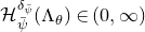 $\mathcal H_{\bar \psi}^{\delta_{\bar \psi}}(\Lambda_{\theta}) \in (0, \infty)$
, which implies that
$\mathcal H_{\bar \psi}^{\delta_{\bar \psi}}(\Lambda_{\theta}) \in (0, \infty)$
, which implies that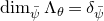 $\dim_{\bar \psi} \Lambda_{\theta} = \delta_{\bar \psi}$
. This shows the claim.
$\dim_{\bar \psi} \Lambda_{\theta} = \delta_{\bar \psi}$
. This shows the claim.
For $\psi$
non-symmetric,
$\psi$
non-symmetric, $\dim_{\psi} \Lambda_{\theta}$
is not in general equal to
$\dim_{\psi} \Lambda_{\theta}$
is not in general equal to $\delta_\psi$
.
$\delta_\psi$
.
Proposition 9.10.
For $\psi \in \mathfrak a_{\theta}^*$
positive on
$\psi \in \mathfrak a_{\theta}^*$
positive on $\mathcal L - \{0\}$
, we have
$\mathcal L - \{0\}$
, we have
 $$\delta_{\bar \psi} \le \delta_{\psi}.$$
If $\Gamma$
is Zariski dense, then the equality holds if and only if
$\Gamma$
is Zariski dense, then the equality holds if and only if $\psi = \psi \circ {\rm i}$
.
$\psi = \psi \circ {\rm i}$
.
Proof. As before, we may assume that $\theta = {\rm i}(\theta)$
. Suppose that
$\theta = {\rm i}(\theta)$
. Suppose that $\psi \neq \psi \circ {\rm i}$
. Note that
$\psi \neq \psi \circ {\rm i}$
. Note that $\delta_{\psi}=\delta_{\psi \circ {\rm i}}$
and hence both
$\delta_{\psi}=\delta_{\psi \circ {\rm i}}$
and hence both $\delta_{\psi}\psi$
and
$\delta_{\psi}\psi$
and $ \delta_{\psi} (\psi\circ {\rm i})$
are tangent to the
$ \delta_{\psi} (\psi\circ {\rm i})$
are tangent to the $\theta$
-growth indicator
$\theta$
-growth indicator $\psi_{\Gamma}^{\theta}$
(see [Reference Kim, Minsky and OhKMO24, Theorem 2.5] and [Reference Kim, Oh and WangKOW25b, Lemma 4.5]). We then have
$\psi_{\Gamma}^{\theta}$
(see [Reference Kim, Minsky and OhKMO24, Theorem 2.5] and [Reference Kim, Oh and WangKOW25b, Lemma 4.5]). We then have $\psi_\Gamma^\theta \le \delta_{\psi}\psi$
and
$\psi_\Gamma^\theta \le \delta_{\psi}\psi$
and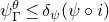 $\psi_{\Gamma}^{\theta} \le\delta_{\psi} (\psi\circ {\rm i}) $
. Hence,
$\psi_{\Gamma}^{\theta} \le\delta_{\psi} (\psi\circ {\rm i}) $
. Hence, $\psi_\Gamma^\theta \le \delta_{\psi} \bar\psi$
. Since
$\psi_\Gamma^\theta \le \delta_{\psi} \bar\psi$
. Since $\delta_{\bar\psi}\bar\psi$
is tangent to
$\delta_{\bar\psi}\bar\psi$
is tangent to $\psi_\Gamma^\theta$
, it follows that
$\psi_\Gamma^\theta$
, it follows that $\delta_{\bar \psi}\le \delta_{\psi} $
.
$\delta_{\bar \psi}\le \delta_{\psi} $
.
Now suppose that $\Gamma$
is Zariski dense and that
$\Gamma$
is Zariski dense and that $\psi\ne \psi\circ {\rm i}$
. By Theorem 3.3, there exists a unique unit vector
$\psi\ne \psi\circ {\rm i}$
. By Theorem 3.3, there exists a unique unit vector $u=u_{\delta_\psi \psi} \in \operatorname{{\rm int}} \mathcal L_\theta$
such that
$u=u_{\delta_\psi \psi} \in \operatorname{{\rm int}} \mathcal L_\theta$
such that $\psi_\Gamma^{\theta}(u)= \delta_\psi \psi(u)$
. Since
$\psi_\Gamma^{\theta}(u)= \delta_\psi \psi(u)$
. Since $\psi_\Gamma^\theta$
is i-invariant, it implies that
$\psi_\Gamma^\theta$
is i-invariant, it implies that $\psi_\Gamma^{\theta}({\rm i}(u))= \delta_\psi (\psi \circ {\rm i}) ({\rm i} (u))$
. On the other hand,
$\psi_\Gamma^{\theta}({\rm i}(u))= \delta_\psi (\psi \circ {\rm i}) ({\rm i} (u))$
. On the other hand, $u \neq {\rm i}(u)$
by Theorem 3.3. Hence the inequality
$u \neq {\rm i}(u)$
by Theorem 3.3. Hence the inequality $\psi_{\Gamma}^{\theta} \le \delta_{\psi} \psi$
and
$\psi_{\Gamma}^{\theta} \le \delta_{\psi} \psi$
and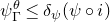 $\psi_{\Gamma}^{\theta} \le \delta_{\psi} ( \psi \circ {\rm i})$
cannot become equalities simultaneously at the same vector. This implies that
$\psi_{\Gamma}^{\theta} \le \delta_{\psi} ( \psi \circ {\rm i})$
cannot become equalities simultaneously at the same vector. This implies that $\psi_{\Gamma}^{\theta} \lt \delta_{\psi} \bar{\psi}$
and hence
$\psi_{\Gamma}^{\theta} \lt \delta_{\psi} \bar{\psi}$
and hence $\delta_{\bar{\psi}} \lt \delta_{\psi}$
.
$\delta_{\bar{\psi}} \lt \delta_{\psi}$
.
By Corollary 9.9 and Proposition 9.10, we obtain the following.
Corollary 9.11.
Let $\Gamma$
be Zariski dense in G. For any
$\Gamma$
be Zariski dense in G. For any $\psi\in \mathscr T_\Gamma$
, we have
$\psi\in \mathscr T_\Gamma$
, we have $\dim_\psi \Lambda_\theta\le 1$
and the equality holds if and only if
$\dim_\psi \Lambda_\theta\le 1$
and the equality holds if and only if $\psi$
is symmetric.
$\psi$
is symmetric.
We now prove the Ahlfors regularity of $(\Lambda_\theta, d_\psi)$
for general
$(\Lambda_\theta, d_\psi)$
for general $\psi \in \mathscr T_{\Gamma}$
.
$\psi \in \mathscr T_{\Gamma}$
.
Theorem 9.12.
Let $\Gamma$
be a
$\Gamma$
be a $\theta$
-Anosov subgroup. For any
$\theta$
-Anosov subgroup. For any $\psi\in \mathscr T_\Gamma$
, the premetric space
$\psi\in \mathscr T_\Gamma$
, the premetric space $(\Lambda_\theta, d_\psi)$
is Ahlfors s-regular for some
$(\Lambda_\theta, d_\psi)$
is Ahlfors s-regular for some $0 \lt s \le 1$
. Moreover, if
$0 \lt s \le 1$
. Moreover, if $\Gamma$
is Zariski dense, we have
$\Gamma$
is Zariski dense, we have $s = 1$
if and only if
$s = 1$
if and only if $\psi$
is symmetric.
$\psi$
is symmetric.
Proof. Let $\psi \in \mathscr T_{\Gamma}$
. By Proposition 5.5, the identity map
$\psi \in \mathscr T_{\Gamma}$
. By Proposition 5.5, the identity map $(\Lambda_{\theta}, d_{\psi}) \to (\Lambda_{\theta}, d_{\bar \psi})$
is bi-Lipschitz. Noting that
$(\Lambda_{\theta}, d_{\psi}) \to (\Lambda_{\theta}, d_{\bar \psi})$
is bi-Lipschitz. Noting that $\delta_{\bar \psi} \bar \psi \in \mathscr T_{\Gamma}$
by Lemma 3.6, we denote by
$\delta_{\bar \psi} \bar \psi \in \mathscr T_{\Gamma}$
by Lemma 3.6, we denote by $\nu := \nu_{\delta_{\bar \psi} \bar \psi}$
the
$\nu := \nu_{\delta_{\bar \psi} \bar \psi}$
the $(\Gamma, \delta_{\bar \psi}\bar \psi)$
-Patterson–Sullivan measure on
$(\Gamma, \delta_{\bar \psi}\bar \psi)$
-Patterson–Sullivan measure on $\Lambda_{\theta}$
. By Theorem 8.2, for any
$\Lambda_{\theta}$
. By Theorem 8.2, for any $\xi \in \Lambda_{\theta}$
and
$\xi \in \Lambda_{\theta}$
and $r \in [0, \operatorname{{\rm diam}}_{\bar \psi} \Lambda_{\theta})$
, we have
$r \in [0, \operatorname{{\rm diam}}_{\bar \psi} \Lambda_{\theta})$
, we have
 \begin{align} c^{-1} r \le \nu (B_{\delta_{\bar{\psi}} \bar{\psi}} (\xi, r)) \le c r,\end{align}
for some constant $c\ge 1$
depending only on
$c\ge 1$
depending only on $\psi$
. Since
$\psi$
. Since $B_{\delta_{\bar \psi} \bar \psi}(\xi, r^{\delta_{\bar \psi}}) = B_{\bar \psi}(\xi, r)$
and the identity map
$B_{\delta_{\bar \psi} \bar \psi}(\xi, r^{\delta_{\bar \psi}}) = B_{\bar \psi}(\xi, r)$
and the identity map $(\Lambda_{\theta}, d_{\psi}) \to (\Lambda_{\theta}, d_{\bar \psi})$
is bi-Lipschitz by Proposition 5.5, (9.5) implies that for some
$(\Lambda_{\theta}, d_{\psi}) \to (\Lambda_{\theta}, d_{\bar \psi})$
is bi-Lipschitz by Proposition 5.5, (9.5) implies that for some $C \ge 1$
depending only on
$C \ge 1$
depending only on $\psi$
, we have
$\psi$
, we have
 $$C^{-1} r^{\delta_{\bar \psi}} \le \nu(B_{\psi}(\xi, r)) \le C r^{\delta_{\bar \psi}}.$$
Recall $\delta_{\psi} = 1$
for
$\delta_{\psi} = 1$
for $\psi \in \mathscr T_{\Gamma}$
(Lemma 3.6). Hence
$\psi \in \mathscr T_{\Gamma}$
(Lemma 3.6). Hence $\delta_{\bar\psi}\lt 1$
for
$\delta_{\bar\psi}\lt 1$
for $\psi$
non-symmetric and
$\psi$
non-symmetric and $\Gamma$
Zariski dense by Proposition 9.10. This finishes the proof.
$\Gamma$
Zariski dense by Proposition 9.10. This finishes the proof.
9.4 Analyticity of Hausdorff dimensions
For a hyperbolic group $\Sigma$
, a representation
$\Sigma$
, a representation $\sigma : \Sigma \to G$
is called
$\sigma : \Sigma \to G$
is called $\theta$
-Anosov if
$\theta$
-Anosov if $\sigma$
has a finite kernel and its image
$\sigma$
has a finite kernel and its image $\sigma(\Sigma)$
is a
$\sigma(\Sigma)$
is a $\theta$
-Anosov subgroup of G. For a given
$\theta$
-Anosov subgroup of G. For a given $\psi \in \mathfrak a_{\theta}^*$
that is non-negative on
$\psi \in \mathfrak a_{\theta}^*$
that is non-negative on $\mathfrak a_{\theta}^+$
, the
$\mathfrak a_{\theta}^+$
, the $\psi$
-critical exponents
$\psi$
-critical exponents $\delta_{\psi}(\sigma(\Sigma))$
vary analytically on analytic families of
$\delta_{\psi}(\sigma(\Sigma))$
vary analytically on analytic families of $\theta$
-Anosov representations
$\theta$
-Anosov representations $\sigma$
in the variety
$\sigma$
in the variety $\operatorname{Hom}(\Sigma, G)$
by Bridgeman, Canary, Labourie, and Sambarino [Reference Bridgeman, Canary, Labourie and SambarinoBCL+15, Proposition 8.1] (see also [Reference Chow and SarkarCS23, § 4.4]). Hence the following is an immediate consequence of Corollary 9.9.
$\operatorname{Hom}(\Sigma, G)$
by Bridgeman, Canary, Labourie, and Sambarino [Reference Bridgeman, Canary, Labourie and SambarinoBCL+15, Proposition 8.1] (see also [Reference Chow and SarkarCS23, § 4.4]). Hence the following is an immediate consequence of Corollary 9.9.
Corollary 9.13.
Let $\Sigma$
be a non-elementary
Footnote 9
hyperbolic group and let
$\Sigma$
be a non-elementary
Footnote 9
hyperbolic group and let $\psi \in \mathfrak a_{\theta}^*$
be non-negative on
$\psi \in \mathfrak a_{\theta}^*$
be non-negative on $\mathfrak a_{\theta}^+$
. Let
$\mathfrak a_{\theta}^+$
. Let $\mathcal D \subset \operatorname{Hom}(\Sigma, G)$
be an analytic family of
$\mathcal D \subset \operatorname{Hom}(\Sigma, G)$
be an analytic family of $\theta$
-Anosov representations. Then
$\theta$
-Anosov representations. Then
 $$\sigma \mapsto \dim_{\psi} \Lambda_{\theta}(\sigma (\Sigma))$$
is analytic on $ \mathcal D$
.
$ \mathcal D$
.
9.5 (p,q)-Hausdorff dimensions
Let $\Sigma$
be a non-elementary convex cocompact subgroup of
$\Sigma$
be a non-elementary convex cocompact subgroup of $\operatorname{{\rm SO}}^\circ(n, 1)= \operatorname{{\rm Isom}}^+(\mathbb H^n)$
,
$\operatorname{{\rm SO}}^\circ(n, 1)= \operatorname{{\rm Isom}}^+(\mathbb H^n)$
, $n\ge 2$
. Let
$n\ge 2$
. Let $\operatorname{{\rm CC}}(\Sigma) $
denote the space
$\operatorname{{\rm CC}}(\Sigma) $
denote the space
 $$ \{\sigma : \Sigma \to \operatorname{{\rm SO}}^\circ(n, 1) : \text{convex cocompact, faithful representation}\}/\sim,$$
where the equivalence relation is given by conjugations. As in the introduction, for $\sigma \in \operatorname{{\rm CC}}(\Sigma)$
, we denote by
$\sigma \in \operatorname{{\rm CC}}(\Sigma)$
, we denote by $\Lambda_{\sigma} \subset \mathbb S^{n-1} \times \mathbb S^{n-1}$
the limit set of the self-joining subgroup
$\Lambda_{\sigma} \subset \mathbb S^{n-1} \times \mathbb S^{n-1}$
the limit set of the self-joining subgroup $\Sigma_{\sigma} := (\operatorname{{\rm id}} \times \sigma)(\Sigma) \lt \operatorname{{\rm SO}}^\circ(n, 1) \times \operatorname{{\rm SO}}^\circ(n, 1)$
, which is well-defined up to translations. The Hausdorff dimension of
$\Sigma_{\sigma} := (\operatorname{{\rm id}} \times \sigma)(\Sigma) \lt \operatorname{{\rm SO}}^\circ(n, 1) \times \operatorname{{\rm SO}}^\circ(n, 1)$
, which is well-defined up to translations. The Hausdorff dimension of $\Lambda_{\sigma}$
with respect to a Riemannian metric on
$\Lambda_{\sigma}$
with respect to a Riemannian metric on $\mathbb S^{n-1}\times \mathbb S^{n-1}$
is equal to
$\mathbb S^{n-1}\times \mathbb S^{n-1}$
is equal to $\max (\dim \Lambda_\Sigma, \dim \Lambda_{\sigma(\Sigma)} )$
, where
$\max (\dim \Lambda_\Sigma, \dim \Lambda_{\sigma(\Sigma)} )$
, where $\Lambda_{\Sigma} \subset \mathbb S^{n-1}$
and
$\Lambda_{\Sigma} \subset \mathbb S^{n-1}$
and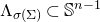 $\Lambda_{\sigma(\Sigma)}\subset \mathbb S^{n-1}$
are limit sets of
$\Lambda_{\sigma(\Sigma)}\subset \mathbb S^{n-1}$
are limit sets of $\Sigma$
and
$\Sigma$
and $\sigma(\Sigma)$
, respectively, and Hausdorff dimensions are computed with respect to a Riemannian metric on
$\sigma(\Sigma)$
, respectively, and Hausdorff dimensions are computed with respect to a Riemannian metric on $\mathbb S^{n-1}$
(see [Reference Kim, Minsky and OhKMO23, Theorem 1.1]).
$\mathbb S^{n-1}$
(see [Reference Kim, Minsky and OhKMO23, Theorem 1.1]).
For a pair (p, q) of positive real numbers, let $d_{p, q}$
be the premetric on
$d_{p, q}$
be the premetric on $\mathbb S^{n-1} \times \mathbb S^{n-1}$
defined as
$\mathbb S^{n-1} \times \mathbb S^{n-1}$
defined as
 $$d_{p, q}(\xi, \eta) = d_{\mathbb S^{n-1}} (\xi_1, \eta_1)^p d_{\mathbb S^{n-1}}(\xi_2, \eta_2)^q,$$
where $\xi = (\xi_1, \xi_2), \eta = (\eta_1, \eta_2) \in \mathbb S^{n-1} \times \mathbb S^{n-1}$
and
$\xi = (\xi_1, \xi_2), \eta = (\eta_1, \eta_2) \in \mathbb S^{n-1} \times \mathbb S^{n-1}$
and $d_{\mathbb S^{n-1}}$
is a Riemannian metric on
$d_{\mathbb S^{n-1}}$
is a Riemannian metric on $\mathbb S^{n-1}$
. We also denote by
$\mathbb S^{n-1}$
. We also denote by $\dim_{p, q}$
the Hausdorff dimension with respect to
$\dim_{p, q}$
the Hausdorff dimension with respect to $d_{p, q}$
. Let
$d_{p, q}$
. Let $\delta_{p,q}(\sigma)$
denote the critical exponent of the series
$\delta_{p,q}(\sigma)$
denote the critical exponent of the series
 $$s\mapsto \sum_{\gamma \in \Sigma} e ^{- s(pd_{\mathbb H^n}(o, \gamma o) + q d_{\mathbb H^n}(o, \sigma(\gamma) o))}.$$
We deduce the following.
Corollary 9.14.
Let $\Sigma$
be a non-elementary convex cocompact subgroup of
$\Sigma$
be a non-elementary convex cocompact subgroup of $\operatorname{{\rm SO}}^\circ(n, 1)$
,
$\operatorname{{\rm SO}}^\circ(n, 1)$
, $n\ge 2$
. Let p,q be positive real numbers.
$n\ge 2$
. Let p,q be positive real numbers.
-
(1) For any
$\sigma \in \operatorname{{\rm CC}}(\Sigma)$
, we have
$$\dim_{p, q}\Lambda_{\sigma} =\delta_{p,q}(\sigma).$$
-
(2) For any
$\sigma \in \operatorname{{\rm CC}}(\Sigma)$
, we have and the equality holds if and only if
$$\dim_{p, q} \Lambda_{\sigma} \le \left( \frac{p}{\dim \Lambda_{\Sigma}} + \frac{q}{\dim \Lambda_{\sigma(\Sigma)}} \right)^{-1}$$
$\rho = \operatorname{{\rm id}}$
.
-
(3) Moreover, the map
is an analytic function on any analytic subfamily of
$$\sigma \mapsto\dim_{p, q}\Lambda_{\sigma} $$
$\operatorname{{\rm CC}}(\Sigma)$
. In particular, for
$n=2,3$
, it is analytic on
$\operatorname{{\rm CC}}(\Sigma)$
.


Proof. Identifying the Cartan subspace $\mathfrak a$
of
$\mathfrak a$
of $\operatorname{{\rm SO}}^\circ(n, 1) \times \operatorname{{\rm SO}}^\circ(n, 1)$
with
$\operatorname{{\rm SO}}^\circ(n, 1) \times \operatorname{{\rm SO}}^\circ(n, 1)$
with $\mathbb R^2$
and
$\mathbb R^2$
and $\mathfrak a^+$
with
$\mathfrak a^+$
with $\mathbb R_{\ge 0}^2$
, consider the linear form
$\mathbb R_{\ge 0}^2$
, consider the linear form $\Psi\in \mathfrak a^*$
defined by
$\Psi\in \mathfrak a^*$
defined by $\Psi(u_1, u_2)= pu_1+ q u_2$
. Since
$\Psi(u_1, u_2)= pu_1+ q u_2$
. Since $d_{\mathbb S^{n-1}}(\xi, \eta)=e^{-\mathcal G(\xi, \eta)}$
is a
$d_{\mathbb S^{n-1}}(\xi, \eta)=e^{-\mathcal G(\xi, \eta)}$
is a $\operatorname{{\rm SO}}(n)$
-invariant metric and hence a Riemannian metric, where
$\operatorname{{\rm SO}}(n)$
-invariant metric and hence a Riemannian metric, where $\mathcal G$
is the Gromov product on
$\mathcal G$
is the Gromov product on $\mathbb S^{n-1}\simeq\partial \mathbb H^n$
, we have
$\mathbb S^{n-1}\simeq\partial \mathbb H^n$
, we have $d_{\Psi} = d_{p, q}$
, where
$d_{\Psi} = d_{p, q}$
, where $d_{\Psi}$
is defined in (5.1). Since the opposition involution i is trivial for
$d_{\Psi}$
is defined in (5.1). Since the opposition involution i is trivial for $\operatorname{{\rm SO}}^\circ(n, 1) \times \operatorname{{\rm SO}}^\circ(n, 1)$
, the linear form
$\operatorname{{\rm SO}}^\circ(n, 1) \times \operatorname{{\rm SO}}^\circ(n, 1)$
, the linear form $\Psi$
is symmetric and hence claims (1) and (3) follow from Corollaries 9.9 and 9.13, respectively, applied to any analytic subfamily of
$\Psi$
is symmetric and hence claims (1) and (3) follow from Corollaries 9.9 and 9.13, respectively, applied to any analytic subfamily of $ \{(\operatorname{{\rm id}}\times \sigma):\Sigma \to \operatorname{{\rm SO}}^\circ(n, 1) \times \operatorname{{\rm SO}}^\circ(n, 1) : \sigma \in \operatorname{{\rm CC}}(\Sigma)\}$
. For
$ \{(\operatorname{{\rm id}}\times \sigma):\Sigma \to \operatorname{{\rm SO}}^\circ(n, 1) \times \operatorname{{\rm SO}}^\circ(n, 1) : \sigma \in \operatorname{{\rm CC}}(\Sigma)\}$
. For $n=2,3$
,
$n=2,3$
, $\operatorname{{\rm CC}}(\Sigma)$
is known to be analytic (cf. [Reference BersBer70], [Reference MardenMar74, Theorem 10.8], and [Reference Imayoshi and TaniguchiIT92]). Hence, the last part of claim (3) follows. Claim (2) follows from claim (1) and the following Theorem 9.15.
$\operatorname{{\rm CC}}(\Sigma)$
is known to be analytic (cf. [Reference BersBer70], [Reference MardenMar74, Theorem 10.8], and [Reference Imayoshi and TaniguchiIT92]). Hence, the last part of claim (3) follows. Claim (2) follows from claim (1) and the following Theorem 9.15.
The following theorem is due to Bishop and Steger [Reference Bishop and StegerBS93, Theorem 2] for $n=2$
and to Burger [Reference BurgerBur93, Theorem 1(a)] in general. We denote by
$n=2$
and to Burger [Reference BurgerBur93, Theorem 1(a)] in general. We denote by $\delta_{\Sigma}$
the critical exponent of
$\delta_{\Sigma}$
the critical exponent of $\Sigma$
, the abscissa of convergence of the Poincaré series
$\Sigma$
, the abscissa of convergence of the Poincaré series $s \mapsto \sum_{\gamma \in \Sigma} e^{-s d_{\mathbb H^n}(o, \gamma o)}$
.
$s \mapsto \sum_{\gamma \in \Sigma} e^{-s d_{\mathbb H^n}(o, \gamma o)}$
.
Theorem 9.15.
For each $\sigma \in \operatorname{{\rm CC}}(\Sigma)$
, we have
$\sigma \in \operatorname{{\rm CC}}(\Sigma)$
, we have
 $$\delta_{p, q}(\sigma) \le \bigg(\frac{p}{\delta_{\Sigma}} + \frac{q}{\delta_{\sigma(\Sigma)}} \bigg)^{\!\!-1}$$
and the equality holds if and only if $\sigma = \operatorname{{\rm id}}$
.
$\sigma = \operatorname{{\rm id}}$
.
Proof. We explain how to deduce this from [Reference BurgerBur93, Theorem 1(a)]. We again identify the Cartan subspace $\mathfrak a$
of
$\mathfrak a$
of $\operatorname{{\rm SO}}^\circ(n, 1) \times \operatorname{{\rm SO}}^\circ(n, 1)$
with
$\operatorname{{\rm SO}}^\circ(n, 1) \times \operatorname{{\rm SO}}^\circ(n, 1)$
with $\mathbb R^2$
. For each
$\mathbb R^2$
. For each $i=1,2$
, denote by
$i=1,2$
, denote by $\delta_i$
the
$\delta_i$
the $\alpha_i$
-critical exponent of
$\alpha_i$
-critical exponent of $\Sigma_{\sigma} = (\operatorname{{\rm id}} \times \sigma)(\Sigma),$
where
$\Sigma_{\sigma} = (\operatorname{{\rm id}} \times \sigma)(\Sigma),$
where $\alpha_i : \mathfrak a \to \mathbb R$
,
$\alpha_i : \mathfrak a \to \mathbb R$
, $(u_1, u_2) \mapsto u_i$
. Then,
$(u_1, u_2) \mapsto u_i$
. Then, $\delta_1=\delta_\Sigma$
and
$\delta_1=\delta_\Sigma$
and $\delta_{2} = \delta_{\sigma(\Sigma)}$
. If we set
$\delta_{2} = \delta_{\sigma(\Sigma)}$
. If we set $\alpha_i':= \delta_i \alpha_i$
, then
$\alpha_i':= \delta_i \alpha_i$
, then $\delta_{\alpha_i'}=1$
for each
$\delta_{\alpha_i'}=1$
for each $i=1,2$
and hence Burger’s theorem [Reference BurgerBur93, Theorem 1(a)] implies that the critical exponent of any convex combination of
$i=1,2$
and hence Burger’s theorem [Reference BurgerBur93, Theorem 1(a)] implies that the critical exponent of any convex combination of $\alpha_1'$
and
$\alpha_1'$
and $\alpha_2'$
is at most one and is equal to one only when
$\alpha_2'$
is at most one and is equal to one only when $\sigma=\operatorname{{\rm id}}$
.
$\sigma=\operatorname{{\rm id}}$
.
Since
 $$ p\alpha_1+q\alpha_2 = \left(\frac{p}{\delta_{1}} + \frac{q}{\delta_{2}} \right) \frac{({p}/{\delta_{1}}) \alpha_1' + ({q}/{\delta_{2}}) \alpha_2'}{({p}/{\delta_{1}}) + ({q}/{\delta_{2}})} =\left(\frac{p}{\delta_{1}} + \frac{q}{\delta_{2}} \right) \Psi_0, $$
where $\Psi_0 := ({({p}/{\delta_{1}}) \alpha_1' + ({q}/{\delta_{2}}) \alpha_2'})/({{p}/{\delta_{1}} + {q}/{\delta_{2}}})$
is a convex combination of
$\Psi_0 := ({({p}/{\delta_{1}}) \alpha_1' + ({q}/{\delta_{2}}) \alpha_2'})/({{p}/{\delta_{1}} + {q}/{\delta_{2}}})$
is a convex combination of $\alpha_1'$
and
$\alpha_1'$
and $ \alpha_2'$
, we obtain
$ \alpha_2'$
, we obtain
 \begin{equation} \delta_{p,q}(\sigma) = \delta_{p\alpha_1+q\alpha_2}=\left( \frac{p}{\delta_{1}} + \frac{q}{\delta_{2}} \right)^{-1} \delta_{\Psi_0} \le \left( \frac{p}{\delta_{1}} + \frac{q}{\delta_{2}} \right)^{-1} \end{equation}
and the equality holds if and only if $\sigma = \operatorname{{\rm id}}$
.
$\sigma = \operatorname{{\rm id}}$
.
Remark 9.16 We remark that in Corollary 9.14, the hypothesis $p, q\gt 0$
was imposed to be able to consider all
$p, q\gt 0$
was imposed to be able to consider all $\sigma \in \operatorname{{\rm CC}}(\Sigma)$
. If we replace
$\sigma \in \operatorname{{\rm CC}}(\Sigma)$
. If we replace $\operatorname{{\rm CC}}(\Sigma)$
by a subset
$\operatorname{{\rm CC}}(\Sigma)$
by a subset $\mathcal D \subset \operatorname{{\rm CC}}(\Sigma)$
, then Corollary 9.14 holds for any
$\mathcal D \subset \operatorname{{\rm CC}}(\Sigma)$
, then Corollary 9.14 holds for any $p, q \in \mathbb R$
such that
$p, q \in \mathbb R$
such that $p u_1 + q u_2 \gt 0$
for all non-zero
$p u_1 + q u_2 \gt 0$
for all non-zero $(u_1, u_2) \in \mathcal L(\Sigma_\sigma)$
and all
$(u_1, u_2) \in \mathcal L(\Sigma_\sigma)$
and all $\sigma \in \mathcal D$
.
$\sigma \in \mathcal D$
.
10. Hausdorff dimensions with respect to Riemannian metrics
Let G be a connected semisimple real algebraic group. As before, let $\theta$
be a non-empty subset of the set
$\theta$
be a non-empty subset of the set $\Pi$
of simple roots of
$\Pi$
of simple roots of $(\mathfrak g, \mathfrak a)$
. We denote by
$(\mathfrak g, \mathfrak a)$
. We denote by
 $$\dim \Lambda_{\theta}$$
the Hausdorff dimension of $\Lambda_{\theta}$
with respect to a Riemannian distance
$\Lambda_{\theta}$
with respect to a Riemannian distance $d_{\rm Riem}$
on
$d_{\rm Riem}$
on $\mathcal F_{\theta}$
. As any two Riemannian metrics are bi-Lipschitz,
$\mathcal F_{\theta}$
. As any two Riemannian metrics are bi-Lipschitz, $\dim \Lambda_\theta$
is well-defined independent of the choice of a Riemannian metric. In this section, we present an estimate on
$\dim \Lambda_\theta$
is well-defined independent of the choice of a Riemannian metric. In this section, we present an estimate on $\dim \Lambda_\theta$
.
$\dim \Lambda_\theta$
.
10.1 Tits representations and the sum of Tits weights
Let $\mathbf G$
be the semisimple algebraic group defined over
$\mathbf G$
be the semisimple algebraic group defined over $\mathbb R$
such that
$\mathbb R$
such that $G=\mathbf G(\mathbb R)^\circ$
. There exists an exact sequence
$G=\mathbf G(\mathbb R)^\circ$
. There exists an exact sequence $\tilde{\mathbf G}\to_{\tilde p} \mathbf G\to_{\bar p} \bar{\mathbf G},$
where
$\tilde{\mathbf G}\to_{\tilde p} \mathbf G\to_{\bar p} \bar{\mathbf G},$
where $\tilde {\mathbf G}$
and
$\tilde {\mathbf G}$
and $\bar{\mathbf G}$
are, respectively, simply connected and adjoint semisimple
$\bar{\mathbf G}$
are, respectively, simply connected and adjoint semisimple $\mathbb R$
-groups and
$\mathbb R$
-groups and $\tilde p$
and
$\tilde p$
and $\bar p$
are central
$\bar p$
are central $\mathbb R$
-isogenies (see [Reference Borel and TitsBT65] and [Reference MargulisMar91, Proposition 1.4.11]).
$\mathbb R$
-isogenies (see [Reference Borel and TitsBT65] and [Reference MargulisMar91, Proposition 1.4.11]).
Recall that for $\alpha \in \Pi$
,
$\alpha \in \Pi$
, $\omega_\alpha$
denotes the (restricted) fundamental weight associated to
$\omega_\alpha$
denotes the (restricted) fundamental weight associated to $\alpha$
as defined in (2.1). The first part of the following theorem immediately follows as a special case of a theorem of Tits [Reference TitsTit71], and the second part is remarked in [Reference BenoistBen97] and proved in [Reference SmilgaSmi18].
$\alpha$
as defined in (2.1). The first part of the following theorem immediately follows as a special case of a theorem of Tits [Reference TitsTit71], and the second part is remarked in [Reference BenoistBen97] and proved in [Reference SmilgaSmi18].
Theorem 10.1 (See [Reference TitsTit71, Theorem 7.2] and [Reference SmilgaSmi18, Lemma 2.13]). For each $\alpha\in \Pi$
, there exists an irreducible
$\alpha\in \Pi$
, there exists an irreducible $\mathbb R$
-representation
$\mathbb R$
-representation ${\tilde{\rho}}_{\alpha}: \tilde{\mathbf{G}}\to \operatorname{GL} (\mathbf V_{\alpha}) $
whose highest (restricted) weight
${\tilde{\rho}}_{\alpha}: \tilde{\mathbf{G}}\to \operatorname{GL} (\mathbf V_{\alpha}) $
whose highest (restricted) weight $\chi_{\alpha}$
is equal to
$\chi_{\alpha}$
is equal to $k_\alpha \omega_\alpha$
for some positive integer
$k_\alpha \omega_\alpha$
for some positive integer $k_\alpha$
and whose highest-weight space is one-dimensional. Moreover, all weights of
$k_\alpha$
and whose highest-weight space is one-dimensional. Moreover, all weights of $\tilde\rho_{\alpha}$
are
$\tilde\rho_{\alpha}$
are $\chi_\alpha$
,
$\chi_\alpha$
, $\chi_\alpha-\alpha$
, and weights of the form
$\chi_\alpha-\alpha$
, and weights of the form $\chi_{\alpha} - \alpha - \sum_{\beta \in \Pi} n_{\beta} \beta$
with
$\chi_{\alpha} - \alpha - \sum_{\beta \in \Pi} n_{\beta} \beta$
with $n_\beta$
non-negative integers.
$n_\beta$
non-negative integers.
For each $\alpha\in \Pi$
, we fix once and for all a representation
$\alpha\in \Pi$
, we fix once and for all a representation $\tilde\rho_\alpha:\tilde{\mathbf{G}}\to \operatorname{GL} (\mathbf V_\alpha)$
as in Theorem 10.1 with minimal
$\tilde\rho_\alpha:\tilde{\mathbf{G}}\to \operatorname{GL} (\mathbf V_\alpha)$
as in Theorem 10.1 with minimal $k_\alpha$
. Since
$k_\alpha$
. Since $\tilde p$
and
$\tilde p$
and $\bar p$
are central isogenies and
$\bar p$
are central isogenies and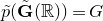 $\tilde p(\tilde{\mathbf G}(\mathbb R))=G$
, the representation
$\tilde p(\tilde{\mathbf G}(\mathbb R))=G$
, the representation $\tilde\rho_\alpha$
induces a projective representation
$\tilde\rho_\alpha$
induces a projective representation
 \begin{equation} \rho_\alpha: G\to \operatorname{{\rm PGL}}(V_\alpha),\end{equation}
where $V_\alpha=\mathbf V_\alpha(\mathbb R)$
. Since the restriction of
$V_\alpha=\mathbf V_\alpha(\mathbb R)$
. Since the restriction of $\tilde \rho_\alpha$
to
$\tilde \rho_\alpha$
to $\tilde{\mathbf G}(\mathbb R)$
and
$\tilde{\mathbf G}(\mathbb R)$
and $\rho_\alpha$
induce the same representation of the Lie algebra
$\rho_\alpha$
induce the same representation of the Lie algebra $\mathfrak g$
to
$\mathfrak g$
to $\mathfrak {gl}(V_\alpha)$
, their restricted weights are the same. We call
$\mathfrak {gl}(V_\alpha)$
, their restricted weights are the same. We call
 \begin{equation}\rho_\alpha \quad \text{and} \quad \chi_\alpha\end{equation}
the Tits representation and the Tits weight associated to $\alpha$
, respectively.
$\alpha$
, respectively.
Let $\rho$
denote the half-sum of all positive roots for
$\rho$
denote the half-sum of all positive roots for $(\mathfrak g, \mathfrak a)$
counted with multiplicity:
$(\mathfrak g, \mathfrak a)$
counted with multiplicity: $2\rho =\sum_{\alpha\in \Phi^+} (\dim \mathfrak g^{\alpha} ) \alpha$
. In terms of the restricted fundamental weights
$2\rho =\sum_{\alpha\in \Phi^+} (\dim \mathfrak g^{\alpha} ) \alpha$
. In terms of the restricted fundamental weights $\omega_\alpha$
, we then have
$\omega_\alpha$
, we then have
 \begin{equation} \rho=\sum_{\alpha\in \Pi} c_\alpha \omega_\alpha,\end{equation}
where $c_\alpha = \dim \mathfrak g^{\alpha}$
if
$c_\alpha = \dim \mathfrak g^{\alpha}$
if $2\alpha$
is not a root, and
$2\alpha$
is not a root, and $c_\alpha = ({1}/{2})(\dim \mathfrak g^{\alpha} + 2 \dim \mathfrak g^{2 \alpha}) $
otherwise (cf. [Reference BourbakiBou02]). If G is split over
$c_\alpha = ({1}/{2})(\dim \mathfrak g^{\alpha} + 2 \dim \mathfrak g^{2 \alpha}) $
otherwise (cf. [Reference BourbakiBou02]). If G is split over $\mathbb R$
, we have
$\mathbb R$
, we have $\chi_\alpha=\omega_\alpha$
for all
$\chi_\alpha=\omega_\alpha$
for all $\alpha\in \Pi$
and hence
$\alpha\in \Pi$
and hence $ \sum_{\alpha \in \Pi} \chi_{\alpha}=\rho$
. In general, we do not have this identity, which motivates the following definition.
$ \sum_{\alpha \in \Pi} \chi_{\alpha}=\rho$
. In general, we do not have this identity, which motivates the following definition.
Definition 10.2.
Define ${\mathsf c}_\theta$
to be the minimum number
${\mathsf c}_\theta$
to be the minimum number $c\ge 0$
such that
$c\ge 0$
such that
 $$\sum_{\alpha\in \theta} (\chi_\alpha + \chi_{{\rm i}(\alpha)}) \le c\cdot \rho \quad \text{on } \mathfrak a^+.$$
We also set $\mathsf{c}_G := \mathsf{c}_{\Pi}$
.
$\mathsf{c}_G := \mathsf{c}_{\Pi}$
.
It is easy to check that $0\lt \mathsf{c}_{\theta} \le \mathsf{c}_G$
, and, moreover, if
$0\lt \mathsf{c}_{\theta} \le \mathsf{c}_G$
, and, moreover, if $\theta \cap {\rm i}(\theta) = \emptyset$
, then
$\theta \cap {\rm i}(\theta) = \emptyset$
, then $\mathsf{c}_{\theta} \le {\mathsf{c}_G}/{2}$
. By our choice of the Tits representation of G, note that
$\mathsf{c}_{\theta} \le {\mathsf{c}_G}/{2}$
. By our choice of the Tits representation of G, note that ${\mathsf c}_G$
depends only on the Lie algebra
${\mathsf c}_G$
depends only on the Lie algebra $\mathfrak g$
; hence, we sometimes write
$\mathfrak g$
; hence, we sometimes write ${\mathsf c}_G=\mathsf{c}_{\mathfrak g}$
. The proof of the following lemma was provided by I. Smilga.
${\mathsf c}_G=\mathsf{c}_{\mathfrak g}$
. The proof of the following lemma was provided by I. Smilga.
Lemma 10.3.
We have $\sum_{\alpha\in \Pi} \chi_\alpha \le \rho,$
and hence
$\sum_{\alpha\in \Pi} \chi_\alpha \le \rho,$
and hence
 $$\mathsf c_{\mathfrak g}\le 2.$$
Proof. Let $\mathfrak g_\mathbb C$
be the complexification of
$\mathfrak g_\mathbb C$
be the complexification of $\mathfrak g=\operatorname{Lie}G$
and
$\mathfrak g=\operatorname{Lie}G$
and $\mathfrak {h}$
be a Cartan subalgebra of
$\mathfrak {h}$
be a Cartan subalgebra of $\mathfrak g_\mathbb C$
containing
$\mathfrak g_\mathbb C$
containing $\mathfrak a$
. Since
$\mathfrak a$
. Since $\mathfrak a\subset \mathfrak {h}$
, we have a natural restriction map
$\mathfrak a\subset \mathfrak {h}$
, we have a natural restriction map $\pi : \mathfrak {h}^* \to \mathfrak a^*$
. Recall the restricted fundamental weights
$\pi : \mathfrak {h}^* \to \mathfrak a^*$
. Recall the restricted fundamental weights $\omega_1, \ldots, \omega_s$
defined in (2.1), where
$\omega_1, \ldots, \omega_s$
defined in (2.1), where $s=\dim \mathfrak a $
; they form a basis of
$s=\dim \mathfrak a $
; they form a basis of $\mathfrak a^*$
. We denote by
$\mathfrak a^*$
. We denote by $\bar \omega_1, \ldots, \bar \omega_r$
the fundamental weights of
$\bar \omega_1, \ldots, \bar \omega_r$
the fundamental weights of $(\mathfrak g_{\mathbb C}, \mathfrak {h})$
, where
$(\mathfrak g_{\mathbb C}, \mathfrak {h})$
, where $r=\dim \mathfrak {h}$
, which have been chosen compatibly with
$r=\dim \mathfrak {h}$
, which have been chosen compatibly with $\omega_j$
values so that
$\omega_j$
values so that $\pi$
sends each
$\pi$
sends each $\bar \omega_j$
to some linear combination
$\bar \omega_j$
to some linear combination $\sum_{i} c_{j, i} \omega_i$
, where the
$\sum_{i} c_{j, i} \omega_i$
, where the $c_{j, i}$
are non-negative integers. They form a basis of
$c_{j, i}$
are non-negative integers. They form a basis of $\mathfrak {h}^*$
.
$\mathfrak {h}^*$
.
Set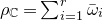 $\rho_\mathbb C=\sum_{i=1}^r \bar \omega_i$
, which is equal to the half-sum of all positive roots of
$\rho_\mathbb C=\sum_{i=1}^r \bar \omega_i$
, which is equal to the half-sum of all positive roots of $(\mathfrak g_\mathbb C, \mathfrak {h})$
. Then,
$(\mathfrak g_\mathbb C, \mathfrak {h})$
. Then,
 $$\rho=\pi( \rho_{\mathbb C})= \sum_i d_i \omega_i,$$
where $d_i=\sum_j c_{j, i}\in \mathbb N$
. For the Tits weights
$d_i=\sum_j c_{j, i}\in \mathbb N$
. For the Tits weights $\chi_i=\kappa_i \omega_i$
for
$\chi_i=\kappa_i \omega_i$
for $i=1,\ldots ,s$
, recall that
$i=1,\ldots ,s$
, recall that $\kappa_i$
is the smallest positive integer
$\kappa_i$
is the smallest positive integer $\kappa$
such that
$\kappa$
such that $\kappa \omega_i$
is proximal; that is, its highest-weight space is one-dimensional. In view of the Killing form, we may consider
$\kappa \omega_i$
is proximal; that is, its highest-weight space is one-dimensional. In view of the Killing form, we may consider $\mathfrak a^*$
as a subset of
$\mathfrak a^*$
as a subset of $\mathfrak {h}^*$
. We have the following facts:
$\mathfrak {h}^*$
. We have the following facts:
-
– a representation with the highest weight
$\chi\in \mathfrak {h}^*$
is proximal if and only if
$\chi$
actually lies in
$\mathfrak a^*$
(see [Reference Abels, Margulis and SoiferAMS95, Theorem 6.3]); and -
– each coefficient
$\kappa_i$
is either 1 or 2 (see [Reference BenoistBen00, § 2.3]).


We now claim that $\kappa_i\le d_i$
for all
$\kappa_i\le d_i$
for all $1\le i\le s$
; this implies that
$1\le i\le s$
; this implies that $\sum_{i} \chi_i=\sum_i \kappa_i \omega_i\le \rho$
. This is clear if
$\sum_{i} \chi_i=\sum_i \kappa_i \omega_i\le \rho$
. This is clear if $\kappa_i=1$
, since
$\kappa_i=1$
, since $d_i\ge 1$
. Thus, suppose that
$d_i\ge 1$
. Thus, suppose that $\kappa_i=2$
and let us show that
$\kappa_i=2$
and let us show that $d_i\ge 2$
. Then,
$d_i\ge 2$
. Then, $\chi_i=2 \omega_i$
lies in
$\chi_i=2 \omega_i$
lies in $\mathfrak a^*$
and is an integral weight; hence it is equal to some linear combination
$\mathfrak a^*$
and is an integral weight; hence it is equal to some linear combination $\sum_j c_j \bar \omega_j$
with non-negative integer coefficients
$\sum_j c_j \bar \omega_j$
with non-negative integer coefficients $c_j$
. Moreover, the sum
$c_j$
. Moreover, the sum $\sum_j c_j$
cannot exceed 2, because
$\sum_j c_j$
cannot exceed 2, because $\pi$
has to map
$\pi$
has to map $\sum_j c_j \bar \omega_j$
to
$\sum_j c_j \bar \omega_j$
to $2 \omega_i$
, and it maps each
$2 \omega_i$
, and it maps each $\bar \omega_j$
to some non-zero sum of the
$\bar \omega_j$
to some non-zero sum of the $\omega_k$
. We are left with three cases:
$\omega_k$
. We are left with three cases:
-
(a)
$2 \omega_i = \bar \omega_j$
for some j; -
(b)
$2 \omega_i = \bar \omega_j + \bar \omega_{k}$
for some distinct j and k; and -
(c)
$2 \omega_i = 2 \bar \omega_j$
for some j.



We can rule out case (c), because then $\omega_i = \bar \omega_j$
would be proximal, which contradicts
$\omega_i = \bar \omega_j$
would be proximal, which contradicts $\kappa_i = 2$
. In case (a), we obtain that
$\kappa_i = 2$
. In case (a), we obtain that $c_{j, i}=2$
and hence
$c_{j, i}=2$
and hence $d_i$
is at least 2. In case (b), applying
$d_i$
is at least 2. In case (b), applying $\pi$
on both sides, we necessarily have
$\pi$
on both sides, we necessarily have $\pi(\bar \omega_j) = \pi(\bar \omega_{k}) = \omega_i$
, so
$\pi(\bar \omega_j) = \pi(\bar \omega_{k}) = \omega_i$
, so $c_{j, i} = c_{k, i} = 1$
and hence
$c_{j, i} = c_{k, i} = 1$
and hence $d_i$
is also at least 2.
$d_i$
is also at least 2.
The bound on $\mathsf c_{G}$
can be improved in certain cases. For example, for
$\mathsf c_{G}$
can be improved in certain cases. For example, for $\mathfrak g=\mathfrak {so}(n,1)$
,
$\mathfrak g=\mathfrak {so}(n,1)$
, $n\ge 2$
, we have
$n\ge 2$
, we have $\Pi=\{\alpha\}$
,
$\Pi=\{\alpha\}$
, $\rho=(({n-1})/{2}) \alpha$
and
$\rho=(({n-1})/{2}) \alpha$
and $\chi_\alpha=\omega_\alpha={\alpha}/{2}$
; hence
$\chi_\alpha=\omega_\alpha={\alpha}/{2}$
; hence $\mathsf c_{\mathfrak g}={2}/({n-1})$
.
$\mathsf c_{\mathfrak g}={2}/({n-1})$
.
10.2 Riemannian metric on
$\mathcal F_\theta$

For each $\alpha \in \Pi$
, we denote by
$\alpha \in \Pi$
, we denote by $V_{\alpha}^+$
the highest-weight space of
$V_{\alpha}^+$
the highest-weight space of $\rho_{\alpha}$
and by
$\rho_{\alpha}$
and by $V_{\alpha}^{\lt }$
its unique complementary A-invariant subspace in
$V_{\alpha}^{\lt }$
its unique complementary A-invariant subspace in $V_{\alpha}$
. Then, the map
$V_{\alpha}$
. Then, the map $g \in G \mapsto (\rho_{\alpha}(g)V_{\alpha}^+)_{\alpha \in \theta}$
factors through a proper immersion
$g \in G \mapsto (\rho_{\alpha}(g)V_{\alpha}^+)_{\alpha \in \theta}$
factors through a proper immersion
 \begin{equation} \mathcal F_{\theta} \to \prod_{\alpha \in\theta} \mathbb{P}(V_{\alpha}).\end{equation}
Let $\langle \cdot, \cdot \rangle_{\alpha}$
be a K-invariant inner product on
$\langle \cdot, \cdot \rangle_{\alpha}$
be a K-invariant inner product on $V_{\alpha}$
with respect to which A is symmetric, so that
$V_{\alpha}$
with respect to which A is symmetric, so that $V_{\alpha}^+$
is perpendicular to
$V_{\alpha}^+$
is perpendicular to $V_{\alpha}^{\lt }$
. We denote by
$V_{\alpha}^{\lt }$
. We denote by $\| \cdot \|_{\alpha}$
the norm on
$\| \cdot \|_{\alpha}$
the norm on $V_{\alpha}$
induced by
$V_{\alpha}$
induced by $\langle \cdot, \cdot \rangle_{\alpha}$
. We also use the notation
$\langle \cdot, \cdot \rangle_{\alpha}$
. We also use the notation $\| \cdot \|_{\alpha}$
for a bi-
$\| \cdot \|_{\alpha}$
for a bi- $\rho_{\alpha}(K)$
-invariant norm on
$\rho_{\alpha}(K)$
-invariant norm on $\operatorname{GL}(V_{\alpha})$
. The angle
$\operatorname{GL}(V_{\alpha})$
. The angle $\angle (E, F)$
between a line E and a subspace F is defined as the minimum of all angles between all non-zero
$\angle (E, F)$
between a line E and a subspace F is defined as the minimum of all angles between all non-zero $v\in E$
and non-zero
$v\in E$
and non-zero $w\in F$
.
$w\in F$
.
We write $g V_{\alpha}^+ := \rho_{\alpha}(g) V_{\alpha}^+$
and
$g V_{\alpha}^+ := \rho_{\alpha}(g) V_{\alpha}^+$
and $g V_{\alpha}^{\lt } := \rho_{\alpha}(g) V_{\alpha}^{\lt }$
for
$g V_{\alpha}^{\lt } := \rho_{\alpha}(g) V_{\alpha}^{\lt }$
for $g \in G$
and
$g \in G$
and $\alpha \in \Pi$
. Up to a Lipschitz equivalence, the Riemannian distance
$\alpha \in \Pi$
. Up to a Lipschitz equivalence, the Riemannian distance $d_{\rm Riem}$
on
$d_{\rm Riem}$
on $\mathcal F_\theta=G/P_\theta$
satisfies that for all
$\mathcal F_\theta=G/P_\theta$
satisfies that for all $g_1, g_2 \in G$
,
$g_1, g_2 \in G$
,
 $$d_{\rm Riem}(g_1P_{\theta}, g_2 P_{\theta}) = \sqrt{\sum_{\alpha \in \theta} \sin^2 \angle (g_1 V_{\alpha}^+, g_2 V_{\alpha}^+)}.$$
The Gromov product $\mathcal G$
on
$\mathcal G$
on $\mathcal F^{(2)}$
can be expressed in terms of angles between appropriate subspaces as follows.
$\mathcal F^{(2)}$
can be expressed in terms of angles between appropriate subspaces as follows.
Lemma 10.4 (See [Reference QuintQui02b, Lemma 6.4] and [Reference Lee and OhLO23, Lemma 3.11]). For $(\xi, \eta) \in \mathcal F^{(2)}$
, we have that for any
$(\xi, \eta) \in \mathcal F^{(2)}$
, we have that for any $\alpha\in \Pi$
,
$\alpha\in \Pi$
,
 $$2\chi_{\alpha} (\mathcal G(\xi, \eta)) = -\log \sin \angle (gV_{\alpha}^+, gV_{\alpha}^{\lt })$$
where $g\in G$
is such that
$g\in G$
is such that $\xi=gP$
and
$\xi=gP$
and $\eta=gw_0P$
.
$\eta=gw_0P$
.
We then have the following estimates on the Riemannian distance using Gromov products and Tits weights.
Lemma 10.5.
There exists a constant $C\gt 0$
such that for all
$C\gt 0$
such that for all $g \in G$
,
$g \in G$
,
 $$d_{\rm Riem}(gP_\theta , gw_0P_\theta) \ge C \bigg(\sum_{\alpha \in\theta} e^{-4\chi_\alpha (\mathcal G (g P, g w_0 P))}\bigg)^{\!\!1/2}.$$
Proof. We first note that for each $\alpha\in \Pi$
,
$\alpha\in \Pi$
, $w_0 V_{\alpha}^+ \subset V_{\alpha}^{\lt }$
; to see this, recall that
$w_0 V_{\alpha}^+ \subset V_{\alpha}^{\lt }$
; to see this, recall that $V_\alpha^\lt $
is the sum of all weight subspaces of
$V_\alpha^\lt $
is the sum of all weight subspaces of $V_\alpha$
whose weight is not equal to
$V_\alpha$
whose weight is not equal to $\chi_{\alpha}$
. On the other hand,
$\chi_{\alpha}$
. On the other hand, $w_0 V_{\alpha}^+$
is a weight space with the weight given by
$w_0 V_{\alpha}^+$
is a weight space with the weight given by $\chi_{\alpha} \circ \operatorname{{\rm Ad}}_{w_0} = - \chi_{\alpha} \circ {\rm i}$
. Since
$\chi_{\alpha} \circ \operatorname{{\rm Ad}}_{w_0} = - \chi_{\alpha} \circ {\rm i}$
. Since $- \chi_{\alpha} \circ {\rm i} (\mathfrak a^+) \le 0$
while
$- \chi_{\alpha} \circ {\rm i} (\mathfrak a^+) \le 0$
while $\chi_{\alpha}(\mathfrak a^+) \ge 0$
, we have
$\chi_{\alpha}(\mathfrak a^+) \ge 0$
, we have $\chi \circ \operatorname{{\rm Ad}}_{w_0} \neq \chi_{\alpha}$
, which shows
$\chi \circ \operatorname{{\rm Ad}}_{w_0} \neq \chi_{\alpha}$
, which shows $w_0 V_{\alpha}^+ \subset V_{\alpha}^{\lt }$
.
$w_0 V_{\alpha}^+ \subset V_{\alpha}^{\lt }$
.
Therefore, for all $g\in G$
,
$g\in G$
,
 $$ \sin^2 \angle (g V_{\alpha}^+, gV_{\alpha}^\lt ) \le \sin^2 \angle(g V_{\alpha}^+, gw_0 V_{\alpha}^+) $$
Hence, up to a Lipschitz constant, we have that for all $g \in G$
,
$g \in G$
,
 \begin{align*}d_{\rm Riem}(g P_{\theta}, g w_0 P_{\theta}) & = \sqrt{\sum_{\alpha \in \theta} \sin^2 \angle (g V_{\alpha}^+, gw_0 V_{\alpha}^+)} \\& \ge \sqrt{\sum_{\alpha \in \theta} \sin^2 \angle (g V_{\alpha}^+, gV_{\alpha}^\lt )}\\&= \bigg(\sum_{\alpha \in \theta} e^{-4\chi_\alpha (\mathcal G (g P, g w_0 P))}\bigg)^{\!1/2},\end{align*}
where the last equality follows from Lemma 10.4.
10.3 Lower bounds
In the rest of this section, we assume that
 $$\text{$\Gamma$ is a $\theta$-Anosov subgroup of }G.$$
Since the Tits weights $ \{\chi_{\alpha} : \alpha \in \theta \}$
form a basis of
$ \{\chi_{\alpha} : \alpha \in \theta \}$
form a basis of $\mathfrak a_{\theta}^*$
, each linear form
$\mathfrak a_{\theta}^*$
, each linear form $\psi \in \mathfrak a_{\theta}^*$
can be uniquely written as
$\psi \in \mathfrak a_{\theta}^*$
can be uniquely written as $\psi = \sum_{\alpha \in \theta} \kappa_{\psi, \alpha} \chi_{\alpha}$
with
$\psi = \sum_{\alpha \in \theta} \kappa_{\psi, \alpha} \chi_{\alpha}$
with $\kappa_{\psi, \alpha}\in \mathbb R$
. We consider the following height of
$\kappa_{\psi, \alpha}\in \mathbb R$
. We consider the following height of $\psi$
:
$\psi$
:
 $$\kappa_{\psi} := \sum_{\alpha \in \theta} \kappa_{\psi, \alpha} \in \mathbb R $$
Denote by $\mathsf{E}_{\theta}$
the collection of all linear forms that are non-negative linear combinations of
$\mathsf{E}_{\theta}$
the collection of all linear forms that are non-negative linear combinations of $\{\chi_{\alpha} :\alpha \in \theta\}$
. That is,
$\{\chi_{\alpha} :\alpha \in \theta\}$
. That is,
 \begin{equation}\mathsf{E}_{\theta} := \{\psi \in \mathfrak a_{\theta}^* : \kappa_{\psi, \alpha} \ge 0 \text{ for all } \alpha \in \theta\}.\end{equation}
Since $\chi_\alpha \gt 0$
on
$\chi_\alpha \gt 0$
on $\operatorname{{\rm int}} \mathfrak a_\theta^+$
for all
$\operatorname{{\rm int}} \mathfrak a_\theta^+$
for all $\alpha\in \theta$
, each non-zero
$\alpha\in \theta$
, each non-zero $\psi\in \mathsf{E}_\theta$
is positive on
$\psi\in \mathsf{E}_\theta$
is positive on $\operatorname{{\rm int}} \mathfrak a_{\theta}^+$
. Since
$\operatorname{{\rm int}} \mathfrak a_{\theta}^+$
. Since $\mathcal L_\theta - \{0\} \subset \operatorname{{\rm int}}\mathfrak a_\theta^+$
by Theorem 3.8(2), each non-zero
$\mathcal L_\theta - \{0\} \subset \operatorname{{\rm int}}\mathfrak a_\theta^+$
by Theorem 3.8(2), each non-zero $\psi\in \mathsf{E}_\theta$
is positive on
$\psi\in \mathsf{E}_\theta$
is positive on $\mathcal L_\theta-\{0\}$
and hence we have the corresponding conformal premetric
$\mathcal L_\theta-\{0\}$
and hence we have the corresponding conformal premetric $d_\psi$
on
$d_\psi$
on $\Lambda_\theta$
discussed in § 5.
$\Lambda_\theta$
discussed in § 5.
Lemma 10.6.
For any non-zero $\psi \in \mathsf{E}_{\theta}$
, the identity map
$\psi \in \mathsf{E}_{\theta}$
, the identity map $(\Lambda_{\theta}, d_{\rm Riem}) \to (\Lambda_{\theta}, d_{\psi})$
is bi-Hölder. More precisely, we have for some
$(\Lambda_{\theta}, d_{\rm Riem}) \to (\Lambda_{\theta}, d_{\psi})$
is bi-Hölder. More precisely, we have for some $c_1, c_2 \gt 0$
so that
$c_1, c_2 \gt 0$
so that
 $$c_1 \cdot d_{\rm Riem}(\xi, \eta)^{r_{\Gamma, \psi}} \le d_{\psi}(\xi, \eta) \le c_2 \cdot d_{\rm Riem}(\xi, \eta)^{\kappa_{\psi}/2} \quad \text{for all } \xi, \eta \in \Lambda_{\theta}, $$
where $r_{\Gamma, \psi} \gt 0$
is defined in (10.6).
$r_{\Gamma, \psi} \gt 0$
is defined in (10.6).
Proof. By [Reference Bridgeman, Canary, Labourie and SambarinoBCL+15, Theorem 6.1], there exists $c, h_{\Gamma} \gt 0$
such that
$c, h_{\Gamma} \gt 0$
such that $d_{\rm Riem}(\xi, \eta) \le c e^{-h_{\Gamma} ( \xi, \eta )_e}$
for all
$d_{\rm Riem}(\xi, \eta) \le c e^{-h_{\Gamma} ( \xi, \eta )_e}$
for all $\xi\ne \eta\in \Lambda_\theta\simeq \partial \Gamma$
. Together with Lemma 7.5, this implies the first inequality with
$\xi\ne \eta\in \Lambda_\theta\simeq \partial \Gamma$
. Together with Lemma 7.5, this implies the first inequality with
 \begin{equation} r_{\Gamma, \psi} := h_{\Gamma}^{-1}Q_{\bar \psi}. \end{equation}
For each $\xi \neq \eta \in \Lambda_{\theta}$
, there exists
$\xi \neq \eta \in \Lambda_{\theta}$
, there exists $g \in G$
such that
$g \in G$
such that $\xi = g P_{\theta}$
and
$\xi = g P_{\theta}$
and $\eta = g w_0 P_{\theta}$
(Theorem 3.8(4)). By Lemma 10.5, we have that for each
$\eta = g w_0 P_{\theta}$
(Theorem 3.8(4)). By Lemma 10.5, we have that for each $\alpha \in \theta$
, up to a Lipschitz constant,
$\alpha \in \theta$
, up to a Lipschitz constant,
 \begin{equation} d_{\rm Riem}(\xi, \eta) \ge \bigg(\sum_{\alpha \in \theta} e^{-4\chi_\alpha (\mathcal G (g P, g w_0 P))}\bigg)^{\!1/2} \ge e^{-2\chi_\alpha (\mathcal G (g P, g w_0 P))}. \end{equation}
Recalling
 $$d_{2 \chi_{\alpha}}(\xi, \eta) =e^{-2\chi_\alpha (\mathcal G (g P, g w_0 P))}$$
and writing $\psi=\sum_{\alpha\in \theta} \kappa_{\psi, \alpha}\chi_\alpha\in \mathsf{E}_\theta$
, since all
$\psi=\sum_{\alpha\in \theta} \kappa_{\psi, \alpha}\chi_\alpha\in \mathsf{E}_\theta$
, since all $\kappa_{\psi, \alpha}$
are non-negative, (10.7) implies that
$\kappa_{\psi, \alpha}$
are non-negative, (10.7) implies that
 $$ d_{\psi}(\xi, \eta) = \prod_{\alpha \in \theta} d_{2 \chi_{\alpha}}(\xi, \eta)^{{\kappa_{\psi,\alpha}}/{2}} \le \prod_{\alpha \in \theta} d_{\rm Riem} (\xi, \eta)^{{\kappa_{\psi, \alpha}}/{2}}= d_{\rm Riem}(\xi, \eta) ^{{\kappa_{\psi}}/2}$$
up to a Lipschitz constant. Hence, the second inequality follows.
Remark 10.7. Since $d_{\psi}$
and
$d_{\psi}$
and $d_{\bar \psi}$
are bi-Lipschitz (Proposition 5.5), Proposition 6.8 and the above lemma imply that there exist
$d_{\bar \psi}$
are bi-Lipschitz (Proposition 5.5), Proposition 6.8 and the above lemma imply that there exist $c, R \gt 0$
such that for any
$c, R \gt 0$
such that for any $\xi \in \Lambda_{\theta}$
and
$\xi \in \Lambda_{\theta}$
and $g \in [e,\xi]$
in
$g \in [e,\xi]$
in $\Gamma$
, the shadow
$\Gamma$
, the shadow $O_{R}^{\theta}(o, g o) \cap \Lambda_{\theta}$
contains the Riemannian ball of center
$O_{R}^{\theta}(o, g o) \cap \Lambda_{\theta}$
contains the Riemannian ball of center $\xi$
and of radius
$\xi$
and of radius $c e^{-{2}/{\kappa_{\psi}}\mathsf{d}_{\psi}(o, go)}$
.
$c e^{-{2}/{\kappa_{\psi}}\mathsf{d}_{\psi}(o, go)}$
.
Theorem 10.8.
For any non-zero $\psi \in \mathsf{E}_{\theta}$
, we have
$\psi \in \mathsf{E}_{\theta}$
, we have
 $$r_{\Gamma, \psi} \cdot \dim_{\psi} \Lambda_{\theta} \ge \dim \Lambda_{\theta} \ge \frac{\kappa_{\psi}}{2} \cdot \dim_{\psi}\Lambda_\theta. $$
In particular,
 $$ r_{\Gamma, \psi} \cdot \delta_{\bar \psi} \ge \dim \Lambda_{\theta} \ge \frac{\kappa_{\psi}}{2} \cdot \delta_{\bar \psi}. $$
Proof. It follows from Lemma 10.6 and a standard property of Hausdorff dimension that we obtain
 $$r_{\Gamma, \psi} \cdot \dim_{\psi} \Lambda_{\theta} \ge \dim \Lambda_{\theta} \ge \frac{\kappa_{\psi}}{2} \cdot \dim_{\psi}\Lambda_\theta.$$
Since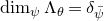 $\dim_{\psi}\Lambda_\theta= \delta_{\bar \psi}$
by Corollary 9.9, the claim follows.
$\dim_{\psi}\Lambda_\theta= \delta_{\bar \psi}$
by Corollary 9.9, the claim follows.
Applying Theorem 10.8 to each $\chi_{\alpha}$
,
$\chi_{\alpha}$
, $\alpha\in \theta$
, we obtain the following uniform lower bound on the Hausdorff dimension of all non-elementary
$\alpha\in \theta$
, we obtain the following uniform lower bound on the Hausdorff dimension of all non-elementary $\theta$
-Anosov subgroups.
$\theta$
-Anosov subgroups.
Corollary 10.9. We have
 $$\dim \Lambda_{\theta} \ge \max_{\alpha \in \theta} \delta_{\chi_{\alpha} + \chi_{{\rm i}(\alpha)}}.$$
Example 10.10. For $G = \operatorname{{\rm PSL}}_n(\mathbb R)$
, we have
$G = \operatorname{{\rm PSL}}_n(\mathbb R)$
, we have $\Pi = \{\alpha_1, \ldots, \alpha_{n-1} \},$
where
$\Pi = \{\alpha_1, \ldots, \alpha_{n-1} \},$
where
 $$\alpha_i : \operatorname{{\rm diag}}(a_1, \ldots, a_n) \mapsto a_i - a_{i+1} .$$
Let $1\le p\le n-1$
. Since
$1\le p\le n-1$
. Since $\chi_{\alpha_p}$
is equal to the fundamental weight
$\chi_{\alpha_p}$
is equal to the fundamental weight $\omega_p,$
which is given by
$\omega_p,$
which is given by $\omega_p(\operatorname{{\rm diag}}(a_1, \ldots, a_n))= a_1 + \cdots + a_p$
, we deduce from Corollary 10.9 that for all non-elementary
$\omega_p(\operatorname{{\rm diag}}(a_1, \ldots, a_n))= a_1 + \cdots + a_p$
, we deduce from Corollary 10.9 that for all non-elementary $\alpha_p$
-Anosov subgroups of
$\alpha_p$
-Anosov subgroups of $\operatorname{{\rm PSL}}_n(\mathbb R)$
, we have
$\operatorname{{\rm PSL}}_n(\mathbb R)$
, we have
 $$\dim \Lambda_{\alpha_p} \ge \delta_{\omega_p+ \omega_{n-p}}.$$
When $p = 1$
, this lower bound is obtained in [Reference Dey and KapovichDK22, Theorem 10.1].
$p = 1$
, this lower bound is obtained in [Reference Dey and KapovichDK22, Theorem 10.1].
The following upper bound in Proposition 10.11 was obtained in [Reference Pozzetti, Sambarino and WienhardPSW23, Theorem B] and [Reference Canary, Zhang and ZimmerCZZ26, Theorem 1.2] for $G = \operatorname{{\rm PSL}}_n(\mathbb R)$
and
$G = \operatorname{{\rm PSL}}_n(\mathbb R)$
and $\theta$
is a singleton.
$\theta$
is a singleton.
Proposition 10.11. We have
 $$ \dim \Lambda_{\theta} \le \max_{\alpha\in \theta}\delta_{\alpha} .$$
Proof. Via the proper immersion of $\mathcal F_{\theta}$
into
$\mathcal F_{\theta}$
into $\prod_{\alpha \in \theta} \mathbb{P}(V_{\alpha})$
as discussed in (10.4), we may consider the following metric on
$\prod_{\alpha \in \theta} \mathbb{P}(V_{\alpha})$
as discussed in (10.4), we may consider the following metric on $\mathcal F_{\theta}$
: for
$\mathcal F_{\theta}$
: for $g_1, g_2 \in G$
,
$g_1, g_2 \in G$
,
 $$d_{\mathcal F_\theta} (g_1 P_{\theta}, g_2 P_{\theta}) = \max_{\alpha \in \theta} d_{\mathbb{P}(V_{\alpha})}(g_1 V_{\alpha}^+, g_2 V_{\alpha}^+),$$
where $d_{\mathbb{P}(V_{\alpha})}$
is the metric on
$d_{\mathbb{P}(V_{\alpha})}$
is the metric on $\mathbb{P}(V_{\alpha})$
given by
$\mathbb{P}(V_{\alpha})$
given by $d_{\mathbb{P}(V_{\alpha})}(v_1, v_2) = \sin \angle (v_1, v_2)$
. Then,
$d_{\mathbb{P}(V_{\alpha})}(v_1, v_2) = \sin \angle (v_1, v_2)$
. Then, $d_{\mathcal F_{\theta}}$
is Lipschitz equivalent to the Riemannian distance on
$d_{\mathcal F_{\theta}}$
is Lipschitz equivalent to the Riemannian distance on $\mathcal F_\theta$
and hence we can use
$\mathcal F_\theta$
and hence we can use $d_{\mathcal F_{\theta}}$
to compute
$d_{\mathcal F_{\theta}}$
to compute $\dim \Lambda_{\theta}$
.
$\dim \Lambda_{\theta}$
.
Fix $\alpha\in \theta$
and consider the Tits representation
$\alpha\in \theta$
and consider the Tits representation $(\rho_\alpha, V_\alpha)$
. We write
$(\rho_\alpha, V_\alpha)$
. We write $V_\alpha=\mathbb R^{n_\alpha}$
and
$V_\alpha=\mathbb R^{n_\alpha}$
and $\operatorname{{\rm PGL}}(V_{\alpha})=\operatorname{{\rm PGL}}_{n_\alpha}(\mathbb R)$
by fixing a basis. We denote by
$\operatorname{{\rm PGL}}(V_{\alpha})=\operatorname{{\rm PGL}}_{n_\alpha}(\mathbb R)$
by fixing a basis. We denote by $\beta_{1,\alpha}$
the simple root of
$\beta_{1,\alpha}$
the simple root of $\operatorname{{\rm PGL}}_{n_\alpha}(\mathbb R)$
given by
$\operatorname{{\rm PGL}}_{n_\alpha}(\mathbb R)$
given by $\beta_{1,\alpha}(\operatorname{{\rm diag}}(u_1, \ldots, u_{n_\alpha}))=u_1-u_2.$
Since the highest weight of
$\beta_{1,\alpha}(\operatorname{{\rm diag}}(u_1, \ldots, u_{n_\alpha}))=u_1-u_2.$
Since the highest weight of $\rho_\alpha$
is
$\rho_\alpha$
is $\chi_{\alpha}$
and the second highest weight is
$\chi_{\alpha}$
and the second highest weight is $\chi_{\alpha}-\alpha $
by Theorem 10.1, we have that for all
$\chi_{\alpha}-\alpha $
by Theorem 10.1, we have that for all $\gamma\in \Gamma$
,
$\gamma\in \Gamma$
,
 \begin{equation} \beta_{1,\alpha}(\mu(\rho_{\alpha}(\gamma))) = \alpha(\mu(\gamma)).\end{equation}
Since $\Gamma$
is an
$\Gamma$
is an $\{\alpha\}$
-Anosov subgroup of G, there exists
$\{\alpha\}$
-Anosov subgroup of G, there exists $C\gt 1$
such that for all
$C\gt 1$
such that for all $\gamma \in \Gamma$
,
$\gamma \in \Gamma$
, $\alpha(\mu(\gamma)) \ge C^{-1}|\gamma|-C $
, and hence
$\alpha(\mu(\gamma)) \ge C^{-1}|\gamma|-C $
, and hence $\beta_{1,\alpha}(\mu(\rho_{\alpha}(\gamma))) \ge C^{-1}|\gamma|-C$
. Therefore,
$\beta_{1,\alpha}(\mu(\rho_{\alpha}(\gamma))) \ge C^{-1}|\gamma|-C$
. Therefore, $\rho_\alpha (\Gamma)$
is a
$\rho_\alpha (\Gamma)$
is a $\{\beta_{1, \rho}\}$
-Anosov subgroup of
$\{\beta_{1, \rho}\}$
-Anosov subgroup of $\operatorname{{\rm PGL}}_{n_\alpha}(\mathbb R)$
.
$\operatorname{{\rm PGL}}_{n_\alpha}(\mathbb R)$
.
We denote by $f_{\alpha} : \partial \Gamma \to \mathbb{P}(V_{\alpha})$
the
$f_{\alpha} : \partial \Gamma \to \mathbb{P}(V_{\alpha})$
the $\rho_{\alpha}(\Gamma)$
-equivariant embedding obtained as the extension of the orbit map of
$\rho_{\alpha}(\Gamma)$
-equivariant embedding obtained as the extension of the orbit map of $\rho_{\alpha}(\Gamma)$
(Theorem 3.8(4)). It is shown in [Reference Pozzetti, Sambarino and WienhardPSW23, Proposition 3.5, Proposition 3.8] that there exists a constant
$\rho_{\alpha}(\Gamma)$
(Theorem 3.8(4)). It is shown in [Reference Pozzetti, Sambarino and WienhardPSW23, Proposition 3.5, Proposition 3.8] that there exists a constant $C_{\alpha} \gt 0$
such that for each
$C_{\alpha} \gt 0$
such that for each $\gamma \in \Gamma$
, there exists a ball
$\gamma \in \Gamma$
, there exists a ball $\mathcal {B}_{\alpha}(\gamma)$
of radius
$\mathcal {B}_{\alpha}(\gamma)$
of radius $C_{\alpha} e^{-\beta_{1, \rho}(\mu(\rho_{\alpha}(\gamma)))}$
in
$C_{\alpha} e^{-\beta_{1, \rho}(\mu(\rho_{\alpha}(\gamma)))}$
in $\mathbb{P}(V_{\alpha})$
so that for any
$\mathbb{P}(V_{\alpha})$
so that for any $x \in \partial \Gamma$
such that
$x \in \partial \Gamma$
such that $\gamma \in [e, x]$
in
$\gamma \in [e, x]$
in $\Gamma$
, we have
$\Gamma$
, we have $f_{\alpha}(x) \in \mathcal {B}_{\alpha}(\gamma)$
. In particular, for every
$f_{\alpha}(x) \in \mathcal {B}_{\alpha}(\gamma)$
. In particular, for every $k \ge 1$
, the collection
$k \ge 1$
, the collection
 $$\{\mathcal {B}_{\alpha}(\gamma) : \gamma \in \Gamma, \ |\gamma| = k \}$$
covers the limit set of $\rho_{\alpha}(\Gamma)$
in
$\rho_{\alpha}(\Gamma)$
in $\mathbb{P}(V_{\alpha})$
. Hence,
$\mathbb{P}(V_{\alpha})$
. Hence, $\Lambda_{\theta}$
is covered by the collection
$\Lambda_{\theta}$
is covered by the collection
 $$\bigg\{\prod_{\alpha \in \theta} \mathcal {B}_{\alpha}(\gamma) : \gamma \in \Gamma, |\gamma| = k \bigg\}$$
via the immersion $\mathcal F_{\theta} \to \prod_{\alpha \in \theta} \mathbb{P}(V_{\alpha})$
. Since
$\mathcal F_{\theta} \to \prod_{\alpha \in \theta} \mathbb{P}(V_{\alpha})$
. Since $\prod_{\alpha \in \theta} \mathcal {B}_{\alpha}(\gamma)$
has
$\prod_{\alpha \in \theta} \mathcal {B}_{\alpha}(\gamma)$
has $d_{\mathcal F_\theta}$
-diameter at most
$d_{\mathcal F_\theta}$
-diameter at most
 $$\max_{\alpha \in \theta} C_{\alpha} e^{-\beta_{1, \rho}(\mu(\rho_{\alpha}(\gamma)))} \le C e^{-\min_{\alpha \in \theta} \alpha(\mu(\gamma))},$$
where $C = \max_{\alpha \in \theta} C_{\alpha}$
by (10.8), we have that for each
$C = \max_{\alpha \in \theta} C_{\alpha}$
by (10.8), we have that for each $s \gt 0$
, the s-dimensional Hausdorff measure
$s \gt 0$
, the s-dimensional Hausdorff measure $\mathcal H^s(\Lambda_\theta)$
with respect to
$\mathcal H^s(\Lambda_\theta)$
with respect to $d_{\mathcal F_\theta}$
satisfies
$d_{\mathcal F_\theta}$
satisfies
 $$\mathcal H^s(\Lambda_\theta) \le \limsup_{k \to \infty} C^s \sum_{\gamma \in \Gamma, |\gamma| = k} e^{-s \min_{\alpha \in \theta} \alpha(\mu(\gamma))}.$$
Therefore, denoting by $\delta_{\min_{\alpha \in \theta} \alpha}$
the abscissa of convergence of the series
$\delta_{\min_{\alpha \in \theta} \alpha}$
the abscissa of convergence of the series $s \mapsto \sum_{\gamma \in \Gamma} e^{-s \min_{\alpha \in \theta} \alpha(\mu(\gamma))}$
, if
$s \mapsto \sum_{\gamma \in \Gamma} e^{-s \min_{\alpha \in \theta} \alpha(\mu(\gamma))}$
, if $s \gt \delta_{\min_{\alpha \in \theta} \alpha}$
, we have
$s \gt \delta_{\min_{\alpha \in \theta} \alpha}$
, we have $ \mathcal H^s(\Lambda_\theta)=0$
and hence
$ \mathcal H^s(\Lambda_\theta)=0$
and hence
 $$\dim \Lambda_{\theta} \le \delta_{\min_{\alpha \in \theta} \alpha}.$$
On the other hand, we have
 $$\frac{1}{\# \theta} \sum_{\alpha \in \theta} \sum_{\gamma \in \Gamma} e^{- s \alpha(\mu(\gamma))} \le \sum_{\gamma \in \Gamma} e^{-s \min_{\alpha \in \theta} \alpha(\mu(\gamma))} \le \sum_{\alpha \in \theta} \sum_{\gamma \in \Gamma} e^{-s \alpha(\mu(\gamma))}.$$
The first inequality implies $\max_{\alpha \in \theta} \delta_{\alpha} \le \delta_{\min_{\alpha \in \theta} \alpha}$
and the second gives
$\max_{\alpha \in \theta} \delta_{\alpha} \le \delta_{\min_{\alpha \in \theta} \alpha}$
and the second gives $\delta_{\min_{\alpha \in \theta} \alpha} \le \max_{\alpha \in \theta} \delta_{\alpha}$
. Hence,
$\delta_{\min_{\alpha \in \theta} \alpha} \le \max_{\alpha \in \theta} \delta_{\alpha}$
. Hence, $\delta_{\min_{\alpha \in \theta} \alpha} = \max_{\alpha \in \theta} \delta_{\alpha}$
, which completes the proof.
$\delta_{\min_{\alpha \in \theta} \alpha} = \max_{\alpha \in \theta} \delta_{\alpha}$
, which completes the proof.
Theorem 1.7 is a combination of Corollary 10.9 and Proposition 10.11.
11. Growth indicator bounds and applications to the
$L^2$
-spectrum

As before, let $\Gamma\lt G$
be a
$\Gamma\lt G$
be a $\theta$
-Anosov subgroup where G is a connected semisimple real algebraic group. In this final section, we deduce bounds on the growth indicator
$\theta$
-Anosov subgroup where G is a connected semisimple real algebraic group. In this final section, we deduce bounds on the growth indicator $\psi_\Gamma^\theta:\mathfrak a_\theta\to [0, \infty)\cup\{-\infty\}$
of
$\psi_\Gamma^\theta:\mathfrak a_\theta\to [0, \infty)\cup\{-\infty\}$
of $\Gamma$
(see Definition 3.1) from Corollary 10.9. Recall Tits weights
$\Gamma$
(see Definition 3.1) from Corollary 10.9. Recall Tits weights $\chi_\alpha$
,
$\chi_\alpha$
, $\alpha\in \Pi$
, of G from (10.2). We have the following (Corollary 1.8).
$\alpha\in \Pi$
, of G from (10.2). We have the following (Corollary 1.8).
Corollary 11.1. We have
 \begin{equation} \psi_{\Gamma}^{\theta \cup {\rm i}(\theta)} \le \dim \Lambda_{\theta} \cdot \min_{\alpha \in \theta} (\chi_{\alpha} + \chi_{{\rm i}(\alpha)}). \end{equation}
Moreover,
 \begin{equation} \psi_{\Gamma} \le \dim \Lambda_{\theta} \cdot \min_{\alpha \in \theta} (\chi_{\alpha} + \chi_{{\rm i}(\alpha)}).\end{equation}
Proof. For any linear form $\psi\in \mathfrak a_{\theta \cup {\rm i}(\theta)}^*$
positive on
$\psi\in \mathfrak a_{\theta \cup {\rm i}(\theta)}^*$
positive on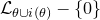 $\mathcal L_{\theta \cup {\rm i}(\theta)} - \{0\}$
, the scaled linear from
$\mathcal L_{\theta \cup {\rm i}(\theta)} - \{0\}$
, the scaled linear from $\delta_{\psi} \psi$
is tangent to the growth indicator (Lemma 3.6). Hence it follows from Corollary 10.9 that for each
$\delta_{\psi} \psi$
is tangent to the growth indicator (Lemma 3.6). Hence it follows from Corollary 10.9 that for each $\alpha \in \theta$
, we have
$\alpha \in \theta$
, we have
 $$ \psi_{\Gamma}^{\theta \cup {\rm i}(\theta)} \le \delta_{\chi_{\alpha} + \chi_{{\rm i}(\alpha)}} \cdot (\chi_{\alpha} + \chi_{{\rm i}(\alpha)}) \le \dim \Lambda_{\theta} \cdot (\chi_{\alpha} + \chi_{{\rm i}(\alpha)}) \quad \text{on } \mathfrak a_{\theta \cup {\rm i}(\theta)}. $$
Therefore, taking the minimum among $\alpha \in \theta$
finishes the proof of (11.1).
$\alpha \in \theta$
finishes the proof of (11.1).
By [Reference Kim, Oh and WangKOW25b, Lemma 3.12], we have
 $$\psi_{\Gamma} \le \psi_{\Gamma}^{\theta \cup {\rm i}(\theta)} \circ p_{\theta \cup {\rm i}(\theta)}\quad\text{on } \mathfrak a.$$
Hence, by (11.1), we have
 $$\psi_{\Gamma} \le \dim \Lambda_{\theta} \cdot \min_{\alpha \in \theta} (\chi_{\alpha} + \chi_{{\rm i}(\alpha)}) \circ p_{\theta \cup {\rm i}(\theta)}.$$
Since the linear form $\chi_{\alpha} + \chi_{{\rm i}(\alpha)} \in \mathfrak a_{\theta \cup {\rm i}(\theta)}^*$
is
$\chi_{\alpha} + \chi_{{\rm i}(\alpha)} \in \mathfrak a_{\theta \cup {\rm i}(\theta)}^*$
is $p_{\theta \cup {\rm i}(\theta)}$
-invariant for each
$p_{\theta \cup {\rm i}(\theta)}$
-invariant for each $\alpha \in \theta$
, (11.2) follows.
$\alpha \in \theta$
, (11.2) follows.
Observing
 $$\min_{\alpha \in \theta} (\chi_{\alpha} + \chi_{{\rm i}(\alpha)} ) \le \frac{1}{\# \theta} \sum_{\alpha \in \theta} \chi_{\alpha} + \chi_{{\rm i}(\alpha)},$$
Corollary 11.1 implies the following.
Corollary 11.2.
For any $\theta$
-Anosov subgroup of G, we have
$\theta$
-Anosov subgroup of G, we have
 \begin{equation} \psi_{\Gamma} \le \frac{{\mathsf c}_\theta \dim \Lambda_{\theta}}{\# \theta }\cdot \rho .\end{equation}
Remark 11.3. We remark that our proof shows that ${{\mathsf c}_\theta }/{\# \theta }$
in the above corollary can be replaced by the minimum
${{\mathsf c}_\theta }/{\# \theta }$
in the above corollary can be replaced by the minimum $c\ge 0$
such that
$c\ge 0$
such that $\min_{\alpha \in \theta} ( \chi_{\alpha} + \chi_{{\rm i}(\alpha)} ) \le c \cdot \rho $
on the limit cone
$\min_{\alpha \in \theta} ( \chi_{\alpha} + \chi_{{\rm i}(\alpha)} ) \le c \cdot \rho $
on the limit cone $\mathcal L$
.
$\mathcal L$
.
Define the real number $\lambda_0(\Gamma\backslash X) \in [0,\infty)$
as follows:
$\lambda_0(\Gamma\backslash X) \in [0,\infty)$
as follows:
 \begin{equation} \lambda_0(\Gamma\backslash X):= \inf\left\lbrace \frac{\int_{\Gamma\backslash X}\|\text{grad} \, f \|^2\,d\operatorname{Vol}}{\int_{\Gamma\backslash X}|f|^2\,d\operatorname{Vol}}\,:\,f\in C^\infty_c(\Gamma\backslash X),\; f\neq 0 \right\rbrace\!.\end{equation}
This number is equal to the bottom of the $L^2$
-spectrum of
$L^2$
-spectrum of $\Gamma \backslash X$
of the Laplace–Beltrami operator [Reference SullivanSul87, Theorem 2.2]. The following was proved in [Reference Edwards and OhEO23, Theorem 1.6] for
$\Gamma \backslash X$
of the Laplace–Beltrami operator [Reference SullivanSul87, Theorem 2.2]. The following was proved in [Reference Edwards and OhEO23, Theorem 1.6] for $\Pi$
-Anosov subgroups and in [Reference Lutsko, Weich and WolfLWW24, Corollary 3] in general.
$\Pi$
-Anosov subgroups and in [Reference Lutsko, Weich and WolfLWW24, Corollary 3] in general.
Theorem 11.4.
If $\Gamma\lt G$
is a torsion-free discrete subgroup of G with
$\Gamma\lt G$
is a torsion-free discrete subgroup of G with $\psi_\Gamma \le \rho$
, then
$\psi_\Gamma \le \rho$
, then $L^2(\Gamma \backslash G)$
is tempered and
$L^2(\Gamma \backslash G)$
is tempered and $\lambda_0(\Gamma\backslash X) = \| \rho\|^2$
.
$\lambda_0(\Gamma\backslash X) = \| \rho\|^2$
.
Applying Theorem 11.4, we obtain the following (Corollary 1.9) from (11.3).
Corollary 11.5.
Let $\Gamma$
be a torsion-free
$\Gamma$
be a torsion-free $\theta$
-Anosov subgroup. If
$\theta$
-Anosov subgroup. If $ \dim \Lambda_{\theta} \le {\# \theta}/{{\mathsf c}_\theta}$
, then
$ \dim \Lambda_{\theta} \le {\# \theta}/{{\mathsf c}_\theta}$
, then $L^2(\Gamma \backslash G)$
is tempered and
$L^2(\Gamma \backslash G)$
is tempered and $\lambda_0(\Gamma\backslash X) = \| \rho\|^2$
.
$\lambda_0(\Gamma\backslash X) = \| \rho\|^2$
.
Moreover, $\lambda_0$
is not an
$\lambda_0$
is not an $L^2$
-eigenvalue [Reference Edwards and OhEO23, Reference Edwards, Fraczyk, Lee and OhEFL+24] (see also [Reference Weich and WolfWW23, Corollary 5.2] for the absence of any principal joint
$L^2$
-eigenvalue [Reference Edwards and OhEO23, Reference Edwards, Fraczyk, Lee and OhEFL+24] (see also [Reference Weich and WolfWW23, Corollary 5.2] for the absence of any principal joint $L^2$
-eigenvalues as well).
$L^2$
-eigenvalues as well).
Remark 11.6. Indeed, it is shown in [Reference Lutsko, Weich and WolfLWW24, Theorem 11] that if $\psi_\Gamma \le (2-{2}/{p}) \rho$
for some
$\psi_\Gamma \le (2-{2}/{p}) \rho$
for some $p \ge 1$
, then
$p \ge 1$
, then $L^2(\Gamma\backslash G)$
is strongly
$L^2(\Gamma\backslash G)$
is strongly $L^{p+\varepsilon}$
-integrable for all
$L^{p+\varepsilon}$
-integrable for all $\varepsilon\gt 0$
; that is, for a dense subset of vectors, the associated matrix coefficients belong to
$\varepsilon\gt 0$
; that is, for a dense subset of vectors, the associated matrix coefficients belong to $L^{p+\varepsilon}(G)$
. Hence, if
$L^{p+\varepsilon}(G)$
. Hence, if $ \dim \Lambda_{\theta} \le (2- {2}/p) {\# \theta}/{{\mathsf c}_\theta}$
, we obtain that
$ \dim \Lambda_{\theta} \le (2- {2}/p) {\# \theta}/{{\mathsf c}_\theta}$
, we obtain that $L^2(\Gamma\backslash G)$
is strongly
$L^2(\Gamma\backslash G)$
is strongly $L^{p+\varepsilon}$
-integrable for all
$L^{p+\varepsilon}$
-integrable for all $\varepsilon\gt 0$
.
$\varepsilon\gt 0$
.
Remark 11.7. Using that $\mathsf c_G = {2}/({n-1})$
for
$\mathsf c_G = {2}/({n-1})$
for $G = \operatorname{{\rm SO}}^\circ(n, 1)$
, Corollary 11.5 says that for a Zariski dense convex cocompact
$G = \operatorname{{\rm SO}}^\circ(n, 1)$
, Corollary 11.5 says that for a Zariski dense convex cocompact $\Gamma \lt \operatorname{{\rm SO}}^\circ(n, 1)$
, if
$\Gamma \lt \operatorname{{\rm SO}}^\circ(n, 1)$
, if $\dim \Lambda \le ({n-1})/{2}$
, then
$\dim \Lambda \le ({n-1})/{2}$
, then $L^2(\Gamma \backslash \operatorname{{\rm SO}}^\circ(n, 1))$
is tempered and
$L^2(\Gamma \backslash \operatorname{{\rm SO}}^\circ(n, 1))$
is tempered and $\lambda_0(\Gamma \backslash \mathbb H^n) = {(n-1)^2}/{4}$
, as shown by Sullivan [Reference SullivanSul87, Theorem 2.21].
$\lambda_0(\Gamma \backslash \mathbb H^n) = {(n-1)^2}/{4}$
, as shown by Sullivan [Reference SullivanSul87, Theorem 2.21].
Acknowledgement
We would like to thank Ilia Smilga for providing the proof of Lemma 10.3.
Conflicts of interest
None.
Financial support
Oh is partially supported by the NSF grant no. DMS-1900101 and 2450703.
Journal information
Compositio Mathematica is owned by the Foundation Compositio Mathematica and published by the London Mathematical Society in partnership with Cambridge University Press. All surplus income from the publication of Compositio Mathematica is returned to mathematics and higher education through the charitable activities of the Foundation, the London Mathematical Society and Cambridge University Press.













 a
a
 C′
C′ a+
a+

 γo
γo vjo
vjo vj−n′o
 uko
uko

 [ξ,η]o
 [e,η]o
 η
η OT′+D0θ(o,go)

 Open access

