


1. Introduction
Non-spherical particles are ubiquitous in numerous natural and industrial processes, including pollen transmission (Sabban & van Hout Reference Sabban and van Hout2011), biomass combustion (Cui & Grace Reference Cui and Grace2007), papermaking processes (Lundell, Söderberg & Alfredsson Reference Lundell, Söderberg and Alfredsson2011) and drug delivery (Kleinstreuer & Feng Reference Kleinstreuer and Feng2013), just to name a few. Understanding their hydrodynamic behaviour near walls is of paramount importance, as in most realistic scenarios, particles interact with boundaries rather than exist in unbounded flows. Although significant progress has been made in characterising the dynamics of spherical particles near a wall (Brenner Reference Brenner1961; Goldman, Cox & Brenner Reference Goldman, Cox and Brenner1967; Cox & Hsu Reference Cox and Hsu1977; Huang et al. Reference Huang, Lin, Wang, Li, Jin and Shao2025), the behaviour of non-spherical particles in such confined configurations remains inadequately understood (Bhagat & Goswami Reference Bhagat and Goswami2022). This knowledge gap stems from the complex, nonlinear coupling among particle Reynolds number, wall distance, aspect ratio and orientation, which collectively govern the forces and torques acting on particles and pose significant challenges for prediction in wall-bounded flows, where confinement effects and wake–boundary interactions alter force distributions and scaling behaviours.
Extensive research has been devoted to understanding the hydrodynamic behaviour of non-spherical particles in fluid flows. Early studies focused on mechanisms such as particle settling (Tinklenberg, Guala & Coletti Reference Tinklenberg, Guala and Coletti2024; Peng et al. Reference Peng, Karzhaubayev, Wang, Chen and Niu2025), the statistical characterisation of the particle dynamics (Allende & Bec Reference Allende and Bec2023; Dahlkild Reference Dahlkild2023; Anand & Ray Reference Anand and Ray2025), interactions between wall-bounded turbulence and non-spherical particles (Zhang et al. Reference Zhang, Guo, Peng and Wang2025) and stability analysis (Cui et al. Reference Cui, Jiang, Qiu and Zhao2025). These works have provided fundamental insights into how particle shape and orientation interact with local flow structures, influencing key mechanisms of drag, lift and torque generation. Building on these insights, substantial research efforts have focused on the quantitative prediction of the corresponding hydrodynamic coefficients, which are essential for accurate modelling of particle motion in complex flows. Loth (Reference Loth2008) systematically reviewed drag correlations for regular and irregular particles across Stokes and Newtonian regimes, highlighting the limitations of using sphericity as a universal predictor, especially at intermediate Reynolds numbers. To address this, Hölzer & Sommerfeld (Reference Hölzer and Sommerfeld2008, Reference Hölzer and Sommerfeld2009) developed improved empirical correlations incorporating projected area to account for orientation effects. Subsequently, Zastawny et al. (Reference Zastawny, Mallouppas, Zhao and Van Wachem2012) applied the immersed boundary method (IBM) to study ellipsoids and fibres over a range of orientations and Reynolds numbers, deriving geometry-dependent correlations for drag, lift and torque. However, due to limited domain sizes at low Reynolds number (
 $ \textit{Re}$
), where
$ \textit{Re}$
), where
 $ \textit{Re} \leqslant 1$
, their accuracy in the Stokes regime was compromised (Zastawny et al. Reference Zastawny, Mallouppas, Zhao and Van Wachem2012; Ouchene et al. Reference Ouchene, Khalij, Arcen and Tanière2016).
$ \textit{Re} \leqslant 1$
, their accuracy in the Stokes regime was compromised (Zastawny et al. Reference Zastawny, Mallouppas, Zhao and Van Wachem2012; Ouchene et al. Reference Ouchene, Khalij, Arcen and Tanière2016).
Early shape descriptors such as sphericity (Wadell Reference Wadell1934) mapped non-spherical particles to volume-equivalent spheres but ignored orientation – a critical shortcoming, since particles with identical sphericity can exhibit markedly different aerodynamic behaviours. Although Hölzer & Sommerfeld (Reference Hölzer and Sommerfeld2008) introduced a modified sphericity parameter, it still performed poorly for highly elongated or flattened shapes (Ouchene et al. Reference Ouchene, Khalij, Tanière and Arcen2015). Analytical progress was made by Happel & Brenner (Reference Happel and Brenner1983), who expressed the drag coefficient at arbitrary incidence as a function of extreme-orientation values (
 $0^\circ$
and
$0^\circ$
and
 $90^\circ$
) modulated by a
$90^\circ$
) modulated by a
 $\sin ^2$
dependence on the angle. This sine-squared scaling, rooted in axisymmetric resistance tensors in Stokes flow, has shown reasonable accuracy at moderate
$\sin ^2$
dependence on the angle. This sine-squared scaling, rooted in axisymmetric resistance tensors in Stokes flow, has shown reasonable accuracy at moderate
 $ \textit{Re}$
(Sanjeevi & Padding Reference Sanjeevi and Padding2017). Recent studies using IBM and lattice Boltzmann methods (LBM) have extended such correlations to
$ \textit{Re}$
(Sanjeevi & Padding Reference Sanjeevi and Padding2017). Recent studies using IBM and lattice Boltzmann methods (LBM) have extended such correlations to
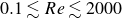 $0.1 \lesssim Re \lesssim 2000$
(Zastawny et al. Reference Zastawny, Mallouppas, Zhao and Van Wachem2012; Sanjeevi, Kuipers & Padding Reference Sanjeevi, Kuipers and Padding2018). However, these models largely neglect wall effects, where wall proximity may break symmetry or introduce higher-order angular dependencies.
$0.1 \lesssim Re \lesssim 2000$
(Zastawny et al. Reference Zastawny, Mallouppas, Zhao and Van Wachem2012; Sanjeevi, Kuipers & Padding Reference Sanjeevi, Kuipers and Padding2018). However, these models largely neglect wall effects, where wall proximity may break symmetry or introduce higher-order angular dependencies.
Recent numerical investigations have begun to address this gap. Fillingham et al. (Reference Fillingham, Vaddi, Bruning, Israel and Novosselov2021) simulated horizontally oriented ellipsoids in smooth-wall contact for
 $0.1 \leqslant Re \leqslant 10$
and proposed corresponding drag correlations. Similarly, De Souza, Ouchene & Thomas (Reference De Souza, Ouchene and Thomas2024) observed a robust
$0.1 \leqslant Re \leqslant 10$
and proposed corresponding drag correlations. Similarly, De Souza, Ouchene & Thomas (Reference De Souza, Ouchene and Thomas2024) observed a robust
 $\sin ^2$
dependence for oblate spheroids in direct wall contact, suggesting the potential persistence of this scaling under confinement. Using the LBM, Gao et al. (Reference Gao, Hu, Meng, Cui, Mao and Liu2025) studied wall-attached ellipsoids in shear flow, examining orientation, aspect ratio and Reynolds-number effects, and proposed detachment criteria. For oblate ellipsoids, Cao et al. (Reference Cao, Li, Liu, Zhang, Tafti, Wang, Yuan and Hu2025) extended the Reynolds-number range and developed drag models for various vertical angles. Despite these advances, existing studies are largely restricted to particles in direct wall contact, leaving the influence of finite wall distance still largely unexplored.
$\sin ^2$
dependence for oblate spheroids in direct wall contact, suggesting the potential persistence of this scaling under confinement. Using the LBM, Gao et al. (Reference Gao, Hu, Meng, Cui, Mao and Liu2025) studied wall-attached ellipsoids in shear flow, examining orientation, aspect ratio and Reynolds-number effects, and proposed detachment criteria. For oblate ellipsoids, Cao et al. (Reference Cao, Li, Liu, Zhang, Tafti, Wang, Yuan and Hu2025) extended the Reynolds-number range and developed drag models for various vertical angles. Despite these advances, existing studies are largely restricted to particles in direct wall contact, leaving the influence of finite wall distance still largely unexplored.
Only a handful of studies have considered finite clearance. Gavze & Shapiro (Reference Gavze and Shapiro1997) used a boundary integral method under Stokes-flow conditions to analyse ellipsoids in shear near a wall, finding that wall-induced drag enhancement decreases with increasing particle asphericity. More recently, Bhagat & Goswami (Reference Bhagat and Goswami2022) examined spheroids near a rough wall at moderate Reynolds number (
 $10 \leqslant Re \leqslant 100$
), focusing on vertical orientation. Similarly, Chéron & van Wachem (Reference Chéron and van Wachem2024) performed direct numerical simulations (DNSs) of rod-like particles to assess the effects of wall distance, aspect ratio, orientation and
$10 \leqslant Re \leqslant 100$
), focusing on vertical orientation. Similarly, Chéron & van Wachem (Reference Chéron and van Wachem2024) performed direct numerical simulations (DNSs) of rod-like particles to assess the effects of wall distance, aspect ratio, orientation and
 $ \textit{Re}$
, observing strong near-wall drag amplification and proposing an empirical correlation.
$ \textit{Re}$
, observing strong near-wall drag amplification and proposing an empirical correlation.
Machine-learning techniques have been widely adopted across fluid dynamics research (Ling, Kurzawski & Templeton Reference Ling, Kurzawski and Templeton2016; Kutz Reference Kutz2017; Duraisamy, Iaccarino & Xiao Reference Duraisamy, Iaccarino and Xiao2019; Brunton, Noack & Koumoutsakos Reference Brunton, Noack and Koumoutsakos2020; Bae & Koumoutsakos Reference Bae and Koumoutsakos2022; Taira, Rigas & Fukami Reference Taira, Rigas and Fukami2025), with applications spanning flow-field estimation (Fukami et al. Reference Fukami, Maulik, Ramachandra, Fukagata and Taira2021b ; Cuellar et al. Reference Cuellar, Guemes, Ianiro, Flores, Vinuesa and Discetti2025), super-resolution reconstruction (Kim et al. Reference Kim, Kim, Won and Lee2021; Fukami et al. Reference Fukami, Fukagata and Taira2021a ; Maejima & Kawai Reference Maejima and Kawai2025; Page Reference Page2025; Dong et al. Reference Dong, Zhang, Xiao and Mao2025), reduced order modelling (Brunton et al. Reference Brunton, Noack and Koumoutsakos2020), flow control (Rabault et al. Reference Rabault, Kuchta, Jensen, Rëglade and Cerardi2019; Park & Choi Reference Park and Choi2020) and turbulence modelling (Ling et al. Reference Ling, Kurzawski and Templeton2016; Duraisamy et al. Reference Duraisamy, Iaccarino and Xiao2019; Xie et al. Reference Xie, Wang and E2020, Reference Xie, Xiong and Wang2021; Zhang et al. Reference Zhang, Xiao, Luo and He2022; List, Chen & Thuerey Reference List, Chen and Thuerey2022; Xu et al. Reference Xu, Wang, Yu and Chen2023; Lozano-Durán & Bae Reference Lozano-Durán and Bae2023; Cho, Park & Choi Reference Cho, Park and Choi2024). With recent advancements in deep learning, neural networks have been increasingly applied to predict the hydrodynamic behaviour of particles.
Early machine-learning applications in this field include the work of Yan et al. (Reference Yan, He, Tang and Wang2019), who employed artificial neural networks (ANN) and radial basis function neural networks to predict drag coefficients of non-spherical particles. Their results showed good performance for nearly spherical particles but deteriorated accuracy for low-sphericity shapes. Subsequently, Tajfirooz et al. (Reference Tajfirooz, Meijer, Kuerten, Hausmann, Fröhlich and Zeegers2021) developed a multilayer perceptron model for ellipsoidal particles using the Reynolds number (
 $0.25 \leqslant Re \leqslant 250$
) and orientation angle (
$0.25 \leqslant Re \leqslant 250$
) and orientation angle (
 $0^{\circ } \leqslant \alpha \leqslant 90^{\circ }$
) as inputs to simultaneously predict drag, lift and moment coefficients, demonstrating superiority over conventional empirical correlations in point-particle simulations. Around the same period, Hwang, Pan & Fan (Reference Hwang, Pan and Fan2021) proposed a convolutional neural network (CNN) framework to predict hydrodynamic coefficients of ellipsoidal particles at low Reynolds number, validated against particle-resolved DNS data with excellent agreement.
$0^{\circ } \leqslant \alpha \leqslant 90^{\circ }$
) as inputs to simultaneously predict drag, lift and moment coefficients, demonstrating superiority over conventional empirical correlations in point-particle simulations. Around the same period, Hwang, Pan & Fan (Reference Hwang, Pan and Fan2021) proposed a convolutional neural network (CNN) framework to predict hydrodynamic coefficients of ellipsoidal particles at low Reynolds number, validated against particle-resolved DNS data with excellent agreement.
More recent studies have explored advanced architectures and hybrid approaches. Xiang et al. (Reference Xiang, Cheng, Zhang and Jiang2024) coupled discrete element method (DEM) with an improved velocity interpolation scheme in LBM, using high-fidelity DEM–LBM datasets to train a genetic algorithm optimised ANN that achieved mean relative errors below 5.0 % for arbitrary polygonal particles. Similarly, Wang et al. (Reference Wang, Ma, Fang, Zhang, Chen and Yin2024) introduced a hybrid machine-learning algorithm integrating multiple single-tree models with a convolutional layer, trained on 1092 datasets, achieving relative errors below 5.0 % for cylindrical bodies. Most recently, Presa-Reyes et al. (Reference Presa-Reyes, Mahyawansi, Hu, McDaniel and Chen2024) combined empirical correlations with deep neural networks (DNNs) in a drag coefficient correlation–DNN model, where classical relations were embedded within the DNN structure and multiple outputs were adaptively weighted using a gating network, significantly enhancing robustness, particularly in small-sample scenarios.
The interpretability of machine-learning models has gained increasing attention in fluid mechanics, with applications including turbulence modelling improvement (Mandler & Weigand Reference Mandler and Weigand2023), elucidation of fundamental physical mechanisms (Kim, Kim & Lee Reference Kim, Kim and Lee2023), turbulence assessment during aircraft descent (Khattak et al. Reference Khattak, Chan, Chen and Peng2023) and identification of two-phase flow regimes (Khan et al. Reference Khan, Pao, Pilario, Sallih and Khan2024). Among interpretability techniques, Shapley additive explanations (SHAPs) (Lundberg & Lee Reference Lundberg and Lee2017), grounded in cooperative game theory, provide both global and local insights by quantifying the marginal contribution of each input feature. This capability makes SHAP particularly valuable for enhancing the physical interpretability of data-driven models in fluid dynamics.
Recent applications of SHAP analysis in fluid mechanics include the work of Lellep et al. (Reference Lellep, Prexl, Eckhardt and Linkmann2022), who employed an XGBoost model to predict relaminarisation events in wall-bounded shear flows using a nine-mode model of Couette flow (Moehlis, Faisst & Eckhardt Reference Moehlis, Faisst and Eckhardt2004), with SHAP analysis revealing key modal interactions governing the process. Cremades et al. (Reference Cremades2024) applied a U-net architecture to predict the temporal evolution of turbulent channel flows and used SHAP to quantify the importance of different spatial regions, demonstrating that the method effectively identifies key dynamical regions associated with Reynolds-stress structures. Most recently, Hoyas et al. (Reference Hoyas, Benedikt, Cremades and Vinuesa2025) developed U-net-based CNNs for three-dimensional flow-field reconstruction and wall-shear-stress prediction in turbulent channel flows, employing kernel-SHAP to analyse the contribution of coherent flow structures to skin friction. The gradient-SHAP explainability algorithm provides an objective way to identify the regions of higher importance in a turbulent channel, which exhibit different levels of agreement with the classical structures without being completely related to any particular one (Cremades, Hoyas & Vinuesa Reference Cremades, Hoyas and Vinuesa2025).
Although existing studies have advanced our understanding of hydrodynamic behaviour around non-spherical particles, significant knowledge gaps remain (Marchioli et al. Reference Marchioli2025). Current research is often confined to specific particle shapes, orientations or flow regimes, with limited consideration of non-contact wall interactions. Furthermore, most machine-learning models developed for predicting drag, lift and torque coefficients treat these aerodynamic parameters as independent outputs, neglecting their potential intercorrelations – a limitation that may restrict the models’ capacity to capture the coupled physical interactions governing the particle–fluid dynamics. In realistic environments, particles seldom maintain permanent wall contact but typically experience varying clearance distances where wall-induced effects substantially modify hydrodynamic forces and trajectories. A deeper understanding of these mechanisms is crucial for enhancing predictive models in applications such as sedimentation, microfluidics, environmental dispersion and aerosol science.
The primary objective of this study is to develop a multi-stage physics-informed machine-learning (MSPIML) framework capable of accurately predicting the drag, lift and pitching torque coefficients of the prolate spheroid under finite wall-confinement conditions. To obtain high-fidelity data for model training, fully resolved DNSs are conducted, covering a wide range of parameters, including Reynolds numbers (
 $0.5\leqslant Re \leqslant 115$
), horizontal and vertical orientation angles (
$0.5\leqslant Re \leqslant 115$
), horizontal and vertical orientation angles (
 $\alpha _H$
,
$\alpha _H$
,
 $\alpha _V$
) and dimensionless wall distance
$\alpha _V$
) and dimensionless wall distance
 $G/D$
, where
$G/D$
, where
 $G$
is the minimum gap between the particle surface and the wall and
$G$
is the minimum gap between the particle surface and the wall and
 $D$
is the diameter of a volume-equivalent sphere for a spheroid, from near contact to the nearly unbounded limit. In the MSPIML framework, the drag coefficient is accurately predicted under physical constraints using a physics-informed mixture-of-experts (PIMoE) model that integrates classical empirical correlations with a statistical expert. The accurate drag coefficient prediction is incorporated as an additional input feature for the lift and pitching torque coefficient models. This hierarchical structure enriches the input space and enhances overall predictive accuracy. Finally, the SHAP method is employed to analyse the relationships between each input feature and the output of the MSPIML framework, providing direct insight into the decision-making basis of the model.
$D$
is the diameter of a volume-equivalent sphere for a spheroid, from near contact to the nearly unbounded limit. In the MSPIML framework, the drag coefficient is accurately predicted under physical constraints using a physics-informed mixture-of-experts (PIMoE) model that integrates classical empirical correlations with a statistical expert. The accurate drag coefficient prediction is incorporated as an additional input feature for the lift and pitching torque coefficient models. This hierarchical structure enriches the input space and enhances overall predictive accuracy. Finally, the SHAP method is employed to analyse the relationships between each input feature and the output of the MSPIML framework, providing direct insight into the decision-making basis of the model.
The remainder of this paper is organised as follows. Section 2 presents the governing equations, numerical set-up and the DNS results for the drag, lift and pitching torque coefficients. Section 3 details the empirical correlations and the modelling strategy. Section 4 introduces the MSPIML framework. Section 5 evaluates the predictive performance in detail and analyses model interpretability using SHAP. Finally, § 6 summarises the main findings and highlights directions for future work.
2. Numerical methodology
2.1. Governing equations and numerical framework
The flow past a stationary prolate spheroid in the vicinity of a plane wall is governed by the three-dimensional incompressible Navier–Stokes equations in Cartesian coordinates (Pope Reference Pope2000)
 \begin{align} \frac {\partial U_i}{\partial x_i} = 0, \\[-28pt] \nonumber \end{align}
 \begin{align} U_j \frac {\partial U_i}{\partial x_{\kern-1pt j}} = -\frac {1}{\rho _{\kern-1pt f}}\frac {\partial P}{\partial x_i} + \nu \frac {\partial ^2 U_i}{\partial x_{\kern-1pt j}^2}, \\[0pt] \nonumber \end{align}
where
 $x_i=(x,y,z)$
denotes the Cartesian coordinates,
$x_i=(x,y,z)$
denotes the Cartesian coordinates,
 $U_i$
the velocity components,
$U_i$
the velocity components,
 $P$
the pressure,
$P$
the pressure,
 $\rho _{\kern-1pt f}$
the fluid density and
$\rho _{\kern-1pt f}$
the fluid density and
 $\nu$
the kinematic viscosity.
$\nu$
the kinematic viscosity.
The use of steady-state simulations for evaluating particle drag at moderate Reynolds numbers is well established, particularly in studies of non-spherical particle hydrodynamics (Ouchene et al. Reference Ouchene, Khalij, Tanière and Arcen2015; Fillingham et al. Reference Fillingham, Vaddi, Bruning, Israel and Novosselov2021). The present work likewise targets the moderate-Reynolds-number regime, for which the flow remains steady over a wide range of spheroid orientations (Richter & Nikrityuk Reference Richter and Nikrityuk2012; Ouchene et al. Reference Ouchene, Khalij, Tanière and Arcen2015). For context, the onset of unsteadiness for spheres occurs at
 $ \textit{Re} \approx 280$
(Johnson & Patel Reference Johnson and Patel1999), while a prolate spheroid with aspect ratio
$ \textit{Re} \approx 280$
(Johnson & Patel Reference Johnson and Patel1999), while a prolate spheroid with aspect ratio
 $\lambda = 2$
exhibits steady flow up to
$\lambda = 2$
exhibits steady flow up to
 $ \textit{Re} \gt 250$
(Richter & Nikrityuk Reference Richter and Nikrityuk2012).
$ \textit{Re} \gt 250$
(Richter & Nikrityuk Reference Richter and Nikrityuk2012).
The high-fidelity simulations were performed using a finite-volume method within the OpenFOAM framework (Jasak, Jemcov & Tukovic Reference Jasak, Jemcov and Tuković2007), which has proven effective for particle-resolved flows and was used previously for the prolate spheroid configuration (Wu et al. Reference Wu, Yang, Andersson, Chen and Zhu2024). The convective terms were discretised using a second-order upwind scheme (Gauss linear upwind), whereas the viscous terms were approximated using a second-order central-differencing scheme (Gauss linear). Under-relaxation was applied to enhance iterative stability, and convergence was declared once the normalised residuals of all governing equations dropped below
 $10^{-8}$
.
$10^{-8}$
.
Schematic of the computational set-up. (a) Three-dimensional view of the domain and boundary conditions, with the horizontal projection oriented along the negative
 $y$
-axis; (b) vertical projection in the
$y$
-axis; (b) vertical projection in the
 $x{-}y$
plane, showing the definition of
$x{-}y$
plane, showing the definition of
 $\alpha _V$
; (c) horizontal projection in the
$\alpha _V$
; (c) horizontal projection in the
 $x$
–
$x$
–
 $z$
plane, showing the definition of
$z$
plane, showing the definition of
 $\alpha _H$
. All projections adhere to the right-hand rule.
$\alpha _H$
. All projections adhere to the right-hand rule.

2.2. Computational set-up and parameter space
The computational configuration used in this study is illustrated in figure 1. The domain consists of a three-dimensional rectangular box containing a single prolate spheroid positioned above a plane wall. The origin of the Cartesian coordinate system is placed at the projection of the prolate spheroid centroid onto the bottom wall, with
 $x$
,
$x$
,
 $y$
and
$y$
and
 $z$
denoting the streamwise, wall-normal and spanwise directions, respectively.
$z$
denoting the streamwise, wall-normal and spanwise directions, respectively.
The prolate spheroid has an aspect ratio
 $\lambda =b/a=2$
, where
$\lambda =b/a=2$
, where
 $a$
and
$a$
and
 $b$
are the semi-minor and semi-major axes. Its characteristic length scale is taken as the diameter of a volume-equivalent sphere,
$b$
are the semi-minor and semi-major axes. Its characteristic length scale is taken as the diameter of a volume-equivalent sphere,
 $D = 2(a^2 b)^{1/3}$
. The minimum gap between the particle surface and the wall,
$D = 2(a^2 b)^{1/3}$
. The minimum gap between the particle surface and the wall,
 $G$
, is varied between
$G$
, is varied between
 $0.1D$
and
$0.1D$
and
 $1.5D$
to characterise wall-proximity effects. The orientation of the prolate spheroid is described by two angles. The horizontal azimuthal angle
$1.5D$
to characterise wall-proximity effects. The orientation of the prolate spheroid is described by two angles. The horizontal azimuthal angle
 $\alpha _H$
measures the inclination of the major axis projected onto the
$\alpha _H$
measures the inclination of the major axis projected onto the
 $x$
–
$x$
–
 $z$
plane relative to the streamwise direction, while the vertical inclination angle
$z$
plane relative to the streamwise direction, while the vertical inclination angle
 $\alpha _V$
denotes the inclination of the major axis projected onto the
$\alpha _V$
denotes the inclination of the major axis projected onto the
 $x$
–
$x$
–
 $y$
plane relative to the streamwise direction.
$y$
plane relative to the streamwise direction.
The computational domain spans
 $-15D \leqslant x \leqslant 45D$
,
$-15D \leqslant x \leqslant 45D$
,
 $0 \leqslant y \leqslant 20D$
and
$0 \leqslant y \leqslant 20D$
and
 $-10D \leqslant z \leqslant 10D$
, providing sufficient streamwise extent for wake development and adequate spanwise width to minimise lateral boundary effects. Domain-sensitivity tests confirmed that this configuration yields boundary-independent results. No-slip boundary conditions are applied on both the particle surface and the bottom wall, while free-slip conditions are imposed on the spanwise and top boundaries. At the outlet, a zero-gradient condition is prescribed for the velocity field together with a fixed reference pressure.
$-10D \leqslant z \leqslant 10D$
, providing sufficient streamwise extent for wake development and adequate spanwise width to minimise lateral boundary effects. Domain-sensitivity tests confirmed that this configuration yields boundary-independent results. No-slip boundary conditions are applied on both the particle surface and the bottom wall, while free-slip conditions are imposed on the spanwise and top boundaries. At the outlet, a zero-gradient condition is prescribed for the velocity field together with a fixed reference pressure.
A linear shear profile
 \begin{align} U_x(y) = K y, \end{align}
is imposed at the inlet, where
 $K$
is the shear rate. The corresponding shear Reynolds number and particle Reynolds number are defined as
$K$
is the shear rate. The corresponding shear Reynolds number and particle Reynolds number are defined as
 \begin{align} \textit{Re}_s = \frac {K D^2}{\nu }, \qquad \textit{Re} = \frac {K y_c D}{\nu }, \end{align}
where
 $y_c$
is the centroid height of the prolate spheroid (Li, Xu & Zhao Reference Li, Xu and Zhao2023). Combining these definitions gives
$y_c$
is the centroid height of the prolate spheroid (Li, Xu & Zhao Reference Li, Xu and Zhao2023). Combining these definitions gives
 \begin{align} \textit{Re} = \textit{Re}_s \frac {y_c}{D}. \end{align}
The centroid height can be written as
 \begin{align} y_c = G + \frac {H_{\textit{proj}}}{2}, \end{align}
where the wall-normal projection of the particle is
 \begin{align} H_{\textit{proj}} = 2a \sqrt {1 + \left (\lambda ^2 - 1\right )\sin ^2 \alpha _V}. \end{align}
Using the volume-equivalent diameter
 $D = 2a \lambda ^{1/3}$
, this becomes
$D = 2a \lambda ^{1/3}$
, this becomes
 \begin{align} H_{\textit{proj}} = \frac {D}{\lambda ^{1/3}} \sqrt {1 + \left (\lambda ^2 - 1\right )\sin ^2 \alpha _V}. \end{align}
Hence,
 \begin{align} \textit{Re} = \left ( \frac {G}{D} + \frac {\sqrt {1 + \left (\lambda ^2 - 1\right )\sin ^2 \alpha _V}}{2\lambda ^{1/3}} \right ) \textit{Re}_s. \end{align}
The drag, lift and pitching torque coefficients are defined as
 \begin{align} C_d = \frac {F_d}{\frac {1}{8}\rho _{\kern-1pt f} U_\infty ^2 \pi D^2}, \quad C_l = \frac {F_l}{\frac {1}{8}\rho _{\kern-1pt f} U_\infty ^2 \pi D^2}, \quad C_m = \frac {T}{\frac {1}{16}\rho _{\kern-1pt f} U_\infty ^2 \pi D^3}, \end{align}
where
 $F_d$
,
$F_d$
,
 $F_l$
and
$F_l$
and
 $T$
denote the drag, lift and pitching torque acting on the particle, respectively, and
$T$
denote the drag, lift and pitching torque acting on the particle, respectively, and
 $U_\infty = K y_c$
is the reference velocity evaluated at the particle centroid height.
$U_\infty = K y_c$
is the reference velocity evaluated at the particle centroid height.
To characterise the coupled effects of flow inertia, particle orientation and wall confinement, a comprehensive parameter sweep comprising 720 DNSs was performed, as summarised in table 1. The shear Reynolds number
 $ \textit{Re}_s$
ranges from 1 to 50, spanning viscous-dominated to moderately inertial regimes. The horizontal azimuthal angle
$ \textit{Re}_s$
ranges from 1 to 50, spanning viscous-dominated to moderately inertial regimes. The horizontal azimuthal angle
 $\alpha _H$
varies from
$\alpha _H$
varies from
 $0^\circ$
to
$0^\circ$
to
 $90^\circ$
, while the vertical inclination angle
$90^\circ$
, while the vertical inclination angle
 $\alpha _V$
spans
$\alpha _V$
spans
 $0^\circ$
to
$0^\circ$
to
 $135^\circ$
. The dimensionless wall distance
$135^\circ$
. The dimensionless wall distance
 $G/D$
ranges from 0.1 to 1.5, covering conditions from strong confinement to nearly unbounded flow.
$G/D$
ranges from 0.1 to 1.5, covering conditions from strong confinement to nearly unbounded flow.
Parameter settings of the DNS database. Here,
 $ \textit{Re}_s$
,
$ \textit{Re}_s$
,
 $G/D$
,
$G/D$
,
 $\alpha _H$
,
$\alpha _H$
,
 $\alpha _V$
and
$\alpha _V$
and
 $ \textit{Re}$
denote the shear Reynolds number, dimensionless wall distance, horizontal azimuthal angle, vertical inclination angle and particle Reynolds number, respectively. The resulting particle Reynolds number
$ \textit{Re}$
denote the shear Reynolds number, dimensionless wall distance, horizontal azimuthal angle, vertical inclination angle and particle Reynolds number, respectively. The resulting particle Reynolds number
 $ \textit{Re}$
varies accordingly between approximately 0.5 and 115.
$ \textit{Re}$
varies accordingly between approximately 0.5 and 115.

All cases lie within the steady-flow regime (
 $ \textit{Re} \leqslant 115$
), as confirmed by targeted comparisons with fully transient simulations, which showed differences in the drag coefficient of less than
$ \textit{Re} \leqslant 115$
), as confirmed by targeted comparisons with fully transient simulations, which showed differences in the drag coefficient of less than
 $1.0\,\%$
. A systematic grid-convergence study was conducted to determine the final mesh resolution, resulting in grids comprising
$1.0\,\%$
. A systematic grid-convergence study was conducted to determine the final mesh resolution, resulting in grids comprising
 $3$
–
$3$
–
 $5 \times 10^6$
control volumes and a minimum grid spacing of
$5 \times 10^6$
control volumes and a minimum grid spacing of
 $\Delta /D = 0.03$
. At this resolution, the drag, lift and pitching torque coefficients are insensitive to further grid refinement.
$\Delta /D = 0.03$
. At this resolution, the drag, lift and pitching torque coefficients are insensitive to further grid refinement.
2.3. Direct numerical simulation results for the drag, lift and pitching torque coefficients
The hydrodynamic forces and torque on an ellipsoidal particle in wall-bounded shear flow depend on multiple geometric and flow parameters, including the shear Reynolds number
 $ \textit{Re}_s$
, the particle orientation angles
$ \textit{Re}_s$
, the particle orientation angles
 $(\alpha _H, \alpha _V)$
and the dimensionless wall distance
$(\alpha _H, \alpha _V)$
and the dimensionless wall distance
 $G/D$
. Prior to presenting the modelling framework, we examine key trends and parameter interactions revealed by the DNS database.
$G/D$
. Prior to presenting the modelling framework, we examine key trends and parameter interactions revealed by the DNS database.
Figure 2(a,d) shows representative three-dimensional distributions of the drag coefficient
 $C_d$
as a function of
$C_d$
as a function of
 $G/D$
,
$G/D$
,
 $\alpha _V$
and
$\alpha _V$
and
 $ \textit{Re}_s$
for selected
$ \textit{Re}_s$
for selected
 $\alpha _H$
(
$\alpha _H$
(
 $\alpha _H=0^\circ$
and
$\alpha _H=0^\circ$
and
 $90^\circ$
). The most pronounced variation of
$90^\circ$
). The most pronounced variation of
 $C_d$
is associated with the dimensionless wall distance. As
$C_d$
is associated with the dimensionless wall distance. As
 $G/D$
decreases, the drag coefficient increases markedly. This behaviour reflects the intensified viscous shear and pressure redistribution generated in a smaller wall distance. As
$G/D$
decreases, the drag coefficient increases markedly. This behaviour reflects the intensified viscous shear and pressure redistribution generated in a smaller wall distance. As
 $\alpha _H$
increases, the projected area normal to the incoming shear flow increases, leading to a monotonic increase in
$\alpha _H$
increases, the projected area normal to the incoming shear flow increases, leading to a monotonic increase in
 $C_d$
due to the larger frontal area exposed to the flow. Increasing
$C_d$
due to the larger frontal area exposed to the flow. Increasing
 $\alpha _V$
not only alters the projected geometry of the particle but also modifies the flow compression within the gap and the resulting pressure distribution around the particle. For a fixed particle orientation and dimensionless wall distance, the drag coefficient generally decreases with increasing shear Reynolds number, reflecting the reduced relative contribution of viscous stresses as inertial effects become more significant.
$\alpha _V$
not only alters the projected geometry of the particle but also modifies the flow compression within the gap and the resulting pressure distribution around the particle. For a fixed particle orientation and dimensionless wall distance, the drag coefficient generally decreases with increasing shear Reynolds number, reflecting the reduced relative contribution of viscous stresses as inertial effects become more significant.
Three-dimensional scatter plots of the drag, lift and torque coefficients as functions of the dimensionless wall distance
 $G/D$
, vertical inclination angle
$G/D$
, vertical inclination angle
 $\alpha _V$
and shear Reynolds number
$\alpha _V$
and shear Reynolds number
 $ \textit{Re}_s$
, at fixed horizontal azimuthal angle
$ \textit{Re}_s$
, at fixed horizontal azimuthal angle
 $\alpha _H$
. The top row corresponds to
$\alpha _H$
. The top row corresponds to
 $\alpha _H = 0^\circ$
, and the bottom row to
$\alpha _H = 0^\circ$
, and the bottom row to
 $\alpha _H = 45^\circ$
. The colour bar indicates the value of
$\alpha _H = 45^\circ$
. The colour bar indicates the value of
 $ \textit{Re}_s$
.
$ \textit{Re}_s$
.

In contrast to the drag coefficient, the behaviour of the lift coefficient exhibits a more complex dependence on the governing parameters, as shown in figure 2(b,e). The lift coefficient does not simply decrease with increasing dimensionless wall distance
 $G/D$
; instead, its trend is strongly modulated by the vertical orientation angle
$G/D$
; instead, its trend is strongly modulated by the vertical orientation angle
 $\alpha _V$
. For
$\alpha _V$
. For
 $\alpha _V = 45^\circ$
and
$\alpha _V = 45^\circ$
and
 $60^\circ$
, the lift coefficient increases monotonically with
$60^\circ$
, the lift coefficient increases monotonically with
 $G/D$
, whereas for other orientations it continues to decrease as the dimensionless wall distance increases. This non-monotonic behaviour originates from the sign reversal of the lift force experienced by the ellipsoid at specific orientations. Similar to the drag coefficient, the dependence of
$G/D$
, whereas for other orientations it continues to decrease as the dimensionless wall distance increases. This non-monotonic behaviour originates from the sign reversal of the lift force experienced by the ellipsoid at specific orientations. Similar to the drag coefficient, the dependence of
 $C_l$
on horizontal azimuthal angle
$C_l$
on horizontal azimuthal angle
 $\alpha _H$
maintains a relatively simple monotonic increase as
$\alpha _H$
maintains a relatively simple monotonic increase as
 $G/D$
increases due to a larger projected area normal to the incoming shear flow. The lift coefficient also presents a general decrease with increasing shear Reynolds number
$G/D$
increases due to a larger projected area normal to the incoming shear flow. The lift coefficient also presents a general decrease with increasing shear Reynolds number
 $ \textit{Re}_s$
at fixed particle orientation and dimensionless wall distance due to the inertial effects becoming more prominent.
$ \textit{Re}_s$
at fixed particle orientation and dimensionless wall distance due to the inertial effects becoming more prominent.
Figure 2(c,f) presents the variation of the pitching torque coefficient
 $C_m$
across the same parameter space. Similar to
$C_m$
across the same parameter space. Similar to
 $C_d$
,
$C_d$
,
 $C_m$
decreases significantly as
$C_m$
decreases significantly as
 $G/D$
increases, and this trend becomes more pronounced at lower Reynolds numbers
$G/D$
increases, and this trend becomes more pronounced at lower Reynolds numbers
 $ \textit{Re}_s$
. This similarity can be understood from the fact that the drag force represents a principal component of the surface stress integrated over the particle, while the pitching torque arises directly from the moment of the hydrodynamic forces acting on the particle. For a fixed dimensionless wall distance, increasing
$ \textit{Re}_s$
. This similarity can be understood from the fact that the drag force represents a principal component of the surface stress integrated over the particle, while the pitching torque arises directly from the moment of the hydrodynamic forces acting on the particle. For a fixed dimensionless wall distance, increasing
 $\alpha _V$
shifts the effective centre of pressure, modifying the moment arm of the drag force and consequently changing the pitching torque. At small dimensionless wall distances, the torque coefficient exhibits a non-monotonic behaviour: it attains a minimum around
$\alpha _V$
shifts the effective centre of pressure, modifying the moment arm of the drag force and consequently changing the pitching torque. At small dimensionless wall distances, the torque coefficient exhibits a non-monotonic behaviour: it attains a minimum around
 $\alpha _V \approx 45^\circ$
and then increases as
$\alpha _V \approx 45^\circ$
and then increases as
 $\alpha _V$
further increases. The overall amplitude of this variation with respect to
$\alpha _V$
further increases. The overall amplitude of this variation with respect to
 $\alpha _V$
becomes progressively weaker as the dimensionless wall distance increases.
$\alpha _V$
becomes progressively weaker as the dimensionless wall distance increases.
3. Empirical correlations and theoretical background
This section outlines the theoretical basis for modelling the hydrodynamic forces and torque acting on non-spherical particles. We define the hydrodynamic forces and torque and their role in the governing equations of particle motion. We then review and synthesise existing empirical correlations for the drag, lift and pitching torque coefficients, with particular attention to their functional forms, underlying scaling laws and ranges of applicability. This overview provides the necessary context for the development of the multi-stage modelling framework presented in the following section.
3.1. Hydrodynamic forces and torque acting on a particle
Accurate prediction of the hydrodynamic forces and torque is essential for understanding particle–fluid interactions and for developing high-fidelity Euler–Lagrange simulations of gas–solid flows. These quantities govern particle translation, rotation and dispersion within the carrier phase.
The hydrodynamic force
 $\boldsymbol{F}$
and torque
$\boldsymbol{F}$
and torque
 $\boldsymbol{T}$
acting on a body immersed in a fluid are given by the surface integrals
$\boldsymbol{T}$
acting on a body immersed in a fluid are given by the surface integrals
 \begin{align} \boldsymbol{F} = \oint _{\varGamma } -\boldsymbol{\sigma } \boldsymbol{\cdot }\boldsymbol{n} \, \mathrm{d}A, \\[-28pt] \nonumber \end{align}
 \begin{align} \boldsymbol{T} = \oint _{\varGamma } (\boldsymbol{x} - \boldsymbol{r}) \times \left (-\boldsymbol{\sigma } \boldsymbol{\cdot }\boldsymbol{n}\right ) \, \mathrm{d}A, \\[0pt] \nonumber \end{align}
where
 $\boldsymbol{\sigma }$
is the fluid stress tensor,
$\boldsymbol{\sigma }$
is the fluid stress tensor,
 $\boldsymbol{n}$
expresses the outward-facing normal vector of particle surface,
$\boldsymbol{n}$
expresses the outward-facing normal vector of particle surface,
 $\boldsymbol{x}-\boldsymbol{r}$
is the distance to the centre of mass and
$\boldsymbol{x}-\boldsymbol{r}$
is the distance to the centre of mass and
 $\varGamma$
denotes the surface of the particle (Fröhlich, Meinke & Schröder Reference Fröhlich, Meinke and Schröder2020).
$\varGamma$
denotes the surface of the particle (Fröhlich, Meinke & Schröder Reference Fröhlich, Meinke and Schröder2020).
In the Lagrangian framework, the translational motion of a particle is described by Newton’s second law
 \begin{align} m \frac {{\rm d}\boldsymbol{v}_p}{{\rm d}t} = \boldsymbol{F}_d + \boldsymbol{F}_l + V_p(\rho _p-\rho _{\kern-1pt f})\boldsymbol{g}, \end{align}
where
 $m$
is the particle mass,
$m$
is the particle mass,
 $\boldsymbol{v}_p$
denotes the particle’s translational velocity,
$\boldsymbol{v}_p$
denotes the particle’s translational velocity,
 $\boldsymbol{F}_d$
and
$\boldsymbol{F}_d$
and
 $\boldsymbol{F}_l$
is the component of
$\boldsymbol{F}_l$
is the component of
 $ \boldsymbol{F}$
,
$ \boldsymbol{F}$
,
 $V_p$
is the particle volume,
$V_p$
is the particle volume,
 $\rho _{\kern-1pt f}$
is the fluid density,
$\rho _{\kern-1pt f}$
is the fluid density,
 $\rho _p$
is the particle density, and
$\rho _p$
is the particle density, and
 $\boldsymbol{g}$
is the acceleration of gravity. For heavy particles in dilute suspensions with high particle-to-fluid density ratios, the hydrodynamic forces – drag and lift – play dominant roles in determining particle motion (Lazaro & Lasheras Reference Lazaro and Lasheras1989).
$\boldsymbol{g}$
is the acceleration of gravity. For heavy particles in dilute suspensions with high particle-to-fluid density ratios, the hydrodynamic forces – drag and lift – play dominant roles in determining particle motion (Lazaro & Lasheras Reference Lazaro and Lasheras1989).
Particle rotation is equally important for a complete description of the particle dynamics. In a body-fixed coordinate system aligned with the principal axes and centred at the particle centroid, the rotational motion is governed by the Euler equations
 \begin{align} \boldsymbol{I} \frac {\mathrm{d}\boldsymbol{\omega }}{\mathrm{d}t} + \boldsymbol{\omega } \times (\boldsymbol{I}\boldsymbol{\omega }) = \boldsymbol{T}, \end{align}
where
 $\boldsymbol{I} = \mathrm{diag}(I_x, I_y, I_z)$
is the moment of inertia tensor,
$\boldsymbol{I} = \mathrm{diag}(I_x, I_y, I_z)$
is the moment of inertia tensor,
 $\boldsymbol{\omega }$
is the angular velocity and
$\boldsymbol{\omega }$
is the angular velocity and
 $\boldsymbol{T}$
is the hydrodynamic torque acting on the particle.
$\boldsymbol{T}$
is the hydrodynamic torque acting on the particle.
3.2. Drag force
The drag force acting on a non-spherical particle is aligned with the local flow direction and is commonly characterised by the drag coefficient
 $C_d$
. In unbounded flow, rotational symmetry implies that the particle orientation can be fully described by a single angle. For a prolate spheroid in a uniform stream, this angle is defined between the major axis and the flow direction, denoted by
$C_d$
. In unbounded flow, rotational symmetry implies that the particle orientation can be fully described by a single angle. For a prolate spheroid in a uniform stream, this angle is defined between the major axis and the flow direction, denoted by
 $\alpha \in [0,90^\circ ]$
. Under such conditions, the dependence of
$\alpha \in [0,90^\circ ]$
. Under such conditions, the dependence of
 $C_d$
on
$C_d$
on
 $\alpha$
is well described by a
$\alpha$
is well described by a
 $\sin ^2$
scaling across both Stokes and inertial regimes (Sanjeevi & Padding Reference Sanjeevi and Padding2017). In the creeping-flow limit, this behaviour follows directly from the linearity of the governing equations, whereas at finite inertia it reflects the geometry-induced pressure distribution around the particle. The drag therefore interpolates between the two principal orientations as
$\sin ^2$
scaling across both Stokes and inertial regimes (Sanjeevi & Padding Reference Sanjeevi and Padding2017). In the creeping-flow limit, this behaviour follows directly from the linearity of the governing equations, whereas at finite inertia it reflects the geometry-induced pressure distribution around the particle. The drag therefore interpolates between the two principal orientations as
 \begin{align} C_d(\alpha ) = C_d(0^\circ ) + \left [ C_d(90^\circ ) - C_d(0^\circ ) \right ] \sin ^2 \alpha , \end{align}
with reported validity up to
 $ \textit{Re} = 2000$
.
$ \textit{Re} = 2000$
.
In the Stokes regime, Happel & Brenner (Reference Happel and Brenner1983) derived analytical expressions for the drag coefficient of flow past prolate spheroid, which take the form
 \begin{align} C_{d,\mathrm{Stokes},0^\circ } &= \frac {24}{Re}\,K_{\alpha =0^\circ }, \\[-12pt] \nonumber \end{align}
 \begin{align} C_{d,\mathrm{Stokes},90^\circ } &= \frac {24}{Re}\,K_{\alpha =90^\circ }, \\[10pt] \nonumber \end{align}
where
 $K_{\alpha =0^\circ }$
and
$K_{\alpha =0^\circ }$
and
 $K_{\alpha =90^\circ }$
are geometry-dependent correction factors relative to a sphere at the two principal orientations. They are given by
$K_{\alpha =90^\circ }$
are geometry-dependent correction factors relative to a sphere at the two principal orientations. They are given by
 \begin{align} K_{\alpha =0^\circ } &= \frac {8}{3}\lambda ^{-1/3} \left [ -\frac {2\lambda }{\lambda ^{2}-1} +\frac {2\lambda ^{2}-1}{\left (\lambda ^{2}-1\right )^{3/2}} \ln \left (\frac {\lambda +\sqrt {\lambda ^{2}-1}}{\lambda -\sqrt {\lambda ^{2}-1}}\right ) \right ]^{-1}, \\[-12pt] \nonumber \end{align}
 \begin{align} K_{\alpha =90^\circ } &= \frac {8}{3}\lambda ^{-1/3} \left [ \frac {\lambda }{\lambda ^{2}-1} +\frac {2\lambda ^{2}-3}{\left (\lambda ^{2}-1\right )^{3/2}} \ln \left (\lambda +\sqrt {\lambda ^{2}-1}\right ) \right ]^{-1}. \\[10pt] \nonumber \end{align}
Ouchene et al. (Reference Ouchene, Khalij, Arcen and Tanière2016) extended the Stokes-limit formulation to finite Reynolds numbers (
 $ \textit{Re} \leqslant 240$
), yielding
$ \textit{Re} \leqslant 240$
), yielding
 \begin{align} C_{d,\alpha = 0^\circ } &= \frac {24}{Re}\big [ K_{\alpha =0^\circ } + 0.15\, \lambda ^{-0.80} Re^{0.687} + (\lambda - 1)^{0.63} Re^{0.41} \big ], \\[-12pt] \nonumber \end{align}
 \begin{align} C_{d,\alpha = 90^\circ } &= \frac {24}{Re}\big [ K_{\alpha =90^\circ } + 0.15\, \lambda ^{-0.54} Re^{0.687} + \lambda ^{1.043} (\lambda - 1)^{-0.17} Re^{0.65} \big ]. \\[10pt] \nonumber \end{align}
Fröhlich et al. (Reference Fröhlich, Meinke and Schröder2020) proposed aspect-ratio-dependent correction functions anchored to the Stokes-limit drag
 \begin{align} C_{d,\alpha = 0^\circ } &= C_{d,\mathrm{Stokes},0^\circ }\, f_{d,0^\circ }(Re,\lambda ), \\[-12pt] \nonumber \end{align}
 \begin{align} C_{d,\alpha = 90^\circ } &= C_{d,\mathrm{Stokes},90^\circ }\, f_{d,90^\circ }(Re,\lambda ), \\[10pt] \nonumber \end{align}
where
 \begin{align} f_{d,0^\circ } &= 1 + 0.15 Re^{0.687} - 0.007 (\ln \lambda )^{1.0} Re^{1.17 - 0.07 \ln \lambda }, \\[-12pt] \nonumber \end{align}
 \begin{align} f_{d,90^\circ } &= 1 + 0.15 Re^{0.687} + 0.047 (\ln \lambda )^{1.14} Re^{0.7 - 0.008 \ln \lambda }. \\[10pt] \nonumber \end{align}
Building on the orientational scaling established for unbounded flow, Sanjeevi, Dietiker & Padding (Reference Sanjeevi, Dietiker and Padding2022) proposed a correlation applicable up to
 $ \textit{Re} = 2000$
 \begin{align} C_{d,\alpha = 0^\circ ,90^\circ } = \left ( \frac {a_1}{Re} + \frac {a_2}{Re^{a_3}} \right ) R + a_5 (1 - R), \quad R = \exp (-a_4 Re), \end{align}
where
 $a_1$
–
$a_1$
–
 $a_5$
are the fitting parameters for
$a_5$
are the fitting parameters for
 $C_{d,\alpha = 0^\circ }$
and
$C_{d,\alpha = 0^\circ }$
and
 $C_{d,\alpha = 90^\circ }$
, and they are all functions of the particle aspect ratio.
$C_{d,\alpha = 90^\circ }$
, and they are all functions of the particle aspect ratio.
Despite these advances, relatively few studies have addressed spheroidal drag in the presence of strong wall confinement. The aforementioned formulations assume negligible wall effects, and their accuracy deteriorates as the particle approaches a boundary.
By contrast, Fillingham et al. (Reference Fillingham, Vaddi, Bruning, Israel and Novosselov2021) developed a correlation specifically for a prolate spheroid adjacent to a solid wall. In this regime, the
 $\sin ^2$
orientational scaling remains applicable even under strong confinement. The resulting expressions are
$\sin ^2$
orientational scaling remains applicable even under strong confinement. The resulting expressions are
 \begin{align} C_{d,\alpha = 0^\circ } &= 1.7009 \times \frac {24}{Re} \big [ \lambda ^{0.523} + 0.104 \lambda ^{-0.442} Re^{0.75} - 0.483 (\lambda - 1)^{0.625} Re^{-0.003} \big ], \\[-12pt] \nonumber \end{align}
 \begin{align} C_{d,\alpha = 90^\circ } &= 1.7009 \times \frac {24}{Re} \big [ \lambda ^{0.405} + 0.104 \lambda ^{0.636} Re^{0.75} - 0.162 (\lambda - 1)^{-0.121} Re^{0.0856} \big ], \\[10pt] \nonumber \end{align}
which capture the leading effects of near-wall pressure build-up and shear distortion, and recover the spherical drag in the limit
 $\lambda \to 1$
. It should be noted that (3.17) and (3.18) are derived for particles in contact with the wall and depend only on the azimuthal orientation angle
$\lambda \to 1$
. It should be noted that (3.17) and (3.18) are derived for particles in contact with the wall and depend only on the azimuthal orientation angle
 $\alpha _H$
(Fillingham et al. Reference Fillingham, Vaddi, Bruning, Israel and Novosselov2021). Consequently, they exhibit no dependence on the dimensionless wall distance
$\alpha _H$
(Fillingham et al. Reference Fillingham, Vaddi, Bruning, Israel and Novosselov2021). Consequently, they exhibit no dependence on the dimensionless wall distance
 $G/D$
.
$G/D$
.
Existing drag correlations predominantly address particles in unbounded flow, where wall effects are negligible. Only a limited number of models, most notably Fillingham et al. (Reference Fillingham, Vaddi, Bruning, Israel and Novosselov2021), explicitly account for strong wall confinement. This distinction is critical for modelling the near-wall particle dynamics, as wall-induced pressure build-up and viscous stresses can substantially enhance the drag and modify its dependence on particle orientation.
3.3. Lift force
The lift force, which acts perpendicular to the flow direction, arises from the non-axisymmetric flow field around particles that are not aligned with the flow velocity. Analogous to drag, it is commonly characterised by a lift coefficient
 $C_l$
.
$C_l$
.
In the Stokes regime, flow linearity leads to the following expression for the lift coefficient (Happel & Brenner Reference Happel and Brenner1983)
 \begin{align} C_l(\alpha ) = \left [ C_d(90^\circ ) - C_d(0^\circ ) \right ] \sin \alpha \cos \alpha . \end{align}
Sanjeevi & Padding (Reference Sanjeevi and Padding2017) demonstrated that this scaling behaviour extends to higher Reynolds numbers, although the underlying physical mechanisms differ from the Stokes regime.
Several empirical correlations have been developed to characterise the lift coefficient across different flow regimes. For moderate Reynolds numbers (
 $ Re \in [1, 240]$
) and aspect ratios (
$ Re \in [1, 240]$
) and aspect ratios (
 $ \lambda \in [1, 32]$
), Ouchene et al. (Reference Ouchene, Khalij, Arcen and Tanière2016) developed the correlation
$ \lambda \in [1, 32]$
), Ouchene et al. (Reference Ouchene, Khalij, Arcen and Tanière2016) developed the correlation
 \begin{align} C_{l,\alpha } = \left [ F(\lambda ) Re^{0.25} + \frac {G(\lambda )}{Re^{0.755}} \right ] \cos \alpha \sin ^{1.002^{Re}}\alpha , \end{align}
where
 $ F(\lambda ) = 0.1944(\lambda ^{-0.93} - 1)\ln (\lambda ) + 0.2127(\lambda - 1)^{0.47}$
and
$ F(\lambda ) = 0.1944(\lambda ^{-0.93} - 1)\ln (\lambda ) + 0.2127(\lambda - 1)^{0.47}$
and
 $G(\lambda ) = 1.9183(\lambda - 1)^{0.46} \ln (\lambda ) - 4.0573(\lambda ^{-1.61} - 1).$
Fröhlich et al. (Reference Fröhlich, Meinke and Schröder2020) adopted an alternative approach based on the maximum lift coefficient
 \begin{align} C_{l,\alpha } = 2 \sin \left (\psi _{\alpha }(R e, \lambda )\right ) \cos \left (\psi _{\alpha }(R e, \lambda )\right ) C_{l, max }(R e, \lambda ), \\[-28pt] \nonumber \end{align}
 \begin{align} C_{l, \textit{max} }(R e, \lambda )=f_{l, \textit{max}}(R e, \lambda ) \frac {C_{d, \textit{Stokes}, 90^\circ }-C_{d, \textit{Stokes}, 0^\circ }}{2}, \\[-28pt] \nonumber \end{align}
 \begin{align} f_{l, \textit{max} }(R e, \lambda )=1+0.34 R e^{0.88-0.05 \textit{ln} \lambda }, \\[-9pt] \nonumber \end{align}
where
 $\psi _{\alpha }(R e, \lambda )$
is a coordinate transformation that model the shift of the maximum lift coefficient towards higher inclination angles. It is defined as
$\psi _{\alpha }(R e, \lambda )$
is a coordinate transformation that model the shift of the maximum lift coefficient towards higher inclination angles. It is defined as
 \begin{align} \psi _{\alpha }(R e, \lambda )=90\left (\frac {\alpha }{90}\right )^{f_{l, \textit{shift}}(R e, \lambda )}, \end{align}
where,
 $\alpha$
is in degree. The exponent
$\alpha$
is in degree. The exponent
 $f_{l, \textit{shift}}(R e, \lambda )$
is obtained through curve fitting
$f_{l, \textit{shift}}(R e, \lambda )$
is obtained through curve fitting
 \begin{align} f_{l, \textit{shift}}(Re, \lambda )=\left \{\begin{array}{ll} 1+0.01(\ln \lambda )^{0.86}(\ln R e)^{1.77}, & R e\gt 1, \\[3pt] 1, & \text{otherwise}. \end{array}\right . \end{align}
The parameter
 $C_{l,max}$
represents the maximum lift coefficient over all orientations for fixed
$C_{l,max}$
represents the maximum lift coefficient over all orientations for fixed
 $ Re$
and
$ Re$
and
 $ \lambda$
and
$ \lambda$
and
 $C_{d, \textit{Stokes}, 0^\circ }$
and
$C_{d, \textit{Stokes}, 0^\circ }$
and
 $C_{d, \textit{Stokes}, 90^\circ }$
are the Stokes drag coefficients in two specific directions defined in (3.6) and (3.7).
$C_{d, \textit{Stokes}, 90^\circ }$
are the Stokes drag coefficients in two specific directions defined in (3.6) and (3.7).
Sanjeevi et al. (Reference Sanjeevi, Dietiker and Padding2022) proposed a more general functional form
 \begin{align} C_{l,\alpha } = C_{l,mag} \sin \psi _{\alpha } \cos \psi _{\alpha }, \\[-28pt] \nonumber \end{align}
 \begin{align} C_{l, \textit{ mag }}=\left (\frac {b_{1}}{R e}+\frac {b_{2}}{R e^{b_{3}}}+b_{4}\right )(1-S)+S b_{5}, \\[-28pt] \nonumber \end{align}
 \begin{align} S=\frac {1}{1+e^{-0.01(R e-600)}}, \\[-12pt] \nonumber \end{align}
where
 $b_1$
–
$b_1$
–
 $b_5$
are fitting parameters that depend on the particle aspect ratio
$b_5$
are fitting parameters that depend on the particle aspect ratio
 $\lambda$
, and
$\lambda$
, and
 $\psi _{\alpha }$
is skewness term which is a function of
$\psi _{\alpha }$
is skewness term which is a function of
 $\alpha$
,
$\alpha$
,
 $ \textit{Re}$
and
$ \textit{Re}$
and
 $\lambda$
.
$\lambda$
.
For the prolate spheroid adjacent to a plane wall, Fillingham et al. (Reference Fillingham, Vaddi, Bruning, Israel and Novosselov2021) proposed
 \begin{align} C_{l,\alpha } = \frac {3.663 \left [ 1 + Re^{0.165} (\lambda - 1)^{1.218} \sin ^2\alpha \right ]}{\left ( \lambda ^{2.021} Re^2 + 0.1173 \lambda ^{1.559} \right )^{0.22}}. \end{align}
These distinct formulations highlight the intricate dependence of the lift force on particle orientation, Reynolds number and aspect ratio across different flow regimes.
3.4. Pitching torque
When a non-spherical particle is subjected to a fluid flow, the centre of pressure of the resultant hydrodynamic force generally does not coincide with the particle’s centre of mass, thereby generating a pitching torque. This torque acts about the axis perpendicular to both the streamwise and wall-normal directions (i.e. the spanwise axis). Its sign and magnitude depend on the particle orientation and the local flow field, influencing the rotational dynamics of the particle. Analogous to the force coefficients, the pitching torque is characterised by a dimensionless torque coefficient,
 $C_m$
.
$C_m$
.
For particles with aspect ratios
 $ \lambda \in [1, 10]$
and Reynolds numbers
$ \lambda \in [1, 10]$
and Reynolds numbers
 $ Re \in [1.21, 240]$
, Ouchene et al. (Reference Ouchene, Khalij, Arcen and Tanière2016) developed
$ Re \in [1.21, 240]$
, Ouchene et al. (Reference Ouchene, Khalij, Arcen and Tanière2016) developed
 \begin{align} C_{m,\alpha } = \ln (\lambda ) \left [ \frac {F(\lambda )}{Re^{0.18}} + \frac {G(\lambda )}{Re^{0.51}} \right ] \cos ^{0.9994^{Re}}\alpha \sin \alpha , \end{align}
where
 $F(\lambda ) = 6.46(\lambda ^{-0.2212} - 0.4855)$
and
$F(\lambda ) = 6.46(\lambda ^{-0.2212} - 0.4855)$
and
 $G(\lambda ) = 0.072(\lambda - 1)^{1.85}$
.
$G(\lambda ) = 0.072(\lambda - 1)^{1.85}$
.
For higher aspect ratios (
 $\lambda \in [10, 32]$
), a modified correlation was proposed
$\lambda \in [10, 32]$
), a modified correlation was proposed
 \begin{align} C_{m,\alpha } = \left [ \frac {F(\lambda )}{Re^{0.3}} + \frac {G(\lambda )}{Re^{0.9}} \right ] \cos ^{0.9989^{Re}}\alpha \sin \alpha , \end{align}
with
 $F(\lambda ) = 1.67\ln (\lambda )(\lambda - 1)^{0.24}$
and
$F(\lambda ) = 1.67\ln (\lambda )(\lambda - 1)^{0.24}$
and
 $G(\lambda ) = -2.71\ln (\lambda ) + 0.28[(\lambda ^{1.65} - 1) + (\lambda - 1)^{-0.22}]$
. To ensure continuity between the two regimes, the second correlation was fitted using DNS data for
$G(\lambda ) = -2.71\ln (\lambda ) + 0.28[(\lambda ^{1.65} - 1) + (\lambda - 1)^{-0.22}]$
. To ensure continuity between the two regimes, the second correlation was fitted using DNS data for
 $\lambda \in [5, 32]$
.
$\lambda \in [5, 32]$
.
Fröhlich et al. (Reference Fröhlich, Meinke and Schröder2020) recently extended their lift model to account for the pitching torque coefficient
 \begin{align} C_{m,\alpha }(Re, \lambda ) = 2\sin \alpha \cos \alpha \, C_{m,max}(Re, \lambda ), \\[-28pt] \nonumber \end{align}
 \begin{align} C_{m,max}(Re, \lambda ) = \frac {0.931(\ln \lambda )^{0.675}}{Re^{0.162}} + \frac {0.657(\ln \lambda )^{2.77}}{Re^{0.178 + {0.177}\ln \lambda }}. \\[0pt] \nonumber \end{align}
Sanjeevi et al. (Reference Sanjeevi, Dietiker and Padding2022) proposed an alternative formulation
 \begin{align} C_{m,\alpha } = C_{m,mag} \sin {\theta _{\alpha }} \cos {\theta _{\alpha }}, \\[-12pt] \nonumber \end{align}
 \begin{align} C_{m, \textit{mag}}=\left (\frac {c_{1}}{R e^{c_{2}}}+c_{3}\right ), \\[10pt] \nonumber \end{align}
where
 $\theta _{\alpha }$
and
$\theta _{\alpha }$
and
 $c_2-c_3$
are the skewness term and fitting parameters for
$c_2-c_3$
are the skewness term and fitting parameters for
 $C_m$
, respectively. These quantities have similar forms to
$C_m$
, respectively. These quantities have similar forms to
 $\psi _{\alpha }$
and
$\psi _{\alpha }$
and
 $b_1$
–
$b_1$
–
 $b_5$
in equations (3.26) and (3.27).
$b_5$
in equations (3.26) and (3.27).
Fillingham et al. (Reference Fillingham, Vaddi, Bruning, Israel and Novosselov2021) proposed a correlation similar in form to their lift coefficient model
 \begin{align} C_{m,\alpha } = \left [ \frac {62.53}{Re} + (\lambda - 1)^{-0.916} \right ] \left [ 1 + 0.247 Re^{0.329} (\lambda - 1)^{0.481} \sin ^2\alpha \right ]. \end{align}
These formulations reflect the intricate dependence of the pitching torque on Reynolds number, particle orientation and aspect ratio, each being validated over a specific range of parameters.
3.5. Summary of existing empirical correlations
The empirical correlations reviewed in §§ 3.2–3.4 can be broadly classified into two categories according to their applicable flow conditions: (i) uniform flows without wall confinement (Ouchene et al. Reference Ouchene, Khalij, Arcen and Tanière2016; Fröhlich et al. Reference Fröhlich, Meinke and Schröder2020; Sanjeevi et al. Reference Sanjeevi, Dietiker and Padding2022), and (ii) linear shear flows with particles in direct contact with a wall (Fillingham et al. Reference Fillingham, Vaddi, Bruning, Israel and Novosselov2021). Correlations in the first category are derived from the Stokes regime and extended to moderate Reynolds numbers through empirical fitting. However, they do not account for the effects of shear or wall proximity, and therefore cannot capture the hydrodynamic modifications induced by a linear shear profile or a nearby wall. Correlations in the second category incorporate both wall effects and shear, but are strictly limited to configurations where the particle is in direct contact with the wall. They do not consider finite wall distances nor variations in particle orientation beyond a single in-plane angle, particularly the vertical inclination
 $\alpha _V$
.
$\alpha _V$
.
Taken together, existing empirical formulations do not yet simultaneously account for the combined effects of linear shear, finite wall distance and fully three-dimensional particle orientation in a unified manner. While a recent study by Chéron & Van Wachem (Reference Chéron and van Wachem2024) incorporates linear shear, dimensionless wall distance and orientation for rod-like particles, their orientation description is typically restricted to a single in-plane angle (i.e. variation within the streamwise–wall-normal plane). The full orientation space for prolate spheroid, characterised by both azimuthal and inclination angles, remains largely unexplored under finite-gap wall-bounded conditions. As a result, extending existing correlations to the configuration considered in this study would require substantial ad hoc modifications, potentially compromising their predictive robustness.
Probability density functions (PDFs) of (a) particle Reynolds number
 $ \textit{Re}$
, (b) drag coefficient
$ \textit{Re}$
, (b) drag coefficient
 $C_{d}$
, (c) lift coefficient
$C_{d}$
, (c) lift coefficient
 $C_{l}$
and (d) pitching torque coefficient
$C_{l}$
and (d) pitching torque coefficient
 $C_{m}$
for flow past a prolate spheroid across the full dataset. (e) Pearson correlation matrix among the key particle and flow parameters.
$C_{m}$
for flow past a prolate spheroid across the full dataset. (e) Pearson correlation matrix among the key particle and flow parameters.

4. Multi-stage physics-informed machine-learning framework
To address the limitations outlined in § 3.5, a multi-stage physics-informed prediction framework is developed for the drag, lift and pitching torque coefficients of ellipsoidal particles in wall-bounded linear shear flows. The framework integrates existing empirical correlations with data-driven learning to capture the hydrodynamic behaviour across a broad parameter space: shear Reynolds number
 $ \textit{Re}_s = 1$
–
$ \textit{Re}_s = 1$
–
 $50$
, dimensionless wall distance
$50$
, dimensionless wall distance
 $G/D = 0.1$
–
$G/D = 0.1$
–
 $1.5$
, horizontal azimuthal angle
$1.5$
, horizontal azimuthal angle
 $\alpha _H = 0^\circ$
–
$\alpha _H = 0^\circ$
–
 $90^\circ$
and vertical inclination angle
$90^\circ$
and vertical inclination angle
 $\alpha _V = 0^\circ$
–
$\alpha _V = 0^\circ$
–
 $135^\circ$
.
$135^\circ$
.
Before introducing the multi-stage physics-informed prediction framework, the statistical distributions of key parameters and inter-feature correlations are first exhibited in figure 3. Figure 3(a–d) displays the probability density functions of the particle Reynolds number
 $ \textit{Re}$
and the three hydrodynamic coefficients (
$ \textit{Re}$
and the three hydrodynamic coefficients (
 $C_d$
,
$C_d$
,
 $C_l$
and
$C_l$
and
 $C_m$
) across the entire dataset. The distribution of
$C_m$
) across the entire dataset. The distribution of
 $ \textit{Re}$
is heavily skewed toward lower values, with occurrence frequency decreasing monotonically with increasing magnitude. A similar right-skewed behaviour is observed for the drag coefficient, where approximately 60.0 % of the samples satisfy
$ \textit{Re}$
is heavily skewed toward lower values, with occurrence frequency decreasing monotonically with increasing magnitude. A similar right-skewed behaviour is observed for the drag coefficient, where approximately 60.0 % of the samples satisfy
 $0 \lt C_d \lt 5$
. In contrast, the lift coefficient exhibits an approximately symmetric distribution but is centred marginally above zero, reflecting the near cancellation of positive and negative lift at random orientations. The pitching torque coefficient follows a distribution akin to that of
$0 \lt C_d \lt 5$
. In contrast, the lift coefficient exhibits an approximately symmetric distribution but is centred marginally above zero, reflecting the near cancellation of positive and negative lift at random orientations. The pitching torque coefficient follows a distribution akin to that of
 $C_d$
, but with its peak shifted into the small positive range.
$C_d$
, but with its peak shifted into the small positive range.
Since the drag, lift and pitching torque are derived from the same surface stress distribution, they are inherently interdependent. This interdependence is quantitatively illustrated by the Pearson correlation matrix in figure 3(e), which shows that the three hydrodynamic coefficients are highly correlated. Notably, the drag and pitching torque coefficients exhibit an exceptionally strong positive correlation of 0.95. This pronounced interdependence suggests that the underlying flow physics simultaneously governs all three hydrodynamic coefficients. It therefore provides a physical rationale for incorporating the drag coefficient as an auxiliary predictor when modelling the lift and pitching torque coefficients, thereby enhancing the representational capacity of the models through the use of highly informative, physically consistent features.
To exploit this strong physical interdependence, we propose a MSPIML framework that sequentially estimates the drag, lift and pitching torque coefficients of the prolate spheroid. In the first stage, the drag coefficient
 $C_d$
is predicted from four fundamental input parameters (particle Reynolds number
$C_d$
is predicted from four fundamental input parameters (particle Reynolds number
 $ \textit{Re}$
, dimensionless wall distance
$ \textit{Re}$
, dimensionless wall distance
 $G/D$
, horizontal azimuthal angle
$G/D$
, horizontal azimuthal angle
 $\alpha _{H}$
and vertical inclination angle
$\alpha _{H}$
and vertical inclination angle
 $\alpha _{V}$
), inspired by the empirical correlations established in § 3. The predicted drag coefficient
$\alpha _{V}$
), inspired by the empirical correlations established in § 3. The predicted drag coefficient
 $C_d$
is then appended to the input feature set and fed into the second stage, where the lift and pitching torque coefficients (
$C_d$
is then appended to the input feature set and fed into the second stage, where the lift and pitching torque coefficients (
 $C_{l}$
and
$C_{l}$
and
 $C_{m}$
) are inferred. This cascaded architecture naturally accommodates different modelling choices at each stage, yielding flexible multi-stage predictors tailored to the strong physical coupling among the three coefficients.
$C_{m}$
) are inferred. This cascaded architecture naturally accommodates different modelling choices at each stage, yielding flexible multi-stage predictors tailored to the strong physical coupling among the three coefficients.
4.1. First stage: PIMoE model for drag coefficient prediction
The overall accuracy of the MSPIML framework hinges critically on the fidelity of the first-stage drag prediction: any error in
 $C_d$
propagates directly into the augmented input space and degrades the subsequent estimation of lift and pitching torque. To maximise robustness and precision at this pivotal step, we introduce a PIMoE model for drag coefficient prediction. The PIMoE model builds upon the canonical MoE architecture (Ma et al. Reference Ma, Zhao, Yi, Chen, Hong and Chi2018), in which a gating network dynamically assigns weights to a set of specialised expert networks, and the final output is formed as their weighted combination. Crucially, we embed four well-established, physically derived empirical correlations introduced in § 3.2 – originally developed for unbounded (Ouchene et al. Reference Ouchene, Khalij, Arcen and Tanière2016; Fröhlich et al. Reference Fröhlich, Meinke and Schröder2020; Sanjeevi et al. Reference Sanjeevi, Dietiker and Padding2022) and wall-bounded (Fillingham et al. Reference Fillingham, Vaddi, Bruning, Israel and Novosselov2021) flows – as individual expert sub-networks. This hybrid design enables the model to (i) retain strong physical interpretability, (ii) seamlessly adapt to varying degrees of wall confinement and (iii) achieve substantially higher predictive accuracy than purely data-driven baselines, as demonstrated in the following sections.
$C_d$
propagates directly into the augmented input space and degrades the subsequent estimation of lift and pitching torque. To maximise robustness and precision at this pivotal step, we introduce a PIMoE model for drag coefficient prediction. The PIMoE model builds upon the canonical MoE architecture (Ma et al. Reference Ma, Zhao, Yi, Chen, Hong and Chi2018), in which a gating network dynamically assigns weights to a set of specialised expert networks, and the final output is formed as their weighted combination. Crucially, we embed four well-established, physically derived empirical correlations introduced in § 3.2 – originally developed for unbounded (Ouchene et al. Reference Ouchene, Khalij, Arcen and Tanière2016; Fröhlich et al. Reference Fröhlich, Meinke and Schröder2020; Sanjeevi et al. Reference Sanjeevi, Dietiker and Padding2022) and wall-bounded (Fillingham et al. Reference Fillingham, Vaddi, Bruning, Israel and Novosselov2021) flows – as individual expert sub-networks. This hybrid design enables the model to (i) retain strong physical interpretability, (ii) seamlessly adapt to varying degrees of wall confinement and (iii) achieve substantially higher predictive accuracy than purely data-driven baselines, as demonstrated in the following sections.
Schematic of the first-stage predictor. (a) Overall architecture of the PIMoE model for drag coefficient prediction. (b) Detailed structure of the statistical expert. Here GELU is the abbreviation for the Gaussian error linear unit.

Since the PIMoE model incorporates several empirical correlations introduced in §§ 3.2–3.4, some of which explicitly involve the input parameter
 $\alpha$
, it is necessary to clarify, prior to presenting the detailed model architecture, the relationship among the two directional angles
$\alpha$
, it is necessary to clarify, prior to presenting the detailed model architecture, the relationship among the two directional angles
 $\alpha _H$
and
$\alpha _H$
and
 $\alpha _V$
defined in § 2 and the angle
$\alpha _V$
defined in § 2 and the angle
 $\alpha$
used in the empirical models. To remain consistent with the formulation adopted in these empirical correlations,
$\alpha$
used in the empirical models. To remain consistent with the formulation adopted in these empirical correlations,
 $\alpha$
is defined here as the angle between the major axis of the ellipsoidal particle and the direction of the incoming flow. Based on the definitions of
$\alpha$
is defined here as the angle between the major axis of the ellipsoidal particle and the direction of the incoming flow. Based on the definitions of
 $\alpha _H$
and
$\alpha _H$
and
 $\alpha _V$
given in § 2, the geometric relationship among the three angles is given by
$\alpha _V$
given in § 2, the geometric relationship among the three angles is given by
 \begin{align} \cos (\alpha )=\cos (\alpha _H) \cos (\alpha _V). \end{align}
In all subsequent evaluations of the empirical correlations,
 $\alpha$
is computed directly from equation (4.1).
$\alpha$
is computed directly from equation (4.1).
The overall architecture of PIMoE model is illustrated in figure 4. The purple boxes represent the empirical and statistical expert modules, while the blue and brown boxes denote the gating network and the physics-constrained module, respectively. Coloured boxes and arrows clearly illustrate the connections between the four input parameters (
 $\alpha _V$
,
$\alpha _V$
,
 $\alpha _H$
,
$\alpha _H$
,
 $ \textit{Re}$
,
$ \textit{Re}$
,
 $G/D$
) and the corresponding model components. All experts and the gating network receive the full input vector, whereas the physics-constrained module receives only
$G/D$
) and the corresponding model components. All experts and the gating network receive the full input vector, whereas the physics-constrained module receives only
 $(\alpha _V, Re, G/D)$
. Each individual expert network specialises in handling different regions of the input space, while the gating network determines the relative importance of each expert based on the input features. The final output is obtained as a weighted combination of the outputs of all expert networks. This dynamic weighting mechanism enables the PIMoE model to adaptively adjust the contribution of each expert depending on the input, thereby enhancing its generalisation capability.
$(\alpha _V, Re, G/D)$
. Each individual expert network specialises in handling different regions of the input space, while the gating network determines the relative importance of each expert based on the input features. The final output is obtained as a weighted combination of the outputs of all expert networks. This dynamic weighting mechanism enables the PIMoE model to adaptively adjust the contribution of each expert depending on the input, thereby enhancing its generalisation capability.
In this study, the overall configuration of the gating network is same as the statistical expert, which is shown in figure 4(b). The overall structure comprises three fully connected blocks. The first block has an input size of 4 and an output size of 128, while the second and third blocks both have an input and output size of 128; GELU serves as the activation function in all hidden layers. Dropout (0.2) indicates a dropout layer with a dropout rate of 0.2 (randomly deactivating 20 % of neurons to prevent overfitting), which is applied after each hidden layer during training but is disabled during prediction. Following the standard MoE paradigm, a gating network dynamically assigns weights to
 $N$
expert sub-networks. After applying the Softmax activation function
$N$
expert sub-networks. After applying the Softmax activation function
 $S_i(\boldsymbol{x}) = e^{g_i(\boldsymbol{x})}/\sum _{j=1}^N e^{g_j(\boldsymbol{x})}$
, the output of the gating network
$S_i(\boldsymbol{x}) = e^{g_i(\boldsymbol{x})}/\sum _{j=1}^N e^{g_j(\boldsymbol{x})}$
, the output of the gating network
 $g_i(\boldsymbol{x})$
is normalised into probability-like confidence
$g_i(\boldsymbol{x})$
is normalised into probability-like confidence
 $S_i(\boldsymbol{x})$
. The final prediction is obtained as the weighted sum of the expert outputs
$S_i(\boldsymbol{x})$
. The final prediction is obtained as the weighted sum of the expert outputs
 \begin{align} C_d(\boldsymbol{x}) = \sum _{i=1}^N S_i(\boldsymbol{x})\, f_i(\boldsymbol{x}), \end{align}
where
 $f_i(\boldsymbol{x})$
and
$f_i(\boldsymbol{x})$
and
 $C_d(\boldsymbol{x})$
represent the outputs of the
$C_d(\boldsymbol{x})$
represent the outputs of the
 $i$
th expert and PIMoE, respectively.
$i$
th expert and PIMoE, respectively.
As shown in figure 4(a), the expert ensemble comprises two distinct classes:
-
(i) empirical experts: four well-established empirical correlations for ellipsoidal particles in unbounded and wall-bounded flows (summarised in § 3.2) (Ouchene et al. Reference Ouchene, Khalij, Arcen and Tanière2016; Sanjeevi et al. Reference Sanjeevi, Dietiker and Padding2022; Fröhlich et al. Reference Fröhlich, Meinke and Schröder2020; Fillingham et al. Reference Fillingham, Vaddi, Bruning, Israel and Novosselov2021);
-
(ii) statistical expert: a lightweight DNN (shown in figure 4 b) that directly predicts the drag coefficient
 $C_d$
from the primitive input features.
$C_d$
from the primitive input features.

We incorporated these well-established empirical models for the drag coefficient as empirical experts in our framework, while the DNN serves as the statistical expert through data-driven method. The outputs of these empirical experts are obtained by directly substituting the input parameters into their corresponding empirical correlations. In contrast, the statistical expert learns the input–output relationship through a data-driven mechanism: DNN extracts the underlying patterns from the input features, and its parameters are optimised via back propagation to capture the statistical dependencies.
Physical consistency is enforced through an additional loss term derived from the angular dependence of the drag coefficient based on our DNS data
 \begin{align} C_d(\alpha _H,\alpha _V) = C_d(0^\circ ,\alpha _V) + \bigl [C_d(90^\circ ,\alpha _V) - C_d(0^\circ ,\alpha _V)\bigr ] \sin ^2 \alpha _H, \end{align}
where
 $C_d(0^\circ ,\alpha _V)$
and
$C_d(0^\circ ,\alpha _V)$
and
 $C_d(90^\circ ,\alpha _V)$
depend on
$C_d(90^\circ ,\alpha _V)$
depend on
 $ \textit{Re}_s$
, dimensionless wall distance
$ \textit{Re}_s$
, dimensionless wall distance
 $G/D$
and vertical inclination angle
$G/D$
and vertical inclination angle
 $\alpha _V$
. The functional form of (4.3) originates from the analytical Stokes-flow solution for an ellipsoid in unbounded flow. For a prolate spheroid in Stokes flow, the hydrodynamic resistance tensor implies that the drag coefficient in unbounded flow varies with the orientation angle
$\alpha _V$
. The functional form of (4.3) originates from the analytical Stokes-flow solution for an ellipsoid in unbounded flow. For a prolate spheroid in Stokes flow, the hydrodynamic resistance tensor implies that the drag coefficient in unbounded flow varies with the orientation angle
 $\alpha$
as
$\alpha$
as
 $C_d(\alpha )=C_d(0)+(C_d(90)-C_d(0))\sin ^2\alpha$
(Happel & Brenner Reference Happel and Brenner1983). When a nearby wall is present, the flow field loses symmetry under arbitrary rotations of the particle. However, rotations of the particle about the wall-normal axis preserve the minimum distance
$C_d(\alpha )=C_d(0)+(C_d(90)-C_d(0))\sin ^2\alpha$
(Happel & Brenner Reference Happel and Brenner1983). When a nearby wall is present, the flow field loses symmetry under arbitrary rotations of the particle. However, rotations of the particle about the wall-normal axis preserve the minimum distance
 $G$
. This remaining symmetry suggests that, at a fixed vertical inclination
$G$
. This remaining symmetry suggests that, at a fixed vertical inclination
 $\alpha _V$
, the dependence of
$\alpha _V$
, the dependence of
 $C_d$
on the horizontal azimuthal angle
$C_d$
on the horizontal azimuthal angle
 $\alpha _H$
may retain a form analogous to the unbounded case. Motivated by this physical insight, we propose the
$\alpha _H$
may retain a form analogous to the unbounded case. Motivated by this physical insight, we propose the
 $\sin ^2$
scaling given in (4.3) as a physically reasonable constraint. Additional numerical validation of (4.3) can be found in Appendix A.
$\sin ^2$
scaling given in (4.3) as a physically reasonable constraint. Additional numerical validation of (4.3) can be found in Appendix A.
For any predicted set
 $\{C_d(0^\circ ,\alpha _V), C_d(90^\circ ,\alpha _V), C_d(\alpha _H,\alpha _V)\}$
at fixed
$\{C_d(0^\circ ,\alpha _V), C_d(90^\circ ,\alpha _V), C_d(\alpha _H,\alpha _V)\}$
at fixed
 $\alpha _V$
, violation of equation (4.3) incurs a physics penalty
$\alpha _V$
, violation of equation (4.3) incurs a physics penalty
 $\mathrm{Loss}_{\text{Eq}}$
. The total loss function is defined as
$\mathrm{Loss}_{\text{Eq}}$
. The total loss function is defined as
 \begin{align} \mathrm{Loss} = \omega _1 \mathrm{Loss}_{\textit{Data}} + \omega _2 \mathrm{Loss}_{{Eq}}, \end{align}
where
 $\mathrm{Loss}_{\textit{Data}}$
is the conventional mean-squared error,
$\mathrm{Loss}_{\textit{Data}}$
is the conventional mean-squared error,
 $\omega _1$
and
$\omega _1$
and
 $\omega _2$
are tuneable hyperparameters that balance data fidelity and physical consistency. By incorporating this physics-informed constraint into the loss function, the model is able to achieve improved predictive accuracy while maintaining physical interpretability.
$\omega _2$
are tuneable hyperparameters that balance data fidelity and physical consistency. By incorporating this physics-informed constraint into the loss function, the model is able to achieve improved predictive accuracy while maintaining physical interpretability.
4.2. Second stage: prediction of lift and pitching torque coefficients
With an accurate drag coefficient
 $C_d$
obtained from the first-stage PIMoE model, the framework proceeds to the prediction of the lift coefficient
$C_d$
obtained from the first-stage PIMoE model, the framework proceeds to the prediction of the lift coefficient
 $C_l$
and pitching torque coefficient
$C_l$
and pitching torque coefficient
 $C_m$
. The input vector for the second stage is formed by augmenting the original primitive features (
$C_m$
. The input vector for the second stage is formed by augmenting the original primitive features (
 $ \textit{Re},G/D,\alpha _{H},\alpha _{V}$
) with the predicted drag coefficient
$ \textit{Re},G/D,\alpha _{H},\alpha _{V}$
) with the predicted drag coefficient
 $C_{d}$
, producing a physically enriched feature set that explicitly leverages the strong correlations identified in figure 3, thus providing the second-stage predictors with a much more expressive representation of features.
$C_{d}$
, producing a physically enriched feature set that explicitly leverages the strong correlations identified in figure 3, thus providing the second-stage predictors with a much more expressive representation of features.
Two complementary modelling strategies are developed for this stage, illustrated schematically in figure 5. The first is a MoE model that extends the gating paradigm introduced in the first stage. Within the MoE model, established empirical correlations for lift and pitching torque (§§ 3.3 and 3.4) serve as dedicated empirical experts, while a DNN acts as the statistical expert. The gating network dynamically allocates higher weights to the physically derived expressions in regimes where they are known to be reliable, and shifts responsibility to the data-driven statistical expert elsewhere.
The same DNN is also employed as a standalone predictor, thereby providing a purely data-driven baseline for the second stage. This network is a fully connected feed-forward architecture whose depth and width are tailored to each target: four hidden layers of 256 neurons for lift and three hidden layers of 512 neurons for pitching torque, reflecting the greater complexity of the pitching torque mapping. The leaky rectified linear unit activation function with a negative slope of 0.2, batch normalisation and a dropout layer with a dropout rate of 0.2 are employed to ensure stable training and robust generalisation.
The two strategies yield the complete multi-stage prediction framework in its two principal variants: the purely data-driven PIMoE–DNN and the hybrid physics-informed PIMoE–MoE. A detailed mathematical description of the proposed MSPIML framework is provided in Appendix B. Their predictive performance is comprehensively evaluated in § 5, where we demonstrate that both multi-stage variants – by leveraging the physically consistent drag coefficient from PIMoE – significantly outperform conventional single-stage models trained solely on primitive flow parameters.
Schematic of the second-stage predictors. (a) The MoE architecture incorporating empirical lift and pitching torque correlations alongside the statistical expert. (b) Standalone DNN employed both independently and as the statistical expert within the MoE, where
 $\times m$
indicate the number of the hidden layer in DNN, while for the lift coefficient
$\times m$
indicate the number of the hidden layer in DNN, while for the lift coefficient
 $m=4$
and for the pitching torque coefficient
$m=4$
and for the pitching torque coefficient
 $m=3$
.
$m=3$
.

5. Results
In this section, we systematically evaluate the predictive performance of all multi-stage models derived from the multi-stage prediction framework introduced in § 4, alongside their single-stage baselines and existing empirical correlations (§ 3). All models are tested on an independent dataset comprising 20.0 % of the total simulations (the remaining 80.0 % being used for training) under wall-constrained shear flows past a prolate spheroid. Performance is quantified for the drag, lift and pitching torque coefficients across wide ranges of shear Reynolds number
 $ \textit{Re}_s$
, horizontal azimuthal angle
$ \textit{Re}_s$
, horizontal azimuthal angle
 $\alpha _{H}$
, vertical inclination angle
$\alpha _{H}$
, vertical inclination angle
 $\alpha _V$
and dimensionless wall distance
$\alpha _V$
and dimensionless wall distance
 $G/D$
.
$G/D$
.
Contours of streamwise velocity for flow past a prolate spheroid (
 $\alpha _H = 0^\circ$
) with
$\alpha _H = 0^\circ$
) with
 $G/D=0.2$
(a–c,g–i) and
$G/D=0.2$
(a–c,g–i) and
 $G/D=1.5$
(d–f,j-l) at
$G/D=1.5$
(d–f,j-l) at
 $ \textit{Re}_{s}=5$
for
$ \textit{Re}_{s}=5$
for
 $\alpha _{V}=0^\circ$
(a,d),
$\alpha _{V}=0^\circ$
(a,d),
 $\alpha _{V}=45^\circ$
(b,e),
$\alpha _{V}=45^\circ$
(b,e),
 $\alpha _{V}=90^\circ$
(c,f) and
$\alpha _{V}=90^\circ$
(c,f) and
 $ \textit{Re}_{s}=50$
for
$ \textit{Re}_{s}=50$
for
 $\alpha _{V}=0^\circ$
(g,j),
$\alpha _{V}=0^\circ$
(g,j),
 $\alpha _{V}=45^\circ$
(h,k),
$\alpha _{V}=45^\circ$
(h,k),
 $\alpha _{V}=90^\circ$
(i,l). Here,
$\alpha _{V}=90^\circ$
(i,l). Here,
 $U_{\infty }$
is the streamwise velocity at the particle centroid.
$U_{\infty }$
is the streamwise velocity at the particle centroid.

Before presenting quantitative results, it is instructive to examine representative flow fields that underpin the observed trends in hydrodynamic loads (figure 6). At low shear Reynolds number (
 $ \textit{Re}_s = 5$
; panels a–f), the viscous effect dominates: velocity gradients are mild, wakes are short and attached and flow separation is either absent or incipient. When the particle is aligned with the shear (
$ \textit{Re}_s = 5$
; panels a–f), the viscous effect dominates: velocity gradients are mild, wakes are short and attached and flow separation is either absent or incipient. When the particle is aligned with the shear (
 $\alpha _V = 0^\circ$
; panels a,d), flow separation is barely detectable, and the resulting wake is short and relatively flat. As
$\alpha _V = 0^\circ$
; panels a,d), flow separation is barely detectable, and the resulting wake is short and relatively flat. As
 $\alpha _V$
increases to
$\alpha _V$
increases to
 $45^\circ$
(panels b,e) and
$45^\circ$
(panels b,e) and
 $90^\circ$
(panels c,f), an increasingly asymmetric low-velocity wake develops behind the particle. The presence of the wall strongly modulates the flow: at small wall distance with
$90^\circ$
(panels c,f), an increasingly asymmetric low-velocity wake develops behind the particle. The presence of the wall strongly modulates the flow: at small wall distance with
 $G/D = 0.2$
(panels a–c), the confinement compresses the wake and brings the separation region closer to the particle surface, whereas at larger wall distance with
$G/D = 0.2$
(panels a–c), the confinement compresses the wake and brings the separation region closer to the particle surface, whereas at larger wall distance with
 $G/D = 1.5$
(panels d–f), the wake is free to expand and the flow field approaches that of an unbounded case.
$G/D = 1.5$
(panels d–f), the wake is free to expand and the flow field approaches that of an unbounded case.
When the shear Reynolds number increases to
 $ \textit{Re}_s = 50$
(panels g–l), inertial effect becomes dominant, yielding substantially longer wakes and clearer flow separation. For
$ \textit{Re}_s = 50$
(panels g–l), inertial effect becomes dominant, yielding substantially longer wakes and clearer flow separation. For
 $\alpha _V = 0^\circ$
(panels g,j), a well-defined recirculation zone forms on the leeward side. At oblique orientations, the acceleration regions on the upper and lower surfaces differ markedly, leading to a strongly asymmetric wake accompanied by a pronounced recirculation region. When
$\alpha _V = 0^\circ$
(panels g,j), a well-defined recirculation zone forms on the leeward side. At oblique orientations, the acceleration regions on the upper and lower surfaces differ markedly, leading to a strongly asymmetric wake accompanied by a pronounced recirculation region. When
 $\alpha _V = 90^\circ$
(panels i,l), the projected area normal to the flow reaches its maximum, generating the strongest flow disturbance. Both the width and length of the wake attain their largest values under this orientation. Wall confinement again exerts a controlling influence: small wall distance (
$\alpha _V = 90^\circ$
(panels i,l), the projected area normal to the flow reaches its maximum, generating the strongest flow disturbance. Both the width and length of the wake attain their largest values under this orientation. Wall confinement again exerts a controlling influence: small wall distance (
 $G/D = 0.2$
) compresses the wake, whereas larger separation permits fully developed structures characteristic of unconfined flow.
$G/D = 0.2$
) compresses the wake, whereas larger separation permits fully developed structures characteristic of unconfined flow.
These flow-field characteristics directly determine the behaviour of the hydrodynamic coefficients: the extent and structure of the wake govern the pressure-drag contribution, asymmetry introduced by the particle orientation controls the sign and magnitude of the lift and pitching torque. Wall-induced modifications of separation locations and local pressure gradients further alter both pressure and viscous forces. Building on these physical observations, the following sections present the detailed predictions from the full family of multi-stage models. We demonstrate that incorporation of the drag coefficient predicted from the first-stage PIMoE module in the second-stage predictor – regardless of whether the second stage employs a DNN or an MoE – yields dramatic improvements in accuracy and generalisation – surpassing both single-stage neural networks and empirical correlations across the entire parameter space explored.
5.1. Predictive performance of the multi-stage models
Figure 7 presents predicted and DNS values of the drag, lift and pitching torque coefficients on the test dataset. It can be observed that, for the prediction of three coefficients, both multi-stage models – PIMoE–DNN and PIMoE–MoE – substantially outperform existing empirical correlations across various regimes, with the majority of points lying close to the diagonal.
Predicted versus DNS values for (a) drag coefficient
 $C_{d}$
, (b) lift coefficient
$C_{d}$
, (b) lift coefficient
 $C_{l}$
, (c) pitching torque coefficient
$C_{l}$
, (c) pitching torque coefficient
 $C_{m}$
on the test dataset. Different symbols represent predictions from different models. The black dashed line denotes perfect agreement.
$C_{m}$
on the test dataset. Different symbols represent predictions from different models. The black dashed line denotes perfect agreement.

For the drag coefficient, the superiority of the multi-stage framework is expected. As mentioned in § 4, the gating mechanism within PIMoE dynamically promotes the most relevant expert(s) for any given wall distance, seamlessly blending the strengths of multiple correlations and yielding near-perfect agreement across the entire parameter space. This dynamic weighting mechanism enables the model to integrate the predictive strengths of multiple experts, resulting in a greater representational capacity across a broader parameter space compared with a single empirical correlation approach. As shown in figure 7(a), it is evident that the empirical model formulated for unbounded flows (Ouchene et al. Reference Ouchene, Khalij, Arcen and Tanière2016; Fröhlich et al. Reference Fröhlich, Meinke and Schröder2020; Sanjeevi et al. Reference Sanjeevi, Dietiker and Padding2022) and the correlation developed for the wall-contact condition (Fillingham et al. Reference Fillingham, Vaddi, Bruning, Israel and Novosselov2021) exhibit opposite deviations from the diagonal. The unbounded-flow correlations (Ouchene et al. Reference Ouchene, Khalij, Arcen and Tanière2016; Fröhlich et al. Reference Fröhlich, Meinke and Schröder2020; Sanjeevi et al. Reference Sanjeevi, Dietiker and Padding2022) perform reasonably well at large wall distances, where confinement effects are weak. As the wall distance decreases, however, these models increasingly underpredict the drag coefficient. This systematic discrepancy arises because unbounded-flow formulations do not incorporate the additional drag-enhancement mechanisms induced by a nearby wall. These mechanisms include the intensification of local velocity gradients imposed by the no-slip boundary condition, the compression of streamlines within the narrowing gap and the associated increase in viscous shear stresses. Such effects become progressively more pronounced as the particle approaches the wall, and consequently the drag enhancement at small wall distances is not captured by correlations developed for unbounded conditions.
The near-wall correlation proposed by Fillingham et al. (Reference Fillingham, Vaddi, Bruning, Israel and Novosselov2021) was developed specifically for particles in direct contact with a wall. In this limit, the flow is dominated by intense viscous shear within an extremely thin fluid layer separating the particle and the wall, resulting in substantially elevated drag. Accordingly, the model performs well at very small values of
 $G/D$
, where the flow structure approaches the particle–wall-contact regime. As the wall distance increases to finite values, however, the same formulation systematically overpredicts the drag. This discrepancy arises because the thin-gap shear regime no longer prevails: velocity gradients within the gap are significantly reduced, and the flow can redistribute around the particle, thereby weakening the near-wall drag enhancement. Consequently, while the correlation of Fillingham et al. (Reference Fillingham, Vaddi, Bruning, Israel and Novosselov2021) captures the correct asymptotic behaviour in the contact limit, its applicability is confined to the near-contact regime and cannot extend to finite wall distances.
$G/D$
, where the flow structure approaches the particle–wall-contact regime. As the wall distance increases to finite values, however, the same formulation systematically overpredicts the drag. This discrepancy arises because the thin-gap shear regime no longer prevails: velocity gradients within the gap are significantly reduced, and the flow can redistribute around the particle, thereby weakening the near-wall drag enhancement. Consequently, while the correlation of Fillingham et al. (Reference Fillingham, Vaddi, Bruning, Israel and Novosselov2021) captures the correct asymptotic behaviour in the contact limit, its applicability is confined to the near-contact regime and cannot extend to finite wall distances.
Compared with the prediction of the drag coefficient, this difference becomes even more pronounced for lift and pitching torque coefficients (figures 7
b and 7c). In particular, unbounded-flow correlations yield many zero predictions for both lift and pitching torque coefficients. This arises because, under unbounded-flow conditions without wall confinement, the flow field and the hydrodynamic forces on the particle are spatially symmetric, when the incoming flow direction aligns with any symmetry axis of an ellipsoidal particle, both the lift and pitching torque coefficients vanish. Consequently, within the parameter space considered in the present study, these empirical correlations predict values close to zero whenever either the vertical inclination angle
 $\alpha _V$
or horizontal azimuthal angle
$\alpha _V$
or horizontal azimuthal angle
 $\alpha _H$
equals
$\alpha _H$
equals
 $90^\circ$
, or they are all equal to
$90^\circ$
, or they are all equal to
 $0^{\circ }$
. In contrast, under finite-gap near-wall conditions, these symmetry constraints are fundamentally broken. The presence of a nearby wall introduces a strong wall-normal velocity gradient and imposes one-sided confinement on the flow, even when the particle remains symmetrically oriented with respect to the incoming stream. As a result, hydrodynamic stresses on the wall-facing and free sides become unequal, giving rise to a finite lift force. In addition, the displacement of the stress resultant from the particle centre produces a non-zero pitching moment, even when the net force remains approximately aligned with the streamwise direction. Since unbounded-flow models neither account for this wall-induced symmetry breaking nor incorporate any dependence on the dimensionless wall distance
$0^{\circ }$
. In contrast, under finite-gap near-wall conditions, these symmetry constraints are fundamentally broken. The presence of a nearby wall introduces a strong wall-normal velocity gradient and imposes one-sided confinement on the flow, even when the particle remains symmetrically oriented with respect to the incoming stream. As a result, hydrodynamic stresses on the wall-facing and free sides become unequal, giving rise to a finite lift force. In addition, the displacement of the stress resultant from the particle centre produces a non-zero pitching moment, even when the net force remains approximately aligned with the streamwise direction. Since unbounded-flow models neither account for this wall-induced symmetry breaking nor incorporate any dependence on the dimensionless wall distance
 $G/D$
, they are inherently unable to capture the emergence of lift and moment under finite-gap conditions. The wall-attached model of Fillingham et al. (Reference Fillingham, Vaddi, Bruning, Israel and Novosselov2021), while incorporating
$G/D$
, they are inherently unable to capture the emergence of lift and moment under finite-gap conditions. The wall-attached model of Fillingham et al. (Reference Fillingham, Vaddi, Bruning, Israel and Novosselov2021), while incorporating
 $\alpha _H$
-dependence, remains calibrated exclusively for wall contact and does not generalise to finite distance or arbitrary
$\alpha _H$
-dependence, remains calibrated exclusively for wall contact and does not generalise to finite distance or arbitrary
 $\alpha _V$
.
$\alpha _V$
.
Both the PIMoE–DNN and PIMoE–MoE models maintain excellent fidelity across the full range of wall distances, Reynolds numbers and orientations explored. It is noteworthy that these models have a better performance in predicting the drag coefficient compared with the lift and pitching torque coefficients in the present work. This behaviour can be attributed to both physical and architectural factors. From a physical perspective, the DNS results reveal a clear
 $\sin ^2$
scaling of the drag coefficient with the horizontal orientation angle (4.3), which provides a dominant and interpretable contribution. Embedding such a constraint effectively reduces the functional complexity of the learning problem. By contrast, no similarly robust scaling laws or separable structures are available for the lift and pitching torque coefficients under confined shear flow, which makes accurate prediction more challenging.
$\sin ^2$
scaling of the drag coefficient with the horizontal orientation angle (4.3), which provides a dominant and interpretable contribution. Embedding such a constraint effectively reduces the functional complexity of the learning problem. By contrast, no similarly robust scaling laws or separable structures are available for the lift and pitching torque coefficients under confined shear flow, which makes accurate prediction more challenging.
From an architectural perspective, the performance of the multi-stage framework further depends on the availability of reliable expert priors. For the drag coefficient, several existing empirical correlations show relatively good agreement with the present DNS data (figure 7 a). These correlations are incorporated as expert subnetworks, supplying strong prior knowledge, thereby enhancing predictive capability. In contrast, for lift and pitching torque, existing models are generally less accurate and often fail to capture key near-wall and shear-induced effects (figures 7 b and 7 c), resulting in weaker prior guidance. Consequently, the overall prediction accuracy for these quantities is comparatively lower. A detailed quantitative comparison, including error metrics and a dedicated ablation study, is provided in § 5.2.
5.2. Quantitative performance assessment
5.2.1. Error metrics and regime-dependent behaviour
To quantify the performance of different models, we examine the following metrics of the predicted results obtained by different models on the independent test dataset: relative error (
 $E_r$
), correlation coefficient (
$E_r$
), correlation coefficient (
 $r$
), normalised absolute error (
$r$
), normalised absolute error (
 $\varepsilon$
) and mean-squared error (
$\varepsilon$
) and mean-squared error (
 $\mathrm{MSE}$
). They are defined as follows:
$\mathrm{MSE}$
). They are defined as follows:
 \begin{align} E_r=\sqrt {\frac {\sum \big(f^{\textit{pred}}-f^{\textit{DNS}}\big)^2}{\sum \big(f^{\textit{DNS}}\big)^2}}, \\[-28pt] \nonumber \end{align}
 \begin{align} r=\frac {\sum \big(f^{\textit{DNS}}-\overline {f^{\textit{DNS}}\big)}\big(f^{\textit{pred}}-\overline {f^{\textit{pred}}}\big)}{\sqrt {\sum \big(f^{\textit{DNS}}-\overline {f^{\textit{DNS}}}\big)^2} \sqrt {\sum \big(f^{\textit{pred}}-\overline {f^{\textit{pred}}}\big)^2}}, \\[-28pt] \nonumber \end{align}
 \begin{align} \varepsilon = \left | \frac {f^{\textit{pred}} - f^{\textit{DNS}}}{f^{\textit{DNS}}} \right |, \\[-28pt] \nonumber \end{align}
 \begin{align} \mathrm{MSE}=\frac {1}{N}\sum \big(f^{\textit{pred}}-f^{\textit{DNS}}\big)^2. \\[0pt] \nonumber \end{align}
Here, the overline denotes the mean value of the dataset,
 $f^{\textit{DNS}}$
represents the reference data obtained from DNSs and
$f^{\textit{DNS}}$
represents the reference data obtained from DNSs and
 $f^{\textit{pred}}$
denotes the predicted values obtained from different models.
$f^{\textit{pred}}$
denotes the predicted values obtained from different models.
Figure 8(a) presents the relative errors of
 $C_{d}$
predicted by different models at various dimensionless wall distance. It is evident that the relative error of the model proposed by Fillingham et al. (Reference Fillingham, Vaddi, Bruning, Israel and Novosselov2021) increases with
$C_{d}$
predicted by different models at various dimensionless wall distance. It is evident that the relative error of the model proposed by Fillingham et al. (Reference Fillingham, Vaddi, Bruning, Israel and Novosselov2021) increases with
 $G/D$
, whereas the relative errors of other empirical models proposed in unbounded-flow conditions, decrease as
$G/D$
, whereas the relative errors of other empirical models proposed in unbounded-flow conditions, decrease as
 $G/D$
grows. As discussed earlier, the model formulated under the wall-attached condition (Fillingham et al. Reference Fillingham, Vaddi, Bruning, Israel and Novosselov2021), performs better at small dimensionless wall distance. In contrast, models derived from the unbounded wall condition show superior performance at larger dimensionless wall distance, where wall-confinement effects are weaker. Compared with all empirical correlation models, the proposed multi-stage models (PIMoE–DNN and PIMoE–MoE) consistently achieve more stable and lower relative errors across different
$G/D$
grows. As discussed earlier, the model formulated under the wall-attached condition (Fillingham et al. Reference Fillingham, Vaddi, Bruning, Israel and Novosselov2021), performs better at small dimensionless wall distance. In contrast, models derived from the unbounded wall condition show superior performance at larger dimensionless wall distance, where wall-confinement effects are weaker. Compared with all empirical correlation models, the proposed multi-stage models (PIMoE–DNN and PIMoE–MoE) consistently achieve more stable and lower relative errors across different
 $G/D$
, In the first stage, both multi-stage models (PIMoE–DNN and PIMoE–MoE) have the same prediction of
$G/D$
, In the first stage, both multi-stage models (PIMoE–DNN and PIMoE–MoE) have the same prediction of
 $C_d$
with the overall relative error maintained at approximately 2.3 %. The correlation coefficients of
$C_d$
with the overall relative error maintained at approximately 2.3 %. The correlation coefficients of
 $C_{d}$
predicted from different models are shown in figure 8(d). Across various
$C_{d}$
predicted from different models are shown in figure 8(d). Across various
 $G/D$
, the correlation coefficients remain close to 1, indicating that both the existing empirical correlations and the proposed multi-stage models accurately capture the linear relationship between predicted and reference values.
$G/D$
, the correlation coefficients remain close to 1, indicating that both the existing empirical correlations and the proposed multi-stage models accurately capture the linear relationship between predicted and reference values.
The relative errors
 $E_{r}$
and correlation coefficients
$E_{r}$
and correlation coefficients
 $r$
of different hydrodynamic coefficients produced by different models as a function of
$r$
of different hydrodynamic coefficients produced by different models as a function of
 $G/D$
on the test dataset: (a)
$G/D$
on the test dataset: (a)
 $E_{r}(C_{d})$
, (b)
$E_{r}(C_{d})$
, (b)
 $E_{r}(C_{l})$
, (c)
$E_{r}(C_{l})$
, (c)
 $E_{r}(C_{m})$
, (d)
$E_{r}(C_{m})$
, (d)
 $r(C_{d})$
, (e)
$r(C_{d})$
, (e)
 $r(C_{l})$
and (f)
$r(C_{l})$
and (f)
 $r(C_{m})$
.
$r(C_{m})$
.

For the lift coefficient shown in figure 8(b,e), the near-wall correlation of Fillingham et al. (Reference Fillingham, Vaddi, Bruning, Israel and Novosselov2021) exhibits its maximum relative error at the largest wall distance (
 $G/D = 1.5$
), where confinement effects are weakest and its underlying assumptions least applicable. The unbounded-flow correlations (Ouchene et al. Reference Ouchene, Khalij, Arcen and Tanière2016; Fröhlich et al. Reference Fröhlich, Meinke and Schröder2020; Sanjeevi et al. Reference Sanjeevi, Dietiker and Padding2022) show no systematic improvement with increasing
$G/D = 1.5$
), where confinement effects are weakest and its underlying assumptions least applicable. The unbounded-flow correlations (Ouchene et al. Reference Ouchene, Khalij, Arcen and Tanière2016; Fröhlich et al. Reference Fröhlich, Meinke and Schröder2020; Sanjeevi et al. Reference Sanjeevi, Dietiker and Padding2022) show no systematic improvement with increasing
 $G/D$
– unlike their behaviour for drag. This persistent bias reveals that none of the existing empirical models adequately accounts for the symmetry breaking induced by a nearby wall, regardless of wall distance. In contrast, both multi-stage models maintain low relative errors throughout, with PIMoE–DNN outperforming PIMoE–MoE for
$G/D$
– unlike their behaviour for drag. This persistent bias reveals that none of the existing empirical models adequately accounts for the symmetry breaking induced by a nearby wall, regardless of wall distance. In contrast, both multi-stage models maintain low relative errors throughout, with PIMoE–DNN outperforming PIMoE–MoE for
 $G/D \geqslant 1$
, indicating that a purely data-driven second-stage model can occasionally better capture the wall interactions at large dimensionless wall distance than physics-constrained experts calibrated primarily for extreme regimes.
$G/D \geqslant 1$
, indicating that a purely data-driven second-stage model can occasionally better capture the wall interactions at large dimensionless wall distance than physics-constrained experts calibrated primarily for extreme regimes.
The pitching torque coefficient displays behaviour qualitatively similar to that of lift coefficient (see figure 8
c,f): unbounded-flow correlations show little improvement with increasing wall distance; substantial errors persist at all
 $G/D$
because these correlations were derived for unbounded flow and do not account for wall-induced pressure asymmetry – critical for non-zero pitching torque. By comparison, both proposed multi-stage models demonstrate consistently superior performance over the entire range of wall distances, yielding significantly lower relative errors and higher correlation coefficients. It can be seen that the relative errors of PIMoE–DNN are consistently smaller than those of PIMoE–MoE for
$G/D$
because these correlations were derived for unbounded flow and do not account for wall-induced pressure asymmetry – critical for non-zero pitching torque. By comparison, both proposed multi-stage models demonstrate consistently superior performance over the entire range of wall distances, yielding significantly lower relative errors and higher correlation coefficients. It can be seen that the relative errors of PIMoE–DNN are consistently smaller than those of PIMoE–MoE for
 $G/D\geqslant 0.2$
. This suggests that incorporating the empirical correlation for the pitching torque coefficient, developed for unbounded-flow conditions, as a sub-expert in the MoE framework does not enhance the predictive performance with the increasing
$G/D\geqslant 0.2$
. This suggests that incorporating the empirical correlation for the pitching torque coefficient, developed for unbounded-flow conditions, as a sub-expert in the MoE framework does not enhance the predictive performance with the increasing
 $G/D$
under the present flow configuration. By comparison, the purely data-driven statistical experts provide more accurate predictions in the current regime.
$G/D$
under the present flow configuration. By comparison, the purely data-driven statistical experts provide more accurate predictions in the current regime.
The violin plots for normalised absolute error
 $\varepsilon$
for (a) drag coefficient
$\varepsilon$
for (a) drag coefficient
 $C_{d}$
, (b) lift coefficient
$C_{d}$
, (b) lift coefficient
 $C_{l}$
, (c) pitching torque coefficient
$C_{l}$
, (c) pitching torque coefficient
 $C_{m}$
at
$C_{m}$
at
 $G/D = 1.5$
(left half of each panel) and
$G/D = 1.5$
(left half of each panel) and
 $G/D = 0.1$
(right half). Solid horizontal lines mark the 25th and 75th percentiles, while dashed horizontal lines indicate the mean.
$G/D = 0.1$
(right half). Solid horizontal lines mark the 25th and 75th percentiles, while dashed horizontal lines indicate the mean.

To provide a clearer illustration of the error distributions for predictions from different models, figure 9 presents violin plots of the normalised absolute error for drag, lift and pitching torque coefficients at the two extreme wall distances (
 $G/D = 0.1$
and
$G/D = 0.1$
and
 $1.5$
). To prevent spurious inflation of
$1.5$
). To prevent spurious inflation of
 $\varepsilon$
in cases where the absolute DNS value
$\varepsilon$
in cases where the absolute DNS value
 $|f^{\textit{DNS}}|$
approaches zero, samples below the fifth percentile of each hydrodynamic coefficient’s magnitude distribution were excluded; all statistics shown in figure 9 are therefore reported on this filtered test subset. The violins clearly expose the limitations of the correlations. The length of each violin reflects the range of error distribution, while the width at each error level indicates the concentration of errors at that particular value. The multi-stage models continue to outperform the existing empirical correlations by a substantial margin. Figure 9(a) shows the error distribution for the drag coefficient. At large wall distance (
$|f^{\textit{DNS}}|$
approaches zero, samples below the fifth percentile of each hydrodynamic coefficient’s magnitude distribution were excluded; all statistics shown in figure 9 are therefore reported on this filtered test subset. The violins clearly expose the limitations of the correlations. The length of each violin reflects the range of error distribution, while the width at each error level indicates the concentration of errors at that particular value. The multi-stage models continue to outperform the existing empirical correlations by a substantial margin. Figure 9(a) shows the error distribution for the drag coefficient. At large wall distance (
 $G/D = 1.5$
), all selected empirical correlations yield reasonably accurate predictions, with maximum errors
$G/D = 1.5$
), all selected empirical correlations yield reasonably accurate predictions, with maximum errors
 $\varepsilon (C_{d})$
below
$\varepsilon (C_{d})$
below
 $20.0\,\%$
. Both proposed multi-stage models (PIMoE–DNN and PIMoE–MoE) still achieve noticeably smaller mean errors and visibly tighter distributions under this condition. At small wall distance (
$20.0\,\%$
. Both proposed multi-stage models (PIMoE–DNN and PIMoE–MoE) still achieve noticeably smaller mean errors and visibly tighter distributions under this condition. At small wall distance (
 $G/D = 0.1$
), the near-wall correlation of Fillingham et al. (Reference Fillingham, Vaddi, Bruning, Israel and Novosselov2021) produces a mean error of approximately
$G/D = 0.1$
), the near-wall correlation of Fillingham et al. (Reference Fillingham, Vaddi, Bruning, Israel and Novosselov2021) produces a mean error of approximately
 $20.0\,\%$
and displays a broad error distribution, whereas the PIMoE–DNN and PIMoE–MoE models maintain mean errors of
$20.0\,\%$
and displays a broad error distribution, whereas the PIMoE–DNN and PIMoE–MoE models maintain mean errors of
 $3.0\,\%$
and markedly narrower spreads.
$3.0\,\%$
and markedly narrower spreads.
For the lift coefficient shown in figure 9(b), both multi-stage models reduce mean errors by more than an order of magnitude compared with any empirical correlation at either wall distance. The advantage is greatest at small wall distance (
 $G/D = 0.1$
), where the error distributions are also markedly tighter, confirming that the models effectively learn the intense pressure asymmetry generated by the nearby wall. Across the entire wall-confinement range, the PIMoE–DNN model consistently delivers the narrowest spread and lowest mean error, slightly outperforming the PIMoE–MoE model even when wall effects are weak. The error statistics for the pitching torque coefficient are shown in figure 9(c). At the largest wall distance (
$G/D = 0.1$
), where the error distributions are also markedly tighter, confirming that the models effectively learn the intense pressure asymmetry generated by the nearby wall. Across the entire wall-confinement range, the PIMoE–DNN model consistently delivers the narrowest spread and lowest mean error, slightly outperforming the PIMoE–MoE model even when wall effects are weak. The error statistics for the pitching torque coefficient are shown in figure 9(c). At the largest wall distance (
 $G/D = 1.5$
), where confinement effects are weakest and the flow most closely resembles the unbounded limit, both multi-stage models remain superior to all empirical correlations (tails dramatically suppressed). As wall confinement strengthens to
$G/D = 1.5$
), where confinement effects are weakest and the flow most closely resembles the unbounded limit, both multi-stage models remain superior to all empirical correlations (tails dramatically suppressed). As wall confinement strengthens to
 $G/D = 0.1$
, the error distributions of the PIMoE–DNN and PIMoE–MoE models collapse to nearly identical, extremely narrow profiles with mean errors below
$G/D = 0.1$
, the error distributions of the PIMoE–DNN and PIMoE–MoE models collapse to nearly identical, extremely narrow profiles with mean errors below
 $15.4\,\%$
. This remarkable convergence and accuracy under intense wall influence underscores the models’ ability to faithfully capture the highly deterministic near-wall pressure gradients that dominate pitching torque generation in strongly confined configurations.
$15.4\,\%$
. This remarkable convergence and accuracy under intense wall influence underscores the models’ ability to faithfully capture the highly deterministic near-wall pressure gradients that dominate pitching torque generation in strongly confined configurations.
Figure 10 illustrates the evolutions of the hydrodynamic coefficients (
 $C_{d}$
,
$C_{d}$
,
 $C_{l}$
and
$C_{l}$
and
 $C_{m}$
) with the shear Reynolds number
$C_{m}$
) with the shear Reynolds number
 $ \textit{Re}_{s}$
, at three representative orientations and two dimensionless wall distances. All trends are reproduced with remarkable fidelity by both PIMoE–DNN and PIMoE–MoE. As shown in figure 10(a–c), drag is systematically higher under near-wall confinement (
$ \textit{Re}_{s}$
, at three representative orientations and two dimensionless wall distances. All trends are reproduced with remarkable fidelity by both PIMoE–DNN and PIMoE–MoE. As shown in figure 10(a–c), drag is systematically higher under near-wall confinement (
 $G/D = 0.2$
) owing to wall blocking and intensified near-wall shear, confirming that wall confinement enhances the drag experienced by a near-wall particle. In addition, the drag coefficient decreases monotonically with
$G/D = 0.2$
) owing to wall blocking and intensified near-wall shear, confirming that wall confinement enhances the drag experienced by a near-wall particle. In addition, the drag coefficient decreases monotonically with
 $ \textit{Re}_s$
for both wall distances, with the decay being steeper near the wall. This difference in trend gradually diminishes as
$ \textit{Re}_s$
for both wall distances, with the decay being steeper near the wall. This difference in trend gradually diminishes as
 $ \textit{Re}_s$
increases, and for
$ \textit{Re}_s$
increases, and for
 $ \textit{Re}_s \geqslant 30$
, the drag coefficient becomes essentially insensitive to further increases in
$ \textit{Re}_s \geqslant 30$
, the drag coefficient becomes essentially insensitive to further increases in
 $ \textit{Re}_s$
. This saturation confirms that the range of shear Reynolds numbers considered in this study appropriately captures the relevant dynamical regimes. Across all orientations, wall distances and shear Reynolds numbers, both multi-stage models reproduce the DNS results with remarkable fidelity – firmly establishing their accuracy and robustness across the entire parameter space.
$ \textit{Re}_s$
. This saturation confirms that the range of shear Reynolds numbers considered in this study appropriately captures the relevant dynamical regimes. Across all orientations, wall distances and shear Reynolds numbers, both multi-stage models reproduce the DNS results with remarkable fidelity – firmly establishing their accuracy and robustness across the entire parameter space.
Figure 10(d–f) shows that the lift behaviour is strikingly orientation-dependent. The value of
 $C_l$
exhibits a negative correlation with
$C_l$
exhibits a negative correlation with
 $ \textit{Re}_s$
at
$ \textit{Re}_s$
at
 $\alpha _V = 0^\circ$
and
$\alpha _V = 0^\circ$
and
 $90^\circ$
, with stronger
$90^\circ$
, with stronger
 $C_l$
occurring at smaller wall distance
$C_l$
occurring at smaller wall distance
 $G/D = 0.2$
. In contrast, when
$G/D = 0.2$
. In contrast, when
 $\alpha _V = 45^\circ$
, the lift coefficient displays an opposite trend: it increases with
$\alpha _V = 45^\circ$
, the lift coefficient displays an opposite trend: it increases with
 $ \textit{Re}_s$
, and furthermore, remains negative over the entire range of shear Reynolds numbers. This indicates that the lift force acts toward the wall rather than away from it, and its magnitude decreases as
$ \textit{Re}_s$
, and furthermore, remains negative over the entire range of shear Reynolds numbers. This indicates that the lift force acts toward the wall rather than away from it, and its magnitude decreases as
 $ \textit{Re}_s$
increases. These observations highlight the critical role of the vertical inclination angle in determining not only the magnitude but also the direction of the lift force. A comparison with the DNS data also reveals that both models maintain a high level of accuracy for the majority of conditions examined. The behaviour of the pitching torque coefficient, shown in figure 10(g–i), closely mirrors that of the drag coefficient: it decreases with
$ \textit{Re}_s$
increases. These observations highlight the critical role of the vertical inclination angle in determining not only the magnitude but also the direction of the lift force. A comparison with the DNS data also reveals that both models maintain a high level of accuracy for the majority of conditions examined. The behaviour of the pitching torque coefficient, shown in figure 10(g–i), closely mirrors that of the drag coefficient: it decreases with
 $ \textit{Re}_s$
and ultimately saturates at high
$ \textit{Re}_s$
and ultimately saturates at high
 $ \textit{Re}_{s}$
, and is elevated under confinement due to the amplified streamwise pressure gradient across the particle. Across all cases, both multi-stage models adhere closely to the DNS results with deviations rarely exceeding
$ \textit{Re}_{s}$
, and is elevated under confinement due to the amplified streamwise pressure gradient across the particle. Across all cases, both multi-stage models adhere closely to the DNS results with deviations rarely exceeding
 $5.4\,\%$
at
$5.4\,\%$
at
 $ \textit{Re}_s = 1$
, capturing both the qualitative trends and quantitative values observed in the DNS simulations. Further evaluation of the generalisation capability of the MSPIML framework is provided in Appendix C.
$ \textit{Re}_s = 1$
, capturing both the qualitative trends and quantitative values observed in the DNS simulations. Further evaluation of the generalisation capability of the MSPIML framework is provided in Appendix C.
Variation of (a–c) drag, (d–f) lift and (g–i) pitching torque coefficients with shear Reynolds number at
 $G/D = 0.2$
and
$G/D = 0.2$
and
 $1.5$
. Solid lines: DNS reference; open symbols: predictions of PIMoE–DNN and PIMoE–MoE on the training dataset; filled symbols: predictions on the independent test dataset. Columns correspond to
$1.5$
. Solid lines: DNS reference; open symbols: predictions of PIMoE–DNN and PIMoE–MoE on the training dataset; filled symbols: predictions on the independent test dataset. Columns correspond to
 $(\alpha _H, \alpha _V) = (0^\circ ,0^\circ )$
,
$(\alpha _H, \alpha _V) = (0^\circ ,0^\circ )$
,
 $(0^\circ ,45^\circ )$
and
$(0^\circ ,45^\circ )$
and
 $(0^\circ ,90^\circ )$
.
$(0^\circ ,90^\circ )$
.

5.2.2. Impact of the multi-stage architecture choices
The multi-stage prediction framework proposed in this study is built upon the key idea of decoupling drag prediction from lift and pitching torque prediction and enriching the input parameter space for the second-stage prediction by incorporating the physically informed drag coefficient in the first stage. The full prediction procedure is therefore decomposed into two sequential steps: (i) predicting the drag coefficient from the four basic geometric and flow parameters, and (ii) using the augmented input space to predict the lift and pitching torque coefficients. Since each stage employ different model architectures, various combinations naturally lead to different multi-stage prediction models with distinct levels of accuracy. To quantify the contribution of each design decision, we systematically evaluate six combinations of first- and second-stage models: PIMoE–DNN, PIMoE–MoE, MoE–DNN, MoE–MoE, DNN–DNN and DNN–MoE. Such comparisons allow us to identify the most effective overall architecture and, more importantly, to quantify how the choice of the model in each stage influences the ultimate predictive accuracy. We further compare these against single-stage baselines that predict each coefficient independently, without access to intermediate drag information, to demonstrate the benefit of the proposed multi-stage design.
Comparison of the hydrodynamic coefficients derived from the DNS and different models. (a) Drag coefficient
 $C_{d}$
, (b) lift coefficient
$C_{d}$
, (b) lift coefficient
 $C_{l}$
, (c) pitching torque coefficient
$C_{l}$
, (c) pitching torque coefficient
 $C_{m}$
. (d) The relative errors of the hydrodynamic coefficients (
$C_{m}$
. (d) The relative errors of the hydrodynamic coefficients (
 $C_{d}$
,
$C_{d}$
,
 $C_{l}$
and
$C_{l}$
and
 $C_{m}$
) predicted by different models.
$C_{m}$
) predicted by different models.

Comparison of predictive performance between the multi-stage model (PIMoE–DNN) and the single-stage model (DNN) on the test dataset. Panels (a) and (b) show predicted values versus DNS results for the lift coefficient
 $C_l$
and pitching torque coefficient
$C_l$
and pitching torque coefficient
 $C_m$
, respectively. The black dashed line denotes perfect agreement. Panels (c) and (d) present the distributions of relative prediction errors (
$C_m$
, respectively. The black dashed line denotes perfect agreement. Panels (c) and (d) present the distributions of relative prediction errors (
 $E_r$
) for
$E_r$
) for
 $C_l$
and
$C_l$
and
 $C_m$
as functions of the dimensionless wall distance
$C_m$
as functions of the dimensionless wall distance
 $G/D$
.
$G/D$
.

Figure 11 compares the predictive performance of all six multi-stage models on the test dataset. For the first stage, the drag coefficients produced by PIMoE and MoE are nearly indistinguishable, with relative errors of
 $2.15\,\%$
and
$2.15\,\%$
and
 $2.36\,\%$
, respectively. In contrast, DNN exhibits degraded accuracy, particularly at larger drag values, leading to significantly higher overall error (
$2.36\,\%$
, respectively. In contrast, DNN exhibits degraded accuracy, particularly at larger drag values, leading to significantly higher overall error (
 $8.72\,\%$
). This comparison highlights the clear advantage of incorporating the MoE structure, which effectively enhances the capability of the model in the drag prediction.
$8.72\,\%$
). This comparison highlights the clear advantage of incorporating the MoE structure, which effectively enhances the capability of the model in the drag prediction.
For the lift and pitching torque coefficients, performance is governed overwhelmingly by the quality of the first-stage drag predictor (figure 11
d). Whenever the first stage employs PIMoE or MoE – both delivering
 $E_r\approx 2.3\,\%$
for
$E_r\approx 2.3\,\%$
for
 $C_d$
– the resulting multi-stage models achieve relative errors of 10.64 %–12.45 % for
$C_d$
– the resulting multi-stage models achieve relative errors of 10.64 %–12.45 % for
 $C_l$
and 6.80 %–7.01 % for
$C_l$
and 6.80 %–7.01 % for
 $C_m$
, irrespective of whether the second stage is DNN or MoE. Replacing the first stage with DNN (which itself incurs
$C_m$
, irrespective of whether the second stage is DNN or MoE. Replacing the first stage with DNN (which itself incurs
 $E_r = 8.72\,\%$
on drag) causes catastrophic error propagation: the second-stage configuration (DNN–MoE) yields
$E_r = 8.72\,\%$
on drag) causes catastrophic error propagation: the second-stage configuration (DNN–MoE) yields
 $E_r = 11.56\,\%$
for lift and 11.10 % for pitching torque. This demonstrates that accurate, physically consistent drag input is the indispensable cornerstone of successful multi-stage prediction of lift and pitching torque.
$E_r = 11.56\,\%$
for lift and 11.10 % for pitching torque. This demonstrates that accurate, physically consistent drag input is the indispensable cornerstone of successful multi-stage prediction of lift and pitching torque.
To further evaluate the predictive performance of the proposed multi-stage model, a direct comparison with the single-stage DNN model is presented in figure 12. Figures 12(a) and 12(b) show the predicted lift coefficient
 $C_l$
and pitching torque coefficient
$C_l$
and pitching torque coefficient
 $C_m$
with the corresponding DNS results on the test dataset, respectively. While both models capture the overall trends, the multi-stage framework consistently achieves closer agreement with the reference DNS data across the entire parameter space. A more detailed statistical analysis is provided in figures 12(c) and 12(d), which present the distributions of the relative prediction errors for
$C_m$
with the corresponding DNS results on the test dataset, respectively. While both models capture the overall trends, the multi-stage framework consistently achieves closer agreement with the reference DNS data across the entire parameter space. A more detailed statistical analysis is provided in figures 12(c) and 12(d), which present the distributions of the relative prediction errors for
 $C_l$
and
$C_l$
and
 $C_m$
as functions of the dimensionless wall distance
$C_m$
as functions of the dimensionless wall distance
 $G/D$
. The multi-stage model consistently yields lower relative errors than the single-stage model across all
$G/D$
. The multi-stage model consistently yields lower relative errors than the single-stage model across all
 $G/D$
conditions, and this behaviour is more pronounced for the prediction of
$G/D$
conditions, and this behaviour is more pronounced for the prediction of
 $C_m$
. This superior performance highlights the effectiveness of the multi-stage physics-informed strategy in capturing the complex nonlinear dependence of the force and moment coefficients on the governing parameters. Notably, the reduction in relative error for multi-stage model becomes more evident at smaller values of
$C_m$
. This superior performance highlights the effectiveness of the multi-stage physics-informed strategy in capturing the complex nonlinear dependence of the force and moment coefficients on the governing parameters. Notably, the reduction in relative error for multi-stage model becomes more evident at smaller values of
 $G/D$
, where near-wall effects and flow–particle interactions introduce stronger nonlinearities. For example, at
$G/D$
, where near-wall effects and flow–particle interactions introduce stronger nonlinearities. For example, at
 $G/D=0.2$
, the PIMoE–DNN achieves mean relative errors of 10.11 % for
$G/D=0.2$
, the PIMoE–DNN achieves mean relative errors of 10.11 % for
 $C_l$
and 2.37 % for
$C_l$
and 2.37 % for
 $C_m$
, compared with 23.32 % and 36.26 % for the single-stage DNN, corresponding to substantial error reductions of approximately 56.65 % and 93.46 %, respectively. These results, together with the comprehensive comparison summarised in table 2, demonstrate that the multi-stage physics-informed architecture significantly enhances predictive accuracy, particularly for quantities that are highly sensitive to near-wall flow structures.
$C_m$
, compared with 23.32 % and 36.26 % for the single-stage DNN, corresponding to substantial error reductions of approximately 56.65 % and 93.46 %, respectively. These results, together with the comprehensive comparison summarised in table 2, demonstrate that the multi-stage physics-informed architecture significantly enhances predictive accuracy, particularly for quantities that are highly sensitive to near-wall flow structures.
Relative error (
 $E_{r}$
), MSE and correlation coefficient (
$E_{r}$
), MSE and correlation coefficient (
 $r$
) of
$r$
) of
 $C_{l}$
and
$C_{l}$
and
 $C_{m}$
for different models on the test dataset.
$C_{m}$
for different models on the test dataset.

Table 2 compares the performance of the multi-stage models with single-stage baselines (DNN and MoE) that do not use the drag coefficient as an intermediate input. All multi-stage models dramatically outperform the single-stage baselines. For lift (
 $C_l$
), the relative error decreases from 21.28 % (single-stage MoE) to 10.64 %–12.41 %, corresponding to a 41.7 %–50.0 % reduction, and from 24.26 % (single-stage DNN) to 11.31 %–12.45 %, corresponding to a 55.5 %–60.9 % reduction. For the pitching moment (
$C_l$
), the relative error decreases from 21.28 % (single-stage MoE) to 10.64 %–12.41 %, corresponding to a 41.7 %–50.0 % reduction, and from 24.26 % (single-stage DNN) to 11.31 %–12.45 %, corresponding to a 55.5 %–60.9 % reduction. For the pitching moment (
 $C_m$
), the improvement is equally pronounced: the relative error decreases from 21.58 % (single-stage MoE) to 6.91 %–11.10 %, i.e. a 48.6 %–67.9 % reduction, and from 37.47 % (single-stage DNN) to 6.80 %–11.53 %, i.e. a 69.2 %–81.9 % reduction. This improvement confirms that explicitly incorporating the strongly correlated drag coefficient into the input space is the primary driver of the superior performance of the multi-stage framework.
$C_m$
), the improvement is equally pronounced: the relative error decreases from 21.58 % (single-stage MoE) to 6.91 %–11.10 %, i.e. a 48.6 %–67.9 % reduction, and from 37.47 % (single-stage DNN) to 6.80 %–11.53 %, i.e. a 69.2 %–81.9 % reduction. This improvement confirms that explicitly incorporating the strongly correlated drag coefficient into the input space is the primary driver of the superior performance of the multi-stage framework.
5.3. Interpretation of the proposed multi-stage prediction framework via SHAP analysis
While prediction accuracy is important, model interpretability plays a crucial role in machine learning. It can improve the transparency of the model and guide future model development (Lipton Reference Lipton2016; Doshi-Velez & Kim Reference Doshi-Velez and Kim2017). Compared with other interpretability methods, SHAP has theoretical advantages such as consistency and local accuracy. It follows the principle of fair attribution while providing precise feature-level explanations for each individual sample. Here, we employ the model-agnostic SHAP framework (Lundberg & Lee Reference Lundberg and Lee2017) to quantify feature importance and expert weighting in the PIMoE–MoE architecture. The SHAP method evaluates each feature’s average marginal contribution across all possible feature combinations. The SHAP value (each feature’s contribution) provides a quantitative measure of how each feature affects the prediction.
We apply SHAP analysis to the PIMoE–MoE model to quantify the contribution of each input parameter to the predictions (
 $C_{d}$
,
$C_{d}$
,
 $C_{l}$
and
$C_{l}$
and
 $C_{m}$
) at each stage of the multi-stage framework. In the first-stage drag prediction (figure 13
a), the Reynolds number is by far the most influential feature, with an average contribution nearly one order of magnitude larger than the remaining inputs. This confirms its dominant role in determining the drag coefficient. Among the other features, dimensionless wall distance
$C_{m}$
) at each stage of the multi-stage framework. In the first-stage drag prediction (figure 13
a), the Reynolds number is by far the most influential feature, with an average contribution nearly one order of magnitude larger than the remaining inputs. This confirms its dominant role in determining the drag coefficient. Among the other features, dimensionless wall distance
 $G/D$
makes the second-largest contribution, whereas the two orientation angles exhibit comparable influence but far less.
$G/D$
makes the second-largest contribution, whereas the two orientation angles exhibit comparable influence but far less.
The SHAP analysis of feature importance and dependence in the PIMoE–MoE model. (a,d,g) Global mean absolute SHAP values (importance ranking) for drag, lift and pitching torque prediction, respectively. (b,e,h) The SHAP dependence on the most influential input feature. (c,f,i) The SHAP dependence on
 $\alpha _H$
for drag, and on
$\alpha _H$
for drag, and on
 $ \textit{Re}$
for lift and pitching torque.
$ \textit{Re}$
for lift and pitching torque.

Figure 13(b,c) further illustrates the dependence of SHAP values on Reynolds number and horizontal azimuthal angle, respectively. For the Reynolds number, the SHAP value decreases sharply when
 $ \textit{Re}\leqslant 10$
, and remains nearly constant thereafter. This confirms that increasing Reynolds number systematically reduces the predicted drag, consistent with classical empirical laws; moreover, the SHAP–Re dependence remains qualitatively similar across different
$ \textit{Re}\leqslant 10$
, and remains nearly constant thereafter. This confirms that increasing Reynolds number systematically reduces the predicted drag, consistent with classical empirical laws; moreover, the SHAP–Re dependence remains qualitatively similar across different
 $G/D$
, indicating that the model has learned a consistent Reynolds-number effect across wall distance. For the horizontal azimuthal angle, the SHAP values increase monotonically with angle, indicating that larger horizontal azimuthal angles tend to raise the predicted drag.
$G/D$
, indicating that the model has learned a consistent Reynolds-number effect across wall distance. For the horizontal azimuthal angle, the SHAP values increase monotonically with angle, indicating that larger horizontal azimuthal angles tend to raise the predicted drag.
In the second-stage lift prediction (figure 13
d–f), the vertical inclination angle
 $\alpha _V$
emerges as the most influential feature, with a contribution comparable to that of
$\alpha _V$
emerges as the most influential feature, with a contribution comparable to that of
 $ \textit{Re}$
. The SHAP values retain a negative correlation with
$ \textit{Re}$
. The SHAP values retain a negative correlation with
 $ \textit{Re}$
(panel f), although the decrease is smoother than in the drag-prediction stage. Smaller Reynolds numbers thus continue to make larger positive contributions to the predicted lift. The vertical inclination angle exhibits a distinct behaviour, with its SHAP value reaching a minimum near
$ \textit{Re}$
(panel f), although the decrease is smoother than in the drag-prediction stage. Smaller Reynolds numbers thus continue to make larger positive contributions to the predicted lift. The vertical inclination angle exhibits a distinct behaviour, with its SHAP value reaching a minimum near
 $\alpha _V=45^\circ$
.
$\alpha _V=45^\circ$
.
For the pitching torque prediction (figure 13
g–i), the first-stage drag coefficient – introduced in the augmented input space – becomes the most influential feature, with SHAP scaling almost perfectly linearly and positively with
 $C_d$
itself (panel h), consistent with the strong correlation between drag and moment coefficients. Reynolds number remains the second-strongest contributor, following the same gently decaying trend observed in the lift-prediction model. This highlights the effectiveness of incorporating drag information into the second-stage model.
$C_d$
itself (panel h), consistent with the strong correlation between drag and moment coefficients. Reynolds number remains the second-strongest contributor, following the same gently decaying trend observed in the lift-prediction model. This highlights the effectiveness of incorporating drag information into the second-stage model.
Expert gating dynamics in the PIMoE–MoE architecture revealed by SHAP analysis of the gating networks. (a–c) Mean absolute SHAP values controlling expert selection in the drag, lift and pitching torque stages, respectively. (d–f) Evolution of expert weights with increasing Reynolds number.

In addition to evaluating the impact of each input feature on the multi-stage model output, it is also important to understand how the various expert components in the multi-stage model participate in the prediction process at each stage. We next turn to the inner workings of the gating networks themselves. In particular, we are interested in how the gating networks allocate weights among the empirical and statistical experts under varying input conditions, and which parameters most strongly modulate this allocation. Using an additional SHAP analysis on the prediction networks of drag, lift and pitching torque (figure 14 a–c) reveals how the PIMoE–MoE model decides which expert, empirical or statistical, to trust under different conditions.
For the first-stage drag prediction (PIMoE) (figure 14
a),
 $G/D$
is the dominant factor governing the weight assignment among the empirical experts. Moreover, all input features exert a noticeably stronger influence on the empirical experts than on the statistical expert, whose contribution remains comparatively small (less than
$G/D$
is the dominant factor governing the weight assignment among the empirical experts. Moreover, all input features exert a noticeably stronger influence on the empirical experts than on the statistical expert, whose contribution remains comparatively small (less than
 $10^{-4}$
). This indicates that, for drag prediction, the model output primarily arises from a weighted combination of empirical relations, with the statistical expert acting solely as a lightweight safety net.
$10^{-4}$
). This indicates that, for drag prediction, the model output primarily arises from a weighted combination of empirical relations, with the statistical expert acting solely as a lightweight safety net.
In contrast, for the second-stage lift and pitching torque prediction (MoE), as shown in figure 14(b,c), the contribution of input features to the statistical expert’s weight increases substantially. Nevertheless, the Reynolds number and the drag coefficient are the principal drivers of weight redistribution across most experts. These characteristics highlight that, although the second-stage MoE model relies more heavily on the statistical expert than the first-stage PIMoE model, the empirical experts still play an essential role, and their relative contributions are strongly conditioned by the Reynolds number and drag coefficient.
Figure 14(d–f) further illustrates the variations of expert weights across different Reynolds numbers. In the first-stage drag prediction (panel d), the statistical expert consistently receives negligible weight, confirming that the drag prediction is an intelligent, Re-dependent blending of the embedded empirical experts. As the Reynolds number increases, the drag experts developed by Fillingham et al. (Reference Fillingham, Vaddi, Bruning, Israel and Novosselov2021) exhibit superior performance and dominate the prediction, while the correlations of Fröhlich et al. (Reference Fröhlich, Meinke and Schröder2020) are allocated with higher weights in the low-Reynolds-number regime.
For the second-stage lift prediction (figure 14
e), the expert of Ouchene et al. (Reference Ouchene, Khalij, Arcen and Tanière2016) becomes increasingly dominant with
 $ \textit{Re}$
, while the statistical expert attains its largest weight in the low-Reynolds-number range (
$ \textit{Re}$
, while the statistical expert attains its largest weight in the low-Reynolds-number range (
 $0 \leqslant Re \leqslant 20$
). A similar pattern is observed in the pitching torque prediction (figure 14
f), where the statistical expert again dominates at small
$0 \leqslant Re \leqslant 20$
). A similar pattern is observed in the pitching torque prediction (figure 14
f), where the statistical expert again dominates at small
 $ \textit{Re}$
, and gradually loses weight as
$ \textit{Re}$
, and gradually loses weight as
 $ \textit{Re}$
increases. In contrast, the importance of each empirical expert increases with Reynolds number, reflecting a stronger reliance on empirical structures in the middle to high Reynolds numbers. In summary, the multi-stage architecture (PIMoE–MoE) can seamlessly adapt to the physics characteristics: the model automatically favours trusted empirical experts wherever they excel and seamlessly shifts to the statistical expert at low Reynolds numbers.
$ \textit{Re}$
increases. In contrast, the importance of each empirical expert increases with Reynolds number, reflecting a stronger reliance on empirical structures in the middle to high Reynolds numbers. In summary, the multi-stage architecture (PIMoE–MoE) can seamlessly adapt to the physics characteristics: the model automatically favours trusted empirical experts wherever they excel and seamlessly shifts to the statistical expert at low Reynolds numbers.
6. Conclusion
In this paper, we have developed a MSPIML framework that accurately predicts the drag, lift and pitching torque coefficients of wall-confined prolate spheroid across Reynolds numbers
 $0.5 \leqslant Re \leqslant 115$
. The framework combines two physically motivated elements: the drag coefficient, predicted with high fidelity in the first stage, is injected as an informative auxiliary feature for the subsequent lift and pitching torque predictions in the second stage. The drag prediction employs a PIMoE architecture that intelligently integrates established empirical correlations with data-driven statistical expert and introduces physical constraint to make a transparent predictions fully consistent with known hydrodynamic scaling laws. The second stage employs either a DNN or another MoE predictor to compute lift and pitching torque. The present paradigm of multi-stage prediction with physics injection wherever available offers an effective strategy for hybrid modelling of complex flows.
$0.5 \leqslant Re \leqslant 115$
. The framework combines two physically motivated elements: the drag coefficient, predicted with high fidelity in the first stage, is injected as an informative auxiliary feature for the subsequent lift and pitching torque predictions in the second stage. The drag prediction employs a PIMoE architecture that intelligently integrates established empirical correlations with data-driven statistical expert and introduces physical constraint to make a transparent predictions fully consistent with known hydrodynamic scaling laws. The second stage employs either a DNN or another MoE predictor to compute lift and pitching torque. The present paradigm of multi-stage prediction with physics injection wherever available offers an effective strategy for hybrid modelling of complex flows.
Trained and tested on 720 high-fidelity DNSs covering wide ranges of dimensionless wall distance (
 $0.1 \leqslant G/D \leqslant 1.5$
) and particle orientation (
$0.1 \leqslant G/D \leqslant 1.5$
) and particle orientation (
 $0^\circ \leqslant \alpha _{H}\leqslant 90^\circ$
and
$0^\circ \leqslant \alpha _{H}\leqslant 90^\circ$
and
 $0^\circ \leqslant \alpha _{V}\leqslant 135^\circ$
), the resulting optimal PIMoE–DNN and PIMoE–MoE variants achieve relative errors of approximately 2.15 % for drag, 10.64 %–11.31 % for lift and 6.80 %–6.91 % for pitching torque with excellent generalisation across the entire parameter space. These errors are substantially lower than those of traditional empirical correlations. The SHAP analysis confirms that the PIMoE–MoE model faithfully recovers expected hydrodynamic scalings – dominant Reynolds-number dependence, pronounced wall-confinement and orientation effects and near-linear torque–drag coupling. Analysis of the gating network itself further reveals physically consistent expert selection: empirical correlations are favoured in their valid regimes, whereas the statistical expert dominates precisely where empirical expressions are less accurate.
$0^\circ \leqslant \alpha _{V}\leqslant 135^\circ$
), the resulting optimal PIMoE–DNN and PIMoE–MoE variants achieve relative errors of approximately 2.15 % for drag, 10.64 %–11.31 % for lift and 6.80 %–6.91 % for pitching torque with excellent generalisation across the entire parameter space. These errors are substantially lower than those of traditional empirical correlations. The SHAP analysis confirms that the PIMoE–MoE model faithfully recovers expected hydrodynamic scalings – dominant Reynolds-number dependence, pronounced wall-confinement and orientation effects and near-linear torque–drag coupling. Analysis of the gating network itself further reveals physically consistent expert selection: empirical correlations are favoured in their valid regimes, whereas the statistical expert dominates precisely where empirical expressions are less accurate.
The resulting multi-stage prediction framework delivers a robust, accurate and physically transparent approach to hydrodynamic force and pitching torque prediction for non-spherical particles in confined flows, with immediate applications in microfluidics, sediment transport and industrial suspensions. Future developments will naturally extend the framework to account for particle concentration and clustering effects, background flow unsteadiness and turbulence, surface roughness and arbitrary particle shapes. From a methodological perspective, we are actively exploring the integration of symbolic regression within the expert generation by allowing the model to autonomously discover new, interpretable empirical correlations from high-fidelity data, aiming to continually enrich the empirical expert library, further enhancing both predictive fidelity and physical insight. Recent studies have demonstrated that multi-fidelity neural networks and pre-training with fine-tuning strategies can effectively integrate data from multiple sources, thereby extending the applicability of predictive models. Inspired by these advances, we plan to explore such approaches in future work to combine low-cost data from existing empirical or theoretical models with high-fidelity DNS results. Moreover, enforcing convergence of the predicted coefficients toward their Stokes-limit scaling as
 $ \textit{Re} \rightarrow 0$
would reduce non-physical deviations in the low-inertia regime and improve extrapolation performance beyond the sampled parameter space. Such a constraint effectively serves as a boundary condition in parameter space, thereby enhancing model identifiability and stabilising the learned functional mappings. In future work, we plan to incorporate this low-Reynolds-number asymptotic constraint into the MSPIML framework to further strengthen its generalisation capability.
$ \textit{Re} \rightarrow 0$
would reduce non-physical deviations in the low-inertia regime and improve extrapolation performance beyond the sampled parameter space. Such a constraint effectively serves as a boundary condition in parameter space, thereby enhancing model identifiability and stabilising the learned functional mappings. In future work, we plan to incorporate this low-Reynolds-number asymptotic constraint into the MSPIML framework to further strengthen its generalisation capability.
Acknowledgements
We thank Dr X. Zhang from the University of Science and Technology of China for helpful discussions. We thank the USTC supercomputing centre and the HPC Platform of Hefei University of Technology for providing computational resources for this project.
Funding statement
The work is supported by the Science Challenge Project (No. TZ2025016), National Natural Science Foundation of China (Grant Nos. 12388101, 12302331, 12502261) and the USTC Startup Program (KY2090000141).
Competing interests
The authors declare none.
Data availability statement
The data that support the findings of this study are available from the corresponding author upon reasonable request.
Appendix A. Numerical validation of equation (4.3)
Figure 15 presents the DNS results of the drag coefficient as a function of the horizontal orientation angle
 $\alpha _{H}$
under various combinations of
$\alpha _{H}$
under various combinations of
 $ \textit{Re}_s$
,
$ \textit{Re}_s$
,
 $G/D$
and
$G/D$
and
 $\alpha _V$
. Across all examined cases, the variation of
$\alpha _V$
. Across all examined cases, the variation of
 $C_d$
with
$C_d$
with
 $\alpha _H$
closely follows the
$\alpha _H$
closely follows the
 $\sin ^2$
scaling predicted by equation (4.3). We examined the normalised absolute error
$\sin ^2$
scaling predicted by equation (4.3). We examined the normalised absolute error
 $\varepsilon = |(C_{d}^{\textit{pred}} - C_{d}^{\textit{DNS}})/C_{d}^{\textit{DNS}} |$
for
$\varepsilon = |(C_{d}^{\textit{pred}} - C_{d}^{\textit{DNS}})/C_{d}^{\textit{DNS}} |$
for
 $C_{d}$
, where
$C_{d}$
, where
 $C_{d}^{\textit{pred}}$
and
$C_{d}^{\textit{pred}}$
and
 $C_{d}^{\textit{DNS}}$
represent the results of (4.3) and DNS, respectively. The maximum
$C_{d}^{\textit{DNS}}$
represent the results of (4.3) and DNS, respectively. The maximum
 $\varepsilon$
for all cases in our dataset is less than 0.96 %, indicating that equation (4.3) captures the dominant dependence of the drag coefficient on the horizontal orientation angle in the confined wall-bounded shear flow considered across different shear Reynolds numbers, wall distances and vertical orientation angles. The relation therefore provides a physical constraint that can be incorporated into the present modelling framework.
$\varepsilon$
for all cases in our dataset is less than 0.96 %, indicating that equation (4.3) captures the dominant dependence of the drag coefficient on the horizontal orientation angle in the confined wall-bounded shear flow considered across different shear Reynolds numbers, wall distances and vertical orientation angles. The relation therefore provides a physical constraint that can be incorporated into the present modelling framework.
Drag coefficient as a function of the horizontal orientation angle
 $\alpha _H$
for three representative parameter configurations. Panels (a–c) correspond to different combinations of
$\alpha _H$
for three representative parameter configurations. Panels (a–c) correspond to different combinations of
 $ \textit{Re}_s$
,
$ \textit{Re}_s$
,
 $G/D$
and
$G/D$
and
 $\alpha _V$
: (a)
$\alpha _V$
: (a)
 $ \textit{Re}_s = 1$
,
$ \textit{Re}_s = 1$
,
 $\alpha _V = 0^\circ$
; (b)
$\alpha _V = 0^\circ$
; (b)
 $ \textit{Re}_s = 10$
,
$ \textit{Re}_s = 10$
,
 $\alpha _V = 45^\circ$
; (c)
$\alpha _V = 45^\circ$
; (c)
 $ \textit{Re}_s = 50$
,
$ \textit{Re}_s = 50$
,
 $\alpha _V = 60^\circ$
. Symbols denote DNS data, and the solid line represents the
$\alpha _V = 60^\circ$
. Symbols denote DNS data, and the solid line represents the
 $\sin ^2$
scaling given by (4.3).
$\sin ^2$
scaling given by (4.3).

Appendix B. Mathematical formulation of the MSPIML framework
We provide a mathematical description of the proposed MSPIML framework for the joint prediction of drag, lift and pitching torque coefficients. Let
 $\boldsymbol{x}\in \mathbb{R}^{d}$
denote the baseline input vector (
$\boldsymbol{x}\in \mathbb{R}^{d}$
denote the baseline input vector (
 $ \textit{Re}$
,
$ \textit{Re}$
,
 $G/D$
,
$G/D$
,
 $\alpha _H$
and
$\alpha _H$
and
 $\alpha _V$
), and let the targets be
$\alpha _V$
), and let the targets be
 $C_d$
,
$C_d$
,
 $C_l$
and
$C_l$
and
 $C_m$
.
$C_m$
.
B.1. Stage I: physics-informed mixture-of-experts for
$C_d$

Stage I employs a MoE model (Hampshire & Waibel Reference Hampshire and Waibel2002; Ma et al. Reference Ma, Zhao, Yi, Chen, Hong and Chi2018) consisting of
 $N$
expert subnetworks
$N$
expert subnetworks
 $f_i(\boldsymbol{x};\boldsymbol{\theta }_i)$
and a gating network that produces logits
$f_i(\boldsymbol{x};\boldsymbol{\theta }_i)$
and a gating network that produces logits
 $g_i(\boldsymbol{x};\boldsymbol{\phi })$
. The expert outputs and normalised mixing weights are given by
$g_i(\boldsymbol{x};\boldsymbol{\phi })$
. The expert outputs and normalised mixing weights are given by
 \begin{align} \hat {C}_{d,i}= f_i(\boldsymbol{x};\boldsymbol{\theta }_i),\qquad S_i(\boldsymbol{x})=\frac {\exp (g_i(\boldsymbol{x};\boldsymbol{\phi }))}{\sum _{j=1}^{N}\exp (g_j(\boldsymbol{x});\boldsymbol{\phi })}, \end{align}
with
 $S_i(\boldsymbol{x})\geqslant 0$
and
$S_i(\boldsymbol{x})\geqslant 0$
and
 $\sum _{i=1}^{N}S_i(\boldsymbol{x})=1$
. The final drag prediction is the weighted combination of expert outputs
$\sum _{i=1}^{N}S_i(\boldsymbol{x})=1$
. The final drag prediction is the weighted combination of expert outputs
 $\hat {C}_{d,i}$
 \begin{align} \widehat {C}_d(\boldsymbol{x})=\sum _{i=1}^{N}S_i(\boldsymbol{x})\,\hat {C}_{d,i}. \ \end{align}
The expert set contains four empirical correlations (empirical experts) and one lightweight DNN (statistical expert) that directly predicts
 $C_d$
from
$C_d$
from
 $\boldsymbol{x}$
. To enforce physical consistency, an equation-based constraint is imposed based on the observed
$\boldsymbol{x}$
. To enforce physical consistency, an equation-based constraint is imposed based on the observed
 $\mathrm{sin}^2$
scaling with the horizontal orientation angle
$\mathrm{sin}^2$
scaling with the horizontal orientation angle
 \begin{align} C_d(\alpha _H,\alpha _V)=C_d(0^\circ ,\alpha _V)+\big [C_d(90^\circ ,\alpha _V)-C_d(0^\circ ,\alpha _V)\big ]\sin ^2\alpha _H. \end{align}
For each mini-batch, the physics residual is defined as
 \begin{align} r_{{eq}}(\boldsymbol{x}) =\widehat {C}_d(\alpha _H,\alpha _V) -\widehat {C}_d(0^\circ ,\alpha _V) -\big (\widehat {C}_d(90^\circ ,\alpha _V)-\widehat {C}_d(0^\circ ,\alpha _V)\big )\sin ^2\alpha _H, \end{align}
and the equation loss is
 $ \mathcal{L}_{{Eq}}=\langle r_{{eq}}^2\rangle$
, where
$ \mathcal{L}_{{Eq}}=\langle r_{{eq}}^2\rangle$
, where
 $\langle \boldsymbol{\cdot }\rangle$
denotes averaging over the batch. The data-fitting term is the standard MSE
$\langle \boldsymbol{\cdot }\rangle$
denotes averaging over the batch. The data-fitting term is the standard MSE
 \begin{align} \mathcal{L}_{\textit{Data}}=\big \langle \big (\widehat {C}_d-C_d^{\textit{DNS}}\big )^2\big \rangle , \end{align}
and the total training objective for stage I is
 \begin{align} \mathcal{L}=\omega _1\,\mathcal{L}_{\textit{Data}}+\omega _2\,\mathcal{L}_{{Eq}}, \end{align}
where
 $\omega _1$
and
$\omega _1$
and
 $\omega _2$
balance data fidelity and physical consistency. The parameters are updated via standard gradient-based optimisation
$\omega _2$
balance data fidelity and physical consistency. The parameters are updated via standard gradient-based optimisation
 \begin{align} \theta _i \leftarrow \theta _i - \eta \frac {\partial \mathcal{L}}{\partial \theta _i}, \qquad \phi \leftarrow \phi - \eta \frac {\partial \mathcal{L}}{\partial \phi }, \end{align}
where
 $\eta$
denotes the learning rate.
$\eta$
denotes the learning rate.
B.2. Stage II: drag-injected prediction of
$C_l$
and
$C_m$


With the predicted drag coefficient
 $\widehat {C}_d$
from stage I, the second stage predicts the lift and pitching torque coefficients using an enriched feature vector formed by augmenting the primitive inputs with
$\widehat {C}_d$
from stage I, the second stage predicts the lift and pitching torque coefficients using an enriched feature vector formed by augmenting the primitive inputs with
 $\widehat {C}_d$
 \begin{align} \widetilde {\boldsymbol{x}} =\big (Re,\;G/D,\;\alpha _H,\;\alpha _V,\;\widehat {C}_d\big ). \end{align}
Two predictor variants are considered for each target
 $C_{q}$
with
$C_{q}$
with
 $q\in \{l,m\}$
:
$q\in \{l,m\}$
:
-
(i) PIMoE–DNN: for each target
$q\in \{l,m\}$
, a feed-forward DNN
$\mathcal{N}_\theta ^{(q)}$
maps the augmented input
$\widetilde {\boldsymbol{x}}$
to the prediction(B9)
\begin{align} \widehat {C}_q=\mathcal{N}_\theta ^{(q)}(\widetilde {\boldsymbol{x}}); \end{align}
-
(ii) PIMoE–MoE: a second MoE model combines empirical experts and a statistical expert via a gating network
(B10)
\begin{align} \widehat {C}_q(\widetilde {\boldsymbol{x}}) =\sum _{k=1}^{N_q}\widetilde {S}^{(q)}_{k}(\widetilde {\boldsymbol{x}})\,\widetilde {f}^{(q)}_{k}(\widetilde {\boldsymbol{x}}), \qquad \widetilde {S}^{(q)}_{k}(\widetilde {\boldsymbol{x}}) =\frac {\exp (\widetilde {g}^{(q)}_{k}(\widetilde {\boldsymbol{x}}))}{\sum _{j=1}^{N_q}\exp (\widetilde {g}^{(q)}_{j}(\widetilde {\boldsymbol{x}}))}. \end{align}


In both strategies, stage II is trained using only the data loss
 \begin{align} \mathcal{L}^{(q)}= \big \langle (\widehat {C}_q-C_q^{\textit{DNS}})^2\big \rangle . \end{align}
The complete MSPIML mapping can be expressed as
 \begin{align} \widehat {C}_d=\mathcal{M}^{(C_d)}(\boldsymbol{x}),\qquad \widehat {C}_l=\mathcal{M}^{(C_l)} \big (\boldsymbol{x},\mathcal{M}^{(C_d)}(\boldsymbol{x})\big ),\qquad \widehat {C}_m=\mathcal{M}^{(C_m)} \big (\boldsymbol{x},\mathcal{M}^{(C_d)}(\boldsymbol{x})\big ), \end{align}
where
 $\mathcal{M}^{C_d}$
,
$\mathcal{M}^{C_d}$
,
 $\mathcal{M}^{C_l}$
and
$\mathcal{M}^{C_l}$
and
 $\mathcal{M}^{C_m}$
are the corresponding mapping functions for drag, lift and pitching torque coefficients, respectively. This mapping explicitly encodes the drag injection mechanism and exploits the strong interdependence among the hydrodynamic coefficients.
$\mathcal{M}^{C_m}$
are the corresponding mapping functions for drag, lift and pitching torque coefficients, respectively. This mapping explicitly encodes the drag injection mechanism and exploits the strong interdependence among the hydrodynamic coefficients.
Appendix C. Generalisation performance of the MSPIML framework
To further evaluate the robustness and predictive capability of the MSPIML framework under unseen conditions, additional DNSs are performed for parameters that were not explicitly included in the training dataset. Two extended test sets are designed for this purpose:
-
(i) case set 1: variations in dimensionless wall distance (
$G/D$
) at fixed
$ \textit{Re}_{s}=1$
,
$\alpha _{H}=0^\circ$
,
$\alpha _{V}=0^\circ$
, with
$G/D$
ranging from 0.1 to 1.7 in increments of 0.1. This set includes both interpolated points (e.g.
$G/D =[ 0.4,0.6,0.7,0.9,1.1,1,2,1.3,1.4]$
) and extrapolated points (
$G/D = 1.6$
and
$1.7$
); -
(ii) case set 2: variations in vertical orientation angle (
$\alpha _{H}/\alpha _{V}$
) at fixed
$ \textit{Re}_{s}=1$
,
$\alpha _{H}=30^\circ$
and
$G/D=0.5$
, with
$\alpha _{V}$
ranging from
$0^\circ$
to
$90^\circ$
in increments of
$15^\circ$
. All cases lie outside the training dataset.


Figure 16 compares the predictions of the proposed MSPIML models against the corresponding DNS results for these two case sets. As shown in figure 16(a), the first-stage PIMoE model exhibits excellent agreement for the drag coefficient
 $C_{d}$
across both test sets, achieving an overall correlation coefficient of 0.9995. For the lift coefficient (figure 16
b), the correlation coefficients of the prediction results of the two models are both greater than 0.9840. For the pitching torque coefficient
$C_{d}$
across both test sets, achieving an overall correlation coefficient of 0.9995. For the lift coefficient (figure 16
b), the correlation coefficients of the prediction results of the two models are both greater than 0.9840. For the pitching torque coefficient
 $C_{m}$
(figure 16
c), both PIMoE–DNN and PIMoE–MoE models demonstrate strong predictive accuracy and generalisation, with correlation coefficients of 0.9975 and 0.9974, respectively.
$C_{m}$
(figure 16
c), both PIMoE–DNN and PIMoE–MoE models demonstrate strong predictive accuracy and generalisation, with correlation coefficients of 0.9975 and 0.9974, respectively.
The performance of the MSPIML model in two extended case sets for (a) drag coefficient
 $C_d$
, (b) lift coefficient
$C_d$
, (b) lift coefficient
 $C_l$
and (c) pitching torque coefficient
$C_l$
and (c) pitching torque coefficient
 $C_m$
. Open symbols represent predictions of the PIMoE–DNN and PIMoE–MoE models on the unseen parameter combinations (both interpolated and extrapolated points); filled symbols show predictions for parameters included in the training dataset.
$C_m$
. Open symbols represent predictions of the PIMoE–DNN and PIMoE–MoE models on the unseen parameter combinations (both interpolated and extrapolated points); filled symbols show predictions for parameters included in the training dataset.

In summary, the MSPIML framework maintains excellent predictive performance even for unseen parameters outside the training space. This result highlights the framework’s robust generalisation with respect to variations in wall distance and particle orientation. The accurate predictions across interpolated and extrapolated regimes indicate that the MSPIML framework has effectively captured the underlying wall-confinement effects and orientation-dependent trends.


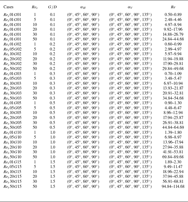


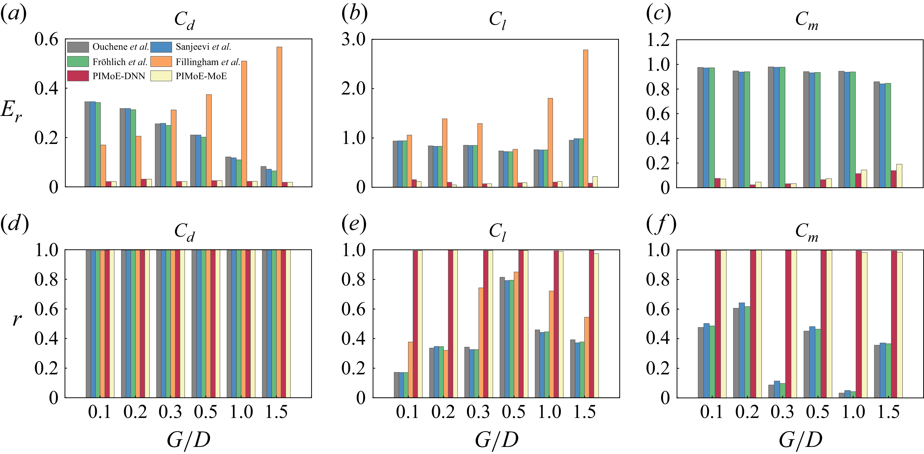


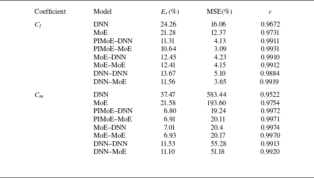


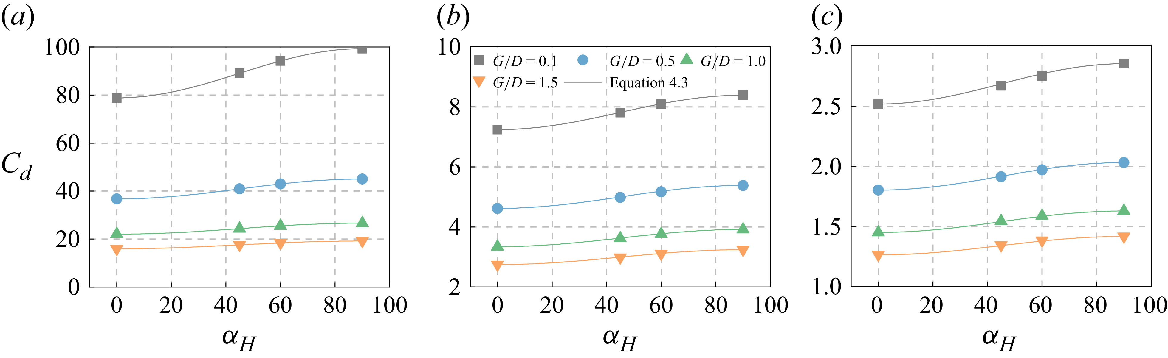


 Open access