







1. Introduction
Simple structural elements such as beams or elastic filaments interacting with fluid flows have been studied largely because of their massive use in many technological applications, and importance in environmental and biological flows. For instance, suspension of fibres is often employed in low-Reynolds-number flows for studying biological transport processes such as microorganisms swimming (Lauga & Powers Reference Lauga and Powers2009), while in turbulent flows fibres have been adopted, usually mixed with polymers (Lee, Vaseleski & Metzner Reference Lee, Vaseleski and Metzner1974), for drag reduction purposes (Paschkewitz et al. Reference Paschkewitz, Dubief, Dimitropoulos, Shaqfeh and Moin2004). Recently, suspended fibres have been studied in turbulent flows to exploit their usage as a proxy of turbulence statistics, in particular using an end-to-end length of the fibre as reference length scale for quantifying two-point statistics (Rosti et al. Reference Rosti, Banaei, Brandt and Mazzino2018a, Reference Rosti, Olivieri, Banaei, Brandt and Mazzino2020; Olivieri, Mazzino & Rosti Reference Olivieri, Mazzino and Rosti2021), with the development of the novel technique of fibre tracking velocimetry (Brizzolara et al. Reference Brizzolara, Rosti, Olivieri, Brandt, Holzner and Mazzino2021).
Surfaces of anchored filamentous layers exposed to fluid flows are found commonly in nature, paving the way for novel bio-inspired technologies (Alvarado et al. Reference Alvarado, Comtet, De Langre and Hosoi2017). At microscales, ciliated walls and flagella are found commonly in living organs (e.g. microvilli, cilia in the bronchial epithelium, papillae of tongues, cilia of kidney cells), participating in a number of physiological processes such as locomotion, digestion, circulation, respiration and reproduction (Lodish, Berk & Kaiser Reference Lodish, Berk and Kaiser2007). Enlarging the range of scales considered, the interaction of surfaces covered by complex texture with surrounding fluid flows is adopted in nature for a wide variety of tasks, such as decreasing skin friction drag (e.g. seal fur, see Itoh et al. Reference Itoh, Iguchi, Yokota, Akino, Hino and Kubo2006) and control of flight aerodynamics (e.g. birds’ feathers, see Brücker & Weidner Reference Brücker and Weidner2014). An active branch of research concerns the interaction of vegetative plants immersed in the atmospheric environment (terrestrial canopies) and water (aquatic canopies) (Raupach & Thom Reference Raupach and Thom1981; Finnigan Reference Finnigan2000; Nepf Reference Nepf2012). In terrestrial canopies, the exchange of mass, heat and momentum between the canopy layer and the environmental surroundings regulates the micro-climate, providing, for instance, plants with carbon dioxide for photosynthesis (Raupach & Thom Reference Raupach and Thom1981); in an aquatic environment, instead, vegetation contributes significantly to creating habitats for microorganisms by influencing the nutrient transport and deposition, by improving water quality (especially useful in the treating of grey water) and by regulating the solar light uptake (Mars, Mathew & Ho Reference Mars, Mathew and Ho1999; Ghisalberti & Nepf Reference Ghisalberti and Nepf2002; Luhar, Rominger & Nepf Reference Luhar, Rominger and Nepf2008; Wilcock et al. Reference Wilcock, Champion, Nagels and Croker1999).
The mentioned examples vary widely, with mechanical properties depending highly on the tasks that the filamentous layer has to address. Therefore, a large variety of parameters must be accounted for to characterize correctly the specific behaviour of each canopy configuration immersed in a fluid flow. These parameters span from purely geometrical properties (e.g. aspect ratio, size and shape of the stems, level of submersion, angle of inclination of the root of the stems) to mechanical aspects (e.g. flexibility, density ratio, active or passive motions); including them all in a parametric study makes the analysis of canopy flows a very challenging topic. In previous investigations, researchers focused on finding a reduced set of parameters to characterize common behaviours that helped to identify a standard classification of the flows. The geometric argument has been debated thoroughly, and in the bulk of the literature, the level of submersion – defined as the ratio between the flow depth  $H$ and the canopy height $h$ – and the solidity – a parameter that associates the frontal area of the canopy layer to the area of the canopy bed – have been adopted extensively to classify canopy flows (see the reviews Nepf Reference Nepf2012; Brunet Reference Brunet2020). In particular, the former is used to distinguish emergent canopies ( $H/h\le 1$), where the resulting flow is dominated by the balance between the drag offered by the canopy elements and the driving pressure gradient, with turbulence dominated by the vortices shed by the stems of canopy (Nepf & Vivoni Reference Nepf and Vivoni2000), from submerged canopies ( $H/h > 1$), where the flow is more complex due to the several scales involved, e.g. the diameter of the stems $d$, the height of the canopy $h$, the average distance between the stems $\Delta S$, and the size of the domain $H$, to mention a few of them (Nepf Reference Nepf2012, see also figure 1). In the literature, some of the parameters mentioned above have been merged to define the so-called solidity,
 \begin{equation} \lambda=\int_0^{h} \,d(y)/\Delta S^{2}\, \mathrm{d}y, \end{equation}
an indicator of the density of the canopy that has been used to classify the submerged canopy flows into regimes that range from sparse to dense based on a threshold value (i.e.  $\lambda _{t} \approx 0.1$) defined by means of experimental evidence (Poggi et al. Reference Poggi, Porporato, Ridolfi, Albertson and Katul2004; Nepf Reference Nepf2012). In particular, it has been accepted widely that for values much smaller than $\lambda _{t}$, the flow velocity above and within the canopy shows a behaviour comparable to flows bounded by a solid wall covered by roughness elements (sparse regime); conversely, the form drag offered by the stems becomes dominant (dense regime) for large values of $\lambda$, and the mean velocity profile shows the typical two inflection points caused by the drag discontinuity at the tip of the canopy (upper inflection point, located at the edge of the canopy layer) and by the merging of the inflected profile below the canopy tip and the boundary layer developed in the proximity of the wall (lower inflection point). In this regime, a stratified model with three separated layers of the flow has been proposed (Belcher, Jerram & Hunt Reference Belcher, Jerram and Hunt2003; Poggi et al. Reference Poggi, Porporato, Ridolfi, Albertson and Katul2004; Nezu & Sanjou Reference Nezu and Sanjou2008). The layers can be identified as follows. Above the upper inflection point, $y/h > 1$, an outer region with a behaviour typical of a boundary layer over a rough wall can be identified (Raupach, Finnigan & Brunet Reference Raupach, Finnigan and Brunet1996; Finnigan Reference Finnigan2000). In the canopy region, instead, $y/h \ll 1$, the flow is assumed to be characterized by the wakes shed by the canopy elements, similarly to an emergent canopy configuration. Finally, in the region in between, the flow is assumed to be dominated by a mixing layer of constant thickness (Ghisalberti & Nepf Reference Ghisalberti and Nepf2004).
Geometrical parameters governing a canopy flow (Nepf Reference Nepf2012).

Most of the past studies were of experimental nature that are of difficult realization and can hardly display, especially within the canopy, a complete portrait of the mechanisms that characterize the mutual interaction between the stratified layers, due to the natural impedance enforced by the presence of the canopy layer itself. With increasing computational power and the introduction of advanced techniques that enabled a full implementation of the canopy layer, new high-fidelity numerical studies have surged in the last few years (Sharma & García-Mayoral Reference Sharma and García-Mayoral2018; Monti, Omidyeganeh & Pinelli Reference Monti, Omidyeganeh and Pinelli2019; Monti et al. Reference Monti, Omidyeganeh, Eckhardt and Pinelli2020; Tschisgale et al. Reference Tschisgale, Löhrer, Meller and Fröhlich2021). In particular, Monti et al. (Reference Monti, Omidyeganeh, Eckhardt and Pinelli2020) carried out a set of high-fidelity simulations – wall-resolved large-eddy simulation (LES) – of open-channel flows bounded by a rigid wall-normally mounted canopy simulated via a state-of-the-art immersed boundary method. In their work, a parametric study has been investigated, choosing as free parameter the height of the canopy layer (thus setting implicitly the solidity  $\lambda$). The different heights analysed have been selected to span canopy flows from a marginally sparse regime to a dense one. With this study, a detailed characterization of the canopy regimes has been given, providing the literature with new insights on the structures populating the inner and outer regions. To better identify the transition from the sparse regime to a dense regime, the authors presented a new criterion built on a simple physical model that establishes if the largest vortex of the outer region could reach the bed, based on the geometrical properties of the filamentous layer; with this model, a new threshold value of solidity was found as lower bound for the dense regime, i.e. $\lambda _{t}\approx 0.15$. The model was built upon the geometrical parameters characterizing the solidity, but the latter may be a questionable parameter for classifying canopy flows. For instance, simply considering rigid cylindrical stems with uniform length and diameter, inclined with opposite angles $\theta$ in the direction of the flow ( $\theta >0$ flow with the grain, $\theta <0$ flow against the grain, Alvarado et al. Reference Alvarado, Comtet, De Langre and Hosoi2017), the solidity value remains unchanged, while a very different behaviour of the flow can be expected. This consideration may be extended to a more general flexible canopy. Therefore, using $\lambda$ alone to classify the flow may not be an adequate choice.
To address this uncertainty, in this work we analyse a set of rigid canopies assembled with cylindrical stems, inclined at a certain angle  $\theta$ in the streamwise direction. The angle of inclination is varied systematically from a wall-normal condition $\theta =0^{\circ }$ to a condition that matches the lowest solidity value analysed in Monti et al. (Reference Monti, Omidyeganeh, Eckhardt and Pinelli2020), i.e. $\lambda =0.07$, resulting in an inclination $\theta =\pm 78.5^{\circ }$. The whole analysis will be carried out by means of highly-resolved LES, with the canopy layer simulated with a stem-by-stem approach implemented via an extensively validated immersed boundary method.
The paper is organized as follows. Section 2 describes the numerical method used to perform the simulations. Section 3 describes the obtained results that combine statistical results with instantaneous realizations. Finally, § 4 outlines the most important conclusions of the present work.
2. The numerical method
Turbulent flows over rigid canopies have been simulated by means of a numerical solver (SUSA, Omidyeganeh & Piomelli Reference Omidyeganeh and Piomelli2013) that solves the incompressible Navier–Stokes equations. In particular, we adopted an LES approach, where the velocity and pressure field obtained are a result of a high-pass filtering operation. In a Cartesian frame of reference, where  $x_1$, $x_2$ and $x_3$ (sometimes also referred to as $x$,
$x$,  $y$ and $z$) are adopted to identify the streamwise, wall-normal and spanwise directions, with $u_1$, $u_2$ and $u_3$ the corresponding velocity components (or $u$,
$u$,  $v$ and $w$), the dimensionless incompressible LES equations for the resolved fields $\bar {u}$ and $\bar {p}$ read as
 \begin{equation} \frac{\partial \bar{u}_i}{\partial t} + \bar{u}_j\,\frac{\partial \bar{u}_i}{\partial x_j} ={-} \frac{\partial \bar{P}}{\partial x_i} + \frac{1}{Re_b}\,\frac{\partial^{2} \bar{u}_i}{\partial x_j\, \partial x_j} + \frac{\partial \tau_{ij}}{\partial x_j} + f_i, \frac{\partial \bar{u}_i}{\partial x_i} = 0. \end{equation}
In (2.1),  $Re_b=U_b H/\nu$ is the Reynolds number based on the bulk velocity $U_b$, the open channel height $H$, and the kinematic viscosity $\nu$, while $\tau _{ij}=\overline {u_i u_j}-\bar {u}_i \bar {u}_j$ is the subgrid Reynolds stress tensor (Leonard Reference Leonard1975). (From now on, the overbar will be dropped to simplify the notation.) To close the equations, an eddy viscosity approach used to model the unresolved subgrid stress tensor was adopted. In particular, we employ the integral length scale approximation (ILSA) proposed by Piomelli, Rouhi & Geurts (Reference Piomelli, Rouhi and Geurts2015) (see also Rouhi, Piomelli & Geurts Reference Rouhi, Piomelli and Geurts2016). The incompressible LES equations (2.1) are discretized spatially with a second-order-accurate, cell-centred finite volume method. Pressure and velocity are evaluated at the centres of the cells in a collocated grid fashion, and to avoid the appearance of spurious pressure oscillations, the corrective approach proposed by Rhie & Chow (Reference Rhie and Chow1983) has been adopted. To advance the equations in time, we adopted a second-order semi-implicit fractional-step method (Kim & Moin Reference Kim and Moin1985), where the implicit Crank–Nicolson scheme is implemented for the wall-normal diffusive terms and an explicit Adams–Bashforth scheme is applied to all other terms. The Poisson equation for the pressure, required to enforce the solenoidal condition of the velocity field, is decoupled into a series of two-dimensional Helmholtz equations in the wavenumber space, applying a fast Fourier transform along the spanwise direction, and solved through the iterative biconjugate gradient stabilized method with an algebraic multigrid preconditioner (boomerAMG, see Yang et al. Reference Yang2002). The code is parallelized using the domain decomposition technique.
The canopy is implemented as a set of stems represented as rigid solid slender cylindrical rods of finite cross-sectional area, mounted in parallel onto the impermeable bottom wall with an angle of inclination that constitutes a free parameter in this work. The enforcement of the boundary conditions on the surface of the rigid cylinders (zero velocity) is obtained by means of an immersed boundary method (IBM) that deals with the presence of the rods by using a set of nodes (Lagrangian nodes) distributed along the length of each canopy element that do not necessarily conform with the fluid grid. More specifically, at every time step, the employed IBM (Pinelli et al. Reference Pinelli, Naqavi, Piomelli and Favier2010) associates to every Lagrangian node a set of distributed body forces whose intensity can be computed by enforcing the no-slip condition on the nodes. The distributed set of body forces is defined on a compact support centred on each node of the Lagrangian mesh used to define the stems. The size of the support is related to the local grid size and defines the hydrodynamic thickness of the filament. An appropriate study that investigates the adequate number of Lagrangian nodes to be used to replicate satisfactorily the flow around a set of filaments has been done previously by Monti et al. (Reference Monti, Omidyeganeh and Pinelli2019), who compared the outcomes obtained with the current methodology to the results from a simulation with an immersed boundary method that imposes directly the correct boundary conditions on the surface of the filaments (Fadlun et al. Reference Fadlun, Verzicco, Orlandi and Mohd-Yusof2000). From that study, we concluded that a Lagrangian lattice with four points per cross-section was enough to reproduce adequately the physics of the problem. Therefore, we set the diameter of the filaments indirectly to be around  $2.2 \Delta x$ (Monti et al. Reference Monti, Omidyeganeh and Pinelli2019), or $2.2 \Delta z$, since the mesh spacing is the same in the $x$ and $z$ directions.
Finally, to prove the appropriateness of the method, we report here the results of the validation campaign (Monti et al. Reference Monti, Omidyeganeh and Pinelli2019), where we compare directly an appositely set-up simulation using the experimental results (R31) by Shimizu et al. (Reference Shimizu, Tsujimoto, Nakagawa and Kitamura1991), with wall-normally mounted rigid filaments of height  $h/H=0.65$, solidity $\lambda =0.41$, and bulk Reynolds number $Re_b=7070$. The comparison between the velocity profile and the Reynolds shear stress obtained is shown in figure 2, with pretty good agreement of the results. The parameters of the simulation used for the validation case are provided in table 1 together with the corresponding experimental values (Shimizu et al. Reference Shimizu, Tsujimoto, Nakagawa and Kitamura1991). Note that the viscous units used to compute the friction Reynolds numbers listed in table 1 (and therefore the resolution parameters) are based on the total shear stress at the solid wall ( $in$ subscript) and at the canopy tip ( $out$ subscript), with $\Delta y^{+}_{w,in}$ and $\Delta y^{+}_{h,out}$ indicating the resolutions of the first computational cell at the wall and at the canopy tip, respectively.
Validation results (for more details, see Monti et al. Reference Monti, Omidyeganeh and Pinelli2019). (a) Mean velocity profile and (b) Reynolds shear stress distribution from our simulations (solid line) compared with the experimental values R31 by (Shimizu et al. Reference Shimizu, Tsujimoto, Nakagawa and Kitamura1991) (dotted curve). The dashed line shows the location of the canopy tip at  $y=h$.

Validation case parameters.

As we mentioned above, the stems are distributed on the bottom wall. In particular, we have subdivided the latter in a Cartesian lattice of uniform squares of area  $\Delta S^{2}$, with the filaments within each tile positioned randomly. The use of a random assignment on each tile prevents preferential flow channelling effects. A sketch of the distribution of the stems on the channel bottom wall is shown in figure 3.
(a) Filaments distribution on the bottom of the computational domain. The red box is zoomed out in (b), where the random allocation of each filament within a  $\Delta S \times \Delta S$ tile is highlighted.

In order to assess the general usefulness of the solidity (defined in (1.1)) as critical parameter in the framework of canopy flows, we adjust the size of the tile and the angle of inclination of the stems (given the length of the filaments) to match solidity values that span from the quasi-sparse regime to the dense one (Nepf Reference Nepf2012; Brunet Reference Brunet2020). In particular, for stems with a uniform cross-sectional circular area of diameter  $d$, the solidity simply reads as
 \begin{equation} \lambda=\frac{dl_\perp}{\Delta S^{2}}, \end{equation}
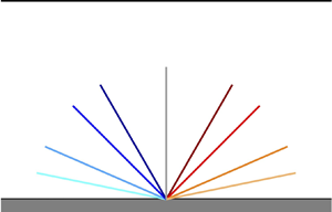
where  $l_\perp = l\cos (\theta )$ is the projection of the length of the filament $l$ along the wall-normal direction, defining the height of the canopy layer $l_\perp =h$, with $\theta$ being the angle of inclination positive in the clockwise direction counted from the wall-normal direction (see figure 4; note that the colour scheme used to indicate the different inclinations will be kept for the remainder of the paper). In this work, to vary the value of the solidity, we fix the size of the tile $\Delta S$ (fixing the number of filaments in the streamwise and spanwise directions to $nf_x\times nf_z$), the diameter and the length of the filaments, and we vary the value of the inclination $\theta$. In particular, we chose eight angles, ranging symmetrically from $\theta =\pm 78.5^{\circ }$ around $\theta =0$ (i.e $\lambda =0.07,0.14,0.25,0.30,0.35$). The nine cases share the same computational box of size $L_x/H = 2{\rm \pi}$, $L_y/H = 1$ and $L_z/H = 3{\rm \pi} /2$, similar to other works (Bailey & Stoll Reference Bailey and Stoll2013; Monti et al. Reference Monti, Omidyeganeh, Eckhardt and Pinelli2020).
Sketch of the inclined canopy cases considered. The colour scheme refers to the angle of inclination selected and will be used for the whole paper. From left to right, in clockwise order,  $\theta =-78.5^{\circ }$, $-66.5^{\circ }$, $-45^{\circ }$, $-30^{\circ }$, $0^{\circ }$, $30^{\circ }$, $45^{\circ }$, $66.5^{\circ }$, $78.5^{\circ }$.

The numerical domain is set to be periodic in both the streamwise (i.e.  $x$) and spanwise (i.e. $z$) directions; at the bottom wall, a no-slip boundary condition is imposed, while at the top surface, a free-slip condition is set to mimic an open-channel free surface. The Cartesian computational lattice is distributed uniformly in the horizontal directions, while a stretched distribution (with ratio between neighbouring cells kept below $4\,\%$) is adopted in the wall-normal direction. The latter, in particular, is built using two tangent-hyperbolic functions that concentrate the nodes in the regions where higher shears are expected, i.e. at the edge of the canopy layer and close to the solid wall. The total number of nodes is equal to $N_x=576$ and $N_z=432$, while $N_y\in [230,300]$, with the lower and upper cases set for the most inclined and wall-normally mounted cases, respectively. The number of nodes has been selected such that the spacings in wall units satisfy the standard values suggested for wall-bounded flows (Kim, Moin & Moser Reference Kim, Moin and Moser1987); the wall units are estimated using the maximum value of the viscous length scale based on the local shear stress (further explanations on the evaluation of the local viscous scales are provided in the next section and in Monti et al. Reference Monti, Omidyeganeh and Pinelli2019). Note that the maximum value of the local shear stress is obtained at the canopy edge; therefore, the wall-normal grid spacing in wall units considered is evaluated considering the value at the tip of the canopy. Finally, to drive the flow, a uniform pressure gradient is applied in the streamwise direction. In particular, at each time step, the mean streamwise pressure gradient is adjusted to fix the flow rate to a constant value corresponding to bulk Reynolds number $Re_b=U_b\,H/\nu =6000$, a value close to those available already in the literature (Shimizu et al. Reference Shimizu, Tsujimoto, Nakagawa and Kitamura1991; Bailey & Stoll Reference Bailey and Stoll2013). The detailed parameters of the simulations are listed in table 2.
Set of parameters for the inclined canopies. From left to right: angle of inclination; length of the filaments; wall-normal projection of the filaments (height of the canopy layer  $l_\perp =h$); average spacing between the filaments; solidity; numbers of filaments in the streamwise and spanwise directions; number of nodes of the computational mesh in the wall-normal direction; friction Reynolds number $Re_\tau =u_\tau H/\nu$, where $u_\tau$ is computed evaluating the value of the total shear stress at the canopy tip; resolution of the computational domain in wall units, where $\Delta y_h^{+}$ is evaluated in the region of maximum shear, i.e. at the edge of the canopy.

For the sake of completeness, we point out that the formulation of the problem used in this work can be considered as a coarse direct numerical simulation (DNS) in the outer portion of the flow that becomes progressively highly resolved as the canopy is approached. In the outer flow region, the subgrid stress contribution plays the role of only a very mild and stabilizing numerical dissipation. Indeed, the ratio between the total and subgrid energies averaged in time and in the two homogeneous directions, shown in figure 5(a) (dashed line) along the channel height, is always below  $10^{-5}$. Concerning the subgrid stress activity along the streamwise direction (dominant in a shear-driven flow), the LES model always contributes a value far below $0.1$, excluding the region in the proximity of the wall (not so relevant for canopy flows), as shown by the ratio between the subgrid shear stress and the total one (Rouhi et al. Reference Rouhi, Piomelli and Geurts2016) averaged in time and in the two homogeneous directions in figure 5(a) (solid line). These a posteriori checks allowed us to avoid introducing any particular treatment for the coupling between the LES and the IBM. A further indication that the LES filter operates at the end of the turbulence cascade is provided in figure 5(b), showing that the ratio between the time- and space-averaged eddy viscosity and the physical one is always of order unity or less throughout the whole channel. Note that the curves shown in figure 5 refer to the case $\theta =-30^{\circ }$; the other scenarios show similar trends and, as such, are not reported for the sake of clarity.
(a) Dashed line: ratio between the subgrid energy and the total fluctuating energy along the wall-normal direction. Solid line: ratio between the subgrid shear stress and the total fluctuating shear stress along the wall-normal direction. (b) Ratio between the eddy viscosity and the physical viscosity along the wall-normal direction. In both panels, the superscript  $sgs$ indicates the subgrid stress tensor (eddy viscosity in (b)) component, while in (a), the superscript $tot$ refers to the total part of the stress tensor, i.e. the summation of the resolved and subgrid parts. The reference case chosen is $\theta =-30^{\circ }$, consistent with the colour map in figure 4.

3. Results
The results collected in this section present the flow statistics characterizing the flow and illustrate the emergence of various coherent structures related to the various regimes encountered (see table 2). In particular, the section is structured as follows: the first part deals with the mean velocity profiles, analysing the location of the inflection points and the location of the (virtual) origin of the boundary layer developed in the outer part of the flow; in the second part, we introduce the higher-order statistics and describe extensively the turbulent coherent structures that characterize the flow.
Note that all the quantities shown in this section will be reported in a non-dimensional form.
3.1. Canopy properties
First, we analyse the effect of the canopy inclination on the mean velocity profile; the aim is to show that positive and negative inclination angles  $\theta$ have very different impacts on the bulk statistics of the flow, thus proving that a simple prediction of the canopy flow regimes based on the solidity parameter $\lambda$ is not always meaningful. Figure 6 shows the mean velocity profiles close to the canopy tips (marked by the symbol $\blacksquare$), with figure 6(a) showing the canopies inclined with the grain, $\theta >0$, and figure 6(b) showing the cases inclined against the grain, $\theta <0$. All the cases considered show the typical convex region of the velocity profile within the canopy layer, confined by two inflection points that arise from the discontinuity of the drag at the canopy edge as a consequence of the sudden end of the stems (upper inflection point), and as a result of the merging of the boundary layer in the proximity of the wall and the convex region (lower inflection point, $y_{lip}$). A higher or lower curvature of the convex region depends on the penetration level of the flow above the canopy. Since figure 6 shows qualitatively that the mean velocity profile within the canopy (i.e. below the marker $\blacksquare$) has a milder convexity when the filaments are inclined against the grain ( $\theta <0$), we expect to find a higher penetration of the outer flow in these scenarios. To verify this, we analyse the locations of the most significant points of the mean velocity profile (the markers in figure 6), i.e. the already mentioned two inflection points enclosing the convex region, and the virtual origin for the outer flow, $y_{vor}$, defined as the location of the effective wall for the outer boundary layer, that can be determined by enforcing the mean outer flow to take on a canonical logarithmic shape, as shown by Monti et al. (Reference Monti, Omidyeganeh and Pinelli2019). In particular, we focus on the locations of the virtual origin and the inner inflection point in figures 7(a) and 7(b), respectively. While the location of the inner inflection point differs only slightly between the positive and negative values of $\theta$, the location of the virtual origin reveals clearly the large difference of the penetration of the outer flow in the two opposite configuration. Figure 7(a) shows quantitatively the intuitive effect of the inclination: the negative angles promote the penetration of the outer flow structures within the canopy, while the positive ones shelter the layer from the large vortices.
Mean velocity profiles for the canopies inclined with the grain (a) and against the grain (b). The small inset in each plot shows an enlarged view that visualizes the mean velocity profiles along the whole channel depth. The three symbols indicate: the location of the first inflection point ( $\bigstar$), the location of the virtual origin ( $\bullet$), and the location of the canopy tip, i.e. the second inflection point ( $\blacksquare$).

(a) Hysteresis of the location of the virtual origin with the canopy inclination angle, represented using the wall-normal projection of the canopy layer. (b) Hysteresis of the location of the inner inflection point with the canopy inclination angle, represented using the wall-normal projection of the canopy layer. The symbols  $\blacktriangleright$ refer to the canopies inclined with the grain, while the symbols $\blacktriangleleft$ refer to the canopies inclined against the grain. The symbol $\blacklozenge$ refers to the wall-normally mounted canopy. The colour scheme is the one used in table 2.

To conclude the analysis on the features of the mean velocity profile, we consider the relative location of the virtual origin and the inner inflection point. According to Monti et al. (Reference Monti, Omidyeganeh, Eckhardt and Pinelli2020), these quantities define the transition from a quasi-sparse canopy flow to a dense one, since the location of the lower inflection point marks the end of the boundary layer close to the canopy bed, and the virtual origin marks a lower limit for the outer flow; therefore, a crossing between these two points means that the two regions overlap and the transitional to sparse scenario described by Nepf (Reference Nepf2012) appears. Figure 8 reports the trends of the locations of the virtual origins (solid lines) and the inner inflection points (dashed lines) compared to the data obtained for the wall-normally mounted canopies (black lines) taken from Monti et al. (Reference Monti, Omidyeganeh, Eckhardt and Pinelli2020). In particular, the figure shows that when the filaments are inclined positively (red lines in figure 8a), the intersection between the two curves moves closer to the wall than when wall-normally mounted, meaning that a dense-like regime develops even for very low values of solidity. On the contrary, when the filaments have a negative inclination (blue lines in figure 8b), the intersection point is shifted towards the canopy tip, in a sparse-like canopy fashion. Therefore, two canopies inclined by an opposite angle  $\theta$ but having the same solidity $\lambda$ may behave in a completely different manner. This is a clear indication that a classification of the canopy regimes based on the solidity alone – as has been done largely in the literature, i.e. $\lambda > 0.1$ (Poggi et al. Reference Poggi, Porporato, Ridolfi, Albertson and Katul2004; Nepf Reference Nepf2012; Brunet Reference Brunet2020) – can actually be misleading.
Locations of the inner inflection points (empty symbols) and the virtual origins (filled symbols) along the wall-normal projection of the canopy. The abscissa indicates the canopy case considered based on the wall-normal canopy projection  $l_\bot$. The lines represent the polynomial fits passing by the virtual origin (solid lines) and the inner inflection points (dashed lines). The red lines (a) refer to the canopies inclined with the grain, while the blue lines (b) refer to the ones inclined against the grain. The black lines indicate the wall-normally mounted canopies data from Monti et al. (Reference Monti, Omidyeganeh, Eckhardt and Pinelli2020). The crossing point of two lines of the same colour indicates the transition from a quasi-sparse regime to a dense regime.

The shape of the mean velocity profile described above is caused by the resistance that the flow encounters when flowing through the stems of the canopy layer. The drag exerted by the canopy can be quantified by the mean pressure gradient needed to move the flow. Figure 9(a) shows the mean pressure gradient as a function of the wall-normal projection of the canopy layer  $l_\bot$. As reference, the values of the wall-normally mounted canopies studied in Monti et al. (Reference Monti, Omidyeganeh, Eckhardt and Pinelli2020) have been added to the graph (diamonds, greyscale). The figure shows that a positive inclination always reduces the drag compared to negatively inclined canopies, suggesting that the sheltering effect is beneficial in these terms. Figure 9(a) shows also that for short canopy layers, i.e. $l_\bot /H < 0.15$, the inclination (negative and positive) is also beneficial compared to the wall-normally mounted canopies having the same frontal area (black solid line). However, when increasing $l_\bot /H$, only the cases with negative $\theta$ result in drag increasing (blue solid line) in figure 9(a). To corroborate this result, the drag coefficient provided by the canopy layer,
 \begin{equation} C_D = \dfrac{2 \mathbb{D}}{\rho U_b^{2} H L_z}, \end{equation}
is shown in the inset of figure 9(a). In (3.1),  $\mathbb {D}$ is the integral drag force provided by the whole canopy, $\rho$ is the density of the fluid, $U_b$ is the bulk velocity, and $H\times L_z$ is the frontal area of the whole computational domain. Note that the trend of the drag coefficient reflects the trend of the pressure gradient since the former is the main contribution to the latter in a canopy flow. These behaviours are due mainly to the type of turbulent structures forming and living within the canopy layer, as will be shown later in the paper.
Non-dimensional mean pressure gradient versus (a) the height of the canopy layer  $l_\perp$, and (b) the roughness function $\Delta U^{+}_{out}$ related to the outer boundary layer developed starting from the location of the virtual origin, rescaled by the fraction of the domain occupied by the latter. The inset in (a) shows the drag coefficient $C_D$ provided by the canopies analysed in this work versus the height of the canopy layer $l_\perp$. The shapes and colours of the symbols are as adopted in figure 7. The greyscale diamonds refer to the cases analysed in Monti et al. (Reference Monti, Omidyeganeh, Eckhardt and Pinelli2020).

Figure 9(b) shows that the pressure gradient is related strictly to the level of penetration of the outer flow within the canopy layer and the resistance felt by the outer flow caused by the tips of the canopy stems that can be thought of as elements of a distributed roughness. Indeed, the figure shows an almost exponential-law behaviour, independently of the canopy configuration, when the friction function  $\Delta U^{+}_{out}$ is normalized by the percentage of the open-channel domain occupied by the outer layer. The friction function is an offset added to the logarithmic law of the mean velocity in a turbulent boundary layer over a smooth wall to characterize the presence of roughness (Jiménez Reference Jiménez2004), and for the outer flow in a canopy, it can be defined as in Monti et al. (Reference Monti, Omidyeganeh and Pinelli2019),
 \begin{equation} \Delta U^{+}_{out} = \kappa^{{-}1} \log{\dfrac{(y-y_{vor})u_{\tau,out}}{\nu}} + B - U^{+}_{out}, \quad \quad \text{for} \ y > y_{vor}, \end{equation}
where the first part of the right-hand side is the logarithmic law for a boundary layer over a smooth wall located at the virtual origin  $y_{vor}$, and the second part is the mean velocity profile found in the outer flow in a canopy normalized by the friction velocity $u_{\tau,out}$ computed at the virtual origin; in the equation, $\kappa =0.41$ is the Kármán constant, $\nu$ is the kinematic viscosity, and $B=5.5$ is the additive constant for smooth walls. The mean velocity profiles obtained from (3.2) are shown in figure 10, together with the inner part of the profile normalized with the inner viscous units for the sake of completeness. Relation (3.2) links together the pressure gradient and the outer flow quantities only, but the former is computed by considering the whole drag offered by the canopy, therefore the relation links implicitly the quantities of the outer and inner layers. The connection between the regions that characterize the canopy flows will be clarified in the next subsection, where a detailed description of the coherent structures will be given.
Mean velocity profiles normalized using the viscous quantities defined in the inner layer, i.e. the friction velocity  $u_\tau ^{*}=u_{\tau,in}$ computed at the bottom wall $y_w^{*}=0$, and the viscous quantities defined in the outer layer, i.e. the friction velocity $u_\tau ^{*}=u_{\tau,out}$ computed at the virtual origin $y_w^{*}=y_{vor}$. The abscissa represents the wall-normal coordinate rescaled with the inner or outer wall units, considering an origin located either on the canopy bed or at the virtual origin $y_{vor}$. The profiles in (a) refer to the canopies inclined with the grain, while the profiles in (b) refer to the ones inclined against the grain. The grey lines indicate the wall-normally mounted canopies with $h/H=0.25$ from Monti et al. (Reference Monti, Omidyeganeh, Eckhardt and Pinelli2020). The shapes and colours of the symbols are as adopted in figure 7.

3.2. Canopy structures
Before describing the turbulent coherent structures that populate the canopy flows, we discuss the mean distributions of the velocity fluctuations since they contain important information concerning the turbulent properties of the flow. Figure 11 shows a comparison of the r.m.s. of the velocity fluctuations between the positively (figures 11a–c) and negatively (figures 11d–f) inclined canopies, with the profiles of the wall-normally mounted canopy shown as reference (grey lines). The velocity fluctuations are normalized with the external friction velocity  $u_{\tau,out}$, obtained using the total stress at the virtual origin. The curves collapse in the region outside the canopy, confirming once more the behaviour of the outer flow as a boundary layer over a virtual rough wall (Monti et al. Reference Monti, Omidyeganeh and Pinelli2019, Reference Monti, Omidyeganeh, Eckhardt and Pinelli2020), while inside the canopy layer, the comparison becomes more challenging because of the change of the frontal area with the inclination. To overcome this problem, we introduce a velocity scale based on the combination of the imposed pressure gradient and the drag exerted by the filaments:
 \begin{equation} u_{\tau,l}(y) = \sqrt{\frac{\mu d_y \, \langle u \rangle - \rho \, \langle u'v' \rangle}{\rho \,(1-y/H)}}. \end{equation}
In the above,  $\mu d_y\,\langle u\rangle$ is the viscous shear stress, and $\rho \,\langle u'v' \rangle$ is the turbulent shear stress. For more details on the explicit derivation of (3.3), the reader is referred to Monti et al. (Reference Monti, Omidyeganeh and Pinelli2019). When normalizing the r.m.s. of the velocity fluctuations with $u_{\tau,l}$, a better collapse is achieved within the canopy layer, as shown in figure 12. In particular, we obtain a set of profiles comparable to the ones corresponding to an open channel flow over a smooth wall. We note that the maximum of the streamwise velocity fluctuations (figures 12a,d) decreases as the angle of inclination for $\theta >0$ (figures 12a–c) decreases, with the wall-normally mounted canopy inverting the trend (grey line). The opposite is true for the cases $\theta <0$ (figures 12d–f), where the peak of $u'_{rms}$ increases by decreasing the inclination angle, dropping when $\theta =0$ (grey line). The peak of the streamwise velocity fluctuations close to the wall suggests the presence of coherent structures in that region, similar to streaks. However, the presence of the stems makes the development of classic streaks and the typical wall cycle (Jiménez & Pinelli Reference Jiménez and Pinelli1999) unlikely, so the peak of $u'_{rms}$ is more likely related to the high-speed and low-speed regions evolving between the stems, similarly to a biperiodic flow past a set of cylinders. Concerning the wall-normal fluctuations $v'_{rms}$ within the canopy, as already observed by Monti et al. (Reference Monti, Omidyeganeh, Eckhardt and Pinelli2020), the normalized distribution does not differ qualitatively from the one observed in an open-channel flow over a smooth wall, suggesting that the filtering effect of the stems acts only along the homogeneous directions. Although the observation is still valid in the context of inclined canopies, we must point out that the intensity of $v'_{rms}$ within the canopy layer tends to decrease monotonically as the inclination $|\theta |$ increases, with the negatively inclined canopies having a larger value, as expected, since the penetration of the outer flow is facilitated. Finally, the spanwise velocity fluctuations show the most interesting behaviour, with a large peak related to the deviation of the streaky structures (peak of $u'_{rms}$) caused by the presence of the stems. The trend of its maximum is similar to that of $v'_{rms}$, suggesting that the intensity of spanwise velocity structures close to the wall is dominated by the penetration of the large outer structures for taller canopies (i.e. lower $|\theta |$), while for shorter canopies (i.e. higher $|\theta |$), the outer and inner flows are mixed, with the former dictating the coherence near the bed.
Profiles of the r.m.s. of the velocity fluctuations versus the wall-normal coordinate  $y/H$. (a–c) Distributions of the canopies inclined with the grain. (d–f) Distributions of the canopies inclined against the grain. (a,d) Streamwise component, (b,e) wall-normal component, and (c, f) spanwise component. The distributions are normalized with the friction velocity computed at the virtual origin, $u_{\tau,out}$. Colours as in table 2.

Profiles of the r.m.s. of the velocity fluctuations versus the wall-normal coordinate  $y/H$. (a–c) Distributions of the canopies inclined with the grain. (d–f) Distributions of the canopies inclined against the grain. (a,d) Streamwise component, (b,e) wall-normal component, and (c, f) spanwise component. The distributions are normalized with the local friction velocity defined in (3.3). Colours as in table 2.

Further insight into the structures populating the flow can be obtained by analysing the spectral energy content of the fluctuations of the velocity components. We start by looking at the structures of the wall-normally mounted canopy flow to describe the phenomenology that bonds together the outer and inner flows when the scale separation introduced by the tall stems is expected (dense regimes). In figure 13, we present the one-dimensional premultiplied spectra of the velocity fluctuations and the magnitude of the one-dimensional premultiplied co-spectra of the Reynolds shear stress, as a function of the distance from the wall, organized in a  $2\times 4$ matrix of panels, where each column of the matrix shows, in order, the streamwise, wall-normal and spanwise components of the velocity fluctuations, and the fourth column the magnitude of the co-spectra of the Reynolds shear stress. In figure 13(a–d), the quantities are plotted as a function of the streamwise wavelength, while in figure 13(e–h) they are plotted as a function of the spanwise wavelength.
Case  $\theta =0^{\circ }$. Magnitude of the premultiplied spectra of the velocity components and co-spectra of the Reynolds shear stress as a function of the wall-normal coordinates $y/H$ and (a–d) the streamwise wavelength $\lambda _x/H$, and (e–h) the spanwise wavelength $\lambda _z/H$. The plots show: (a,e) $\kappa _x\varPhi _{u'u'}/u_{\tau,l}^{2}$ with grey levels in $[0,0.8]$ with a $0.1$ increment; (b, f) $\kappa _x\varPhi _{v'v'}/u_{\tau,l}^{2}$ with grey levels in $[0,0.3]$ with a $0.03$ increment; (c,g) $\kappa _x\varPhi _{w'w'}/u_{\tau,l}^{2}$ with grey levels in $[0,0.5]$ with a $0.05$ increment; (d,h) $\kappa _x|\varPhi _{u'v'}|/u_{\tau,l}^{2}$ with grey levels in $[0,0.4]$ with a $0.02$ increment. Vertical solid lines: red, $l_\perp /H$; green, $\Delta S/H$. Horizontal dashed lines: yellow, location of the inner inflection point; magenta, canopy height (i.e. outer inflection point); cyan, location of the virtual origin.

Observing figure 13, we note that large structures with wavelengths  $\lambda _x=O(h)$ and $\lambda _z=O(h)$ populate the outer region, which can be identified as very elongated coherent structures and large spanwise rollers (Monti et al. Reference Monti, Omidyeganeh, Eckhardt and Pinelli2020). These structures are generated by the well-documented Kelvin–Helmholtz (KH) instability caused by the discontinuity of the drag offered by the finite-size canopy layer (Nepf Reference Nepf2012). The KH instability triggers the formation of very large spanwise-coherent rollers that, trapped from the lower side by the canopy stems and transported by the high gradients of the mean flow that develop at the canopy tip, evolve into large, very elongated structures in the streamwise direction. The footprints of such elongated structures can be visualized in figures 14(d,g,j), which show the contours of the instantaneous fluctuations of the streamwise velocity component in a horizontal slice at the virtual origin, canopy tip and outside the canopy layer, respectively. The KH rollers, however, are not clearly visible since their coherence is broken by the turbulence events at the canopy tip. A way to visualize them (not shown here) consists in averaging the fluctuations along the spanwise directions and plotting the resulting two-dimensional streamlines; see e.g. Monti et al. (Reference Monti, Omidyeganeh, Eckhardt and Pinelli2020) and Jiménez et al. (Reference Jiménez, Uhlmann, Pinelli and Kawahara2001).
Case  $\theta =0^{\circ }$. Contours of the instantaneous velocity fluctuations on planes parallel to the wall: (a,d,g,j) red $u'/u_{\tau,l}=3$, blue $u'/u_{\tau,l}=-3$; (b,e,h,k) red $v'/u_{\tau,l}=2$, blue $v'/u_{\tau,l}\!=\!-2$; (c, f,i,l) red $w'/u_{\tau,l}\!=\!3$, blue $w'/u_{\tau,l}=-3$. The slides are located at: (a–c) $y=y_{lip}$; (d–f) $y=y_{vor}$; (g–i) $y=l_\perp$; (j–l) $y=0.35H$ (outer region).

Before looking at the spectra of the inner layer, we consider the first and the last rows of figure 14, which represent slices of the instantaneous fluctuations of the velocity field at the location of the inner inflection point (figures 14a–c) and a region outside the canopy layer, at  $y=h + 0.1H$, above the canopy tip. From their comparison, it becomes quite evident that the structures of the flow are uncorrelated, in the limit of dense regimes. With this in mind, we now consider again the spectra of velocity fluctuations, shown in figure 13, and we analyse the region within the canopy. Particularly in the inner layer, the premultiplied spectra of the streamwise and spanwise velocity fluctuations, figures 13(a,c,e,g), reveal two distinct peaks. Specifically, the leftmost peak refers to smaller structures and identifies the high-momentum structures that form and meander between the canopy stems, with lateral size $\lambda _z\approx \Delta S$ and streamwise size $\lambda _x \approx 2{\sim }3 \Delta S$. The rightmost peak, instead, detects structures with much larger size, suggesting the presence of other mechanisms that generate them. However, it should be clear how, close to the wall, no particular length scale, except $\Delta S$ and the diameter of the stems $d$, is present, and no relevant turbulent mechanisms can be activated, despite the presence of the wall and the (weak) shear flow developing from there. These arise from the small high-momentum structures that, due to the limited disturbance coming from the outer flow in dense canopies, are free to organize along the entire horizontal domain and flow coherently parallel to the wall, as the limit of the flow in emergent canopies at low Reynolds number suggests. These large structures are more easily recognizable in denser scenarios as the influence of the outer flow decreases. Both kinds of structures living in the inner layer depicted above can be visualized in figures 14(a,c), where the former shows the contours of the instantaneous fluctuations of the streamwise velocity component in a horizontal slice located in proximity to the inner inflection point, and the latter shows the contours of the instantaneous fluctuations of the spanwise velocity component in a horizontal slice at the same location. The largest structures, however, do not cover the whole domain, especially along the streamwise direction, since their coherence is broken by the vehement quasi-wall-normal jets that, due to the high permeability in the wall-normal direction (Rosti & Brandt Reference Rosti and Brandt2017; Rosti, Brandt & Pinelli Reference Rosti, Brandt and Pinelli2018b), penetrate from the outer layer through the canopy and reach the proximity of the bed (similarly to the jets described by Banyassady & Piomelli Reference Banyassady and Piomelli2015). These quasi-wall-normal jets are identified in the spectra of $v'$, figures 14(b, f), with the large peak of size $\lambda _x\approx H$ that stretches from the outer layer beyond the virtual origin. In an instantaneous snapshot, they can be recognized readily, by looking at the contours of the wall-normal component of the velocity fluctuations close to the canopy bed, as the large spots of downward high-speed velocity shown in figure 14(b). These jets, when approaching the wall, push down the fluid, squeezing it against the wall, and break the horizontal coherence of the flow. In other terms, when such strong jets approach the solid wall, they slow down, creating a region of high negative gradients of the wall-normal velocity fluctuations $\partial _y v'$, which in turn, due to the incompressibility constraint, generate strong positive gradients of $\partial _x u'$ and $\partial _z w'$, which feed the structures close to the wall, generating strong motions of positive and negative $u'$ and $w'$, as can be recognized easily in figures 14(a,c) (Mossa et al. Reference Mossa, Ben Meftah, De Serio and Nepf2017, Reference Mossa, Goldshmid, Liberzon, Negretti, Sommeria, Termini and De Serio2021). Finally, the structures of $u'$ and $w'$ burst upwards, losing momentum, when exiting the domain of influence of a jet and entering larger regions where the jets are reflected upwardly by the wall and the shear layer (vast regions of weak positive $v'$ in figure 14b). When these weakened horizontal structures encounter another set of such structures caused by a consecutive wall-normal jet, they form regions of negative $\partial _x u'$ and $\partial _z w'$ that give rise to positive not-very-strong wall-normal jets $\partial _y v'$. This mechanism creates coherent structures of $u'v'$ that generate a high Reynolds shear stress region, reducing the contribution of the mean dissipation; in other words, the turbulence mechanisms described are responsible for setting the location of the lower inflection point. As a confirmation, the magnitude of the co-spectra of $u'v'$, figures 13(d,h), clearly shows a peak located at the inner inflection point (yellow horizontal dashed line). Moreover, the location of the inner inflection point must saturate when reaching the dense regime, moving eventually towards the wall (or the end of the inner shear layer in a Darcy's flow fashion) when the layer of stems becomes denser. This behaviour can be also seen in the cases analysed in this study, as shown by figure 8.
Introducing the angle of inclination, the preferential channel of communication described above between the outer and the inner layer, i.e the wall-normal jets, is highly affected. To prove this, we consider the two scenarios simulated in an inclined positive and negative direction, i.e.  $\theta =\pm 45^{\circ }$, which display a clear separation between the outer and inner layers. We examine the one-dimensional premultiplied spectra of the velocity fluctuations and the magnitude of the one-dimensional premultiplied co-spectra of the Reynolds shear stress, as a function of the distance from the wall. In particular, figures 15 and 16 offer a direct comparison of the velocity structures of the two cases considered (top row $\theta =45^{\circ }$ and bottom row $\theta =-45^{\circ }$) as a function of the streamwise and spanwise wavelengths, respectively. Figures 15 and 16 confirm the similarity of the spectral energy content of the horizontal velocity fluctuations $u'$ and $w'$, with the presence of the three peaks, two of which are within the canopy layer (panels a,c,e,g of each figure). However, differences arise in the wall-normal component of the velocity fluctuations, with the disappearance of the peak with large wavelengths within the canopy region for the case inclined forwardly (with the grain – panel b). The latter consideration is the fundamental attribute added by the angle of inclination $\theta$: when the canopy is inclined forwardly, the large jets that arise from the outer region and tend to penetrate within the canopy layer are shielded and weakened by the inclined stems, thus affecting the momentum transfer that takes place from the outer to the inner layer; on the contrary, when the filaments are inclined backwardly, the canopy configuration enhances the penetrations of the jets, largely influencing and strengthening the coherent turbulent structures living there. As a further confirmation, we consider panels (a,c,e,g) of figures 15 and 16, i.e. the energy content of the streamwise and spanwise components of the velocity fluctuations. For the case $\theta =45^{\circ }$, i.e. panels (a,c), the magnitude of the peaks within the inner layer is lower compared to panels (e, f), i.e. $\theta =-45^{\circ }$, while in the outer region, the intensity of the peaks is higher in the first two panels. This corroborates the role of the jets in transferring momentum from the outer to the inner layer, and shows the impedance effect of the angle of inclination of the stems, which is larger for positive angles.
Cases  $\theta =\pm 45^{\circ }$. Magnitude of the premultiplied spectra of the velocity components and co-spectra of the Reynolds shear stress as a function of the streamwise wavelength $\lambda _x/H$ and the wall-normal coordinates $y/H$: (a–d) $\theta =45^{\circ }$; (e–h) $\theta =-45^{\circ }$. The plots show: (a,e) $\kappa _x\varPhi _{u'u'}/u_{\tau,l}^{2}$ with grey levels in $[0,0.8]$ with a $0.1$ increment; (b, f) $\kappa _x\varPhi _{v'v'}/u_{\tau,l}^{2}$ with grey levels in $[0,0.3]$ with a $0.03$ increment; (c,g) $\kappa _x\varPhi _{w'w'}/u_{\tau,l}^{2}$ with grey levels in $[0,0.5]$ with a $0.05$ increment; (d,h) $\kappa _x|\varPhi _{u'v'}|/u_{\tau,l}^{2}$ with grey levels in $[0,0.4]$ with a $0.02$ increment. Colour lines have the same meaning as in figure 13.

Cases  $\theta =\pm 45^{\circ }$. Magnitude of the premultiplied spectra of the velocity components and co-spectra of the Reynolds shear stress as a function of the spanwise wavelength $\lambda _z/H$ and the wall-normal coordinates $y/H$: (a–d) $\theta =45^{\circ }$; (e–h) $\theta =-45^{\circ }$. The plots show: (a,e) $\kappa _z\varPhi _{u'u'}/u_{\tau,l}^{2}$ with grey levels in $[0,0.8]$ with a $0.1$ increment; (b, f) $\kappa _z\varPhi _{v'v'}/u_{\tau,l}^{2}$ with grey levels in $[0,0.3]$ with a $0.03$ increment; (c,g) $\kappa _z\varPhi _{w'w'}/u_{\tau,l}^{2}$ with grey levels in $[0,0.5]$ with a $0.05$ increment; (d,h)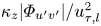 $\kappa _z|\varPhi _{u'v'}|/u_{\tau,l}^{2}$ with grey levels in $[0,0.4]$ with a $0.02$ increment. Colour lines have the same meaning as in figure 13.

Finally, we consider the magnitude of the co-spectra of the Reynolds shear stress shown in panels (d,h). As we said, these co-spectra are an indicator of the large spanwise rollers that in these cases are triggered by the KH instability at the canopy tip. Here, it is worth noticing how the large structures penetrate deeply in the canopy layer when the stems are inclined backwardly (panel h), moving the centre of the vortices well within the canopy layer. This explains the drag-increasing effect of the negative inclination: the large vortices are pushed in the canopy layer that dissipates, through the drag, the high momentum carried by those structures, thus requiring more energy to move the flow. The considerations made above are valid in the case of inclined canopies in the limit of a transitional to dense regime. Further inclining the stems eventually brings to a flow over a solid wall characterized by filamentous patterns of roughness, with size of the order of the diameter of the stems,  $d$, with the direction of the inclination disappearing from the parameters. Therefore, the structures of the two oppositely very-inclined cases considered in our study have a similar morphology between them and, approaching the sparsity of the canopy layer (Nepf Reference Nepf2012; Brunet Reference Brunet2020), behave very differently compared to the cases with $|\theta |=45^{\circ }$. Figures 17 and 18 show the velocity structures of the two cases considered (top row $\theta =78.5^{\circ }$ and bottom row $\theta =-78.5^{\circ }$) as a function of the streamwise and spanwise wavelengths, respectively. The sets of figures show, as expected, very similar coherency between the positively and negatively inclined canopies, with slight differences within the canopy layer in the energy content of the streamwise component of the velocity fluctuations (and consequently of the Reynolds shear stress) due to the different penetration of the outer layer imposed by the direction of the inclination. Finally, concerning the morphology of the coherent structures, figures 17 and 18 reveal that the outer layer, as we expect from a canopy flow in a quasi-sparse regime, is able to penetrate fully within the canopy layer, with the inner peaks that are simply an extension of the structures populating the outer boundary layer, only shortened by the presence of the stems.
Cases  $\theta =\pm 78.5^{\circ }$. Magnitude of the premultiplied spectra of the velocity components and co-spectra of the Reynolds shear stress as a function of the streamwise wavelength $\lambda _x/H$ and the wall-normal coordinates $y/H$: (a–d) $\theta =78.5^{\circ }$; (e–h) $\theta =-78.5^{\circ }$. The plots show: (a,e) $\kappa _x\varPhi _{u'u'}/u_{\tau,l}^{2}$ with grey levels in $[0,0.8]$ with a $0.1$ increment; (b, f) $\kappa _x\varPhi _{v'v'}/u_{\tau,l}^{2}$ with grey levels in $[0,0.3]$ with a $0.03$ increment; (c,g) $\kappa _x\varPhi _{w'w'}/u_{\tau,l}^{2}$ with grey levels in $[0,0.5]$ with a $0.05$ increment; (d,h)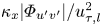 $\kappa _x|\varPhi _{u'v'}|/u_{\tau,l}^{2}$ with grey levels in $[0,0.4]$ with a $0.02$ increment. Colour lines have the same meaning as in figure 13.

Cases  $\theta =\pm 78.5^{\circ }$. Magnitude of the premultiplied spectra of the velocity components and co-spectra of the Reynolds shear stress as a function of the spanwise wavelength $\lambda _z/H$ and the wall-normal coordinates $y/H$: (a–d) $\theta =78.5^{\circ }$; (e–h) $\theta =-78.5^{\circ }$. The plots show: (a,e) $\kappa _z\varPhi _{u'u'}/u_{\tau,l}^{2}$ with grey levels in $[0,0.8]$ with a $0.1$ increment; (b, f) $\kappa _z\varPhi _{v'v'}/u_{\tau,l}^{2}$ with grey levels in $[0,0.3]$ with a $0.03$ increment; (c,g) $\kappa _z\varPhi _{w'w'}/u_{\tau,l}^{2}$ with grey levels in $[0,0.5]$ with a $0.05$ increment; (d,h)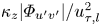 $\kappa _z|\varPhi _{u'v'}|/u_{\tau,l}^{2}$ with grey levels in $[0,0.4]$ with a $0.02$ increment. Colour lines have the same meaning as in figure 13.

At last, a further proof of the discrepancy of the properties of the flow attributed to the sign of the angle of inclination of the filaments can be sought in the joint probability density functions (j.p.d.f.s) of the fluctuations of the streamwise velocity  $u'$ and the wall-normal velocity $v'$. Figure 19 shows the contour lines (spacing 0.025, starting from the level 0.025 on the most external contour line) of the j.p.d.f. at three locations parallel to the wall for the cases $\theta =\pm 45^{\circ }$; such an angle $|\theta |$ is chosen as a case that well represents the discrepancy between the positive and negative inclination of the stems. The figure is organized in a $2\times 3$ matrix of panels, where the columns of the matrix, from left to right, shows the j.p.d.f. of $u'$–
$u'$– $v'$ at the location $y=0.10H< l_\perp$ (i.e. within the canopy layer), $y=l_\perp$ (the canopy edge), and $y=0.25H>l_\perp$ (i.e. above the canopy region) for the cases $\theta =45^{\circ }$ (top row) and $\theta =-45^{\circ }$ (bottom row). In the region above the canopy, the j.p.d.f. in figures 19(c, f) shows a similar distribution of $u'$–
$u'$– $v'$ for the two canopies analysed, with prevalence of events almost equally distributed within the second and fourth quadrants (ejections and sweeps, respectively), as has been observed in canopy flows (Bailey & Stoll Reference Bailey and Stoll2016). Moving towards the canopy region, the effect of the sign of the angle of inclination starts to appear. At first, we analyse the j.p.d.f. at the edge of the canopy, shown in figures 19(b,e). We can notice at once that both the distributions show two peaks: the smallest and very frequent one (higher number of levels) found on the left side of the figures with $u'<0$ and $v'\approx 0$ represents the recirculation forming behind each stem; the broadest one, instead, located within the second quadrant with $u'<0$ and $v'>0$, reports that ejections are the events that are more probable, especially for $\theta =-45^{\circ }$. The shape of the distributions for the two scenarios, however, is very similar, with only higher probability of $u'$–
$u'$– $v'$ (more contour levels) for the case inclined forwardly. Within the canopy layer, figures 19(a,d), instead, the scenario is very different: while the canopy inclined with the grain (figures 19(a–c) has a j.p.d.f. that keeps the shape of the upper layers, with a prevalence of events within the second quadrant, the canopy inclined against the grain (figures 19(d–f) has a j.p.d.f. that shows the appearance of events within the third quadrant, evidencing the eased capability of the flow to penetrate within the canopy. Finally, it is worth noticing the inclination of the peak related to the wakes of the filaments: while in the case with $\theta =45^{\circ }$ the wakes tend to have a positive $v'$, the opposite is true for the case with $\theta =-45^{\circ }$.
Cases  $\theta =\pm 45^{\circ }$. Contours of the joint probability function of the fluctuations of the streamwise velocity component $u'^{+}$ and the wall-normal velocity component $v'^{+}$, normalized with the local friction velocity $u_{\tau,l}$, on planes parallel to the wall: (a–c) $\theta =45^{\circ }$; (d–f) $\theta =-45^{\circ }$. The columns indicate the planes parallel to the wall: (a,d) $y=0.10H< l_\perp$; (b,e) $y=l_\perp$; (c, f) $y=0.25H>l_\perp$. The levels of the contour lines start from $0.025$ (most external line), and increase with increment $0.025$. The red dashed lines show the axes $u'=0$ and $v'=0$.

4. Conclusion
We have carried out a set of high-fidelity numerical simulations of a turbulent channel flow over inclined rigid canopies with the aim of (i) exploring the effectiveness of the solidity  $\lambda$ as selective parameter for determining the behaviour of canopy flows, and (ii) offering a complete description of the interaction between the coherent structures populating the inner and outer layers of the canopy flow.
At first, we have compared canopies inclined with opposite angles  $\theta$, finding that the stems inclined with the grain (i.e. $\theta > 0$) shield the canopy layer from the outer coherent motions, thus increasing the separation of the inner and outer layers while, on the contrary, filaments inclined against the grain (i.e. $\theta < 0$) promote the penetration of the high-momentum large coherent motions of the outer flow within the canopy layer. Since these large turbulent structures carry high momentum that is dissipated by the stems, canopies against the grain introduce a higher drag. Finally, very inclined canopies behave asymptotically as roughness, therefore losing their dependence from the angle of inclination. These considerations conclude that the solidity may be a misleading parameter for predicting the behaviour of canopy flows, and therefore a need for a more complex model rises. Here, based on the scaling of the pressure gradient, we proposed the outer quantities for the classification of the regimes.
In the second part of the paper, we have improved the description of mixing between the outer boundary layer and the inner flow. In particular, we started treating the two layers as separated: the structures of the inner layer can be compared to the high-speed and low-speed wakes generated passing through bidimensional cylinders, the former coming from the blockage effect, and the latter from the wakes of a bluff body; the outer layer, instead, is populated by large coherent motions triggered by the KH instability at the canopy tip. Following the work by Monti et al. (Reference Monti, Omidyeganeh, Eckhardt and Pinelli2020), we suggest that the two layers communicate through a set of high-momentum large wall-normal jets (Banyassady & Piomelli Reference Banyassady and Piomelli2015) that detach from the outer coherent structures and penetrate within the canopy as a result of its high wall-normal permeability. At the wall, these jets trigger the formation of the very-large coherent motions of  $u'$ and $w'$ observed in proximity to the canopy bed. By reflection, outside the region of the jets, the flow is pushed gently away from the wall, creating regions of $u'v'$ vortices similar to KH; this mechanism fixes the location of the inner inflection point. Inclining the stems of the canopy, the mechanism of interaction is magnified or reduced depending on the direction of the inclination. In particular, when the canopy is inclined against the grain ( $\theta <0$), the outer large structures are able to penetrate deeply within the canopy, with stronger wall-normal jets that energize the flow within the canopy layer; on the contrary, when the canopy is inclined with the grain, the inclined stems shelter the inner region, impeding the structures populating the boundary layer above the canopy to interact with the structures living close to the wall. However, this effect of the inclination tends to vanish when the height of the canopy layer becomes very small (very high $|\theta |$), since the latter tends to become roughness (sparse regime), and the outer and inner structures become very well mixed.
The natural extension of the present research consists in considering the flexibility of the stems of the canopy as an additional parameter. When the flexibility of the filaments is introduced, the complexity of flow increases considerably due to the coupling between the fluid and the structural elements, with the latter moving compliantly with the flow, thus having a variable and non-uniform inclination induced by the presence of the strong coherent structures of the outer energetic layer.
Funding
M.E.R. and A.M. gratefully acknowledge the support of the Okinawa Institute of Science and Technology Graduate University (OIST) with subsidy funding from the Cabinet Office, Government of Japan. M.E.R. and A.M. acknowledge the computational time provided by HPCI on the Oakbridge-CX and Oakforest-PACS clusters, under the grant hp210025, and the computer time provided by the Scientific Computing section of Research Support Division at OIST.
Declaration of interests
The authors report no conflict of interest.


 Open access

