





1. Introduction
Improving our fundamental understanding of high Reynolds number ( ${\textit{Re}}$
) turbulent boundary layers requires advancements in both experimental methods as well as simulation techniques. This would, for instance, enable us to answer questions such as the extent of applicability of Taylor’s hypothesis by knowing the scale-dependent distribution of convection velocities, to unravel the influence of large-scale structures on near-wall turbulence or to find out the differences between canonical cases of wall turbulence, viz., pipes (Massaro et al. Reference Massaro, Yao, Rezaeiravesh, Hussain and Schlatter2024b
), channels (Monty et al. Reference Monty, Stewart, Williams and Chong2007, Reference Monty, Hutchins, H.C.H., Marusic and Chong2009) and turbulent boundary layers (Hutchins & Marusic Reference Hutchins and Marusic2007; Smits, McKeon & Marusic Reference Simens, Jiménez, Hoyas and Mizuno2011).
${\textit{Re}}$
) turbulent boundary layers requires advancements in both experimental methods as well as simulation techniques. This would, for instance, enable us to answer questions such as the extent of applicability of Taylor’s hypothesis by knowing the scale-dependent distribution of convection velocities, to unravel the influence of large-scale structures on near-wall turbulence or to find out the differences between canonical cases of wall turbulence, viz., pipes (Massaro et al. Reference Massaro, Yao, Rezaeiravesh, Hussain and Schlatter2024b
), channels (Monty et al. Reference Monty, Stewart, Williams and Chong2007, Reference Monty, Hutchins, H.C.H., Marusic and Chong2009) and turbulent boundary layers (Hutchins & Marusic Reference Hutchins and Marusic2007; Smits, McKeon & Marusic Reference Simens, Jiménez, Hoyas and Mizuno2011).
The focus of this current work is on simulation methods for spatially developing turbulent boundary layers, where the turbulence inflow condition is often a limiting factor. We note that an alternative approach is to consider a so-called temporally developing boundary layer (Spalart Reference Smits, McKeon and Marusic1988; Biau Reference Biau2023; Wynn et al. Reference Wu2025), which is streamwise periodic. However, spatially developing layers are naturally occurring phenomena crucial to many industrial applications. This justifies the need to further develop a simulation methodology for their study.
A good turbulent inflow method is expected to develop the flow to the required turbulent state in as short a streamwise distance as possible (Tabor & Baba-Ahmadi Reference Subrahmanyam, Cantwell and Alonso2010). This becomes difficult at higher ${\textit{Re}}$
, because the large structures in the outer region take longer to develop (Sillero, Jiménez & Moser Reference Schlatter and Örlü2013). Wu (Reference Wei, Li and Wang2017) and Dhamankar, Blaisdell & Lyrintzis (Reference Dhamankar, Blaisdell and Lyrintzis2018) provide a concise overview of several methods that can be used to provide an inflow condition. In principle, we can distinguish two basic types: (i) methods that re-use real turbulent fields after some transformation and (ii) methods that create artificial turbulence, and mixtures of the two. Generally, artificially generating turbulence incurs little computational overhead, but leads to a larger development length. On the other hand, precursor-based methods provide high-quality inflow, but require an additional simulation, the cost of which grows with
${\textit{Re}}$
, because the large structures in the outer region take longer to develop (Sillero, Jiménez & Moser Reference Schlatter and Örlü2013). Wu (Reference Wei, Li and Wang2017) and Dhamankar, Blaisdell & Lyrintzis (Reference Dhamankar, Blaisdell and Lyrintzis2018) provide a concise overview of several methods that can be used to provide an inflow condition. In principle, we can distinguish two basic types: (i) methods that re-use real turbulent fields after some transformation and (ii) methods that create artificial turbulence, and mixtures of the two. Generally, artificially generating turbulence incurs little computational overhead, but leads to a larger development length. On the other hand, precursor-based methods provide high-quality inflow, but require an additional simulation, the cost of which grows with ${\textit{Re}}$
. Having means to reduce this cost would therefore be extremely beneficial. In this work, we propose a novel way to do that.
${\textit{Re}}$
. Having means to reduce this cost would therefore be extremely beneficial. In this work, we propose a novel way to do that.
Central to our approach is the idea to utilise the known structure of the coherent eddies (Robinson Reference Rezaeiravesh, Jansson, Peplinski, Vincent and Schlatter1991) within a turbulent boundary layer to derive the inflow generation procedure. The underlying theory stems from the works of Perry & Chong (Reference Perez, Toosi, Olsen, Markidis and Schlatter1982), Perry & Marušić (Reference Perry and Chong1995) and Marušić & Perry (Reference Marušić and Perry1995), who demonstrated, using the attached eddy hypothesis of Townsend (Reference Touber and Sandham1956, Reference Townsend1976), that the first- and second-order statistics of a turbulent boundary layer can be reproduced using a superposition of these coherent structures. A short overview of previous works that tried to leverage this follows.
Subbareddy et al. (Reference Stanly, Du, Xavier, Perez, Mukha, Markidis, Rezaeiravesh and Schlatter2006) proposed an inflow condition where they assumed the flow was populated by hairpin vortices with a given population density. The Biot–Savart law was used to compute the velocity field these vortices induced around them and image vortices at the wall were used to enforce the no-penetration condition. However, they mentioned that it ‘would be impractical to resolve’ the inner-scale structures ‘at moderate to high Reynolds number’ flows using this idea ‘on small/medium sized grids’ and that the method was better suited for large-eddy simulation (LES) or hybrid Reynolds-Averaged Navier–Stokes-LES which did not resolve the wall. Sandham, Yao & Lawal (Reference Sandberg and Sandham2003) proposed a simple coherent structure-based model which split the boundary layer into two regions: an inner region populated with lifted streaks and an outer region populated with three-dimensional eddies. Their deterministic model introduced disturbances corresponding to the inner and outer regions along with their associated phase information. Touber & Sandham (Reference Tabor and Baba-Ahmadi2009) later evaluated this method and found that it generated a mean velocity profile with an unrealistic outer region, and resulted in a spurious secondary peak in turbulence intensity and Reynolds shear-stress profiles in the outer region. These could be corrected by running several precursors and tuning certain parameters as in Sandberg & Sandham (Reference Robinson2008) and Sandham & Sandberg (Reference Sandham, Yao and Lawal2009). In another work, Pamiès et al. (Reference Örlü and Schlatter2009) proposed a modification to the synthetic eddy method by Jarrin et al. (Reference Jarrin, Benhamadouche, Laurence and Prosser2006) for LES of spatially developing boundary layers. They split the random structures into those belonging to different modes and included their proper length, time, velocity and vorticity contents, to better represent the vortex structures inside a turbulent boundary layer in the wall-normal direction. With this they were able to better specify the information of the modes for the buffer and logarithmic layers which helped reduce their development length.
Pre-multiplied spectra of streamwise velocity $u$
at increasing
$u$
at increasing ${\textit{Re}}$
(
${\textit{Re}}$
( $ {\textit{Re}}_\theta =2240, 4430, 8000$
; contour lines of increasing darkness show increasing
$ {\textit{Re}}_\theta =2240, 4430, 8000$
; contour lines of increasing darkness show increasing ${\textit{Re}}$
), i.e.
${\textit{Re}}$
), i.e. $E_{\textit{uu}}(k_z)\boldsymbol{\cdot }k_z /u_\tau ^2$
. Here,
$E_{\textit{uu}}(k_z)\boldsymbol{\cdot }k_z /u_\tau ^2$
. Here, $y$
is the wall-normal coordinate. Notice that the inner region (left of the vertical dashed line) remains the same size, whereas the outer region (right of the vertical dashed line) grows with increasing
$y$
is the wall-normal coordinate. Notice that the inner region (left of the vertical dashed line) remains the same size, whereas the outer region (right of the vertical dashed line) grows with increasing ${\textit{Re}}$
. For each level of darkness, contour lines are plotted for levels
${\textit{Re}}$
. For each level of darkness, contour lines are plotted for levels $[0.5, 1.5, 2.5, 4.0]$
. Data from Eitel-Amor, Örlü & Schlatter (Reference Eitel-Amor, Örlü and Schlatter2014).
$[0.5, 1.5, 2.5, 4.0]$
. Data from Eitel-Amor, Örlü & Schlatter (Reference Eitel-Amor, Örlü and Schlatter2014).

While the above studies focused on artificial turbulence, we seek to leverage the same theory but in the context of precursor-based inflow generation. In particular, the proposed method relies on the observed energy scaling of coherent structures in spectral space. The inner-scaled spectra of streamwise velocity pre-multiplied with spanwise wavenumbers (figure 1) show that with an increase in ${\textit{Re}}$
the outer region grows and occupies more spanwise wavenumbers as opposed to the inner region that remains nearly unchanged. It follows that given cross-stream velocity slices at a given
${\textit{Re}}$
the outer region grows and occupies more spanwise wavenumbers as opposed to the inner region that remains nearly unchanged. It follows that given cross-stream velocity slices at a given ${\textit{Re}}$
, a higher-
${\textit{Re}}$
, a higher- ${\textit{Re}}$
inflow could be produced by a rescaling of the outer-layer structures in the original data.
${\textit{Re}}$
inflow could be produced by a rescaling of the outer-layer structures in the original data.
Using the proposed method, time-dependent cross-stream velocity slices of a turbulent boundary layer at a given ${\textit{Re}}$
are first split into inner and outer regions in spectral space, followed by scaling (in space, time and energy) of the spanwise wavenumbers corresponding to the outer region appropriately to then reconstruct velocity fields at any higher
${\textit{Re}}$
are first split into inner and outer regions in spectral space, followed by scaling (in space, time and energy) of the spanwise wavenumbers corresponding to the outer region appropriately to then reconstruct velocity fields at any higher ${\textit{Re}}$
of interest. As schematically shown in figure 2, such a procedure enables a leap from low
${\textit{Re}}$
of interest. As schematically shown in figure 2, such a procedure enables a leap from low ${\textit{Re}}$
precursor data to much higher
${\textit{Re}}$
precursor data to much higher ${\textit{Re}}$
. This avoids the need for prohibitively expensive precursor domains, which must be larger the higher the target
${\textit{Re}}$
. This avoids the need for prohibitively expensive precursor domains, which must be larger the higher the target ${\textit{Re}}$
one aims to simulate.
${\textit{Re}}$
one aims to simulate.
In the remainder of this paper, we first describe the scaling method in detail in § 2, followed by demonstrating its application as inflow condition in § 3. Final conclusions and outlook are given in § 4.
Schematic of the proposed method highlighting its potential to reduce computational cost by up-scaling low- ${\textit{Re}}$
precursor data to high
${\textit{Re}}$
precursor data to high ${\textit{Re}}$
. (a) In classic precursor or existing methods, the precursor domain must grow with the target
${\textit{Re}}$
. (a) In classic precursor or existing methods, the precursor domain must grow with the target ${\textit{Re}}$
. (b) The proposed scaling method enables a small, fixed-size precursor domain regardless of target
${\textit{Re}}$
. (b) The proposed scaling method enables a small, fixed-size precursor domain regardless of target ${\textit{Re}}$
. Black dashed boxes show precursor domains; grey dashed boxes show main turbulent boundary layer (TBL) simulation domains. Single-lined arrows indicate flow direction, double-lined arrows indicate Dirichlet inflow application.
${\textit{Re}}$
. Black dashed boxes show precursor domains; grey dashed boxes show main turbulent boundary layer (TBL) simulation domains. Single-lined arrows indicate flow direction, double-lined arrows indicate Dirichlet inflow application.

2. Methodology
Necessary notation is now introduced before proceeding with a detailed description of the proposed inflow generation method. The superscript tg will be used to denote quantities at the target Reynolds number, ${\textit{Re}}^{\textit{tg}}$
, at which the inflow is to be generated. Similarly, the superscript bs will denote quantities already available at some base Reynolds number,
${\textit{Re}}^{\textit{tg}}$
, at which the inflow is to be generated. Similarly, the superscript bs will denote quantities already available at some base Reynolds number, ${\textit{Re}}^{\textit{bs}} \lt {\textit{Re}}^{\textit{tg}}$
. Further,
${\textit{Re}}^{\textit{bs}} \lt {\textit{Re}}^{\textit{tg}}$
. Further, $u_i$
will refer to the Cartesian projections of the velocity field, where
$u_i$
will refer to the Cartesian projections of the velocity field, where $i \in \{1, 2, 3\}$
denotes the coordinate index. The values of
$i \in \{1, 2, 3\}$
denotes the coordinate index. The values of $i$
correspond to the streamwise, wall-normal and spanwise directions. The triples (
$i$
correspond to the streamwise, wall-normal and spanwise directions. The triples ( $x$
,
$x$
, $y$
,
$y$
, $z$
) and (
$z$
) and ( $u$
,
$u$
, $v$
,
$v$
, $w$
) will also be used for the coordinates and velocity components, respectively. Similarly,
$w$
) will also be used for the coordinates and velocity components, respectively. Similarly, $U_i$
will denote the mean value of
$U_i$
will denote the mean value of $u_i$
, and a prime will be used for fluctuations, i.e.
$u_i$
, and a prime will be used for fluctuations, i.e. $u_i = U_i + u'_i$
. The root-mean-square values of the fluctuations will be referred to as
$u_i = U_i + u'_i$
. The root-mean-square values of the fluctuations will be referred to as $u_{\textit{rms}}$
,
$u_{\textit{rms}}$
, $v_{\textit{rms}}$
and
$v_{\textit{rms}}$
and $w_{\textit{rms}}$
. The
$w_{\textit{rms}}$
. The $+$
superscript will be used to denote scaling with inner-layer quantities, that is, the friction velocity
$+$
superscript will be used to denote scaling with inner-layer quantities, that is, the friction velocity $u_\tau$
and inner length scale
$u_\tau$
and inner length scale $l^*$
. The velocity of the free stream will be referred to as
$l^*$
. The velocity of the free stream will be referred to as $U_{\infty }$
. Finally, the boundary layer thickness will be quantified in terms of momentum-loss thickness,
$U_{\infty }$
. Finally, the boundary layer thickness will be quantified in terms of momentum-loss thickness, $\theta$
, and the wall-normal location where
$\theta$
, and the wall-normal location where $U_1 = 0.99U_{\infty }$
, i.e.
$U_1 = 0.99U_{\infty }$
, i.e. $\delta _{99}$
. The corresponding Reynolds numbers are
$\delta _{99}$
. The corresponding Reynolds numbers are ${\textit{Re}}_\theta$
and
${\textit{Re}}_\theta$
and ${\textit{Re}}_{\delta _{99}}$
. Additional notation will be introduced as necessary.
${\textit{Re}}_{\delta _{99}}$
. Additional notation will be introduced as necessary.
The Matlab implementation of the proposed method is available at https://github.com/ronithstanly/scaling_inflow and the time series data of velocity slices at ${\textit{Re}}^{\textit{bs}}$
, from Eitel-Amor et al. (Reference Eitel-Amor, Örlü and Schlatter2014), used in this work can be made available upon request.
${\textit{Re}}^{\textit{bs}}$
, from Eitel-Amor et al. (Reference Eitel-Amor, Örlü and Schlatter2014), used in this work can be made available upon request.
To obtain velocity fields at $ {\textit{Re}}^{\textit{tg}}$
, the proposed method requires the following two inputs:
$ {\textit{Re}}^{\textit{tg}}$
, the proposed method requires the following two inputs:
-
(i) Time-dependent cross-stream velocity slices at a lower $ {\textit{Re}}^{\textit{bs}}$
.
$ {\textit{Re}}^{\textit{bs}}$
. -
(ii) The target
${}\, {\textit{Re}}^{\textit{tg}}$
.


And, if the flow is not a generic zero-pressure-gradient TBL, appropriate scaling behaviour of the velocity spectral density and velocity profiles.
Using the value of $ {\textit{Re}}^{\textit{tg}}$
, the following derived inputs are calculated: mean velocity profiles
$ {\textit{Re}}^{\textit{tg}}$
, the following derived inputs are calculated: mean velocity profiles $U^{\textit{tg}}_{i}(y)$
and the scaling factors for the outer-layer structures in space and time (
$U^{\textit{tg}}_{i}(y)$
and the scaling factors for the outer-layer structures in space and time ( $S_{\delta _{99}}$
), and energy (
$S_{\delta _{99}}$
), and energy ( $S_{E}$
).
$S_{E}$
).
The velocity fields at $ {\textit{Re}}^{\textit{bs}}$
can be obtained by running a low-cost precursor, or simply taken from an existing database. The slices should be wide enough in
$ {\textit{Re}}^{\textit{bs}}$
can be obtained by running a low-cost precursor, or simply taken from an existing database. The slices should be wide enough in $z$
to incorporate the wider structures that would appear after applying the rescaling procedure. Otherwise, the enforced spanwise periodicity will introduce artificial correlations into the flow. Potential alternatives to avoid a very wide domain in the precursor are discussed in § 4.
$z$
to incorporate the wider structures that would appear after applying the rescaling procedure. Otherwise, the enforced spanwise periodicity will introduce artificial correlations into the flow. Potential alternatives to avoid a very wide domain in the precursor are discussed in § 4.
An additional requirement is that, at $ {\textit{Re}}^{\textit{bs}}$
, the flow should have some large-scale structures present beyond an inner-scaled spanwise wavelength of
$ {\textit{Re}}^{\textit{bs}}$
, the flow should have some large-scale structures present beyond an inner-scaled spanwise wavelength of $\lambda _z^+\gt 500$
, as seen in pre-multiplied spectra of streamwise velocity (figure 1). In other words,
$\lambda _z^+\gt 500$
, as seen in pre-multiplied spectra of streamwise velocity (figure 1). In other words, $ {\textit{Re}}^{\textit{bs}}$
should be high enough for outer scaling to be valid.
$ {\textit{Re}}^{\textit{bs}}$
should be high enough for outer scaling to be valid.
In this work, we use the database of Eitel-Amor et al. (Reference Eitel-Amor, Örlü and Schlatter2014), where a finely resolved LES was performed up to $ {\textit{Re}}_\theta =8300$
. Time series of cross-stream velocity slices sampled on a coarser
$ {\textit{Re}}_\theta =8300$
. Time series of cross-stream velocity slices sampled on a coarser $y$
-grid (of 47 points) are available at
$y$
-grid (of 47 points) are available at ${\textit{Re}}_\theta =2240, 3740, 4430, 5740$
and
${\textit{Re}}_\theta =2240, 3740, 4430, 5740$
and $8000$
.
$8000$
.
As will be shown below, $ {\textit{Re}}^{\textit{bs}}_\theta =2240$
is sufficiently high for the proposed method to work seamlessly (i.e. being able to scale velocity slices from
$ {\textit{Re}}^{\textit{bs}}_\theta =2240$
is sufficiently high for the proposed method to work seamlessly (i.e. being able to scale velocity slices from $ {\textit{Re}}^{\textit{bs}}_\theta$
to
$ {\textit{Re}}^{\textit{bs}}_\theta$
to $ {\textit{Re}}^{\textit{tg}}_\theta$
without knowing the shape of the spectra at
$ {\textit{Re}}^{\textit{tg}}_\theta$
without knowing the shape of the spectra at $ {\textit{Re}}^{\textit{tg}}_\theta$
). On the other hand, the extreme case of using a very low
$ {\textit{Re}}^{\textit{tg}}_\theta$
). On the other hand, the extreme case of using a very low $ {\textit{Re}}^{\textit{bs}}_\theta =790$
requires hand tuning of the scaling parameters for space and energy by examining an existing database of pre-multiplied spectra of
$ {\textit{Re}}^{\textit{bs}}_\theta =790$
requires hand tuning of the scaling parameters for space and energy by examining an existing database of pre-multiplied spectra of $u$
at
$u$
at $ {\textit{Re}}^{\textit{tg}}$
. This is because the outer scaling does not hold true at such a low Re where viscous effects and interactions between the inner and outer regions are strong.
$ {\textit{Re}}^{\textit{tg}}$
. This is because the outer scaling does not hold true at such a low Re where viscous effects and interactions between the inner and outer regions are strong.
The mean streamwise velocity profile at any $ {\textit{Re}}^{\textit{tg}}$
can be obtained by using, for instance, the log law (Von Kármán Reference Trefethen1930), Coles’ law (Coles Reference Coles1956), the composite profile (Monkewitz, Chauhan & Nagib Reference Monkewitz, Chauhan and Nagib2007) or any other suitable universal profile (Subrahmanyam, Cantwell & Alonso Reference Subbareddy, Peterson, Candler and Marusic2022). For the mean wall-normal velocity profile, methods like the ones proposed by Wei, Li & Wang (Reference Von Kármán2023) can be used. Alternatively, the continuity equation along with self-similarity can be employed to derive approximations. For the numerical experiments performed in this work, the database contained the information at
$ {\textit{Re}}^{\textit{tg}}$
can be obtained by using, for instance, the log law (Von Kármán Reference Trefethen1930), Coles’ law (Coles Reference Coles1956), the composite profile (Monkewitz, Chauhan & Nagib Reference Monkewitz, Chauhan and Nagib2007) or any other suitable universal profile (Subrahmanyam, Cantwell & Alonso Reference Subbareddy, Peterson, Candler and Marusic2022). For the mean wall-normal velocity profile, methods like the ones proposed by Wei, Li & Wang (Reference Von Kármán2023) can be used. Alternatively, the continuity equation along with self-similarity can be employed to derive approximations. For the numerical experiments performed in this work, the database contained the information at $ {\textit{Re}}^{\textit{tg}}$
, so the mean velocity profiles are taken from there.
$ {\textit{Re}}^{\textit{tg}}$
, so the mean velocity profiles are taken from there.
2.1. Extracting inner and outer structures
A discrete Fourier transform (DFT) is used to extract structures corresponding to the inner and outer regions from the velocity slices at $ {\textit{Re}}^{\textit{bs}}$
. The transform is applied along
$ {\textit{Re}}^{\textit{bs}}$
. The transform is applied along $z$
in lieu of periodicity of the flow in that direction. The transform is defined as
$z$
in lieu of periodicity of the flow in that direction. The transform is defined as
 \begin{equation} \hat {u}_i^{(k_z)}(y,t) = \frac {1}{\sqrt {n_z}} \sum _{j=0}^{n_z-1} u_i\big(y,z_j,t\big) e^{-2\pi i k_z j / n_z}. \end{equation}
The normalisation using $\sqrt {n_z}$
ensures that the Parseval relation holds (Trefethen Reference Townsend2000; Bounchaleun Reference Bounchaleun2019). Here, the wavenumber index
$\sqrt {n_z}$
ensures that the Parseval relation holds (Trefethen Reference Townsend2000; Bounchaleun Reference Bounchaleun2019). Here, the wavenumber index $k_z$
is related to the physical wavenumber
$k_z$
is related to the physical wavenumber $k_z^{\textit{phys}}$
as
$k_z^{\textit{phys}}$
as
 \begin{equation} k_z^{\textit{phys}} = \frac {2\pi k_z}{L_z}, \end{equation}
where $L_z$
is the size of the domain in
$L_z$
is the size of the domain in $z$
.
$z$
.
Because the velocity field is real valued, we exploit the Hermitian symmetry of the DFT and retain only one half of the wavenumbers
 \begin{equation} k_z \in \left [ 0, 1, 2, \ldots , \frac {n_z}{2} \right ]. \end{equation}
This modifies the normalisation factor in (2.1) to $\sqrt {n_z/2}$
.
$\sqrt {n_z/2}$
.
Following this, spanwise wavenumbers corresponding to the inner and outer regions of the TBL are extracted depending on their corresponding value of ${\lambda _z}^+$
which is calculated as
${\lambda _z}^+$
which is calculated as
 \begin{equation} {\lambda _z}^+ = \frac {2\pi }{k_{z}l^{*}}, \end{equation}
obtained as $l^*=\nu /u_{\tau }$
. Here,
$l^*=\nu /u_{\tau }$
. Here, $u_{\tau }$
is the friction velocity calculated using wall-shear stress
$u_{\tau }$
is the friction velocity calculated using wall-shear stress ${\tau }_w$
and density
${\tau }_w$
and density $\rho$
, as
$\rho$
, as $u_{\tau }=\sqrt {{\tau }_w/\rho }$
. Following this, a range of
$u_{\tau }=\sqrt {{\tau }_w/\rho }$
. Following this, a range of $k_z$
values corresponding approximately to
$k_z$
values corresponding approximately to $30 \leqslant {\lambda _{z}}^+\leqslant 500$
is extracted to obtain the inner region (i.e.
$30 \leqslant {\lambda _{z}}^+\leqslant 500$
is extracted to obtain the inner region (i.e. $k_z^{\textit{inner}}$
). For the outer region, the relevant range of
$k_z^{\textit{inner}}$
). For the outer region, the relevant range of $k_z$
(i.e.
$k_z$
(i.e. $k_z^{\textit{outer}}$
) depends on
$k_z^{\textit{outer}}$
) depends on $ {\textit{Re}}^{\textit{bs}}$
(see figure 1). For instance, for
$ {\textit{Re}}^{\textit{bs}}$
(see figure 1). For instance, for $ {\textit{Re}}_{\theta }=2240$
,
$ {\textit{Re}}_{\theta }=2240$
, $k_z^{\textit{outer}}$
is approximately
$k_z^{\textit{outer}}$
is approximately $500 \lt {\lambda _{z}}^+\leqslant 1700$
, and for
$500 \lt {\lambda _{z}}^+\leqslant 1700$
, and for $ {\textit{Re}}_{\theta }=4430$
it shifts to
$ {\textit{Re}}_{\theta }=4430$
it shifts to $750 \lt {\lambda _{z}}^+\leq 3000$
.
$750 \lt {\lambda _{z}}^+\leq 3000$
.
The $\hat {u_i}^{(k_z)}(y,t)$
for the selected wavenumbers are stacked into adjacent columns to construct the complex snapshot matrix. Singular value decomposition (SVD) is then performed in the wall-normal direction for each of those wavenumbers. This results in time coefficients,
$\hat {u_i}^{(k_z)}(y,t)$
for the selected wavenumbers are stacked into adjacent columns to construct the complex snapshot matrix. Singular value decomposition (SVD) is then performed in the wall-normal direction for each of those wavenumbers. This results in time coefficients, $a^{(k_{z},n)}(t)$
of the
$a^{(k_{z},n)}(t)$
of the $n$
th proper orthogonal decomposition (POD) mode, and complex POD modes,
$n$
th proper orthogonal decomposition (POD) mode, and complex POD modes, $\hat {\varphi _i}^{(k_z,n)}(y)$
. The above operations result in an expansion as follows:
$\hat {\varphi _i}^{(k_z,n)}(y)$
. The above operations result in an expansion as follows:
 \begin{equation} \hat {u_i}^{(k_z)}(y,t) \approx \sum \limits ^{n_{\textit{modes}}-1}_{n=0}a^{(k_z,n)}(t)\hat {\varphi _i}^{(k_z,n)}(y). \end{equation}
The time coefficients are used to scale the temporal evolution of those selected structures, as shown below. The SVD enables two extra possibilities: (i) to create a low-order model for the wall-normal dynamics, and (ii) to incorporate synthetically extended time coefficients generated by vector autoregression as described by Stanly et al. (Reference Stanly, Bagheri, Mukha and Schlatter2024). The latter provides a way to extend the time duration of the generated inflow beyond that of the precursor database. However, in principle, the SVD can be omitted and the rescaling performed directly on the Fourier coefficients.
2.2. Scaling procedure
Overall, scaling the velocity fields in ${\textit{Re}}$
involves shifting the spanwise wavenumbers of the selected structures, scaling the relevant modes in
${\textit{Re}}$
involves shifting the spanwise wavenumbers of the selected structures, scaling the relevant modes in $y$
and
$y$
and $t$
, as well as scaling their energy. In principle, the inner region is to be scaled in inner units and the outer region in outer units. However, it is known, for instance from Eitel-Amor et al. (Reference Eitel-Amor, Örlü and Schlatter2014), that the growth of the structures in the inner region of a TBL is almost negligible compared with the growth of the outer region as we go to higher
$t$
, as well as scaling their energy. In principle, the inner region is to be scaled in inner units and the outer region in outer units. However, it is known, for instance from Eitel-Amor et al. (Reference Eitel-Amor, Örlü and Schlatter2014), that the growth of the structures in the inner region of a TBL is almost negligible compared with the growth of the outer region as we go to higher ${\textit{Re}}$
. Moreover, the quickly evolving near-wall structures would compensate for these small differences quite rapidly, as opposed to the slow outer structures. For instance, when comparing
${\textit{Re}}$
. Moreover, the quickly evolving near-wall structures would compensate for these small differences quite rapidly, as opposed to the slow outer structures. For instance, when comparing $ {\textit{Re}}_\theta =2240$
with
$ {\textit{Re}}_\theta =2240$
with $ {\textit{Re}}_\theta =8000$
, the viscous length scale
$ {\textit{Re}}_\theta =8000$
, the viscous length scale $l^*$
increases by a factor of
$l^*$
increases by a factor of $1.16$
, whereas the boundary layer thickness
$1.16$
, whereas the boundary layer thickness $\delta _{99}$
increases by a factor of
$\delta _{99}$
increases by a factor of $3.96$
. Owing to this, in this work, the inner region from the base
$3.96$
. Owing to this, in this work, the inner region from the base $ {\textit{Re}}^{\textit{bs}}$
is kept as such, and only the outer region is scaled in outer units in our scaling procedure to reach the target
$ {\textit{Re}}^{\textit{bs}}$
is kept as such, and only the outer region is scaled in outer units in our scaling procedure to reach the target $ {\textit{Re}}^{\textit{tg}}$
.
$ {\textit{Re}}^{\textit{tg}}$
.
For the selected range of $k_z^{\textit{outer}}$
scaling is performed using the scaling factor,
$k_z^{\textit{outer}}$
scaling is performed using the scaling factor, $S_{\delta _{99}}$
, computed as
$S_{\delta _{99}}$
, computed as
 \begin{equation} S_{\delta _{99}} = \frac {{\delta _{99}}^{\textit{tg}}}{{\delta _{99}}^{\textit{bs}}}. \end{equation}
This scaling factor is 1.9 for the case where velocity slices at ${\textit{Re}}_\theta =4430$
are up-scaled to
${\textit{Re}}_\theta =4430$
are up-scaled to ${\textit{Re}}_\theta =8000$
, and 3.9 when
${\textit{Re}}_\theta =8000$
, and 3.9 when ${\textit{Re}}_\theta =2240$
are scaled up to
${\textit{Re}}_\theta =2240$
are scaled up to ${\textit{Re}}_\theta =8000$
.
${\textit{Re}}_\theta =8000$
.
2.2.1. Scaling in
$z$

Scaling in the spanwise direction $z$
is performed by means of shifting each of the
$z$
is performed by means of shifting each of the $n$
retained POD modes of the selected spanwise wavenumbers corresponding to the outer region,
$n$
retained POD modes of the selected spanwise wavenumbers corresponding to the outer region, $k_z^{\textit{outer}}$
, to the new position in spectral space. In this work, the first 40 POD modes are kept for all
$k_z^{\textit{outer}}$
, to the new position in spectral space. In this work, the first 40 POD modes are kept for all $k_z \in k_z^{\textit{outer}}$
. This preserves approximately
$k_z \in k_z^{\textit{outer}}$
. This preserves approximately $97\,\%$
of the turbulent kinetic energy (TKE) across the retained modes. Based on our previous work (Stanly et al. Reference Stanly, Bagheri, Mukha and Schlatter2024), this amount of TKE reduction had no noticeable negative effects on the inflow. Scaling in
$97\,\%$
of the turbulent kinetic energy (TKE) across the retained modes. Based on our previous work (Stanly et al. Reference Stanly, Bagheri, Mukha and Schlatter2024), this amount of TKE reduction had no noticeable negative effects on the inflow. Scaling in $z$
is performed as follows and is illustrated with an example in figure 3(a):
$z$
is performed as follows and is illustrated with an example in figure 3(a):
 \begin{equation} \hat {\varphi _i}^{\big({\textit{round}}\big(k_z/{S_{\delta _{99}}}\big),n\big)}(y) = \hat {\varphi _i}^{(k_z,n)}(y). \end{equation}
From here, we use $k_z^{\textit{outer}}$
to refer to the newly scaled/shifted range of outer
$k_z^{\textit{outer}}$
to refer to the newly scaled/shifted range of outer $k_z$
, i.e.
$k_z$
, i.e. $k_z^{\textit{outer}}\approx \text{\textit{round}}(k_z^{\textit{outer}}/S_{\delta _{99}})$
.
$k_z^{\textit{outer}}\approx \text{\textit{round}}(k_z^{\textit{outer}}/S_{\delta _{99}})$
.
2.2.2. Reconstruction of POD modes to physical space
Before applying further scaling operations, each POD mode can be independently reconstructed in physical space by applying an inverse Fourier transform to each wavenumber $k_z \in (k_z^{\textit{inner}} \cup k_z^{\textit{outer}})$
, i.e.
$k_z \in (k_z^{\textit{inner}} \cup k_z^{\textit{outer}})$
, i.e.
 \begin{equation} \varphi _i^{(k_z,n)}\big(y, z_j\big) = \frac {2}{\sqrt {n_z/2}} \hat {\varphi }_i^{(k_z,n)}(y) e^{2\pi i k_z j / n_z}, \end{equation}
where the factor $2$
, within and outside the square root, comes in as we retain only one half of the wavenumbers that exhibit Hermitian symmetry. The factor
$2$
, within and outside the square root, comes in as we retain only one half of the wavenumbers that exhibit Hermitian symmetry. The factor $2$
outside the square root can be removed if
$2$
outside the square root can be removed if $k_z \in (0,({n_z}/{2}))$
as they have no complex conjugate pairs.
$k_z \in (0,({n_z}/{2}))$
as they have no complex conjugate pairs.
2.2.3. Scaling in
$y$

Following this, each of the selected POD modes are to be scaled in the wall-normal direction $y$
, as the new structures would grow in
$y$
, as the new structures would grow in $y$
as well, when appearing at the higher
$y$
as well, when appearing at the higher ${\textit{Re}}$
. To achieve this, while keeping the POD modes the same, the
${\textit{Re}}$
. To achieve this, while keeping the POD modes the same, the $y$
axis is upscaled such that
$y$
axis is upscaled such that
 \begin{equation} y^{\textit{tg}} = y^{\textit{bs}} \boldsymbol{\cdot }S_{\delta _{99}}. \end{equation}
If one would now plot the POD modes using this new $y^{\textit{tg}}$
axis, the modes will look grown in the wall-normal coordinate. However, we need these grown modes on the same initial grid (i.e.
$y^{\textit{tg}}$
axis, the modes will look grown in the wall-normal coordinate. However, we need these grown modes on the same initial grid (i.e. $y^{\textit{bs}}$
). To get this, the next step is to chop off the
$y^{\textit{bs}}$
). To get this, the next step is to chop off the $y^{\textit{tg}}$
values beyond
$y^{\textit{tg}}$
values beyond $\text{max}(y^{\textit{bs}})$
such that both meshes go up to the same height. This would result in
$\text{max}(y^{\textit{bs}})$
such that both meshes go up to the same height. This would result in $\text{size}(y^{\textit{tg}})\lt \text{size}(y^{\textit{bs}})$
, in other words
$\text{size}(y^{\textit{tg}})\lt \text{size}(y^{\textit{bs}})$
, in other words $y^{\textit{tg}}$
ends up being coarser than
$y^{\textit{tg}}$
ends up being coarser than $y^{\textit{bs}}$
. To get back the scaled POD modes to the initial
$y^{\textit{bs}}$
. To get back the scaled POD modes to the initial $y^{\textit{bs}}$
, a two-dimensional spline interpolation is now performed
$y^{\textit{bs}}$
, a two-dimensional spline interpolation is now performed
 \begin{equation} {\varphi _i}^{\left(k_z,n\right)}\big(y^{\textit{tg}},z\big) \rightarrow {\varphi _i}^{\left(k_z,n\right)}\big(y^{\textit{bs}},z\big). \end{equation}
This scaling in $y$
is demonstrated in figure 3(b). Since the modes are mapped back to the initial grid (
$y$
is demonstrated in figure 3(b). Since the modes are mapped back to the initial grid ( $y^{\textit{bs}}$
) after scaling, the superscript is partially omitted in further discussions and just
$y^{\textit{bs}}$
) after scaling, the superscript is partially omitted in further discussions and just $y$
is used.
$y$
is used.
Effect of scaling in $k_z$
and
$k_z$
and $y$
, illustrated using the real part of the zeroth POD mode at
$y$
, illustrated using the real part of the zeroth POD mode at $k_z=10$
for the streamwise velocity component of re4k_sc, i.e.
$k_z=10$
for the streamwise velocity component of re4k_sc, i.e. $\text{Real}\{\varphi _1^{(k_z=10,n=0)}\}$
. In both (a) and (b), the lighter shade of blue shows the state before scaling, and the darker shade shows the state after scaling. For both, contour lines are plotted for levels
$\text{Real}\{\varphi _1^{(k_z=10,n=0)}\}$
. In both (a) and (b), the lighter shade of blue shows the state before scaling, and the darker shade shows the state after scaling. For both, contour lines are plotted for levels $[\pm 0.0015, \pm 0.0030, \pm 0.0045]$
. (a) Scaling in
$[\pm 0.0015, \pm 0.0030, \pm 0.0045]$
. (a) Scaling in $z$
, (b) scaling in
$z$
, (b) scaling in $y$
.
$y$
.

2.2.4. Scaling in
$t$

Next, the time coefficients have to be adjusted as the newly produced bigger structures in the outer region are expected to convect slower than the initial smaller counterparts. Thus, the time array is downscaled by $S_{\delta _{99}}$
. Subsequently, the new set of time coefficients are produced by interpolating the old ones on the new time axis. This can be shown as
$S_{\delta _{99}}$
. Subsequently, the new set of time coefficients are produced by interpolating the old ones on the new time axis. This can be shown as
 \begin{equation} t^{\textit{tg}} = t^{\textit{bs}} / S_{\delta _{99}}, \end{equation}
and for the coefficients
 \begin{equation} a^{(k_z,n)}\big(t^{\textit{bs}}\big) \rightarrow a^{(k_z,n)}\big(t^{\textit{tg}}\big). \end{equation}
2.2.5. Scaling the energy
For upscaling the energy of the outer structures, the square of the scaling factor ( ${S_{E}}^2$
) is computed between the mean streamwise turbulence intensity (
${S_{E}}^2$
) is computed between the mean streamwise turbulence intensity ( $u'u'$
) from the log and outer regions (say,
$u'u'$
) from the log and outer regions (say, $y^+\gt 100$
) of the base
$y^+\gt 100$
) of the base ${\textit{Re}}$
obtained from the database, and the mean streamwise turbulence intensity at the target
${\textit{Re}}$
obtained from the database, and the mean streamwise turbulence intensity at the target ${\textit{Re}}$
in the same region (i.e.
${\textit{Re}}$
in the same region (i.e. $y^+\gt 100$
). For the latter, the following expression proposed by Alfredsson, Segalini & Örlü (Reference Alfredsson, Segalini and Örlü2011) is used:
$y^+\gt 100$
). For the latter, the following expression proposed by Alfredsson, Segalini & Örlü (Reference Alfredsson, Segalini and Örlü2011) is used:
 \begin{equation} \frac {u^{\textit{tg}}_{\textit{rms}}\big(y^{\textit{bs}}\big)}{U^{\textit{tg}}_1\big(y^{\textit{bs}}\big)} = 0.031 + 0.260 \left ( 1-\frac {U^{\textit{tg}}_1\big(y^{\textit{bs}}\big)}{U_{\infty }} \right ). \end{equation}
Although this scaling factor for energy corresponds to the streamwise fluctuations alone, due to lack of other estimates to find scaling factors for fluctuations in the wall-normal and spanwise directions (and following some tests) the same factor is applied to upscale the energy of the wall-normal and spanwise fluctuations as well. This is done by multiplying this energy scaling factor to the corresponding outer modes of the three velocity components in the reconstruction phase. This scaling factor for energy is found to be $S_{E}\approx 1.3$
for the case where velocity slices at
$S_{E}\approx 1.3$
for the case where velocity slices at ${\textit{Re}}_\theta =4430$
are up-scaled to
${\textit{Re}}_\theta =4430$
are up-scaled to ${\textit{Re}}_\theta =8000$
, and
${\textit{Re}}_\theta =8000$
, and $S_{E}\approx 1.5$
when
$S_{E}\approx 1.5$
when ${\textit{Re}}_\theta =2240$
is scaled up to
${\textit{Re}}_\theta =2240$
is scaled up to ${\textit{Re}}_\theta =8000$
. This factor,
${\textit{Re}}_\theta =8000$
. This factor, $S_E$
, for energy is applied in the reconstruction phase that follows. Note that a POD mode needs to be scaled with the same factor in order to maintain mass conservation of the disturbances. This property is essential for high-fidelity inflow conditions, as e.g. discussed in Stanly et al. (Reference Spalart2026).
$S_E$
, for energy is applied in the reconstruction phase that follows. Note that a POD mode needs to be scaled with the same factor in order to maintain mass conservation of the disturbances. This property is essential for high-fidelity inflow conditions, as e.g. discussed in Stanly et al. (Reference Spalart2026).
2.3. Reconstruction
The generated mean velocity profiles, $U^{\textit{tg}}_{i}(y)$
, the selected inner modes and the scaled outer modes are used to reconstruct the velocity fields,
$U^{\textit{tg}}_{i}(y)$
, the selected inner modes and the scaled outer modes are used to reconstruct the velocity fields, $u^{\textit{tg}}_{i}(y,z,t^{\textit{tg}})$
, at the target Reynolds number. Note that the scaling of energy of the outer modes using the scaling factor
$u^{\textit{tg}}_{i}(y,z,t^{\textit{tg}})$
, at the target Reynolds number. Note that the scaling of energy of the outer modes using the scaling factor $S_{E}$
is performed at this stage. The reconstruction is mathematically formulated as follows:
$S_{E}$
is performed at this stage. The reconstruction is mathematically formulated as follows:
 \begin{align} u^{\textit{tg}}_{i}\big(y^{\textit{bs}},z,t^{\textit{tg}}\big) &= U^{\textit{tg}}_{i}\big(y^{\textit{bs}},z\big) \quad \text{(for } k_z = 0,\,n = 0\text{)} \nonumber\\ &\quad + \sum _{k_z\in k_z^{\textit{inner}}} \sum _{n=0}^{n_{\textit{modes}} - 1} a^{(k_z,n)}\big(t^{\textit{tg}}\big) \varphi _i^{(k_z,n)}\big(y^{\textit{bs}},z\big)\nonumber\\ &\quad + \sum _{k_z\in k_z^{\textit{outer}}} \sum _{n=0}^{n_{\textit{modes}} - 1} S_{E} \boldsymbol{\cdot }a^{(k_z,n)}\big(t^{\textit{tg}}\big) \varphi _i^{(k_z,n)}\big(y^{\textit{bs}},z\big). \end{align}
This entire process is outlined in Algorithm1, where $\mathcal{F}_z$
and
$\mathcal{F}_z$
and $\mathcal{F}_z^{-1}$
represent implementations of the fast Fourier transforms, such as the Matlab operations fft() and ifft(), i.e. the forward and inverse transform, respectively. The normalisations performed on them (i.e. on the output from these functions), in steps 1 and 11 using the factor
$\mathcal{F}_z^{-1}$
represent implementations of the fast Fourier transforms, such as the Matlab operations fft() and ifft(), i.e. the forward and inverse transform, respectively. The normalisations performed on them (i.e. on the output from these functions), in steps 1 and 11 using the factor $\sqrt {{n_z}/{2}}$
, yield (2.1) and (2.8) after accounting for the normalisation within these Matlab functions.
$\sqrt {{n_z}/{2}}$
, yield (2.1) and (2.8) after accounting for the normalisation within these Matlab functions.
3. Results
The proposed method is evaluated in two ways:
-
(i) Assessing the quality of the generated two-dimensional velocity slices that will be used as an inlet condition in § 3.1.
-
(ii) Applying those velocity planes as an inflow condition and analysing the evolution of a TBL starting at
${\textit{Re}}_\theta =8000$
in § 3.2.

To that end, time-dependent velocity slices at ${\textit{Re}}_\theta =2240$
and
${\textit{Re}}_\theta =2240$
and ${\textit{Re}}_\theta =4430$
from an available database (Eitel-Amor et al. Reference Eitel-Amor, Örlü and Schlatter2014) are scaled up to
${\textit{Re}}_\theta =4430$
from an available database (Eitel-Amor et al. Reference Eitel-Amor, Örlü and Schlatter2014) are scaled up to ${\textit{Re}}^{\textit{tg}}_\theta =8000$
using the proposed method and compared against the data at
${\textit{Re}}^{\textit{tg}}_\theta =8000$
using the proposed method and compared against the data at ${\textit{Re}}_\theta =8000$
available from the database.
${\textit{Re}}_\theta =8000$
available from the database.
These first two sets of scaled velocity planes will now be referred to as re2k_sc and re4k_sc, indicating the used $ {\textit{Re}}^{\textit{bs}}$
, and _sc showing that the data are scaled. The reference planes at
$ {\textit{Re}}^{\textit{bs}}$
, and _sc showing that the data are scaled. The reference planes at ${\textit{Re}}_\theta =8000$
will be referred to as re8k. Note that all three datasets are in principle at
${\textit{Re}}_\theta =8000$
will be referred to as re8k. Note that all three datasets are in principle at ${\textit{Re}}^{\textit{tg}}_\theta =8000$
. The TBL simulated using the re8k inflow data is essentially the classic precursor-based simulation.
${\textit{Re}}^{\textit{tg}}_\theta =8000$
. The TBL simulated using the re8k inflow data is essentially the classic precursor-based simulation.
By construction, the scaled velocity planes (re2k_sc and re4k_sc) have a gap in the pre-multiplied spectra (see figure 4
a), which needs to be filled up during adaptation. To examine if the scaled cases fill up this missing region in a reasonable way, we add an extra case for comparison. In particular, we modify the reference re8k data by removing spanwise wavenumbers approximately in the range $500\lt \lambda _z^+\lt 1400$
, thus introducing the
$500\lt \lambda _z^+\lt 1400$
, thus introducing the
Scaling of velocity fields from Rebs to Retg

Algorithm 1: Long description
An algorithm for scaling velocity fields from Rebs to Retg. Panel A: The algorithm starts with input variables u of b s (y b s, z, t b s) and Re t g, and derived input variables U of t g (y b s), S of 399, S of E, and n modes. The output is u of t g (y b s, z, t t g). Panel B: The algorithm performs a discrete Fourier transform in z, computes POD via singular value decomposition, classifies k z into inner and outer spectral ranges, scales in z, performs an inverse discrete Fourier transform, and reconstructs velocity fields at Re t g. Panel C: The algorithm involves upscaling the y-axis, removing y t g greater than maximum y b s, and interpolating POD modes and time coefficients.
same gap as in the scaled data. This additional set of planes is referred to as re8k_onlyIO, which stands for ‘only inner and outer’ regions. A summary of all four generated inflow datasets can be found in table 1.
Inflow datasets generated for the performance evaluation of the proposed method.

(a) One-dimensional pre-multiplied spectra of streamwise velocity $u$
, i.e.
$u$
, i.e. $E^+_{\textit{uu}}(k_z)\boldsymbol{\cdot }k_z$
, and (b) two-dimensional pre-multiplied power spectral density (PSD) of
$E^+_{\textit{uu}}(k_z)\boldsymbol{\cdot }k_z$
, and (b) two-dimensional pre-multiplied power spectral density (PSD) of $u$
in terms of
$u$
in terms of $\lambda _z^+$
and
$\lambda _z^+$
and $\lambda _t^+$
, i.e.
$\lambda _t^+$
, i.e. $E^+_{\textit{uu}}(k_t k_z)\boldsymbol{\cdot }k_t k_z$
, at
$E^+_{\textit{uu}}(k_t k_z)\boldsymbol{\cdot }k_t k_z$
, at $y\approx 0.2\delta _{99_0}$
(this height is marked using a dashed horizontal line in (a)). In both figures, the reference data re8k are shown in the background as filled contours using shades of grey with levels as shown in the colour bar. The re2k_sc, re4k_sc and re8k_onlyIO data are shown using green, blue and red contour lines, respectively, with the contour levels matching those used for the re8k data.
$y\approx 0.2\delta _{99_0}$
(this height is marked using a dashed horizontal line in (a)). In both figures, the reference data re8k are shown in the background as filled contours using shades of grey with levels as shown in the colour bar. The re2k_sc, re4k_sc and re8k_onlyIO data are shown using green, blue and red contour lines, respectively, with the contour levels matching those used for the re8k data.

3.1. Quality of the inflow velocity slices
The newly generated time-dependent, two-dimensional velocity slices of the cases re2k_sc and re4k_sc at the target ${\textit{Re}}^{\textit{tg}}_\theta =8000$
are assessed here in comparison with the reference re8k and re8k_onlyIO data, before applying them as an inflow condition in § 3.2.
${\textit{Re}}^{\textit{tg}}_\theta =8000$
are assessed here in comparison with the reference re8k and re8k_onlyIO data, before applying them as an inflow condition in § 3.2.
Reynolds stress profiles of the inlet velocity slices. Plot (a) shows the raw data whereas the data in (b) are obtained by applying a median filter to the raw data to facilitate visual inspection. The wiggles in the raw values are due to the coarse wall-normal resolution in the precursor data.

Figure 4(a) shows one-dimensional pre-multiplied spectra of streamwise velocity of the different cases. The gap in the spectra of the scaled cases (i.e. re2k_sc and re4k_sc), which arises due to the scaling procedure in $k_z$
(as described in § 2.2.1), as well as the intentional gap in re8k_onlyIO, are visible in the approximate range of
$k_z$
(as described in § 2.2.1), as well as the intentional gap in re8k_onlyIO, are visible in the approximate range of $500\lt \lambda _z^+\lt 1400$
. Outside the gaps, the spectra are well represented. In order to examine if the temporal evolution of the scaled outer structures are reproduced in an acceptable manner, two-dimensional pre-multiplied spectra (in span and time) are computed at a height
$500\lt \lambda _z^+\lt 1400$
. Outside the gaps, the spectra are well represented. In order to examine if the temporal evolution of the scaled outer structures are reproduced in an acceptable manner, two-dimensional pre-multiplied spectra (in span and time) are computed at a height $y\approx 0.2\delta ^{\textit{tg}}_{99}$
, as shown in figure 4(b). Despite the apparent noise due to the limited time series, all cases reproduce the strong outer peak in a similar position in the spectra.
$y\approx 0.2\delta ^{\textit{tg}}_{99}$
, as shown in figure 4(b). Despite the apparent noise due to the limited time series, all cases reproduce the strong outer peak in a similar position in the spectra.
In order to examine the effect of energy scaling, we look at the Reynolds stress profiles in figure 5. Due to the fact that the precursor database had time series data sampled on a coarse $y$
-grid of approximately 47 points, these profiles are wiggly in the outer region. Nevertheless, that does not affect the proposed method.
$y$
-grid of approximately 47 points, these profiles are wiggly in the outer region. Nevertheless, that does not affect the proposed method.
Owing to the way in which the scaling of energy is performed (see § 2.2.5), the scaled profiles may exhibit a slight over-prediction of energy throughout the profile and not just away from the wall. Specifically, this is due to the wall-attached nature of the large structures that are scaled. This explains why the scaled cases have higher energy than the re8k_onlyIO case, which has similar spanwise structures missing, but has the right amount of fluctuations in the structures that are retained.
The difference in energy content between the re8k reference case and the re8k_onlyIO case is caused entirely by the missing spanwise wavenumbers in the pre-multiplied spectra. Looking at the region (i.e. approximately $100\lt y^+\lt 2000$
) where the scaling of energy is applied, one sees how the
$100\lt y^+\lt 2000$
) where the scaling of energy is applied, one sees how the $u_{\textit{rms}}$
and
$u_{\textit{rms}}$
and $w_{\textit{rms}}$
profiles of the scaled cases lift up from the
$w_{\textit{rms}}$
profiles of the scaled cases lift up from the $re8k\_onlyIO$
curve and overlap the re8k curve – showing that scaled outer structures are slightly over-stimulated to account for the energy of the missing structures. The Reynolds shear-stress curve shows that the scaled cases slightly over-shoot the re8k case, which potentially stems from the fact that the scaling factor in
$re8k\_onlyIO$
curve and overlap the re8k curve – showing that scaled outer structures are slightly over-stimulated to account for the energy of the missing structures. The Reynolds shear-stress curve shows that the scaled cases slightly over-shoot the re8k case, which potentially stems from the fact that the scaling factor in $v_{\textit{rms}}$
may not be exactly the same as that of
$v_{\textit{rms}}$
may not be exactly the same as that of $u_{\textit{rms}}$
.
$u_{\textit{rms}}$
.
3.2. Application as inflow condition
3.2.1. Computational set-up
The robustness and accuracy of the proposed method is now examined by using the velocity slices as a Dirichlet inlet condition in the computational fluid dynamics solver Neko (Jansson et al. Reference Jansson, Karp, Podobas, Markidis and Schlatter2024). Neko is a continuous Galerkin spectral element code for the incompressible Navier–Stokes equations. Velocity–pressure decoupling is performed using the $P_N-P_N$
formulation, time integration is third-order semi-implicit and dealiasing of the convective term is performed using the
$P_N-P_N$
formulation, time integration is third-order semi-implicit and dealiasing of the convective term is performed using the $3/2$
-rule (Deville, Fischer & Mund Reference Deville, Fischer and Mund2002; Rezaeiravesh et al. Reference Perry and Marušić2021). A flat plate at
$3/2$
-rule (Deville, Fischer & Mund Reference Deville, Fischer and Mund2002; Rezaeiravesh et al. Reference Perry and Marušić2021). A flat plate at ${\textit{Re}}_\theta =8000$
is set up on a domain with
${\textit{Re}}_\theta =8000$
is set up on a domain with $6.3\times 10^6$
hexahedral elements using seventh-order Gauss–Lobatto–Legendre polynomials, resulting in a total of
$6.3\times 10^6$
hexahedral elements using seventh-order Gauss–Lobatto–Legendre polynomials, resulting in a total of $3.2\times 10^9$
grid points with spacing as shown in table 2. In the wall-normal region denoted as
$3.2\times 10^9$
grid points with spacing as shown in table 2. In the wall-normal region denoted as $Y_1$
, tanh spacing with a growth factor of 2.5 is used; whereas in the
$Y_1$
, tanh spacing with a growth factor of 2.5 is used; whereas in the $Y_2$
region, geometric stretching with a stretching parameter of 1.18 is used. The average grid spacing in the outer region is approximately
$Y_2$
region, geometric stretching with a stretching parameter of 1.18 is used. The average grid spacing in the outer region is approximately $15\,{\Delta {y}}^+$
at the inlet and approximately
$15\,{\Delta {y}}^+$
at the inlet and approximately $20\,{\Delta {y}}^+$
at the outlet.
$20\,{\Delta {y}}^+$
at the outlet.
Details of the Neko direct numerical simulation (DNS) grid used for TBL simulations. The two regions $Y_1$
and
$Y_1$
and $Y_2$
split the total domain size in the wall-normal direction,
$Y_2$
split the total domain size in the wall-normal direction, $L_y$
. ‘Ele’ stands for the number of spectral elements used for spatial discretisation, ‘GLL’ stands for the number of Gauss–Lobatto–Legendre points used within each element and ‘Avg’ stands for average.
$L_y$
. ‘Ele’ stands for the number of spectral elements used for spatial discretisation, ‘GLL’ stands for the number of Gauss–Lobatto–Legendre points used within each element and ‘Avg’ stands for average.

In what follows, we use the subscript 0 to refer to the value of a quantity at the inlet, for example, $\theta _0 = \theta (x) \mid _{x=0}$
. The inflow velocity slices are spaced in time approximately
$\theta _0 = \theta (x) \mid _{x=0}$
. The inflow velocity slices are spaced in time approximately $0.044\,\theta _0/U_\infty$
(or
$0.044\,\theta _0/U_\infty$
(or $0.47\,l_0^*/u_{\tau _0}$
) apart, which fits approximately 20 time steps in Neko. A third-order Lagrange interpolation is performed to obtain inflow fields in between. The database contains a total of 19,410 time instances, which corresponds to approximately
$0.47\,l_0^*/u_{\tau _0}$
) apart, which fits approximately 20 time steps in Neko. A third-order Lagrange interpolation is performed to obtain inflow fields in between. The database contains a total of 19,410 time instances, which corresponds to approximately $3.7\,\delta _{99_0}/u_{\tau _0}$
. From the flat plate TBL simulations, the first
$3.7\,\delta _{99_0}/u_{\tau _0}$
. From the flat plate TBL simulations, the first $0.88\,\delta _{99_0}/u_{\tau _0}$
(2 flow through times) is removed to account for initial transients, and time and span averaging is performed for the next
$0.88\,\delta _{99_0}/u_{\tau _0}$
(2 flow through times) is removed to account for initial transients, and time and span averaging is performed for the next $2.8\,\delta _{99_0}/u_{\tau _0}$
(
$2.8\,\delta _{99_0}/u_{\tau _0}$
( $\approx 6.4$
flow through times). To ensure temporal convergence, one case was run for 3 more flow through times and no significant change was observed. Turbulent statistics are collected in Neko in a similar way as done by Massaro et al. (Reference Massaro, Peplinski, Stanly, Mirzareza, Lupi, Mukha and Schlatter2024a
). Some parts of the post-processing were performed using PySEMTools (Perez et al. Reference Pamiès, Weiss, Garnier, Deck and Sagaut2025). Time series data are also collected from two cross-stream planes of probes located at two downstream locations (
$\approx 6.4$
flow through times). To ensure temporal convergence, one case was run for 3 more flow through times and no significant change was observed. Turbulent statistics are collected in Neko in a similar way as done by Massaro et al. (Reference Massaro, Peplinski, Stanly, Mirzareza, Lupi, Mukha and Schlatter2024a
). Some parts of the post-processing were performed using PySEMTools (Perez et al. Reference Pamiès, Weiss, Garnier, Deck and Sagaut2025). Time series data are also collected from two cross-stream planes of probes located at two downstream locations ( $x=50\,\theta _0$
and
$x=50\,\theta _0$
and $95\,\theta _0$
corresponding to a location in the middle and towards the end of the domain of total length
$95\,\theta _0$
corresponding to a location in the middle and towards the end of the domain of total length $L_x = 100\,\theta _0$
) for the same duration as that of collection of statistics. In terms of the other boundary conditions, an outflow condition is applied at the streamwise end of the domain, a no-slip condition is applied at the bottom wall and periodicity is enforced in the spanwise direction. At the top boundary, outflow is allowed in the normal direction and a full-slip condition is used for the wall-parallel components of velocity.
$L_x = 100\,\theta _0$
) for the same duration as that of collection of statistics. In terms of the other boundary conditions, an outflow condition is applied at the streamwise end of the domain, a no-slip condition is applied at the bottom wall and periodicity is enforced in the spanwise direction. At the top boundary, outflow is allowed in the normal direction and a full-slip condition is used for the wall-parallel components of velocity.
One-dimensional pre-multiplied spectra of streamwise velocity $u$
, i.e.
$u$
, i.e. $E_{\textit{uu}}(k_z)\boldsymbol{\cdot }k_z /u_\tau ^2$
, at streamwise positions (a)
$E_{\textit{uu}}(k_z)\boldsymbol{\cdot }k_z /u_\tau ^2$
, at streamwise positions (a) $x=0\,\theta _0$
;
$x=0\,\theta _0$
; ${\textit{Re}}_\theta \approx 8000$
, (b)
${\textit{Re}}_\theta \approx 8000$
, (b) $x=50\,\theta _0$
;
$x=50\,\theta _0$
; ${\textit{Re}}_\theta \approx 8500$
and (c)
${\textit{Re}}_\theta \approx 8500$
and (c) $x=95\,\theta _0$
;
$x=95\,\theta _0$
; ${\textit{Re}}_\theta \approx 9000$
. In all three figures, the reference data re8k are shown in the background as filled contours using shades of grey with levels as shown in the colour bar. The re2k_sc, re4k_sc and re8k_onlyIO data are shown using green, blue and red contour lines, respectively. All three show the same contour levels as re8k, but without using any shades of the respective colour. Here, the superscript
${\textit{Re}}_\theta \approx 9000$
. In all three figures, the reference data re8k are shown in the background as filled contours using shades of grey with levels as shown in the colour bar. The re2k_sc, re4k_sc and re8k_onlyIO data are shown using green, blue and red contour lines, respectively. All three show the same contour levels as re8k, but without using any shades of the respective colour. Here, the superscript $^{+}$
indicates normalisation using inner units at the respective
$^{+}$
indicates normalisation using inner units at the respective ${\textit{Re}}$
.
${\textit{Re}}$
.

3.2.2. Development of the turbulent boundary layer
Here, the TBL produced by the proposed method (re2k_sc and re4k_sc) is evaluated by examining its downstream development in comparison with the classic precursor simulation (re8k). Since the proposed method introduces large-scale structures that are absent in the corresponding base case, and since the scaled planes exhibit a gap in the spanwise wavenumbers, two main questions arise. Firstly, whether the newly introduced large-scale structures will fade away or continue to grow downstream, and secondly, whether and how fast can the gap in the spectra be filled in.
Streamwise development of Reynolds stress profiles for the different cases up to ${\textit{Re}}_\theta =8700$
as compared with re8k. Light to darker shades show increasing streamwise distance and
${\textit{Re}}_\theta =8700$
as compared with re8k. Light to darker shades show increasing streamwise distance and $^{+}$
indicates normalisation using inner units at the inlet.
$^{+}$
indicates normalisation using inner units at the inlet.

To answer these questions, we examine the pre-multiplied spectra of $u$
at
$u$
at $x=50\,\theta _0$
and
$x=50\,\theta _0$
and $x=95\,\theta _0$
, and compare them with those at the inlet (figure 6). Clearly, the large-scale structures survive throughout the domain. Furthermore, the wavenumber gap gets filled up quickly within a few integral boundary layer thicknesses
$x=95\,\theta _0$
, and compare them with those at the inlet (figure 6). Clearly, the large-scale structures survive throughout the domain. Furthermore, the wavenumber gap gets filled up quickly within a few integral boundary layer thicknesses $\delta _{99}$
. The main production mechanism close to the wall (the inner peak) is already well established at the inlet, so that only the transport along the overlap ridge needs to be initiated. Interestingly, the scaled cases fill up faster and match the reference re8k case better than the re8k_onlyIO simulation. Looking at the largest wavelengths, it is evident that scaling the energy helps matching the shape of the spectra of the large-scale structures of the reference re8k case. The slight deviations in the inner region at the inlet, due to not having scaled the inner region, are also gone by the time the flow reaches the middle of the domain.
$\delta _{99}$
. The main production mechanism close to the wall (the inner peak) is already well established at the inlet, so that only the transport along the overlap ridge needs to be initiated. Interestingly, the scaled cases fill up faster and match the reference re8k case better than the re8k_onlyIO simulation. Looking at the largest wavelengths, it is evident that scaling the energy helps matching the shape of the spectra of the large-scale structures of the reference re8k case. The slight deviations in the inner region at the inlet, due to not having scaled the inner region, are also gone by the time the flow reaches the middle of the domain.
In order to get a better picture of how the turbulent fluctuations evolve downstream of the inlet, we look at the streamwise evolution of the Reynolds stress profiles in figure 7. There, all the profiles starting from the inlet and up to $ {\textit{Re}}_\theta \approx 8700$
are shown together. Since the inflow data are coarsely sampled in
$ {\textit{Re}}_\theta \approx 8700$
are shown together. Since the inflow data are coarsely sampled in $y$
(see figure 5), it takes a distance of
$y$
(see figure 5), it takes a distance of $12\,\theta _0\approx 1.4\,\delta _{99_0}$
for the Reynolds stress profiles to become smooth. Thereafter, re4k_sc reaches
$12\,\theta _0\approx 1.4\,\delta _{99_0}$
for the Reynolds stress profiles to become smooth. Thereafter, re4k_sc reaches $ {\textit{Re}}_\theta \approx 8700$
earliest at a downstream location of
$ {\textit{Re}}_\theta \approx 8700$
earliest at a downstream location of $x=61\,\theta _0\approx 7.3\,\delta _{99_0}$
from the inlet, followed by re2k_sc at
$x=61\,\theta _0\approx 7.3\,\delta _{99_0}$
from the inlet, followed by re2k_sc at $x=68\,\theta _0\approx 8.1\,\delta _{99_0}$
and lastly re8k_onlyIO at
$x=68\,\theta _0\approx 8.1\,\delta _{99_0}$
and lastly re8k_onlyIO at $x=72\,\theta _0\approx 8.6\,\delta _{99_0}$
. At that position, as seen in figure 7(d), re2k_sc and re4k_sc match the profiles of re8k much better than that of re8k_onlyIO. The latter under-predicts all the Reynolds stresses.
$x=72\,\theta _0\approx 8.6\,\delta _{99_0}$
. At that position, as seen in figure 7(d), re2k_sc and re4k_sc match the profiles of re8k much better than that of re8k_onlyIO. The latter under-predicts all the Reynolds stresses.
Provided that the two scaled cases resulted in excellent agreement for Reynolds stresses at approximately the same downstream distance of $\approx \,8\,\delta _{99_0}$
, the performance of the proposed method may be largely
$\approx \,8\,\delta _{99_0}$
, the performance of the proposed method may be largely $ {\textit{Re}}^{\textit{bs}}$
-independent.
$ {\textit{Re}}^{\textit{bs}}$
-independent.
Development of skin friction coefficient, $c_f$
, and shape factor,
$c_f$
, and shape factor, $H_{12}$
plotted against (a)
$H_{12}$
plotted against (a) $ {\textit{Re}}_\theta$
and (b) non-dimensional streamwise distance. In (a), the dashed line in magenta is the Coles–Fernholz relation and correlation, both by Chauhan, Monkewitz & Nagib (Reference Chauhan, Monkewitz and Nagib2009), for
$ {\textit{Re}}_\theta$
and (b) non-dimensional streamwise distance. In (a), the dashed line in magenta is the Coles–Fernholz relation and correlation, both by Chauhan, Monkewitz & Nagib (Reference Chauhan, Monkewitz and Nagib2009), for $c_f$
and
$c_f$
and $H_{12}$
, respectively. The shaded magenta regions show the
$H_{12}$
, respectively. The shaded magenta regions show the $\pm 5\,\%$
and
$\pm 5\,\%$
and $\pm 1\,\%$
tolerances with respect to the corresponding dashed magenta lines. In both (a) and (b), the grey-shaded region depicts the same tolerance but with respect to re8k. (c) Development of
$\pm 1\,\%$
tolerances with respect to the corresponding dashed magenta lines. In both (a) and (b), the grey-shaded region depicts the same tolerance but with respect to re8k. (c) Development of $ {\textit{Re}}_\theta$
against different non-dimensionalised streamwise distances. The maximum spread in
$ {\textit{Re}}_\theta$
against different non-dimensionalised streamwise distances. The maximum spread in $ {\textit{Re}}_\theta$
at the inlet is
$ {\textit{Re}}_\theta$
at the inlet is $0.3\,\%$
and that at the outlet is
$0.3\,\%$
and that at the outlet is $1\,\%$
, both with respect to re8k.
$1\,\%$
, both with respect to re8k.

In figure 8, the development length is further examined using the usual measures of inner- and outer-scale convergence (Chauhan et al. Reference Chauhan, Monkewitz and Nagib2009; Schlatter & Örlü Reference Sandham and Sandberg2012): the skin friction coefficient, $c_f$
, and the shape factor,
$c_f$
, and the shape factor, $H_{12}$
, respectively. The development is shown against
$H_{12}$
, respectively. The development is shown against $ {\textit{Re}}_\theta$
in figure 8(a), and against two non-dimensionalised streamwise distances in figure 8(b). The latter can be examined together with figure 8(c), where
$ {\textit{Re}}_\theta$
in figure 8(a), and against two non-dimensionalised streamwise distances in figure 8(b). The latter can be examined together with figure 8(c), where $ {\textit{Re}}_\theta$
is plotted against different non-dimensionalised streamwise distances. As a side note, it is worth mentioning that, here,
$ {\textit{Re}}_\theta$
is plotted against different non-dimensionalised streamwise distances. As a side note, it is worth mentioning that, here, $\theta$
and
$\theta$
and $H_{12}$
are calculated by integrating up to the top of the domain and taking
$H_{12}$
are calculated by integrating up to the top of the domain and taking $U_\infty =1$
.
$U_\infty =1$
.
One of those non-dimensional distances shown in figures 8(b) and 8(c) is $x / \delta _{99_0}$
, which is the most common unit of measure for the adaptation length. Another one is based on the large-eddy turn-over length
$x / \delta _{99_0}$
, which is the most common unit of measure for the adaptation length. Another one is based on the large-eddy turn-over length $\delta _{99} U_\infty ^+$
, following the suggestion by Simens et al. (Reference Sillero, Jiménez and Moser2009) and used by Sillero et al. (Reference Schlatter and Örlü2013). It characterises the development length based on how far the eddies advect in a large-eddy turnover time
$\delta _{99} U_\infty ^+$
, following the suggestion by Simens et al. (Reference Sillero, Jiménez and Moser2009) and used by Sillero et al. (Reference Schlatter and Örlü2013). It characterises the development length based on how far the eddies advect in a large-eddy turnover time $\delta _{99}/u_\tau$
(Sillero et al. Reference Schlatter and Örlü2013). Although here we use
$\delta _{99}/u_\tau$
(Sillero et al. Reference Schlatter and Örlü2013). Although here we use $\delta _{99_0} U_{\infty _0}^+$
instead, it is expected to be reasonably similar to
$\delta _{99_0} U_{\infty _0}^+$
instead, it is expected to be reasonably similar to $\delta _{99} U_\infty ^+$
owing to the short length of the domain. For example,
$\delta _{99} U_\infty ^+$
owing to the short length of the domain. For example, $\delta _{99}$
grows only by a factor
$\delta _{99}$
grows only by a factor $1.13$
from the inlet to the outlet.
$1.13$
from the inlet to the outlet.
We begin by discussing the development of $c_f$
in comparison with the Coles–Fernholz relation, and
$c_f$
in comparison with the Coles–Fernholz relation, and $H_{12}$
against a correlation, both by Chauhan et al. (Reference Chauhan, Monkewitz and Nagib2009). There is usually
$H_{12}$
against a correlation, both by Chauhan et al. (Reference Chauhan, Monkewitz and Nagib2009). There is usually $\pm 5\,\%$
and
$\pm 5\,\%$
and $\pm 1\,\%$
spread between DNS and experimentally measured
$\pm 1\,\%$
spread between DNS and experimentally measured $c_f$
and
$c_f$
and $H_{12}$
, respectively, with respect to these correlations even for high-quality data (Örlü & Schlatter Reference Wynn, Parvar, O’Connor, Frantz and Laizet2013; Sillero et al. Reference Schlatter and Örlü2013; Eitel-Amor et al. Reference Eitel-Amor, Örlü and Schlatter2014), and such tolerances are shown in figure 8(a). The
$H_{12}$
, respectively, with respect to these correlations even for high-quality data (Örlü & Schlatter Reference Wynn, Parvar, O’Connor, Frantz and Laizet2013; Sillero et al. Reference Schlatter and Örlü2013; Eitel-Amor et al. Reference Eitel-Amor, Örlü and Schlatter2014), and such tolerances are shown in figure 8(a). The $c_f$
values of both the scaled cases, re2k_sc and re4k_sc, as well as that of the precursor reference simulation, re8k, stay within the
$c_f$
values of both the scaled cases, re2k_sc and re4k_sc, as well as that of the precursor reference simulation, re8k, stay within the $\pm 5\,\%$
margin with respect to the correlations right from the inlet. It is only the re8k_onlyIO case that briefly drifts outside this tolerance shortly after the inlet. In terms of
$\pm 5\,\%$
margin with respect to the correlations right from the inlet. It is only the re8k_onlyIO case that briefly drifts outside this tolerance shortly after the inlet. In terms of $H_{12}$
, both the reference re8k and the scaled re4k_sc case stay within these acceptable margins with respect to the correlations throughout the domain straight away from the inlet. The
$H_{12}$
, both the reference re8k and the scaled re4k_sc case stay within these acceptable margins with respect to the correlations throughout the domain straight away from the inlet. The $H_{12}$
curve of re2k_sc comes into this region at
$H_{12}$
curve of re2k_sc comes into this region at $ {\textit{Re}}_\theta \approx 8600$
(
$ {\textit{Re}}_\theta \approx 8600$
( $\approx 7.5\,\delta _{99_0}$
or
$\approx 7.5\,\delta _{99_0}$
or $\approx 0.28\,\delta _{99_0}U_{\infty _0}^+$
). On the other hand, the re8k_onlyIO case always stays outside these margins throughout the domain.
$\approx 0.28\,\delta _{99_0}U_{\infty _0}^+$
). On the other hand, the re8k_onlyIO case always stays outside these margins throughout the domain.
The development length of the re8k case is visible up to $ {\textit{Re}}_\theta \approx 8600$
, (i.e.
$ {\textit{Re}}_\theta \approx 8600$
, (i.e. $\approx 6.5\,\delta _{99_0}$
or
$\approx 6.5\,\delta _{99_0}$
or $\approx 0.26\,\delta _{99_0}U_{\infty _0}^+$
) and is caused by the coarse
$\approx 0.26\,\delta _{99_0}U_{\infty _0}^+$
) and is caused by the coarse $y-$
spacing of the inlet data and the time interpolation performed between two subsequent inlet velocity planes. As such these sources of errors are present in all cases we study here and are unrelated to the proposed inflow method. This necessitates a comparison with similar margins with respect to the re8k case. All cases, including re8k_onlyIO, always stay within the
$y-$
spacing of the inlet data and the time interpolation performed between two subsequent inlet velocity planes. As such these sources of errors are present in all cases we study here and are unrelated to the proposed inflow method. This necessitates a comparison with similar margins with respect to the re8k case. All cases, including re8k_onlyIO, always stay within the $\pm 5\,\%$
and
$\pm 5\,\%$
and $\pm 1\,\%$
deviations from re8k, for
$\pm 1\,\%$
deviations from re8k, for $c_f$
and
$c_f$
and $H_{12}$
, respectively. In fact, the scaled cases are always within
$H_{12}$
, respectively. In fact, the scaled cases are always within $\pm 3.5\,\%$
and
$\pm 3.5\,\%$
and $\pm 0.5\,\%$
with respect to re8k for these two quantities, right from the inlet, which is uncommon with inflow methods that are not precursors.
$\pm 0.5\,\%$
with respect to re8k for these two quantities, right from the inlet, which is uncommon with inflow methods that are not precursors.
Considering all the above-mentioned observations for the scaled cases, including the developments of Reynolds stresses in figure 7, and $c_f$
and
$c_f$
and $H_{12}$
in figure 8, we conclude that the new scaling procedure-based inflow generation method results in a development length largely determined by the development of Reynolds stresses. This development length is approximately
$H_{12}$
in figure 8, we conclude that the new scaling procedure-based inflow generation method results in a development length largely determined by the development of Reynolds stresses. This development length is approximately $8\,\delta _{99_0}$
or
$8\,\delta _{99_0}$
or $0.3\,\delta _{99_0}U_{\infty _0}^+$
, for the cases studied here. This is at least one order of magnitude shorter than other high
$0.3\,\delta _{99_0}U_{\infty _0}^+$
, for the cases studied here. This is at least one order of magnitude shorter than other high ${\textit{Re}}$
inflow studies in the literature. Notably, in the work by Sillero et al. (Reference Schlatter and Örlü2013), where they performed DNS of a TBL up to
${\textit{Re}}$
inflow studies in the literature. Notably, in the work by Sillero et al. (Reference Schlatter and Örlü2013), where they performed DNS of a TBL up to $ {\textit{Re}}_\theta =6000$
and where the development length was dominated by the adaptation of large-scale structures, a development length of
$ {\textit{Re}}_\theta =6000$
and where the development length was dominated by the adaptation of large-scale structures, a development length of $3-4\,\delta _{99}U_{\infty }^+$
was needed for
$3-4\,\delta _{99}U_{\infty }^+$
was needed for $H_{12}$
to reach within
$H_{12}$
to reach within $\approx \pm 1\,\%$
tolerance of an empirical fit. And based on Simens et al. (Reference Sillero, Jiménez and Moser2009), the relaxation of most flow scales needs at least
$\approx \pm 1\,\%$
tolerance of an empirical fit. And based on Simens et al. (Reference Sillero, Jiménez and Moser2009), the relaxation of most flow scales needs at least $1\,\delta _{99}U_{\infty }^+$
, which is not true for the current method. We avoid having to wait for the adaptation of the time-consuming large-scale structures by introducing their physically accurate description, as well as retaining the near-wall structures. The short development length is determined by how the region in the middle of the inner and outer regions in the spanwise pre-multiplied spectra is filled. This can be monitored indirectly by following the streamwise development of the Reynolds stress profiles.
$1\,\delta _{99}U_{\infty }^+$
, which is not true for the current method. We avoid having to wait for the adaptation of the time-consuming large-scale structures by introducing their physically accurate description, as well as retaining the near-wall structures. The short development length is determined by how the region in the middle of the inner and outer regions in the spanwise pre-multiplied spectra is filled. This can be monitored indirectly by following the streamwise development of the Reynolds stress profiles.
4. Conclusions and outlook
We presented an inflow generation method based on up-scaling a set of two-dimensional precursor velocity slices in spectral space from a lower base ${\textit{Re}}$
to higher target
${\textit{Re}}$
to higher target ${\textit{Re}}$
to be used as inflow condition for spatially developing TBLs. Apart from the precursor data at the lower base
${\textit{Re}}$
to be used as inflow condition for spatially developing TBLs. Apart from the precursor data at the lower base ${\textit{Re}}$
(which could be taken from an existing database, if the width matches the
${\textit{Re}}$
(which could be taken from an existing database, if the width matches the $target$
domain, such as the one we use here), this method only needs the value of the target
$target$
domain, such as the one we use here), this method only needs the value of the target ${\textit{Re}}$
as input.
${\textit{Re}}$
as input.
The essence of the method involves providing a rich description of the computationally expensive large-scale structures as well as the physically relevant near-wall structures. This helps it to evade the usual factor that results in large development lengths for high ${\textit{Re}}$
TBLs – the development of slow evolving outer structures. As such, the proposed method resulted in a development length (
${\textit{Re}}$
TBLs – the development of slow evolving outer structures. As such, the proposed method resulted in a development length ( $\approx 8\,\delta _{99_0}$
) that is one order of magnitude shorter than other high
$\approx 8\,\delta _{99_0}$
) that is one order of magnitude shorter than other high ${\textit{Re}}$
TBL DNS in the literature. Since the usual measures, such as the development of
${\textit{Re}}$
TBL DNS in the literature. Since the usual measures, such as the development of $c_f$
and
$c_f$
and $H_{12}$
, gave reasonable agreement with the reference precursor simulation right from the inlet, the development length of the proposed method is determined by how the missing fluctuations in the pre-multiplied spectra got filled up and is tracked using the streamwise evolution of the Reynolds stress profiles.
$H_{12}$
, gave reasonable agreement with the reference precursor simulation right from the inlet, the development length of the proposed method is determined by how the missing fluctuations in the pre-multiplied spectra got filled up and is tracked using the streamwise evolution of the Reynolds stress profiles.
The method worked seamlessly when base $ {\textit{Re}}_\theta =2240$
and
$ {\textit{Re}}_\theta =2240$
and $4430$
were used to produce target
$4430$
were used to produce target $ {\textit{Re}}_\theta =8000$
. Starting from precursor data at a base
$ {\textit{Re}}_\theta =8000$
. Starting from precursor data at a base ${}\, Re$
high enough, such that outer scaling holds true, is necessary to seamlessly obtain the correct pre-multiplied spectra at the target
${}\, Re$
high enough, such that outer scaling holds true, is necessary to seamlessly obtain the correct pre-multiplied spectra at the target ${\textit{Re}}$
using the scaling procedure. Nevertheless, in the interest of further stress testing the method, we ran it using data from a very low base
${\textit{Re}}$
using the scaling procedure. Nevertheless, in the interest of further stress testing the method, we ran it using data from a very low base ${}\, {\textit{Re}}_\theta =790$
. Scaling this, on the other hand, required a couple of iterations of trial and error to find the right scaling parameters for space and energy to correctly match the pre-multiplied spectra at the target
${}\, {\textit{Re}}_\theta =790$
. Scaling this, on the other hand, required a couple of iterations of trial and error to find the right scaling parameters for space and energy to correctly match the pre-multiplied spectra at the target ${\textit{Re}}$
. If one has access to such spectra at the target
${\textit{Re}}$
. If one has access to such spectra at the target ${\textit{Re}}$
, for instance from experimental measurements or obtained by applying the scaling procedure to one of the base
${\textit{Re}}$
, for instance from experimental measurements or obtained by applying the scaling procedure to one of the base ${}\, Re$
used in this work, then such a trial and error exercise is worthwhile in the interest of going further down in the precursor base
${}\, Re$
used in this work, then such a trial and error exercise is worthwhile in the interest of going further down in the precursor base ${}\, Re$
. Going to lower base
${}\, Re$
. Going to lower base ${}\, Re$
could be helpful if the existing database cannot be used. For instance, if the width of the target domain does not match with that of the database, which necessitates a new precursor to be run on a wider domain but at a lower base
${}\, Re$
could be helpful if the existing database cannot be used. For instance, if the width of the target domain does not match with that of the database, which necessitates a new precursor to be run on a wider domain but at a lower base ${}\, Re$
such that it is computationally affordable.
${}\, Re$
such that it is computationally affordable.
When scaling the base ${\textit{Re}}$
velocity slices to target
${\textit{Re}}$
velocity slices to target ${\textit{Re}}$
, the spanwise width of the base velocity field should be wide enough such that it can fit a couple of the widest structures resulting after scaling to the higher target
${\textit{Re}}$
, the spanwise width of the base velocity field should be wide enough such that it can fit a couple of the widest structures resulting after scaling to the higher target ${\textit{Re}}$
. In order for this to not be a limiting factor for using the proposed method, the best way is to make sure to have a wide enough domain for the base velocity fields. Work arounds to artificially increase the spanwise width of existing data should be done carefully, if not avoided. This can, for instance, be done either using zero padding or by performing a windowing operation before replicating in span, to avoid discontinuities. Directly replicating the data in span, taking advantage of the spanwise periodicity, would result in spectral artefacts like artificial discontinuities due to spectral leakage.
${\textit{Re}}$
. In order for this to not be a limiting factor for using the proposed method, the best way is to make sure to have a wide enough domain for the base velocity fields. Work arounds to artificially increase the spanwise width of existing data should be done carefully, if not avoided. This can, for instance, be done either using zero padding or by performing a windowing operation before replicating in span, to avoid discontinuities. Directly replicating the data in span, taking advantage of the spanwise periodicity, would result in spectral artefacts like artificial discontinuities due to spectral leakage.
It is necessary to have a long time series of velocity planes, long enough to study the statistics of the evolving TBL without introducing artificial periodicity by restarting from the same set of planes to continue the time signal. One can avoid this by either running a very long precursor at the base ${\textit{Re}}$
, or using methods like the vector autoregression based time series extension method recently proposed by Stanly et al. (Reference Stanly, Bagheri, Mukha and Schlatter2024). Using this, one can first extend the base
${\textit{Re}}$
, or using methods like the vector autoregression based time series extension method recently proposed by Stanly et al. (Reference Stanly, Bagheri, Mukha and Schlatter2024). Using this, one can first extend the base ${\textit{Re}}$
data to arbitrary lengths in time, and then input them (either as just time coefficients or as reconstructed velocity fields) into the proposed method to scale those to a higher target
${\textit{Re}}$
data to arbitrary lengths in time, and then input them (either as just time coefficients or as reconstructed velocity fields) into the proposed method to scale those to a higher target ${\textit{Re}}$
.
${\textit{Re}}$
.
Although not exploited to its full potential in this work, the SVD performed in the wall-normal direction permits low-order modelling of the wall-normal dynamics. We kept the same $n_{\textit{modes}}$
across all
$n_{\textit{modes}}$
across all $k_z$
such that a minimum amount of TKE across all
$k_z$
such that a minimum amount of TKE across all $k_z$
was maintained. It is possible to obtain an optimised
$k_z$
was maintained. It is possible to obtain an optimised $n_{\textit{modes}}$
for each
$n_{\textit{modes}}$
for each $k_z$
to enable further reduction in the order of the model while maintaining a required amount of TKE. This is possible as the contribution of different
$k_z$
to enable further reduction in the order of the model while maintaining a required amount of TKE. This is possible as the contribution of different $k_z$
to TKE is different, thereby enabling further truncation.
$k_z$
to TKE is different, thereby enabling further truncation.
The proposed method can naturally be applied to other wall-bounded flows, like pipes and channels for instance, to provide efficient inflow conditions at higher Reynolds numbers with minimal initial transients. This method can also be used to provide inflow conditions for high ${\textit{Re}}$
TBLs in applications such as wind turbine farms, where an atmospheric boundary layer needs to be simulated. Applications to other flows, such as jets and mixing layers, may also be considered, as long as an approximate scaling law of both mean and fluctuating profiles is available.
${\textit{Re}}$
TBLs in applications such as wind turbine farms, where an atmospheric boundary layer needs to be simulated. Applications to other flows, such as jets and mixing layers, may also be considered, as long as an approximate scaling law of both mean and fluctuating profiles is available.
Acknowledgements
The authors gratefully acknowledge Geert Brethouwer and Shiyu Du for valuable discussions and constructive comments on the manuscript, and Ardeshir Hanifi for insightful discussions. The computations and data handling were enabled by resources provided by the National Academic Infrastructure for Supercomputing in Sweden (NAISS), partially funded by the Swedish Research Council through grant agreement no. 2022-06725. In addition, NAISS is acknowledged for awarding a project access to the LUMI supercomputer, owned by the EuroHPC Joint Undertaking and hosted by CSC (Finland) and the LUMI consortium.
Funding
This project has received funding from the European High-Performance Computing Joint Undertaking (JU) under grant agreement No 101092621. The JU receives support from the European Union’s Horizon Europe research and innovation programme and Germany, Italy, Slovenia, Spain, Sweden and France.
Declaration of interests
The authors report no conflicts of interest.


 u
u Re
Re Reθ=2240,4430,8000
 Re
Re Euu(kz)⋅kz/uτ2
 y
y Re
Re [0.5,1.5,2.5,4.0]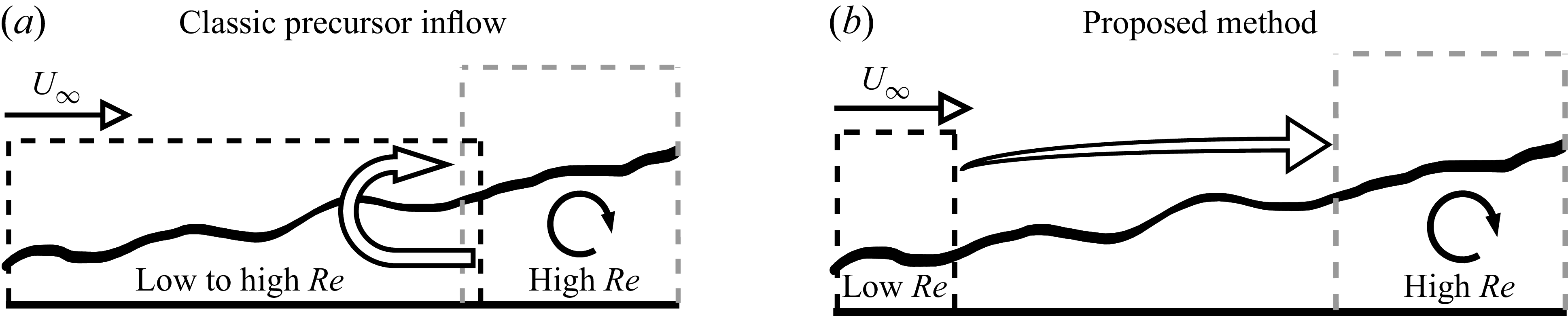
 Re
Re Re
Re Re
Re Re
Re
 kz
kz y
y kz=10
kz=10 Real{φ1(kz=10,n=0)}
 [±0.0015,±0.0030,±0.0045]
 z
z y
y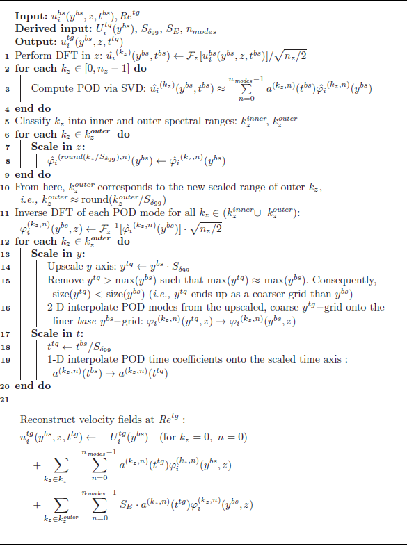
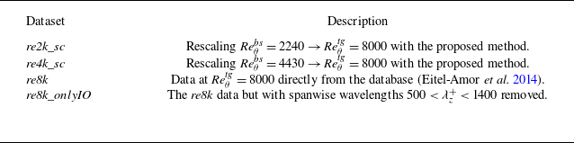

 u
u Euu+(kz)⋅kz
 u
u λz+
λz+ λt+
λt+ Euu+(ktkz)⋅ktkz
 y≈0.2δ990
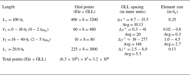
 Y1
Y1 Y2
Y2 Ly
Ly
 u
u Euu(kz)⋅kz/uτ2
 x=0θ0
x=0θ0 Reθ≈8000
 x=50θ0
 Reθ≈8500
 x=95θ0
 Reθ≈9000
 +
+ Re
Re
 Reθ=8700
 +
+
 cf
cf H12
H12 Reθ
Reθ cf
cf H12
H12 ±5%
±5% ±1%
±1% Reθ
Reθ Reθ
Reθ 0.3%
0.3% 1%
1%
 Open access

