





1 Introduction
The key technologies of all high-power lasers are chirped pulse amplification (CPA) or optical parametric chirped pulse amplification (OPCPA). Pulse stretching, amplification and compression inevitably lead to temporal contrast degradation, that is, to the formation of a pre-pulse long before the main pulse and the post-pulse after the main pulse. Contrast degradation occurs in a wide time interval from 100 fs to nanoseconds. The pre-pulse is hazardous, as the target may be destroyed before the arrival of the main pulse, which restrains laser application, especially in experiments with solid targets. Many causes of contrast degradation are of a temporal nature, so they may be analysed, as a rule, in the time domain. These include the amplified spontaneous emission from a seed laser and amplifiers (both laser and parametric), amplitude and phase distortions of the temporal spectrum of the pulse and residual reflections and nonlinearity of the refractive index[ Reference Li, Leng and Li 1 ]. A special case is light scattering on optical elements, which leads to the appearance of a noise field with a wide spatial spectrum. The propagation of such a field in a compressor or a stretcher leads to space–time coupling (see Refs. [Reference Dorrer2,Reference Jeandet, Jolly, Borot, Bussière, Dumont, Gautier, Gobert, Goddet, Gonsalves, Irman, Leemans, Lopez-Martens, Mennerat, Nakamura, Ouillé, Pariente, Pittman, Püschel, Sanson, Sylla, Thaury, Zeil and Quéré3] and references therein).
The physical reason for contrast degradation due to space–time coupling is the overtaking/lagging of the scattered pulse behind the main pulse. Lagging is the most frequent case. However, if one pair of gratings is located between the scatterer and the target (‘half’ of the compressor or stretcher), part of the scattered radiation overtakes the main pulse, resulting in the appearance of a pre-pulse. Since the time of overtaking is proportional to the spatial frequency, only small-scale fluctuations in the field amplitude or phase are significant for the contrast.
There are several reasons for scattering. First of all, it is an imperfect surface quality of the optical elements. The influence of imperfection on contrast was first numerically revealed in Ref. [Reference Bagnoud and Salin4]. Most subsequent works were devoted to numerical[
Reference Webb, Dorrer, Bahk, Jeon, Roides and Bromage
5
–
Reference Kiriyama, Mashiba, Miyasaka and Asakawa
13
] and experimental[
Reference Webb, Dorrer, Bahk, Jeon, Roides and Bromage
5
,
Reference Schanz, Roth and Bagnoud
8
,
Reference Li, Tokita, Matsuo, Sueda, Kurita, Kawasima and Miyanaga
10
–
Reference Zhu, Xie, Ouyang and Zhu
12
,
Reference Ranc, Blanc, Lebas, Martin, Zou, Mathieu, Radier, Ricaud, Druon and Papadopoulos
14
–
Reference Roeder, Zobus, Brabetz and Bagnoud
19
] studies of this effect both in the stretcher[
Reference Webb, Dorrer, Bahk, Jeon, Roides and Bromage
5
-
Reference Schanz, Roth and Bagnoud
8
,
Reference Li, Tokita, Matsuo, Sueda, Kurita, Kawasima and Miyanaga
10
–
Reference Roeder, Zobus, Brabetz and Bagnoud
19
] and in the compressor[
Reference Xie, Zhu, Zhu, Sun, Yang, Zhu, Guo, Kang and Gao
6
,
Reference Schanz, Roth and Bagnoud
8
–
Reference Kiriyama, Mashiba, Miyasaka and Asakawa
13
]. A theory without allowance for the diffraction and dispersion of a spatial chirp was proposed in Ref. [Reference Dorrer and Bromage20], developed in Ref. [Reference Bromage, Dorrer and Jungquist21], and later supplemented in Ref. [Reference Roeder, Zobus, Brabetz and Bagnoud19]. It was shown that the contrast is determined by the power spectral density (PSD) of the surface profile of the second and third gratings of stretcher/compressor and stretcher mirrors. These works are mainly focused on the intensity contrast in the far field, which is extremely difficult to measure. As a rule, the power contrast ratio (PCR) $\mathbb{C}(t)$
is measured as follows:
$\mathbb{C}(t)$
is measured as follows:
 $$\begin{align}\mathbb{C}(t)\equiv \frac{<{P}_\mathrm{out}(t)>-{P}_{0, \mathrm{out}}(t)}{P_{0, \mathrm{out}}(0)},\end{align}$$
where $<{P}_\mathrm{out}(t)>$
is the pulse power and
$<{P}_\mathrm{out}(t)>$
is the pulse power and ${P}_{0, \mathrm{out}}(t)$
is the power of the main pulse (neglecting the scattered field). Since the near and far fields are related by the spatial Fourier transform, then, according to Parseval’s theorem,
${P}_{0, \mathrm{out}}(t)$
is the power of the main pulse (neglecting the scattered field). Since the near and far fields are related by the spatial Fourier transform, then, according to Parseval’s theorem, $P(t)$
is the same in the near and far fields; consequently,
$P(t)$
is the same in the near and far fields; consequently, $\mathbb{C}(t)$
is also the same. Moreover, the analysis of Equation (13) from Ref. [Reference Bromage, Dorrer and Jungquist21] shows that in the near field the intensity contrast differs little from the power contrast. This means that the magnitude of
$\mathbb{C}(t)$
is also the same. Moreover, the analysis of Equation (13) from Ref. [Reference Bromage, Dorrer and Jungquist21] shows that in the near field the intensity contrast differs little from the power contrast. This means that the magnitude of $\mathbb{C}(t)$
is measured, even if the contrast meter covers only part of the aperture. Expressions for the PCR as a function of the PSD of the compressor/stretcher grating surface and the transport optics were obtained in Ref. [Reference Khazanov22] taking into account diffraction and all orders of dispersion.
$\mathbb{C}(t)$
is measured, even if the contrast meter covers only part of the aperture. Expressions for the PCR as a function of the PSD of the compressor/stretcher grating surface and the transport optics were obtained in Ref. [Reference Khazanov22] taking into account diffraction and all orders of dispersion.
At the same time, in addition to surface roughness, other optics imperfections whose influence has not been studied before also contribute to the PCR. First of all is the radiation scattering on dirt/damage/obscurations that inevitably appear both during the production of gratings and mirrors and in the course of their operation in high-power laser facilities[ Reference Spaeth, Manes, Widmayer, Williams, Whitman, Henesian, Stowers and Honig 23 ]. Following Ref. [Reference Spaeth, Manes, Widmayer, Williams, Whitman, Henesian, Stowers and Honig23], we will assume that the obscurations ‘absorb’ all incident laser light. Besides the roughness and obscurations of the beamline optics (gratings and mirrors), the roughness and obscurations of the mirrors used for writing holographic gratings also lead to degradation. They give rise to groove-shaped fluctuations leading to reflectivity fluctuations[ Reference Koch, Lehr and Glaser 24 ] as well as to non-equidistance and non-parallelism of the grooves, which in turn result in wave front fluctuations of diffracted radiation[ Reference Bienert, Röcker, Dietrich, Graf and Ahmed 25 – Reference Kochetkov, Shaykin, Yakovlev, Khazanov, Cheplakov, Wang, Jin, Liu and Shao 28 ]. In this work, we investigate in a general form the PCR caused by four reasons: roughness and obscurations of both beamline optics and writing optics. The only constraint that will be used is the spatial scale of obscurations and roughnesses and, hence, of the scattered radiation fluctuations much smaller than the beam diameter.
A general expression relating the PCR to the PSD of scattered field fluctuations is obtained in Section 2 without specifying the cause of scattering. Then, the PSD fields are found for obscurations of beamline optics (Section 3), for roughness of beamline optics (Section 4) and for obscurations and roughness of writing optics (Section 5). Section 6 provides an example of calculating the PCR using the obtained formulas and a discussion of the results.
2 General expression for the power contrast ratio $\mathbb{C}\left(\boldsymbol{t}\right)$

Most lasers use the Treacy compressor[
Reference Treacy
29
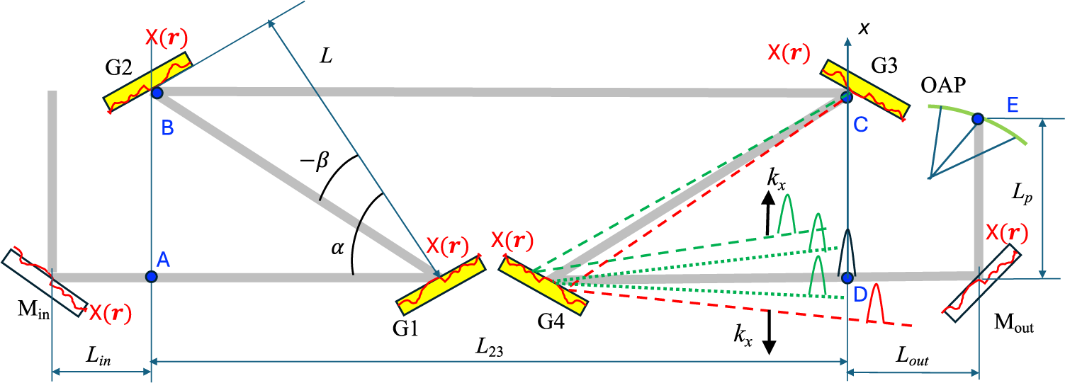
], shown in Figure 1, which has three parameters: $N$
is the groove density, L is the distance between the gratings along the normal and α is the angle of incidence on the first grating. In the general case of an out-of-plane compressor[
Reference Osvay and Ross
30
], there is one more parameter γ that is the angle of incidence on the first grating in the plane orthogonal to the diffraction plane. The angle of reflection
$N$
is the groove density, L is the distance between the gratings along the normal and α is the angle of incidence on the first grating. In the general case of an out-of-plane compressor[
Reference Osvay and Ross
30
], there is one more parameter γ that is the angle of incidence on the first grating in the plane orthogonal to the diffraction plane. The angle of reflection $\beta$
for the central frequency
$\beta$
for the central frequency ${\omega}_0=c{k}_0=2\pi c/{\lambda}_0$
is determined from the expression for the grating
${\omega}_0=c{k}_0=2\pi c/{\lambda}_0$
is determined from the expression for the grating $\sin\beta =-{\lambda}_0N/ \cos\gamma +\sin \alpha$
. An important special case of an out-of-plane compressor is the Littrow compressor[
Reference Khazanov
31
,
Reference Vyatkin and Khazanov
32
], in which
$\sin\beta =-{\lambda}_0N/ \cos\gamma +\sin \alpha$
. An important special case of an out-of-plane compressor is the Littrow compressor[
Reference Khazanov
31
,
Reference Vyatkin and Khazanov
32
], in which $\alpha ={\alpha}_\mathrm{L}$
, where
$\alpha ={\alpha}_\mathrm{L}$
, where ${\alpha}_\mathrm{L}$
is the Littrow angle. It is convenient to start the consideration with the field
${\alpha}_\mathrm{L}$
is the Littrow angle. It is convenient to start the consideration with the field ${E}_0\left(\Omega, \boldsymbol{r}\right)$
(
${E}_0\left(\Omega, \boldsymbol{r}\right)$
( $\Omega =\omega -{\omega}_0$
) incident on an imperfect optical element that may be any diffraction grating G1–G4 and input and output optics Min and Mout, as well as gratings and stretcher mirrors. We will search for the contrast
$\Omega =\omega -{\omega}_0$
) incident on an imperfect optical element that may be any diffraction grating G1–G4 and input and output optics Min and Mout, as well as gratings and stretcher mirrors. We will search for the contrast $\mathbb{C}(t)$
caused by each element separately, assuming that all other elements are perfect. After reflection, the field takes the following form:
$\mathbb{C}(t)$
caused by each element separately, assuming that all other elements are perfect. After reflection, the field takes the following form:
 $$\begin{align}{E}_1\left(\Omega, \boldsymbol{r}\right)={E}_0\left(\Omega, \boldsymbol{r}\right)+{E}_0\left(\Omega, \boldsymbol{r}\right)\left(\Theta \left(\boldsymbol{r}\right)+\mathcal{A}\left(\boldsymbol{r}\right)+ i\varphi \left(\boldsymbol{r}\right)\right),\end{align}$$
Compressor scheme. G1–G4, diffraction gratings; OAP, off-axis parabola; Min, input optics; Mout, output optics. Dotted lines represent radiation scattered by G4, where scattered pulses lag behind the main one. Dashed lines represent radiation scattered by G3, where scattered pulses lag behind (green) or overtake (red) the main pulse, depending on the sign of ${k}_x$
.
${k}_x$
.
where $\mathcal{A}\left(\boldsymbol{r}\right)\ll 1$
,
$\mathcal{A}\left(\boldsymbol{r}\right)\ll 1$
, $\varphi \left(\boldsymbol{r}\right)\ll 1$
and
$\varphi \left(\boldsymbol{r}\right)\ll 1$
and $\Theta \left(\boldsymbol{r}\right)$
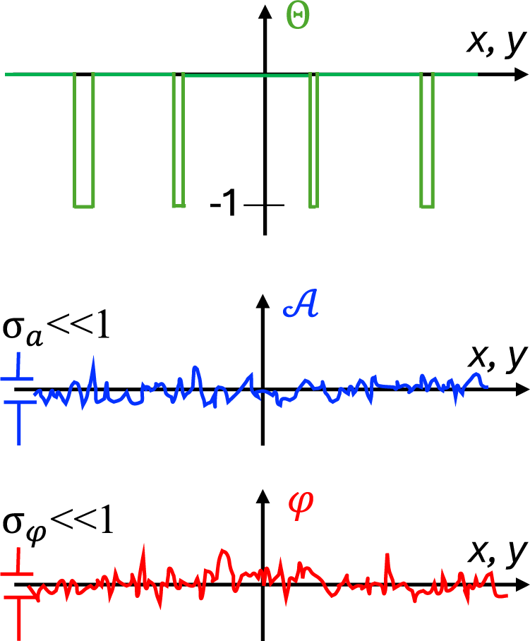
are real, homogeneous, ergodic random functions (fields) characterizing the fluctuations of the field amplitude and phase, as well as the presence of obscurations:
$\Theta \left(\boldsymbol{r}\right)$
are real, homogeneous, ergodic random functions (fields) characterizing the fluctuations of the field amplitude and phase, as well as the presence of obscurations: $\Theta \left(\boldsymbol{r}\right)=1$
inside and
$\Theta \left(\boldsymbol{r}\right)=1$
inside and $\Theta \left(\boldsymbol{r}\right)=0$
outside the obscurations. Following Ref. [Reference Spaeth, Manes, Widmayer, Williams, Whitman, Henesian, Stowers and Honig23], we assume that the obscurations ‘absorb’ all incident laser light, and thus they affect only the amplitude of the incident beam and not its phase. The size and coordinates of the obscurations on the surface of the optical element are random variables. The second term in Equation (2) will be further called noise for brevity, and the noise energy will be taken to be much lower than the energy of the main pulse
$\Theta \left(\boldsymbol{r}\right)=0$
outside the obscurations. Following Ref. [Reference Spaeth, Manes, Widmayer, Williams, Whitman, Henesian, Stowers and Honig23], we assume that the obscurations ‘absorb’ all incident laser light, and thus they affect only the amplitude of the incident beam and not its phase. The size and coordinates of the obscurations on the surface of the optical element are random variables. The second term in Equation (2) will be further called noise for brevity, and the noise energy will be taken to be much lower than the energy of the main pulse ${W}_0=\int {\left|{E}_0\left(\Omega, \boldsymbol{r}\right)\right|}^2\mathrm{d}\boldsymbol{r}\mathrm{d}\Omega$
:
${W}_0=\int {\left|{E}_0\left(\Omega, \boldsymbol{r}\right)\right|}^2\mathrm{d}\boldsymbol{r}\mathrm{d}\Omega$
:
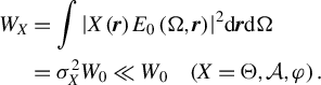 $$\begin{align}{W}_X&=\int {\left|X\left(\boldsymbol{r}\right){E}_0\left(\Omega, \boldsymbol{r}\right)\right|}^2\mathrm{d}\boldsymbol{r}\mathrm{d}\Omega\nonumber\\&={\sigma}_X^2{W}_0\ll {W}_0\kern0.84em \left(X=\Theta, \mathcal{A},\varphi \right).\end{align}$$
Since in this paper we are interested in small-scale intensity fluctuations, the characteristic spatial scale of ${E}_0\left(\boldsymbol{r}\right)$
is much larger than the characteristic spatial scale of
${E}_0\left(\boldsymbol{r}\right)$
is much larger than the characteristic spatial scale of $\Theta \left(\boldsymbol{r}\right)$
,
$\Theta \left(\boldsymbol{r}\right)$
, $\mathcal{A}\left(\boldsymbol{r}\right)$
and
$\mathcal{A}\left(\boldsymbol{r}\right)$
and $\varphi \left(\boldsymbol{r}\right)$
, that is, the correlation length of these functions is much smaller than the beam size. In other words, the spatial spectrum of the noise is much wider than the spectrum of the main beam. From ergodicity it follows that
$\varphi \left(\boldsymbol{r}\right)$
, that is, the correlation length of these functions is much smaller than the beam size. In other words, the spatial spectrum of the noise is much wider than the spectrum of the main beam. From ergodicity it follows that
 $$\begin{align}{\sigma}_X^2=<{X}^2\left(\boldsymbol{r}\right)>,\end{align}$$
with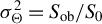 ${\sigma}_{\Theta}^2={S}_\mathrm{ob}/{S}_0$
, where
${\sigma}_{\Theta}^2={S}_\mathrm{ob}/{S}_0$
, where ${S}_\mathrm{ob}$
is the total area of all obscurations and
${S}_\mathrm{ob}$
is the total area of all obscurations and ${S}_0$
is the beam area. The angle brackets denote ensemble averaging. For clarity,
${S}_0$
is the beam area. The angle brackets denote ensemble averaging. For clarity, $\Theta \left(\boldsymbol{r}\right)$
,
$\Theta \left(\boldsymbol{r}\right)$
, $\mathcal{A}\left(\boldsymbol{r}\right)$
and
$\mathcal{A}\left(\boldsymbol{r}\right)$
and $\varphi \left(\boldsymbol{r}\right)$
are shown in Figure 2. Equation (2) has the most general form and includes all possible imperfections of the optical element. Note that beam clipping, which also affects the contrast[
Reference Khazanov
33
], is not described by Equation (2) and is outside the scope of this paper. The functions and their Fourier transforms will be designated by the same letters, but with different arguments:
$\varphi \left(\boldsymbol{r}\right)$
are shown in Figure 2. Equation (2) has the most general form and includes all possible imperfections of the optical element. Note that beam clipping, which also affects the contrast[
Reference Khazanov
33
], is not described by Equation (2) and is outside the scope of this paper. The functions and their Fourier transforms will be designated by the same letters, but with different arguments:
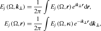 $$\begin{align}{E}_j\left(\Omega, \boldsymbol{k}_{\boldsymbol{\perp}} \right)&=\frac{1}{2\pi}\int {E}_j\left(\Omega, \boldsymbol{r}\right){e}^{i\boldsymbol{k}_{\boldsymbol{\perp}} \boldsymbol{r}}\mathrm{d}\boldsymbol{r},\nonumber\\{E}_j\left(\Omega, \boldsymbol{r}\right) &=\frac{1}{2\pi}\int {E}_j\left(\Omega, \boldsymbol{\kappa} \right){e}^{-i\boldsymbol{k}_{\boldsymbol{\perp}} \boldsymbol{r}}\mathrm{d}\boldsymbol{k}_{\boldsymbol{\perp}},\end{align}$$
Schematic representation of random functions $\Theta \left(\boldsymbol{r}\right),\ \mathcal{A}\left(\boldsymbol{r}\right)\mathrm{and}\;\varphi \left(\boldsymbol{r}\right)$
.
$\Theta \left(\boldsymbol{r}\right),\ \mathcal{A}\left(\boldsymbol{r}\right)\mathrm{and}\;\varphi \left(\boldsymbol{r}\right)$
.
and analogously for the temporal Fourier transform. Hereinafter, the range of integration, if not otherwise specified, is $\pm \infty$
. From Equations (2) and (5) we obtain the following:
$\pm \infty$
. From Equations (2) and (5) we obtain the following:
 $$\begin{align}{E}_1\left(\Omega, {\boldsymbol{k}}_{\boldsymbol{\perp}}\right)={E}_0\left(\Omega, {\boldsymbol{k}}_{\boldsymbol{\perp}}\right)-\frac{1}{2\pi}\int \mathrm{d}\boldsymbol{r}{e}^{i{\boldsymbol{k}}_{\boldsymbol{\perp}}\boldsymbol{r}}{E}_0\left(\Omega, \boldsymbol{r}\right)\mathcal{A}\left(\boldsymbol{r}\right).\end{align}$$
The field on the focusing parabola (point E in Figure 1) up to which the field ${E}_1\left(\Omega, {\boldsymbol{k}}_{\boldsymbol{\perp}}\right)$
in Equation (6) passes through an optical system containing a pair(s) of parallel gratings and a section(s) of free space of total length
${E}_1\left(\Omega, {\boldsymbol{k}}_{\boldsymbol{\perp}}\right)$
in Equation (6) passes through an optical system containing a pair(s) of parallel gratings and a section(s) of free space of total length ${L}_\mathrm{f}$
is considered to be the output field
${L}_\mathrm{f}$
is considered to be the output field ${E}_\mathrm{out}\left(\Omega, {\boldsymbol{k}}_{\boldsymbol{\perp}}\right).$
Regardless of the order in which these elements are passed, the field
${E}_\mathrm{out}\left(\Omega, {\boldsymbol{k}}_{\boldsymbol{\perp}}\right).$
Regardless of the order in which these elements are passed, the field ${E}_\mathrm{out}\left(\Omega, {\boldsymbol{k}}_{\boldsymbol{\perp}}\right)$
has the following form:
${E}_\mathrm{out}\left(\Omega, {\boldsymbol{k}}_{\boldsymbol{\perp}}\right)$
has the following form:
 $$\begin{align}{E}_\mathrm{out}\left(\Omega, {\boldsymbol{k}}_{\boldsymbol{\perp}}\right)={E}_1\left(\Omega, {\boldsymbol{k}}_{\boldsymbol{\perp}}\right){e}^{i\Psi \left(\Omega, {\boldsymbol{k}}_{\boldsymbol{\perp}}\right)},\end{align}$$
where $\Psi \left(\Omega, {\boldsymbol{k}}_{\boldsymbol{\perp}}\right)$
is the sum of the phase
$\Psi \left(\Omega, {\boldsymbol{k}}_{\boldsymbol{\perp}}\right)$
is the sum of the phase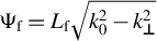 ${\Psi}_\mathrm{f}={L}_\mathrm{f}\sqrt{k_0^2-{k}_{\boldsymbol{\perp}}^2}$
introduced by the free space of length
${\Psi}_\mathrm{f}={L}_\mathrm{f}\sqrt{k_0^2-{k}_{\boldsymbol{\perp}}^2}$
introduced by the free space of length ${L}_\mathrm{f}$
and (i) by two pairs of parallel diffraction gratings from point A to point B and from point C to point D for Min or G1; or (ii) by one pair from point C to point D for G2 or G3; or (iii) there are no other terms for G4 or Mout. It is convenient to present the function
${L}_\mathrm{f}$
and (i) by two pairs of parallel diffraction gratings from point A to point B and from point C to point D for Min or G1; or (ii) by one pair from point C to point D for G2 or G3; or (iii) there are no other terms for G4 or Mout. It is convenient to present the function $\Psi \left(\Omega, {\boldsymbol{k}}_{\boldsymbol{\perp}}\right)$
as a Taylor series at the point
$\Psi \left(\Omega, {\boldsymbol{k}}_{\boldsymbol{\perp}}\right)$
as a Taylor series at the point $\Omega =0$
,
$\Omega =0$
, ${k}_x={k}_y=0$
(
${k}_x={k}_y=0$
( ${k}_{x,y}$
are the components of the vector
${k}_{x,y}$
are the components of the vector ${\boldsymbol{k}}_{\boldsymbol{\perp}}$
) by extracting the term of the first power in
${\boldsymbol{k}}_{\boldsymbol{\perp}}$
) by extracting the term of the first power in $\Omega$
and designating all the other terms as
$\Omega$
and designating all the other terms as $\Phi \left(\Omega, {\boldsymbol{k}}_{\boldsymbol{\perp}}\right)$
:
$\Phi \left(\Omega, {\boldsymbol{k}}_{\boldsymbol{\perp}}\right)$
:
 $$\begin{align}\Psi \left(\Omega, {\boldsymbol{k}}_{\boldsymbol{\perp}}\right)=\Omega \tau \left({\boldsymbol{k}}_{\boldsymbol{\perp}}\right)+\Phi \left(\Omega, {\boldsymbol{k}}_{\boldsymbol{\perp}}\right).\end{align}$$
The expressions for the phase introduced by the pair of parallel diffraction gratings ${\Psi}_\mathrm{p}\left(\Omega, {\boldsymbol{k}}_{\boldsymbol{\perp}}\right)$
, as well as for
${\Psi}_\mathrm{p}\left(\Omega, {\boldsymbol{k}}_{\boldsymbol{\perp}}\right)$
, as well as for ${\psi}_\mathrm{a}^b$
derivatives of
${\psi}_\mathrm{a}^b$
derivatives of ${\Psi}_\mathrm{p}$
with respect to
${\Psi}_\mathrm{p}$
with respect to $\omega$
,
$\omega$
, ${k}_x$
,
${k}_x$
, ${k}_y$
at the point
${k}_y$
at the point $\Omega =0$
,
$\Omega =0$
, ${k}_x={k}_y=0$
, also needed for the Taylor series, can be found in Refs. [Reference Khazanov34,Reference Kocharovskaya, Martyanov and Khazanov35]. Using them, one can obtain the expression for
${k}_x={k}_y=0$
, also needed for the Taylor series, can be found in Refs. [Reference Khazanov34,Reference Kocharovskaya, Martyanov and Khazanov35]. Using them, one can obtain the expression for $\tau \left({\boldsymbol{k}}_{\boldsymbol{\perp}}\right)$
in the following form:
$\tau \left({\boldsymbol{k}}_{\boldsymbol{\perp}}\right)$
in the following form:
 $$\begin{align}\tau \left({\boldsymbol{k}}_{\boldsymbol{\perp}}\right)&=2{\tau}_x\frac{k_x}{k_0}+2{\tau}_y\frac{k_y}{k_0}+{t}_x\frac{k_x^2}{k_0^2}+{t}_y\frac{k_y^2}{k_0^2}+2{t}_{xy}\frac{k_x{k}_y}{k_0^2},\end{align}$$
 $$\begin{align}{\tau}_x&=\frac{1}{2}{k}_0{\psi}_{x\omega}^{\prime \prime }=\mp \frac{AL}{2c},\kern1.92em {\tau}_y=\frac{1}{2}{k}_0{\psi}_{y\omega}^{\prime \prime }=\mp \frac{GL}{2c},\end{align}$$
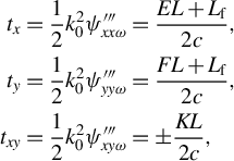 $$\begin{align}{t}_x&=\frac{1}{2}{k}_0^2{\psi}_{xx\omega}^{\prime \prime \prime }=\frac{EL+{L}_\mathrm{f}}{2c},\nonumber\\{t}_y&=\frac{1}{2}{k}_0^2{\psi}_{yy\omega}^{\prime \prime \prime }=\frac{FL+{L}_\mathrm{f}}{2c},\nonumber\\{t}_{xy}&=\frac{1}{2}{k}_0^2{\psi}_{xy\omega}^{\prime \prime \prime }=\pm \frac{KL}{2c},\end{align}$$
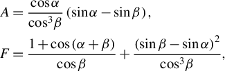 $$\begin{align}A&=\frac{\cos\alpha}{{\mathit{\cos}}^3\beta}\left( \sin\alpha - \sin\beta \right),\kern0.72em\nonumber\\ F&=\frac{1+\cos \left(\alpha +\beta \right)}{\cos\beta}+\frac{{\left( \sin\beta - \sin\alpha \right)}^2}{{\mathit{\cos}}^3\beta },\end{align}$$
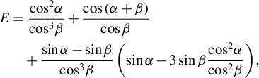 $$\begin{align}E&=\frac{{\mathit{\cos}}^2\alpha }{{\mathit{\cos}}^3\beta }+\frac{\cos \left(\alpha +\beta \right)}{\cos\beta}\nonumber\\&\quad+\frac{\sin\alpha - \sin\beta}{{\mathit{\cos}}^3\beta}\left( \sin\alpha -3 \sin\beta \frac{{\mathit{\cos}}^2\alpha }{{\mathit{\cos}}^2\beta}\right),\end{align}$$
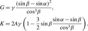 $$\begin{align}G&=\gamma \frac{{\left( \sin\beta - \sin\alpha \right)}^2}{{\mathit{\cos}}^3\beta},\nonumber\\K&=2 A\gamma \left(1-\frac{3}{2} \sin\beta \frac{\sin\alpha - \sin\beta}{{\mathit{\cos}}^3\beta}\right).\end{align}$$
As $\gamma \ll 1$
in the general case, terms of order
$\gamma \ll 1$
in the general case, terms of order ${\gamma}^2$
are omitted here. From here on we will restrict ourselves to the paraxial approximation, that is, we will consider
${\gamma}^2$
are omitted here. From here on we will restrict ourselves to the paraxial approximation, that is, we will consider ${k}_{x,y}$
of powers not higher than 2. Thus, we take into account diffraction in the paraxial approximation and all orders of dispersion, including the dispersion of the spatial chirp, since the term
${k}_{x,y}$
of powers not higher than 2. Thus, we take into account diffraction in the paraxial approximation and all orders of dispersion, including the dispersion of the spatial chirp, since the term $\Phi \left(\Omega, {\boldsymbol{k}}_{\boldsymbol{\perp}}\right)$
includes terms with
$\Phi \left(\Omega, {\boldsymbol{k}}_{\boldsymbol{\perp}}\right)$
includes terms with ${\Omega}^2$
,
${\Omega}^2$
, ${\Omega}^3$
, etc. Further, we assume that the grating pairs in the compressor are identical. This is not the case for an asymmetric compressor[
Reference Khazanov
34
,
Reference Huang and Kessler
36
–
Reference Liang, Du, Chen, Wang, Liu, Chen, Shena, Liu and Li
42
], but we restrict consideration to a symmetric one. The sign ∓ in Equations (10) and (11) corresponds to the first and second pairs of gratings; therefore, for two pairs of gratings, the total values of
${\Omega}^3$
, etc. Further, we assume that the grating pairs in the compressor are identical. This is not the case for an asymmetric compressor[
Reference Khazanov
34
,
Reference Huang and Kessler
36
–
Reference Liang, Du, Chen, Wang, Liu, Chen, Shena, Liu and Li
42
], but we restrict consideration to a symmetric one. The sign ∓ in Equations (10) and (11) corresponds to the first and second pairs of gratings; therefore, for two pairs of gratings, the total values of ${t}_{xx}$
,
${t}_{xx}$
, ${t}_{yy}$
are doubled, and
${t}_{yy}$
are doubled, and ${\tau}_x={\tau}_y={t}_{xy}=0.$
Note that, if α is equal to the Littrow angle, then
${\tau}_x={\tau}_y={t}_{xy}=0.$
Note that, if α is equal to the Littrow angle, then $F=E$
. This is not the case for the Treacy compressor, but usually α is chosen as close to the Littrow angle as the decoupling condition allows (the beam incident on grating G1 should not overlap with the second grating). Hence, for the compressor, the values of F and E are close, for example, in the XCELS project[
Reference Khazanov, Shaykin, Kostyukov, Ginzburg, Mukhin, Yakovlev, Soloviev, Kuznetsov, Mironov, Korzhimanov, Bulanov, Shaikin, Kochetkov, Kuzmin, Martyanov, Lozhkarev, Starodubtsev, Litvak and Sergeev
43
]
$F=E$
. This is not the case for the Treacy compressor, but usually α is chosen as close to the Littrow angle as the decoupling condition allows (the beam incident on grating G1 should not overlap with the second grating). Hence, for the compressor, the values of F and E are close, for example, in the XCELS project[
Reference Khazanov, Shaykin, Kostyukov, Ginzburg, Mukhin, Yakovlev, Soloviev, Kuznetsov, Mironov, Korzhimanov, Bulanov, Shaikin, Kochetkov, Kuzmin, Martyanov, Lozhkarev, Starodubtsev, Litvak and Sergeev
43
] $F=1.025E$
and we can assume that
$F=1.025E$
and we can assume that ${\tau}_y\approx {\tau}_x$
. This condition is fulfilled exactly for the Littrow compressor[
Reference Khazanov
31
,
Reference Vyatkin and Khazanov
32
].
${\tau}_y\approx {\tau}_x$
. This condition is fulfilled exactly for the Littrow compressor[
Reference Khazanov
31
,
Reference Vyatkin and Khazanov
32
].
The quantity $\tau \left({\boldsymbol{k}}_{\boldsymbol{\perp}}\right)$
has a simple physical meaning – it is the time delay of the noise component with wave vector
$\tau \left({\boldsymbol{k}}_{\boldsymbol{\perp}}\right)$
has a simple physical meaning – it is the time delay of the noise component with wave vector ${\boldsymbol{k}}_{\boldsymbol{\perp}}$
relative to the wave with
${\boldsymbol{k}}_{\boldsymbol{\perp}}$
relative to the wave with ${\boldsymbol{k}}_{\boldsymbol{\perp}}=0$
. Since
${\boldsymbol{k}}_{\boldsymbol{\perp}}=0$
. Since $E>0$
and
$E>0$
and $EF>{K}^2$
, the last three terms in Equation (9) are a positively defined quadratic form, that is, the only negative terms in Equation (9) are the terms with
$EF>{K}^2$
, the last three terms in Equation (9) are a positively defined quadratic form, that is, the only negative terms in Equation (9) are the terms with ${\tau}_x$
and
${\tau}_x$
and ${\tau}_y$
. If
${\tau}_y$
. If ${\tau}_x={\tau}_y=0$
, then all noise components lag behind the main wave, which means that at
${\tau}_x={\tau}_y=0$
, then all noise components lag behind the main wave, which means that at $t<0$
the contrast is zero (a perfect case). This is true for all optical elements in Figure 1, except for gratings G2 and G3.
$t<0$
the contrast is zero (a perfect case). This is true for all optical elements in Figure 1, except for gratings G2 and G3.
The power ${P}_\mathrm{out}(t)$
required for calculating
${P}_\mathrm{out}(t)$
required for calculating $\mathbb{C}(t)$
by the definition in Equation (1) is as follows:
$\mathbb{C}(t)$
by the definition in Equation (1) is as follows:
 $$\begin{align}{P}_\mathrm{out}(t)=\int {\left|{E}_\mathrm{out}\left(t,{\boldsymbol{k}}_{\boldsymbol{\perp}}\right)\right|}^2\mathrm{d}{\boldsymbol{k}}_{\boldsymbol{\perp}}.\end{align}$$
By substituting Equation (8) into Equation (7) and performing the inverse time Fourier transform we obtain ${E}_\mathrm{out}\left(t,{\boldsymbol{k}}_{\boldsymbol{\perp}}\right)$
. By substituting it into Equation (15) and the result into Equation (1) we find
${E}_\mathrm{out}\left(t,{\boldsymbol{k}}_{\boldsymbol{\perp}}\right)$
. By substituting it into Equation (15) and the result into Equation (1) we find $\mathbb{C}(t)$
. The transformations absolutely analogous to Ref. [Reference Khazanov22] yield the following:
$\mathbb{C}(t)$
. The transformations absolutely analogous to Ref. [Reference Khazanov22] yield the following:
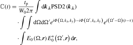 $$\begin{align}\mathbb{C}(t)&=\frac{t_\mathrm{p}}{W_02\pi}\int \mathrm{d}{\boldsymbol{k}}_{\boldsymbol{\perp}} \mathrm{PSD2}\left({\boldsymbol{k}}_{\boldsymbol{\perp}}\right)\nonumber\\&\quad\cdot\int \int \mathrm{d}\Omega \mathrm{d}\Omega^{\prime }{e}^{i\varPhi \left(\Omega, {k}_x,{k}_y\right)- i\varPhi \left({\Omega}^{\prime}, {k}_x,{k}_y\right)}{e}^{i\left({\Omega}^{\prime }-\Omega \right)\left(t-\tau \right)}\nonumber\\&\quad\cdot\int {E}_0\left(\Omega, \boldsymbol{r}\right){E}_0^{\ast}\left(\Omega^{\prime },\boldsymbol{r}\right)\mathrm{d}\boldsymbol{r},\kern0.48em\end{align}$$
where ${t}_\mathrm{p}={W}_0/{P}_{0, \mathrm{out}}(0)$
is the duration of the output pulse and
${t}_\mathrm{p}={W}_0/{P}_{0, \mathrm{out}}(0)$
is the duration of the output pulse and
 $$\begin{align}\mathrm{PSD}2\left({\boldsymbol{k}}_{\boldsymbol{\perp}}\right)= \mathrm{PSD}{2}_{\Theta}\left({\boldsymbol{k}}_{\boldsymbol{\perp}}\right)+ \mathrm{PSD}{2}_{\mathcal{A}}\left({\boldsymbol{k}}_{\boldsymbol{\perp}}\right)+ \mathrm{PSD}{2}_{\varphi}\left({\boldsymbol{k}}_{\boldsymbol{\perp}}\right),\end{align}$$
where $\mathrm{PSD}{2}_X\left({\boldsymbol{k}}_{\boldsymbol{\perp}}\right)$
is the two-dimensional PSD of the function
$\mathrm{PSD}{2}_X\left({\boldsymbol{k}}_{\boldsymbol{\perp}}\right)$
is the two-dimensional PSD of the function $X$
$X$ $\left(X=\Theta, \mathcal{A},\varphi \right)$
defined by the following:
$\left(X=\Theta, \mathcal{A},\varphi \right)$
defined by the following:
 $$\begin{align}\mathrm{PSD}{2}_X\left({\boldsymbol{k}}_{\boldsymbol{\perp}}\right)={\left(2\pi \right)}^2\int \mathrm{ACF}_X\left(\boldsymbol{\rho} \right){e}^{i{\boldsymbol{k}}_{\boldsymbol{\perp}}\boldsymbol{\rho}}\mathrm{d}\boldsymbol{\rho },\end{align}$$
where $\mathrm{ACF}_X\left(\boldsymbol{\rho} \right)=<X\left(\boldsymbol{r}-\boldsymbol{\rho} \right)X\left(\boldsymbol{r}\right)>$
. Here we took into account that
$\mathrm{ACF}_X\left(\boldsymbol{\rho} \right)=<X\left(\boldsymbol{r}-\boldsymbol{\rho} \right)X\left(\boldsymbol{r}\right)>$
. Here we took into account that $\Theta \left(\boldsymbol{r}\right)$
,
$\Theta \left(\boldsymbol{r}\right)$
, $\mathcal{A}\left(\boldsymbol{r}\right)$
and
$\mathcal{A}\left(\boldsymbol{r}\right)$
and $\varphi \left(\boldsymbol{r}\right)$
are uncorrelated with each other. Note that the noise energy is, evidently,
$\varphi \left(\boldsymbol{r}\right)$
are uncorrelated with each other. Note that the noise energy is, evidently, ${W}_{\mathrm{n}}={P}_{0, \mathrm{out}}(0)\int \mathbb{C}(t) \mathrm{d}t={W}_{\Theta}+{W}_{\mathcal{A}}+{W}_{\varphi }$
. The integration of Equation (16) with respect to
${W}_{\mathrm{n}}={P}_{0, \mathrm{out}}(0)\int \mathbb{C}(t) \mathrm{d}t={W}_{\Theta}+{W}_{\mathcal{A}}+{W}_{\varphi }$
. The integration of Equation (16) with respect to $t$
gives
$t$
gives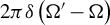 $2\pi \delta \left({\Omega}^{\prime }-\Omega \right)$
, where
$2\pi \delta \left({\Omega}^{\prime }-\Omega \right)$
, where $\delta$
is the Dirac delta function. Next, taking into account Equation (3) we obtain an obvious relation:
$\delta$
is the Dirac delta function. Next, taking into account Equation (3) we obtain an obvious relation:
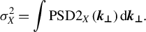 $$\begin{align}{\sigma}_X^2=\int \mathrm{PSD}{2}_X\left({\boldsymbol{k}}_{\boldsymbol{\perp}}\right)\mathrm{d}{\boldsymbol{k}}_{\boldsymbol{\perp}}.\end{align}$$
The $\mathrm{PSD}2$
definition in Equation (18) is known in the literature, but it is not the only one. It differs from the definition used, for example, in Refs. [Reference Bromage, Dorrer and Jungquist21,Reference Khazanov22,Reference Martyanov and Khazanov44], where there is no
$\mathrm{PSD}2$
definition in Equation (18) is known in the literature, but it is not the only one. It differs from the definition used, for example, in Refs. [Reference Bromage, Dorrer and Jungquist21,Reference Khazanov22,Reference Martyanov and Khazanov44], where there is no ${\left(2\pi \right)}^2$
multiplier. We chose that in Equation (18), since in this case Equation (19) for
${\left(2\pi \right)}^2$
multiplier. We chose that in Equation (18), since in this case Equation (19) for ${\sigma}_X^2$
has a simpler form. In the special case of pure phase distortions
${\sigma}_X^2$
has a simpler form. In the special case of pure phase distortions $\left(\mathcal{A}=\Theta =0\right),$
Equation (16) coincides with Equation (14) from Ref. [Reference Khazanov22].
$\left(\mathcal{A}=\Theta =0\right),$
Equation (16) coincides with Equation (14) from Ref. [Reference Khazanov22].
By substituting Equation (11) into Equation (16) we change the variables:
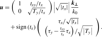 $$\begin{align}\boldsymbol{u}&=\left(\begin{array}{cc}1& {t}_{xy}/{t}_x\\ {}0& \sqrt{T_y/{t}_x}\end{array}\right)\left|\sqrt{\left|{t}_x\right|}\right|\frac{{\boldsymbol{k}}_{\boldsymbol{\perp}}}{k_0}\nonumber\\&\quad+\mathit{\operatorname{sign}}\left({t}_x\right)\left(\begin{array}{c}{\tau}_x/\sqrt{\left|{t}_x\right|}\\ {}\left({\tau}_y-\frac{t_{xy}}{t_x}{\tau}_x\right)/\sqrt{\left|{T}_y\right|}\end{array}\right).\end{align}$$
Further, supposing that $\mathrm{PSD}2$
is an isotropic function, that is,
$\mathrm{PSD}2$
is an isotropic function, that is, $\mathrm{PSD}2\left({k}_x,{k}_y\right)= \mathrm{PSD}2\left({k}_{\perp}\right)$
and passing from
$\mathrm{PSD}2\left({k}_x,{k}_y\right)= \mathrm{PSD}2\left({k}_{\perp}\right)$
and passing from $\left({u}_x,{u}_y\right)$
to the polar coordinates
$\left({u}_x,{u}_y\right)$
to the polar coordinates $\left(u,\theta \right)$
, we obtain
$\left(u,\theta \right)$
, we obtain
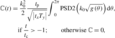 $$\begin{align}\mathbb{C}(t)&=\frac{k_0^2}{2}\frac{t_\mathrm{p}}{\sqrt{\left|{t}_x{T}_y\right|}}{\int}_0^{2\pi } \mathrm{PSD}2\left({k}_0\sqrt{g\left(\theta \right)}\right) \mathrm{d}\theta, \nonumber\\&\quad \mathrm{if}\;\frac{t}{t_\mathrm{c}}>-1;\qquad\mathrm{otherwise}\;\mathbb{C}=0,\end{align}$$
where
 $$\begin{align}{t}_\mathrm{c}=\frac{1}{T_y{t}_x}\left({t}_y{\tau}_x^2+{t}_x{\tau}_y^2-2{t}_{xy}{\tau}_y{\tau}_x\right),\end{align}$$
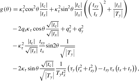 $$\begin{align}g\left(\theta \right)&={\kappa}_{\tau}^2{\mathit{\cos}}^2\theta \frac{\left|{t}_\mathrm{c}\right|}{\left|{t}_x\right|}+{\kappa}_{\tau}^2{\mathit{\sin}}^2\theta \frac{\left|{t}_\mathrm{c}\right|}{\left|{t}_x\right|}\left({\left(\frac{t_{xy}}{t_x}\right)}^2+\frac{\left|{t}_x\right|}{\left|{T}_y\right|}\right)\nonumber\\&-2{q}_x{\kappa}_{\tau } \cos\theta \frac{\sqrt{\left|{t}_\mathrm{c}\right|}}{\sqrt{\left|{t}_x\right|}}+{q}_x^2+{q}_y^2\nonumber\\&-{\kappa}_{\tau}^2\frac{\left|{t}_\mathrm{c}\right|}{\sqrt{\left|{t}_x\right|}}\frac{t_{xy}}{t_x}\mathit{\sin}2\theta \frac{1}{\sqrt{\left|{T}_y\right|}}\nonumber\\&-2{\kappa}_{\tau } \sin\theta \frac{\sqrt{\left|{t}_\mathrm{c}\right|}}{\sqrt{\left|{T}_y\right|}}\frac{1}{T_y{t}_x^2}\left({\tau}_y\left({t}_x^2+{t}_{xy}^2\right)-{t}_{xy}{\tau}_x\left({t}_x+{t}_y\right)\right),\end{align}$$
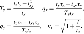 $$\begin{align}{T}_y&=\frac{t_x{t}_y-{t}_{xy}^2}{t_x},\kern0.96em {q}_x=\frac{t_y{\tau}_x-{t}_{xy}{\tau}_y}{T_y{t}_x},\nonumber\\{q}_y&=\frac{t_x{\tau}_y-{t}_{xy}{\tau}_x}{T_y{t}_x},\kern0.84em {\kappa}_{\tau }=\sqrt{1+\frac{t}{t_\mathrm{c}}}.\end{align}$$
Here we restrict consideration to the case ${t}_x{t}_y>0$
(the diffraction has the same sign along х and у), which is always fulfilled for the compressor, but not always for the stretcher[
Reference Khazanov
22
], and take into account that
${t}_x{t}_y>0$
(the diffraction has the same sign along х and у), which is always fulfilled for the compressor, but not always for the stretcher[
Reference Khazanov
22
], and take into account that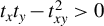 ${t}_x{t}_y-{t}_{xy}^2>0$
(i.e.,
${t}_x{t}_y-{t}_{xy}^2>0$
(i.e., ${T}_y$
has the same sign as
${T}_y$
has the same sign as ${t}_x$
). Note that only
${t}_x$
). Note that only ${\kappa}_{\tau }$
is time dependent.
${\kappa}_{\tau }$
is time dependent.
Next, we take into account that $\gamma \ll 1$
and, consequently,
$\gamma \ll 1$
and, consequently, $\frac{t_{xy}}{t_x}\sim \gamma \ll 1$
and
$\frac{t_{xy}}{t_x}\sim \gamma \ll 1$
and $\frac{\tau_y}{t_x}\sim \gamma \ll 1$
. By expanding
$\frac{\tau_y}{t_x}\sim \gamma \ll 1$
. By expanding $\mathbb{C}\left(t,\gamma \right)$
in a Taylor series near the point
$\mathbb{C}\left(t,\gamma \right)$
in a Taylor series near the point $\gamma =0$
it is easy to show that the term proportional to
$\gamma =0$
it is easy to show that the term proportional to $\gamma$
vanishes. Consequently, the difference in the contrast
$\gamma$
vanishes. Consequently, the difference in the contrast $\mathbb{C}\left(t,\gamma \right)$
for an out-of-plane compressor from the contrast
$\mathbb{C}\left(t,\gamma \right)$
for an out-of-plane compressor from the contrast $\mathbb{C}\left(t,\gamma =0\right)$
for a plane compressor reduces to corrections of the order of
$\mathbb{C}\left(t,\gamma =0\right)$
for a plane compressor reduces to corrections of the order of ${\gamma}^2$
. For typical values of
${\gamma}^2$
. For typical values of $\gamma =10,\dots, 15$
degrees, the correction will be about 5%, which is negligibly small for contrast. Thus, PCR
$\gamma =10,\dots, 15$
degrees, the correction will be about 5%, which is negligibly small for contrast. Thus, PCR $\mathbb{C}(t)$
does not depend on γ and we can use the expressions for a plane compressor. In other words, the contrast of an out-of-plane compressor practically does not differ from the contrast of a plane one. At
$\mathbb{C}(t)$
does not depend on γ and we can use the expressions for a plane compressor. In other words, the contrast of an out-of-plane compressor practically does not differ from the contrast of a plane one. At $\gamma =0,$
Equation (21) strictly passes into Equation (19) from Ref. [Reference Khazanov22] (taking into consideration that the definition of
$\gamma =0,$
Equation (21) strictly passes into Equation (19) from Ref. [Reference Khazanov22] (taking into consideration that the definition of $\mathrm{PSD}2$
in Ref. [Reference Khazanov22] differs from Equation (18) by the multiplier
$\mathrm{PSD}2$
in Ref. [Reference Khazanov22] differs from Equation (18) by the multiplier ${\left(2\pi \right)}^2$
). Therefore, the results obtained in Ref. [Reference Khazanov22] for phase noise are valid in the general case if
${\left(2\pi \right)}^2$
). Therefore, the results obtained in Ref. [Reference Khazanov22] for phase noise are valid in the general case if $\mathrm{PSD}{2}_{\varphi}\left({\boldsymbol{k}}_{\boldsymbol{\perp}}\right)$
is replaced by
$\mathrm{PSD}{2}_{\varphi}\left({\boldsymbol{k}}_{\boldsymbol{\perp}}\right)$
is replaced by $\mathrm{PSD}2\left({\boldsymbol{k}}_{\boldsymbol{\perp}}\right)$
in Equation (17). In particular, if we take into account that
$\mathrm{PSD}2\left({\boldsymbol{k}}_{\boldsymbol{\perp}}\right)$
in Equation (17). In particular, if we take into account that ${t}_x\approx {t}_y={t}_\mathrm{d}$
, then Equation (21) takes the following form:
${t}_x\approx {t}_y={t}_\mathrm{d}$
, then Equation (21) takes the following form:
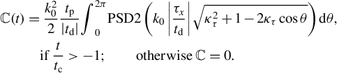 $$\begin{align}\mathbb{C}(t)&=\frac{k_0^2}{2}\frac{t_\mathrm{p}}{\left|{t}_\mathrm{d}\right|}{\int}_0^{2\pi } \mathrm{PSD}2\left({k}_0\left|\frac{\tau_x}{t_\mathrm{d}}\right|\sqrt{\kappa_{\tau}^2+1-2{\kappa}_{\tau } \cos\theta}\right) \mathrm{d}\theta,\nonumber\\&\quad \mathrm{if}\;\frac{t}{t_\mathrm{c}}>-1;\qquad\mathrm{otherwise}\;\mathbb{C}=0.\end{align}$$
This expression is significantly simplified in two important particular cases. Firstly, for G2 and G3 gratings, the allowance for diffraction $\left({t}_\mathrm{d}\ne 0\right)$
leads to the emergence of the cut-off time
$\left({t}_\mathrm{d}\ne 0\right)$
leads to the emergence of the cut-off time ${t}_\mathrm{c}$
and to a slight contrast asymmetry, which can be neglected, then
${t}_\mathrm{c}$
and to a slight contrast asymmetry, which can be neglected, then
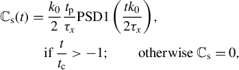 $$\begin{align}{\mathbb{C}}_\mathrm{s}(t)&=\frac{k_0}{2}\frac{t_\mathrm{p}}{\tau_x} \mathrm{PSD}1\left(\frac{t{k}_0}{2{\tau}_x}\right),\nonumber\\& \quad \mathrm{if}\;\frac{t}{t_\mathrm{c}}>-1; \qquad \mathrm{otherwise}\;{\mathbb{C}}_\mathrm{s}=0,\end{align}$$
where $\mathrm{PSD}1\left({k}_x\right)$
is a one-dimensional PSD function related to
$\mathrm{PSD}1\left({k}_x\right)$
is a one-dimensional PSD function related to $\mathrm{PSD}2\left({k}_{\perp}\right)$
as follows[
Reference Khazanov, Kochetkov and Silin
45
]:
$\mathrm{PSD}2\left({k}_{\perp}\right)$
as follows[
Reference Khazanov, Kochetkov and Silin
45
]:
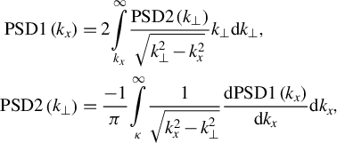 $$\begin{align}\mathrm{PSD}1\left({k}_x\right)&=2\underset{k_x}{\overset{\infty }{\int }}\frac{\mathrm{PSD}2\left({k}_{\perp}\right)}{\sqrt{k_{\perp}^2-{k}_x^2}}{k}_{\perp }\mathrm{d}{k}_{\perp},\nonumber\\\mathrm{PSD}2\left({k}_{\perp}\right)&=\frac{-1}{\pi}\underset{\kappa }{\overset{\infty }{\int }}\frac{1}{\sqrt{k_x^2-{k}_{\perp}^2}}\frac{\mathrm{d}\mathrm{PSD}1\left({k}_x\right)}{\mathrm{d}{k}_x}\mathrm{d}{k}_x,\end{align}$$
with
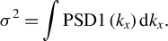 $$\begin{align}{\sigma}^2=\int \mathrm{PSD}1\left({k}_x\right)\mathrm{d}{k}_x.\end{align}$$
Secondly, there is no space chirp ${\tau}_x={\tau}_y=0$
for all optical elements in Figure 1, except for gratings G2 and G3; for them, the contrast
${\tau}_x={\tau}_y=0$
for all optical elements in Figure 1, except for gratings G2 and G3; for them, the contrast ${\mathbb{C}}_\mathrm{d}(t)$
is determined only by the diffraction:
${\mathbb{C}}_\mathrm{d}(t)$
is determined only by the diffraction:
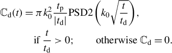 $$\begin{align}{\mathbb{C}}_\mathrm{d}(t)&=\pi {k}_0^2\frac{t_\mathrm{p}}{\left|{t}_\mathrm{d}\right|} \mathrm{PSD}2\left({k}_0\sqrt{\frac{t}{t_\mathrm{d}}}\right),\kern0.24em \nonumber\\& \quad \mathrm{if}\;\frac{t}{t_\mathrm{d}}>0;\qquad \mathrm{otherwise}\;{\mathbb{C}}_\mathrm{d}=0.\end{align}$$
If ${t}_\mathrm{d}>0$
, then
${t}_\mathrm{d}>0$
, then ${\mathbb{C}}_\mathrm{d}\left(t<0\right)=0$
, which explains the frequently observed[
Reference Webb, Dorrer, Bahk, Jeon, Roides and Bromage
5
,
Reference Hooker, Tang, Chekhlov, Collier, Divall, Ertel, Hawkes, Parry and Rajeev
15
–
Reference Lu, Zhang, Li and Leng
18
,
Reference Wang, Liu, Lu, Chen, Long, Li, Chen, Chen, Bai, Li, Peng, Liu, Wu, Wang, Li, Xu, Liang, Leng and Li
46
,
Reference Khodakovskiy, Kalashnikov, Gontier, Falcoz and Paul
47
] experimental asymmetry of the contrast: at
${\mathbb{C}}_\mathrm{d}\left(t<0\right)=0$
, which explains the frequently observed[
Reference Webb, Dorrer, Bahk, Jeon, Roides and Bromage
5
,
Reference Hooker, Tang, Chekhlov, Collier, Divall, Ertel, Hawkes, Parry and Rajeev
15
–
Reference Lu, Zhang, Li and Leng
18
,
Reference Wang, Liu, Lu, Chen, Long, Li, Chen, Chen, Bai, Li, Peng, Liu, Wu, Wang, Li, Xu, Liang, Leng and Li
46
,
Reference Khodakovskiy, Kalashnikov, Gontier, Falcoz and Paul
47
] experimental asymmetry of the contrast: at $t<0$
(pre-pulse) it is always weaker (better) than at
$t<0$
(pre-pulse) it is always weaker (better) than at $t>0$
(post-pulse), since all optical elements contribute to the contrast at
$t>0$
(post-pulse), since all optical elements contribute to the contrast at $t>0$
, while only gratings G2 and G3 contribute to it at both
$t>0$
, while only gratings G2 and G3 contribute to it at both $t<0$
and
$t<0$
and $t>0$
. In Ref. [Reference Khodakovskiy, Kalashnikov, Gontier, Falcoz and Paul47] the authors experimentally proved that the contrast asymmetry cannot be explained by amplified spontaneous emission , the Raman effect, Kerr-lens mode-locking or Kerr nonlinearity in Ti:sapphire amplifiers. The hypothesis[
Reference Khodakovskiy, Kalashnikov, Gontier, Falcoz and Paul
47
] that phonons play a key role as Ti:sapphire lasers are vibronic contradicts recent experiments[
Reference Webb, Dorrer, Bahk, Jeon, Roides and Bromage
5
,
Reference Wang, Liu, Lu, Chen, Long, Li, Chen, Chen, Bai, Li, Peng, Liu, Wu, Wang, Li, Xu, Liang, Leng and Li
46
] with a fully OPCPA laser where the contrast asymmetry was measured. The measured post-pulse in Ref. [Reference Khodakovskiy, Kalashnikov, Gontier, Falcoz and Paul47] did not depend on the stretching factor or on the dispersive elements (gratings or prisms), and the authors concluded that scattering on the diffraction gratings also has no impact on asymmetry of the contrast. As seen from Refs. [Reference Bonod and Neauport26,Reference Treacy29], it is true only for the scattering on the second and third gratings, but not for the scattering on all other optics, including optics in the contrast measurement beamline. Thus, this scattering is the only way to explain the contrast asymmetry. Note that it cannot be explained by the earlier developed[
Reference Roeder, Zobus, Brabetz and Bagnoud
19
–
Reference Bromage, Dorrer and Jungquist
21
] diffraction-free approximation, in which
$t>0$
. In Ref. [Reference Khodakovskiy, Kalashnikov, Gontier, Falcoz and Paul47] the authors experimentally proved that the contrast asymmetry cannot be explained by amplified spontaneous emission , the Raman effect, Kerr-lens mode-locking or Kerr nonlinearity in Ti:sapphire amplifiers. The hypothesis[
Reference Khodakovskiy, Kalashnikov, Gontier, Falcoz and Paul
47
] that phonons play a key role as Ti:sapphire lasers are vibronic contradicts recent experiments[
Reference Webb, Dorrer, Bahk, Jeon, Roides and Bromage
5
,
Reference Wang, Liu, Lu, Chen, Long, Li, Chen, Chen, Bai, Li, Peng, Liu, Wu, Wang, Li, Xu, Liang, Leng and Li
46
] with a fully OPCPA laser where the contrast asymmetry was measured. The measured post-pulse in Ref. [Reference Khodakovskiy, Kalashnikov, Gontier, Falcoz and Paul47] did not depend on the stretching factor or on the dispersive elements (gratings or prisms), and the authors concluded that scattering on the diffraction gratings also has no impact on asymmetry of the contrast. As seen from Refs. [Reference Bonod and Neauport26,Reference Treacy29], it is true only for the scattering on the second and third gratings, but not for the scattering on all other optics, including optics in the contrast measurement beamline. Thus, this scattering is the only way to explain the contrast asymmetry. Note that it cannot be explained by the earlier developed[
Reference Roeder, Zobus, Brabetz and Bagnoud
19
–
Reference Bromage, Dorrer and Jungquist
21
] diffraction-free approximation, in which $\mathbb{C}(t)$
is an even function.
$\mathbb{C}(t)$
is an even function.
In the case of negative diffraction $({t}_\mathrm{d}<0)$
, the time t changes its sign to the opposite one and the contrast
$({t}_\mathrm{d}<0)$
, the time t changes its sign to the opposite one and the contrast ${\mathbb{C}}_\mathrm{d}(t)$
is nonzero at negative times. This is possible if the scheme comprises a telescope transferring the image of the optical element beyond the focusing parabola. In addition, the contrast meter is usually located not directly in the powerful beam, but rather in its weakened replica. The meter also receives the radiation scattered throughout the optics located in the measuring path. Its contribution to the PCR is also described by Equation (29), where
${\mathbb{C}}_\mathrm{d}(t)$
is nonzero at negative times. This is possible if the scheme comprises a telescope transferring the image of the optical element beyond the focusing parabola. In addition, the contrast meter is usually located not directly in the powerful beam, but rather in its weakened replica. The meter also receives the radiation scattered throughout the optics located in the measuring path. Its contribution to the PCR is also described by Equation (29), where ${t}_\mathrm{d}={L}_\mathrm{m}/2c$
and
${t}_\mathrm{d}={L}_\mathrm{m}/2c$
and ${L}_\mathrm{m}$
is the distance from the optical element in the path to the meter. If
${L}_\mathrm{m}$
is the distance from the optical element in the path to the meter. If ${L}_\mathrm{m}>0$
, then the measured contrast will be higher than the real one at
${L}_\mathrm{m}>0$
, then the measured contrast will be higher than the real one at $t>0$
. However, if there is an image transfer in the path, then
$t>0$
. However, if there is an image transfer in the path, then ${L}_\mathrm{m}$
may be less than zero, and the contrast measured will be higher than the real one at less than
${L}_\mathrm{m}$
may be less than zero, and the contrast measured will be higher than the real one at less than $0$
; see Equation (29).
$0$
; see Equation (29).
Equations (26) and (29) clearly show the $\mathrm{PSD}1\left({k}_x\right)$
mapping on
$\mathrm{PSD}1\left({k}_x\right)$
mapping on ${\mathbb{C}}_\mathrm{s}(t)$
and
${\mathbb{C}}_\mathrm{s}(t)$
and $\mathrm{PSD}2\left({k}_{\perp}\right)$
on
$\mathrm{PSD}2\left({k}_{\perp}\right)$
on ${\mathbb{C}}_\mathrm{d}(t)$
, with
${\mathbb{C}}_\mathrm{d}(t)$
, with ${k}_x=\frac{t{k}_0}{2{\tau}_x}$
in the first case and
${k}_x=\frac{t{k}_0}{2{\tau}_x}$
in the first case and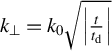 ${k}_{\perp }={k}_0\sqrt{\left|\frac{t}{t_\mathrm{d}}\right|}$
in the second case. Correspondingly, the condition of paraxial approximation
${k}_{\perp }={k}_0\sqrt{\left|\frac{t}{t_\mathrm{d}}\right|}$
in the second case. Correspondingly, the condition of paraxial approximation ${k}_{x,\perp}\ll {k}_0$
constrains the obtained results to the conditions
${k}_{x,\perp}\ll {k}_0$
constrains the obtained results to the conditions $\left|t\right|\ll 2\left|{\tau}_x\right|$
for
$\left|t\right|\ll 2\left|{\tau}_x\right|$
for ${\mathbb{C}}_\mathrm{s}(t)$
and
${\mathbb{C}}_\mathrm{s}(t)$
and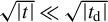 $\sqrt{\left|t\right|}\ll \sqrt{\left|{t}_\mathrm{d}\right|}$
for
$\sqrt{\left|t\right|}\ll \sqrt{\left|{t}_\mathrm{d}\right|}$
for ${\mathbb{C}}_\mathrm{d}(t)$
. Further investigation of
${\mathbb{C}}_\mathrm{d}(t)$
. Further investigation of $\mathbb{C}(t)$
, including quantitative comparison with
$\mathbb{C}(t)$
, including quantitative comparison with ${\mathbb{C}}_\mathrm{d}(t)$
and
${\mathbb{C}}_\mathrm{d}(t)$
and ${\mathbb{C}}_\mathrm{s}(t)$
, is possible only for the functional forms
${\mathbb{C}}_\mathrm{s}(t)$
, is possible only for the functional forms $\mathrm{PSD}{2}_{\Theta}, \mathrm{PSD}{2}_{\mathcal{A}}\kern0.36em \mathrm{and}\ \mathrm{PSD}{2}_{\varphi}$
.
$\mathrm{PSD}{2}_{\Theta}, \mathrm{PSD}{2}_{\mathcal{A}}\kern0.36em \mathrm{and}\ \mathrm{PSD}{2}_{\varphi}$
.
3 Power spectral density functional form PSD2 for obscurations on the grating/mirror surface
To find $\mathrm{PSD}{2}_{\Theta}\left({k}_{\perp}\right)$
for the field reflected from a surface with obscuration, we assume that the obscurations do not overlap each other and are shaped as a circle with coordinates of the centre
$\mathrm{PSD}{2}_{\Theta}\left({k}_{\perp}\right)$
for the field reflected from a surface with obscuration, we assume that the obscurations do not overlap each other and are shaped as a circle with coordinates of the centre ${\boldsymbol{R}}_{m}$
and radius
${\boldsymbol{R}}_{m}$
and radius ${w}_{m}$
:
${w}_{m}$
:
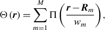 $$\begin{align}\Theta \left(\boldsymbol{r}\right)=\sum \limits_{m=1}^M\Pi \left(\frac{\boldsymbol{r}-{\boldsymbol{R}}_{m}}{w_{m}}\right),\end{align}$$
where $\Pi (x)=1\;\mathrm{if}\;\left|x\right|<1,\mathrm{otherwise}\;\Pi =0$
, and
$\Pi (x)=1\;\mathrm{if}\;\left|x\right|<1,\mathrm{otherwise}\;\Pi =0$
, and $M\gg 1$
is the number of obscurations. Here,
$M\gg 1$
is the number of obscurations. Here, ${\boldsymbol{R}}_m$
and
${\boldsymbol{R}}_m$
and ${w}_m$
are random quantities, with
${w}_m$
are random quantities, with ${\boldsymbol{R}}_m$
being uniformly distributed over the beam aperture and
${\boldsymbol{R}}_m$
being uniformly distributed over the beam aperture and ${w}_m$
having a probability density
${w}_m$
having a probability density $f(w)$
. It is obvious that
$f(w)$
. It is obvious that ${S}_\mathrm{ob}=\pi \sum_{m=1}^M{R}_{m}^2$
. The squared modulus of the noise spectrum
${S}_\mathrm{ob}=\pi \sum_{m=1}^M{R}_{m}^2$
. The squared modulus of the noise spectrum ${S}_{\Theta}$
is an incoherent sum of the squared moduli of the spectra
${S}_{\Theta}$
is an incoherent sum of the squared moduli of the spectra ${S}_m$
of flat-top beams having radius
${S}_m$
of flat-top beams having radius ${w}_m$
(Airy functions):
${w}_m$
(Airy functions):
 $$\begin{align}{S}_{\Theta}\left({k}_{\perp}\right)=\sum \limits_{m=1}^M{S}_{m}={I}_0\sum \limits_{m=1}^M{w}_{m}^4\frac{J_1^2\left({k}_{\perp }{w}_{m}\right)}{{\left({k}_{\perp }{w}_{m}\right)}^2},\end{align}$$
where ${J}_1$
is the Bessel function and
${J}_1$
is the Bessel function and ${I}_0={\left|{E}_0\right|}^2$
is the incident beam intensity assumed for simplicity to be equal for all obscurations. Here we sum the spectra incoherently, since the spectral phase of each obscuration is random and the sum of a large number of terms with random phase is zero. As a consequence,
${I}_0={\left|{E}_0\right|}^2$
is the incident beam intensity assumed for simplicity to be equal for all obscurations. Here we sum the spectra incoherently, since the spectral phase of each obscuration is random and the sum of a large number of terms with random phase is zero. As a consequence, ${S}_{\Theta}$
does not depend on
${S}_{\Theta}$
does not depend on ${\boldsymbol{R}}_{m}$
. From the definition of PSD2 in Equation (18) and of the Fourier spectrum in Equation (5), with allowance for ergodicity we obtain
${\boldsymbol{R}}_{m}$
. From the definition of PSD2 in Equation (18) and of the Fourier spectrum in Equation (5), with allowance for ergodicity we obtain $\mathrm{PSD}{2}_{\Theta}\left({k}_{\perp}\right)=\frac{<{S}_{\Theta}\left({k}_{\perp}\right)>}{I_0{S}_0}$
. By averaging Equation (31) we find the following:
$\mathrm{PSD}{2}_{\Theta}\left({k}_{\perp}\right)=\frac{<{S}_{\Theta}\left({k}_{\perp}\right)>}{I_0{S}_0}$
. By averaging Equation (31) we find the following:
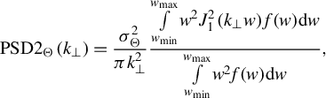 $$\begin{align}\mathrm{PSD}{2}_{\Theta}\left({k}_{\perp}\right)=\frac{\sigma_{\Theta}^2}{\pi {k}_{\perp}^2}\frac{\underset{{w}_\mathrm{min}}{\overset{{w}_\mathrm{max}}{\int }}{w}^2{J}_1^2\left({k}_{\perp }w\right)f(w) \mathrm{d}w}{\underset{w_\mathrm{min}}{\overset{w_\mathrm{max}}{\int }}{w}^2f(w) \mathrm{d}w},\end{align}$$
which, with Equation (27) taken into account, follows
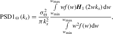 $$\begin{align}\mathrm{PSD}{1}_{\Theta}\left({k}_x\right)=\frac{\sigma_{\Theta}^2}{\pi {k}_x^2}\frac{\underset{{w}_\mathrm{min}}{\overset{{w}_\mathrm{max}}{\int }} wf(w){\boldsymbol{H}}_{1}\left(2w{k}_x\right) \mathrm{d}w}{\underset{w_\mathrm{min}}{\overset{w_\mathrm{max}}{\int }}{w}^2f(w) \mathrm{d}w},\end{align}$$
where ${\boldsymbol{H}}_{1}$
is the Struve function and
${\boldsymbol{H}}_{1}$
is the Struve function and ${w}_{\mathit{\min},\mathit{\max}}$
are the minimum and maximum radii of the obscurations. Obviously,
${w}_{\mathit{\min},\mathit{\max}}$
are the minimum and maximum radii of the obscurations. Obviously, $2{w}_\mathrm{min}\gg {\lambda}_0$
, since the paraxial approximation does not hold otherwise. Similarly, the obscurations with radius
$2{w}_\mathrm{min}\gg {\lambda}_0$
, since the paraxial approximation does not hold otherwise. Similarly, the obscurations with radius $w$
commensurate with the beam radius
$w$
commensurate with the beam radius ${R}_0$
cannot exist, since in this case the condition
${R}_0$
cannot exist, since in this case the condition ${W}_{\Theta}\ll {W}_0$
is violated. This imposes the constraint
${W}_{\Theta}\ll {W}_0$
is violated. This imposes the constraint ${w}_\mathrm{max}\ll {R}_0$
. In practice, the quantities
${w}_\mathrm{max}\ll {R}_0$
. In practice, the quantities ${w}_{\mathit{\min},\mathit{\max}}$
may have even more stringent constraints. Note that Equations (32) and (33) satisfy Equations (19) and (28) regardless of the form of the function
${w}_{\mathit{\min},\mathit{\max}}$
may have even more stringent constraints. Note that Equations (32) and (33) satisfy Equations (19) and (28) regardless of the form of the function $f(w)$
.
$f(w)$
. $\mathrm{PSD}{2}_{\Theta}$
is normalized to
$\mathrm{PSD}{2}_{\Theta}$
is normalized to $\frac{\sigma^2{w}_\mathrm{min}^4}{\pi <{w}^2>}$
as a function of
$\frac{\sigma^2{w}_\mathrm{min}^4}{\pi <{w}^2>}$
as a function of $\kappa ={k}_{\perp }{w}_\mathrm{min}$
for
$\kappa ={k}_{\perp }{w}_\mathrm{min}$
for $\xi =3.9$
(a) and
$\xi =3.9$
(a) and $\xi =3.1$
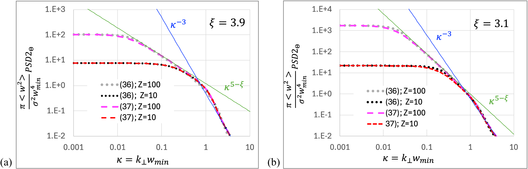
(b). Dotted curves represent exact Equation (36) values for Z = 100 (grey) and Z = 10 (black); dashed curves represent approximate Equation (37) values for Z = 100 (pink) and Z = 10 (red).
$\xi =3.1$
(b). Dotted curves represent exact Equation (36) values for Z = 100 (grey) and Z = 10 (black); dashed curves represent approximate Equation (37) values for Z = 100 (pink) and Z = 10 (red).
Next, it is necessary to substitute into Equations (32) and (33) $f(w)$
of a specific form, which may be quite complex. For example, for the optics of the standard indicated in Ref. [48],
$f(w)$
of a specific form, which may be quite complex. For example, for the optics of the standard indicated in Ref. [48], $f(w)$
has the form
$f(w)$
has the form $\log f(w)\sim {(\log w)}^2$
. We will restrict our consideration to the power form:
$\log f(w)\sim {(\log w)}^2$
. We will restrict our consideration to the power form:
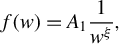 $$\begin{align}f(w)={A}_1\frac{1}{w^{\xi }},\end{align}$$
given in Ref. [Reference Spaeth, Manes, Widmayer, Williams, Whitman, Henesian, Stowers and Honig23] for surface defects of optical elements after their use in a high-power laser facility. Under the almost always met condition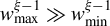 ${w}_\mathrm{max}^{\xi -1}\gg {w}_\mathrm{min}^{\xi -1}$
, from
${w}_\mathrm{max}^{\xi -1}\gg {w}_\mathrm{min}^{\xi -1}$
, from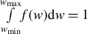 $\underset{w_\mathrm{min}}{\overset{w_\mathrm{max}}{\int }}f(w) \mathrm{d}w=1$
we obtain
$\underset{w_\mathrm{min}}{\overset{w_\mathrm{max}}{\int }}f(w) \mathrm{d}w=1$
we obtain ${A}_1=\left(\xi -1\right){w}_\mathrm{min}^{\xi -1}$
, that is,
${A}_1=\left(\xi -1\right){w}_\mathrm{min}^{\xi -1}$
, that is, $f(w)$
does not depend on
$f(w)$
does not depend on ${w}_\mathrm{max}$
. The data reported in Ref. [Reference Spaeth, Manes, Widmayer, Williams, Whitman, Henesian, Stowers and Honig23] correspond to
${w}_\mathrm{max}$
. The data reported in Ref. [Reference Spaeth, Manes, Widmayer, Williams, Whitman, Henesian, Stowers and Honig23] correspond to $\xi =3.9$
and
$\xi =3.9$
and ${w}_\mathrm{min}\approx 0.025\;\mathrm{mm}$
. Before using the optical elements in the high-power laser facility, the distribution function
${w}_\mathrm{min}\approx 0.025\;\mathrm{mm}$
. Before using the optical elements in the high-power laser facility, the distribution function $f(w)$
is also defined by Equation (34) with
$f(w)$
is also defined by Equation (34) with $\xi =3.9$
, but the laser damage was 7.8 times less[
Reference Spaeth, Manes, Widmayer, Williams, Whitman, Henesian, Stowers and Honig
23
,
Reference Stowers, Horvath, Menapace, Burnham and Letts
49
]. In what follows, we will assume
$\xi =3.9$
, but the laser damage was 7.8 times less[
Reference Spaeth, Manes, Widmayer, Williams, Whitman, Henesian, Stowers and Honig
23
,
Reference Stowers, Horvath, Menapace, Burnham and Letts
49
]. In what follows, we will assume $\xi$
and
$\xi$
and ${w}_\mathrm{min}$
to be arbitrary constants and use the above values only for constructing specific plots in Section 6. The moments
${w}_\mathrm{min}$
to be arbitrary constants and use the above values only for constructing specific plots in Section 6. The moments $<{w}^n>$
are readily calculated from Equation (34):
$<{w}^n>$
are readily calculated from Equation (34):
 $$\begin{align}<{w}^n>=\underset{w_\mathrm{min}}{\overset{w_\mathrm{max}}{\int }}{w}^nf(w) \mathrm{d}w={w}_\mathrm{min}^n\frac{\xi -1}{\xi -n-1}\left(1-{Z}^{n-\xi +1}\right),\end{align}$$
where $Z={w}_\mathrm{max}/{w}_\mathrm{min}$
. For
$Z={w}_\mathrm{max}/{w}_\mathrm{min}$
. For $\xi =n+1$
, Equation (35) is valid within the limit
$\xi =n+1$
, Equation (35) is valid within the limit $\xi \to n+1$
. On substituting Equation (34) into Equations (32) and (33) and passing to dimensionless quantities
$\xi \to n+1$
. On substituting Equation (34) into Equations (32) and (33) and passing to dimensionless quantities $\kappa ={k}_{\perp }{w}_\mathrm{min}$
and
$\kappa ={k}_{\perp }{w}_\mathrm{min}$
and $K={k}_x{w}_\mathrm{min}$
, we obtain the following:
$K={k}_x{w}_\mathrm{min}$
, we obtain the following:
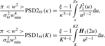 $$\begin{align}\frac{\pi <{w}^2>}{\sigma_{\Theta}^2{w}_\mathrm{min}^4} \mathrm{PSD}{2}_{\Theta}\left(\kappa \right)&=\frac{\xi -1}{\kappa^{5-\xi }}\underset{\kappa }{\overset{Z\kappa}{\int }}\frac{J_1^2(u)}{u^{\xi -2}} \mathrm{d}u,\nonumber\\\frac{\pi <{w}^2>}{\sigma_{\Theta}^2{w}_\mathrm{min}^3} \mathrm{PSD}{1}_{\Theta}(K)&=\frac{\xi -1}{K^{4-\xi }}\underset{K}{\overset{KZ}{\int }}\frac{{\boldsymbol{H}}_{1}(2u)}{u^{\xi -1}} \mathrm{d}u.\end{align}$$
Both integrals in Equation (36) are expressed only through the generalized hypergeometric function $_2{F}_3$
, which complicates further analytical analysis. The expression in Equation (36) can be significantly simplified in three special cases: for
$_2{F}_3$
, which complicates further analytical analysis. The expression in Equation (36) can be significantly simplified in three special cases: for ${k}_{\perp }{w}_\mathrm{max}\ll 1$
and
${k}_{\perp }{w}_\mathrm{max}\ll 1$
and ${k}_{\perp }{w}_\mathrm{min}\gg 1$
, the functions
${k}_{\perp }{w}_\mathrm{min}\gg 1$
, the functions ${J}_1$
and
${J}_1$
and ${\boldsymbol{H}}_{1}$
may be replaced by their asymptotic forms, and for
${\boldsymbol{H}}_{1}$
may be replaced by their asymptotic forms, and for ${w}_\mathrm{max}^{-1}\ll {k}_{\perp, x}\ll {w}_\mathrm{min}^{-1}$
, the integration limits may be replaced by 0 and
${w}_\mathrm{max}^{-1}\ll {k}_{\perp, x}\ll {w}_\mathrm{min}^{-1}$
, the integration limits may be replaced by 0 and $\infty$
. In all special cases, a power-law dependence is obtained: in three sections of the spectrum
$\infty$
. In all special cases, a power-law dependence is obtained: in three sections of the spectrum ${k}_{\perp, x}{w}_\mathrm{max}\ll 1$
,
${k}_{\perp, x}{w}_\mathrm{max}\ll 1$
, ${w}_\mathrm{max}^{-1}\ll {k}_{\perp, x}\ll {w}_\mathrm{min}^{-1}$
and
${w}_\mathrm{max}^{-1}\ll {k}_{\perp, x}\ll {w}_\mathrm{min}^{-1}$
and ${k}_{\perp, x}{w}_\mathrm{min}\gg 1,$ $\mathrm{PSD}{2}_{\Theta}$
decreases in a power-law manner with powers
$\mathrm{PSD}{2}_{\Theta}$
decreases in a power-law manner with powers $0,5-\xi\;\mathrm{and}\;3$
, and
$0,5-\xi\;\mathrm{and}\;3$
, and $\mathrm{PSD}{1}_{\Theta}$
with powers
$\mathrm{PSD}{1}_{\Theta}$
with powers $0,4-\xi\;\mathrm{and}\;2$
. This is demonstrated in Figure 3 where
$0,4-\xi\;\mathrm{and}\;2$
. This is demonstrated in Figure 3 where $\mathrm{PSD}{2}_{\Theta}\left({k}_{\perp}\right)$
in Equation (36) is plotted. The
$\mathrm{PSD}{2}_{\Theta}\left({k}_{\perp}\right)$
in Equation (36) is plotted. The $\mathrm{PSD}1\left({k}_x\right)$
curves look similar. From Figure 3 it can be seen that
$\mathrm{PSD}1\left({k}_x\right)$
curves look similar. From Figure 3 it can be seen that $\mathrm{PSD}{2}_{\Theta}\left({k}_{\perp}\right)$
is well approximated by the following expression:
$\mathrm{PSD}{2}_{\Theta}\left({k}_{\perp}\right)$
is well approximated by the following expression:
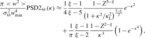 $$\begin{align}\frac{\pi <{w}^2>}{\sigma_{\Theta}^2{w}_\mathrm{min}^4} \mathrm{PSD}{2}_{\Theta}\left(\kappa \right)&\approx \frac{1}{4}\frac{\xi -1}{\xi -5}\frac{1-{Z}^{5-\xi }}{{\left(1+{\kappa}^2/{\kappa}_\mathrm{L}^2\right)}^{\frac{5-\xi }{2}}}{e}^{-{\kappa}^2}\nonumber\\&\quad+\frac{1}{\pi}\frac{\xi -1}{\xi -2}\frac{1-{Z}^{2-\xi }}{\kappa^3}\left(1-{e}^{-{\kappa}^4}\right),\end{align}$$
where
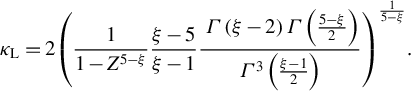 $$\begin{align}{\kappa}_\mathrm{L}=2{\left(\frac{1}{1-{Z}^{5-\xi }}\frac{\xi -5}{\xi -1}\frac{\;\varGamma \left(\xi -2\right)\varGamma \left(\frac{5-\xi }{2}\right)}{\varGamma^3\left(\frac{\xi -1}{2}\right)}\right)}^{\frac{1}{5-\xi }}.\end{align}$$
Compare the black and grey dotted curves with the red and pink dashed curves in the figure. If ${Z}^{5-\xi}\gg 1$
, which is true for
${Z}^{5-\xi}\gg 1$
, which is true for $\xi =3.9$
, then
$\xi =3.9$
, then ${\kappa}_\mathrm{L}$
is proportional to
${\kappa}_\mathrm{L}$
is proportional to ${Z}^{-1}$
, that is, to
${Z}^{-1}$
, that is, to ${w}_\mathrm{max}^{-1}$
(see Equation (38)). At the frequencies
${w}_\mathrm{max}^{-1}$
(see Equation (38)). At the frequencies ${k}_{\perp}\gg {w}_\mathrm{max}^{-1}$
, the product
${k}_{\perp}\gg {w}_\mathrm{max}^{-1}$
, the product $\left(<{w}^2> \mathrm{PSD}{2}_{\Theta}\right)$
does not depend on Z – the grey and black dotted curves in Figure 3 coincide. Since the low frequencies
$\left(<{w}^2> \mathrm{PSD}{2}_{\Theta}\right)$
does not depend on Z – the grey and black dotted curves in Figure 3 coincide. Since the low frequencies ${k}_{\perp}\leq {w}_\mathrm{max}^{-1}$
contribute only to contrast at small times (see Section 2),
${k}_{\perp}\leq {w}_\mathrm{max}^{-1}$
contribute only to contrast at small times (see Section 2), $Z$
affects the contrast only slightly.
$Z$
affects the contrast only slightly.
4 Power spectral density functional form
$\mathbf{PSD}_{\mathbf{r}}$
for roughness of the grating/mirror surface

The surface profile $h\left(\boldsymbol{r}\right)$
is characterized by the function
$h\left(\boldsymbol{r}\right)$
is characterized by the function $\mathrm{PSD}{2}_\mathrm{h}\left({k}_{\perp}\right)$
related to the PSD of the introduced phase fluctuations
$\mathrm{PSD}{2}_\mathrm{h}\left({k}_{\perp}\right)$
related to the PSD of the introduced phase fluctuations $\mathrm{PSD}{2}_\mathrm{r}\left({k}_{\perp}\right)$
by the following:
$\mathrm{PSD}{2}_\mathrm{r}\left({k}_{\perp}\right)$
by the following:
 $$\begin{align}\mathrm{PSD}{2}_\mathrm{r}\left({k}_{\perp}\right)={B}_0{k}_0^2 \mathrm{PSD}{2}_\mathrm{h}\left({k}_{\perp}\right),\end{align}$$
where ${B}_0={\left( \cos\alpha + \cos\beta \right)}^2$
for the grating[
Reference Khazanov
50
] and
${B}_0={\left( \cos\alpha + \cos\beta \right)}^2$
for the grating[
Reference Khazanov
50
] and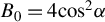 ${B}_0=4{\mathit{\cos}}^2\alpha$
for the mirror. Much attention in the literature has been paid to measuring
${B}_0=4{\mathit{\cos}}^2\alpha$
for the mirror. Much attention in the literature has been paid to measuring $\mathrm{PSD}{1}_\mathrm{h}\left({k}_x\right)$
[
Reference Webb, Dorrer, Bahk, Jeon, Roides and Bromage
5
,
Reference Roeder, Zobus, Major and Bagnoud
11
,
Reference Ranc, Blanc, Lebas, Martin, Zou, Mathieu, Radier, Ricaud, Druon and Papadopoulos
14
,
Reference Roeder, Zobus, Brabetz and Bagnoud
19
,
Reference Spaeth, Manes, Widmayer, Williams, Whitman, Henesian, Stowers and Honig
23
,
Reference Khazanov, Kochetkov and Silin
45
,
Reference Church
51
–
Reference Camus, Coic, Blanchot, Bouillet, Lavastre, Mangeant, Rouyer and Néauport
55
]. In general, it behaves differently in different spectral ranges for different optical elements. In such a case, it is necessary to substitute the experimental data into Equations (39) and (27) and the result into Equation (25). At medium and high spatial frequencies,
$\mathrm{PSD}{1}_\mathrm{h}\left({k}_x\right)$
[
Reference Webb, Dorrer, Bahk, Jeon, Roides and Bromage
5
,
Reference Roeder, Zobus, Major and Bagnoud
11
,
Reference Ranc, Blanc, Lebas, Martin, Zou, Mathieu, Radier, Ricaud, Druon and Papadopoulos
14
,
Reference Roeder, Zobus, Brabetz and Bagnoud
19
,
Reference Spaeth, Manes, Widmayer, Williams, Whitman, Henesian, Stowers and Honig
23
,
Reference Khazanov, Kochetkov and Silin
45
,
Reference Church
51
–
Reference Camus, Coic, Blanchot, Bouillet, Lavastre, Mangeant, Rouyer and Néauport
55
]. In general, it behaves differently in different spectral ranges for different optical elements. In such a case, it is necessary to substitute the experimental data into Equations (39) and (27) and the result into Equation (25). At medium and high spatial frequencies, $\mathrm{PSD}{2}_\mathrm{h}$
often has a power-law form, and at low frequencies it is equal to a constant. Therefore,
$\mathrm{PSD}{2}_\mathrm{h}$
often has a power-law form, and at low frequencies it is equal to a constant. Therefore, $\mathrm{PSD}{2}_\mathrm{h}$
is well approximated by a Lorentz-type spectrum[
Reference Bromage, Dorrer and Jungquist
21
,
Reference Khazanov, Kochetkov and Silin
45
,
Reference Harvey, Schröder, Choi and Duparré
56
] with correlation length
$\mathrm{PSD}{2}_\mathrm{h}$
is well approximated by a Lorentz-type spectrum[
Reference Bromage, Dorrer and Jungquist
21
,
Reference Khazanov, Kochetkov and Silin
45
,
Reference Harvey, Schröder, Choi and Duparré
56
] with correlation length $1/{k}_\mathrm{h}$
, surface profile dispersion
$1/{k}_\mathrm{h}$
, surface profile dispersion ${\sigma}_\mathrm{h}^2$
and exponent
${\sigma}_\mathrm{h}^2$
and exponent $a>2$
. Then
$a>2$
. Then
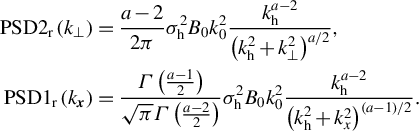 $$\begin{align}\mathrm{PSD}{2}_\mathrm{r}\left({k}_{\perp}\right)&=\frac{a-2}{2\pi }{\sigma}_\mathrm{h}^2{B}_0{k}_0^2\frac{k_\mathrm{h}^{a-2}}{{\left({k}_\mathrm{h}^2+{k}_{\perp}^2\right)}^{a/2}},\kern0.72em\nonumber\\\mathrm{PSD}{1}_\mathrm{r}\left({k}_{\boldsymbol{x}}\right)&=\frac{\varGamma \left(\frac{a-1}{2}\right)}{\sqrt{\pi}\varGamma \left(\frac{a-2}{2}\right)}{\sigma}_\mathrm{h}^2{B}_0{k}_0^2\frac{k_\mathrm{h}^{a-2}}{{\left({k}_\mathrm{h}^2+{k}_x^2\right)}^{\left(a-1\right)/2}}.\end{align}$$
Usually, $2<a<4$
. A frequently encountered value is
$2<a<4$
. A frequently encountered value is $a\approx 2.55$
, including in Ref. [Reference Hu, Wan, Jiang, Gu, Zhang, Jin, Liu, Zhao, Cao, Wei and Shao54], where
$a\approx 2.55$
, including in Ref. [Reference Hu, Wan, Jiang, Gu, Zhang, Jin, Liu, Zhao, Cao, Wei and Shao54], where $\mathrm{PSD}{1}_\mathrm{h}\left({k}_{\perp}\right)$
was measured for an off-axis parabola used for writing holographic gratings.
$\mathrm{PSD}{1}_\mathrm{h}\left({k}_{\perp}\right)$
was measured for an off-axis parabola used for writing holographic gratings.
5 Power spectral density functional form for obscuration and roughness of the optics used for writing gratings
When writing a holographic grating, even with a perfectly plane substrate surface, the grating is not ideal due to the non-equidistance and non-parallelism of the grooves, as well as due to groove profile fluctuations.
The non-equidistance and non-parallelism of the grooves are determined by spatial fluctuations in the phase difference of two writing beams and give rise to fluctuations in the phase of the beam reflected from the grating $\Delta \varphi \left(\boldsymbol{r}\right)\ne 0$
[
Reference Bienert, Röcker, Dietrich, Graf and Ahmed
25
–
Reference Kochetkov, Shaykin, Yakovlev, Khazanov, Cheplakov, Wang, Jin, Liu and Shao
28
], without affecting the reflection coefficient:
$\Delta \varphi \left(\boldsymbol{r}\right)\ne 0$
[
Reference Bienert, Röcker, Dietrich, Graf and Ahmed
25
–
Reference Kochetkov, Shaykin, Yakovlev, Khazanov, Cheplakov, Wang, Jin, Liu and Shao
28
], without affecting the reflection coefficient: $\mathcal{A}\left(\boldsymbol{r}\right)=~0$
. For a holographic grating this phase is equal to the phase of the writing field
$\mathcal{A}\left(\boldsymbol{r}\right)=~0$
. For a holographic grating this phase is equal to the phase of the writing field ${\phi}_\mathrm{wr}$
scaled along the x-axis[
Reference Khazanov
27
]:
${\phi}_\mathrm{wr}$
scaled along the x-axis[
Reference Khazanov
27
]: $\Delta \varphi \left(\boldsymbol{r}\right)={\phi}_\mathrm{wr}\left( x\cos\Phi, y\right)$
. Here,
$\Phi$
is the angle of incidence on the substrate (Figure 4) and
$\Delta \varphi \left(\boldsymbol{r}\right)={\phi}_\mathrm{wr}\left( x\cos\Phi, y\right)$
. Here,
$\Phi$
is the angle of incidence on the substrate (Figure 4) and $\sin\Phi =N{\lambda}_\mathrm{wr}/2$
. The phase
$\sin\Phi =N{\lambda}_\mathrm{wr}/2$
. The phase $\Delta \varphi \left(\boldsymbol{r}\right)$
is added to the phase
$\Delta \varphi \left(\boldsymbol{r}\right)$
is added to the phase $\varphi \left(\boldsymbol{r}\right)$
associated with the non-flat surface of the grating that was discussed in Section 4. Since these phases are uncorrelated, their PSDs are summed. Considering that
$\varphi \left(\boldsymbol{r}\right)$
associated with the non-flat surface of the grating that was discussed in Section 4. Since these phases are uncorrelated, their PSDs are summed. Considering that $\cos\Phi$
is usually close to unity, we will assume that the PSD functions for
$\cos\Phi$
is usually close to unity, we will assume that the PSD functions for $\Delta \varphi$
and
$\Delta \varphi$
and ${\phi}_\mathrm{wr}$
are equal and designate them as
${\phi}_\mathrm{wr}$
are equal and designate them as $\mathrm{PSD}{2}_\mathrm{phase}$
.
$\mathrm{PSD}{2}_\mathrm{phase}$
.
Scheme of writing holographic diffraction grating by two laser beams. BS, beamsplitter; M1–M5, mirrors; SF, spatial filters.
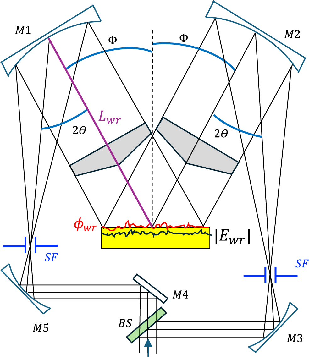
The fluctuations in the groove shape are caused by spatial fluctuations in the intensity of the radiation used to write the grating and give rise to the fluctuations in the modulus of the grating reflectivity $\mathcal{A}\left(\boldsymbol{r}\right)\ne 0$
[
Reference Koch, Lehr and Glaser
24
], without affecting its phase:
$\mathcal{A}\left(\boldsymbol{r}\right)\ne 0$
[
Reference Koch, Lehr and Glaser
24
], without affecting its phase: $\Delta \varphi \left(\boldsymbol{r}\right)=0$
. Rigorous calculation of the PSD of the grating reflectivity fluctuations
$\Delta \varphi \left(\boldsymbol{r}\right)=0$
. Rigorous calculation of the PSD of the grating reflectivity fluctuations $\mathrm{PSD}{2}_{\mathcal{A}}$
is a complex problem that requires knowledge of the exact relationship between these fluctuations and the intensity fluctuations of the writing field
$\mathrm{PSD}{2}_{\mathcal{A}}$
is a complex problem that requires knowledge of the exact relationship between these fluctuations and the intensity fluctuations of the writing field ${\left|{E}_\mathrm{wr}\left(\boldsymbol{r}\right)\right|}^2$
. However, taking into account the smallness of both fluctuations relative to their mean values, we will assume that they are proportional to each other. Then
${\left|{E}_\mathrm{wr}\left(\boldsymbol{r}\right)\right|}^2$
. However, taking into account the smallness of both fluctuations relative to their mean values, we will assume that they are proportional to each other. Then $\mathrm{PSD}{2}_{\mathcal{A}}= q\mathrm{PSD}{2}_\mathrm{dose}$
, where
$\mathrm{PSD}{2}_{\mathcal{A}}= q\mathrm{PSD}{2}_\mathrm{dose}$
, where $q>0$
is a dimensionless coefficient and
$q>0$
is a dimensionless coefficient and $\mathrm{PSD}{2}_\mathrm{dose}$
is
$\mathrm{PSD}{2}_\mathrm{dose}$
is $\mathrm{PSD}2$
for the radiation intensity on the substrate normalized to the average value. Now we need to find
$\mathrm{PSD}2$
for the radiation intensity on the substrate normalized to the average value. Now we need to find $\mathrm{PSD}{2}_\mathrm{phase}$
and
$\mathrm{PSD}{2}_\mathrm{phase}$
and $\mathrm{PSD}{2}_\mathrm{dose}$
.
$\mathrm{PSD}{2}_\mathrm{dose}$
.
Since all dynamic noises are averaged during grating exposure, only the ‘frozen’ noises caused by the imperfection of the transport optics are significant. Obviously, the fewer optical elements are used, the better. A scheme for writing a holographic grating that is optimal from this point of view is presented in Figure 4
[
Reference Hu, Wan, Jiang, Gu, Zhang, Jin, Liu, Zhao, Cao, Wei and Shao
54
]. Since the spatial filter ensures good filtering of high-frequency noise, only the transport optics located after the filters are of fundamental importance. The scheme in Figure 4 contains a minimum number of such elements – two off-axis parabolic mirrors (OAPs). In the classical work[
Reference Boyd, Britten, Decker, Shore, Stuart, Perry and Li
57
] and other[
Reference Koch, Lehr and Glaser
24
] papers, collimators are additionally used, which increases fluctuations. When reflecting the beam ${E}_\mathrm{wr}\left(\boldsymbol{r}\right)$
these two OAPs introduce into it both amplitude noise caused by scratches and defects (obscuration) and phase noise caused by the imperfection/roughness of the surface. Let us denote by
${E}_\mathrm{wr}\left(\boldsymbol{r}\right)$
these two OAPs introduce into it both amplitude noise caused by scratches and defects (obscuration) and phase noise caused by the imperfection/roughness of the surface. Let us denote by $\mathrm{PSD}{2}_{\mathrm{m},\Theta}$
and
$\mathrm{PSD}{2}_{\mathrm{m},\Theta}$
and $\mathrm{PSD}{2}_{\mathrm{m},\varphi }$
the PSD of the amplitude and phase of the field reflected from the OAP. We assume that the statistical properties of the OAP surface are the same as the properties of the grating surface, that is, they have equal
$\mathrm{PSD}{2}_{\mathrm{m},\varphi }$
the PSD of the amplitude and phase of the field reflected from the OAP. We assume that the statistical properties of the OAP surface are the same as the properties of the grating surface, that is, they have equal $\mathrm{PSD}{2}_\mathrm{h}\left({k}_{\perp}\right)$
. Then
$\mathrm{PSD}{2}_\mathrm{h}\left({k}_{\perp}\right)$
. Then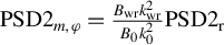 $\mathrm{PSD}{2}_{m,\varphi }=\frac{B_\mathrm{wr}{k}_\mathrm{wr}^2}{B_0{k}_0^2} \mathrm{PSD}{2}_\mathrm{r}$
, Equation (40), where
$\mathrm{PSD}{2}_{m,\varphi }=\frac{B_\mathrm{wr}{k}_\mathrm{wr}^2}{B_0{k}_0^2} \mathrm{PSD}{2}_\mathrm{r}$
, Equation (40), where ${k}_\mathrm{wr}$
is the wave vector of the writing radiation and
${k}_\mathrm{wr}$
is the wave vector of the writing radiation and ${B}_\mathrm{wr}=4{\mathit{\cos}}^2\theta$
, where
${B}_\mathrm{wr}=4{\mathit{\cos}}^2\theta$
, where $\theta$
is the angle of incidence on the OAP (Figure 4). Analogously, we assume that the statistical properties of obscuration on these mirrors are the same as on the gratings, that is,
$\theta$
is the angle of incidence on the OAP (Figure 4). Analogously, we assume that the statistical properties of obscuration on these mirrors are the same as on the gratings, that is,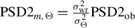 $\mathrm{PSD}{2}_{m,\Theta}=\frac{\sigma_\mathrm{wr}^2}{\sigma_{\Theta}^2} \mathrm{PSD}{2}_\mathrm{ob}$
, Equation (37). For unused gratings it is reasonable to assume that
$\mathrm{PSD}{2}_{m,\Theta}=\frac{\sigma_\mathrm{wr}^2}{\sigma_{\Theta}^2} \mathrm{PSD}{2}_\mathrm{ob}$
, Equation (37). For unused gratings it is reasonable to assume that ${\sigma}_{\Theta}^2={\sigma}_\mathrm{wr}^2$
, but with long-term use of gratings in high-power radiation the number of defects increases and
${\sigma}_{\Theta}^2={\sigma}_\mathrm{wr}^2$
, but with long-term use of gratings in high-power radiation the number of defects increases and ${\sigma}_{\Theta}^2\gg {\sigma}_\mathrm{wr}^2$
; see Section 3.
${\sigma}_{\Theta}^2\gg {\sigma}_\mathrm{wr}^2$
; see Section 3.
The field on the substrate differs from the field on the mirror, since when the light is propagating from the mirror to the substrate over distance ${L}_\mathrm{wr}$
, the fluctuations of the amplitude and phase of the field transform into each other. An expression for
${L}_\mathrm{wr}$
, the fluctuations of the amplitude and phase of the field transform into each other. An expression for $\mathrm{PSD}{2}_\mathrm{dose}$
when a beam propagates in free space was obtained in Ref. [Reference Martyanov and Khazanov44], from which, in the particular case of monochromatic radiation of interests to us, we find the following:
$\mathrm{PSD}{2}_\mathrm{dose}$
when a beam propagates in free space was obtained in Ref. [Reference Martyanov and Khazanov44], from which, in the particular case of monochromatic radiation of interests to us, we find the following:
 $$\begin{align}&\mathrm{PSD}{2}_\mathrm{dose}=4T\left( \mathrm{PSD}{2}_{\mathrm{m},\Theta}+ \mathrm{PSD}{2}_{\mathrm{m},\varphi}\right)\nonumber\\&\quad+4\mathit{\operatorname{Re}}\left({T}_2{e}^{i{L}_\mathrm{wr}{k}_{\perp}^2/{k}_0}\right)\left( \mathrm{PSD}{2}_{\mathrm{m},\Theta}- \mathrm{PSD}{2}_{\mathrm{m},\varphi}\right),\end{align}$$
where
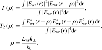 $$\begin{align}T\left(\boldsymbol{\rho} \right)&=\frac{\int {\left|{E}_\mathrm{wr}\left(\boldsymbol{r}\right)\right|}^2{\left|{E}_\mathrm{wr}\left(\boldsymbol{r}-\boldsymbol{\rho} \right)\right|}^2\mathrm{d}\boldsymbol{r}}{\int {\left|{E}_\mathrm{wr}\left(\boldsymbol{r}\right)\right|}^4\mathrm{d}\boldsymbol{r}},\kern0.72em\nonumber\\{T}_2\left(\boldsymbol{\rho} \right)&=\frac{\int {E}_\mathrm{wr}^{\ast}\left(\boldsymbol{r}-\boldsymbol{\rho} \right){E}_\mathrm{wr}^{\ast}\left(\boldsymbol{r}+\boldsymbol{\rho} \right){E}_\mathrm{wr}^2\left(\boldsymbol{r}\right)\mathrm{d}\boldsymbol{r}}{\int {\left|{E}_\mathrm{wr}\left(\boldsymbol{r}\right)\right|}^4\mathrm{d}\boldsymbol{r}},\kern0.72em\nonumber\\\boldsymbol{\rho} &=\frac{L_\mathrm{wr}{\boldsymbol{k}}_{\boldsymbol{\perp}}}{k_0}.\end{align}$$
Here, we took into account that two OAPs with uncorrelated noises contribute to $\mathrm{PSD}{2}_\mathrm{dose}$
, that is, the
$\mathrm{PSD}{2}_\mathrm{dose}$
, that is, the $\mathrm{PSD}{2}_\mathrm{dose}$
in Equation (41) is twice as large as that for one beam reported in Ref. [Reference Martyanov and Khazanov44]. It can be readily shown that the
$\mathrm{PSD}{2}_\mathrm{dose}$
in Equation (41) is twice as large as that for one beam reported in Ref. [Reference Martyanov and Khazanov44]. It can be readily shown that the $\mathrm{PSD}$
of field amplitude fluctuations
$\mathrm{PSD}$
of field amplitude fluctuations $\left|{E}_\mathrm{wr}\left(\boldsymbol{r}\right)\right|$
is four times smaller than the
$\left|{E}_\mathrm{wr}\left(\boldsymbol{r}\right)\right|$
is four times smaller than the $\mathrm{PSD}{2}_\mathrm{dose}$
, and the sum of the
$\mathrm{PSD}{2}_\mathrm{dose}$
, and the sum of the $\mathrm{PSD}$
of the field amplitude fluctuations
$\mathrm{PSD}$
of the field amplitude fluctuations $\left|{E}_\mathrm{wr}\left(\boldsymbol{r}\right)\right|$
and the
$\left|{E}_\mathrm{wr}\left(\boldsymbol{r}\right)\right|$
and the $\mathrm{PSD}$
of the field phase
$\mathrm{PSD}$
of the field phase ${\phi}_\mathrm{wr}\left(\boldsymbol{r}\right)$
is
${\phi}_\mathrm{wr}\left(\boldsymbol{r}\right)$
is $4T\left( \mathrm{PSD}{2}_{\mathrm{m},\Theta}+ \mathrm{PSD}{2}_{\mathrm{m},r}\right)$
. Thus,
$4T\left( \mathrm{PSD}{2}_{\mathrm{m},\Theta}+ \mathrm{PSD}{2}_{\mathrm{m},r}\right)$
. Thus, $\mathrm{PSD}{2}_\mathrm{phase}=\frac{1}{4} \mathrm{PSD}{2}_\mathrm{dose}$
.
$\mathrm{PSD}{2}_\mathrm{phase}=\frac{1}{4} \mathrm{PSD}{2}_\mathrm{dose}$
.
The authors of Ref. [Reference Hu, Wan, Jiang, Gu, Zhang, Jin, Liu, Zhao, Cao, Wei and Shao54] derived an expression similar to Equation (41) with $T=1$
, that is, neglecting the finite beam aperture
$T=1$
, that is, neglecting the finite beam aperture ${E}_\mathrm{wr}\left(\boldsymbol{r}\right)$
(see below). The term with
${E}_\mathrm{wr}\left(\boldsymbol{r}\right)$
(see below). The term with ${T}_2$
corresponds to the Talbot effect. Considering that
${T}_2$
corresponds to the Talbot effect. Considering that ${L}_\mathrm{wr}$
is of the order of 10 m, at large
${L}_\mathrm{wr}$
is of the order of 10 m, at large ${k}_{\perp }$
this term rapidly oscillates around zero. In addition, since the contribution to
${k}_{\perp }$
this term rapidly oscillates around zero. In addition, since the contribution to $\mathrm{PSD}{2}_{\mathrm{phase, dose}}$
is made by two surfaces with close but not identical distances
$\mathrm{PSD}{2}_{\mathrm{phase, dose}}$
is made by two surfaces with close but not identical distances ${L}_\mathrm{wr}$
, the total phase fluctuations at large
${L}_\mathrm{wr}$
, the total phase fluctuations at large ${k}_{\perp }$
are averaged. Therefore, this term can be approximately replaced by its average value, which is obviously equal to zero, that is, we can set
${k}_{\perp }$
are averaged. Therefore, this term can be approximately replaced by its average value, which is obviously equal to zero, that is, we can set ${T}_2=0$
. The function
${T}_2=0$
. The function $T\left(\boldsymbol{\rho} \right)$
corresponds to the spatial self-filtering of noise during propagation in free space[
Reference Martyanov and Khazanov
44
,
Reference Mironov, Lozhkarev, Luchinin, Shaykin and Khazanov
58
,
Reference Khazanov, Mironov and Mourou
59
], which is associated with the fact that part of the high-frequency noise escapes from the beam aperture. The transmittance
$T\left(\boldsymbol{\rho} \right)$
corresponds to the spatial self-filtering of noise during propagation in free space[
Reference Martyanov and Khazanov
44
,
Reference Mironov, Lozhkarev, Luchinin, Shaykin and Khazanov
58
,
Reference Khazanov, Mironov and Mourou
59
], which is associated with the fact that part of the high-frequency noise escapes from the beam aperture. The transmittance $T\left(\boldsymbol{\rho} \right),$
that is, the normalized autocorrelation function of the writing beam intensity, is close to unity at
$T\left(\boldsymbol{\rho} \right),$
that is, the normalized autocorrelation function of the writing beam intensity, is close to unity at $\rho \ll {R}_0$
, that is, for
$\rho \ll {R}_0$
, that is, for $\frac{L_\mathrm{wr}}{R_0}\ll \frac{k_0}{k_{\perp }}$
. Since
$\frac{L_\mathrm{wr}}{R_0}\ll \frac{k_0}{k_{\perp }}$
. Since ${L}_\mathrm{wr}\approx 10{R}_0$
, then
${L}_\mathrm{wr}\approx 10{R}_0$
, then $T\left(\boldsymbol{\rho} \right)\approx 1$
for
$T\left(\boldsymbol{\rho} \right)\approx 1$
for ${k}_{\perp}\ll 0.1{k}_0$
. This condition is more rigorous than the paraxial approximation condition
${k}_{\perp}\ll 0.1{k}_0$
. This condition is more rigorous than the paraxial approximation condition ${k}_{\perp}\ll {k}_0$
, so self-filtering cannot be completely neglected. At the same time,
${k}_{\perp}\ll {k}_0$
, so self-filtering cannot be completely neglected. At the same time, $T\left(\rho ={R}_0\right)\approx 1/2$
, that is, for
$T\left(\rho ={R}_0\right)\approx 1/2$
, that is, for ${k}_{\perp }=0.1{k}_0$
(the paraxial approximation boundary), the error will be about two. Therefore, assuming
${k}_{\perp }=0.1{k}_0$
(the paraxial approximation boundary), the error will be about two. Therefore, assuming $T\left(\boldsymbol{\rho} \right)\approx 1$
we obtain a slightly overestimated noise value at high (
$T\left(\boldsymbol{\rho} \right)\approx 1$
we obtain a slightly overestimated noise value at high ( ${k}_{\perp}\approx 0.1{k}_0$
) frequencies and, consequently, a slightly overestimated contrast value at large times. From Equation (41), with
${k}_{\perp}\approx 0.1{k}_0$
) frequencies and, consequently, a slightly overestimated contrast value at large times. From Equation (41), with $T=1$
and
$T=1$
and ${T}_2=0$
taken into account, we have the following:
${T}_2=0$
taken into account, we have the following:
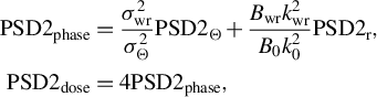 $$\begin{align}\mathrm{PSD}{2}_\mathrm{phase}&=\frac{\sigma_\mathrm{wr}^2}{\sigma_{\Theta}^2} \mathrm{PSD}{2}_{\Theta}+\frac{B_\mathrm{wr}{k}_\mathrm{wr}^2}{B_0{k}_0^2} \mathrm{PSD}{2}_\mathrm{r},\kern0.84em\nonumber\\\mathrm{PSD}{2}_\mathrm{dose}&=4 \mathrm{PSD}{2}_\mathrm{phase},\end{align}$$
where $\mathrm{PSD}{2}_{\Theta}$
is defined by Equations (37) and (36), and
$\mathrm{PSD}{2}_{\Theta}$
is defined by Equations (37) and (36), and $\mathrm{PSD}{2}_\mathrm{r}$
by Equation (40). Taking into account the linear relationship of
$\mathrm{PSD}{2}_\mathrm{r}$
by Equation (40). Taking into account the linear relationship of $\mathrm{PSD}1$
and
$\mathrm{PSD}1$
and $\mathrm{PSD}2$
in Equation (27), an expression for
$\mathrm{PSD}2$
in Equation (27), an expression for $\mathrm{PSD}1$
is analogous to Equation (43). The results presented in Sections 3–5 are summarized in Table 1, from which we obtain the final expression for the total
$\mathrm{PSD}1$
is analogous to Equation (43). The results presented in Sections 3–5 are summarized in Table 1, from which we obtain the final expression for the total $\mathrm{PSD}$
for one grating:
$\mathrm{PSD}$
for one grating:
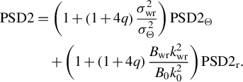 $$\begin{align}\mathrm{PSD}2&=\left(1+\left(1+4q\right)\frac{\sigma_\mathrm{wr}^2}{\sigma_{\Theta}^2}\right) \mathrm{PSD}{2}_{\Theta}\nonumber\\&\quad +\left(1+\left(1+4q\right)\frac{B_\mathrm{wr}{k}_\mathrm{wr}^2}{B_0{k}_0^2}\right) \mathrm{PSD}{2}_\mathrm{r}.\end{align}$$
By substituting Equation (44) into Equation (26) we obtain an expression for the contrast ${\mathbb{C}}_\mathrm{s}(t)$
for gratings G2 and G3, and the substitution of Equation (44) into Equation (29) gives an expression for the contrast
${\mathbb{C}}_\mathrm{s}(t)$
for gratings G2 and G3, and the substitution of Equation (44) into Equation (29) gives an expression for the contrast ${\mathbb{C}}_\mathrm{d}(t)$
for gratings G1 and G4, as well as for the mirrors on the input and output optics. Note that for the mirrors the expressions in parentheses in Equation (44) should be replaced by 1, since in this work we neglect fluctuations in the mirror reflectivity.
${\mathbb{C}}_\mathrm{d}(t)$
for gratings G1 and G4, as well as for the mirrors on the input and output optics. Note that for the mirrors the expressions in parentheses in Equation (44) should be replaced by 1, since in this work we neglect fluctuations in the mirror reflectivity. $\mathrm{PSD}$
for one grating (for a mirror, the columns ‘writing’ would contain zeros).
$\mathrm{PSD}$
for one grating (for a mirror, the columns ‘writing’ would contain zeros).

6 Example of contrast
$\mathbb{C}\left(\boldsymbol{t}\right)$
calculations

Above we considered the contrast introduced by one of the optical elements shown in Figure 1. In what follows we will assume that the total contrast is equal to the sum of the contrasts introduced by each element. This is obvious for obscurations and surface imperfections (both of the grating and of the mirror), since the obscurations are randomly located on different elements and the $\Theta \left(\boldsymbol{r}\right)$
functions of different elements are uncorrelated. The same applies to the roughness of beamline optics. For the contrast associated with writing the gratings, the issue is more complicated. It is reasonable to assume that all gratings are written under the same conditions; then their functions
$\Theta \left(\boldsymbol{r}\right)$
functions of different elements are uncorrelated. The same applies to the roughness of beamline optics. For the contrast associated with writing the gratings, the issue is more complicated. It is reasonable to assume that all gratings are written under the same conditions; then their functions $\mathcal{A}\left(\boldsymbol{r}\right)$
and
$\mathcal{A}\left(\boldsymbol{r}\right)$
and $\Delta \varphi \left(\boldsymbol{r}\right)$
are correlated. A strong correlation for
$\Delta \varphi \left(\boldsymbol{r}\right)$
are correlated. A strong correlation for $\Delta \varphi \left(\boldsymbol{r}\right)$
was measured in Ref. [Reference Kochetkov, Shaykin, Yakovlev, Khazanov, Cheplakov, Wang, Jin, Liu and Shao28]. However, since G2 and G3 (as well as G1 and G4) are mirror-like in the compressor, their identity is lost by virtue of the uncorrelated
$\Delta \varphi \left(\boldsymbol{r}\right)$
was measured in Ref. [Reference Kochetkov, Shaykin, Yakovlev, Khazanov, Cheplakov, Wang, Jin, Liu and Shao28]. However, since G2 and G3 (as well as G1 and G4) are mirror-like in the compressor, their identity is lost by virtue of the uncorrelated $\mathcal{A}\left(x,y\right)$
and
$\mathcal{A}\left(x,y\right)$
and $\mathcal{A}\left(-x,y\right)$
. For definiteness, we will assume that both the input and output optics consist of four mirrors. We will use the geometric parameters of the compressor from the XCELS project[
Reference Khazanov, Shaykin, Kostyukov, Ginzburg, Mukhin, Yakovlev, Soloviev, Kuznetsov, Mironov, Korzhimanov, Bulanov, Shaikin, Kochetkov, Kuzmin, Martyanov, Lozhkarev, Starodubtsev, Litvak and Sergeev
43
]; see Table 2.
$\mathcal{A}\left(-x,y\right)$
. For definiteness, we will assume that both the input and output optics consist of four mirrors. We will use the geometric parameters of the compressor from the XCELS project[
Reference Khazanov, Shaykin, Kostyukov, Ginzburg, Mukhin, Yakovlev, Soloviev, Kuznetsov, Mironov, Korzhimanov, Bulanov, Shaikin, Kochetkov, Kuzmin, Martyanov, Lozhkarev, Starodubtsev, Litvak and Sergeev
43
]; see Table 2.
Compressor parameters.
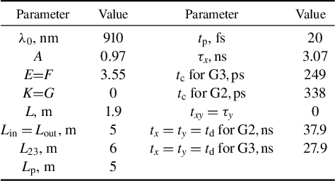
We have neither theoretical nor experimental data on the value of q, but we can make the following estimate. For the dispersion of the power reflectivity of the grating ${\sigma}_\mathrm{R}^2=2{\sigma}_\mathrm{a}^2$
, we obtain
${\sigma}_\mathrm{R}^2=2{\sigma}_\mathrm{a}^2$
, we obtain ${\sigma}_\mathrm{R}^2=8q{\sigma}_\mathrm{h}^2{B}_\mathrm{wr}{k}_\mathrm{wr}^2$
. We will take the minimum value of
${\sigma}_\mathrm{R}^2=8q{\sigma}_\mathrm{h}^2{B}_\mathrm{wr}{k}_\mathrm{wr}^2$
. We will take the minimum value of ${\sigma}_\mathrm{h}$
available in the literature, which at
${\sigma}_\mathrm{h}$
available in the literature, which at ${k}_\mathrm{h}=0.1/\mathrm{mm}$
is
${k}_\mathrm{h}=0.1/\mathrm{mm}$
is ${\sigma}_\mathrm{h}=0.38\;\mathrm{nm}$
[
Reference Hu, Wan, Jiang, Gu, Zhang, Jin, Liu, Zhao, Cao, Wei and Shao
54
]. Then at
${\sigma}_\mathrm{h}=0.38\;\mathrm{nm}$
[
Reference Hu, Wan, Jiang, Gu, Zhang, Jin, Liu, Zhao, Cao, Wei and Shao
54
]. Then at ${\lambda}_\mathrm{wr}=413\;\mathrm{nm}$
,
${\lambda}_\mathrm{wr}=413\;\mathrm{nm}$
, ${B}_\mathrm{wr}=3.7$
and
${B}_\mathrm{wr}=3.7$
and $q=1$
we obtain
$q=1$
we obtain ${\sigma}_\mathrm{R}=0.03$
, which is an unreasonably large value for such high-quality optics. For the National Ignition Facility (NIF) standard optics,
${\sigma}_\mathrm{R}=0.03$
, which is an unreasonably large value for such high-quality optics. For the National Ignition Facility (NIF) standard optics, ${\sigma}_\mathrm{h}=3.8\;\mathrm{nm}$
and
${\sigma}_\mathrm{h}=3.8\;\mathrm{nm}$
and ${\sigma}_\mathrm{R}=0.03$
is obtained at
${\sigma}_\mathrm{R}=0.03$
is obtained at $q=0.01$
. Although these estimates are very rough, we can conclude from them that
$q=0.01$
. Although these estimates are very rough, we can conclude from them that $q\ll 0.1$
and set
$q\ll 0.1$
and set $q=0$
in Equation (44). In other words, the impact of the writing optics imperfections on the fluctuations of the grating reflectivity may be neglected and only the diffracted wave phase fluctuations will be taken into account.
$q=0$
in Equation (44). In other words, the impact of the writing optics imperfections on the fluctuations of the grating reflectivity may be neglected and only the diffracted wave phase fluctuations will be taken into account.
The solid curves in Figure 5 show the PCR introduced by gratings G2 and G3, and the dotted curves show the PCR introduced by all the other optical elements taken together: gratings G1 and G4, as well as the input Min and output Mout optics. As stated above, such a partitioning is made because only gratings G2 and G3 have a spatial chirp $\left({\tau}_x\ne 0\right)$
and it is necessary to use either the exact Equation (25) or the approximate Equation (26), from which it follows that the cut-off time
$\left({\tau}_x\ne 0\right)$
and it is necessary to use either the exact Equation (25) or the approximate Equation (26), from which it follows that the cut-off time ${t}_\mathrm{c}$
in Equation (22) is 249 ps for G3 and 338 ps for G2, that is, there is both a pre-pulse and a post-pulse. There is no spatial chirp
${t}_\mathrm{c}$
in Equation (22) is 249 ps for G3 and 338 ps for G2, that is, there is both a pre-pulse and a post-pulse. There is no spatial chirp $\left({\tau}_x=0\right)$
on all the other elements, so one can use Equation (29), from which it follows that the cut-off time is zero, that is, there is no pre-pulse (if there is no negative diffraction, see Section 2).
$\left({\tau}_x=0\right)$
on all the other elements, so one can use Equation (29), from which it follows that the cut-off time is zero, that is, there is no pre-pulse (if there is no negative diffraction, see Section 2).
Contrast ${\mathbb{C}}_\mathrm{ob}(t)$
(red) and
${\mathbb{C}}_\mathrm{ob}(t)$
(red) and ${\mathbb{C}}_\mathrm{r}(t)$
(blue) for gratings G2 and G3 (solid curves), for other optical elements (dashed curves) and total contrast for the entire compressor (green dotted curve). Here, (a) and (b) differ only by the scale of the horizontal axis.
${\mathbb{C}}_\mathrm{r}(t)$
(blue) for gratings G2 and G3 (solid curves), for other optical elements (dashed curves) and total contrast for the entire compressor (green dotted curve). Here, (a) and (b) differ only by the scale of the horizontal axis.
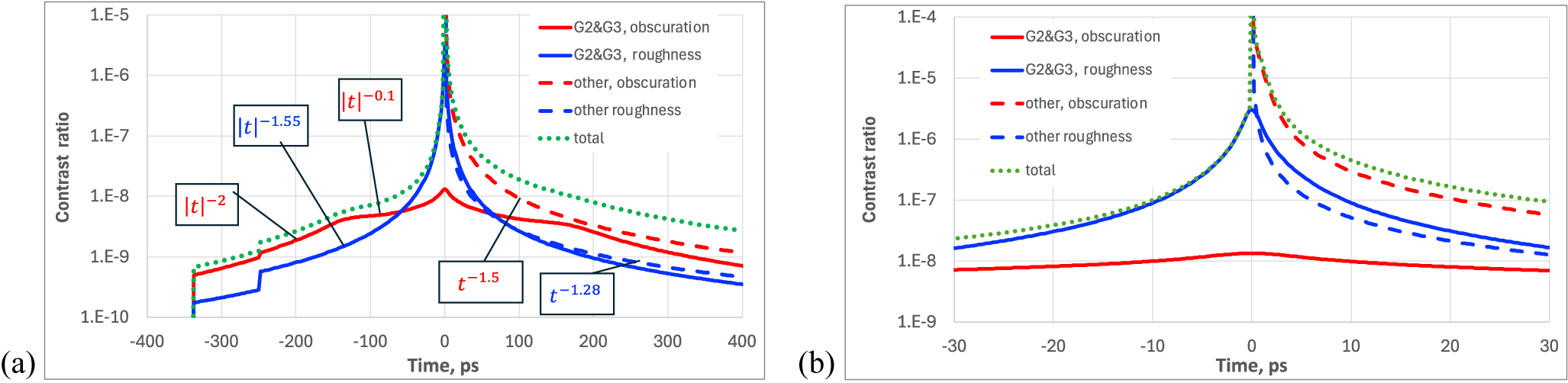
Schematic representation of the target illumination dynamics in the focal plane. (a) For gratings G2 and G3. (b) For all other optical elements depicted in Figure 1.
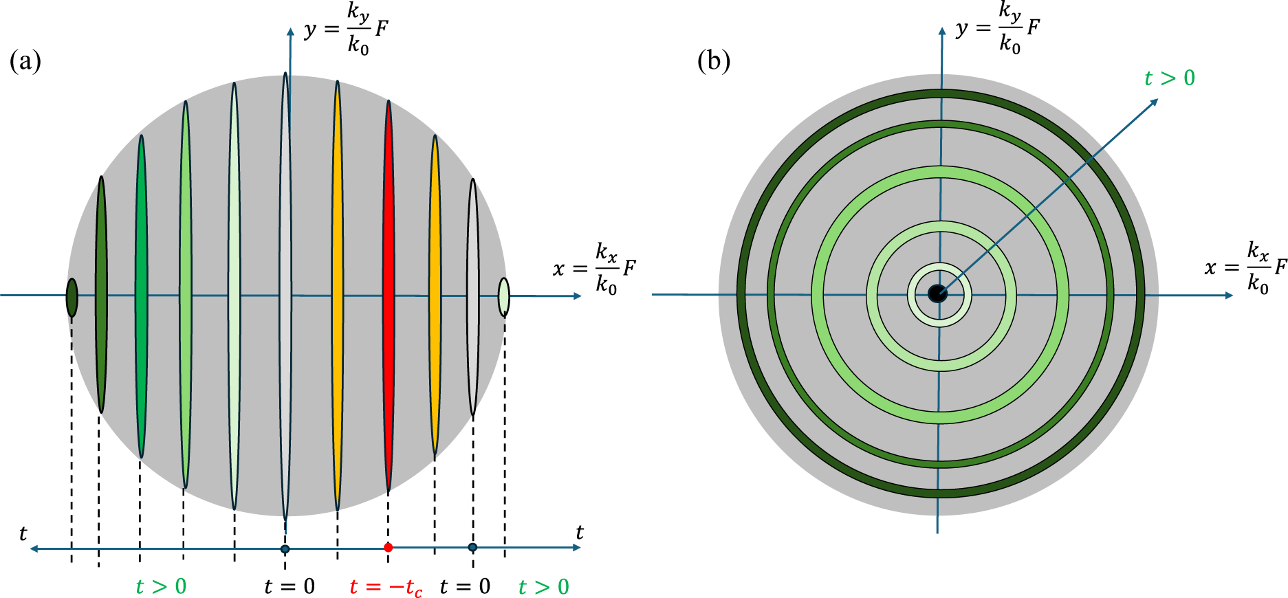
The red and blue curves in Figure 5 correspond to the contrast ${\mathbb{C}}_\mathrm{ob}(t)$
caused by obscurations and the contrast
${\mathbb{C}}_\mathrm{ob}(t)$
caused by obscurations and the contrast ${\mathbb{C}}_\mathrm{r}(t)$
caused by surface roughness. To obtain
${\mathbb{C}}_\mathrm{r}(t)$
caused by surface roughness. To obtain ${\mathbb{C}}_\mathrm{ob}(t),$
only the first term from Equation (44) (i.e., the term with
${\mathbb{C}}_\mathrm{ob}(t),$
only the first term from Equation (44) (i.e., the term with $\mathrm{PSD}{2}_{\Theta}$
from Equation (37)) should be substituted into Equations (25) and (29). The analysis shows that
$\mathrm{PSD}{2}_{\Theta}$
from Equation (37)) should be substituted into Equations (25) and (29). The analysis shows that ${\mathbb{C}}_\mathrm{ob}(t)$
is almost independent of Z; it depends only on two dimensionless quantities –
${\mathbb{C}}_\mathrm{ob}(t)$
is almost independent of Z; it depends only on two dimensionless quantities – $\xi$
and
$\xi$
and ${k}_0{w}_\mathrm{min}$
. Further, we will assume that
${k}_0{w}_\mathrm{min}$
. Further, we will assume that ${w}_\mathrm{min}=0.25\;\mathrm{mm}$
,
${w}_\mathrm{min}=0.25\;\mathrm{mm}$
, $\xi =3.9$
[
Reference Spaeth, Manes, Widmayer, Williams, Whitman, Henesian, Stowers and Honig
23
] and that the compressor has already been used in a large number of shots, as a result of which grating G4 and the output optics ‘accumulated’ obscurations in the amount measured in Ref. [Reference Spaeth, Manes, Widmayer, Williams, Whitman, Henesian, Stowers and Honig23], which corresponds to
$\xi =3.9$
[
Reference Spaeth, Manes, Widmayer, Williams, Whitman, Henesian, Stowers and Honig
23
] and that the compressor has already been used in a large number of shots, as a result of which grating G4 and the output optics ‘accumulated’ obscurations in the amount measured in Ref. [Reference Spaeth, Manes, Widmayer, Williams, Whitman, Henesian, Stowers and Honig23], which corresponds to ${\sigma}_{\Theta}^2=6.1\times {10}^{-4}$
. The input optics, gratings G1–G3 and writing optics are not exposed to powerful femtosecond radiation, so we will assume that for them
${\sigma}_{\Theta}^2=6.1\times {10}^{-4}$
. The input optics, gratings G1–G3 and writing optics are not exposed to powerful femtosecond radiation, so we will assume that for them ${\sigma}_{\Theta}^2=6.1\times {10}^{-6}$
, that is, it is 100 times smaller. We remind the reader that
${\sigma}_{\Theta}^2=6.1\times {10}^{-6}$
, that is, it is 100 times smaller. We remind the reader that ${\sigma}_{\Theta}^2$
is equal to the fraction of the surface occupied by obscurations, as well as to the fraction of the noise energy
${\sigma}_{\Theta}^2$
is equal to the fraction of the surface occupied by obscurations, as well as to the fraction of the noise energy ${W}_{\Theta}/{W}_0$
; see Section 2.
${W}_{\Theta}/{W}_0$
; see Section 2.
To obtain ${\mathbb{C}}_\mathrm{r}(t)$
, it is necessary to substitute into Equations (25) and (29) only the second term from Equation (44) (the term with
${\mathbb{C}}_\mathrm{r}(t)$
, it is necessary to substitute into Equations (25) and (29) only the second term from Equation (44) (the term with $\mathrm{PSD}{2}_\mathrm{r}$
from Equation (40)). The analysis of these expressions shows that
$\mathrm{PSD}{2}_\mathrm{r}$
from Equation (40)). The analysis of these expressions shows that ${\mathbb{C}}_\mathrm{r}(t)$
depends only on two dimensionless quantities –
${\mathbb{C}}_\mathrm{r}(t)$
depends only on two dimensionless quantities – $a$
and
$a$
and ${\sigma}_\mathrm{r}^2={B}_0{k}_0^2{\sigma}_\mathrm{h}^2{\left({k}_\mathrm{h}/{k}_0\right)}^{a-2}$
, with the dependence on
${\sigma}_\mathrm{r}^2={B}_0{k}_0^2{\sigma}_\mathrm{h}^2{\left({k}_\mathrm{h}/{k}_0\right)}^{a-2}$
, with the dependence on ${\sigma}_\mathrm{r}^2$
being linear. In other words, for a fixed a, the shape of
${\sigma}_\mathrm{r}^2$
being linear. In other words, for a fixed a, the shape of ${\mathbb{C}}_\mathrm{r}(t)$
does not change. Further, we will assume that
${\mathbb{C}}_\mathrm{r}(t)$
does not change. Further, we will assume that $a=2.55$
, and
$a=2.55$
, and ${\sigma}_\mathrm{h}^2$
of all optical elements, including mirrors used for writing the gratings (see Figure 4), is 200 times less than the data in Ref. [Reference Camus, Coic, Blanchot, Bouillet, Lavastre, Mangeant, Rouyer and Néauport55], 10 times less than the NIF standard[
Reference Spaeth, Manes, Widmayer, Williams, Whitman, Henesian, Stowers and Honig
23
], but 10 times more than the data reported in Ref. [Reference Hu, Wan, Jiang, Gu, Zhang, Jin, Liu, Zhao, Cao, Wei and Shao54]. At
${\sigma}_\mathrm{h}^2$
of all optical elements, including mirrors used for writing the gratings (see Figure 4), is 200 times less than the data in Ref. [Reference Camus, Coic, Blanchot, Bouillet, Lavastre, Mangeant, Rouyer and Néauport55], 10 times less than the NIF standard[
Reference Spaeth, Manes, Widmayer, Williams, Whitman, Henesian, Stowers and Honig
23
], but 10 times more than the data reported in Ref. [Reference Hu, Wan, Jiang, Gu, Zhang, Jin, Liu, Zhao, Cao, Wei and Shao54]. At ${k}_\mathrm{h}=0.1/\mathrm{mm}$
this corresponds to
${k}_\mathrm{h}=0.1/\mathrm{mm}$
this corresponds to ${\sigma}_\mathrm{h}\approx 1.2\;\mathrm{nm}$
. It is easy to show that the fraction of the noise energy
${\sigma}_\mathrm{h}\approx 1.2\;\mathrm{nm}$
. It is easy to show that the fraction of the noise energy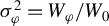 ${\sigma}_{\varphi}^2={W}_{\varphi}/{W}_0$
caused by scattering on a rough surface is equal to
${\sigma}_{\varphi}^2={W}_{\varphi}/{W}_0$
caused by scattering on a rough surface is equal to ${\sigma}_\mathrm{h}^2{B}_0{k}_0^2$
and at
${\sigma}_\mathrm{h}^2{B}_0{k}_0^2$
and at ${B}_0=2.8$
we obtain
${B}_0=2.8$
we obtain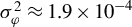 ${\sigma}_{\varphi}^2\approx 1.9\times {10}^{-4}$
. This is approximately 30 times more than
${\sigma}_{\varphi}^2\approx 1.9\times {10}^{-4}$
. This is approximately 30 times more than ${\sigma}_{\Theta}^2=6.1\times {10}^{-6}$
presented above. However, at long times
${\sigma}_{\Theta}^2=6.1\times {10}^{-6}$
presented above. However, at long times ${\mathbb{C}}_\mathrm{r}\ll {\mathbb{C}}_\mathrm{ob}$
, since
${\mathbb{C}}_\mathrm{r}\ll {\mathbb{C}}_\mathrm{ob}$
, since ${\mathbb{C}}_\mathrm{ob}$
decreases very slowly. As a result, at long times the total PCR is determined by
${\mathbb{C}}_\mathrm{ob}$
decreases very slowly. As a result, at long times the total PCR is determined by ${\mathbb{C}}_\mathrm{ob},$
and at short times by
${\mathbb{C}}_\mathrm{ob},$
and at short times by ${\mathbb{C}}_\mathrm{r}$
. This qualitative conclusion is valid for a wide range of
${\mathbb{C}}_\mathrm{r}$
. This qualitative conclusion is valid for a wide range of ${\sigma}_{\varphi}^2$
and
${\sigma}_{\varphi}^2$
and ${\sigma}_{\Theta}^2$
. Any quantitative comparison of
${\sigma}_{\Theta}^2$
. Any quantitative comparison of ${\mathbb{C}}_\mathrm{ob}$
and
${\mathbb{C}}_\mathrm{ob}$
and ${\mathbb{C}}_\mathrm{r}$
strongly depends on the quality of the optical elements, because
${\mathbb{C}}_\mathrm{r}$
strongly depends on the quality of the optical elements, because ${\mathbb{C}}_{\mathrm{ob},\mathrm{r}}$
are proportional to
${\mathbb{C}}_{\mathrm{ob},\mathrm{r}}$
are proportional to ${\sigma}_{\Theta, \varphi}^2$
and the
${\sigma}_{\Theta, \varphi}^2$
and the ${\sigma}_{\varphi}^2/{\sigma}_{\Theta}^2$
ratio can vary over a wide range in practice. For example, the boundary is the instant of time at which
${\sigma}_{\varphi}^2/{\sigma}_{\Theta}^2$
ratio can vary over a wide range in practice. For example, the boundary is the instant of time at which ${\mathbb{C}}_\mathrm{r}={\mathbb{C}}_\mathrm{ob}$
is
${\mathbb{C}}_\mathrm{r}={\mathbb{C}}_\mathrm{ob}$
is ${t}_{\ast }=-60\;\mathrm{ps}$
in Figure 5(a). If the optics roughness
${t}_{\ast }=-60\;\mathrm{ps}$
in Figure 5(a). If the optics roughness ${\sigma}_{\varphi}^2$
increases by a factor of 10,
${\sigma}_{\varphi}^2$
increases by a factor of 10, ${\mathbb{C}}_\mathrm{r}$
also increases by a factor of 10 and
${\mathbb{C}}_\mathrm{r}$
also increases by a factor of 10 and ${t}_{\ast }=-12\;\mathrm{ps}$
.
${t}_{\ast }=-12\;\mathrm{ps}$
.
The small deviation of the contrast from parity observed in Figure 5 for curves G2 and G3 constructed according to Equation (25) may be neglected in practice and a simpler Equation (26) can be used instead of Equation (25), that is, $\mathbb{C}(t)$
is proportional to
$\mathbb{C}(t)$
is proportional to $\mathrm{PSD}1\left({k}_x\right)$
and the mapping is linear:
$\mathrm{PSD}1\left({k}_x\right)$
and the mapping is linear: $t={\tau}_x{k}_x/{k}_0$
. Since in the focal plane the distance from the beam axis (along the x-axis) is
$t={\tau}_x{k}_x/{k}_0$
. Since in the focal plane the distance from the beam axis (along the x-axis) is $x=F{k}_x/{k}_0$
, then for the pre-pulse,
$x=F{k}_x/{k}_0$
, then for the pre-pulse, $x$
is related to the time of its appearance on the target as
$x$
is related to the time of its appearance on the target as $x= Ft/{\tau}_x$
. Thus, the radiation reaches the target at the time
$x= Ft/{\tau}_x$
. Thus, the radiation reaches the target at the time $t=-{t}_{\mathrm{c}}$
, illuminating a vertical strip at a distance
$t=-{t}_{\mathrm{c}}$
, illuminating a vertical strip at a distance $x=F{t}_{\mathrm{c}}/{\tau}_x$
; see Figure 6(a). Then this strip splits into two and its replicas move in opposite directions at speed
$x=F{t}_{\mathrm{c}}/{\tau}_x$
; see Figure 6(a). Then this strip splits into two and its replicas move in opposite directions at speed $F/{\tau}_x$
. At
$F/{\tau}_x$
. At $t=0$
, one of them reaches the axis and continues to move in the same direction at the same speed. The intensity and, hence, the fluence change proportionally to
$t=0$
, one of them reaches the axis and continues to move in the same direction at the same speed. The intensity and, hence, the fluence change proportionally to $\mathbb{C}(t)$
. For any given fluence value (for example, at which the target is destroyed), this simple reasoning allows us to calculate for each point of the target the time at which this value will be reached.
$\mathbb{C}(t)$
. For any given fluence value (for example, at which the target is destroyed), this simple reasoning allows us to calculate for each point of the target the time at which this value will be reached.
For all the other optical elements, except for G2 and G3, PCR $\mathbb{C}(t)$
is proportional to
$\mathbb{C}(t)$
is proportional to $\mathrm{PSD}2\left({k}_{\perp}\right)$
in Equation (29) and the mapping is quadratic:
$\mathrm{PSD}2\left({k}_{\perp}\right)$
in Equation (29) and the mapping is quadratic: $t={t}_\mathrm{d}{k}_{\perp}^2/{k}_0^2$
. The radiation reaches the target at
$t={t}_\mathrm{d}{k}_{\perp}^2/{k}_0^2$
. The radiation reaches the target at $t=0$
, exactly at the beam axis. At all subsequent instants of time, the radiation illuminates a ring of radius
$t=0$
, exactly at the beam axis. At all subsequent instants of time, the radiation illuminates a ring of radius $r=F{k}_{\perp }/{k}_0=F\sqrt{t/{t}_\mathrm{d}}$
, which increases in proportion to
$r=F{k}_{\perp }/{k}_0=F\sqrt{t/{t}_\mathrm{d}}$
, which increases in proportion to $\sqrt{t}$
(Figure 6(b)).
$\sqrt{t}$
(Figure 6(b)).
The laws of $\mathbb{C}(t)$
decrease are different; see Figure 5(a). The
$\mathbb{C}(t)$
decrease are different; see Figure 5(a). The ${\mathbb{C}}_\mathrm{ob}(t)$
curve for G2 and G3 clearly features the boundary between the two ranges, in which the law of
${\mathbb{C}}_\mathrm{ob}(t)$
curve for G2 and G3 clearly features the boundary between the two ranges, in which the law of ${\mathbb{C}}_\mathrm{ob}(t)$
decrease changes from
${\mathbb{C}}_\mathrm{ob}(t)$
decrease changes from ${\left|t\right|}^{-0.1}$
to
${\left|t\right|}^{-0.1}$
to ${\left|t\right|}^{-2}$
. Unfortunately, quantitative comparison with the experiments is impossible due to lack of PSD functions for the gratings and optics used in the experiments. There is a good qualitative agreement between
${\left|t\right|}^{-2}$
. Unfortunately, quantitative comparison with the experiments is impossible due to lack of PSD functions for the gratings and optics used in the experiments. There is a good qualitative agreement between ${\mathbb{C}}_\mathrm{ob}(t)$
and the results of measurements[
Reference Roeder, Zobus, Major and Bagnoud
11
], where a plateau (an area where
${\mathbb{C}}_\mathrm{ob}(t)$
and the results of measurements[
Reference Roeder, Zobus, Major and Bagnoud
11
], where a plateau (an area where ${\mathbb{C}}_\mathrm{ob}(t)\sim {\left|t\right|}^{-0.1}$
) caused by scattering at stretcher mirrors, which is equivalent to scattering at gratings G2 and G3[
Reference Khazanov
22
], was also observed. The theory (in particular the dotted curve in Figure 5) explains the frequently observed experimental asymmetry of the contrast: the post-pulse is larger than the pre-pulse[
Reference Webb, Dorrer, Bahk, Jeon, Roides and Bromage
5
,
Reference Hooker, Tang, Chekhlov, Collier, Divall, Ertel, Hawkes, Parry and Rajeev
15
–
Reference Lu, Zhang, Li and Leng
18
,
Reference Wang, Liu, Lu, Chen, Long, Li, Chen, Chen, Bai, Li, Peng, Liu, Wu, Wang, Li, Xu, Liang, Leng and Li
46
,
Reference Khodakovskiy, Kalashnikov, Gontier, Falcoz and Paul
47
]. Also, Figure 5(a) shows the typical ‘triangular’
${\mathbb{C}}_\mathrm{ob}(t)\sim {\left|t\right|}^{-0.1}$
) caused by scattering at stretcher mirrors, which is equivalent to scattering at gratings G2 and G3[
Reference Khazanov
22
], was also observed. The theory (in particular the dotted curve in Figure 5) explains the frequently observed experimental asymmetry of the contrast: the post-pulse is larger than the pre-pulse[
Reference Webb, Dorrer, Bahk, Jeon, Roides and Bromage
5
,
Reference Hooker, Tang, Chekhlov, Collier, Divall, Ertel, Hawkes, Parry and Rajeev
15
–
Reference Lu, Zhang, Li and Leng
18
,
Reference Wang, Liu, Lu, Chen, Long, Li, Chen, Chen, Bai, Li, Peng, Liu, Wu, Wang, Li, Xu, Liang, Leng and Li
46
,
Reference Khodakovskiy, Kalashnikov, Gontier, Falcoz and Paul
47
]. Also, Figure 5(a) shows the typical ‘triangular’ $\mathbb{C}(t)$
shapes observed in many experiments[
Reference Webb, Dorrer, Bahk, Jeon, Roides and Bromage
5
,
Reference Schanz, Roth and Bagnoud
8
,
Reference Roeder, Zobus, Major and Bagnoud
11
,
Reference Ranc, Blanc, Lebas, Martin, Zou, Mathieu, Radier, Ricaud, Druon and Papadopoulos
14
–
Reference Roeder, Zobus, Brabetz and Bagnoud
19
,
Reference Khodakovskiy, Kalashnikov, Gontier, Falcoz and Paul
47
].
$\mathbb{C}(t)$
shapes observed in many experiments[
Reference Webb, Dorrer, Bahk, Jeon, Roides and Bromage
5
,
Reference Schanz, Roth and Bagnoud
8
,
Reference Roeder, Zobus, Major and Bagnoud
11
,
Reference Ranc, Blanc, Lebas, Martin, Zou, Mathieu, Radier, Ricaud, Druon and Papadopoulos
14
–
Reference Roeder, Zobus, Brabetz and Bagnoud
19
,
Reference Khodakovskiy, Kalashnikov, Gontier, Falcoz and Paul
47
].
Despite the larger number of elements (two gratings and eight mirrors), the ${\mathbb{C}}_\mathrm{r}(t)$
value for G2 and G3 is close to the
${\mathbb{C}}_\mathrm{r}(t)$
value for G2 and G3 is close to the ${\mathbb{C}}_\mathrm{r}(t)$
value for all the other elements. The point is that the contribution of
${\mathbb{C}}_\mathrm{r}(t)$
value for all the other elements. The point is that the contribution of ${\mathbb{C}}_\mathrm{r}(t)$
for gratings is much larger than for mirrors, since in mirrors there is no dominant (due to
${\mathbb{C}}_\mathrm{r}(t)$
for gratings is much larger than for mirrors, since in mirrors there is no dominant (due to ${k}_\mathrm{wr}^2\gg {k}_0^2$
) contribution from writing optics.
${k}_\mathrm{wr}^2\gg {k}_0^2$
) contribution from writing optics.
For the PCR caused by the roughness of gratings and mirrors of the input and output optics, generalizations to advanced compressors and stretchers were proposed in Ref. [Reference Khazanov22]. Without repeating them here, we just note that they are valid for all the results obtained above, since they are based on the Equation (19) in Ref. [Reference Khazanov22], which coincides with Equation (17) if $\mathrm{PSD}{2}_{\varphi}\left({\boldsymbol{k}}_{\boldsymbol{\perp}}\right)$
is replaced by
$\mathrm{PSD}{2}_{\varphi}\left({\boldsymbol{k}}_{\boldsymbol{\perp}}\right)$
is replaced by $\mathrm{PSD}2\left({\boldsymbol{k}}_{\boldsymbol{\perp}}\right)$
.
$\mathrm{PSD}2\left({\boldsymbol{k}}_{\boldsymbol{\perp}}\right)$
.
7 Conclusion
In the paraxial approximation, with allowance for all orders of dispersion, the problem of the impact of imperfect compressor gratings and transport optics on the PCR $\mathbb{C}(t)$
in Equation (1) of a femtosecond laser pulse has been solved. All types of imperfections have been considered: non-flat surface profile (roughness) and dirt/damage/obscuration on the surface, as well as roughness and obscuration on the optics used to write holographic gratings. The analytically obtained Equation (25) for
$\mathbb{C}(t)$
in Equation (1) of a femtosecond laser pulse has been solved. All types of imperfections have been considered: non-flat surface profile (roughness) and dirt/damage/obscuration on the surface, as well as roughness and obscuration on the optics used to write holographic gratings. The analytically obtained Equation (25) for $\mathbb{C}(t)$
is valid for any optical element, for both the Treacy compressor and the out-of-plane compressor. For finding
$\mathbb{C}(t)$
is valid for any optical element, for both the Treacy compressor and the out-of-plane compressor. For finding $\mathbb{C}(t)$
it is sufficient to know the PSD of the field reflected from an imperfect optical element. For the roughness, the field PSD is determined by the PSD of the surface profile and, for the obscuration, by the obtained Equation (36).
$\mathbb{C}(t)$
it is sufficient to know the PSD of the field reflected from an imperfect optical element. For the roughness, the field PSD is determined by the PSD of the surface profile and, for the obscuration, by the obtained Equation (36).
Strictly speaking, the PCR caused by the imperfections of the second and third gratings is not an even function of time, since diffraction results in the cut-off time ${t}_\mathrm{c}$
,
${t}_\mathrm{c}$
, $\mathbb{C}\left(t<-{t}_\mathrm{c}\right)=0$
, as well as in a small deviation from parity at
$\mathbb{C}\left(t<-{t}_\mathrm{c}\right)=0$
, as well as in a small deviation from parity at $\left|t\right|<{t}_\mathrm{c}$
. However, this deviation is small and can be neglected in practice. Then
$\left|t\right|<{t}_\mathrm{c}$
. However, this deviation is small and can be neglected in practice. Then $\mathbb{C}(t)$
is proportional to
$\mathbb{C}(t)$
is proportional to $\mathrm{PSD}1\left({k}_x\right)$
of the reflected field in Equation (26), with the arguments of these functions being related linearly as
$\mathrm{PSD}1\left({k}_x\right)$
of the reflected field in Equation (26), with the arguments of these functions being related linearly as $t={\tau}_x{k}_x/{k}_0$
. The radiation scattered by the second and third gratings arrives at the target at the time
$t={\tau}_x{k}_x/{k}_0$
. The radiation scattered by the second and third gratings arrives at the target at the time $t=-{t}_{\mathrm{c}}$
, illuminating a vertical stripe at distance
$t=-{t}_{\mathrm{c}}$
, illuminating a vertical stripe at distance $x=F{t}_{\mathrm{c}}/{\tau}_x$
(Figure 6(a)). Then this stripe bifurcates and its replicas move in opposite directions at a speed
$x=F{t}_{\mathrm{c}}/{\tau}_x$
(Figure 6(a)). Then this stripe bifurcates and its replicas move in opposite directions at a speed $F/{\tau}_x$
. One of them, at the time of the main pulse arrival
$F/{\tau}_x$
. One of them, at the time of the main pulse arrival $\left(t=0\right)$
, reaches the beam axis and continues to move in the same direction at the same speed.
$\left(t=0\right)$
, reaches the beam axis and continues to move in the same direction at the same speed.
The PCR caused by imperfections of all the other optical elements, except for the second and third gratings, is nonzero only at $t>0$
. This radiation reaches the target at
$t>0$
. This radiation reaches the target at $t=0$
exactly on the beam axis and further moves away from the axis like a circle on water from a thrown stone. Here,
$t=0$
exactly on the beam axis and further moves away from the axis like a circle on water from a thrown stone. Here, $\mathbb{C}(t)$
is proportional to the
$\mathbb{C}(t)$
is proportional to the $\mathrm{PSD}2\left({k}_{\perp}\right)$
of the reflected field in Equation (29), with the arguments of these functions being related quadratically:
$\mathrm{PSD}2\left({k}_{\perp}\right)$
of the reflected field in Equation (29), with the arguments of these functions being related quadratically: $t={t}_\mathrm{d}{k}_{\perp}^2/{k}_0^2$
. It is the scattering on other optical elements that explains the contrast asymmetry observed in the experiment when the sign of the time is changed.
$t={t}_\mathrm{d}{k}_{\perp}^2/{k}_0^2$
. It is the scattering on other optical elements that explains the contrast asymmetry observed in the experiment when the sign of the time is changed.
With the same roughness and the same obscuration, the contribution to the PCR of the optics used to write holographic gratings is significantly greater than the contribution of the gratings themselves. This is due to the fact that shorter-wave radiation is used for writing, and the phase distortions are proportional to ${\lambda}^{-1}$
.
${\lambda}^{-1}$
.
The comparison of ${\mathbb{C}}_\mathrm{ob}(t)$
caused by obscurations and
${\mathbb{C}}_\mathrm{ob}(t)$
caused by obscurations and ${\mathbb{C}}_\mathrm{r}(t)$
caused by roughness shows that, at small
${\mathbb{C}}_\mathrm{r}(t)$
caused by roughness shows that, at small $t,$
$t,$ ${\mathbb{C}}_\mathrm{r}(t)$
prevails and at large
${\mathbb{C}}_\mathrm{r}(t)$
prevails and at large $t,$
$t,$ ${\mathbb{C}}_\mathrm{ob}(t),$
since its distinctive feature is a very slow decrease with increasing
${\mathbb{C}}_\mathrm{ob}(t),$
since its distinctive feature is a very slow decrease with increasing $\left|t\right|$
(Figure 5(a)). The instant of time at which
$\left|t\right|$
(Figure 5(a)). The instant of time at which ${\mathbb{C}}_\mathrm{ob}(t)={\mathbb{C}}_\mathrm{r}(t)$
strongly depends on the proportion of the radiation power scattered on obscuration and on roughness.
${\mathbb{C}}_\mathrm{ob}(t)={\mathbb{C}}_\mathrm{r}(t)$
strongly depends on the proportion of the radiation power scattered on obscuration and on roughness.
Acknowledgements
This work was supported by the Ministry of Science and Higher Education of the Russian Federation (Project No. FFUF-2025-0011).
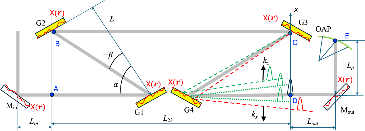

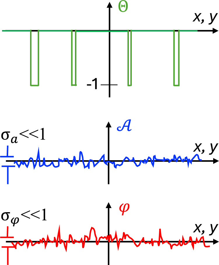

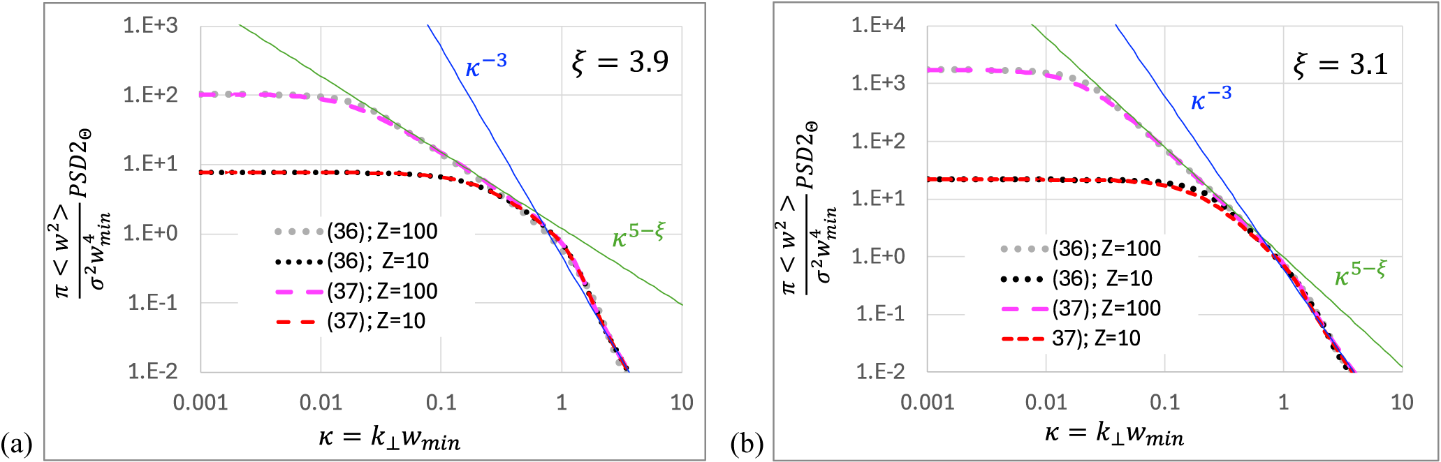


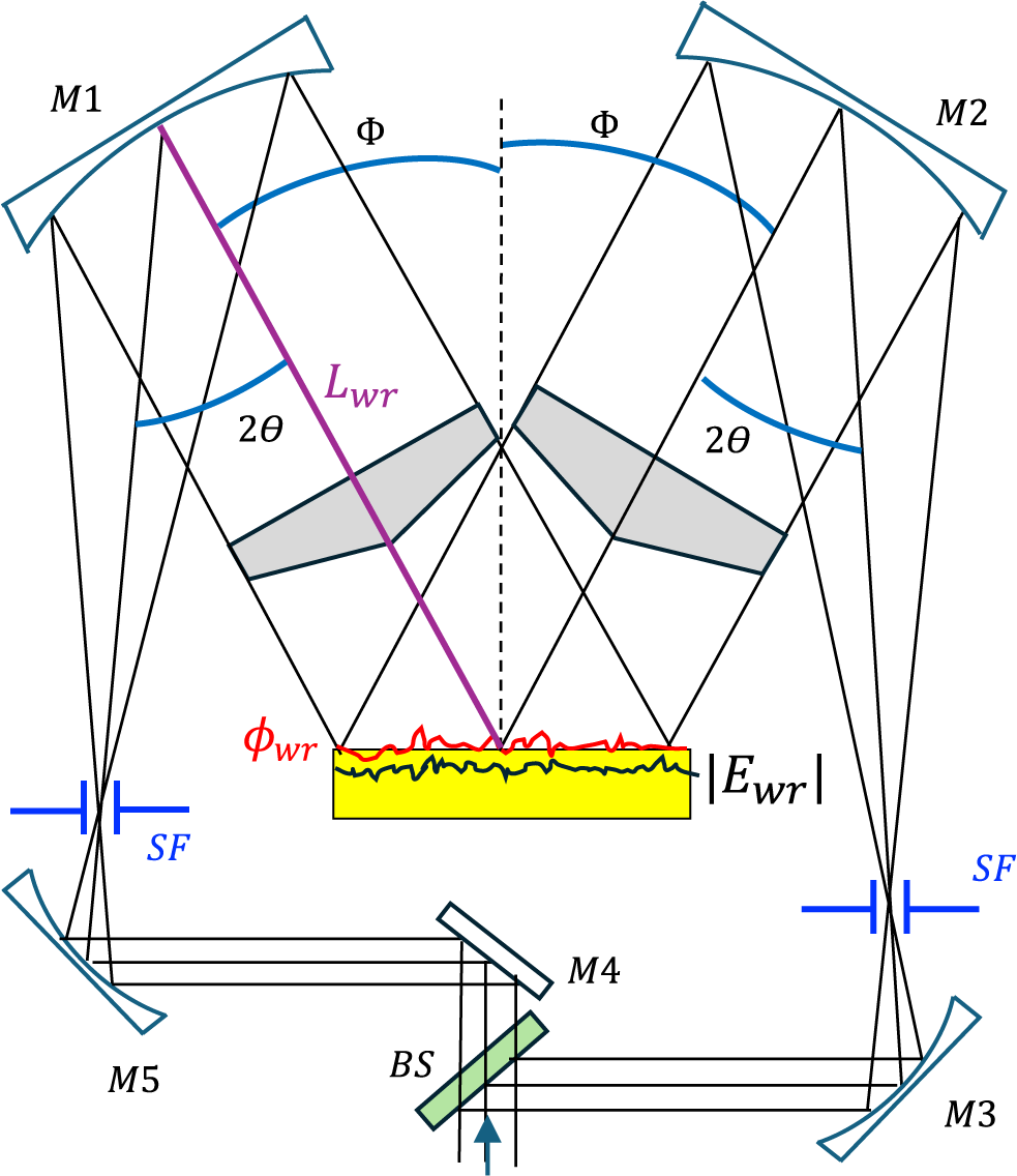


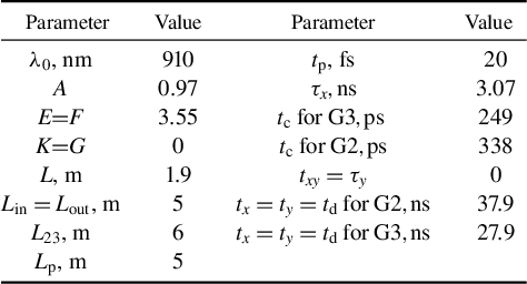
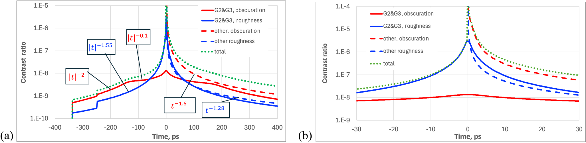


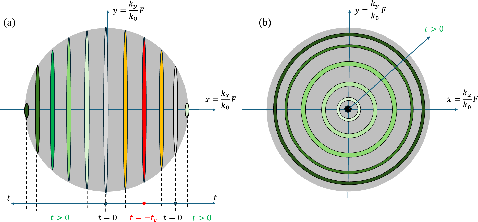

 Open access

