


1 Introduction
The subject of this study, a flowing film of fluid contacting a surface with complex topographic patterns, is a prominent feature of both technology and nature. Superhydrophobic surfaces (SHS) (Choi et al. Reference Choi, Ulmanella, Kim, Ho and Kim2006; Ybert et al. Reference Ybert, Barentin, Cottin-Bizonne, Joseph and Bocquet2007; Zhou et al. Reference Zhou, Asmolov, Schmid and Vinogradova2013; Song, Daniello & Rothstein Reference Song, Daniello and Rothstein2014) and liquid-impregnated surfaces (LIS) (Wexler, Jacobi & Stone Reference Wexler, Jacobi and Stone2015; Asmolov, Nizkaya & Vinogradova Reference Asmolov, Nizkaya and Vinogradova2018; Solomon et al. Reference Solomon, Chen, Rapoport, Helal, McKinley, Chiang and Varanasi2018) have been shown to reduce the frictional resistance of flow passages with potential applications to microfluidics and flow batteries. An important application of SHS and LIS in the form of antimicrobial surfaces for implants and surgical instruments involve contact with flowing blood (Wong et al. Reference Wong, Kang, Tang, Smythe, Hatton, Grinthal and Aizenberg2011; Parmar et al. Reference Parmar, Kumar, Sankar, Datta, Prakash, Mohanty and Kalyanasundaram2018). Similarly, contact with flowing sea water may arise in applications of SHS and LIS to prevent marine bio-fouling (Ware et al. Reference Ware, Smith-Palmer, Peppou-Chapman, Scarratt, Humphries, Balzer and Neto2018). In fact, the stability of LIS under shear is a specific area of concern (Wexler et al. Reference Wexler, Jacobi and Stone2015) for their technological viability. The anisotropy of flow over topographic patterns can be leveraged to successfully mix reagents in microfluidics (Stroock & McGraw Reference Stroock and McGraw2004) and even to effect separations (Asmolov et al. Reference Asmolov, Dubov, Nizkaya, Kuehne and Vinogradova2015).
In addition to relevance to the above-discussed more recent technological advances, a substantial motivation behind studying wetted topographic patterns has historically been in the realm of reduction of skin-friction drag in turbulent flows through riblets immersed within the viscous sublayer (Bechert & Bartenwerfer Reference Bechert and Bartenwerfer1989; Luchini, Manzo & Pozzi Reference Luchini, Manzo and Pozzi1991; Choi, Moin & Kim Reference Choi, Moin and Kim1993; Chang et al. Reference Chang, Jung, Choi and Kim2019). Inspiration for this application is drawn from the micro-structure of the skin of marine organisms like fast-moving sharks. Also of relevance to the current study on confined flows is the fact that fractured rocks in natural/man-made geological formations also present complex topographies to even the laminar flow of oil and water, causing departures from the Poiseuille law that need careful consideration (Sisavath et al. Reference Sisavath, Al-Yaarubi, Pain and Zimmerman2003).
Corrugations provide often the smallest or the least-resolvable scale in the hierarchy of scales that affect fluid flow (Bechert & Bartenwerfer Reference Bechert and Bartenwerfer1989; Miksis & Davis Reference Miksis and Davis1994; Tuck & Kouzoubov Reference Tuck and Kouzoubov1995; Kamrin, Bazant & Stone Reference Kamrin, Bazant and Stone2010). A powerful theoretical paradigm in the assessment of the hydrodynamic effects of wall corrugation arises from the realization that the feature-averaged effects of wall corrugations accessible to coarse-scale measurements can be quantified easily through effective equation approaches such as locating an effective no-slip plane (Tuck & Kouzoubov Reference Tuck and Kouzoubov1995; Kamrin et al. Reference Kamrin, Bazant and Stone2010) or evaluating for confined flows the hydrodynamic conductance of an equivalent channel with a simpler wall geometry (Stroock et al. Reference Stroock, Dertinger, Whitesides and Ajdari2002; Feuillebois, Bazant & Vinogradova Reference Feuillebois, Bazant and Vinogradova2009). The location of the effective no-slip plane, which depends of course on the reference plane for measuring distances, has been specified variously through closely related parameters such as the ‘effective slip length’ or the ‘protrusion height’, the latter term being used almost exclusively in the turbulent-drag-reduction literature (Bechert & Bartenwerfer Reference Bechert and Bartenwerfer1989). In what follows, the above-discussed effective equation approach will play an important role.
In SHS, the liquid does not contact all points of the pattern and the details of the solid-contacting gas flow is not usually resolved (Lauga & Stone Reference Lauga and Stone2003; Asmolov et al. Reference Asmolov, Schmieschek, Harting and Vinogradova2013a ; Kumar, Datta & Kalyanasundaram Reference Kumar, Datta and Kalyanasundaram2016). In contrast, the current study will deal with a fluid contacting a solid no-slip surface. Crucially, in creeping flow, SHS (Zhou et al. Reference Zhou, Asmolov, Schmid and Vinogradova2013) and wetted surfaces (Lecoq et al. Reference Lecoq, Anthore, Cichocki, Szymczak and Feuillebois2004) with the same pattern waveform (e.g. trapezoidal, as in the above two studies) act as drag-reducing and drag-enhancing surfaces, respectively, as judged from the location of the effective no-slip plane, which is closer to the troughs in SHS and closer to the peaks in wetted surfaces. Wetted trapezoidal surfaces such as in Lecoq et al. (Reference Lecoq, Anthore, Cichocki, Szymczak and Feuillebois2004) will be investigated as an application in the current study. The literature on SHS will not, therefore, be surveyed in great detail. The literature on channels with non-planar mean wall shapes will also be left out of scope.
The problem of predicting the location of the effective no-slip plane in shear flows bounded only on one side by a specialized topography such as rectangular or sinusoidal topographic patterns has attracted the attention of several researchers over last half a century (Richardson Reference Richardson1973; Hocking Reference Hocking1976; Tuck & Kouzoubov Reference Tuck and Kouzoubov1995; Wang Reference Wang2003, Reference Wang2010; Dewangan & Datta Reference Dewangan and Datta2019). Unconfined flows with trapezoidal, triangular and other cornered topographies having specialized analytical forms have been accessed through conformal mapping (Bechert & Bartenwerfer Reference Bechert and Bartenwerfer1989) and semi-analytical approaches such as those based on boundary integral formulations (Luchini et al. Reference Luchini, Manzo and Pozzi1991; Wang Reference Wang2003) and spectral-asymptotic analyses (Lecoq et al. Reference Lecoq, Anthore, Cichocki, Szymczak and Feuillebois2004). However, the studies by Luchini et al. (Reference Luchini, Manzo and Pozzi1991) and Kamrin et al. (Reference Kamrin, Bazant and Stone2010) stand out for providing expressions for the effective slip in unconfined shear flows over arbitrarily shaped periodic one- and two-dimensional topographies respectively, although under the assumption of small peak height to pitch ratios. Miksis & Davis (Reference Miksis and Davis1994) also provide an expression of similar generality using the asymptotic method of multiple scales, but at a lower order of accuracy that places the effective slip plane on the metrological ‘mean line’. Einzel, Panzer & Liu (Reference Einzel, Panzer and Liu1990) and Panzer, Liu & Einzel (Reference Panzer, Liu and Einzel1992) analyse arbitrary topography shapes through a spectral approach, but only evaluate the effective slip of small-amplitude sinusoidal topographies in closed form. Luchini (Reference Luchini2013) provides asymptotic and numerical results connecting the shear-flow predictions obtained by two distinct paths of approach to the small-amplitude limit, viz. fixed-pitch approach and fixed pitch-to-amplitude ratio approach. The former limit is relevant to the current study.
The current study deals with confined flow passages rather than an isolated surface. So the concept of tensorial effective permeability (or the effective friction factor) is considered to be more appropriate here than effective slip, as discussed in Feuillebois et al. (Reference Feuillebois, Bazant and Vinogradova2009), Feuillebois, Bazant & Vinogradova (Reference Feuillebois, Bazant and Vinogradova2010) for SHS and Ajdari (Reference Ajdari2001) for wetted patterns. In relation to confined pattern-wetting flows, analytically tractable results are available for planar passages with small-amplitude sinusoidal wall topography (Chu Reference Chu1996; Vasudeviah & Balamurugan Reference Vasudeviah and Balamurugan1999; Stroock et al. Reference Stroock, Dertinger, Whitesides and Ajdari2002; Wang Reference Wang2011). Pattern-wetting flows through planar passages that are thin compared to the pattern wavelength have also been studied with the help of lubrication theory (Sisavath et al. Reference Sisavath, Al-Yaarubi, Pain and Zimmerman2003; Sun & Ng Reference Sun and Ng2017; Tavakol et al. Reference Tavakol, Froehlicher, Holmes and Stone2017). The lubrication theory, despite its limitation to channel sizes much thinner than the pattern pitch, has the advantage of allowing facile specification of arbitrarily shaped wall-pattern waveforms, as leveraged by these studies. It appears that the literature lacks analytical findings on the permeability (or friction factor) of finite-thickness channels with arbitrarily specifiable wetted wall patterns. Finite-thickness channels are definitely not accessible by the ‘slow-variation’ approach of lubrication theory (Van Dyke Reference Van Dyke1987) and for such channels, the findings from analysis of an unconfined shear flow do not translate directly.
The approach employed to develop effective equations can also be used as a classification basis of the works relevant to the current study. For example, Richardson (Reference Richardson1973), Tuck & Kouzoubov (Reference Tuck and Kouzoubov1995), Scholle, Wierschem & Aksel (Reference Scholle, Wierschem and Aksel2004) and Bechert & Bartenwerfer (Reference Bechert and Bartenwerfer1989) realize the no-slip condition on specialized topographies using conformal maps on the complex plane which are inclusive of Schwartz–Christoffel and Kutta–Joukowski transformations. Hocking (Reference Hocking1976) and Luchini et al. (Reference Luchini, Manzo and Pozzi1991) employ the Wiener–Hopf technique to resolve infinite groove depths. Spectral methods are employed by Einzel et al. (Reference Einzel, Panzer and Liu1990), Panzer et al. (Reference Panzer, Liu and Einzel1992) and Dewangan & Datta (Reference Dewangan and Datta2018). The asymptotic method of domain perturbations is employed by Luchini et al. (Reference Luchini, Manzo and Pozzi1991), Stroock et al. (Reference Stroock, Dertinger, Whitesides and Ajdari2002), Wang (Reference Wang2003), Kamrin et al. (Reference Kamrin, Bazant and Stone2010), Wang (Reference Wang2010) and Asmolov et al. (Reference Asmolov, Nizkaya and Vinogradova2018). While the works mentioned in the previous paragraph attempt to resolve the effective no-slip plane and effective friction factors analytically, a complementary set of methods furnishing numerical solutions exist for flows over corrugated surfaces. Among them, mention may be made of molecular dynamics simulations (Guo, Chen & Robbins Reference Guo, Chen and Robbins2016), the finite-element method (Choudhary et al. Reference Choudhary, Bhakat, Singh, Ghubade, Mandal, Ghosh, Rammohan, Sharma and Bhattacharya2011; Guo et al. Reference Guo, Chen and Robbins2016), the point-collocation boundary integral method (Wang Reference Wang2003), finite-volume and finite-difference methods (Asako & Faghri Reference Asako and Faghri1987; Yutaka, Hiroshi & Faghri Reference Yutaka, Hiroshi and Faghri1988; Schönfeld & Hardt Reference Schönfeld and Hardt2004; Annepu, Sarkar & Basu Reference Annepu, Sarkar and Basu2014; Sharma et al. Reference Sharma, Gaddam, Agrawal and Joshi2019), the lattice-Boltzmann method (Li & Chen Reference Li and Chen2005), dissipative particle dynamics simulations (Asmolov et al. Reference Asmolov, Zhou, Schmid and Vinogradova2013b ; Zhou et al. Reference Zhou, Asmolov, Schmid and Vinogradova2013), multiple scattering theory and stochastic averaging (Sarkar & Prosperetti Reference Sarkar and Prosperetti1996). A semi-analytical spectral approach has been utilized to resolve confined flows over SHS with alternating finite-slip no-slip patterns (Zhou et al. Reference Zhou, Asmolov, Schmid and Vinogradova2013). The phase-field method (Chakraborty Reference Chakraborty2007), front-tracking method (Sun & Ng Reference Sun and Ng2017) and volume-of-fluid method (Alamé & Mahesh Reference Alamé and Mahesh2019) have been employed to resolve interfaces in two-phase systems.
Studies which report experiments on pattern-wetting flows and use well-controlled pattern/roughness elements with precise measurement of all their significant dimensions in addition to reporting of averaged parameters such as absolute and/or the root-mean-squared roughness values (abbreviated $R_{a}$
and
$R_{a}$
and $R_{q}$
, respectively) are mostly based on rectangular ridges (Stroock et al.
Reference Stroock, Dertinger, Whitesides and Ajdari2002; Wierschem, Scholle & Aksel Reference Wierschem, Scholle and Aksel2003; Gamrat et al.
Reference Gamrat, Favre-Marinet, Le Person, Baviere and Ayela2008), with the exception of Lecoq et al. (Reference Lecoq, Anthore, Cichocki, Szymczak and Feuillebois2004), who characterize the shear and squeeze-film flows over trapezoidal patterns. Interestingly, the force on a sphere from a squeezed liquid film which is amenable to precise measurements (see e.g. Lecoq et al. (Reference Lecoq, Anthore, Cichocki, Szymczak and Feuillebois2004) and Mongruel et al. (Reference Mongruel, Chastel, Asmolov and Vinogradova2013) for a study on rectangular-grooved surfaces), has an interesting connection to the effective slip in shear that can be brought out through lubrication theory (Asmolov, Belyaev & Vinogradova Reference Asmolov, Belyaev and Vinogradova2011) as well as the application of the Lorenz reciprocity theorem (Lecoq et al.
Reference Lecoq, Anthore, Cichocki, Szymczak and Feuillebois2004). Superhydrophobic trapezoidal grooves as studied in Zhou et al. (Reference Zhou, Asmolov, Schmid and Vinogradova2013) would reduce the net creeping-flow drag vis-à-vis a planar surface located on the mean line, while the wetted surfaces studied here (Zhou et al.
Reference Zhou, Asmolov, Schmid and Vinogradova2013) enhance the drag. Although SHS involve two fluids, the flow field in the non-wetting fluid overlying the superhydrophobic trapezoidal grooves can be resolved analytically through a boundary-condition formalism different from wetted flows, that is based on the ‘gas cushion model’ (Nizkaya et al.
Reference Nizkaya, Asmolov, Zhou, Schmid and Vinogradova2015; Dubov et al.
Reference Dubov, Nizkaya, Asmolov and Vinogradova2018). As detailed in § 4.4 as well as Zhou et al. (Reference Zhou, Asmolov, Schmid and Vinogradova2013), the ‘gas cushion model’ involves application of a slip boundary condition on the plane connecting the tips of trapezoids.
$R_{q}$
, respectively) are mostly based on rectangular ridges (Stroock et al.
Reference Stroock, Dertinger, Whitesides and Ajdari2002; Wierschem, Scholle & Aksel Reference Wierschem, Scholle and Aksel2003; Gamrat et al.
Reference Gamrat, Favre-Marinet, Le Person, Baviere and Ayela2008), with the exception of Lecoq et al. (Reference Lecoq, Anthore, Cichocki, Szymczak and Feuillebois2004), who characterize the shear and squeeze-film flows over trapezoidal patterns. Interestingly, the force on a sphere from a squeezed liquid film which is amenable to precise measurements (see e.g. Lecoq et al. (Reference Lecoq, Anthore, Cichocki, Szymczak and Feuillebois2004) and Mongruel et al. (Reference Mongruel, Chastel, Asmolov and Vinogradova2013) for a study on rectangular-grooved surfaces), has an interesting connection to the effective slip in shear that can be brought out through lubrication theory (Asmolov, Belyaev & Vinogradova Reference Asmolov, Belyaev and Vinogradova2011) as well as the application of the Lorenz reciprocity theorem (Lecoq et al.
Reference Lecoq, Anthore, Cichocki, Szymczak and Feuillebois2004). Superhydrophobic trapezoidal grooves as studied in Zhou et al. (Reference Zhou, Asmolov, Schmid and Vinogradova2013) would reduce the net creeping-flow drag vis-à-vis a planar surface located on the mean line, while the wetted surfaces studied here (Zhou et al.
Reference Zhou, Asmolov, Schmid and Vinogradova2013) enhance the drag. Although SHS involve two fluids, the flow field in the non-wetting fluid overlying the superhydrophobic trapezoidal grooves can be resolved analytically through a boundary-condition formalism different from wetted flows, that is based on the ‘gas cushion model’ (Nizkaya et al.
Reference Nizkaya, Asmolov, Zhou, Schmid and Vinogradova2015; Dubov et al.
Reference Dubov, Nizkaya, Asmolov and Vinogradova2018). As detailed in § 4.4 as well as Zhou et al. (Reference Zhou, Asmolov, Schmid and Vinogradova2013), the ‘gas cushion model’ involves application of a slip boundary condition on the plane connecting the tips of trapezoids.
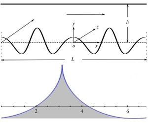
The purpose of the current work is to study analytically the effect of arbitrarily shaped one-dimensional corrugation waveforms on the hydraulic permeability (or the effective conductance) of channels with sizes that are neither large enough to be accessible for treatment as a shear flow, nor small enough to be accessible for treatment through lubrication approximation. The effect of inertia will be assumed to be vanishingly small, as typical in microfluidic applications. The method of domain perturbations (Van Dyke Reference Van Dyke1987; Hinch Reference Hinch1991), which involves the assumption of small characteristic amplitude to wavelength ratio and the shifting of boundary conditions to a convenient reference plane, will be employed. Finite-element simulations fully resolving the Stokes flow field are used for assessment of the analytical predictions for two specific shapes of wall undulations differing in their degree of smoothness. To enable the evaluation of the permeability when flow is oblique to the patterns, permeability will be evaluated in both the principal directions, i.e. in longitudinal flow where the applied pressure differential (or shear) is aligned along the pattern, and in transverse flow, where the applied forces are aligned across the pattern. Several new and convenient analytical results will be derived and validated for numerical accuracy. A hitherto unreported universal relationship valid for any prescribed periodic surface profile in confined flow, along the lines of those already known for the effective slip of isolated surfaces with patterned hydrodynamic slippage (Asmolov & Vinogradova Reference Asmolov and Vinogradova2012), which enables easy evaluation of permeability in the second principal direction once the permeability in the first principal direction is known, will be derived.
Panel (a) shows longitudinal/transverse flow through a channel with an arbitrarily shaped pattern on the bottom wall and a flat top wall. The pattern wavelength and the mean height of the channel is $L$
and
$L$
and $h$
, respectively. Panel (b) shows local coordinate systems
$h$
, respectively. Panel (b) shows local coordinate systems $xoz$
and
$xoz$
and $x^{\prime }oz^{\prime }$
with the ordinates aligned with the stripes and at an angle
$x^{\prime }oz^{\prime }$
with the ordinates aligned with the stripes and at an angle $\unicode[STIX]{x1D6FD}$
to the stripes, respectively. The permeabilities along and across the pattern direction are
$\unicode[STIX]{x1D6FD}$
to the stripes, respectively. The permeabilities along and across the pattern direction are $K_{\Vert }$
and
$K_{\Vert }$
and $K_{\bot }$
, respectively.
$K_{\bot }$
, respectively.

In § 2 a canonical confined flow problem, which is to be solved with arbitrary wall topography shape and arbitrary height is defined. In § 3 the hydraulic permeability is evaluated in longitudinal and transverse flow. A relationship is derived in this section between the components of the diagonalized permeability tensor. Section 3 also discusses the adaptation of the theory to other boundary conditions and flow configurations arising in applications. Section 4 specializes the analysis to specific test topographies, assesses the numerical accuracy of the asymptotic predictions and also discusses two distinct applications of the theory in the currently active area of slippery lubricant infused patterned surfaces placed in a dynamic fluid environment. This section also performs an experimental comparison with data from a complex topography studied in the literature. Section 5 discusses the main conclusions from the current work.
2 Problem definition
Incompressible laminar flow of a Newtonian fluid of viscosity $\unicode[STIX]{x1D707}$
and density
$\unicode[STIX]{x1D707}$
and density $\unicode[STIX]{x1D70C}$
is considered. The periodic cell of the channel through which the flow occurs is shown in figure 1(a). The lower wall is patterned topographically and can be located by the function
$\unicode[STIX]{x1D70C}$
is considered. The periodic cell of the channel through which the flow occurs is shown in figure 1(a). The lower wall is patterned topographically and can be located by the function $y=eg(x)$
, where
$y=eg(x)$
, where $e$
is a characteristic amplitude of the
$e$
is a characteristic amplitude of the $L$
-periodic pattern specified by the function
$L$
-periodic pattern specified by the function $g(x)$
. The channel has a flat wall at
$g(x)$
. The channel has a flat wall at $y=h$
. No-slip boundary condition is considered to apply on both the walls. The reference plane (
$y=h$
. No-slip boundary condition is considered to apply on both the walls. The reference plane ( $y=0$
) from which the ordinate
$y=0$
) from which the ordinate $g(x)$
is measured is chosen to be the ‘mean line’, to borrow a nomenclature from surface metrology (Whitehouse Reference Whitehouse1994). By this definition,
$g(x)$
is measured is chosen to be the ‘mean line’, to borrow a nomenclature from surface metrology (Whitehouse Reference Whitehouse1994). By this definition, $g(x)$
has to satisfy
$g(x)$
has to satisfy $\int _{-L/2}^{L/2}g(x)\,\text{d}x=0$
. The nominal thickness of the channel measured from the mean line is denoted by
$\int _{-L/2}^{L/2}g(x)\,\text{d}x=0$
. The nominal thickness of the channel measured from the mean line is denoted by $h$
. The flow is considered to be driven by a pressure drop
$h$
. The flow is considered to be driven by a pressure drop $\unicode[STIX]{x0394}P$
although extensions to shear-driven flow are discussed in and onward from § 3.4. The velocity components along the rectangular Cartesian coordinates
$\unicode[STIX]{x0394}P$
although extensions to shear-driven flow are discussed in and onward from § 3.4. The velocity components along the rectangular Cartesian coordinates $x,y,z$
(figure 1
a) are denoted by
$x,y,z$
(figure 1
a) are denoted by $u,v,w$
and the pressure is denoted by
$u,v,w$
and the pressure is denoted by $p$
.
$p$
.
A channel configuration with an unpatterned wall opposing a patterned wall, as shown in figure 1(a), is often preferred in microfluidic experiments from considerations such as ease of alignment (Feuillebois et al.
Reference Feuillebois, Bazant and Vinogradova2009) and/or optical access (Devasenathipathy, Santiago & Takehara Reference Devasenathipathy, Santiago and Takehara2002). While details of the analysis are demonstrated through the configuration in figure 1(a), several other confined flow configurations are studied later in § 3.4. It can be noted here that the geometry of figure 1(a) is also used by Stroock et al. (Reference Stroock, Dertinger, Whitesides and Ajdari2002) with a cosine shaped topography ( $g(x)=\cos (x)$
). Our subsequent findings would reduce to those of Stroock et al. (Reference Stroock, Dertinger, Whitesides and Ajdari2002) as special cases, providing partial validation of our results.
$g(x)=\cos (x)$
). Our subsequent findings would reduce to those of Stroock et al. (Reference Stroock, Dertinger, Whitesides and Ajdari2002) as special cases, providing partial validation of our results.
In the following, the inertia of the fluid will be neglected so that the flow is governed by the Stokes equations, as appropriate for microfluidic applications where the Reynolds number based on the characteristic size of the channel is small (Stone, Stroock & Ajdari Reference Stone, Stroock and Ajdari2004). There are also situations where physical and/or scaling arguments can justify the neglect of inertia in spite of a finite value of the Reynolds number based on the nominal channel height. These include unidirectional flow situations, e.g. when the periodic cell of figure 1(a) is located sufficiently far from entrances/exits and other disturbances to the flow, with the flow being directed parallel to the corrugations (longitudinal flow), as in § 3.1. Inertial effects can also be neglected on scaling grounds in the limiting situation of the channel size being an infinitesimal fraction of the patterning wavelength (Van Dyke Reference Van Dyke1987). Interestingly, the flow within the viscous sublayer of a turbulent external flow has been modelled as a zero-inertia flow by Bechert & Bartenwerfer (Reference Bechert and Bartenwerfer1989) and Luchini et al. (Reference Luchini, Manzo and Pozzi1991).
The following dimensionless variables are introduced for use in the rest of the article: $x=(L/2\unicode[STIX]{x03C0})X$
,
$x=(L/2\unicode[STIX]{x03C0})X$
, $y=(L/2\unicode[STIX]{x03C0})Y$
,
$y=(L/2\unicode[STIX]{x03C0})Y$
, $u=(U_{s})U$
,
$u=(U_{s})U$
, $v=(U_{s})V$
,
$v=(U_{s})V$
, $w=(U_{s})W$
,
$w=(U_{s})W$
, $p=(\unicode[STIX]{x0394}p/2\unicode[STIX]{x03C0})P$
, where the velocity scale
$p=(\unicode[STIX]{x0394}p/2\unicode[STIX]{x03C0})P$
, where the velocity scale $U_{s}$
will be specified shortly. The symbol
$U_{s}$
will be specified shortly. The symbol $\unicode[STIX]{x1D735}$
will signify the dimensionless gradient operator in the plane (
$\unicode[STIX]{x1D735}$
will signify the dimensionless gradient operator in the plane ( $x{-}y$
) of the topographic pattern. Incidentally, following the above non-dimensionalization scheme, the ratio of the inertia to viscous terms in the full Navier–Stokes equation would scale as
$x{-}y$
) of the topographic pattern. Incidentally, following the above non-dimensionalization scheme, the ratio of the inertia to viscous terms in the full Navier–Stokes equation would scale as $Re/H$
, where
$Re/H$
, where $Re=\unicode[STIX]{x1D70C}U_{s}h/\unicode[STIX]{x1D707}$
. The neglect of inertia will either require a strict Stokes flow assumption, or that
$Re=\unicode[STIX]{x1D70C}U_{s}h/\unicode[STIX]{x1D707}$
. The neglect of inertia will either require a strict Stokes flow assumption, or that $1/H$
be vanishingly small in the case
$1/H$
be vanishingly small in the case $Re\sim O(1)$
(or higher). Finite (but possibly large)
$Re\sim O(1)$
(or higher). Finite (but possibly large) $H$
is an important concern in what follows and the
$H$
is an important concern in what follows and the $O(1/H)$
terms retained in the finite-
$O(1/H)$
terms retained in the finite- $H$
analysis are not of inertial origin. Therefore, the finite-
$H$
analysis are not of inertial origin. Therefore, the finite- $H$
analysis applies only to Stokes flow and additional corrections stemming from the inertia terms would be needed for a flow where
$H$
analysis applies only to Stokes flow and additional corrections stemming from the inertia terms would be needed for a flow where $Re\sim O(1)$
or higher. The shear-based scale
$Re\sim O(1)$
or higher. The shear-based scale $U_{s}=\unicode[STIX]{x0394}ph/2\unicode[STIX]{x03C0}\unicode[STIX]{x1D707}$
for velocity is used in the remainder of the articlehere. This scale is crucial for understanding the effect of finite channel size studied later in the article.
$U_{s}=\unicode[STIX]{x0394}ph/2\unicode[STIX]{x03C0}\unicode[STIX]{x1D707}$
for velocity is used in the remainder of the articlehere. This scale is crucial for understanding the effect of finite channel size studied later in the article.
The concern of this article is to obtain reliable analytical (preferably closed-form) estimates of the channel hydraulic permeability in Stokes flow, in the presence of arbitrary wall patterns. The permeability ( $k$
) is defined as the volumetric flow rate of a fluid of unit viscosity in a channel subject to unit pressure gradient, and has dimensions of length squared. However, in most of the subsequent development,
$k$
) is defined as the volumetric flow rate of a fluid of unit viscosity in a channel subject to unit pressure gradient, and has dimensions of length squared. However, in most of the subsequent development, $k$
will be normalized by the permeability of the corresponding channel of height
$k$
will be normalized by the permeability of the corresponding channel of height $h$
where the wall patterns are absent (
$h$
where the wall patterns are absent ( $e=0$
), leading to the dimensionless permeability
$e=0$
), leading to the dimensionless permeability $K$
. The symbol for permeability may be superscripted/subscripted where necessary to indicate flow, channel and pattern types. It may be noted that the dimensionless permeability can also be interpreted as the ratio of the Poiseuille number of the unpatterned channel to that of the patterned channel. The Poiseuille number is proportional to the product of the Fanning/Darcy friction factor and the Reynolds number (Taylor Reference Taylor1971).
$K$
. The symbol for permeability may be superscripted/subscripted where necessary to indicate flow, channel and pattern types. It may be noted that the dimensionless permeability can also be interpreted as the ratio of the Poiseuille number of the unpatterned channel to that of the patterned channel. The Poiseuille number is proportional to the product of the Fanning/Darcy friction factor and the Reynolds number (Taylor Reference Taylor1971).
If the flow direction is oblique to stripes (figure 1
b), the resultant tensorial permeability (Bazant & Vinogradova Reference Bazant and Vinogradova2008; Schmieschek et al.
Reference Schmieschek, Belyaev, Harting and Vinogradova2012) is completely determined by the permeability in the two canonical directions ( $z$
and
$z$
and $x$
) along and across the stripes, which are termed longitudinal and transverse flow, respectively. Further details on the tensorial nature of permeability relevant to the current study are discussed in the beginning of the next section.
$x$
) along and across the stripes, which are termed longitudinal and transverse flow, respectively. Further details on the tensorial nature of permeability relevant to the current study are discussed in the beginning of the next section.
3 The hydraulic permeability tensor
In an infinite Hele-Shaw cell with one-dimensional wall topography, the direction of net fluid permeation is, in general, different from the direction of applied forces (Ajdari Reference Ajdari2001; Ghosal Reference Ghosal2002). Let the vector $\boldsymbol{K}_{\unicode[STIX]{x1D6FD}}$
encode the magnitude of the normalized hydraulic permeability and the direction of fluid permeation. Referring to figure 1(b), the components of
$\boldsymbol{K}_{\unicode[STIX]{x1D6FD}}$
encode the magnitude of the normalized hydraulic permeability and the direction of fluid permeation. Referring to figure 1(b), the components of $\boldsymbol{K}_{\unicode[STIX]{x1D6FD}}$
along and perpendicular to any direction
$\boldsymbol{K}_{\unicode[STIX]{x1D6FD}}$
along and perpendicular to any direction $\overrightarrow{OX^{\prime }}$
oriented at an angle
$\overrightarrow{OX^{\prime }}$
oriented at an angle $\unicode[STIX]{x1D6FD}$
with respect to the one-dimensional striped pattern can be calculated using the relation
$\unicode[STIX]{x1D6FD}$
with respect to the one-dimensional striped pattern can be calculated using the relation $\boldsymbol{K}_{\unicode[STIX]{x1D6FD}}=\unicode[STIX]{x1D648}\hat{l}$
, where
$\boldsymbol{K}_{\unicode[STIX]{x1D6FD}}=\unicode[STIX]{x1D648}\hat{l}$
, where $\hat{l}=(l^{\prime },m^{\prime })$
are the direction cosines of the applied force causing the fluid flux in the
$\hat{l}=(l^{\prime },m^{\prime })$
are the direction cosines of the applied force causing the fluid flux in the $x^{\prime }-z^{\prime }$
coordinate system. The tensor
$x^{\prime }-z^{\prime }$
coordinate system. The tensor $\unicode[STIX]{x1D648}$
is given by
$\unicode[STIX]{x1D648}$
is given by $\unicode[STIX]{x1D648}=R_{-\unicode[STIX]{x1D6FD}}\,\text{diag}(K_{\Vert },K_{\bot })R_{\unicode[STIX]{x1D6FD}}$
(Ajdari Reference Ajdari2001; Bazant & Vinogradova Reference Bazant and Vinogradova2008; Feuillebois et al.
Reference Feuillebois, Bazant and Vinogradova2010) and will be termed the hydraulic permeability tensor here. Here,
$\unicode[STIX]{x1D648}=R_{-\unicode[STIX]{x1D6FD}}\,\text{diag}(K_{\Vert },K_{\bot })R_{\unicode[STIX]{x1D6FD}}$
(Ajdari Reference Ajdari2001; Bazant & Vinogradova Reference Bazant and Vinogradova2008; Feuillebois et al.
Reference Feuillebois, Bazant and Vinogradova2010) and will be termed the hydraulic permeability tensor here. Here, $R_{\unicode[STIX]{x1D6FD}}$
is the two-dimensional matrix that rotates points in the (
$R_{\unicode[STIX]{x1D6FD}}$
is the two-dimensional matrix that rotates points in the ( $x{-}z$
) plane by an angle
$x{-}z$
) plane by an angle $\unicode[STIX]{x1D6FD}$
. Since the only non-geometrical parameters affecting
$\unicode[STIX]{x1D6FD}$
. Since the only non-geometrical parameters affecting $\unicode[STIX]{x1D648}$
are
$\unicode[STIX]{x1D648}$
are $K_{\Vert }$
and
$K_{\Vert }$
and $K_{\bot }$
, the rest of the theoretical development is devoted to evaluating
$K_{\bot }$
, the rest of the theoretical development is devoted to evaluating $K_{||}$
for longitudinal flow (§ 3.1) and
$K_{||}$
for longitudinal flow (§ 3.1) and $K_{\bot }$
for transverse flow (§ 3.2) by solving the respective flow problems.
$K_{\bot }$
for transverse flow (§ 3.2) by solving the respective flow problems.
3.1 Longitudinal flow
With respect to the longitudinal flow through the geometry shown in figure 1(a), the velocity $W(X,Y)$
of the unidirectional flow is governed by the balance of viscous and pressure forces while the no-slip boundary conditions apply at both the corrugated bottom wall and the flat top wall, leading to
$W(X,Y)$
of the unidirectional flow is governed by the balance of viscous and pressure forces while the no-slip boundary conditions apply at both the corrugated bottom wall and the flat top wall, leading to
 $$\begin{eqnarray}\displaystyle & \displaystyle \unicode[STIX]{x1D6FB}^{2}W=-\frac{1}{H}, & \displaystyle\end{eqnarray}$$
 $$\begin{eqnarray}\displaystyle & \displaystyle W(X,\unicode[STIX]{x1D716}g(X))=0, & \displaystyle\end{eqnarray}$$
 $$\begin{eqnarray}\displaystyle & \displaystyle W(X,H)=0. & \displaystyle\end{eqnarray}$$ $\unicode[STIX]{x1D716}=2\unicode[STIX]{x03C0}e/L$
and
$\unicode[STIX]{x1D716}=2\unicode[STIX]{x03C0}e/L$
and $H=2\unicode[STIX]{x03C0}h/L$
are a characteristic pattern size and the nominal channel thickness, rendered dimensionless through multiplication with the pattern wavenumber
$H=2\unicode[STIX]{x03C0}h/L$
are a characteristic pattern size and the nominal channel thickness, rendered dimensionless through multiplication with the pattern wavenumber $2\unicode[STIX]{x03C0}/L$
. The
$2\unicode[STIX]{x03C0}/L$
. The $H$
-dependent right-hand side of (3.1a
) is a consequence of the wall-shear-based velocity scale
$H$
-dependent right-hand side of (3.1a
) is a consequence of the wall-shear-based velocity scale $(\unicode[STIX]{x0394}ph/2\unicode[STIX]{x03C0}\unicode[STIX]{x1D707})$
.
$(\unicode[STIX]{x0394}ph/2\unicode[STIX]{x03C0}\unicode[STIX]{x1D707})$
.
In the following, $\unicode[STIX]{x1D716}$
will be treated as a small parameter, and asymptotic expansions in the form
$\unicode[STIX]{x1D716}$
will be treated as a small parameter, and asymptotic expansions in the form $W=W^{0}+\unicode[STIX]{x1D716}W^{1}+\unicode[STIX]{x1D716}^{2}W^{2}+o(\unicode[STIX]{x1D716}^{2})$
together with the method of domain perturbations (Hinch Reference Hinch1991), which involves the transfer the boundary condition on the curved surface (3.1b
) to
$W=W^{0}+\unicode[STIX]{x1D716}W^{1}+\unicode[STIX]{x1D716}^{2}W^{2}+o(\unicode[STIX]{x1D716}^{2})$
together with the method of domain perturbations (Hinch Reference Hinch1991), which involves the transfer the boundary condition on the curved surface (3.1b
) to $Y=0$
through the Taylor expansion
$Y=0$
through the Taylor expansion $W(X,\unicode[STIX]{x1D716}g(X))=W(X,0)+\unicode[STIX]{x1D716}gW_{Y}(X,0)+\unicode[STIX]{x1D716}^{2}g^{2}W_{YY}(X,0)/2+o(\unicode[STIX]{x1D716}^{2})$
, will be employed. Here, subscripts denote derivative. Since the highest-order correction evaluated in this study is
$W(X,\unicode[STIX]{x1D716}g(X))=W(X,0)+\unicode[STIX]{x1D716}gW_{Y}(X,0)+\unicode[STIX]{x1D716}^{2}g^{2}W_{YY}(X,0)/2+o(\unicode[STIX]{x1D716}^{2})$
, will be employed. Here, subscripts denote derivative. Since the highest-order correction evaluated in this study is $W^{2}$
, algebraic expressions for the normalized permeability derived in §§ 3, 3.4 and 4 will contain an
$W^{2}$
, algebraic expressions for the normalized permeability derived in §§ 3, 3.4 and 4 will contain an $o(\unicode[STIX]{x1D716}^{2})$
error term, even though the same will be indicated explicitly only when important to the discussion. The ‘little o’ asymptotic notation used here may be noted.
$o(\unicode[STIX]{x1D716}^{2})$
error term, even though the same will be indicated explicitly only when important to the discussion. The ‘little o’ asymptotic notation used here may be noted.
3.1.1 Leading order ( $O(1)$
)
$O(1)$
)

The leading-order solution is obtained by setting $\unicode[STIX]{x1D716}=0$
and corresponds to a flat bottom wall at
$\unicode[STIX]{x1D716}=0$
and corresponds to a flat bottom wall at $Y=0$
, where the
$Y=0$
, where the $X$
independent flow velocity
$X$
independent flow velocity $W^{0}$
is given by
$W^{0}$
is given by
 $$\begin{eqnarray}W^{0}=\frac{Y}{2}-\frac{Y^{2}}{2H}.\end{eqnarray}$$
3.1.2 The
$O(\unicode[STIX]{x1D716})$
correction

The governing equation and no-slip boundary conditions for $W^{1}$
are
$W^{1}$
are
 $$\begin{eqnarray}\displaystyle & \displaystyle \unicode[STIX]{x1D6FB}^{2}W^{1}=0, & \displaystyle\end{eqnarray}$$
 $$\begin{eqnarray}\displaystyle & \displaystyle W^{1}(X,0)+g(X)W_{Y}^{0}(X,0)=0, & \displaystyle\end{eqnarray}$$
 $$\begin{eqnarray}\displaystyle & \displaystyle W^{1}(X,H)=0, & \displaystyle\end{eqnarray}$$
 $$\begin{eqnarray}\displaystyle & \displaystyle W^{1}(X,Y)=\mathop{\sum }_{n\neq 0}^{\infty }C_{1n}(\text{e}^{-|n|Y}-\text{e}^{-2|n|H}\text{e}^{|n|Y})\text{e}^{\text{i}nX}, & \displaystyle\end{eqnarray}$$
 $$\begin{eqnarray}\displaystyle & \displaystyle C_{1n}=-\frac{g_{n}}{2(1-\text{e}^{-2|n|H})}. & \displaystyle\end{eqnarray}$$ $n\neq 0$
denotes a sum taken through all integers except zero.
$n\neq 0$
denotes a sum taken through all integers except zero.
3.1.3 The
$O(\unicode[STIX]{x1D716}^{2})$
correction

The governing equation and no-slip boundary conditions for $W^{2}$
are
$W^{2}$
are
 $$\begin{eqnarray}\displaystyle & \displaystyle \unicode[STIX]{x1D6FB}^{2}W^{2}=0, & \displaystyle\end{eqnarray}$$
 $$\begin{eqnarray}\displaystyle & \displaystyle W^{2}(X,0)+g(X)W_{Y}^{1}(X,0)+\frac{g(X)^{2}}{2}W_{YY}^{0}(X,0)=0, & \displaystyle\end{eqnarray}$$
 $$\begin{eqnarray}\displaystyle & \displaystyle W^{2}(X,H)=0, & \displaystyle\end{eqnarray}$$ $O(\unicode[STIX]{x1D716}^{2})$
-accurate prediction of the permeability, to find an expression for the period-averaged velocity
$O(\unicode[STIX]{x1D716}^{2})$
-accurate prediction of the permeability, to find an expression for the period-averaged velocity $\langle W^{2}(X,Y)\rangle$
, which is the part of
$\langle W^{2}(X,Y)\rangle$
, which is the part of $W_{2}$
obtained by excluding its harmonic (
$W_{2}$
obtained by excluding its harmonic ( $\propto \text{e}^{\text{i}nX},n\neq 0$
) parts. The quantity
$\propto \text{e}^{\text{i}nX},n\neq 0$
) parts. The quantity $\langle W^{2}(X,Y)\rangle$
is given by
$\langle W^{2}(X,Y)\rangle$
is given by  $$\begin{eqnarray}\displaystyle & \displaystyle \langle W^{2}(X,Y)\rangle =C^{\Vert }\left(1-\frac{Y}{H}\right), & \displaystyle\end{eqnarray}$$
 $$\begin{eqnarray}\displaystyle & \displaystyle C^{\Vert }=-S_{1}^{\Vert }+\frac{S_{2}}{H}, & \displaystyle\end{eqnarray}$$
 $$\begin{eqnarray}\displaystyle & \displaystyle S_{1}^{\Vert }=\mathop{\sum }_{n=1}^{\infty }n\coth (nH){|g_{n}|}^{2}, & \displaystyle\end{eqnarray}$$
 $$\begin{eqnarray}\displaystyle & \displaystyle S_{2}=\mathop{\sum }_{n=1}^{\infty }{|g_{n}|}^{2}. & \displaystyle\end{eqnarray}$$ $S_{1}^{\Vert }$
arises from convolution of the Fourier series of
$S_{1}^{\Vert }$
arises from convolution of the Fourier series of $g$
into that of its
$g$
into that of its $y$
derivative and for a given surface topography, its convergence is crucial to obtaining meaningful answers from the domain perturbation method. The series
$y$
derivative and for a given surface topography, its convergence is crucial to obtaining meaningful answers from the domain perturbation method. The series $S_{2}$
converges to
$S_{2}$
converges to $1/4\unicode[STIX]{x03C0}$
times the variance of the topography, as per Parseval’s identity.
$1/4\unicode[STIX]{x03C0}$
times the variance of the topography, as per Parseval’s identity.
3.1.4 Effective permeability
The effective dimensionless permeability $K$
is obtained from the dimensionless flow rate
$K$
is obtained from the dimensionless flow rate $Q(\unicode[STIX]{x1D716},H)$
using its definition discussed in § 2, which leads to
$Q(\unicode[STIX]{x1D716},H)$
using its definition discussed in § 2, which leads to $K=Q(\unicode[STIX]{x1D716},H)/Q(0,H)$
. Here, the functional argument of
$K=Q(\unicode[STIX]{x1D716},H)/Q(0,H)$
. Here, the functional argument of $Q$
within parentheses indicate the dependence of
$Q$
within parentheses indicate the dependence of $Q$
on
$Q$
on $\unicode[STIX]{x1D716}$
and
$\unicode[STIX]{x1D716}$
and $H$
. In longitudinal flow,
$H$
. In longitudinal flow, $Q$
is obtained from an
$Q$
is obtained from an $O(\unicode[STIX]{x1D716}^{2})$
-accurate Taylor-series approximation of
$O(\unicode[STIX]{x1D716}^{2})$
-accurate Taylor-series approximation of
 $$\begin{eqnarray}Q^{\Vert }(\unicode[STIX]{x1D716},H)=\int _{-\unicode[STIX]{x03C0}}^{\unicode[STIX]{x03C0}}\int _{\unicode[STIX]{x1D716}g(X)}^{H}W\,\text{d}Y\,\text{d}X=\int _{-\unicode[STIX]{x03C0}}^{\unicode[STIX]{x03C0}}\int _{\unicode[STIX]{x1D716}g(X)}^{H}[W^{0}+\unicode[STIX]{x1D716}W^{1}+\unicode[STIX]{x1D716}^{2}\langle W^{2}\rangle +o(\unicode[STIX]{x1D716}^{2})]\,\text{d}Y\,\text{d}X.\end{eqnarray}$$
As discussed below equation (3.5), the harmonic parts of $W_{2}$
do not contribute to the
$W_{2}$
do not contribute to the $O(\unicode[STIX]{x1D716}^{2})$
-accurate flow rate.
$O(\unicode[STIX]{x1D716}^{2})$
-accurate flow rate.
Below, we first provide expressions for $K$
which are applicable to arbitrary channel height. Then, at the cost of errors that decay exponentially fast with
$K$
which are applicable to arbitrary channel height. Then, at the cost of errors that decay exponentially fast with $H$
, we derive expressions for large but finite channel height that are simpler and often more tractable in closed form. Below, a ‘relative roughness’ parameter
$H$
, we derive expressions for large but finite channel height that are simpler and often more tractable in closed form. Below, a ‘relative roughness’ parameter $\unicode[STIX]{x1D6FC}=e/h=\unicode[STIX]{x1D716}/H$
is introduced in the expressions for
$\unicode[STIX]{x1D6FC}=e/h=\unicode[STIX]{x1D716}/H$
is introduced in the expressions for $K$
in favour of
$K$
in favour of $\unicode[STIX]{x1D716}$
as one of the independent variables, borrowing familiar terminology from the celebrated Moody chart for the Darcy–Weisbach friction factor (Taylor Reference Taylor1971) and notation from the study on sinusoidal patterns by Stroock et al. (Reference Stroock, Dertinger, Whitesides and Ajdari2002).
$\unicode[STIX]{x1D716}$
as one of the independent variables, borrowing familiar terminology from the celebrated Moody chart for the Darcy–Weisbach friction factor (Taylor Reference Taylor1971) and notation from the study on sinusoidal patterns by Stroock et al. (Reference Stroock, Dertinger, Whitesides and Ajdari2002).
For arbitrary channel height. The following expressions for the normalized permeability are obtained on integrating $W$
using (3.7) to
$W$
using (3.7) to $O(\unicode[STIX]{x1D716}^{2})$
accuracy:
$O(\unicode[STIX]{x1D716}^{2})$
accuracy:
 $$\begin{eqnarray}K_{\Vert }=1-6\unicode[STIX]{x1D6FC}^{2}(HS_{1}^{\Vert }-S_{2})+o(\unicode[STIX]{x1D716}^{2}).\end{eqnarray}$$
For the special case of $g(x)=\cos (x)$
, equation (3.8) reduces to a scaled version of (13) from Stroock et al. (Reference Stroock, Dertinger, Whitesides and Ajdari2002), reassuring our
$g(x)=\cos (x)$
, equation (3.8) reduces to a scaled version of (13) from Stroock et al. (Reference Stroock, Dertinger, Whitesides and Ajdari2002), reassuring our $H$
-dependent calculations.
$H$
-dependent calculations.
Exponentially accurate approximation of the effect of finite channel height. The nominally ‘large $H$
’ approximation to be discussed now is one of the important contributions of the current study. It amounts to setting to zero all terms that signify integral powers of
$H$
’ approximation to be discussed now is one of the important contributions of the current study. It amounts to setting to zero all terms that signify integral powers of $\text{e}^{-H}$
in the preceding expressions, without altering any terms that decay algebraically with
$\text{e}^{-H}$
in the preceding expressions, without altering any terms that decay algebraically with $H$
, i.e. the terms containing integral powers of
$H$
, i.e. the terms containing integral powers of $1/H$
. The important consequences from this limiting process are
$1/H$
. The important consequences from this limiting process are
 $$\begin{eqnarray}\displaystyle & \displaystyle W^{1}(X,Y)=\frac{1}{2}\mathop{\sum }_{n\neq 0}^{\infty }g_{n}\text{e}^{-|n|Y}\text{e}^{\text{i}nX}+e.s.t.(H), & \displaystyle\end{eqnarray}$$
 $$\begin{eqnarray}\displaystyle & \displaystyle C^{\Vert }=-S_{1}+\frac{S_{2}}{H}+e.s.t.(H)=-S_{1}+O(1/H), & \displaystyle\end{eqnarray}$$
 $$\begin{eqnarray}\displaystyle & \displaystyle S_{1}=\mathop{\sum }_{n=1}^{\infty }n{|g_{n}|}^{2} & \displaystyle\end{eqnarray}$$ $W^{2}$
still continues to be given by (3.6).
$W^{2}$
still continues to be given by (3.6).
In (3.9) and the remainder of the article, the abbreviation $e.s.t.(H)$
signifies terms that decrease exponentially fast with increase of
$e.s.t.(H)$
signifies terms that decrease exponentially fast with increase of $H$
, i.e. ‘exponentially small terms’ at large
$H$
, i.e. ‘exponentially small terms’ at large $H$
. The
$H$
. The $e.s.t.(H)$
always arise in the contribution from non-zero wavenumbers in the dependent variables, i.e. in their harmonic (
$e.s.t.(H)$
always arise in the contribution from non-zero wavenumbers in the dependent variables, i.e. in their harmonic ( $n\neq 0$
) parts. The convergence of the sum
$n\neq 0$
) parts. The convergence of the sum $S_{1}$
is crucial to the meaningfulness of large
$S_{1}$
is crucial to the meaningfulness of large $H$
predictions.
$H$
predictions.
The first equality of (3.9b
) pertains to the large- $H$
approximation promulgated in the current work. The intuitively ‘cruder’ algebraically accurate estimate of
$H$
approximation promulgated in the current work. The intuitively ‘cruder’ algebraically accurate estimate of $C^{\Vert }$
given by the second equality of (3.9b
) will also be discussed shortly and later subject to numerical evaluations.
$C^{\Vert }$
given by the second equality of (3.9b
) will also be discussed shortly and later subject to numerical evaluations.
In terms of the steps followed in §§ 3.1.1–3.1.3, the neglect of $e.s.t.(H)$
terms in the manner discussed above leaves the governing equations and the patterned wall boundary condition unaffected. Also,
$e.s.t.(H)$
terms in the manner discussed above leaves the governing equations and the patterned wall boundary condition unaffected. Also, $\langle W^{0}\rangle =W^{0}$
,
$\langle W^{0}\rangle =W^{0}$
, $\langle W^{1}\rangle =0$
and
$\langle W^{1}\rangle =0$
and $\langle W^{2}\rangle$
remain compliant to the boundary condition of
$\langle W^{2}\rangle$
remain compliant to the boundary condition of $Y=H$
(here no slip). However, errors that decrease exponentially fast with increase of
$Y=H$
(here no slip). However, errors that decrease exponentially fast with increase of $H$
are incurred at
$H$
are incurred at $Y=H$
for the harmonic (
$Y=H$
for the harmonic ( $n\neq 0$
) parts of the functions
$n\neq 0$
) parts of the functions $W^{1}$
and
$W^{1}$
and $W^{2}$
. It may also be worthwhile to recall here that imposition of boundary conditions on a non-planar boundary such as
$W^{2}$
. It may also be worthwhile to recall here that imposition of boundary conditions on a non-planar boundary such as $Y=\unicode[STIX]{x1D716}g(X)$
by any domain perturbation method is only algebraically accurate in
$Y=\unicode[STIX]{x1D716}g(X)$
by any domain perturbation method is only algebraically accurate in $\unicode[STIX]{x1D716}$
(Van Dyke Reference Van Dyke1987).
$\unicode[STIX]{x1D716}$
(Van Dyke Reference Van Dyke1987).
Interestingly, another equivalent, algebraically less cumbersome way of deriving the large- $H$
solution can be perceived. In this method, the exact imposition of the top wall boundary condition can be avoided from the onset of the analysis, except for zero wavenumber terms at each order. Thus, an effective far-field condition can instead be specified (with certain constants for the yet-to-be-determined far field), as follows:
$H$
solution can be perceived. In this method, the exact imposition of the top wall boundary condition can be avoided from the onset of the analysis, except for zero wavenumber terms at each order. Thus, an effective far-field condition can instead be specified (with certain constants for the yet-to-be-determined far field), as follows:
 $$\begin{eqnarray}\text{As }y\rightarrow \infty ,\quad W\rightarrow \frac{Y}{2}-\frac{Y^{2}}{2H}+(\unicode[STIX]{x1D716}\tilde{C}^{\Vert }+\unicode[STIX]{x1D716}^{2}C^{\Vert })\left(1-\frac{Y}{H}\right).\end{eqnarray}$$
Equation (3.10) can also be interpreted as a carefully chosen superposition of linear and quadratic shear flows. On further analysis, the constant $\tilde{C}^{\Vert }$
in (3.10) can be evaluated to be zero due to the boundary condition on the patterned wall and the choice of the origin on the mean line, whereas the constant
$\tilde{C}^{\Vert }$
in (3.10) can be evaluated to be zero due to the boundary condition on the patterned wall and the choice of the origin on the mean line, whereas the constant $C^{\Vert }$
comes out as given in (3.9b
). In contrast to the overall presentation of the current section, the authors could infer the large-
$C^{\Vert }$
comes out as given in (3.9b
). In contrast to the overall presentation of the current section, the authors could infer the large- $H$
relations, before formally deriving the finite-
$H$
relations, before formally deriving the finite- $H$
relations using the method outlined above. To infer the pattern-averaged streamwise velocity field
$H$
relations using the method outlined above. To infer the pattern-averaged streamwise velocity field $\langle W\rangle$
in the large-
$\langle W\rangle$
in the large- $H$
regime, the adjusted effective slip length
$H$
regime, the adjusted effective slip length $L_{eff}-\unicode[STIX]{x1D716}^{2}/HS_{2}$
can be used, where
$L_{eff}-\unicode[STIX]{x1D716}^{2}/HS_{2}$
can be used, where $L_{eff}$
is the effective slip length for the corresponding unbounded (infinite-
$L_{eff}$
is the effective slip length for the corresponding unbounded (infinite- $H$
) shear flow. The adjustment
$H$
) shear flow. The adjustment $-\unicode[STIX]{x1D716}^{2}S_{2}/H$
is a consequence of the curvature of the
$-\unicode[STIX]{x1D716}^{2}S_{2}/H$
is a consequence of the curvature of the $\langle W\rangle$
field (
$\langle W\rangle$
field ( $\langle W\rangle _{YY}=W_{0YY}\neq 0$
unlike shear flow) and arises from the application of Parseval’s identity to the last term on the left-hand side equation (3.5b
).
$\langle W\rangle _{YY}=W_{0YY}\neq 0$
unlike shear flow) and arises from the application of Parseval’s identity to the last term on the left-hand side equation (3.5b
).
On evaluating the flow rate, the final large- $H$
permeability estimate is obtained from
$H$
permeability estimate is obtained from
 $$\begin{eqnarray}\tilde{K}_{\Vert }=(1-6\unicode[STIX]{x1D6FC}^{2}HS_{1})+12\unicode[STIX]{x1D6FC}^{2}S_{2}+e.s.t.(H)+o(\unicode[STIX]{x1D716}^{2}).\end{eqnarray}$$
Here and henceforth in the article, the superscript ${\sim}$
is used to signify the exponentially accurate approximation of the finite channel height effect. The term enclosed by brackets in (3.11) signifies an estimate of permeability based on the expression to the right of the second equality in (3.9b
), which amounts to also neglecting terms of
${\sim}$
is used to signify the exponentially accurate approximation of the finite channel height effect. The term enclosed by brackets in (3.11) signifies an estimate of permeability based on the expression to the right of the second equality in (3.9b
), which amounts to also neglecting terms of $C_{\Vert }$
that are algebraically decaying in
$C_{\Vert }$
that are algebraically decaying in $H$
. Incidentally, and as discussed later in the article, the expression to the right of the second equality (without the term under the order symbol) in (3.9b
) also signifies half the effective slip length of the patterned surface in shear flow (Luchini et al.
Reference Luchini, Manzo and Pozzi1991).
$H$
. Incidentally, and as discussed later in the article, the expression to the right of the second equality (without the term under the order symbol) in (3.9b
) also signifies half the effective slip length of the patterned surface in shear flow (Luchini et al.
Reference Luchini, Manzo and Pozzi1991).
3.2 Transverse flow
The transverse flow is solved conveniently in terms of the streamfunction $\unicode[STIX]{x1D713}$
defined through
$\unicode[STIX]{x1D713}$
defined through $U=\unicode[STIX]{x2202}\unicode[STIX]{x1D713}/\unicode[STIX]{x2202}Y$
and
$U=\unicode[STIX]{x2202}\unicode[STIX]{x1D713}/\unicode[STIX]{x2202}Y$
and $V=-\unicode[STIX]{x2202}\unicode[STIX]{x1D713}/\unicode[STIX]{x2202}X$
. For Stokes flow with a specified pressure drop between
$V=-\unicode[STIX]{x2202}\unicode[STIX]{x1D713}/\unicode[STIX]{x2202}X$
. For Stokes flow with a specified pressure drop between $X=-\unicode[STIX]{x03C0}$
and
$X=-\unicode[STIX]{x03C0}$
and $X=\unicode[STIX]{x03C0}$
in a channel subject to no slip and no penetration on both the corrugated and planar boundaries of figure 1(a), the following need to be observed:
$X=\unicode[STIX]{x03C0}$
in a channel subject to no slip and no penetration on both the corrugated and planar boundaries of figure 1(a), the following need to be observed:
 $$\begin{eqnarray}\displaystyle & \displaystyle \unicode[STIX]{x1D6FB}^{4}\unicode[STIX]{x1D713}=0, & \displaystyle\end{eqnarray}$$
 $$\begin{eqnarray}\displaystyle & \displaystyle \frac{\unicode[STIX]{x2202}^{3}\langle \unicode[STIX]{x1D713}\rangle }{\unicode[STIX]{x2202}Y^{3}}=-\frac{1}{H}, & \displaystyle\end{eqnarray}$$
 $$\begin{eqnarray}\displaystyle & \displaystyle \unicode[STIX]{x1D713}(X,\unicode[STIX]{x1D716}g(X))=0, & \displaystyle\end{eqnarray}$$
 $$\begin{eqnarray}\displaystyle & \displaystyle \unicode[STIX]{x1D713}_{Y}(X,\unicode[STIX]{x1D716}g(X))=0, & \displaystyle\end{eqnarray}$$
 $$\begin{eqnarray}\displaystyle & \displaystyle \unicode[STIX]{x1D713}_{X}(X,H)=0, & \displaystyle\end{eqnarray}$$
 $$\begin{eqnarray}\displaystyle & \displaystyle \unicode[STIX]{x1D713}_{Y}(X,H)=0. & \displaystyle\end{eqnarray}$$
In the following, $\unicode[STIX]{x1D716}=2\unicode[STIX]{x03C0}e/L$
will be treated as a small parameter, and the asymptotic expansions in the form
$\unicode[STIX]{x1D716}=2\unicode[STIX]{x03C0}e/L$
will be treated as a small parameter, and the asymptotic expansions in the form $\unicode[STIX]{x1D713}=\unicode[STIX]{x1D713}^{0}+\unicode[STIX]{x1D716}\unicode[STIX]{x1D713}^{1}+\unicode[STIX]{x1D716}^{2}\unicode[STIX]{x1D713}^{2}+o(\unicode[STIX]{x1D716}^{2})$
together with the method of domain perturbations (Hinch Reference Hinch1991), which involves the transfer the boundary conditions on the curved surface ((3.12c
) and (3.12d
)) to
$\unicode[STIX]{x1D713}=\unicode[STIX]{x1D713}^{0}+\unicode[STIX]{x1D716}\unicode[STIX]{x1D713}^{1}+\unicode[STIX]{x1D716}^{2}\unicode[STIX]{x1D713}^{2}+o(\unicode[STIX]{x1D716}^{2})$
together with the method of domain perturbations (Hinch Reference Hinch1991), which involves the transfer the boundary conditions on the curved surface ((3.12c
) and (3.12d
)) to $Y=0$
through the Taylor expansion
$Y=0$
through the Taylor expansion $\unicode[STIX]{x1D713}(X,\unicode[STIX]{x1D716}g(X))=\unicode[STIX]{x1D713}(X,0)+\unicode[STIX]{x1D716}g\unicode[STIX]{x1D713}_{Y}(X,0)+\unicode[STIX]{x1D716}^{2}g^{2}\unicode[STIX]{x1D713}_{YY}(X,0)/2+o(\unicode[STIX]{x1D716}^{2})$
and a similar expression for
$\unicode[STIX]{x1D713}(X,\unicode[STIX]{x1D716}g(X))=\unicode[STIX]{x1D713}(X,0)+\unicode[STIX]{x1D716}g\unicode[STIX]{x1D713}_{Y}(X,0)+\unicode[STIX]{x1D716}^{2}g^{2}\unicode[STIX]{x1D713}_{YY}(X,0)/2+o(\unicode[STIX]{x1D716}^{2})$
and a similar expression for $\unicode[STIX]{x1D713}_{Y}(X,\unicode[STIX]{x1D716}g(X))$
, will be employed. Here, subscripts denote a derivative. Since the highest-order correction evaluated in this study is
$\unicode[STIX]{x1D713}_{Y}(X,\unicode[STIX]{x1D716}g(X))$
, will be employed. Here, subscripts denote a derivative. Since the highest-order correction evaluated in this study is $\unicode[STIX]{x1D713}^{2}$
, all algebraic expressions derived in the current section will contain an
$\unicode[STIX]{x1D713}^{2}$
, all algebraic expressions derived in the current section will contain an $o(\unicode[STIX]{x1D716}^{2})$
error term. However, for conciseness, this error will not be indicated explicitly in the equations to follow, barring a few exceptions.
$o(\unicode[STIX]{x1D716}^{2})$
error term. However, for conciseness, this error will not be indicated explicitly in the equations to follow, barring a few exceptions.
3.2.1 Leading order (
$O(1)$
)

The leading-order solution is obtained by setting $\unicode[STIX]{x1D716}=0$
and corresponds to a flat bottom wall at
$\unicode[STIX]{x1D716}=0$
and corresponds to a flat bottom wall at $Y=0$
, where the
$Y=0$
, where the $X$
independent streamfunction
$X$
independent streamfunction $\unicode[STIX]{x1D713}^{0}$
is given by
$\unicode[STIX]{x1D713}^{0}$
is given by
 $$\begin{eqnarray}\unicode[STIX]{x1D713}^{0}=\frac{Y^{2}}{4}-\frac{Y^{3}}{6H}.\end{eqnarray}$$
3.2.2 The
$O(\unicode[STIX]{x1D716})$
correction

The first correction $\unicode[STIX]{x1D713}^{1}$
is governed by
$\unicode[STIX]{x1D713}^{1}$
is governed by
 $$\begin{eqnarray}\displaystyle & \displaystyle \unicode[STIX]{x1D6FB}^{4}\unicode[STIX]{x1D713}^{1}=0, & \displaystyle\end{eqnarray}$$
 $$\begin{eqnarray}\displaystyle & \displaystyle \frac{\unicode[STIX]{x2202}^{3}\langle \unicode[STIX]{x1D713}^{1}\rangle }{\unicode[STIX]{x2202}Y^{3}}=0, & \displaystyle\end{eqnarray}$$
 $$\begin{eqnarray}\displaystyle & \displaystyle \unicode[STIX]{x1D713}^{1}(X,0)+g(X)\unicode[STIX]{x1D713}_{Y}^{0}(X,0)=0, & \displaystyle\end{eqnarray}$$
 $$\begin{eqnarray}\displaystyle & \displaystyle \unicode[STIX]{x1D713}_{Y}^{1}(X,0)+g(X)\unicode[STIX]{x1D713}_{YY}^{0}(X,0)=0, & \displaystyle\end{eqnarray}$$
 $$\begin{eqnarray}\displaystyle & \displaystyle \unicode[STIX]{x1D713}_{Y}^{1}(X,H)=0, & \displaystyle\end{eqnarray}$$
which has the solution
 $$\begin{eqnarray}\unicode[STIX]{x1D713}^{1}=\mathop{\sum }_{n\neq 0}^{\infty }(C_{1n}S_{n}(Y)+D_{1n}T_{n}(Y))\text{e}^{\text{i}nX},\end{eqnarray}$$
with constants $\{C_{1n},D_{1n}\}$
and functions
$\{C_{1n},D_{1n}\}$
and functions $\{S_{n},T_{n}\}$
as given in appendix A.
$\{S_{n},T_{n}\}$
as given in appendix A.
3.2.3 The
$O(\unicode[STIX]{x1D716}^{2})$
correction

The second correction $\unicode[STIX]{x1D713}^{2}$
is governed by
$\unicode[STIX]{x1D713}^{2}$
is governed by
 $$\begin{eqnarray}\displaystyle & \displaystyle \unicode[STIX]{x1D6FB}^{4}\unicode[STIX]{x1D713}^{2}=0, & \displaystyle\end{eqnarray}$$
 $$\begin{eqnarray}\displaystyle & \displaystyle \frac{\unicode[STIX]{x2202}^{3}\langle \unicode[STIX]{x1D713}^{2}\rangle }{\unicode[STIX]{x2202}Y^{3}}=0, & \displaystyle\end{eqnarray}$$
 $$\begin{eqnarray}\displaystyle & \displaystyle \unicode[STIX]{x1D713}^{2}(X,0)+g(X)\unicode[STIX]{x1D713}_{Y}^{1}(X,0)+\frac{g(X)^{2}}{2}\unicode[STIX]{x1D713}_{YY}^{0}(X,0)=0, & \displaystyle\end{eqnarray}$$
 $$\begin{eqnarray}\displaystyle & \displaystyle \unicode[STIX]{x1D713}_{Y}^{2}(X,0)+g(X)\unicode[STIX]{x1D713}_{YY}^{1}(X,0)+\frac{g(X)^{2}}{2}\unicode[STIX]{x1D713}_{YYY}^{0}(X,0)=0, & \displaystyle\end{eqnarray}$$
 $$\begin{eqnarray}\displaystyle & \displaystyle \unicode[STIX]{x1D713}_{Y}^{2}(X,H)=0, & \displaystyle\end{eqnarray}$$
for which it is sufficient for calculation of the hydraulic permeability to obtain a solution from the pitch-averaged value $\langle \unicode[STIX]{x1D713}\rangle$
:
$\langle \unicode[STIX]{x1D713}\rangle$
:
 $$\begin{eqnarray}\langle \unicode[STIX]{x1D713}^{2}(Y)\rangle =C^{\bot }\left(Y-\frac{Y^{2}}{2H}\right)+D^{\bot },\end{eqnarray}$$
where
 $$\begin{eqnarray}\displaystyle & \displaystyle C^{\bot }=2\mathop{\sum }_{n=1}^{\infty }(C_{1n}S_{n}^{\prime \prime }(0)+D_{1n}T_{n}^{\prime \prime }(0))g_{n}-\frac{1}{H}\mathop{\sum }_{n=1}^{\infty }|g_{n}|^{2}, & \displaystyle\end{eqnarray}$$
 $$\begin{eqnarray}\displaystyle & \displaystyle D^{\bot }=-2\mathop{\sum }_{n=1}^{\infty }(C_{1n}S_{n}^{\prime }(0)+D_{1n}T_{n}^{\prime }(0))g_{n}-\frac{1}{2}\mathop{\sum }_{n=1}^{\infty }|g_{n}|^{2}. & \displaystyle\end{eqnarray}$$ $^{\prime }$
denote differentiation of appropriate order in
$^{\prime }$
denote differentiation of appropriate order in $y$
.
$y$
.
3.2.4 Effective permeability
The effective permeability is obtained by $K=Q(\unicode[STIX]{x1D716},H)/Q(0,H)$
. In transverse (
$K=Q(\unicode[STIX]{x1D716},H)/Q(0,H)$
. In transverse ( $\bot$
) flow,
$\bot$
) flow, $Q^{\bot }(\unicode[STIX]{x1D716},H)$
is evaluated conveniently from
$Q^{\bot }(\unicode[STIX]{x1D716},H)$
is evaluated conveniently from
 $$\begin{eqnarray}Q^{\bot }(\unicode[STIX]{x1D716},H)=\langle \unicode[STIX]{x1D713}(X,H)\rangle =\langle \unicode[STIX]{x1D713}^{0}(X,H)\rangle +\unicode[STIX]{x1D716}^{2}\langle \unicode[STIX]{x1D713}^{2}(X,H)+o(\unicode[STIX]{x1D716}^{2})\rangle .\end{eqnarray}$$
As in longitudinal flow, we also provide expressions for transverse permeability not only for arbitrary channel height but simpler expressions for a channel height large enough to take advantage of the exponentially decaying part of the effect of $H$
.
$H$
.
For arbitrary channel height. The following $O(\unicode[STIX]{x1D716}^{2})$
-accurate expression for the normalized permeability is obtained with no restrictions on channel height:
$O(\unicode[STIX]{x1D716}^{2})$
-accurate expression for the normalized permeability is obtained with no restrictions on channel height:
 $$\begin{eqnarray}K^{\bot }=1-6\unicode[STIX]{x1D6FC}^{2}(HC^{\bot }-2D^{\bot }),\end{eqnarray}$$
with $C^{\bot }$
and
$C^{\bot }$
and $D_{\bot }$
defined through (3.16a
) and appendix B. For the special case of
$D_{\bot }$
defined through (3.16a
) and appendix B. For the special case of $g(x)=\cos (x)$
, equation (3.8) reduces to a scaled version of equation (6) of Stroock et al. (Reference Stroock, Dertinger, Whitesides and Ajdari2002).
$g(x)=\cos (x)$
, equation (3.8) reduces to a scaled version of equation (6) of Stroock et al. (Reference Stroock, Dertinger, Whitesides and Ajdari2002).
Exponentially accurate approximation of the effect of finite channel height. This ‘large H’ approximation amounts to setting to zero all terms that signify integral powers of $\text{e}^{-H}$
in the preceding expressions, but retaining terms that depend algebraically on
$\text{e}^{-H}$
in the preceding expressions, but retaining terms that depend algebraically on $1/H$
. For example,
$1/H$
. For example,
 $$\begin{eqnarray}\displaystyle & \displaystyle C^{\bot }=-2S_{1}+\frac{S_{2}}{H}+e.s.t.(H)=-2S_{1}+O(1/H), & \displaystyle\end{eqnarray}$$
 $$\begin{eqnarray}\displaystyle & \displaystyle D^{\bot }=-\frac{S_{2}}{2}+e.s.t.(H). & \displaystyle\end{eqnarray}$$ $e.s.t.(H)$
signifies terms that decrease exponentially fast with increase of
$e.s.t.(H)$
signifies terms that decrease exponentially fast with increase of $H$
. From a spectral viewpoint, these terms are associated at each order with non-zero wavenumbers. Since terms of the above exponential form are needed to impose the top wall no-slip condition on
$H$
. From a spectral viewpoint, these terms are associated at each order with non-zero wavenumbers. Since terms of the above exponential form are needed to impose the top wall no-slip condition on $\unicode[STIX]{x1D713}^{1}$
and
$\unicode[STIX]{x1D713}^{1}$
and $\unicode[STIX]{x1D713}^{2}$
but not
$\unicode[STIX]{x1D713}^{2}$
but not $\unicode[STIX]{x1D713}_{0}$
, an equivalent way of deriving this approximate solution would be to solve the following specific superposition of quadratic and shear flows with a yet-to-be-determined far field which respects the top wall boundary condition only for the zero wavenumber:
$\unicode[STIX]{x1D713}_{0}$
, an equivalent way of deriving this approximate solution would be to solve the following specific superposition of quadratic and shear flows with a yet-to-be-determined far field which respects the top wall boundary condition only for the zero wavenumber:  $$\begin{eqnarray}\text{As y}\rightarrow \infty ,\quad \unicode[STIX]{x1D713}\rightarrow \frac{Y^{2}}{4}-\frac{Y^{3}}{6H}+(\unicode[STIX]{x1D716}\tilde{C}^{\bot }+\unicode[STIX]{x1D716}^{2}C^{\bot })\left(Y-\frac{Y^{2}}{2H}\right)+(\unicode[STIX]{x1D716}\tilde{D}^{\bot }+\unicode[STIX]{x1D716}^{2}D^{\bot }).\end{eqnarray}$$
The constants $(\tilde{C}^{\bot },\tilde{D}^{\bot })$
come out to be zero due to the no-slip boundary condition on the curved wall and the choice of the origin on the mean line, whereas
$(\tilde{C}^{\bot },\tilde{D}^{\bot })$
come out to be zero due to the no-slip boundary condition on the curved wall and the choice of the origin on the mean line, whereas $C^{\bot }$
and
$C^{\bot }$
and $D^{\bot }$
come out as given in (3.19). The final expression for the permeability in transverse flow is as follows:
$D^{\bot }$
come out as given in (3.19). The final expression for the permeability in transverse flow is as follows:
 $$\begin{eqnarray}\tilde{K}^{\bot }=(1-12\unicode[STIX]{x1D6FC}^{2}HS_{1})+12\unicode[STIX]{x1D6FC}^{2}S_{2}+e.s.t.(H)+o(\unicode[STIX]{x1D716}^{2}).\end{eqnarray}$$
Equation (3.21) is the transverse flow counterpart of (3.11) for longitudinal flow. Comparing (3.21) and (3.11), it is clear that, for sufficiently large $H$
, the boundary shape
$H$
, the boundary shape $g(x)$
affects the permeability in either principal direction through the same pair of infinite sums
$g(x)$
affects the permeability in either principal direction through the same pair of infinite sums $S_{1}$
and
$S_{1}$
and $S_{2}$
derived from its spectral coefficients
$S_{2}$
derived from its spectral coefficients $g_{n}$
.
$g_{n}$
.
The term enclosed by brackets in (3.21) signifies an estimate of permeability which amounts to taking an infinitely large $H$
in the expressions for
$H$
in the expressions for $C_{\bot }$
and
$C_{\bot }$
and $D_{\bot }$
given in (3.16a
) (or evaluating
$D_{\bot }$
given in (3.16a
) (or evaluating $C_{\bot }$
and
$C_{\bot }$
and $D_{\bot }$
using the last equality in (3.19)), thus neglecting even terms that decay much slowly (linearly) with increase of
$D_{\bot }$
using the last equality in (3.19)), thus neglecting even terms that decay much slowly (linearly) with increase of $1/H$
. To infer the pattern-averaged streamwise velocity
$1/H$
. To infer the pattern-averaged streamwise velocity $\langle U\rangle$
field in the large-
$\langle U\rangle$
field in the large- $H$
limit, the adjusted effective slip length
$H$
limit, the adjusted effective slip length $L_{eff}-\unicode[STIX]{x1D716}^{2}S_{2}/H$
can be used, where
$L_{eff}-\unicode[STIX]{x1D716}^{2}S_{2}/H$
can be used, where $L_{eff}$
is the effective slip length for the corresponding unbounded (infinite-
$L_{eff}$
is the effective slip length for the corresponding unbounded (infinite- $H$
) shear flow. The adjustment
$H$
) shear flow. The adjustment $-\unicode[STIX]{x1D716}^{2}/HS_{2}$
is a consequence of the curvature of the
$-\unicode[STIX]{x1D716}^{2}/HS_{2}$
is a consequence of the curvature of the $\langle u\rangle$
field (
$\langle u\rangle$
field ( $\langle U\rangle _{YY}=U_{0YY}\neq 0$
unlike shear flow) and arises from application of the Parseval’s identity to the last term on the left-hand side of (3.15d
).
$\langle U\rangle _{YY}=U_{0YY}\neq 0$
unlike shear flow) and arises from application of the Parseval’s identity to the last term on the left-hand side of (3.15d
).
3.3 Universal relationship between eigenvalues of the permeability tensor
For isolated surfaces in shear flow represented through the effective slip formalism, a simple algebraic relationship is known to exist between the eigenvalues of the effective slip length tensor (Kamrin et al. Reference Kamrin, Bazant and Stone2010). It is worthwhile investigating if similar relations exist in confined flow between the eigenvalues of the effective permeability tensor.
Unlike isolated surfaces, the permeability of a patterned surface in both principal (eigen-) directions depends on the channel size ( $H$
) in a manner which may at first appear non-trivial to eliminate (e.g. compare equations (3.8) and (3.18) using respective dependencies) or scale out. However, the situation simplifies considerably when the dependence on
$H$
) in a manner which may at first appear non-trivial to eliminate (e.g. compare equations (3.8) and (3.18) using respective dependencies) or scale out. However, the situation simplifies considerably when the dependence on $H$
is split into exponentially and algebraically decaying parts, as discussed above. We now derive an interconnecting relationship of comparable simplicity to that applicable between the eigenvalues of the effective slip length tensor (Kamrin et al.
Reference Kamrin, Bazant and Stone2010). This relationship only demands the specification of certain global hydrodynamic and metrological characteristics of the channel and the patterned surface.
$H$
is split into exponentially and algebraically decaying parts, as discussed above. We now derive an interconnecting relationship of comparable simplicity to that applicable between the eigenvalues of the effective slip length tensor (Kamrin et al.
Reference Kamrin, Bazant and Stone2010). This relationship only demands the specification of certain global hydrodynamic and metrological characteristics of the channel and the patterned surface.
Appearance of the sums $S_{1}$
and
$S_{1}$
and $S_{2}$
in both (3.11) and (3.21) allows for the easy elimination of any one of the two, in order to connect the large-
$S_{2}$
in both (3.11) and (3.21) allows for the easy elimination of any one of the two, in order to connect the large- $H$
permeabilities
$H$
permeabilities $\tilde{K}^{\Vert }$
and
$\tilde{K}^{\Vert }$
and $\tilde{K}^{\bot }$
. We prefer eliminating
$\tilde{K}^{\bot }$
. We prefer eliminating $S_{1}$
as
$S_{1}$
as $S_{2}$
has an intrinsic geometrical (and metrological) significance, as discussed below. Thus, the following relationship between the effective permeability calculated in the two mutually perpendicular principal directions of the flow is obtained:
$S_{2}$
has an intrinsic geometrical (and metrological) significance, as discussed below. Thus, the following relationship between the effective permeability calculated in the two mutually perpendicular principal directions of the flow is obtained:
 $$\begin{eqnarray}2\tilde{K}^{\Vert }-\tilde{K}^{\bot }=1+12\unicode[STIX]{x1D6FC}^{2}S_{2}=1+\frac{3\unicode[STIX]{x1D6FC}^{2}}{\unicode[STIX]{x03C0}}\langle g^{2}\rangle .\end{eqnarray}$$
In the second equality, Parseval’s identity has been used to eliminate the Fourier coefficients in favour of the root-mean-squared spatial average $\langle g^{2}\rangle$
of the topography. In dimensional terms,
$\langle g^{2}\rangle$
of the topography. In dimensional terms,
 $$\begin{eqnarray}2\tilde{k}^{\Vert }-\tilde{k}^{\bot }=\frac{h^{2}}{12}(1+3R_{q}^{2}/\unicode[STIX]{x03C0}h^{2}),\end{eqnarray}$$
where $R_{q}$
is the notation used in the field of surface metrology for root-mean-squared roughness in distance units measured from the mean line (Whitehouse Reference Whitehouse1994). The equations above indicate that, for sufficiently large channel thickness, a universal relationship completely determined by the variance of the topography exists between
$R_{q}$
is the notation used in the field of surface metrology for root-mean-squared roughness in distance units measured from the mean line (Whitehouse Reference Whitehouse1994). The equations above indicate that, for sufficiently large channel thickness, a universal relationship completely determined by the variance of the topography exists between $K_{\bot }$
and
$K_{\bot }$
and $K_{\Vert }$
and, therefore, it may be sufficient to know only one of the pair
$K_{\Vert }$
and, therefore, it may be sufficient to know only one of the pair $\{K_{\Vert },K_{\bot }\}$
to infer the fluid fluxes parallel and perpendicular to any given direction, provided the
$\{K_{\Vert },K_{\bot }\}$
to infer the fluid fluxes parallel and perpendicular to any given direction, provided the $R_{q}$
value of the topography is known from surface metrology (Whitehouse Reference Whitehouse1994). It can be noted that a similar universal relationship is known to exist among the eigenvalues of the effective slip tensor on isolated surfaces (Kamrin et al.
Reference Kamrin, Bazant and Stone2010; Asmolov & Vinogradova Reference Asmolov and Vinogradova2012).
$R_{q}$
value of the topography is known from surface metrology (Whitehouse Reference Whitehouse1994). It can be noted that a similar universal relationship is known to exist among the eigenvalues of the effective slip tensor on isolated surfaces (Kamrin et al.
Reference Kamrin, Bazant and Stone2010; Asmolov & Vinogradova Reference Asmolov and Vinogradova2012).
Similar relationships can be derived for other flow configurations, such as flow through a channel with applied shear on the walls, free-surface flow, flow with two identical topographic patterns on opposite walls and a combination thereof (see § 3.4). If an otherwise identical pattern is phase shifted on the opposite wall, as may arise in practice due to difficulties in alignment, the effect of phase shift does not appear in the large- $H$
theory, but can be resolved through straightforward but somewhat tedious finite-
$H$
theory, but can be resolved through straightforward but somewhat tedious finite- $H$
-theory calculations following the lines of § 3.
$H$
-theory calculations following the lines of § 3.
3.4 Adaptation of asymptotic findings to other flow configurations
Certain other boundary conditions and flow configurations that arise in practice may be treated by straightforward alterations to the governing equations and boundary conditions. In this section, the normalized permeabilities of certain important configurations will be reported. For example, of relevance to SHS and LIS (Wexler et al.
Reference Wexler, Jacobi and Stone2015; Dubov et al.
Reference Dubov, Nizkaya, Asmolov and Vinogradova2018), the boundary condition at $y=H$
can either be (a) a prescribed shear with zero applied pressure gradient, or (b) a no shear condition under applied pressure gradient, or a combination thereof, as discussed in Wexler et al. (Reference Wexler, Jacobi and Stone2015) in the context of the shear stability of the lubricants entrapped in the longitudinal grooves of rectangular cross-section in their experiments. For shear flows like (a), the dimensional permeability (
$y=H$
can either be (a) a prescribed shear with zero applied pressure gradient, or (b) a no shear condition under applied pressure gradient, or a combination thereof, as discussed in Wexler et al. (Reference Wexler, Jacobi and Stone2015) in the context of the shear stability of the lubricants entrapped in the longitudinal grooves of rectangular cross-section in their experiments. For shear flows like (a), the dimensional permeability ( $k$
) can be defined analogously as before, i.e. the flow rate of a fluid of unit viscosity through the confined passage subject to unit tangential traction at the (solid–fluid or fluid–fluid) interface. The resultant flow for (a) will be indicated by the subscript ‘
$k$
) can be defined analogously as before, i.e. the flow rate of a fluid of unit viscosity through the confined passage subject to unit tangential traction at the (solid–fluid or fluid–fluid) interface. The resultant flow for (a) will be indicated by the subscript ‘ $s$
’, standing for shear, and that for (b) by subscript ‘
$s$
’, standing for shear, and that for (b) by subscript ‘ $pzs$
’, standing for pressure-driven flow with ‘zero surface shear’. The resultant normalized permeabilities can then be calculated by steps similar to those described in § 3, differing only in the imposition of the top wall boundary condition. In fact, the expressions for permeability are particularly simple, if in addition,
$pzs$
’, standing for pressure-driven flow with ‘zero surface shear’. The resultant normalized permeabilities can then be calculated by steps similar to those described in § 3, differing only in the imposition of the top wall boundary condition. In fact, the expressions for permeability are particularly simple, if in addition, $H$
is large enough to allow the neglect of terms exponentially decaying in
$H$
is large enough to allow the neglect of terms exponentially decaying in $H$
. They are
$H$
. They are
 $$\begin{eqnarray}\displaystyle & \displaystyle \tilde{K}_{s}^{||}=1-2\unicode[STIX]{x1D6FC}^{2}(2HS_{1}-S_{2}), & \displaystyle\end{eqnarray}$$
 $$\begin{eqnarray}\displaystyle & \displaystyle \tilde{K}_{s}^{\bot }=1-2\unicode[STIX]{x1D6FC}^{2}(4HS_{1}-S_{2}), & \displaystyle\end{eqnarray}$$
 $$\begin{eqnarray}\displaystyle & \displaystyle \tilde{K}_{pzs}^{||}=1-6\unicode[STIX]{x1D6FC}^{2}(HS_{1}-S_{2}), & \displaystyle\end{eqnarray}$$
 $$\begin{eqnarray}\displaystyle & \displaystyle \tilde{K}_{pzs}^{\bot }=1-6\unicode[STIX]{x1D6FC}^{2}(2HS_{1}-S_{2}). & \displaystyle\end{eqnarray}$$ $S_{1}$
in the above expressions can be replaced by the sum
$S_{1}$
in the above expressions can be replaced by the sum $\sum _{n=1}^{\infty }n\,\text{tanh}(nH)g_{n}^{2}$
. Corresponding expressions containing finite height effects in transverse flow are placed in appendix B. A selection of the above results can be used to assess the extent of shear-driven drainage of the lubricant entrapped by more general groove shapes than the rectangular shape used in Wexler et al. (Reference Wexler, Jacobi and Stone2015), as discussed later in the article. Owing to the unique scale for velocity used in this study, a shear flow bounded only on one side by the patterned surface can be studied by simply observing the limit
$\sum _{n=1}^{\infty }n\,\text{tanh}(nH)g_{n}^{2}$
. Corresponding expressions containing finite height effects in transverse flow are placed in appendix B. A selection of the above results can be used to assess the extent of shear-driven drainage of the lubricant entrapped by more general groove shapes than the rectangular shape used in Wexler et al. (Reference Wexler, Jacobi and Stone2015), as discussed later in the article. Owing to the unique scale for velocity used in this study, a shear flow bounded only on one side by the patterned surface can be studied by simply observing the limit $H\rightarrow \infty$
in all
$H\rightarrow \infty$
in all $H$
-dependent equations reported so far in the article. For such unconfined flows, the pitch-averaged velocity field can be characterized by its effective slip length (
$H$
-dependent equations reported so far in the article. For such unconfined flows, the pitch-averaged velocity field can be characterized by its effective slip length ( $L_{eff}$
), which is the distance between the apparent origin of the flow determined from extrapolation of the far-field velocity (as
$L_{eff}$
), which is the distance between the apparent origin of the flow determined from extrapolation of the far-field velocity (as $Y\rightarrow \infty$
) to the mean line. The quantity
$Y\rightarrow \infty$
) to the mean line. The quantity $L_{eff}$
is positive/negative according as the apparent origin lies below/above the mean line. For a no-slip topography
$L_{eff}$
is positive/negative according as the apparent origin lies below/above the mean line. For a no-slip topography $L_{eff}$
is negative.
$L_{eff}$
is negative.
If the above definition is applied to (3.10) and (3.20) in the limit $H\rightarrow \infty$
while setting the constants superscripted with
$H\rightarrow \infty$
while setting the constants superscripted with ${\sim}$
to zero, as discussed in their respective following paragraphs,
${\sim}$
to zero, as discussed in their respective following paragraphs, $L_{eff}$
can be found to be given by
$L_{eff}$
can be found to be given by
 $$\begin{eqnarray}L_{eff}=\lim _{H\rightarrow \infty }2C^{\Vert /\bot }\unicode[STIX]{x1D716}^{2}.\end{eqnarray}$$
Here, $C$
is given by
$C$
is given by $C^{\Vert }$
calculated by (3.9b
) in longitudinal flow and (3.19a
) in transverse flow. Using (3.9b
) and (3.19a
) in (3.25), the relations
$C^{\Vert }$
calculated by (3.9b
) in longitudinal flow and (3.19a
) in transverse flow. Using (3.9b
) and (3.19a
) in (3.25), the relations $L_{eff,\Vert }=-2S_{1}\unicode[STIX]{x1D716}^{2}$
and
$L_{eff,\Vert }=-2S_{1}\unicode[STIX]{x1D716}^{2}$
and $L_{eff,\bot }=-4S_{1}\unicode[STIX]{x1D716}^{2}$
earlier reported in Luchini et al. (Reference Luchini, Manzo and Pozzi1991) and Kamrin et al. (Reference Kamrin, Bazant and Stone2010) are recovered for longitudinal and transverse flows, respectively. In the literature on turbulent drag reduction, a parameter closely related to
$L_{eff,\bot }=-4S_{1}\unicode[STIX]{x1D716}^{2}$
earlier reported in Luchini et al. (Reference Luchini, Manzo and Pozzi1991) and Kamrin et al. (Reference Kamrin, Bazant and Stone2010) are recovered for longitudinal and transverse flows, respectively. In the literature on turbulent drag reduction, a parameter closely related to $L_{eff}$
, named the protrusion height, is also used, which in the current notation will equal
$L_{eff}$
, named the protrusion height, is also used, which in the current notation will equal $\unicode[STIX]{x1D716}+L_{eff}$
. More specific details on the above three alternate flow configurations (shear driven, pressure driven with zero surface shear and unconfined shear) are discussed later in the article, along with demonstrations of their practical application to experimentally significant settings from the literature in §§ 4.4 and 4.5. It may be noted here that it follows from symmetry considerations that
$\unicode[STIX]{x1D716}+L_{eff}$
. More specific details on the above three alternate flow configurations (shear driven, pressure driven with zero surface shear and unconfined shear) are discussed later in the article, along with demonstrations of their practical application to experimentally significant settings from the literature in §§ 4.4 and 4.5. It may be noted here that it follows from symmetry considerations that $K_{pzs}$
is also the normalized permeability of a two-dimensional straight channel with identically patterned walls separated by the distance
$K_{pzs}$
is also the normalized permeability of a two-dimensional straight channel with identically patterned walls separated by the distance $2H$
.
$2H$
.
4 Numerical assessment and applications
Perturbation methods such as in the current study make assumptions on the size of a small parameter (here $\unicode[STIX]{x1D716}=2\unicode[STIX]{x03C0}e/L$
). Comparison with solutions from methods which avoid this approximation is therefore useful in quantifying the errors involved in asymptotic approximation, thereby enabling an assessment of the usability of the perturbation method. In this section, after making specific choices for the topographies in § 4.1, comparison with numerical results from a complementary technique, viz. finite-element-based fully resolved solutions of the Stokes equation will therefore be made in §§ 4 and 4.3, with an approach for improved numerical accuracy discussed in the latter. Practical applications of the theoretical model will be discussed in §§ 4.4 and 4.5 along with experimental comparisons in the latter. Below, we discuss the motivation as well as rationale for choosing the test topographies defined in § 4.1 for the numerical comparisons in § 4.2.
$\unicode[STIX]{x1D716}=2\unicode[STIX]{x03C0}e/L$
). Comparison with solutions from methods which avoid this approximation is therefore useful in quantifying the errors involved in asymptotic approximation, thereby enabling an assessment of the usability of the perturbation method. In this section, after making specific choices for the topographies in § 4.1, comparison with numerical results from a complementary technique, viz. finite-element-based fully resolved solutions of the Stokes equation will therefore be made in §§ 4 and 4.3, with an approach for improved numerical accuracy discussed in the latter. Practical applications of the theoretical model will be discussed in §§ 4.4 and 4.5 along with experimental comparisons in the latter. Below, we discuss the motivation as well as rationale for choosing the test topographies defined in § 4.1 for the numerical comparisons in § 4.2.
The degree of smoothness of the topography is an important consideration in applications of the domain perturbation method. The importance on smoothness can be anticipated from a spectral viewpoint, as non-smooth functions have slower decay of Fourier coefficients (Canuto et al.
Reference Canuto, Hussaini, Quarteroni and Zang1987) which can in principle cause the sum $S_{1}$
of § 3 to diverge, even if a finite variance of the surface profile will ensure that the sum
$S_{1}$
of § 3 to diverge, even if a finite variance of the surface profile will ensure that the sum $S_{2}$
remains bounded as per Parseval’s identity. There are specific studies (Kamrin et al.
Reference Kamrin, Bazant and Stone2010; Asmolov et al.
Reference Asmolov, Zhou, Schmid and Vinogradova2013b
), where the domain perturbation method is shown to produce unbounded results when the boundary shape (Kamrin et al.
Reference Kamrin, Bazant and Stone2010) or the degree of boundary slippage (Asmolov et al.
Reference Asmolov, Zhou, Schmid and Vinogradova2013b
) is given by certain non-smooth functions. In fact, based on their calculated error bounds, Kamrin et al. (Reference Kamrin, Bazant and Stone2010) mention (p. 417) that it might be incorrect to calculate the effective slip length of an isolated corrugated surface in the form given by (3.25), for ‘surfaces with corners and vertical slopes’, thus anticipating difficulties with both discontinuous and
$S_{2}$
remains bounded as per Parseval’s identity. There are specific studies (Kamrin et al.
Reference Kamrin, Bazant and Stone2010; Asmolov et al.
Reference Asmolov, Zhou, Schmid and Vinogradova2013b
), where the domain perturbation method is shown to produce unbounded results when the boundary shape (Kamrin et al.
Reference Kamrin, Bazant and Stone2010) or the degree of boundary slippage (Asmolov et al.
Reference Asmolov, Zhou, Schmid and Vinogradova2013b
) is given by certain non-smooth functions. In fact, based on their calculated error bounds, Kamrin et al. (Reference Kamrin, Bazant and Stone2010) mention (p. 417) that it might be incorrect to calculate the effective slip length of an isolated corrugated surface in the form given by (3.25), for ‘surfaces with corners and vertical slopes’, thus anticipating difficulties with both discontinuous and $C^{0}$
smooth functions. An important example of the former is the square-wave topography, where the Fourier coefficients have such a slow decay (
$C^{0}$
smooth functions. An important example of the former is the square-wave topography, where the Fourier coefficients have such a slow decay ( $\propto 1/n$
) that the infinite sum
$\propto 1/n$
) that the infinite sum $S_{1}$
in the results of the previous section diverges, rendering effective slip prediction using (3.25) and permeability predictions with (3.11) and (3.21) useless. The difficulty with corners as they appear, e.g. in a triangular-wave topography is less apparent and will be subject to numerical investigations below. Interestingly, for shear flow over discontinuous stick–finite-slip patterns on a planar superhydrophobic surface, where the ratio of the maximum slip length to the pattern pitch is small enough to be employed as a small parameter for asymptotic analysis, Asmolov et al. (Reference Asmolov, Zhou, Schmid and Vinogradova2013b
) have shown a divergence of a series similar to
$S_{1}$
in the results of the previous section diverges, rendering effective slip prediction using (3.25) and permeability predictions with (3.11) and (3.21) useless. The difficulty with corners as they appear, e.g. in a triangular-wave topography is less apparent and will be subject to numerical investigations below. Interestingly, for shear flow over discontinuous stick–finite-slip patterns on a planar superhydrophobic surface, where the ratio of the maximum slip length to the pattern pitch is small enough to be employed as a small parameter for asymptotic analysis, Asmolov et al. (Reference Asmolov, Zhou, Schmid and Vinogradova2013b
) have shown a divergence of a series similar to $S_{1}$
in the coefficient of the second-order term, in case the gauge functions are naively chosen to be powers of the small parameter. Asmolov et al. (Reference Asmolov, Zhou, Schmid and Vinogradova2013b
) also present an asymptotic approach that addresses such divergence for discontinuous waveforms. This approach crucially leads to a gauge function of the form
$S_{1}$
in the coefficient of the second-order term, in case the gauge functions are naively chosen to be powers of the small parameter. Asmolov et al. (Reference Asmolov, Zhou, Schmid and Vinogradova2013b
) also present an asymptotic approach that addresses such divergence for discontinuous waveforms. This approach crucially leads to a gauge function of the form $\unicode[STIX]{x1D716}^{2}\text{ln}(\unicode[STIX]{x1D716})$
. However, no such analysis is available for non-planar (corrugated) and wetted no-slip surfaces.
$\unicode[STIX]{x1D716}^{2}\text{ln}(\unicode[STIX]{x1D716})$
. However, no such analysis is available for non-planar (corrugated) and wetted no-slip surfaces.
In this section, two test problems are set up with specific wall topography shapes based on the above smoothness consideration. The first topography (labelled Topography A) belongs to the infinitely differentiable or $C^{\infty }$
class of functions. The second topography (Topography B), which is purposely chosen to be an example with a corner, is a triangular wave. A striking difference between the triangular waveform and the square waveform is the convergence of the sum
$C^{\infty }$
class of functions. The second topography (Topography B), which is purposely chosen to be an example with a corner, is a triangular wave. A striking difference between the triangular waveform and the square waveform is the convergence of the sum $S_{1}$
, which motivated our interest in the former.
$S_{1}$
, which motivated our interest in the former.
In this context, it can be mentioned that the domain perturbation method is also well known to have certain limitations in reproducing local velocity fields, such as inexact imposition of the no-slip condition (Van Dyke Reference Van Dyke1987). Assessment of the velocity field predictions is therefore not an important concern for the current study. However, for arbitrary periodic topography, our theoretical model reveals another limitation of the domain perturbation method in velocity field prediction, through its spectral decomposition. Depending on the smoothness of the profiles, it is desirable that the expressions for velocity field at various orders must remain bounded (being formed by convergent sums). The Topography B (triangular wave) discussed below actually does not satisfy this criterion for $W^{1}$
and
$W^{1}$
and $U^{1}$
; however, our subsequent numerical assessments, perhaps counter-intuitively, reveal that accurate predictions of the permeability (and the effective slip of unbounded surfaces) can nevertheless be obtained for this topography. In this sense, and apprehending the findings of § 4.1, the recommendation of Kamrin et al. (Reference Kamrin, Bazant and Stone2010) based on their error bounds, to avoid the use of the domain perturbation method for predicting the effective slip length of cornered topographies, can be considered to be too stringent.
$U^{1}$
; however, our subsequent numerical assessments, perhaps counter-intuitively, reveal that accurate predictions of the permeability (and the effective slip of unbounded surfaces) can nevertheless be obtained for this topography. In this sense, and apprehending the findings of § 4.1, the recommendation of Kamrin et al. (Reference Kamrin, Bazant and Stone2010) based on their error bounds, to avoid the use of the domain perturbation method for predicting the effective slip length of cornered topographies, can be considered to be too stringent.
4.1 Test problems
Both the specific topographies to be studied here are normalized to have $\text{max}(g(x))=1$
, which ensures that the topography is bounded above by
$\text{max}(g(x))=1$
, which ensures that the topography is bounded above by $Y=\unicode[STIX]{x1D716}$
. As a result, when the relative roughness
$Y=\unicode[STIX]{x1D716}$
. As a result, when the relative roughness $\unicode[STIX]{x1D6FC}$
equals unity, the peak(s) of the topographies will touch the opposing wall. The spectra, sums
$\unicode[STIX]{x1D6FC}$
equals unity, the peak(s) of the topographies will touch the opposing wall. The spectra, sums $S_{1}$
and
$S_{1}$
and $S_{2}$
are evaluated in closed form as far as possible using known results about integral forms and infinite series pertinent to the special functions appearing below (Abramowitz & Stegun Reference Abramowitz and Stegun1964).
$S_{2}$
are evaluated in closed form as far as possible using known results about integral forms and infinite series pertinent to the special functions appearing below (Abramowitz & Stegun Reference Abramowitz and Stegun1964).
Surface topography shapes for the two test cases.

Topography A: phase-modulated sinusoids. As seen in figure 2(a), a family of phase-modulated sinusoids can be parameterized by a dimensionless shape factor $a$
as follows:
$a$
as follows:
 $$\begin{eqnarray}g^{A}(X)=\frac{\cos (a\cos X)-J_{0}(a)}{1-J_{0}(a)}.\end{eqnarray}$$
Note that a base shift has been applied to the basic phase-modulated cosine function $\cos (a\cos X)$
to ensure
$\cos (a\cos X)$
to ensure $\langle g\rangle =0$
. In addition, the denominator provides a scale shift that ensures that the peak value of
$\langle g\rangle =0$
. In addition, the denominator provides a scale shift that ensures that the peak value of $g_{A}$
does not exceed unity, so that the value of
$g_{A}$
does not exceed unity, so that the value of $\unicode[STIX]{x1D716}$
is indeed representative of the characteristic pattern size. Equation (4.1) exemplifies a reasonably complex but smooth topography which can have a number of local and global extrema tuneable with the parameter
$\unicode[STIX]{x1D716}$
is indeed representative of the characteristic pattern size. Equation (4.1) exemplifies a reasonably complex but smooth topography which can have a number of local and global extrema tuneable with the parameter $a$
. The three
$a$
. The three $a$
values shown are
$a$
values shown are $a=\unicode[STIX]{x03C0}/2,5\unicode[STIX]{x03C0}/4,5\unicode[STIX]{x03C0}/2$
. For
$a=\unicode[STIX]{x03C0}/2,5\unicode[STIX]{x03C0}/4,5\unicode[STIX]{x03C0}/2$
. For $a=5\unicode[STIX]{x03C0}/4$
, eight extrema (four global minima, two local maxima and two global maxima) and four zero crossings occur over one wavelength of topography, although the variance of
$a=5\unicode[STIX]{x03C0}/4$
, eight extrema (four global minima, two local maxima and two global maxima) and four zero crossings occur over one wavelength of topography, although the variance of $0.225$
for
$0.225$
for $g^{A}(X)$
with
$g^{A}(X)$
with $a=5\unicode[STIX]{x03C0}/4$
(as calculated from (4.2c
) using Parseval’s identity) is the lowest of the three profiles shown. For
$a=5\unicode[STIX]{x03C0}/4$
(as calculated from (4.2c
) using Parseval’s identity) is the lowest of the three profiles shown. For $a=5\unicode[STIX]{x03C0}/2$
, twelve extrema (six global maxima, four global minima, two additional local minima) and twelve zero crossings occur per pattern pitch, and the variance is also the largest (
$a=5\unicode[STIX]{x03C0}/2$
, twelve extrema (six global maxima, four global minima, two additional local minima) and twelve zero crossings occur per pattern pitch, and the variance is also the largest ( $0.49$
). The relatively less complex (in terms of types and number extrema) profile for
$0.49$
). The relatively less complex (in terms of types and number extrema) profile for $a=\unicode[STIX]{x03C0}/2$
has four extrema (two maxima and minima) with four zero crossings but the second highest variance of
$a=\unicode[STIX]{x03C0}/2$
has four extrema (two maxima and minima) with four zero crossings but the second highest variance of $0.449$
among the three
$0.449$
among the three $a$
values shown. The asymptotic variance for large
$a$
values shown. The asymptotic variance for large $a$
calculated from (4.2c
) is
$a$
calculated from (4.2c
) is $1/2$
, but is reached through very slow oscillations. Although, a phase-modulated sinusoid in time is an important waveform in signal processing and optics (Dunlop Reference Dunlop2017), we are unaware of any study utilizing its spatial version in the study of fluid flow phenomena. The Fourier coefficients of Topography A are available in closed form, thanks to Jacobi–Anger expansions (Abramowitz & Stegun Reference Abramowitz and Stegun1964). Topography A can be represented by
$1/2$
, but is reached through very slow oscillations. Although, a phase-modulated sinusoid in time is an important waveform in signal processing and optics (Dunlop Reference Dunlop2017), we are unaware of any study utilizing its spatial version in the study of fluid flow phenomena. The Fourier coefficients of Topography A are available in closed form, thanks to Jacobi–Anger expansions (Abramowitz & Stegun Reference Abramowitz and Stegun1964). Topography A can be represented by
 $$\begin{eqnarray}\displaystyle & \displaystyle g^{A}(X)=\mathop{\sum }_{n=-\infty }^{\infty }g_{n}^{A}\text{e}^{\text{i}nX}, & \displaystyle\end{eqnarray}$$
 $$\begin{eqnarray}\displaystyle & \displaystyle g_{n}^{A}=\left\{\begin{array}{@{}ll@{}}(-1)^{n/2}J_{n}(a),\quad & \text{if }n\text{ is an even integer},\\ 0,\quad & \text{otherwise},\end{array}\right. & \displaystyle\end{eqnarray}$$
 $$\begin{eqnarray}\displaystyle & \displaystyle S_{2}^{A}=\mathop{\sum }_{n=1}^{\infty }{|g_{n}^{A}|}^{2}=\frac{1}{4}\frac{(J_{0}(2a)-2J_{0}^{2}(a)+1)}{(1-J_{0}(a))^{2}}. & \displaystyle\end{eqnarray}$$ $S_{1}^{A}=\sum _{n=1}^{\infty }|ng_{n}^{A}|^{2}$
appears not to be available, although p. 532 of Watson (Reference Watson1995) equates this sum to an iterated integral. It was found to be convenient to approximate
$S_{1}^{A}=\sum _{n=1}^{\infty }|ng_{n}^{A}|^{2}$
appears not to be available, although p. 532 of Watson (Reference Watson1995) equates this sum to an iterated integral. It was found to be convenient to approximate $S_{1}^{A}$
to at least four-digit accuracy numerically by truncation to a sufficiently large number of terms.
$S_{1}^{A}$
to at least four-digit accuracy numerically by truncation to a sufficiently large number of terms.
Topography B: triangular grooves. The triangular-wave topography (figure 2 b) which is represented by the wall shape given by (4.3a ), and on which periodicity is imposed by (4.3b ), is a non-smooth topography possessing ‘corners’. The permeability for this topography has a spatial and spectral description that allows the convenience of closed forms, as revealed by the following results:
 $$\begin{eqnarray}\displaystyle & \displaystyle g^{B}(x)=2\frac{|X|}{\unicode[STIX]{x03C0}}-1\quad \text{in }-\unicode[STIX]{x03C0}\leqslant x\leqslant \unicode[STIX]{x03C0}, & \displaystyle\end{eqnarray}$$
 $$\begin{eqnarray}\displaystyle & \displaystyle g^{B}(X+2\unicode[STIX]{x03C0})=g^{B}(X), & \displaystyle\end{eqnarray}$$
 $$\begin{eqnarray}\displaystyle & \displaystyle g^{B}(X)=\mathop{\sum }_{n=-\infty }^{\infty }g_{n}^{B}\text{e}^{\text{i}nX}, & \displaystyle\end{eqnarray}$$
 $$\begin{eqnarray}\displaystyle & \displaystyle g_{n}^{B}=\frac{2(-1+(-1)^{n})}{n^{2}\unicode[STIX]{x03C0}^{2}}, & \displaystyle\end{eqnarray}$$
 $$\begin{eqnarray}\displaystyle & \displaystyle S_{1}^{B}=\mathop{\sum }_{n=1}^{\infty }n|g_{n}^{B}|^{2}=\frac{14}{\unicode[STIX]{x03C0}^{4}}\unicode[STIX]{x1D701}(3), & \displaystyle\end{eqnarray}$$
 $$\begin{eqnarray}\displaystyle & \displaystyle S_{2}^{B}=\mathop{\sum }_{n=1}^{\infty }{|g_{n}^{B}|}^{2}=\frac{1}{6}. & \displaystyle\end{eqnarray}$$ $H$
exponentially accurate calculation of the normalized hydraulic permeability of the triangular-grooved surface are obtained using the properties of Riemann zeta functions (Abramowitz & Stegun Reference Abramowitz and Stegun1964), leading to
$H$
exponentially accurate calculation of the normalized hydraulic permeability of the triangular-grooved surface are obtained using the properties of Riemann zeta functions (Abramowitz & Stegun Reference Abramowitz and Stegun1964), leading to  $$\begin{eqnarray}\displaystyle & \displaystyle \tilde{K}_{\Vert }^{B}=1-\frac{12\unicode[STIX]{x1D6FC}^{2}}{\unicode[STIX]{x03C0}^{4}}\left(7H\unicode[STIX]{x1D701}(3)-\frac{\unicode[STIX]{x03C0}^{4}}{6}\right), & \displaystyle\end{eqnarray}$$
 $$\begin{eqnarray}\displaystyle & \displaystyle \tilde{K}_{\bot }^{B}=1-\frac{12\unicode[STIX]{x1D6FC}^{2}}{\unicode[STIX]{x03C0}^{4}}\left(14H\unicode[STIX]{x1D701}(3)-\frac{\unicode[STIX]{x03C0}^{4}}{6}\right). & \displaystyle\end{eqnarray}$$
Here, $\unicode[STIX]{x1D701}$
stands for the Riemann zeta function for which precise enumeration/tabulation and numerical implementations are readily available and
$\unicode[STIX]{x1D701}$
stands for the Riemann zeta function for which precise enumeration/tabulation and numerical implementations are readily available and $\unicode[STIX]{x1D701}(3)=1.20205\cdots \,$
is also known as Apéry’s constant (Sloane Reference Sloane2019). Equation (4.4b
) is an important closed-form result from this study applicable for the friction factors of the oft-studied triangular topography (Taylor Reference Taylor1971; Dey, Saha & Chakraborty Reference Dey, Saha and Chakraborty2018).
$\unicode[STIX]{x1D701}(3)=1.20205\cdots \,$
is also known as Apéry’s constant (Sloane Reference Sloane2019). Equation (4.4b
) is an important closed-form result from this study applicable for the friction factors of the oft-studied triangular topography (Taylor Reference Taylor1971; Dey, Saha & Chakraborty Reference Dey, Saha and Chakraborty2018).
4.2 Numerical assessment of analytical results
The expressions for permeability provided in § 3 are expected to be accurate only for sufficiently small values of $\unicode[STIX]{x1D716}$
. For numerical assessment of the errors arising from the asymptotic approximation, a finite-element-method-based solution of the governing equations and boundary conditions discussed in § 3 is obtained using the commercial software COMSOL Multiphysics© (COMSOL AB, Sweden). The permeability values are calculated on the basis of the numerically calculated flow rate. Independence of the calculated permeability values from the sizes of the unstructured triangular mesh used in the simulation is tested for the largest reported
$\unicode[STIX]{x1D716}$
. For numerical assessment of the errors arising from the asymptotic approximation, a finite-element-method-based solution of the governing equations and boundary conditions discussed in § 3 is obtained using the commercial software COMSOL Multiphysics© (COMSOL AB, Sweden). The permeability values are calculated on the basis of the numerically calculated flow rate. Independence of the calculated permeability values from the sizes of the unstructured triangular mesh used in the simulation is tested for the largest reported $\unicode[STIX]{x1D716}$
(
$\unicode[STIX]{x1D716}$
( $\unicode[STIX]{x1D716}=5$
) and for
$\unicode[STIX]{x1D716}=5$
) and for $\unicode[STIX]{x1D6FC}=0.99$
(
$\unicode[STIX]{x1D6FC}=0.99$
( $99\,\%$
channel blockage in transverse flow) up to four-digit accuracy. In transverse flow, mass conservation was ensured between the three cross-sections at
$99\,\%$
channel blockage in transverse flow) up to four-digit accuracy. In transverse flow, mass conservation was ensured between the three cross-sections at $x=-\unicode[STIX]{x03C0},0,\unicode[STIX]{x03C0}$
up to at least four-digit accuracy, and the flow rate through the
$x=-\unicode[STIX]{x03C0},0,\unicode[STIX]{x03C0}$
up to at least four-digit accuracy, and the flow rate through the $x=0$
plane is used for permeability evaluation. Any infinite sums required by the theoretical model, for which a closed form is not reported in this article, are evaluated by numerical truncation to at least four-digit accuracy.
$x=0$
plane is used for permeability evaluation. Any infinite sums required by the theoretical model, for which a closed form is not reported in this article, are evaluated by numerical truncation to at least four-digit accuracy.
Variation of effective permeability with dimensionless characteristic pattern size ( $\unicode[STIX]{x1D716}$
) in longitudinal (a,c,e) and transverse flow (b,d,f) for different values of
$\unicode[STIX]{x1D716}$
) in longitudinal (a,c,e) and transverse flow (b,d,f) for different values of $a$
and
$a$
and $H=\unicode[STIX]{x03C0}/2$
in Topography A. The solid black line, blue dashed line and black dotted line indicate the asymptotic predictions from finite channel height theory (3.8)/(3.18), exponentially accurate theory for the finite channel height effect (3.11), (3.21) and
$H=\unicode[STIX]{x03C0}/2$
in Topography A. The solid black line, blue dashed line and black dotted line indicate the asymptotic predictions from finite channel height theory (3.8)/(3.18), exponentially accurate theory for the finite channel height effect (3.11), (3.21) and $O(1/H)$
theory (only the bracketed terms of (3.11), (3.21)). The red square symbols are data from fully resolved numerical simulations employing the finite-element method. The range of
$O(1/H)$
theory (only the bracketed terms of (3.11), (3.21)). The red square symbols are data from fully resolved numerical simulations employing the finite-element method. The range of $\unicode[STIX]{x1D716}$
values shown in each figure corresponds to
$\unicode[STIX]{x1D716}$
values shown in each figure corresponds to ${<}5\,\%$
numerical error by the finite height theory.
${<}5\,\%$
numerical error by the finite height theory.

Variation of effective permeability with dimensionless characteristic pattern size ( $\unicode[STIX]{x1D716}$
) in longitudinal (a) and transverse flow (b) for
$\unicode[STIX]{x1D716}$
) in longitudinal (a) and transverse flow (b) for $a=\unicode[STIX]{x03C0}/2$
and
$a=\unicode[STIX]{x03C0}/2$
and $H=\unicode[STIX]{x03C0}/4$
in Topography A, as predicted by fully resolved simulations (symbols) and asymptotic theories. The colour/pattern of lines with respect to different asymptotic theories have the same meaning as in figure 3. The range of
$H=\unicode[STIX]{x03C0}/4$
in Topography A, as predicted by fully resolved simulations (symbols) and asymptotic theories. The colour/pattern of lines with respect to different asymptotic theories have the same meaning as in figure 3. The range of $\unicode[STIX]{x1D716}$
values shown in each panel corresponds to
$\unicode[STIX]{x1D716}$
values shown in each panel corresponds to ${<}5\,\%$
numerical error by the finite height theory. The peaks of the pattern touch the planar top wall (
${<}5\,\%$
numerical error by the finite height theory. The peaks of the pattern touch the planar top wall ( $\unicode[STIX]{x1D6FC}=1$
) at the rightmost value of abscissa in (a).
$\unicode[STIX]{x1D6FC}=1$
) at the rightmost value of abscissa in (a).

Variation of effective permeability with dimensionless characteristic pattern size ( $\unicode[STIX]{x1D716}$
) in longitudinal (a,c) and transverse flow (b,d) for different values of
$\unicode[STIX]{x1D716}$
) in longitudinal (a,c) and transverse flow (b,d) for different values of $H$
in Topography B, as predicted by fully resolved simulations (symbols) and asymptotic theories. The colour/pattern of lines with respect to different asymptotic theories have the same meaning as in figure 3. The range of
$H$
in Topography B, as predicted by fully resolved simulations (symbols) and asymptotic theories. The colour/pattern of lines with respect to different asymptotic theories have the same meaning as in figure 3. The range of $\unicode[STIX]{x1D716}$
values shown in each figure corresponds to
$\unicode[STIX]{x1D716}$
values shown in each figure corresponds to ${<}5\,\%$
numerical error by the finite height theory, except for
${<}5\,\%$
numerical error by the finite height theory, except for $H=\unicode[STIX]{x03C0}/2$
(a) in longitudinal flow, where the numerical error is
$H=\unicode[STIX]{x03C0}/2$
(a) in longitudinal flow, where the numerical error is ${<}1.67\,\%$
up to the rightmost value of the abscissa where the peaks of the pattern touch the planar top wall (
${<}1.67\,\%$
up to the rightmost value of the abscissa where the peaks of the pattern touch the planar top wall ( $\unicode[STIX]{x1D6FC}=1$
).
$\unicode[STIX]{x1D6FC}=1$
).

In figures 3–5 the asymptotic predictions for permeability are compared against the corresponding numerical predictions for a range of $\unicode[STIX]{x1D716}$
values. The range of
$\unicode[STIX]{x1D716}$
values. The range of $\unicode[STIX]{x1D716}$
shown in the abscissae of this figures correspond to either
$\unicode[STIX]{x1D716}$
shown in the abscissae of this figures correspond to either ${<}5\,\%$
error committed relative to the numerical predictions by the arbitrary-
${<}5\,\%$
error committed relative to the numerical predictions by the arbitrary- $H$
theory, or the pattern peaks touching the opposite wall (
$H$
theory, or the pattern peaks touching the opposite wall ( $\unicode[STIX]{x1D6FC}=1$
), depending on which of these two limits is reached at a smaller
$\unicode[STIX]{x1D6FC}=1$
), depending on which of these two limits is reached at a smaller $\unicode[STIX]{x1D716}$
. The latter situation occurs only for figures 4(a) and 5(a). Based on the above definition, the largest value of
$\unicode[STIX]{x1D716}$
. The latter situation occurs only for figures 4(a) and 5(a). Based on the above definition, the largest value of $\unicode[STIX]{x1D716}$
appearing in all other figures will be designated as
$\unicode[STIX]{x1D716}$
appearing in all other figures will be designated as $\unicode[STIX]{x1D716}_{max}^{5\,\%}$
.
$\unicode[STIX]{x1D716}_{max}^{5\,\%}$
.
In figures 3–5, whenever the arbitrary $H$
prediction (shown as solid black lines) is indistinguishable up to four-digit accuracy from the exponentially accurate large
$H$
prediction (shown as solid black lines) is indistinguishable up to four-digit accuracy from the exponentially accurate large $H$
predictions, which have simpler analytical forms, only the latter (blue dashed curves) is shown. Also, shown as dotted curves, whenever numerically comparable predictions are obtained, are the approximations obtained from removing even the algebraically
$H$
predictions, which have simpler analytical forms, only the latter (blue dashed curves) is shown. Also, shown as dotted curves, whenever numerically comparable predictions are obtained, are the approximations obtained from removing even the algebraically $H$
-decaying terms, i.e. using only the bracketed terms of (3.11) and (3.21) to estimate the permeability. A dotted curve thus signifies the best permeability prediction that can be obtained by using only the existing domain-perturbation-based theoretical models (Luchini et al.
Reference Luchini, Manzo and Pozzi1991; Kamrin et al.
Reference Kamrin, Bazant and Stone2010) for arbitrary periodic surface topographies, which are all limited to shear flows. It is clear that, in none of figures 3–5, can the shear-flow model be applied at levels of accuracy comparable to the large-
$H$
-decaying terms, i.e. using only the bracketed terms of (3.11) and (3.21) to estimate the permeability. A dotted curve thus signifies the best permeability prediction that can be obtained by using only the existing domain-perturbation-based theoretical models (Luchini et al.
Reference Luchini, Manzo and Pozzi1991; Kamrin et al.
Reference Kamrin, Bazant and Stone2010) for arbitrary periodic surface topographies, which are all limited to shear flows. It is clear that, in none of figures 3–5, can the shear-flow model be applied at levels of accuracy comparable to the large- $H$
and finite-
$H$
and finite- $H$
models, although its performance is superior in transverse flow. This can be rationalized from the algebraic decay of errors in the expressions to the right of the second equal sign in (3.9b
) and (3.19a
). The shear-flow model is therefore excluded from subsequent discussions, although it is shown in the figures. Lubrication theory predictions of
$H$
models, although its performance is superior in transverse flow. This can be rationalized from the algebraic decay of errors in the expressions to the right of the second equal sign in (3.9b
) and (3.19a
). The shear-flow model is therefore excluded from subsequent discussions, although it is shown in the figures. Lubrication theory predictions of $K$
(not shown) for thin channels which equal the arithmetic and harmonic means over one period of the function of
$K$
(not shown) for thin channels which equal the arithmetic and harmonic means over one period of the function of $(1+\unicode[STIX]{x1D6FC}g)^{3}$
in longitudinal and transverse directions, respectively, were found to be exceedingly inaccurate even for the smallest
$(1+\unicode[STIX]{x1D6FC}g)^{3}$
in longitudinal and transverse directions, respectively, were found to be exceedingly inaccurate even for the smallest $H$
studied in figures 3–5, and are therefore kept out of consideration. The numerical errors (not shown) were monotonic with
$H$
studied in figures 3–5, and are therefore kept out of consideration. The numerical errors (not shown) were monotonic with $\unicode[STIX]{x1D716}$
for all situations studied in figures 3–5.
$\unicode[STIX]{x1D716}$
for all situations studied in figures 3–5.
Figures 3 and 4 pertain to wall Topography A and show the effect of parameter $a$
and channel size
$a$
and channel size $H$
, respectively. Figure 5 shows the effect of channel size
$H$
, respectively. Figure 5 shows the effect of channel size $H$
with wall Topography B. While for sufficiently small
$H$
with wall Topography B. While for sufficiently small $\unicode[STIX]{x1D716}$
the asymptotic theories are expectedly accurate, qualitatively different patterns emerge in the behaviour of both the permeability and the error of the asymptotic prediction, depending on the functional form of the topography and the orientation of the topography with respect to the mean flow.
$\unicode[STIX]{x1D716}$
the asymptotic theories are expectedly accurate, qualitatively different patterns emerge in the behaviour of both the permeability and the error of the asymptotic prediction, depending on the functional form of the topography and the orientation of the topography with respect to the mean flow.
For longitudinal flow, $\unicode[STIX]{x1D716}_{max}^{5\,\%}$
increases with miniaturization (decreasing the dimensionless nominal channel size
$\unicode[STIX]{x1D716}_{max}^{5\,\%}$
increases with miniaturization (decreasing the dimensionless nominal channel size $H$
) for both topographies. For transverse flow, the corresponding
$H$
) for both topographies. For transverse flow, the corresponding $\unicode[STIX]{x1D716}_{max}$
decreases with miniaturization for both the topographies. The latter behaviour can be expected since, in transverse flow, a decrease of
$\unicode[STIX]{x1D716}_{max}$
decreases with miniaturization for both the topographies. The latter behaviour can be expected since, in transverse flow, a decrease of $H$
implies the creation of more significant blockages in the flow passage, and as
$H$
implies the creation of more significant blockages in the flow passage, and as $\unicode[STIX]{x1D716}$
approaches
$\unicode[STIX]{x1D716}$
approaches $H$
(
$H$
( $\unicode[STIX]{x1D6FC}\rightarrow 1$
) the flow passage is completely blocked.
$\unicode[STIX]{x1D6FC}\rightarrow 1$
) the flow passage is completely blocked.
Figure 3 along with figure 2(a) suggest that more complex Topography A shapes (with a larger number of extrema) have a steeper drop in the numerically calculated permeability values with $\unicode[STIX]{x1D716}$
and also pose a stronger challenge to asymptotic theories in the sense that
$\unicode[STIX]{x1D716}$
and also pose a stronger challenge to asymptotic theories in the sense that $\unicode[STIX]{x1D716}_{max}^{5\,\%}$
is smaller for
$\unicode[STIX]{x1D716}_{max}^{5\,\%}$
is smaller for $a=5\unicode[STIX]{x03C0}/2$
than
$a=5\unicode[STIX]{x03C0}/2$
than $a=5\unicode[STIX]{x03C0}/4$
. Qualitatively, this finding may be attributed to the appearance of strong velocity gradients not amenable to asymptotic treatment. Strong gradients can be expected from both the larger variance (
$a=5\unicode[STIX]{x03C0}/4$
. Qualitatively, this finding may be attributed to the appearance of strong velocity gradients not amenable to asymptotic treatment. Strong gradients can be expected from both the larger variance ( $0.49$
versus
$0.49$
versus $0.225$
for
$0.225$
for $a=5\unicode[STIX]{x03C0}/4$
) as well as the more complex shape of the
$a=5\unicode[STIX]{x03C0}/4$
) as well as the more complex shape of the $a=5\unicode[STIX]{x03C0}/2$
topography (figure 7
c). The narrow wall-proximal gorges for
$a=5\unicode[STIX]{x03C0}/2$
topography (figure 7
c). The narrow wall-proximal gorges for $a=5\unicode[STIX]{x03C0}/2$
create large gradients in longitudinal flow; in transverse flow the tortuous path of near wall fluid particles is also a reason for the appearance of large gradients. The larger variance of the topography with
$a=5\unicode[STIX]{x03C0}/2$
create large gradients in longitudinal flow; in transverse flow the tortuous path of near wall fluid particles is also a reason for the appearance of large gradients. The larger variance of the topography with $a=5\unicode[STIX]{x03C0}/2$
also signifies a larger distance between peaks and troughs and a larger ‘sidewall’ perimeter of liquid–solid contact per pitch. Despite its relatively simple shape, the topography with
$a=5\unicode[STIX]{x03C0}/2$
also signifies a larger distance between peaks and troughs and a larger ‘sidewall’ perimeter of liquid–solid contact per pitch. Despite its relatively simple shape, the topography with $a=\unicode[STIX]{x03C0}/2$
has nearly twice the variance (
$a=\unicode[STIX]{x03C0}/2$
has nearly twice the variance ( $0.449$
) of the topography with
$0.449$
) of the topography with $a=5\unicode[STIX]{x03C0}/4$
(
$a=5\unicode[STIX]{x03C0}/4$
( $0.225$
). The
$0.225$
). The $\unicode[STIX]{x1D716}_{max}^{5\,\%}$
values for
$\unicode[STIX]{x1D716}_{max}^{5\,\%}$
values for $a=\unicode[STIX]{x03C0}/2$
and
$a=\unicode[STIX]{x03C0}/2$
and $a=5\unicode[STIX]{x03C0}/4$
are broadly of comparable magnitude, regardless of the flow orientation. This finding can be interpreted in terms of an interplay between the comparable simplicity in shape of the
$a=5\unicode[STIX]{x03C0}/4$
are broadly of comparable magnitude, regardless of the flow orientation. This finding can be interpreted in terms of an interplay between the comparable simplicity in shape of the $a=\unicode[STIX]{x03C0}/2$
and its larger variance. The former is expected to make the asymptotic approximations accurate, while the latter is expected to disrupt the accuracy.
$a=\unicode[STIX]{x03C0}/2$
and its larger variance. The former is expected to make the asymptotic approximations accurate, while the latter is expected to disrupt the accuracy.
To understand the role of the shape of the topography, two distinct forms of Topography A were chosen with the variance controlled strictly to its asymptotic value $1/2$
. The
$1/2$
. The $a$
values of these topographies can be obtained by numerically finding the roots of (4.2c
) with the right-hand side set to
$a$
values of these topographies can be obtained by numerically finding the roots of (4.2c
) with the right-hand side set to $1/2$
. The two smallest roots are
$1/2$
. The two smallest roots are $a=\{a_{1},a_{2}\}$
with
$a=\{a_{1},a_{2}\}$
with $a_{1}=5.68$
and
$a_{1}=5.68$
and $a_{2}=8.12$
. It was found that a stronger
$a_{2}=8.12$
. It was found that a stronger $\unicode[STIX]{x1D716}$
-dependence of the numerically calculated permeability as well as a larger degree of inaccuracy (as estimated by
$\unicode[STIX]{x1D716}$
-dependence of the numerically calculated permeability as well as a larger degree of inaccuracy (as estimated by $\unicode[STIX]{x1D716}_{max}^{5\,\%}$
) in asymptotic prediction occurred for the more complex topography (
$\unicode[STIX]{x1D716}_{max}^{5\,\%}$
) in asymptotic prediction occurred for the more complex topography ( $a_{2}=8.12$
). Thus, in addition to the role of the root-mean-square (r.m.s.) height (or variance), the specific
$a_{2}=8.12$
). Thus, in addition to the role of the root-mean-square (r.m.s.) height (or variance), the specific $a$
-dependent shape of ‘Topography A’ plays an important and independent role in determining the degree of (in)accuracy of the asymptotic predictions. The ‘complexity’ of the
$a$
-dependent shape of ‘Topography A’ plays an important and independent role in determining the degree of (in)accuracy of the asymptotic predictions. The ‘complexity’ of the $a$
-dependent shape reflects in the number of zero crossings, depth, width and number of gorges and hills. For a more ‘complex’ shape obtained with a larger
$a$
-dependent shape reflects in the number of zero crossings, depth, width and number of gorges and hills. For a more ‘complex’ shape obtained with a larger $a$
, the asymptotic theory has the prescribed numerical accuracy of
$a$
, the asymptotic theory has the prescribed numerical accuracy of $5\,\%$
up to a smaller
$5\,\%$
up to a smaller $\unicode[STIX]{x1D716}$
value in comparison to that for a shape with smaller
$\unicode[STIX]{x1D716}$
value in comparison to that for a shape with smaller $a$
, even when both have the same
$a$
, even when both have the same $R_{q}$
roughness.
$R_{q}$
roughness.
There are observable distinctions between longitudinal and transverse flows across all topographies. At $H$
is lowered progressively, the large-
$H$
is lowered progressively, the large- $H$
trend of permeability decreasing with pattern amplitude (
$H$
trend of permeability decreasing with pattern amplitude ( $\unicode[STIX]{x1D716}$
) transitions into an increase with
$\unicode[STIX]{x1D716}$
) transitions into an increase with $\unicode[STIX]{x1D716}$
in longitudinal flow, whereas the trend of decrease of permeability with
$\unicode[STIX]{x1D716}$
in longitudinal flow, whereas the trend of decrease of permeability with $\unicode[STIX]{x1D716}$
occurs at all
$\unicode[STIX]{x1D716}$
occurs at all $H$
in transverse flow. In general, the asymptotic approaches are more accurate for longitudinal flow than transverse flow. Further, the numerical accuracy of the predictions worsens with decreasing channel size in transverse flow, while the accuracy improves in longitudinal flow on reducing the channel size. In transverse flow, the asymptotic theory obviously encounters more difficulties as it has to cope with a stronger decrease of permeability with
$H$
in transverse flow. In general, the asymptotic approaches are more accurate for longitudinal flow than transverse flow. Further, the numerical accuracy of the predictions worsens with decreasing channel size in transverse flow, while the accuracy improves in longitudinal flow on reducing the channel size. In transverse flow, the asymptotic theory obviously encounters more difficulties as it has to cope with a stronger decrease of permeability with $\unicode[STIX]{x1D716}$
, as signified by the complete flow blockage at
$\unicode[STIX]{x1D716}$
, as signified by the complete flow blockage at $\unicode[STIX]{x1D716}=H$
. If
$\unicode[STIX]{x1D716}=H$
. If $H$
is small enough, contact with the top wall (
$H$
is small enough, contact with the top wall ( $\unicode[STIX]{x1D6FC}=1$
) poses no significant challenge to numerical accuracy of the arbitrary-
$\unicode[STIX]{x1D6FC}=1$
) poses no significant challenge to numerical accuracy of the arbitrary- $H$
theory in longitudinal flow, e.g. the error is
$H$
theory in longitudinal flow, e.g. the error is ${<}1.67\,\%$
for a triangular wave at
${<}1.67\,\%$
for a triangular wave at $H=\unicode[STIX]{x03C0}/2$
(figure 5
a) and
$H=\unicode[STIX]{x03C0}/2$
(figure 5
a) and ${<}5\,\%$
for the phase-modulated cosine at
${<}5\,\%$
for the phase-modulated cosine at $H=\unicode[STIX]{x03C0}/4$
(figure 4
a). This observation will be useful in studying an application of the theory to the shear stability of lubricant-infused textured surfaces later in the article.
$H=\unicode[STIX]{x03C0}/4$
(figure 4
a). This observation will be useful in studying an application of the theory to the shear stability of lubricant-infused textured surfaces later in the article.
Between the two topographies, comparison of height effects in figures 3 and 4 reveals that, in the smoother topography (Topography A), the onset of the large- $H$
behaviour occurs at a smaller height, whereas the cornered peaks of a triangular pattern (Topography B) exert their influence up to larger distances, requiring larger
$H$
behaviour occurs at a smaller height, whereas the cornered peaks of a triangular pattern (Topography B) exert their influence up to larger distances, requiring larger $H$
values for a reasonable accuracy from the large-
$H$
values for a reasonable accuracy from the large- $H$
theory in comparison to the smoother Topography A.
$H$
theory in comparison to the smoother Topography A.
Figure 5 provides verification that the presence of corners in the triangular profile does not preclude the asymptotic theory from providing numerically accurate permeability predictions for a triangular profile for sufficiently small $\unicode[STIX]{x1D716}$
values. As per the steps of our theoretical model shown in § 3, correct effective permeability prediction necessarily requires correct effective slip prediction. The findings in figure 5 therefore contradict the directive of Kamrin et al. (Reference Kamrin, Bazant and Stone2010) on the avoidance of ‘surfaces with corners’ in using domain perturbation for prediction of effective slip, as discussed at the beginning of current section. This finding can be anticipated theoretically from the convergence of
$\unicode[STIX]{x1D716}$
values. As per the steps of our theoretical model shown in § 3, correct effective permeability prediction necessarily requires correct effective slip prediction. The findings in figure 5 therefore contradict the directive of Kamrin et al. (Reference Kamrin, Bazant and Stone2010) on the avoidance of ‘surfaces with corners’ in using domain perturbation for prediction of effective slip, as discussed at the beginning of current section. This finding can be anticipated theoretically from the convergence of $S_{1}$
, as it follows that
$S_{1}$
, as it follows that $S_{1}\propto L_{eff}$
, when
$S_{1}\propto L_{eff}$
, when $L_{eff}$
is calculated either by (5.1) of Kamrin et al. (Reference Kamrin, Bazant and Stone2010) or equation (3.25). The latter can be recalled to be obtained in the limit
$L_{eff}$
is calculated either by (5.1) of Kamrin et al. (Reference Kamrin, Bazant and Stone2010) or equation (3.25). The latter can be recalled to be obtained in the limit $H\rightarrow \infty$
of the current theoretical model.
$H\rightarrow \infty$
of the current theoretical model.
Interestingly, the effective permeability with the triangular profile is accurately predicted, despite the fact that the series in certain intermediate results pertaining to the local flow field such as $W^{1}$
from (3.4a
) and
$W^{1}$
from (3.4a
) and $U^{1}$
from (3.14f
) (up to
$U^{1}$
from (3.14f
) (up to $e.s.t.(H)$
) are actually divergent.
$e.s.t.(H)$
) are actually divergent.
Another consequence of the smoothness of the test topographies is corroborated by the numerical comparisons. If the sums required for the expression for permeability are truncated to the same number of (sufficiently large) modes, the predictions for $C^{\infty }$
smooth Topography A was found to provide higher numerical accuracy than those for
$C^{\infty }$
smooth Topography A was found to provide higher numerical accuracy than those for $C^{0}$
smooth Topography B, which can be anticipated from the faster convergence gained from the faster asymptotic decay of the Fourier coefficients (Canuto et al.
Reference Canuto, Hussaini, Quarteroni and Zang1987) of Topography A.
$C^{0}$
smooth Topography B, which can be anticipated from the faster convergence gained from the faster asymptotic decay of the Fourier coefficients (Canuto et al.
Reference Canuto, Hussaini, Quarteroni and Zang1987) of Topography A.
4.3 Extension of the range of accuracy of the asymptotic approximations
For the usability of asymptotic approximations, ‘how large an $\unicode[STIX]{x1D716}$
’ can be admitted by a nominally small-
$\unicode[STIX]{x1D716}$
’ can be admitted by a nominally small- $\unicode[STIX]{x1D716}$
theory is an important question (Dyke Reference Dyke1984; Dewangan & Datta Reference Dewangan and Datta2019). Polynomial form approximations (even with higher orders) do not often provide numerically encouraging answers to this question, which can be attributed to convergence limitations imposed by the singularities in the complex
$\unicode[STIX]{x1D716}$
theory is an important question (Dyke Reference Dyke1984; Dewangan & Datta Reference Dewangan and Datta2019). Polynomial form approximations (even with higher orders) do not often provide numerically encouraging answers to this question, which can be attributed to convergence limitations imposed by the singularities in the complex $\unicode[STIX]{x1D716}$
-plane possessed by the functions these polynomials expand in Taylor series. Although obtaining an extended accuracy solution requires a knowledge of a sufficiently large number of terms of the polynomial which cannot be afforded here, we note that for any
$\unicode[STIX]{x1D716}$
-plane possessed by the functions these polynomials expand in Taylor series. Although obtaining an extended accuracy solution requires a knowledge of a sufficiently large number of terms of the polynomial which cannot be afforded here, we note that for any $a+b\unicode[STIX]{x1D716}^{2}+o(\unicode[STIX]{x1D716}^{2})$
-form prediction in this article, an alternative form avoiding polynomials and attempting to anticipate singularities can be heuristically chosen as the asymptotically equivalent
$a+b\unicode[STIX]{x1D716}^{2}+o(\unicode[STIX]{x1D716}^{2})$
-form prediction in this article, an alternative form avoiding polynomials and attempting to anticipate singularities can be heuristically chosen as the asymptotically equivalent $(1,2)$
Padè (rational) approximant form
$(1,2)$
Padè (rational) approximant form $a^{2}/(a-b\unicode[STIX]{x1D716}^{2})+o(\unicode[STIX]{x1D716}^{2})$
. In the typical situation, except for small
$a^{2}/(a-b\unicode[STIX]{x1D716}^{2})+o(\unicode[STIX]{x1D716}^{2})$
. In the typical situation, except for small $H$
, where the permeability decreases with
$H$
, where the permeability decreases with $\unicode[STIX]{x1D716}$
, there is also a large-
$\unicode[STIX]{x1D716}$
, there is also a large- $\unicode[STIX]{x1D716}$
tendency in the numerically evaluated scaled permeability value to saturate, which is broadly consistent with the infinite groove depth effective slip predictions from the literature obtained by the Wiener–Hopf method (Hocking Reference Hocking1976; Luchini et al.
Reference Luchini, Manzo and Pozzi1991). This behaviour can be anticipated to be captured better by a rational approximant due to the presence of a denominator. Thus, the rational approximations accessible to the current theoretical model were subject to numerical experimentation.
$\unicode[STIX]{x1D716}$
tendency in the numerically evaluated scaled permeability value to saturate, which is broadly consistent with the infinite groove depth effective slip predictions from the literature obtained by the Wiener–Hopf method (Hocking Reference Hocking1976; Luchini et al.
Reference Luchini, Manzo and Pozzi1991). This behaviour can be anticipated to be captured better by a rational approximant due to the presence of a denominator. Thus, the rational approximations accessible to the current theoretical model were subject to numerical experimentation.
Demonstration of range extension through use of the ( $1,2$
) Padè approximant (dashed lines) and polynomial form (solid lines) of the asymptotic predictions for triangular grooves with
$1,2$
) Padè approximant (dashed lines) and polynomial form (solid lines) of the asymptotic predictions for triangular grooves with $H=2\unicode[STIX]{x03C0}$
. The symbols are from fully resolved simulations. The range of
$H=2\unicode[STIX]{x03C0}$
. The symbols are from fully resolved simulations. The range of $\unicode[STIX]{x1D716}$
values shown corresponds to
$\unicode[STIX]{x1D716}$
values shown corresponds to ${<}5\,\%$
numerical error by the Padè (
${<}5\,\%$
numerical error by the Padè ( $1,2$
) approximant. The double arrow indicates the location where
$1,2$
) approximant. The double arrow indicates the location where $5\,\%$
error is incurred by the polynomial form approximation.
$5\,\%$
error is incurred by the polynomial form approximation.

(a) Shows a schematic of a pitch-averaged gas/lubricant cushion model of effective slip for hydrodynamic characteristics of LIS/SHS. (b) Is an adapted reproduction of figures 1(a) and 2(c) of Wexler et al. (Reference Wexler, Jacobi and Stone2015) showing their flow cell (above) and the rectangular groove containing the lubricant (below). (c) Is the cross-section of a conceived complex-shaped lubricant groove under experimental conditions otherwise identical to Wexler et al. (Reference Wexler, Jacobi and Stone2015). In (a), the stripes are transverse to the period-averaged velocity $\langle U\rangle$
. Panel (b) is reproduced from Wexler et al. (Reference Wexler, Jacobi and Stone2015) with permission from the American Physical Society.
$\langle U\rangle$
. Panel (b) is reproduced from Wexler et al. (Reference Wexler, Jacobi and Stone2015) with permission from the American Physical Society.

Figure 6 for triangular grooves with $H=2\unicode[STIX]{x03C0}$
in transverse flow over Topography B is an example of extending the
$H=2\unicode[STIX]{x03C0}$
in transverse flow over Topography B is an example of extending the $\unicode[STIX]{x1D716}$
-range of validity using rational approximations, where approximately
$\unicode[STIX]{x1D716}$
-range of validity using rational approximations, where approximately $50\,\%$
lower permeability values (from
$50\,\%$
lower permeability values (from ${\sim}0.8$
to
${\sim}0.8$
to ${\sim}0.4$
) or permeability at nearly three times larger
${\sim}0.4$
) or permeability at nearly three times larger $\unicode[STIX]{x1D716}$
(up to
$\unicode[STIX]{x1D716}$
(up to $\unicode[STIX]{x1D716}\simeq 5$
) can be predicted with
$\unicode[STIX]{x1D716}\simeq 5$
) can be predicted with $5\,\%$
accuracy using the Padè approximant corresponding to the two-term polynomial approximation given by (3.18). The polynomial approximation produces unphysical negative results at
$5\,\%$
accuracy using the Padè approximant corresponding to the two-term polynomial approximation given by (3.18). The polynomial approximation produces unphysical negative results at $\unicode[STIX]{x1D716}\simeq 5$
where the Padè approximant reaches five per cent error. Qualitatively similar improvements were offered by the Padè approximant for both the topographies, whenever permeability decreased with
$\unicode[STIX]{x1D716}\simeq 5$
where the Padè approximant reaches five per cent error. Qualitatively similar improvements were offered by the Padè approximant for both the topographies, whenever permeability decreased with $\unicode[STIX]{x1D716}$
in either longitudinal or transverse flow. For permeability increasing with
$\unicode[STIX]{x1D716}$
in either longitudinal or transverse flow. For permeability increasing with $\unicode[STIX]{x1D716}$
where there is no saturation effect at large
$\unicode[STIX]{x1D716}$
where there is no saturation effect at large $\unicode[STIX]{x1D716}$
, polynomial (here parabolic) approximation was expectedly (although marginally) superior until
$\unicode[STIX]{x1D716}$
, polynomial (here parabolic) approximation was expectedly (although marginally) superior until $\unicode[STIX]{x1D6FC}=1$
is reached.
$\unicode[STIX]{x1D6FC}=1$
is reached.
4.4 Application to slippery lubricant impregnated surfaces
Biologically inspired patterned surfaces infused with a lubricant (LIS) have gained attention for a diversity of applications for their much-desirable liquid repellency, self-cleaning, self-healing, anti-icing, dropwise-condensation-promoting properties (Wong et al. Reference Wong, Kang, Tang, Smythe, Hatton, Grinthal and Aizenberg2011), in addition to a possible capability to reduce drag (Solomon et al. Reference Solomon, Chen, Rapoport, Helal, McKinley, Chiang and Varanasi2018). Two distinct applications of the developed theory to LIS will be discussed. Capacity to represent the role of a complex texture analytically is a connecting feature of the applications. For simplified modelling of these multi-phase systems, a simplification used here will involve giving prescribed shapes to fluid–fluid interfaces, which helps us maintain analytical tractability. In principle, more-resolved multi-phase model(s) of flows over LIS may, however, be constructed numerically or in the long-wave limit (Qi & Ng Reference Qi and Ng2015; Sun & Ng Reference Sun and Ng2017).
Roughness effects on the lubricant cushion model. Consider a submerged complex topography underneath the interface between a lubricant (with viscosity $\unicode[STIX]{x1D707}_{2}$
) and the working fluid (with viscosity
$\unicode[STIX]{x1D707}_{2}$
) and the working fluid (with viscosity $\unicode[STIX]{x1D707}_{1}$
) as shown in figure 7(a). Here, a procedure to incorporate the effects of the topography into the pitch-averaged velocity field of the working fluid will be shown, based on the gas/lubricant cushion model (Nizkaya et al.
Reference Nizkaya, Asmolov, Zhou, Schmid and Vinogradova2015; Dubov et al.
Reference Dubov, Nizkaya, Asmolov and Vinogradova2018). In principle, the interface may touch the peaks of the topography in figure 7(a) without invalidating the subsequent description. The macroscale (period-averaged) construction for the gas/lubricant cushion model (Vinogradova & Belyaev Reference Vinogradova and Belyaev2011; Nizkaya et al.
Reference Nizkaya, Asmolov, Zhou, Schmid and Vinogradova2015; Dubov et al.
Reference Dubov, Nizkaya, Asmolov and Vinogradova2018) for the effective slip length
$\unicode[STIX]{x1D707}_{1}$
) as shown in figure 7(a). Here, a procedure to incorporate the effects of the topography into the pitch-averaged velocity field of the working fluid will be shown, based on the gas/lubricant cushion model (Nizkaya et al.
Reference Nizkaya, Asmolov, Zhou, Schmid and Vinogradova2015; Dubov et al.
Reference Dubov, Nizkaya, Asmolov and Vinogradova2018). In principle, the interface may touch the peaks of the topography in figure 7(a) without invalidating the subsequent description. The macroscale (period-averaged) construction for the gas/lubricant cushion model (Vinogradova & Belyaev Reference Vinogradova and Belyaev2011; Nizkaya et al.
Reference Nizkaya, Asmolov, Zhou, Schmid and Vinogradova2015; Dubov et al.
Reference Dubov, Nizkaya, Asmolov and Vinogradova2018) for the effective slip length $B_{eff}$
of the LIS referred to the mean line of the topography is shown in figure 7(a), assuming a case favourable for drag reduction (
$B_{eff}$
of the LIS referred to the mean line of the topography is shown in figure 7(a), assuming a case favourable for drag reduction ( $\unicode[STIX]{x1D707}_{1}/\unicode[STIX]{x1D707}_{2}>1$
). In figure 7(a), stripes are transverse to the period-averaged velocity
$\unicode[STIX]{x1D707}_{1}/\unicode[STIX]{x1D707}_{2}>1$
). In figure 7(a), stripes are transverse to the period-averaged velocity $\langle U\rangle$
although in principle the tensorial slip length (Bazant & Vinogradova Reference Bazant and Vinogradova2008) formalism can be used to generalize this description. Note that
$\langle U\rangle$
although in principle the tensorial slip length (Bazant & Vinogradova Reference Bazant and Vinogradova2008) formalism can be used to generalize this description. Note that $B_{eff}$
must be distinguished clearly from
$B_{eff}$
must be distinguished clearly from $L_{eff}$
. The latter gives the location of the effective no-slip plane for the submerged topography with respect to the mean line. The magnitude of the negative-signed
$L_{eff}$
. The latter gives the location of the effective no-slip plane for the submerged topography with respect to the mean line. The magnitude of the negative-signed $L_{eff}$
is shown in figure 7(a). As per the construction of the ‘gas/lubricant cushion model’ shown in figure 7(a), the continuity of stress and the fact that the effective no-slip plane is shifted upward by a distance
$L_{eff}$
is shown in figure 7(a). As per the construction of the ‘gas/lubricant cushion model’ shown in figure 7(a), the continuity of stress and the fact that the effective no-slip plane is shifted upward by a distance $L_{eff}$
due to the complex topography allows us the following adaptation of the traditional ‘gas cushion model’ to calculate the scaled effective slip length
$L_{eff}$
due to the complex topography allows us the following adaptation of the traditional ‘gas cushion model’ to calculate the scaled effective slip length $B_{eff}$
:
$B_{eff}$
:
 $$\begin{eqnarray}B_{eff}=\left(\frac{\unicode[STIX]{x1D707}_{1}}{\unicode[STIX]{x1D707}_{2}}-1\right)H-\frac{\unicode[STIX]{x1D707}_{1}}{\unicode[STIX]{x1D707}_{2}}|L_{eff}|.\end{eqnarray}$$
Equation (3.25) of the current work can provide the $L_{eff}$
required in (4.5), thus allowing the effect of topographies encapsulated by the lubricant to be evaluated under a gas-cushion model-based effective slip formalism. It can be noted, however, approaches to improving the local resolution of the traditional gas cushion model employed here has been proposed, which require specification of a distribution of the slip length over the gas–liquid interface (Dubov et al.
Reference Dubov, Nizkaya, Asmolov and Vinogradova2018).
$L_{eff}$
required in (4.5), thus allowing the effect of topographies encapsulated by the lubricant to be evaluated under a gas-cushion model-based effective slip formalism. It can be noted, however, approaches to improving the local resolution of the traditional gas cushion model employed here has been proposed, which require specification of a distribution of the slip length over the gas–liquid interface (Dubov et al.
Reference Dubov, Nizkaya, Asmolov and Vinogradova2018).
In figure 7(a), a provision is maintained for a film of liquid overlying the tips of the topography, which has been found experimentally to be desirable for drag reduction (Solomon et al. Reference Solomon, Chen, Rapoport, Helal, McKinley, Chiang and Varanasi2018), but not necessarily for shear stability of the lubricating fluid (Wexler et al. Reference Wexler, Jacobi and Stone2015).
Shear stability of lubricant entrapped by complex groove shapes. Stability under shear is a perceived weakness of lubricant-infused patterned surfaces that needs to be addressed, if they are to be used in dynamic fluid environments, e.g. for antibacterial/anti-fouling protection in the human circulatory system or on marine surfaces. The next application is inspired by the study of shear stability of lubricant fluid in patterned surfaces with infused lubricants conducted by Wexler et al. (Reference Wexler, Jacobi and Stone2015). In this study, for the experimental configuration of longitudinal flow (‘worst-case scenario’ for shear stability, to quote the authors) shown in figure 7(b), it is demonstrated that the lubricant (in the regime $\unicode[STIX]{x1D707}_{1}/\unicode[STIX]{x1D707}_{2}\ll 1$
) combats the drainage effects of shear
$\unicode[STIX]{x1D707}_{1}/\unicode[STIX]{x1D707}_{2}\ll 1$
) combats the drainage effects of shear $\unicode[STIX]{x1D70F}_{xy}$
from the overlying fluid through a pressure-driven back flow arising from the Laplace pressure at the interface with surface tension
$\unicode[STIX]{x1D70F}_{xy}$
from the overlying fluid through a pressure-driven back flow arising from the Laplace pressure at the interface with surface tension $\unicode[STIX]{x1D6FE}$
as a result of which an equilibrium length
$\unicode[STIX]{x1D6FE}$
as a result of which an equilibrium length $L_{\infty }$
of the lubricant is always adherent. According to Wexler et al. (Reference Wexler, Jacobi and Stone2015), the larger the value of
$L_{\infty }$
of the lubricant is always adherent. According to Wexler et al. (Reference Wexler, Jacobi and Stone2015), the larger the value of $L_{\infty }$
the more shear stable is the surface. Equation (2) of Wexler et al. (Reference Wexler, Jacobi and Stone2015) provides an equation for
$L_{\infty }$
the more shear stable is the surface. Equation (2) of Wexler et al. (Reference Wexler, Jacobi and Stone2015) provides an equation for $L_{\infty }$
applicable to rectangular grooves. If the derivation of equation (2) as discussed in section 2 of the supplementary material for Wexler et al. (Reference Wexler, Jacobi and Stone2015) is retraced, an essential component of their model involves evaluating the permeability for the fully developed combined shear and back pressure driven flow in a channel of rectangular cross-section. From § 3.4 of the current study, the permeability of the component longitudinal shear-driven (
$L_{\infty }$
applicable to rectangular grooves. If the derivation of equation (2) as discussed in section 2 of the supplementary material for Wexler et al. (Reference Wexler, Jacobi and Stone2015) is retraced, an essential component of their model involves evaluating the permeability for the fully developed combined shear and back pressure driven flow in a channel of rectangular cross-section. From § 3.4 of the current study, the permeability of the component longitudinal shear-driven ( $s$
) and free-surface pressure-driven (
$s$
) and free-surface pressure-driven ( $pzs$
) flows can be evaluated for more general shapes, using the finite-
$pzs$
) flows can be evaluated for more general shapes, using the finite- $H$
generalization of (3.24b
) and (3.24c
) which, as discussed earlier, involves replacing the sum
$H$
generalization of (3.24b
) and (3.24c
) which, as discussed earlier, involves replacing the sum $S_{1}$
appearing in this equation by
$S_{1}$
appearing in this equation by $\sum _{n=1}^{\infty }n\,\text{coth}(n)g_{n}^{2}$
.
$\sum _{n=1}^{\infty }n\,\text{coth}(n)g_{n}^{2}$
.
Given the generality of certain results (specifically the finite- $H$
versions of (3.24b
) and (3.24c
) from § 3.4) of this study on longitudinal shear-driven (
$H$
versions of (3.24b
) and (3.24c
) from § 3.4) of this study on longitudinal shear-driven ( $s$
) and free-surface pressure-driven (
$s$
) and free-surface pressure-driven ( $pzs$
) flows, in this section we outline the procedure to generalize their result to groove shapes that are more complex than rectangular.
$pzs$
) flows, in this section we outline the procedure to generalize their result to groove shapes that are more complex than rectangular.
A plausible situation where more complex topographical patterns given by a function $g(x)$
are used to contain the lubricant can be envisaged as shown on figure 7(c), where the lubricant film thickness measured from the mean line is given by
$g(x)$
are used to contain the lubricant can be envisaged as shown on figure 7(c), where the lubricant film thickness measured from the mean line is given by $H$
. The physical requirement of pinning the interface to the tips of the topography (encapsulation being considered undesirable for shear stability) and the geometrical requirement of the side ‘walls’ in addition to the bottom ‘wall’ of a complete ‘groove’ being formed by specifying the single function
$H$
. The physical requirement of pinning the interface to the tips of the topography (encapsulation being considered undesirable for shear stability) and the geometrical requirement of the side ‘walls’ in addition to the bottom ‘wall’ of a complete ‘groove’ being formed by specifying the single function $g(x)$
together with the need for
$g(x)$
together with the need for $2\unicode[STIX]{x03C0}$
-periodic extension enforce the following restrictions on the groove shape and size:
$2\unicode[STIX]{x03C0}$
-periodic extension enforce the following restrictions on the groove shape and size: $\unicode[STIX]{x1D6FC}=1$
(or
$\unicode[STIX]{x1D6FC}=1$
(or $\unicode[STIX]{x1D716}=H$
) and
$\unicode[STIX]{x1D716}=H$
) and $g(\pm \unicode[STIX]{x03C0})=\text{max}(g(x))=1$
. It is assumed here that
$g(\pm \unicode[STIX]{x03C0})=\text{max}(g(x))=1$
. It is assumed here that $g(X)$
is so scaled that
$g(X)$
is so scaled that $\unicode[STIX]{x1D6FC}=1$
corresponds to tips touching the interface. These restrictions are also indicated in figure 7(c).
$\unicode[STIX]{x1D6FC}=1$
corresponds to tips touching the interface. These restrictions are also indicated in figure 7(c).
For such a groove, otherwise retracing the derivation of equation (2) of Wexler et al. (Reference Wexler, Jacobi and Stone2015) leads to the following proposed generalization with the new definitions written in the notation of the current work:
 $$\begin{eqnarray}L_{\infty }=\frac{2A}{3}\frac{K_{pzs\Vert }}{K_{s\Vert }}.\end{eqnarray}$$
Recollecting Wexler et al. (Reference Wexler, Jacobi and Stone2015), the constant of proportionality is $A=(h\unicode[STIX]{x1D6FE})/(\unicode[STIX]{x1D70F}_{yx}r_{min})$
, where
$A=(h\unicode[STIX]{x1D6FE})/(\unicode[STIX]{x1D70F}_{yx}r_{min})$
, where $r_{min}$
is the minimum transverse radius of curvature on the upstream edge of the lubricant layer (shown for rectangular grooves in figure 7
b). If the quantity
$r_{min}$
is the minimum transverse radius of curvature on the upstream edge of the lubricant layer (shown for rectangular grooves in figure 7
b). If the quantity $K_{pzs\Vert }/K_{s\Vert }$
is evaluated using (3.24b
) and (3.24c
), it may be inferred that a complex groove topography with a large
$K_{pzs\Vert }/K_{s\Vert }$
is evaluated using (3.24b
) and (3.24c
), it may be inferred that a complex groove topography with a large $R_{q}$
measure (leading to larger
$R_{q}$
measure (leading to larger $S_{1}$
) for the ‘roughness’ appears to be desirable for increasing
$S_{1}$
) for the ‘roughness’ appears to be desirable for increasing $L_{\infty }$
, which in turn offers improved shear stability.
$L_{\infty }$
, which in turn offers improved shear stability.
It should be noted, however, that numerical comparisons in § 4 have indicated that the small $-\unicode[STIX]{x1D716}$
theory underlying the permeability predictions is numerically accurate even at
$-\unicode[STIX]{x1D716}$
theory underlying the permeability predictions is numerically accurate even at $\unicode[STIX]{x1D6FC}=1$
for sufficiently shallow (small-
$\unicode[STIX]{x1D6FC}=1$
for sufficiently shallow (small- $H$
) grooves. For example, for
$H$
) grooves. For example, for $H=\unicode[STIX]{x03C0}/2$
, the triangular grooves in figure 5(a), the accuracy at
$H=\unicode[STIX]{x03C0}/2$
, the triangular grooves in figure 5(a), the accuracy at $\unicode[STIX]{x1D6FC}=1$
is
$\unicode[STIX]{x1D6FC}=1$
is $1.67\,\%$
. Incidentally, the value of
$1.67\,\%$
. Incidentally, the value of $H$
for the rectangular-wave topography fabricated by Wexler et al. (Reference Wexler, Jacobi and Stone2015), which is shown in panel (d) of figure 1 of their study, is approximately
$H$
for the rectangular-wave topography fabricated by Wexler et al. (Reference Wexler, Jacobi and Stone2015), which is shown in panel (d) of figure 1 of their study, is approximately $2.8$
using the data provided in that work. It is worthwhile, however, to recall that the domain perturbation approach, despite its applicability to complex groove shapes similar to that shown in figure 7(c), does not specialize meaningfully to the rectangular topography, because of its jump discontinuity (Kamrin et al.
Reference Kamrin, Bazant and Stone2010).
$2.8$
using the data provided in that work. It is worthwhile, however, to recall that the domain perturbation approach, despite its applicability to complex groove shapes similar to that shown in figure 7(c), does not specialize meaningfully to the rectangular topography, because of its jump discontinuity (Kamrin et al.
Reference Kamrin, Bazant and Stone2010).
Trapezoidal and scalloped topographies. The function $g(x)$
is shown by blue lines, which overlie the grey-shaded solid zone.
$g(x)$
is shown by blue lines, which overlie the grey-shaded solid zone.

4.5 Other surface topographies and experimental comparison
In this section, we study certain distinctive topographies arising in applications and perform a comparison with experimental data from the literature. The closed-form results presented here are obtained using known results on the infinite series pertinent to the special functions appearing below (Abramowitz & Stegun Reference Abramowitz and Stegun1964).
Topographies presenting a cusp have attracted the attention of several researchers (Richardson Reference Richardson1973; Bechert & Bartenwerfer Reference Bechert and Bartenwerfer1989), partly because of their importance in the design of turbulent-drag-reduction riblets. Geometrically, and in terms of local flow resolution, cusps are interesting in comparison to corners (such as in Topography B) as the left- and right-side derivatives are not finite. The scalloped pattern obtained by joining semicircles shown in figure 8(b) is in fact a common motif in engineering and biology (Imani & Elbestawi Reference Imani and Elbestawi2001; McCarthy, Ring & Rana Reference McCarthy, Ring and Rana2010). The current spectral approach is very convenient to access the oft-used semicircle-based scalloped pattern, as shown through the evaluation of the parameters for closed-form large- $H$
permeability prediction in the second row of table 1. Unlike the current study, the cusped patterns obtained through conformal-mapping approaches in the literature (Richardson Reference Richardson1973; Bechert & Bartenwerfer Reference Bechert and Bartenwerfer1989) involve approximations to the semi-circle, necessitated by the specific mapping functions.
$H$
permeability prediction in the second row of table 1. Unlike the current study, the cusped patterns obtained through conformal-mapping approaches in the literature (Richardson Reference Richardson1973; Bechert & Bartenwerfer Reference Bechert and Bartenwerfer1989) involve approximations to the semi-circle, necessitated by the specific mapping functions.
Converged predictions are provided by the current theory even for cusped profiles (but not for profiles with jumps). The results of table 1 concerning the trapezoidal and scalloped topographies shown in figure 8 are in closed form, except the numerically summed $S_{1}$
for the scalloped profile. The asymptotic validity of the permeability predictions from table 1 were also numerically tested against finite-element predictions, although not shown here for brevity.
$S_{1}$
for the scalloped profile. The asymptotic validity of the permeability predictions from table 1 were also numerically tested against finite-element predictions, although not shown here for brevity.
The Fourier coefficients and sums required for large- $H$
permeability evaluation with trapezoidal and scalloped topographies shown in figure 8. The parameter
$H$
permeability evaluation with trapezoidal and scalloped topographies shown in figure 8. The parameter $a<\unicode[STIX]{x03C0}/2$
for the trapezoidal profile.
$a<\unicode[STIX]{x03C0}/2$
for the trapezoidal profile.

The first row of table 1 presents parameters for trapezoidal grooves parameterized by the distance $a$
(figure 8
a). Lecoq et al. (Reference Lecoq, Anthore, Cichocki, Szymczak and Feuillebois2004) have performed experiments on the effect of trapezoidal wall corrugations on the drag on an approaching sphere, while Bechert & Bartenwerfer (Reference Bechert and Bartenwerfer1989) have studied the protrusion length of trapezoidal grooves in shear flow through conformal mapping. Trapezoidal grooves often arise as inevitable consequences of fabrication and machining processes (Rangsten et al.
Reference Rangsten, Hedlund, Katardjiev and Bäcklund1998; Lecoq et al.
Reference Lecoq, Anthore, Cichocki, Szymczak and Feuillebois2004), even when square (
$a$
(figure 8
a). Lecoq et al. (Reference Lecoq, Anthore, Cichocki, Szymczak and Feuillebois2004) have performed experiments on the effect of trapezoidal wall corrugations on the drag on an approaching sphere, while Bechert & Bartenwerfer (Reference Bechert and Bartenwerfer1989) have studied the protrusion length of trapezoidal grooves in shear flow through conformal mapping. Trapezoidal grooves often arise as inevitable consequences of fabrication and machining processes (Rangsten et al.
Reference Rangsten, Hedlund, Katardjiev and Bäcklund1998; Lecoq et al.
Reference Lecoq, Anthore, Cichocki, Szymczak and Feuillebois2004), even when square ( $a=\unicode[STIX]{x03C0}/2$
) or triangular grooves (
$a=\unicode[STIX]{x03C0}/2$
) or triangular grooves ( $a=0$
) are targeted. For the domain perturbation approach to give bounded permeability predictions, the value of
$a=0$
) are targeted. For the domain perturbation approach to give bounded permeability predictions, the value of $a$
must be restricted in the trapezoidal surface profile to
$a$
must be restricted in the trapezoidal surface profile to $0\leqslant a<\unicode[STIX]{x03C0}/2$
, again due to its non-resolution of jump discontinuities (Kamrin et al.
Reference Kamrin, Bazant and Stone2010).
$0\leqslant a<\unicode[STIX]{x03C0}/2$
, again due to its non-resolution of jump discontinuities (Kamrin et al.
Reference Kamrin, Bazant and Stone2010).
We have evaluated the sum $S_{1}$
required for the trapezoidal grooves shown in figure 8(a) analytically, including an asymptotic form avoiding special functions. The sum
$S_{1}$
required for the trapezoidal grooves shown in figure 8(a) analytically, including an asymptotic form avoiding special functions. The sum $S_{1}$
is given by
$S_{1}$
is given by
 $$\begin{eqnarray}\displaystyle S_{1} & = & \displaystyle \frac{7\unicode[STIX]{x1D701}(3)+8\text{Re}(\text{Li}_{3}(\text{e}^{2\text{i}a})-\frac{1}{8}\text{Li}_{3}(\text{e}^{4\text{i}a}))}{\unicode[STIX]{x03C0}^{2}(\unicode[STIX]{x03C0}-2a)^{2}}\nonumber\\ \displaystyle & = & \displaystyle -\frac{\displaystyle 14\unicode[STIX]{x1D701}(3)+8a^{2}\log (a)-\frac{100a^{2}(907a^{2}-5292)}{67a^{4}+5925a^{2}-44\,100}+O(a^{10})}{\unicode[STIX]{x03C0}^{2}(\unicode[STIX]{x03C0}-2a)^{2}}.\end{eqnarray}$$
In the above, $\text{Li}$
is the polylogarithm function. The second equality obtained with Padè approximants, although nominally valid for small
$\text{Li}$
is the polylogarithm function. The second equality obtained with Padè approximants, although nominally valid for small $a$
, gives
$a$
, gives ${<}1\,\%$
error for
${<}1\,\%$
error for $0\leqslant a<1.355$
, i.e. over
$0\leqslant a<1.355$
, i.e. over $86\,\%$
of the domain of definition
$86\,\%$
of the domain of definition $0\leqslant a<\unicode[STIX]{x03C0}/2$
.
$0\leqslant a<\unicode[STIX]{x03C0}/2$
.
Lecoq et al. (Reference Lecoq, Anthore, Cichocki, Szymczak and Feuillebois2004) have performed experiments inquiring about the location of the effective no-slip plane when a sphere approaches a precisely fabricated corrugated surface. More recent experiments with a similar configuration are available (Mongruel et al.
Reference Mongruel, Chastel, Asmolov and Vinogradova2013), but for rectangular grooves, the domain perturbation approach of the current model fails to give a bounded prediction, as discussed elsewhere in the article and the literature (Kamrin et al.
Reference Kamrin, Bazant and Stone2010; Asmolov et al.
Reference Asmolov, Zhou, Schmid and Vinogradova2013b
). Although the current study mainly concerns confined flows, the location of the effective no-slip plane is a by-product of the current study, as per (3.25). The experimental amplitude to pitch ratios of the trapezoidal corrugations used in Lecoq et al. (Reference Lecoq, Anthore, Cichocki, Szymczak and Feuillebois2004) nominally appear too large for asymptotic treatment with the shear-flow limit of the current domain-perturbation theory. However, as an heuristic approach, if rational approximations are used to the two-term protrusion length polynomials and the smallest amplitude ( $\unicode[STIX]{x1D716}=1.14$
) ‘Topography
$\unicode[STIX]{x1D716}=1.14$
) ‘Topography ${\mathcal{B}}$
’ discussed in tables 1 and 3 of that work is studied, a prediction
${\mathcal{B}}$
’ discussed in tables 1 and 3 of that work is studied, a prediction $L_{eff}=0.51$
is obtained following the procedure for interpreting their squeezed-film rather than shear-flow experimental data discussed in this study, whereas
$L_{eff}=0.51$
is obtained following the procedure for interpreting their squeezed-film rather than shear-flow experimental data discussed in this study, whereas $L_{eff}=0.47\pm 0.02$
is reported experimentally. Thus, considering the error bounds, an error magnitude of
$L_{eff}=0.47\pm 0.02$
is reported experimentally. Thus, considering the error bounds, an error magnitude of $4.3\,\%{-}12.8\,\%$
between the rational approximation variant of the current theory and the experiment of Lecoq et al. (Reference Lecoq, Anthore, Cichocki, Szymczak and Feuillebois2004) is obtained. The semi-analytical model used by (Lecoq et al.
Reference Lecoq, Anthore, Cichocki, Szymczak and Feuillebois2004) to model their experimental data lacks a closed form, unlike the current model, but because of the inclusion of
$4.3\,\%{-}12.8\,\%$
between the rational approximation variant of the current theory and the experiment of Lecoq et al. (Reference Lecoq, Anthore, Cichocki, Szymczak and Feuillebois2004) is obtained. The semi-analytical model used by (Lecoq et al.
Reference Lecoq, Anthore, Cichocki, Szymczak and Feuillebois2004) to model their experimental data lacks a closed form, unlike the current model, but because of the inclusion of $\unicode[STIX]{x1D716}$
orders higher than two and the subsequent range extension through Euler transformation (Dyke Reference Dyke1984), it may be better suited for the specific large pattern size to pitch ratio used in their experiments, which might explain its better accuracy (
$\unicode[STIX]{x1D716}$
orders higher than two and the subsequent range extension through Euler transformation (Dyke Reference Dyke1984), it may be better suited for the specific large pattern size to pitch ratio used in their experiments, which might explain its better accuracy ( $\pm 4.3\,\%$
) than the current model.
$\pm 4.3\,\%$
) than the current model.
Note that ‘Topography ${\mathcal{B}}$
’ of Lecoq et al. (Reference Lecoq, Anthore, Cichocki, Szymczak and Feuillebois2004) is not related to the Topography B of the current work. Note also, excepting the scalloped topography, that all topographies studied as special cases in the current study are normalized for convenience to have
${\mathcal{B}}$
’ of Lecoq et al. (Reference Lecoq, Anthore, Cichocki, Szymczak and Feuillebois2004) is not related to the Topography B of the current work. Note also, excepting the scalloped topography, that all topographies studied as special cases in the current study are normalized for convenience to have $\text{max}(g(x))=1$
.
$\text{max}(g(x))=1$
.
It can be pointed out in the current context that Bechert & Bartenwerfer (Reference Bechert and Bartenwerfer1989) use a slight generalization of the trapezoidal topography used here which has unequal flat zone length on its peak and valley and evaluate the protrusion height using Schwartz–Christoffel transformations. Closed-form results for $S_{1}$
and
$S_{1}$
and $S_{2}$
(not shown here for brevity) and therefore the protrusion height and large-
$S_{2}$
(not shown here for brevity) and therefore the protrusion height and large- $H$
permeability can also be obtained for the same in a straightforward manner from the procedure used to calculate the trapezoidal topography entries in table 1.
$H$
permeability can also be obtained for the same in a straightforward manner from the procedure used to calculate the trapezoidal topography entries in table 1.
5 Conclusions
Analytical predictions on the effective hydraulic permeability tensor in confined fluid flow with an arbitrarily shaped wall topography has been obtained using the assumption of small size-to-pitch ratio of the pattern. The flowing film of fluid may be driven either along or across the one-dimensional stripes by pressure while being enclosed between one smooth and one patterned wall or between two patterned walls, or between a free surface and a patterned wall or otherwise it could also be driven by a prescribed shear. In particular, applications of the last two configurations to slippery liquid-impregnated surfaces are demonstrated.
An important special case of the theoretical model is the large-height theory obtained through the approach of separating the effect of finite channel size into algebraic and exponentially decaying components. The large-height theory also implies that the pattern-averaged streamwise velocity for both longitudinal and transverse flow can be obtained by adapting the classical effective slip boundary condition for shear flows to the cross-channel variation of shear rate. Using the large channel height theory, a novel universal relationship connecting the two principal components of the permeability tensor is derived as a function of the root-mean-squared roughness ( $R_{q}$
) for channels with large (but finite) thickness to pattern pitch ratio. With this relationship, metrological characterization of the patterned surface along with knowledge of the permeability in any one direction will be sufficient to characterize the flow directed at an arbitrary angle to the stripes.
$R_{q}$
) for channels with large (but finite) thickness to pattern pitch ratio. With this relationship, metrological characterization of the patterned surface along with knowledge of the permeability in any one direction will be sufficient to characterize the flow directed at an arbitrary angle to the stripes.
Two representative topographies formed by grooves in the shape of a phase-modulated sinusoid and triangles which differ in their degree of smoothness are studied as special cases. In particular, new closed-form analytical predictions for permeability with triangular, trapezoidal and scalloped wall grooves are obtained. The accuracy of the analytical predictions for these test problems are assessed against fully resolved numerical simulations for two representative topographies differing in their degree of smoothness. Corners of the form present in a triangular profile and even cusps of the form present in a scalloped profile are not found to be an impediment to accurate asymptotic prediction of hydraulic permeability, in contrast to an earlier suggestions from the literature (Kamrin et al. Reference Kamrin, Bazant and Stone2010). For the infinitely differentiable topography, the permeability is sensitive to the increase of the r.m.s. height of its profile as well as the increase in the number of peaks and troughs per period, when the former is fixed. In flow aligned along corrugations for either topography, the permeability may increase as well as decrease with increasing amplitude of corrugations depending on the channel size. In flow across corrugations, permeability always declines. Analytical approximations with an extended domain of numerical accuracy, which render the theory more useful at pattern sizes which are nominally ‘not small’, are also proposed.
Several applications of the theory to areas of technological importance, such as predicting the shear stability of liquid-infused surfaces and drag reduction, are demonstrated in the current study, along with an experimental comparison for trapezoidal grooves. The future work may attempt to generalize the findings for arbitrary topography shapes to other flow types (e.g. electrokinetic flow (Datta & Choudhary Reference Datta and Choudhary2013; Ghosh & Chakraborty Reference Ghosh and Chakraborty2015)), allow the fluid to undergo hydrodynamic slippage, treat flows with inertia (Tuck & Kouzoubov Reference Tuck and Kouzoubov1995) and stratified two-phase flows (Wexler et al. Reference Wexler, Jacobi and Stone2015) for lubricant-impregnated textured surfaces. A formalism connecting the modelling of wetted surfaces to that of superhydrophobic surfaces of similar shape, e.g. the trapezoidal shapes of the current study and Zhou et al. (Reference Zhou, Asmolov, Schmid and Vinogradova2013), for which a heuristic foundation is already laid by Mongruel et al. (Reference Mongruel, Chastel, Asmolov and Vinogradova2013), would also be welcome.
Declaration of interests
The authors report no conflict of interest.
Appendix A. Expressions used for predicting channel height effects in pressure-driven flow with one patterned and one no-slip wall
The constants and functions introduced in (3.14f ) are given by
 $$\begin{eqnarray}\displaystyle & \displaystyle S_{n}(Y)=\text{e}^{-|n|Y}-(1+2|n|H)\text{e}^{-2|n|H}\text{e}^{|n|Y}+2|n|Y\text{e}^{-2|n|H}\text{e}^{|n|Y}, & \displaystyle\end{eqnarray}$$
 $$\begin{eqnarray}\displaystyle & \displaystyle T_{n}(Y)=Y\text{e}^{-|n|Y}-2|n|H^{2}\text{e}^{-2|n|H}\text{e}^{|n|Y}+Y(-1+2|n|H)\text{e}^{-2|n|H}\text{e}^{|n|Y}, & \displaystyle\end{eqnarray}$$
 $$\begin{eqnarray}\displaystyle & \displaystyle C_{1n}=-\frac{T_{n}(0)g_{n}}{2(T_{n}(0)S_{n}^{\prime }(0)-T_{n}^{\prime }(0)S_{n}(0))}, & \displaystyle\end{eqnarray}$$
 $$\begin{eqnarray}\displaystyle & \displaystyle D_{1n}=\frac{S_{n}(0)g_{n}}{2(T_{n}(0)S_{n}^{\prime }(0)-T_{n}^{\prime }S_{n}(0))}. & \displaystyle\end{eqnarray}$$
Appendix B. Transverse permeability in free surface and forced shear confined flows with finite channel size effects
With the mean line of topography pattern at $Y=0$
, if either a zero shear surface (such as an undisturbed interface of a flowing fluid with another quiescent fluid of lower viscosity) exists at
$Y=0$
, if either a zero shear surface (such as an undisturbed interface of a flowing fluid with another quiescent fluid of lower viscosity) exists at $y=H$
or an identically patterned wall exists at
$y=H$
or an identically patterned wall exists at $Y=2H$
,
$Y=2H$
, $K_{pzs}$
gives the normalized permeability of the
$K_{pzs}$
gives the normalized permeability of the $H$
thick film for the former case and a
$H$
thick film for the former case and a $2H$
thick film for the latter case. The permeability of the purely shear-driven flow with prescribed shear at
$2H$
thick film for the latter case. The permeability of the purely shear-driven flow with prescribed shear at $y=H$
is given by
$y=H$
is given by $K_{s}$
. The finite-
$K_{s}$
. The finite- $H$
expressions are as follows:
$H$
expressions are as follows:
 $$\begin{eqnarray}\displaystyle & \displaystyle K_{pzs}^{\bot }=1-6\unicode[STIX]{x1D6FC}^{2}(2HC_{s}^{\bot }-2D_{s}^{\bot }+S_{2}), & \displaystyle\end{eqnarray}$$
 $$\begin{eqnarray}\displaystyle & \displaystyle K_{s}^{\bot }=1-2\unicode[STIX]{x1D6FC}^{2}(4HC_{s}^{\bot }-2D_{s}^{\bot }-S_{2}), & \displaystyle\end{eqnarray}$$
 $$\begin{eqnarray}\displaystyle & \displaystyle C_{s}^{\bot }=\frac{1}{2}\mathop{\sum }_{n\neq 0}^{\infty }(C_{1n}S_{n}^{\prime \prime }(0)+D_{1n}T_{n}^{\prime \prime }(0))g_{n}, & \displaystyle\end{eqnarray}$$
 $$\begin{eqnarray}\displaystyle & \displaystyle D_{s}^{\bot }=-\frac{1}{2}\mathop{\sum }_{n\neq 0}^{\infty }(C_{1n}S_{n}^{\prime }(0)+D_{1n}T_{n}^{\prime }(0))g_{n}-\frac{S_{2}}{2}, & \displaystyle\end{eqnarray}$$ $S_{2}$
as defined in (3.6d
). The constants and functions required by (B 2) are
$S_{2}$
as defined in (3.6d
). The constants and functions required by (B 2) are  $$\begin{eqnarray}\displaystyle & \displaystyle C_{1n}=-\frac{T_{n}(0)g_{n}}{(T_{n}(0)S_{n}^{\prime }(0)-T_{n}^{\prime }(0)S_{n}(0))}, & \displaystyle\end{eqnarray}$$
 $$\begin{eqnarray}\displaystyle & \displaystyle D_{1n}=\frac{S_{n}(0)g_{n}}{(T_{n}(0)S_{n}^{\prime }(0)-T_{n}^{\prime }(0)S_{n}(0))}, & \displaystyle\end{eqnarray}$$
 $$\begin{eqnarray}\displaystyle & \displaystyle S_{n}(Y)=\text{e}^{-|n|Y}-\text{e}^{-2|n|H}\text{e}^{|n|Y}, & \displaystyle\end{eqnarray}$$
 $$\begin{eqnarray}\displaystyle & \displaystyle T_{n}(Y)=Y\text{e}^{-|n|Y}-2|n|H\text{e}^{-2|n|H}\text{e}^{|n|Y}+Y\text{e}^{-2|n|H}\text{e}^{|n|Y}. & \displaystyle\end{eqnarray}$$


 Open access