

1. Introduction
Considering turbulent pipe/channel and turbulent boundary layer flows, Townsend (Reference Townsend1976) developed his well-known attached-eddy model to predict the profile with distance from the wall of the turbulent kinetic energy. This model is operative in the intermediate range where the wall distance is much larger than the wall unit
 ${\it\delta}_{{\it\nu}}$
and much smaller than, say, the pipe radius
${\it\delta}_{{\it\nu}}$
and much smaller than, say, the pipe radius
 ${\it\delta}$
. In this intermediate range the turbulent kinetic energy scales with the square of the wall friction velocity
${\it\delta}$
. In this intermediate range the turbulent kinetic energy scales with the square of the wall friction velocity
 $u_{{\it\tau}}$
and decreases logarithmically with distance to the wall. However, measurements in turbulent boundary layers dating from about 20 years ago (see Fernholz & Finley Reference Fernholz and Finley1996) as well as more recent turbulent pipe flow measurements from the Princeton Superpipe (Morrison et al.
Reference Morrison, McKeon, Jiang and Smits2004; Hultmark et al.
Reference Hultmark, Vallikivi, Bailey and Smits2012, Reference Hultmark, Vallikivi, Bailey and Smits2013) show that an outer peak appears in the mean square fluctuating streamwise velocity at distances from the wall between about
$u_{{\it\tau}}$
and decreases logarithmically with distance to the wall. However, measurements in turbulent boundary layers dating from about 20 years ago (see Fernholz & Finley Reference Fernholz and Finley1996) as well as more recent turbulent pipe flow measurements from the Princeton Superpipe (Morrison et al.
Reference Morrison, McKeon, Jiang and Smits2004; Hultmark et al.
Reference Hultmark, Vallikivi, Bailey and Smits2012, Reference Hultmark, Vallikivi, Bailey and Smits2013) show that an outer peak appears in the mean square fluctuating streamwise velocity at distances from the wall between about
 $100{\it\delta}_{{\it\nu}}$
and
$100{\it\delta}_{{\it\nu}}$
and
 $800{\it\delta}_{{\it\nu}}$
when the turbulent Reynolds number
$800{\it\delta}_{{\it\nu}}$
when the turbulent Reynolds number
 $\mathit{Re}_{{\it\tau}}={\it\delta}/{\it\delta}_{{\it\nu}}$
is larger than about 20 000. Such non-monotonic behaviour in regions where the mean velocity is monotonically increasing is hard to account for in current turbulence models and theory, and inconceivable within the current framework of Townsend’s attached eddy model.
$\mathit{Re}_{{\it\tau}}={\it\delta}/{\it\delta}_{{\it\nu}}$
is larger than about 20 000. Such non-monotonic behaviour in regions where the mean velocity is monotonically increasing is hard to account for in current turbulence models and theory, and inconceivable within the current framework of Townsend’s attached eddy model.
Starting with the spectral model of Perry, Henbest & Chong (Reference Perry, Henbest and Chong1986) there have been numerous developments and extensions of the attached eddy model (see the review by Smits, McKeon & Marusic Reference Smits, McKeon and Marusic2011 and references therein) but none has accounted for the outer peak in turbulent kinetic energy. Here we start from the observation (given in § 3) that the Perry et al. (Reference Perry, Henbest and Chong1986) attached eddy model has a basic shortcoming to do with the integral length scale it predicts. There is only one way to repair this model without removing its attached eddy part, and this way naturally leads to an outer peak in turbulent kinetic energy.
In § 2 we provide some basic background on the type of turbulent pipe/channel flow considered in this paper and in § 3 we briefly describe the Townsend–Perry attached eddy model and its consequences on the integral scale. Section 4 is on the modification to the Townsend–Perry attached eddy model that we are forced to implement to remedy the integral scale problem. This section contains comparisons between the predictions of this modified attached eddy model and the Nano Scale Thermal Anemometry Probe (NSTAP) data obtained in the Princeton Superpipe by Hultmark et al. (Reference Hultmark, Vallikivi, Bailey and Smits2012, Reference Hultmark, Vallikivi, Bailey and Smits2013). In § 5 we explain how intermittency in wall shear stress fluctuations could modify the attached-eddy
 $k_{1}^{-1}$
spectrum and make it slightly steeper. In § 6 we predict that the logarithmic derivative of the mean flow must have an outer peak at the same distance from the wall where the turbulent kinetic energy has its outer peak and report that the data of Hultmark et al. (Reference Hultmark, Vallikivi, Bailey and Smits2012, Reference Hultmark, Vallikivi, Bailey and Smits2013) show clear evidence of this. We end the paper with a list of main conclusions in § 7. The words ‘turbulence intensity’ appear in the title of this paper because it is concerned primarily with the mean square fluctuating streamwise velocity (§§ 3–5) but also with the streamwise mean flow (§ 6).
$k_{1}^{-1}$
spectrum and make it slightly steeper. In § 6 we predict that the logarithmic derivative of the mean flow must have an outer peak at the same distance from the wall where the turbulent kinetic energy has its outer peak and report that the data of Hultmark et al. (Reference Hultmark, Vallikivi, Bailey and Smits2012, Reference Hultmark, Vallikivi, Bailey and Smits2013) show clear evidence of this. We end the paper with a list of main conclusions in § 7. The words ‘turbulence intensity’ appear in the title of this paper because it is concerned primarily with the mean square fluctuating streamwise velocity (§§ 3–5) but also with the streamwise mean flow (§ 6).
2. Turbulent pipe/channel flow
We consider a flow in a long enough smooth pipe/channel operating at high enough Reynolds number and steadily driven by a constant (in space and time) pressure gradient so that a turbulent region exists far enough from the inlet where turbulence statistics are independent of streamwise spatial coordinate
 $x$
and of time
$x$
and of time
 $t$
. The mean flow is
$t$
. The mean flow is
 $(\overline{u},0,0)$
and the fluctuating velocity field is
$(\overline{u},0,0)$
and the fluctuating velocity field is
 $(u^{\prime },v^{\prime },w^{\prime })$
where
$(u^{\prime },v^{\prime },w^{\prime })$
where
 $\overline{u}$
and
$\overline{u}$
and
 $u^{\prime }$
are along the streamwise axis and
$u^{\prime }$
are along the streamwise axis and
 $v^{\prime }$
is parallel to the coordinate
$v^{\prime }$
is parallel to the coordinate
 $y$
normal to the wall. In the rest of the paper we refer to pipe flow only but our discussion applies to channel flow too.
$y$
normal to the wall. In the rest of the paper we refer to pipe flow only but our discussion applies to channel flow too.
The mean balance of forces along
 $x$
, i.e.
$x$
, i.e.
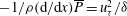 $-1/{\it\rho}(\text{d}/\text{d}x)\overline{P}=u_{{\it\tau}}^{2}/{\it\delta}$
where
$-1/{\it\rho}(\text{d}/\text{d}x)\overline{P}=u_{{\it\tau}}^{2}/{\it\delta}$
where
 ${\it\delta}$
is the half-width of the channel or the radius of the pipe, allows determination of the skin friction velocity
${\it\delta}$
is the half-width of the channel or the radius of the pipe, allows determination of the skin friction velocity
 $u_{{\it\tau}}$
from measurements of the mean pressure gradient
$u_{{\it\tau}}$
from measurements of the mean pressure gradient
 $-(\text{d}/\text{d}x)\overline{P}$
(
$-(\text{d}/\text{d}x)\overline{P}$
(
 ${\it\rho}$
is the mass density of the fluid).
${\it\rho}$
is the mass density of the fluid).
The wall unit is
 ${\it\delta}_{{\it\nu}}\equiv {\it\nu}/u_{{\it\tau}}$
. It is well known that if the Reynolds number is large enough, then
${\it\delta}_{{\it\nu}}\equiv {\it\nu}/u_{{\it\tau}}$
. It is well known that if the Reynolds number is large enough, then
 ${\it\delta}_{{\it\nu}}\ll {\it\delta}$
, e.g. see Pope (Reference Pope2000). In such flows, one often uses the Reynolds number
${\it\delta}_{{\it\nu}}\ll {\it\delta}$
, e.g. see Pope (Reference Pope2000). In such flows, one often uses the Reynolds number
 $\mathit{Re}_{{\it\tau}}\equiv {\it\delta}/{\it\delta}_{{\it\nu}}$
as reference. High Reynolds number then trivially implies wide separation of outer/inner length scales and an intermediate layer
$\mathit{Re}_{{\it\tau}}\equiv {\it\delta}/{\it\delta}_{{\it\nu}}$
as reference. High Reynolds number then trivially implies wide separation of outer/inner length scales and an intermediate layer
 ${\it\delta}_{{\it\nu}}\ll y\ll {\it\delta}$
where
${\it\delta}_{{\it\nu}}\ll y\ll {\it\delta}$
where
 $y$
is the wall-normal spatial coordinate with
$y$
is the wall-normal spatial coordinate with
 $y=0$
at the wall.
$y=0$
at the wall.
For a given channel/pipe (i.e. a given
 ${\it\delta}$
), a given fluid (i.e. a given kinematic viscosity
${\it\delta}$
), a given fluid (i.e. a given kinematic viscosity
 ${\it\nu}$
), a given driving pressure drop (i.e. a given
${\it\nu}$
), a given driving pressure drop (i.e. a given
 $u_{{\it\tau}}$
) and at a given distance
$u_{{\it\tau}}$
) and at a given distance
 $y$
from the wall, a streamwise wavenumber
$y$
from the wall, a streamwise wavenumber
 $k_{1}$
could be comparable to
$k_{1}$
could be comparable to
 $1/{\it\delta}$
,
$1/{\it\delta}$
,
 $1/y$
,
$1/y$
,
 $1/{\it\eta}$
or
$1/{\it\eta}$
or
 $1/{\it\delta}_{{\it\nu}}$
(
$1/{\it\delta}_{{\it\nu}}$
(
 ${\it\eta}\equiv ({\it\nu}^{3}/{\it\epsilon})^{1/4}$
is the Kolmogorov microscale which is a function of
${\it\eta}\equiv ({\it\nu}^{3}/{\it\epsilon})^{1/4}$
is the Kolmogorov microscale which is a function of
 $y$
via its dependence on kinetic energy dissipation rate per unit mass
$y$
via its dependence on kinetic energy dissipation rate per unit mass
 ${\it\epsilon}$
).
${\it\epsilon}$
).
The argument which shows that
 ${\it\delta}_{{\it\nu}}$
is smaller than
${\it\delta}_{{\it\nu}}$
is smaller than
 ${\it\eta}$
is based on the log-law of the wall and on the direct balance between production and dissipation which one classically expects in the
${\it\eta}$
is based on the log-law of the wall and on the direct balance between production and dissipation which one classically expects in the
 $y$
-region where the Prandtl–von Kármán law of the wall holds, e.g. see Townsend (Reference Townsend1976) and Pope (Reference Pope2000). At extremely high
$y$
-region where the Prandtl–von Kármán law of the wall holds, e.g. see Townsend (Reference Townsend1976) and Pope (Reference Pope2000). At extremely high
 $\mathit{Re}_{{\it\tau}}$
, this balance may be written as
$\mathit{Re}_{{\it\tau}}$
, this balance may be written as
 $u_{{\it\tau}}^{2}(\text{d}/\text{d}y)\overline{u}\approx {\it\epsilon}$
where we have replaced the Reynolds stress by
$u_{{\it\tau}}^{2}(\text{d}/\text{d}y)\overline{u}\approx {\it\epsilon}$
where we have replaced the Reynolds stress by
 $u_{{\it\tau}}^{2}$
. It can be proved that the Reynolds shear stress is approximately equal to
$u_{{\it\tau}}^{2}$
. It can be proved that the Reynolds shear stress is approximately equal to
 $u_{{\it\tau}}^{2}$
in the range
$u_{{\it\tau}}^{2}$
in the range
 ${\it\delta}_{{\it\nu}}\ll y\ll {\it\delta}$
. This follows from the turbulent pipe flow axial momentum balance and a very mild extra assumption, see § 3 of Dallas, Vassilicos & Hewitt (Reference Dallas, Vassilicos and Hewitt2009).
${\it\delta}_{{\it\nu}}\ll y\ll {\it\delta}$
. This follows from the turbulent pipe flow axial momentum balance and a very mild extra assumption, see § 3 of Dallas, Vassilicos & Hewitt (Reference Dallas, Vassilicos and Hewitt2009).
This equilibrium argument implies that
 ${\it\epsilon}\sim u_{{\it\tau}}^{3}/y$
(assuming that the log-law
${\it\epsilon}\sim u_{{\it\tau}}^{3}/y$
(assuming that the log-law
 $(\text{d}/\text{d}y)\overline{u}\sim u_{{\it\tau}}/y$
holds) in
$(\text{d}/\text{d}y)\overline{u}\sim u_{{\it\tau}}/y$
holds) in
 ${\it\delta}_{{\it\nu}}\ll y\ll {\it\delta}$
. It is now possible to compare
${\it\delta}_{{\it\nu}}\ll y\ll {\it\delta}$
. It is now possible to compare
 ${\it\eta}=({\it\nu}^{3}/{\it\epsilon})^{1/4}$
and
${\it\eta}=({\it\nu}^{3}/{\it\epsilon})^{1/4}$
and
 ${\it\delta}_{{\it\nu}}={\it\nu}/u_{{\it\tau}}$
and it follows from
${\it\delta}_{{\it\nu}}={\it\nu}/u_{{\it\tau}}$
and it follows from
 ${\it\delta}_{{\it\nu}}\ll y$
that
${\it\delta}_{{\it\nu}}\ll y$
that
 $1/{\it\eta}\ll 1/{\it\delta}_{{\it\nu}}$
in the range
$1/{\it\eta}\ll 1/{\it\delta}_{{\it\nu}}$
in the range
 ${\it\delta}_{{\it\nu}}\ll y\ll {\it\delta}$
. It is worth stressing that
${\it\delta}_{{\it\nu}}\ll y\ll {\it\delta}$
. It is worth stressing that
 $1/{\it\eta}\ll 1/{\it\delta}_{{\it\nu}}$
and
$1/{\it\eta}\ll 1/{\it\delta}_{{\it\nu}}$
and
 ${\it\epsilon}\sim u_{{\it\tau}}^{3}/y$
were obtained on the basis that the range
${\it\epsilon}\sim u_{{\it\tau}}^{3}/y$
were obtained on the basis that the range
 ${\it\delta}_{{\it\nu}}\ll y\ll {\it\delta}$
is an equilibrium log-law range in a pipe flow. We revisit this assumption in § 6.
${\it\delta}_{{\it\nu}}\ll y\ll {\it\delta}$
is an equilibrium log-law range in a pipe flow. We revisit this assumption in § 6.
From the above arguments, where
 $y$
is much larger than
$y$
is much larger than
 ${\it\delta}_{{\it\nu}}$
but much smaller than
${\it\delta}_{{\it\nu}}$
but much smaller than
 ${\it\delta}$
, the axis of wavenumbers
${\it\delta}$
, the axis of wavenumbers
 $k_{1}$
is marked by wavenumbers
$k_{1}$
is marked by wavenumbers
 $1/{\it\delta}$
,
$1/{\it\delta}$
,
 $1/y$
,
$1/y$
,
 $1/{\it\eta}$
and
$1/{\it\eta}$
and
 $1/{\it\delta}_{{\it\nu}}$
in this increasing wavenumber order. This order of cross-over wavenumbers is important in the spectral interpretation given by Perry et al. (Reference Perry, Henbest and Chong1986) of Townsend’s attached eddy hypothesis.
$1/{\it\delta}_{{\it\nu}}$
in this increasing wavenumber order. This order of cross-over wavenumbers is important in the spectral interpretation given by Perry et al. (Reference Perry, Henbest and Chong1986) of Townsend’s attached eddy hypothesis.
3. The Townsend–Perry attached eddy model
Townsend (Reference Townsend1976) assumed ‘that the main, energy-containing motion is made up of contributions from “attached” eddies with similar velocity distributions’ and developed a physical space argument based on the notion of a constant Reynolds shear stress which led to
 $$\begin{eqnarray}{\textstyle \frac{1}{2}}\overline{u^{\prime 2}}(y)/u_{{\it\tau}}^{2}\approx C_{s0}+C_{s1}\ln ({\it\delta}/y)\end{eqnarray}$$
in the range
 ${\it\delta}_{{\it\nu}}\ll y\ll {\it\delta}$
. The two constants
${\it\delta}_{{\it\nu}}\ll y\ll {\it\delta}$
. The two constants
 $C_{s0}$
and
$C_{s0}$
and
 $C_{s1}$
are independent of
$C_{s1}$
are independent of
 $y$
and
$y$
and
 $\mathit{Re}_{{\it\tau}}$
.
$\mathit{Re}_{{\it\tau}}$
.
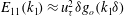
Perry et al. (Reference Perry, Henbest and Chong1986) developed a spectral attached eddy model and argued that where
 ${\it\delta}_{{\it\nu}}\ll y\ll {\it\delta}$
, the streamwise energy spectrum
${\it\delta}_{{\it\nu}}\ll y\ll {\it\delta}$
, the streamwise energy spectrum
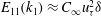
 $E_{11}(k_{1},y)$
has three distinct ranges:
$E_{11}(k_{1},y)$
has three distinct ranges:
-
(i)
 $k_{1}<1/{\it\delta}$
where
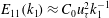
$E_{11}(k_{1})\approx u_{{\it\tau}}^{2}{\it\delta}g_{o}(k_{1}{\it\delta})$
which must be
$E_{11}(k_{1})\approx C_{\infty }u_{{\it\tau}}^{2}{\it\delta}$
with a constant
$C_{\infty }$
at small enough wavenumbers;
$k_{1}<1/{\it\delta}$
where
$E_{11}(k_{1})\approx u_{{\it\tau}}^{2}{\it\delta}g_{o}(k_{1}{\it\delta})$
which must be
$E_{11}(k_{1})\approx C_{\infty }u_{{\it\tau}}^{2}{\it\delta}$
with a constant
$C_{\infty }$
at small enough wavenumbers; -
(ii)
$1/{\it\delta}<k_{1}<1/y$
where
$E_{11}(k_{1})\approx C_{0}u_{{\it\tau}}^{2}k_{1}^{-1}$
(the ‘attached eddy’ range); -
(iii)
$1/y<k_{1}$
where
$E_{11}(k_{1})$
has the Kolmogorov form
$E_{11}(k_{1},y)\sim {\it\epsilon}^{2/3}k_{1}^{-5/3}g_{K}(k_{1}y,k_{1}{\it\eta})$
, see Frisch (Reference Frisch1995) and Pope (Reference Pope2000).


By integration of
 $E_{11}(k_{1})$
they obtained for
$E_{11}(k_{1})$
they obtained for
 ${\it\delta}_{{\it\nu}}\ll y\ll {\it\delta}$
 $$\begin{eqnarray}{\textstyle \frac{1}{2}}\overline{u^{\prime 2}}(y)/u_{{\it\tau}}^{2}\approx C_{\infty }+C_{0}\ln ({\it\delta}/y)\end{eqnarray}$$
where the constants
 $C_{\infty }$
and
$C_{\infty }$
and
 $C_{0}$
are independent of
$C_{0}$
are independent of
 $y$
and
$y$
and
 $\mathit{Re}_{{\it\tau}}$
. Application of a strict matching condition for the energy spectra at
$\mathit{Re}_{{\it\tau}}$
. Application of a strict matching condition for the energy spectra at
 $k_{1}=1/{\it\delta}$
gives
$k_{1}=1/{\it\delta}$
gives
 $C_{0}=C_{\infty }$
but this is of course not necessary. In fact, the constant
$C_{0}=C_{\infty }$
but this is of course not necessary. In fact, the constant
 $C_{\infty }$
in (3.2) is not the same as the constant
$C_{\infty }$
in (3.2) is not the same as the constant
 $C_{\infty }$
in the spectral model if we allow for the wavenumber dependency of the outer function
$C_{\infty }$
in the spectral model if we allow for the wavenumber dependency of the outer function
 $g_{o}(k_{1}y)$
and for the fact that this constant has a small contribution from the high-wavenumber Kolmogorov range (iii). The detail of this Kolmogorov contribution has been neglected in (3.2) as it only adds a term proportional to
$g_{o}(k_{1}y)$
and for the fact that this constant has a small contribution from the high-wavenumber Kolmogorov range (iii). The detail of this Kolmogorov contribution has been neglected in (3.2) as it only adds a term proportional to
 $1-(y^{+})^{-1/2}$
to the right-hand side (
$1-(y^{+})^{-1/2}$
to the right-hand side (
 $y^{+}\equiv y/{\it\delta}_{{\it\nu}}$
) which is of little effect in the considered range.
$y^{+}\equiv y/{\it\delta}_{{\it\nu}}$
) which is of little effect in the considered range.
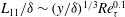
A consequence of the Perry et al. (Reference Perry, Henbest and Chong1986) model is that the integral scale
 $L_{11}$
is proportional to
$L_{11}$
is proportional to
 ${\it\delta}$
and very weakly dependent on
${\it\delta}$
and very weakly dependent on
 $y$
in the intermediate layer
$y$
in the intermediate layer
 ${\it\delta}_{{\it\nu}}\ll y\ll {\it\delta}$
. This follows from
${\it\delta}_{{\it\nu}}\ll y\ll {\it\delta}$
. This follows from
 ${\rm\pi}E_{11}(k_{1}=0,y)=\overline{u^{\prime 2}}(y)L_{11}(y)$
(see e.g. Tennekes & Lumley Reference Tennekes and Lumley1972) which leads to
${\rm\pi}E_{11}(k_{1}=0,y)=\overline{u^{\prime 2}}(y)L_{11}(y)$
(see e.g. Tennekes & Lumley Reference Tennekes and Lumley1972) which leads to
 $$\begin{eqnarray}L_{11}(y)\approx \frac{{\rm\pi}C_{\infty }{\it\delta}}{C_{\infty }+C_{0}\ln ({\it\delta}/y)}\end{eqnarray}$$
where
 ${\it\delta}_{{\it\nu}}\ll y\ll {\it\delta}$
. However, one expects that
${\it\delta}_{{\it\nu}}\ll y\ll {\it\delta}$
. However, one expects that
 $L_{11}$
may depend on
$L_{11}$
may depend on
 $y$
much more steeply. For example, the turbulent boundary layer measurements of Tomkins & Adrian (Reference Tomkins and Adrian2003) suggest that
$y$
much more steeply. For example, the turbulent boundary layer measurements of Tomkins & Adrian (Reference Tomkins and Adrian2003) suggest that
 $L_{11}\sim y$
.
$L_{11}\sim y$
.
The only way for the Townsend–Perry attached eddy wavenumber range to be viable, i.e. the only way to have an integral scale which depends more substantially on
 $y$
while keeping with the Townsend–Perry attached eddy wavenumber range (where, in particular, the constant
$y$
while keeping with the Townsend–Perry attached eddy wavenumber range (where, in particular, the constant
 $C_{0}$
is independent of
$C_{0}$
is independent of
 $y$
and
$y$
and
 $\mathit{Re}_{{\it\tau}}$
) is to modify the model of Perry et al. (Reference Perry, Henbest and Chong1986) by inserting a fourth range to
$\mathit{Re}_{{\it\tau}}$
) is to modify the model of Perry et al. (Reference Perry, Henbest and Chong1986) by inserting a fourth range to
 $E_{11}(k_{1})$
between the very low-wavenumber range where
$E_{11}(k_{1})$
between the very low-wavenumber range where
 $E_{11}(k_{1})\approx C_{\infty }u_{{\it\tau}}^{2}{\it\delta}$
and the ‘attached eddy’ range. We develop such a model in the following section.
$E_{11}(k_{1})\approx C_{\infty }u_{{\it\tau}}^{2}{\it\delta}$
and the ‘attached eddy’ range. We develop such a model in the following section.
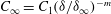
4. A modified Townsend–Perry attached eddy model
We now consider a model of the energy spectrum
 $E_{11}(k_{1},y)$
with the following four ranges (see figure 1)
$E_{11}(k_{1},y)$
with the following four ranges (see figure 1)
-
(i)
$k_{1}\!<1/{\it\delta}_{\infty }$
where
$E_{11}(k_{1})\!\approx C_{\infty }u_{{\it\tau}}^{2}{\it\delta}$
with a constant
$C_{\infty }$
independent of wavenumber; -
(ii)
$1/{\it\delta}_{\infty }<k_{1}<1/{\it\delta}_{\ast }$
where
$E_{11}(k_{1})\approx C_{1}u_{{\it\tau}}^{2}{\it\delta}(k_{1}{\it\delta})^{-m}$
where
$0<m<1$
and
$C_{1}$
is also a constant independent of wavenumber; -
(iii)
$1/{\it\delta}_{\ast }<k_{1}<1/y$
where
$E_{11}(k_{1})\approx C_{0}u_{{\it\tau}}^{2}k_{1}^{-1}$
where
$C_{0}$
is a constant independent of wavenumber,
$y$
and
$\mathit{Re}_{{\it\tau}}$
(the ‘attached eddy’ range); -
(iv)
$1/y<k_{1}$
where
$E_{11}(k_{1})$
has the Kolmogorov form
$E_{11}(k_{1},y)\sim {\it\epsilon}^{2/3}k_{1}^{-5/3}g_{K}(k_{1}y,k_{1}{\it\eta})$
.


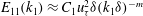


Schematic log–log plot of
 $E_{11}(k_{1})/u_{{\it\tau}}^{2}$
versus
$E_{11}(k_{1})/u_{{\it\tau}}^{2}$
versus
 $k_{1}$
according to the modified Townsend–Perry attached eddy model for the region
$k_{1}$
according to the modified Townsend–Perry attached eddy model for the region
 ${\it\delta}_{{\it\nu}}\ll y\ll {\it\delta}$
. Given an ansatz such as (4.1) with
${\it\delta}_{{\it\nu}}\ll y\ll {\it\delta}$
. Given an ansatz such as (4.1) with
 $p,q>0$
and
$p,q>0$
and
 $p>q$
set by the physics described in the second and third paragraphs of § 4, the new range (ii) exists where
$p>q$
set by the physics described in the second and third paragraphs of § 4, the new range (ii) exists where
 $y<y_{\ast }$
, in which case
$y<y_{\ast }$
, in which case
 ${\it\delta}_{\ast }<{\it\delta}_{\infty }$
, but does not exist where
${\it\delta}_{\ast }<{\it\delta}_{\infty }$
, but does not exist where
 $y>y_{\ast }$
in which case the original Townsend–Perry model remains unaltered and
$y>y_{\ast }$
in which case the original Townsend–Perry model remains unaltered and
 ${\it\delta}_{\ast }={\it\delta}_{\infty }={\it\delta}$
.
${\it\delta}_{\ast }={\it\delta}_{\infty }={\it\delta}$
.

The new range which is dictated by the requirement of an integral scale significantly dependent on
 $y$
is range (ii) and it lies, as is necessary for this requirement, between ranges (i) and the ‘attached eddy’ range (iii). This range therefore corresponds to rather large length scales which may naturally be expected to be the large and very large-scale motions first discovered by Tomkins & Adrian (Reference Tomkins and Adrian2003) and confirmed for a range of Reynolds numbers by Hutchins & Marusic (Reference Hutchins and Marusic2007) (see also Bailey & Smits Reference Bailey and Smits2010 in the present pipe flow context and the review of Smits et al.
Reference Smits, McKeon and Marusic2011). Indeed, such long regions of momentum deficit elongated in the streamwise direction should introduce long-range correlations in this direction. These long-range correlations will appear as a range of reduced rate of decline at the higher separation distances of the streamwise fluctuating velocity autocorrelation function which, when Fourier transformed, will give rise to a range such as range (ii) in the energy spectrum.
$y$
is range (ii) and it lies, as is necessary for this requirement, between ranges (i) and the ‘attached eddy’ range (iii). This range therefore corresponds to rather large length scales which may naturally be expected to be the large and very large-scale motions first discovered by Tomkins & Adrian (Reference Tomkins and Adrian2003) and confirmed for a range of Reynolds numbers by Hutchins & Marusic (Reference Hutchins and Marusic2007) (see also Bailey & Smits Reference Bailey and Smits2010 in the present pipe flow context and the review of Smits et al.
Reference Smits, McKeon and Marusic2011). Indeed, such long regions of momentum deficit elongated in the streamwise direction should introduce long-range correlations in this direction. These long-range correlations will appear as a range of reduced rate of decline at the higher separation distances of the streamwise fluctuating velocity autocorrelation function which, when Fourier transformed, will give rise to a range such as range (ii) in the energy spectrum.
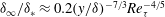
The bounds of the new range (ii) are determined by the two new length scales
 ${\it\delta}_{\infty }$
and
${\it\delta}_{\infty }$
and
 ${\it\delta}_{\ast }$
. The only physics that we impose on them is the expectation that this range grows as
${\it\delta}_{\ast }$
. The only physics that we impose on them is the expectation that this range grows as
 $y$
approaches the wall and distances itself from the centre of the pipe within
$y$
approaches the wall and distances itself from the centre of the pipe within
 ${\it\delta}_{{\it\nu}}\ll y\ll {\it\delta}$
. The range
${\it\delta}_{{\it\nu}}\ll y\ll {\it\delta}$
. The range
 $(1/{\it\delta}_{\ast })/(1/{\it\delta}_{\infty })={\it\delta}_{\infty }/{\it\delta}_{\ast }$
can only depend on
$(1/{\it\delta}_{\ast })/(1/{\it\delta}_{\infty })={\it\delta}_{\infty }/{\it\delta}_{\ast }$
can only depend on
 $y$
,
$y$
,
 ${\it\delta}$
,
${\it\delta}$
,
 ${\it\nu}$
and
${\it\nu}$
and
 $u_{{\it\tau}}$
. Without loss of generality, it is therefore a function of
$u_{{\it\tau}}$
. Without loss of generality, it is therefore a function of
 $y/{\it\delta}$
and
$y/{\it\delta}$
and
 $\mathit{Re}_{{\it\tau}}$
or, equivalently,
$\mathit{Re}_{{\it\tau}}$
or, equivalently,
 $y^{+}$
and
$y^{+}$
and
 $\mathit{Re}_{{\it\tau}}$
. At fixed
$\mathit{Re}_{{\it\tau}}$
. At fixed
 $\mathit{Re}_{{\it\tau}}$
,
$\mathit{Re}_{{\it\tau}}$
,
 ${\it\delta}_{\infty }/{\it\delta}_{\ast }$
must be a decreasing function of
${\it\delta}_{\infty }/{\it\delta}_{\ast }$
must be a decreasing function of
 $y/{\it\delta}$
and also a decreasing function of
$y/{\it\delta}$
and also a decreasing function of
 $y^{+}$
. At fixed
$y^{+}$
. At fixed
 $y/{\it\delta}$
,
$y/{\it\delta}$
,
 ${\it\delta}_{\infty }/{\it\delta}_{\ast }$
must be a decreasing function of
${\it\delta}_{\infty }/{\it\delta}_{\ast }$
must be a decreasing function of
 $\mathit{Re}_{{\it\tau}}$
as this implies that
$\mathit{Re}_{{\it\tau}}$
as this implies that
 $y^{+}$
increases. And at fixed
$y^{+}$
increases. And at fixed
 $y^{+}$
,
$y^{+}$
,
 ${\it\delta}_{\infty }/{\it\delta}_{\ast }$
must be an increasing function of
${\it\delta}_{\infty }/{\it\delta}_{\ast }$
must be an increasing function of
 $\mathit{Re}_{{\it\tau}}$
as this means that
$\mathit{Re}_{{\it\tau}}$
as this means that
 $y/{\it\delta}$
decreases.
$y/{\it\delta}$
decreases.
An arbitrary but not impossible functional dependence is
 $$\begin{eqnarray}{\it\delta}_{\infty }/{\it\delta}_{\ast }\approx A\;(y/{\it\delta})^{-p}\mathit{Re}_{{\it\tau}}^{-q}\approx A(y^{+})^{-p}{\mathit{Re}_{{\it\tau}}}^{p-q}\end{eqnarray}$$
where
 $A$
is a dimensionless constant. The qualitative physics which we described in the previous paragraph impose
$A$
is a dimensionless constant. The qualitative physics which we described in the previous paragraph impose
 $p,q>0$
and
$p,q>0$
and
 $p>q$
. We adopt (4.1) indicatively in what follows as the aim of this work is to show the possibilities which open up with the adoption of the extra wavenumber range
$p>q$
. We adopt (4.1) indicatively in what follows as the aim of this work is to show the possibilities which open up with the adoption of the extra wavenumber range
 $1/{\it\delta}_{\infty }<k_{1}<1/{\it\delta}_{\ast }$
for the purpose of reconciling the Townsend–Perry attached eddy hypothesis with a more realistic integral length scale. We limit the values of the exponents
$1/{\it\delta}_{\infty }<k_{1}<1/{\it\delta}_{\ast }$
for the purpose of reconciling the Townsend–Perry attached eddy hypothesis with a more realistic integral length scale. We limit the values of the exponents
 $p$
and
$p$
and
 $q$
to
$q$
to
 $p,q>0$
and
$p,q>0$
and
 $p>q$
without further constraints.
$p>q$
without further constraints.
Matching of the energy spectral forms at
 $k_{1}\approx 1/{\it\delta}_{\infty }$
gives
$k_{1}\approx 1/{\it\delta}_{\infty }$
gives
 $C_{\infty }=C_{1}({\it\delta}/{\it\delta}_{\infty })^{-m}$
and at
$C_{\infty }=C_{1}({\it\delta}/{\it\delta}_{\infty })^{-m}$
and at
 $k_{1}\approx 1/{\it\delta}_{\ast }$
gives
$k_{1}\approx 1/{\it\delta}_{\ast }$
gives
 $C_{1}=C_{0}({\it\delta}/{\it\delta}_{\ast })^{m-1}$
. It is not strictly necessary to impose these matching conditions as they unnecessarily restrict the cross-over forms of the energy spectra, but they do indicate that we need an expression for
$C_{1}=C_{0}({\it\delta}/{\it\delta}_{\ast })^{m-1}$
. It is not strictly necessary to impose these matching conditions as they unnecessarily restrict the cross-over forms of the energy spectra, but they do indicate that we need an expression for
 ${\it\delta}_{\ast }/{\it\delta}$
if we are to proceed with or without them. Given that in all generality,
${\it\delta}_{\ast }/{\it\delta}$
if we are to proceed with or without them. Given that in all generality,
 ${\it\delta}_{\ast }/{\it\delta}$
is a function of
${\it\delta}_{\ast }/{\it\delta}$
is a function of
 $y/{\it\delta}$
and
$y/{\it\delta}$
and
 $\mathit{Re}_{{\it\tau}}$
, we again assume a power-law form
$\mathit{Re}_{{\it\tau}}$
, we again assume a power-law form
 $$\begin{eqnarray}{\it\delta}_{\ast }/{\it\delta}=B\;(y/{\it\delta})^{{\it\alpha}}\mathit{Re}_{{\it\tau}}^{{\it\beta}}\end{eqnarray}$$
where, like
 $A$
,
$A$
,
 $B$
is a dimensionless constant.
$B$
is a dimensionless constant.
There are also two requirements for the viability of our spectra:
 $y\ll {\it\delta}_{\ast }$
and
$y\ll {\it\delta}_{\ast }$
and
 ${\it\delta}_{\ast }<{\it\delta}_{\infty }$
. The former is met provided that
${\it\delta}_{\ast }<{\it\delta}_{\infty }$
. The former is met provided that
 ${\it\beta}\geqslant {\it\alpha}-1$
for
${\it\beta}\geqslant {\it\alpha}-1$
for
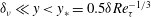
 $y\gg {\it\delta}_{{\it\nu}}$
. The latter is met if
$y\gg {\it\delta}_{{\it\nu}}$
. The latter is met if
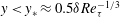
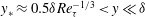
 $y<y_{\ast }\equiv {\it\delta}A^{1/p}\mathit{Re}_{{\it\tau}}^{-q/p}$
.
$y<y_{\ast }\equiv {\it\delta}A^{1/p}\mathit{Re}_{{\it\tau}}^{-q/p}$
.
We therefore adopt the new range (ii) for
 $y<y_{\ast }$
but keep the Perry et al. (Reference Perry, Henbest and Chong1986) model unaltered for
$y<y_{\ast }$
but keep the Perry et al. (Reference Perry, Henbest and Chong1986) model unaltered for
 $y>y_{\ast }$
. Their model can indeed remain unaltered if
$y>y_{\ast }$
. Their model can indeed remain unaltered if
 ${\it\delta}_{\infty }={\it\delta}_{\ast }={\it\delta}$
at
${\it\delta}_{\infty }={\it\delta}_{\ast }={\it\delta}$
at
 $y\geqslant y_{\ast }={\it\delta}A^{1/p}\mathit{Re}_{{\it\tau}}^{-q/p}$
. The continuous passage from (4.1) and (4.2) to
$y\geqslant y_{\ast }={\it\delta}A^{1/p}\mathit{Re}_{{\it\tau}}^{-q/p}$
. The continuous passage from (4.1) and (4.2) to
 ${\it\delta}_{\infty }={\it\delta}_{\ast }={\it\delta}$
requires
${\it\delta}_{\infty }={\it\delta}_{\ast }={\it\delta}$
requires
 ${\it\beta}={\it\alpha}q/p$
and
${\it\beta}={\it\alpha}q/p$
and
 $BA^{{\it\alpha}/p}=1$
.
$BA^{{\it\alpha}/p}=1$
.
By integration of
 $E_{11}(k_{1})$
we obtain for
$E_{11}(k_{1})$
we obtain for
 ${\it\delta}_{{\it\nu}}\ll y\leqslant y_{\ast }$
 $$\begin{eqnarray}{\textstyle \frac{1}{2}}\overline{u^{\prime 2}}(y)/u_{{\it\tau}}^{2}\approx C_{s0}-C_{s1}\ln ({\it\delta}/y)-C_{s2}(y/{\it\delta})^{p(1-m)}\mathit{Re}_{{\it\tau}}^{q(1-m)}\end{eqnarray}$$
where
 $C_{s0}=(C_{0}/(1-m))+C_{0}\ln B+C_{0}{\it\alpha}(q/p)\ln \mathit{Re}_{{\it\tau}}$
,
$C_{s0}=(C_{0}/(1-m))+C_{0}\ln B+C_{0}{\it\alpha}(q/p)\ln \mathit{Re}_{{\it\tau}}$
,
 $C_{s1}=C_{0}({\it\alpha}-1)$
and
$C_{s1}=C_{0}({\it\alpha}-1)$
and
 $C_{s2}=(mC_{0}A^{m-1})/(1-m)$
. (Note that
$C_{s2}=(mC_{0}A^{m-1})/(1-m)$
. (Note that
 $C_{s0}$
is a weak function of
$C_{s0}$
is a weak function of
 $\mathit{Re}_{{\it\tau}}$
whereas
$\mathit{Re}_{{\it\tau}}$
whereas
 $C_{s1}$
and
$C_{s1}$
and
 $C_{s2}$
are independent of
$C_{s2}$
are independent of
 $\mathit{Re}_{{\it\tau}}$
.) These new constants have been calculated by taking into account the perhaps over-constraining matching conditions
$\mathit{Re}_{{\it\tau}}$
.) These new constants have been calculated by taking into account the perhaps over-constraining matching conditions
 $C_{\infty }=C_{1}({\it\delta}/{\it\delta}_{\infty })^{-m}$
and
$C_{\infty }=C_{1}({\it\delta}/{\it\delta}_{\infty })^{-m}$
and
 $C_{1}=C_{0}({\it\delta}/{\it\delta}_{\ast })^{m-1}$
.
$C_{1}=C_{0}({\it\delta}/{\it\delta}_{\ast })^{m-1}$
.
The integral length scale is now
 $$\begin{eqnarray}L_{11}/{\it\delta}={\rm\pi}C_{0}A^{m}B(y/{\it\delta})^{{\it\alpha}-pm}\mathit{Re}_{{\it\tau}}^{{\it\beta}-qm}/(\overline{u^{\prime 2}}(y)/u_{{\it\tau}}^{2})\end{eqnarray}$$
clearly more strongly dependent on
 $y$
than in (3.3).
$y$
than in (3.3).
Equation (4.3) can be compared with the Townsend–Perry form which remains valid here for
 $y_{\ast }\leqslant y\ll {\it\delta}$
and which is (taking
$y_{\ast }\leqslant y\ll {\it\delta}$
and which is (taking
 $C_{\infty }=C_{0}$
)
$C_{\infty }=C_{0}$
)
 $$\begin{eqnarray}{\textstyle \frac{1}{2}}\overline{u^{\prime 2}}(y)/u_{{\it\tau}}^{2}\approx C_{0}+C_{0}\ln ({\it\delta}/y).\end{eqnarray}$$
The two profiles (4.3) and (4.5) match at
 $y=y_{\ast }\equiv {\it\delta}A^{1/p}\mathit{Re}_{{\it\tau}}^{-q/p}$
and so do also the integral length-scale forms (4.4) and (3.3) if
$y=y_{\ast }\equiv {\it\delta}A^{1/p}\mathit{Re}_{{\it\tau}}^{-q/p}$
and so do also the integral length-scale forms (4.4) and (3.3) if
 $C_{\infty }=C_{0}$
. Our approach does not modify the Townsend–Perry form of
$C_{\infty }=C_{0}$
. Our approach does not modify the Townsend–Perry form of
 $L_{11}$
at large distances from the wall, i.e. at
$L_{11}$
at large distances from the wall, i.e. at
 $y>y_{\ast }$
, but it does return a significant dependence of
$y>y_{\ast }$
, but it does return a significant dependence of
 $L_{11}$
on
$L_{11}$
on
 $y$
which, however, is arbitrarily set by (4.1) and (4.2). Even so, the possibility is now open for a stronger dependence of
$y$
which, however, is arbitrarily set by (4.1) and (4.2). Even so, the possibility is now open for a stronger dependence of
 $L_{11}$
on
$L_{11}$
on
 $y$
. This possibility has been opened by the adoption of an extra wavenumber range
$y$
. This possibility has been opened by the adoption of an extra wavenumber range
 $1/{\it\delta}_{\infty }<k_{1}<1/{\it\delta}_{\ast }$
which, in turn, returns a form of the
$1/{\it\delta}_{\infty }<k_{1}<1/{\it\delta}_{\ast }$
which, in turn, returns a form of the
 $\overline{u^{\prime 2}}(y)$
profile which allows for a maximum value (a peak) inside the intermediate region
$\overline{u^{\prime 2}}(y)$
profile which allows for a maximum value (a peak) inside the intermediate region
 ${\it\delta}_{{\it\nu}}\ll y\ll {\it\delta}$
. No such peak is allowed by the Townsend–Perry forms (3.1) and (3.2) although such a peak has been observed in measurements of both turbulent boundary layers and turbulent pipe flows over the past 20 years or so, see Fernholz & Finley (Reference Fernholz and Finley1996), Morrison et al. (Reference Morrison, McKeon, Jiang and Smits2004) and Hultmark et al. (Reference Hultmark, Vallikivi, Bailey and Smits2012, Reference Hultmark, Vallikivi, Bailey and Smits2013). It has been suggested that this peak is associated with the large and very large motions (see Smits et al.
Reference Smits, McKeon and Marusic2011 and references therein) which is consistent with the view that the wavenumber range
${\it\delta}_{{\it\nu}}\ll y\ll {\it\delta}$
. No such peak is allowed by the Townsend–Perry forms (3.1) and (3.2) although such a peak has been observed in measurements of both turbulent boundary layers and turbulent pipe flows over the past 20 years or so, see Fernholz & Finley (Reference Fernholz and Finley1996), Morrison et al. (Reference Morrison, McKeon, Jiang and Smits2004) and Hultmark et al. (Reference Hultmark, Vallikivi, Bailey and Smits2012, Reference Hultmark, Vallikivi, Bailey and Smits2013). It has been suggested that this peak is associated with the large and very large motions (see Smits et al.
Reference Smits, McKeon and Marusic2011 and references therein) which is consistent with the view that the wavenumber range
 $1/{\it\delta}_{\infty }<k_{1}<1/{\it\delta}_{\ast }$
results from these very elongated streamwise structures.
$1/{\it\delta}_{\infty }<k_{1}<1/{\it\delta}_{\ast }$
results from these very elongated streamwise structures.
Straightforward analysis of (4.3) shows that a maximum streamwise turbulence intensity does exist in the range
 ${\it\delta}_{{\it\nu}}\ll y\ll {\it\delta}$
if
${\it\delta}_{{\it\nu}}\ll y\ll {\it\delta}$
if
 $0<{\it\alpha}-1<pm$
(i.e. if
$0<{\it\alpha}-1<pm$
(i.e. if
 $C_{s1}>0$
and
$C_{s1}>0$
and
 ${\it\alpha}<pm+1$
) and that the position
${\it\alpha}<pm+1$
) and that the position
 $y_{peak}$
of this maximum is
$y_{peak}$
of this maximum is
 $$\begin{eqnarray}y_{peak}/{\it\delta}\sim \mathit{Re}_{{\it\tau}}^{-q/p}\end{eqnarray}$$
which decreases with increasing
 $\mathit{Re}_{{\it\tau}}$
and, equivalently,
$\mathit{Re}_{{\it\tau}}$
and, equivalently,
 $$\begin{eqnarray}y_{peak}/{\it\delta}_{{\it\nu}}\sim \mathit{Re}_{{\it\tau}}^{1-q/p}\end{eqnarray}$$
which increases with increasing
 $\mathit{Re}_{{\it\tau}}$
as
$\mathit{Re}_{{\it\tau}}$
as
 $q<p$
. It also follows from (4.3) that
$q<p$
. It also follows from (4.3) that
 $$\begin{eqnarray}\frac{\text{d}}{\text{d}\ln \mathit{Re}_{{\it\tau}}}\left(\frac{1}{2}\overline{u^{\prime 2}}(y_{peak})/u_{{\it\tau}}^{2}\right)\approx C_{0}({\it\alpha}p/q-{\it\alpha}q/p+q/p)>0.\end{eqnarray}$$
The maximum value of
 $\overline{u^{\prime 2}}(y)/u_{{\it\tau}}^{2}$
at
$\overline{u^{\prime 2}}(y)/u_{{\it\tau}}^{2}$
at
 $y=y_{peak}$
therefore grows logarithmically with increasing
$y=y_{peak}$
therefore grows logarithmically with increasing
 $\mathit{Re}_{{\it\tau}}$
.
$\mathit{Re}_{{\it\tau}}$
.
We now compare our functional dependence of
 $(\overline{u^{\prime 2}}(y)/2)/u_{{\it\tau}}^{2}$
on
$(\overline{u^{\prime 2}}(y)/2)/u_{{\it\tau}}^{2}$
on
 $y$
and
$y$
and
 $\mathit{Re}_{{\it\tau}}$
with smooth wall turbulent pipe flow data obtained recently with a new NSTAP by Hultmark et al. (Reference Hultmark, Vallikivi, Bailey and Smits2012, Reference Hultmark, Vallikivi, Bailey and Smits2013). Below we refer to this data as NSTAP Superpipe data.
$\mathit{Re}_{{\it\tau}}$
with smooth wall turbulent pipe flow data obtained recently with a new NSTAP by Hultmark et al. (Reference Hultmark, Vallikivi, Bailey and Smits2012, Reference Hultmark, Vallikivi, Bailey and Smits2013). Below we refer to this data as NSTAP Superpipe data.
We start by fitting the data with (4.5) in the range
 $y_{\ast }<y\ll {\it\delta}$
and
$y_{\ast }<y\ll {\it\delta}$
and
 $$\begin{eqnarray}{\textstyle \frac{1}{2}}\overline{u^{\prime 2}}(y)/u_{{\it\tau}}^{2}\approx C_{s0}-C_{s1}\ln ({\it\delta}/y)-C_{s2}(y/{\it\delta})^{d_{1}}\mathit{Re}_{{\it\tau}}^{d_{2}}\end{eqnarray}$$
instead of (4.3) in the range
 ${\it\delta}_{{\it\nu}}\ll y<y_{\ast }$
where
${\it\delta}_{{\it\nu}}\ll y<y_{\ast }$
where
 $y_{\ast }={\it\delta}\mathit{Re}_{{\it\tau}}^{-d_{2}/d_{1}}$
. This is a model where we ignore the various matching conditions which led to (4.3) with the specific relations between
$y_{\ast }={\it\delta}\mathit{Re}_{{\it\tau}}^{-d_{2}/d_{1}}$
. This is a model where we ignore the various matching conditions which led to (4.3) with the specific relations between
 $C_{s0}$
,
$C_{s0}$
,
 $C_{s1}$
and
$C_{s1}$
and
 $C_{s2}$
and the parameters
$C_{s2}$
and the parameters
 $C_{0}$
,
$C_{0}$
,
 $m$
,
$m$
,
 $p$
,
$p$
,
 $q$
,
$q$
,
 $A$
,
$A$
,
 ${\it\alpha}$
and
${\it\alpha}$
and
 $\mathit{Re}_{{\it\tau}}$
. It is also a model where we just set
$\mathit{Re}_{{\it\tau}}$
. It is also a model where we just set
 $A=1$
,
$A=1$
,
 $d_{1}=p(1-m)$
and
$d_{1}=p(1-m)$
and
 $d_{2}=q(1-m)$
so that
$d_{2}=q(1-m)$
so that
 $y_{\ast }={\it\delta}\mathit{Re}_{{\it\tau}}^{-d_{2}/d_{1}}$
. In figure 2 we show the result of this fit against the NSTAP Superpipe data and in figure 3 we show the fitting values of
$y_{\ast }={\it\delta}\mathit{Re}_{{\it\tau}}^{-d_{2}/d_{1}}$
. In figure 2 we show the result of this fit against the NSTAP Superpipe data and in figure 3 we show the fitting values of
 $C_{s0}$
,
$C_{s0}$
,
 $C_{s1}$
,
$C_{s1}$
,
 $C_{s2}$
and
$C_{s2}$
and
 $d_{1}$
and
$d_{1}$
and
 $d_{2}$
and their dependence on
$d_{2}$
and their dependence on
 $\mathit{Re}_{{\it\tau}}$
in a lin-log plot.
$\mathit{Re}_{{\it\tau}}$
in a lin-log plot.
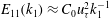
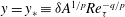
Plots of
 $\overline{u^{\prime 2}}(y)/u_{{\it\tau}}^{2}$
versus
$\overline{u^{\prime 2}}(y)/u_{{\it\tau}}^{2}$
versus
 $y^{+}$
(a) and
$y^{+}$
(a) and
 $y/{\it\delta}$
(b) obtained from the NSTAP Superpipe data of Hultmark et al. (Reference Hultmark, Vallikivi, Bailey and Smits2012, Reference Hultmark, Vallikivi, Bailey and Smits2013) for different values of
$y/{\it\delta}$
(b) obtained from the NSTAP Superpipe data of Hultmark et al. (Reference Hultmark, Vallikivi, Bailey and Smits2012, Reference Hultmark, Vallikivi, Bailey and Smits2013) for different values of
 $\mathit{Re}_{{\it\tau}}$
. The circles are calculated from (4.5) and (4.9) with
$\mathit{Re}_{{\it\tau}}$
. The circles are calculated from (4.5) and (4.9) with
 $C_{0}=1.28$
,
$C_{0}=1.28$
,
 $y_{\ast }={\it\delta}\mathit{Re}_{{\it\tau}}^{-d_{2}/d_{1}}$
for all Reynolds numbers and the values of
$y_{\ast }={\it\delta}\mathit{Re}_{{\it\tau}}^{-d_{2}/d_{1}}$
for all Reynolds numbers and the values of
 $d_{1}$
and
$d_{1}$
and
 $d_{2}$
and the constants in (4.9) given in figure 3.
$d_{2}$
and the constants in (4.9) given in figure 3.

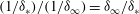
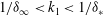
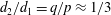
Model parameters
 $C_{s0}$
,
$C_{s0}$
,
 $C_{s1}$
,
$C_{s1}$
,
 $C_{s2}$
,
$C_{s2}$
,
 $d_{1}$
and
$d_{1}$
and
 $d_{2}$
appearing in (4.9). Plotted as functions of
$d_{2}$
appearing in (4.9). Plotted as functions of
 $\mathit{Re}_{{\it\tau}}$
.
$\mathit{Re}_{{\it\tau}}$
.

First note in figure 2 the clear presence when
 $\mathit{Re}_{{\it\tau}}$
is larger than about 20 000 of a logarithmic region at the higher
$\mathit{Re}_{{\it\tau}}$
is larger than about 20 000 of a logarithmic region at the higher
 $y$
-values in agreement with the Townsend–Perry equation (4.5) which fits it quite well (the fit is much better if we allow
$y$
-values in agreement with the Townsend–Perry equation (4.5) which fits it quite well (the fit is much better if we allow
 $C_{\infty }$
to be different from
$C_{\infty }$
to be different from
 $C_{0}$
as in (3.2)). This was of course already noted by Hultmark et al. (Reference Hultmark, Vallikivi, Bailey and Smits2012, Reference Hultmark, Vallikivi, Bailey and Smits2013). Second note the gradual development as
$C_{0}$
as in (3.2)). This was of course already noted by Hultmark et al. (Reference Hultmark, Vallikivi, Bailey and Smits2012, Reference Hultmark, Vallikivi, Bailey and Smits2013). Second note the gradual development as
 $\mathit{Re}_{{\it\tau}}$
increases of a peak of turbulence intensity inside the intermediate region
$\mathit{Re}_{{\it\tau}}$
increases of a peak of turbulence intensity inside the intermediate region
 ${\it\delta}_{{\it\nu}}\ll y\ll {\it\delta}$
. This outer peak is distinct from the well-known near-wall peak at
${\it\delta}_{{\it\nu}}\ll y\ll {\it\delta}$
. This outer peak is distinct from the well-known near-wall peak at
 $y^{+}\approx 15$
and starts appearing clearly at
$y^{+}\approx 15$
and starts appearing clearly at
 $\mathit{Re}_{{\it\tau}}$
larger than about 20 000. Of course this was also noted in Hultmark et al. (Reference Hultmark, Vallikivi, Bailey and Smits2012, Reference Hultmark, Vallikivi, Bailey and Smits2013) who pointed out that the position
$\mathit{Re}_{{\it\tau}}$
larger than about 20 000. Of course this was also noted in Hultmark et al. (Reference Hultmark, Vallikivi, Bailey and Smits2012, Reference Hultmark, Vallikivi, Bailey and Smits2013) who pointed out that the position
 $y_{peak}$
of the outer peak depends on Reynolds number as
$y_{peak}$
of the outer peak depends on Reynolds number as
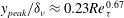 $y_{peak}/{\it\delta}_{{\it\nu}}\approx 0.23\mathit{Re}_{{\it\tau}}^{0.67}$
. In terms of our model this means
$y_{peak}/{\it\delta}_{{\it\nu}}\approx 0.23\mathit{Re}_{{\it\tau}}^{0.67}$
. In terms of our model this means
 $d_{2}/d_{1}=q/p\approx 1/3$
. As predicted by the physics instilled in our model (see the paragraph containing (4.1) and the paragraph preceding it)
$d_{2}/d_{1}=q/p\approx 1/3$
. As predicted by the physics instilled in our model (see the paragraph containing (4.1) and the paragraph preceding it)
 $y_{peak}/{\it\delta}$
decreases and
$y_{peak}/{\it\delta}$
decreases and
 $y_{peak}/{\it\delta}_{{\it\nu}}$
increases with increasing
$y_{peak}/{\it\delta}_{{\it\nu}}$
increases with increasing
 $\mathit{Re}_{{\it\tau}}$
(see figure 2). As also predicted by the physics of our model, the value of
$\mathit{Re}_{{\it\tau}}$
(see figure 2). As also predicted by the physics of our model, the value of
 $\overline{u^{\prime 2}}/u_{{\it\tau}}^{2}$
at the outer peak slowly increases with increasing
$\overline{u^{\prime 2}}/u_{{\it\tau}}^{2}$
at the outer peak slowly increases with increasing
 $\mathit{Re}_{{\it\tau}}$
and the fits in figure 2 which we discuss in the following paragraph indicate that this increase is indeed only logarithmic as in (4.8).
$\mathit{Re}_{{\it\tau}}$
and the fits in figure 2 which we discuss in the following paragraph indicate that this increase is indeed only logarithmic as in (4.8).
The point
 $y=y_{\ast }$
is clearly seen in figure 2 because we did not adopt matching conditions to ensure a continuous passage from (4.9) to (4.5). Nevertheless the new (4.9) returns a satisfactory fit of the outer peak, including its shape, intensity and location. In figure 3 we plot the Reynolds number dependence of the constants
$y=y_{\ast }$
is clearly seen in figure 2 because we did not adopt matching conditions to ensure a continuous passage from (4.9) to (4.5). Nevertheless the new (4.9) returns a satisfactory fit of the outer peak, including its shape, intensity and location. In figure 3 we plot the Reynolds number dependence of the constants
 $C_{s0}$
,
$C_{s0}$
,
 $C_{s1}$
and
$C_{s1}$
and
 $C_{s2}$
,
$C_{s2}$
,
 $d_{1}$
and
$d_{1}$
and
 $d_{2}$
involved in these fits. Note how the parameters
$d_{2}$
involved in these fits. Note how the parameters
 $C_{s1}$
,
$C_{s1}$
,
 $C_{s2}$
,
$C_{s2}$
,
 $d_{1}$
and
$d_{1}$
and
 $d_{2}$
do not deviate much from a constant value except for
$d_{2}$
do not deviate much from a constant value except for
 $C_{s0}$
which grows slowly with
$C_{s0}$
which grows slowly with
 $\mathit{Re}_{{\it\tau}}$
, in fact approximately linearly with
$\mathit{Re}_{{\it\tau}}$
, in fact approximately linearly with
 $\ln \mathit{Re}_{{\it\tau}}$
as in prediction (4.3).
$\ln \mathit{Re}_{{\it\tau}}$
as in prediction (4.3).
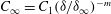
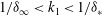
In figure 4 we fit the NSTAP Superpipe data with (4.5) in the range
 $y_{\ast }<y\ll {\it\delta}$
and (4.3) in the range
$y_{\ast }<y\ll {\it\delta}$
and (4.3) in the range
 ${\it\delta}_{{\it\nu}}\ll y<y_{\ast }$
where
${\it\delta}_{{\it\nu}}\ll y<y_{\ast }$
where
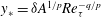 $y_{\ast }={\it\delta}A^{1/p}\mathit{Re}_{{\it\tau}}^{-q/p}$
and with
$y_{\ast }={\it\delta}A^{1/p}\mathit{Re}_{{\it\tau}}^{-q/p}$
and with
 $C_{s0}$
,
$C_{s0}$
,
 $C_{s1}$
and
$C_{s1}$
and
 $C_{s2}$
given by
$C_{s2}$
given by
 $$\begin{eqnarray}\displaystyle & \displaystyle C_{s0}=\frac{C_{0}}{1-m}+C_{0}\ln B+C_{0}{\it\alpha}\frac{q}{p}\ln \mathit{Re}_{{\it\tau}}, & \displaystyle\end{eqnarray}$$
 $$\begin{eqnarray}\displaystyle & C_{s1}=C_{0}({\it\alpha}-1), & \displaystyle\end{eqnarray}$$
 $$\begin{eqnarray}\displaystyle & \displaystyle C_{s2}=\frac{mC_{0}A^{m-1}}{1-m} & \displaystyle\end{eqnarray}$$
 $B=A^{{\it\alpha}/p}$
as obtained above in the text between (4.2) and (4.3). The fits in figure 4 are obtained for
$B=A^{{\it\alpha}/p}$
as obtained above in the text between (4.2) and (4.3). The fits in figure 4 are obtained for
 $A=0.2$
,
$A=0.2$
,
 $C_{0}=1.28$
,
$C_{0}=1.28$
,
 $m=0.37$
,
$m=0.37$
,
 $q=0.79$
,
$q=0.79$
,
 $p=2.38$
and
$p=2.38$
and
 ${\it\alpha}=1.21$
. It works rather well, although not perfectly, for
${\it\alpha}=1.21$
. It works rather well, although not perfectly, for
 $\mathit{Re}_{{\it\tau}}$
larger than about 30 000. Note that we did not optimise the choice of our fitting parameters to obtain the best possible fit. As things stand, (4.9) fits better the outer peak than (4.3) with (4.10)–(4.12) and
$\mathit{Re}_{{\it\tau}}$
larger than about 30 000. Note that we did not optimise the choice of our fitting parameters to obtain the best possible fit. As things stand, (4.9) fits better the outer peak than (4.3) with (4.10)–(4.12) and
 $B=A^{{\it\alpha}/p}$
. However, as of course expected, the latter over-matched model returns a continuous transition to (4.5) at
$B=A^{{\it\alpha}/p}$
. However, as of course expected, the latter over-matched model returns a continuous transition to (4.5) at
 $y=y_{\ast }$
. Note that
$y=y_{\ast }$
. Note that
 $y_{peak}\approx 0.45\,y_{\ast }$
(from
$y_{peak}\approx 0.45\,y_{\ast }$
(from
 $y_{peak}/{\it\delta}_{{\it\nu}}\approx 0.23\,\mathit{Re}_{{\it\tau}}^{0.67}$
and
$y_{peak}/{\it\delta}_{{\it\nu}}\approx 0.23\,\mathit{Re}_{{\it\tau}}^{0.67}$
and
 $y_{\ast }={\it\delta}A^{1/p}\mathit{Re}_{{\it\tau}}^{-q/p}$
).
$y_{\ast }={\it\delta}A^{1/p}\mathit{Re}_{{\it\tau}}^{-q/p}$
).
Plots of
 $\overline{u^{\prime 2}}(y)/u_{{\it\tau}}^{2}$
versus
$\overline{u^{\prime 2}}(y)/u_{{\it\tau}}^{2}$
versus
 $y^{+}$
(a) and
$y^{+}$
(a) and
 $y/{\it\delta}$
(b) obtained from the NSTAP Superpipe data of Hultmark et al. (Reference Hultmark, Vallikivi, Bailey and Smits2012, Reference Hultmark, Vallikivi, Bailey and Smits2013) for different values of
$y/{\it\delta}$
(b) obtained from the NSTAP Superpipe data of Hultmark et al. (Reference Hultmark, Vallikivi, Bailey and Smits2012, Reference Hultmark, Vallikivi, Bailey and Smits2013) for different values of
 $\mathit{Re}_{{\it\tau}}$
. The circles are calculated for all Reynolds numbers from (4.5) and (4.3) with
$\mathit{Re}_{{\it\tau}}$
. The circles are calculated for all Reynolds numbers from (4.5) and (4.3) with
 $y_{\ast }={\it\delta}A^{1/p}\mathit{Re}_{{\it\tau}}^{-q/p}$
and
$y_{\ast }={\it\delta}A^{1/p}\mathit{Re}_{{\it\tau}}^{-q/p}$
and
 $A=0.2$
,
$A=0.2$
,
 $C_{0}=1.28$
,
$C_{0}=1.28$
,
 $m=0.37$
,
$m=0.37$
,
 $q=0.79$
,
$q=0.79$
,
 $p=2.38$
and
$p=2.38$
and
 ${\it\alpha}=1.21$
.
${\it\alpha}=1.21$
.

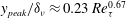
NSTAP Superpipe energy spectra
 $E_{11}(k_{1},y)$
at various distances from the wall for
$E_{11}(k_{1},y)$
at various distances from the wall for
 $\mathit{Re}_{{\it\tau}}=98\,190$
. At this Reynolds number,
$\mathit{Re}_{{\it\tau}}=98\,190$
. At this Reynolds number,
 $y_{\ast }/{\it\delta}_{{\it\nu}}\approx 2130$
. The spectra are normalised by
$y_{\ast }/{\it\delta}_{{\it\nu}}\approx 2130$
. The spectra are normalised by
 $\overline{u^{\prime 2}}(y)L_{11}(y)$
where
$\overline{u^{\prime 2}}(y)L_{11}(y)$
where
 $L_{11}(y)$
are the integral scales obtained from these spectra.
$L_{11}(y)$
are the integral scales obtained from these spectra.

Normalised integral scales
 $L_{11}/{\it\delta}$
obtained from NSTAP Superpipe energy spectra plotted versus
$L_{11}/{\it\delta}$
obtained from NSTAP Superpipe energy spectra plotted versus
 $y/{\it\delta}$
for various Reynolds numbers. Also plotted are the Townsend–Perry and our modified model’s prediction for
$y/{\it\delta}$
for various Reynolds numbers. Also plotted are the Townsend–Perry and our modified model’s prediction for
 $L_{11}/{\it\delta}$
.
$L_{11}/{\it\delta}$
.

Indicatively and only for illustrative purposes, we mention that the fits in figure 4 correspond, approximately (we have rounded off the exponents to make them look like fractions without any intention to suggest a deeper level of theory), to
 ${\it\delta}_{\infty }/{\it\delta}_{\ast }\approx 0.2(y/{\it\delta})^{-7/3}\mathit{Re}_{{\it\tau}}^{-4/5}$
and
${\it\delta}_{\infty }/{\it\delta}_{\ast }\approx 0.2(y/{\it\delta})^{-7/3}\mathit{Re}_{{\it\tau}}^{-4/5}$
and
 ${\it\delta}_{\ast }\approx 2.26{\it\delta}(y/{\it\delta})^{6/5}\mathit{Re}_{{\it\tau}}^{2/5}$
given that
${\it\delta}_{\ast }\approx 2.26{\it\delta}(y/{\it\delta})^{6/5}\mathit{Re}_{{\it\tau}}^{2/5}$
given that
 ${\it\beta}={\it\alpha}q/p$
. The model leading to these particular fits also effectively assumes that the longitudinal spectra in the region
${\it\beta}={\it\alpha}q/p$
. The model leading to these particular fits also effectively assumes that the longitudinal spectra in the region
 ${\it\delta}_{{\it\nu}}\ll y<y_{\ast }\approx 0.5{\it\delta}\mathit{Re}_{{\it\tau}}^{-1/3}$
have a range of wavenumbers
${\it\delta}_{{\it\nu}}\ll y<y_{\ast }\approx 0.5{\it\delta}\mathit{Re}_{{\it\tau}}^{-1/3}$
have a range of wavenumbers
 $1/{\it\delta}_{\infty }<k_{1}<1/{\it\delta}_{\ast }$
which are lower than the usual attached eddy ones and where
$1/{\it\delta}_{\infty }<k_{1}<1/{\it\delta}_{\ast }$
which are lower than the usual attached eddy ones and where
 $E_{11}(k_{1})\approx (2/3)u_{{\it\tau}}^{2}y\mathit{Re}_{{\it\tau}}^{1/3}(k_{1}{\it\delta})^{-1/3}=(2/3)u_{{\it\tau}}^{2}y(k_{1}{\it\delta}_{{\it\nu}})^{-1/3}$
. Note the presence of both
$E_{11}(k_{1})\approx (2/3)u_{{\it\tau}}^{2}y\mathit{Re}_{{\it\tau}}^{1/3}(k_{1}{\it\delta})^{-1/3}=(2/3)u_{{\it\tau}}^{2}y(k_{1}{\it\delta}_{{\it\nu}})^{-1/3}$
. Note the presence of both
 $y$
and
$y$
and
 ${\it\delta}_{{\it\nu}}$
in these particularly low-wavenumber spectra. Note also that
${\it\delta}_{{\it\nu}}$
in these particularly low-wavenumber spectra. Note also that
 ${\it\delta}_{\ast }<0.2{\it\delta}$
and
${\it\delta}_{\ast }<0.2{\it\delta}$
and
 ${\it\delta}_{\infty }>5{\it\delta}/100$
given that
${\it\delta}_{\infty }>5{\it\delta}/100$
given that
 $y<y_{\ast }\approx 0.5{\it\delta}\mathit{Re}_{{\it\tau}}^{-1/3}$
. Finally,
$y<y_{\ast }\approx 0.5{\it\delta}\mathit{Re}_{{\it\tau}}^{-1/3}$
. Finally,
 $y_{\ast }>15{\it\delta}_{{\it\nu}}$
as long as
$y_{\ast }>15{\it\delta}_{{\it\nu}}$
as long as
 $\mathit{Re}_{{\it\tau}}>165$
.
$\mathit{Re}_{{\it\tau}}>165$
.
In the region
 $y_{\ast }\approx 0.5{\it\delta}\mathit{Re}_{{\it\tau}}^{-1/3}<y\ll {\it\delta}$
no such spectral range exists; only the attached eddy form
$y_{\ast }\approx 0.5{\it\delta}\mathit{Re}_{{\it\tau}}^{-1/3}<y\ll {\it\delta}$
no such spectral range exists; only the attached eddy form
 $E_{11}\approx 1.28u_{{\it\tau}}^{2}k_{1}^{-1}$
is present in the usual range
$E_{11}\approx 1.28u_{{\it\tau}}^{2}k_{1}^{-1}$
is present in the usual range
 $1/{\it\delta}<k_{1}<1/y$
. The constant
$1/{\it\delta}<k_{1}<1/y$
. The constant
 $C_{0}=1.28$
is the one used to fit the data in both figures 4 and 2.
$C_{0}=1.28$
is the one used to fit the data in both figures 4 and 2.
Figure 5 shows spectra plotted indicatively as wavenumber spectra at many distances from the wall for a value of
 $\mathit{Re}_{{\it\tau}}$
equal to 98 190 and
$\mathit{Re}_{{\it\tau}}$
equal to 98 190 and
 $y_{\ast }/{\it\delta}_{{\it\nu}}\approx 2130$
. These spectra are really frequency spectra as we cannot expect the Taylor hypothesis to be accurate enough at the lower wavenumbers and at the closer positions to the wall. With this serious caveat firmly in mind it is nevertheless intriguing to see in figure 5 that very high-Reynolds-number spectra do indeed have an extra low-frequency range at
$y_{\ast }/{\it\delta}_{{\it\nu}}\approx 2130$
. These spectra are really frequency spectra as we cannot expect the Taylor hypothesis to be accurate enough at the lower wavenumbers and at the closer positions to the wall. With this serious caveat firmly in mind it is nevertheless intriguing to see in figure 5 that very high-Reynolds-number spectra do indeed have an extra low-frequency range at
 $y<y_{\ast }$
where the spectrum is much shallower than
$y<y_{\ast }$
where the spectrum is much shallower than
 $k_{1}^{-1}$
yet not constant; and that this range is absent at higher positions from the wall where
$k_{1}^{-1}$
yet not constant; and that this range is absent at higher positions from the wall where
 $y>y_{\ast }$
. At distances
$y>y_{\ast }$
. At distances
 $y$
from the wall larger than
$y$
from the wall larger than
 $y_{\ast }$
one sees a spectral wavenumber dependence which is close to
$y_{\ast }$
one sees a spectral wavenumber dependence which is close to
 $k_{1}^{-1}$
(perhaps a little steeper) between a very low-wavenumber constant spectrum and a very high-wavenumber spectrum which is much steeper than
$k_{1}^{-1}$
(perhaps a little steeper) between a very low-wavenumber constant spectrum and a very high-wavenumber spectrum which is much steeper than
 $k_{1}^{-1}$
, perhaps close to
$k_{1}^{-1}$
, perhaps close to
 $k_{1}^{-5/3}$
. Even the deviation from the
$k_{1}^{-5/3}$
. Even the deviation from the
 $k_{1}^{-1}$
spectrum which makes it look a little steeper could be a frequency domain signature which does not quite correspond to
$k_{1}^{-1}$
spectrum which makes it look a little steeper could be a frequency domain signature which does not quite correspond to
 $k_{1}^{-1}$
because of Taylor hypothesis failure, see del Alamo & Jimenez (Reference del Alamo and Jimenez2009) but also Rosenberg et al. (Reference Rosenberg, Hultmark, Vallikivi, Bailey and Smits2013).
$k_{1}^{-1}$
because of Taylor hypothesis failure, see del Alamo & Jimenez (Reference del Alamo and Jimenez2009) but also Rosenberg et al. (Reference Rosenberg, Hultmark, Vallikivi, Bailey and Smits2013).
Our initial motivation for modifying the Perry et al. (Reference Perry, Henbest and Chong1986) model and adding an extra spectral range to it was the
 $y$
-dependence of the integral scale. The values of the exponents
$y$
-dependence of the integral scale. The values of the exponents
 ${\it\alpha}$
,
${\it\alpha}$
,
 $q$
,
$q$
,
 $p$
and
$p$
and
 $m$
used in the fits of figure 4 combined with the constraint
$m$
used in the fits of figure 4 combined with the constraint
 ${\it\beta}={\it\alpha}q/p$
are such that
${\it\beta}={\it\alpha}q/p$
are such that
 $L_{11}/{\it\delta}\sim (y/{\it\delta})^{1/3}\mathit{Re}_{{\it\tau}}^{0.1}$
if we neglect the logarithmic dependence of
$L_{11}/{\it\delta}\sim (y/{\it\delta})^{1/3}\mathit{Re}_{{\it\tau}}^{0.1}$
if we neglect the logarithmic dependence of
 $\overline{u^{\prime 2}}(y)/u_{{\it\tau}}^{2}$
in (4.4). In figure 6 we plot
$\overline{u^{\prime 2}}(y)/u_{{\it\tau}}^{2}$
in (4.4). In figure 6 we plot
 $L_{11}/{\it\delta}$
versus
$L_{11}/{\it\delta}$
versus
 $y/{\it\delta}$
as obtained from the lowest frequencies of the NSTAP Superpipe spectra (see for example figure 5) for different Reynolds numbers. Again, the integral scales plotted in figure 6 should be taken with much caution and only very indicatively as they are really integral time scales and the Taylor hypothesis cannot be invoked at these low frequencies. In that same figure we nevertheless plot the Townsend–Perry formula (3.3) where
$y/{\it\delta}$
as obtained from the lowest frequencies of the NSTAP Superpipe spectra (see for example figure 5) for different Reynolds numbers. Again, the integral scales plotted in figure 6 should be taken with much caution and only very indicatively as they are really integral time scales and the Taylor hypothesis cannot be invoked at these low frequencies. In that same figure we nevertheless plot the Townsend–Perry formula (3.3) where
 $C_{\infty }=C_{0}$
as per the fitting constants for figure 4 (i.e.
$C_{\infty }=C_{0}$
as per the fitting constants for figure 4 (i.e.
 $L_{11}\approx {\rm\pi}{\it\delta}/(1+\ln ({\it\delta}/y))$
) and formula (4.4). In (4.4) we used the fitting constants that we also used for the fits in figure 4. Note that (4.4) is defined for
$L_{11}\approx {\rm\pi}{\it\delta}/(1+\ln ({\it\delta}/y))$
) and formula (4.4). In (4.4) we used the fitting constants that we also used for the fits in figure 4. Note that (4.4) is defined for
 $y$
in the range
$y$
in the range
 ${\it\delta}_{{\it\nu}}\ll y<y_{\ast }=0.5{\it\delta}\mathit{Re}_{{\it\tau}}^{-1/3}$
and that, even in the modified model,
${\it\delta}_{{\it\nu}}\ll y<y_{\ast }=0.5{\it\delta}\mathit{Re}_{{\it\tau}}^{-1/3}$
and that, even in the modified model,
 $L_{11}$
is given by (3.3) in the range
$L_{11}$
is given by (3.3) in the range
 $y_{\ast }\ll y<{\it\delta}$
. The points in figure 6 where the modified model curves meet the Townsend–Perry curve are at
$y_{\ast }\ll y<{\it\delta}$
. The points in figure 6 where the modified model curves meet the Townsend–Perry curve are at
 $y=y_{\ast }$
for the different
$y=y_{\ast }$
for the different
 $\mathit{Re}_{{\it\tau}}$
. It is clear that the modified model succeeds in steepening the
$\mathit{Re}_{{\it\tau}}$
. It is clear that the modified model succeeds in steepening the
 $y$
-dependence of
$y$
-dependence of
 $L_{11}$
in the range
$L_{11}$
in the range
 ${\it\delta}_{{\it\nu}}\ll y<y_{\ast }$
and that it keeps the original
${\it\delta}_{{\it\nu}}\ll y<y_{\ast }$
and that it keeps the original
 $y$
-dependence of
$y$
-dependence of
 $L_{11}$
in the range
$L_{11}$
in the range
 $y_{\ast }\ll y<{\it\delta}$
. It is also clear, though, that formulae (4.4) and (3.3) do not match the NSTAP Superpipe integral scales well with the fitting constants used for figure 4. We repeat that the integral scales obtained from the NSTAP Superpipe data are really integral time scales and it is not clear that they should be proportional to
$y_{\ast }\ll y<{\it\delta}$
. It is also clear, though, that formulae (4.4) and (3.3) do not match the NSTAP Superpipe integral scales well with the fitting constants used for figure 4. We repeat that the integral scales obtained from the NSTAP Superpipe data are really integral time scales and it is not clear that they should be proportional to
 $L_{11}$
. If such a proportionality could be established, however, then the data would indicate that
$L_{11}$
. If such a proportionality could be established, however, then the data would indicate that
 $L_{11}/{\it\delta}\sim (y/{\it\delta})^{1/3}$
for all Reynolds numbers in some agreement with our modified model’s
$L_{11}/{\it\delta}\sim (y/{\it\delta})^{1/3}$
for all Reynolds numbers in some agreement with our modified model’s
 $L_{11}/{\it\delta}\sim (y/{\it\delta})^{1/3}\mathit{Re}_{{\it\tau}}^{0.1}$
, but the constants of proportionality are different.
$L_{11}/{\it\delta}\sim (y/{\it\delta})^{1/3}\mathit{Re}_{{\it\tau}}^{0.1}$
, but the constants of proportionality are different.
Finally, we draw attention to the fact that the integral scale
 $L_{11}$
is not proportional to
$L_{11}$
is not proportional to
 $y$
in the range
$y$
in the range
 ${\it\delta}_{{\it\nu}}\ll y\ll {\it\delta}$
as one might have expected (see Tomkins & Adrian Reference Tomkins and Adrian2003 who found several spanwise length scales, including
${\it\delta}_{{\it\nu}}\ll y\ll {\it\delta}$
as one might have expected (see Tomkins & Adrian Reference Tomkins and Adrian2003 who found several spanwise length scales, including
 $L_{11}$
, to be proportional to
$L_{11}$
, to be proportional to
 $y$
in a turbulent boundary layer).
$y$
in a turbulent boundary layer).
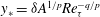
5. Intermittent attached eddies
We now address the possibility brought up by experimental results such as figure 5 that, in the appropriate Townsend–Perry attached eddy range of wavenumbers, the energy spectra may not scale as
 $k_{1}^{-1}$
but as a slightly steeper power of
$k_{1}^{-1}$
but as a slightly steeper power of
 $k_{1}$
. As pointed out by del Alamo & Jimenez (Reference del Alamo and Jimenez2009), observed deviations from
$k_{1}$
. As pointed out by del Alamo & Jimenez (Reference del Alamo and Jimenez2009), observed deviations from
 $k_{1}^{-1}$
could result from a failure of the Taylor hypothesis, a point which we do not dispute. However, we show in this section that slightly steeper powers of
$k_{1}^{-1}$
could result from a failure of the Taylor hypothesis, a point which we do not dispute. However, we show in this section that slightly steeper powers of
 $k_{1}$
can also arise because of intermittent fluctuations of the wall shear stress, as observed for example by Alfredsson et al. (Reference Alfredsson, Johansson, Haritonidis and Eckelmann1988) and Örlü & Schlatter (Reference Örlü and Schlatter2011).
$k_{1}$
can also arise because of intermittent fluctuations of the wall shear stress, as observed for example by Alfredsson et al. (Reference Alfredsson, Johansson, Haritonidis and Eckelmann1988) and Örlü & Schlatter (Reference Örlü and Schlatter2011).
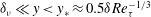
One way to argue, in the region
 ${\it\delta}_{{\it\nu}}\ll y\ll {\it\delta}$
, that
${\it\delta}_{{\it\nu}}\ll y\ll {\it\delta}$
, that
 $E_{11}(k_{1},y)\sim u_{{\it\tau}}^{2}k_{1}^{-1}$
in the wavenumber range
$E_{11}(k_{1},y)\sim u_{{\it\tau}}^{2}k_{1}^{-1}$
in the wavenumber range
 $1/{\it\delta}\ll y\ll 1/y$
is by hypothesising that the attached eddies dominate the spectrum in that range independently of
$1/{\it\delta}\ll y\ll 1/y$
is by hypothesising that the attached eddies dominate the spectrum in that range independently of
 $y$
and that these eddies are themselves dominated by the wall shear stress, i.e. the skin friction, at the wall. Hence,
$y$
and that these eddies are themselves dominated by the wall shear stress, i.e. the skin friction, at the wall. Hence,
 $E_{11}(k_{1},y)$
can only depend on
$E_{11}(k_{1},y)$
can only depend on
 $u_{{\it\tau}}^{2}$
and
$u_{{\it\tau}}^{2}$
and
 $k_{1}$
in the region
$k_{1}$
in the region
 ${\it\delta}_{{\it\nu}}\ll y\ll {\it\delta}$
, which implies that
${\it\delta}_{{\it\nu}}\ll y\ll {\it\delta}$
, which implies that
 $E_{11}(k_{1},y)\sim u_{{\it\tau}}^{2}k_{1}^{-1}$
.
$E_{11}(k_{1},y)\sim u_{{\it\tau}}^{2}k_{1}^{-1}$
.
We now show how this argument can be modified to take into account the intermittency in the wall shear stress. To do this we adopt the way that Kolmogorov (Reference Kolmogorov1962) took into account the inertial-range intermittency of kinetic energy dissipation in homogeneous turbulence and adapt it to the intermittency of wall shear stress in wall turbulence. We therefore define the scale-dependent filter averages
 $$\begin{eqnarray}u_{\ast }^{2}(x,r,t)=\frac{1}{2r}\int _{x-r}^{x+r}{\it\nu}\left.\frac{\text{d}u}{\text{d}y}\right|_{wall}(x,t)\,\text{d}x.\end{eqnarray}$$
Following Kolmogorov’s (Reference Kolmogorov1962) approach we assume that the statistics of
 $u_{\ast }^{2}(x,r,t)$
are lognormal at scales
$u_{\ast }^{2}(x,r,t)$
are lognormal at scales
 $r$
large enough for
$r$
large enough for
 $u_{\ast }^{2}(x,r,t)$
to be reasonably presumed positive. It may be reasonable to assume scales
$u_{\ast }^{2}(x,r,t)$
to be reasonably presumed positive. It may be reasonable to assume scales
 $r$
much larger than
$r$
much larger than
 $y$
to be such scales if
$y$
to be such scales if
 ${\it\delta}_{{\it\nu}}\ll y\ll {\it\delta}$
. For such scales we therefore define
${\it\delta}_{{\it\nu}}\ll y\ll {\it\delta}$
. For such scales we therefore define
 ${\it\xi}_{r}\equiv \ln (u_{\ast }^{2}/u_{{\it\tau}}^{2})$
and assume
${\it\xi}_{r}\equiv \ln (u_{\ast }^{2}/u_{{\it\tau}}^{2})$
and assume
 ${\it\xi}_{r}$
to be a Gaussian-distributed random variable, i.e. its probability distribution function (PDF) is
${\it\xi}_{r}$
to be a Gaussian-distributed random variable, i.e. its probability distribution function (PDF) is
 $$\begin{eqnarray}P({\it\xi}_{r})=\frac{1}{\sqrt{2{\rm\pi}}{\it\sigma}_{r}}\text{e}^{-({\it\xi}_{r}-m_{r})^{2}/2{\it\sigma}_{r}^{2}}.\end{eqnarray}$$
The constraint
 $\langle u_{\ast }^{2}(x,r,t)\rangle =u_{{\it\tau}}^{2}$
implies
$\langle u_{\ast }^{2}(x,r,t)\rangle =u_{{\it\tau}}^{2}$
implies
 $m_{r}=-{\it\sigma}_{r}^{2}/2$
(the angular brackets signify an average over time or over
$m_{r}=-{\it\sigma}_{r}^{2}/2$
(the angular brackets signify an average over time or over
 $x$
or both). The exact form of this PDF does not really matter as we are only concerned with low-order moments.
$x$
or both). The exact form of this PDF does not really matter as we are only concerned with low-order moments.
We now hypothesise that, in the appropriate Townsend–Perry attached eddy range of wavenumbers, the average of
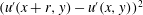 $(u^{\prime }(x+r,y)-u^{\prime }(x,y))^{2}$
conditioned on a given value of
$(u^{\prime }(x+r,y)-u^{\prime }(x,y))^{2}$
conditioned on a given value of
 $u_{\ast }^{2}(x,r,t)$
depends only on that value and
$u_{\ast }^{2}(x,r,t)$
depends only on that value and
 $r$
(
$r$
(
 $u^{\prime }$
is the streamwise fluctuating turbulence velocity component). By dimensional analysis the dependence on
$u^{\prime }$
is the streamwise fluctuating turbulence velocity component). By dimensional analysis the dependence on
 $r$
drops out, and as the structure function
$r$
drops out, and as the structure function
 $\langle (u^{\prime }(x+r,y)-u^{\prime }(x,y))^{2}\rangle$
is the average over all of these conditional averages, we are left with
$\langle (u^{\prime }(x+r,y)-u^{\prime }(x,y))^{2}\rangle$
is the average over all of these conditional averages, we are left with
 $\langle (u^{\prime }(x+r,y)-u^{\prime }(x,y))^{2}\rangle \sim \langle u_{\ast }^{2}(x,r,t)\rangle$
. Using (5.2) to calculate this average, we obtain
$\langle (u^{\prime }(x+r,y)-u^{\prime }(x,y))^{2}\rangle \sim \langle u_{\ast }^{2}(x,r,t)\rangle$
. Using (5.2) to calculate this average, we obtain
 $$\begin{eqnarray}\langle (u^{\prime }(x+r,y)-u^{\prime }(x,y))^{2}\rangle \sim u_{{\it\tau}}^{2}\int \text{d}{\it\xi}\,\frac{\text{e}^{{\it\xi}}}{\sqrt{2{\rm\pi}}{\it\sigma}_{r}}\text{e}^{-({\it\xi}-m_{r})^{2}/2{\it\sigma}_{r}^{2}}\sim u_{{\it\tau}}^{2}\text{e}^{-{\it\sigma}_{r}^{2}/9}.\end{eqnarray}$$
A logarithmic dependence of
 ${\it\sigma}_{r}^{2}$
on
${\it\sigma}_{r}^{2}$
on
 $r$
, for example
$r$
, for example
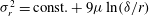 ${\it\sigma}_{r}^{2}=\text{const.}+9{\it\mu}\ln ({\it\delta}/r)$
where
${\it\sigma}_{r}^{2}=\text{const.}+9{\it\mu}\ln ({\it\delta}/r)$
where
 ${\it\mu}>0$
, returns
${\it\mu}>0$
, returns
 $\langle (u^{\prime }(x+r,y)-u^{\prime }(x,y))^{2}\rangle \sim u_{{\it\tau}}^{2}(r/{\it\delta})^{{\it\mu}}$
, i.e.
$\langle (u^{\prime }(x+r,y)-u^{\prime }(x,y))^{2}\rangle \sim u_{{\it\tau}}^{2}(r/{\it\delta})^{{\it\mu}}$
, i.e.
 $$\begin{eqnarray}E_{11}(k_{1},y)\sim u_{{\it\tau}}^{2}{\it\delta}(k_{1}{\it\delta})^{-1-{\it\mu}}.\end{eqnarray}$$
This demonstrates that the attached eddy hypothesis suitably modified to take into account the intermittent fluctuations of the wall shear stress can lead to spectra that are slightly steeper than
 $k_{1}^{-1}$
. The statistics of the intermittently fluctuating wall shear stress can therefore have some bearing on energy spectra and, in turn, on vertical profiles of the turbulent kinetic energy. One can readily see that replacement of
$k_{1}^{-1}$
. The statistics of the intermittently fluctuating wall shear stress can therefore have some bearing on energy spectra and, in turn, on vertical profiles of the turbulent kinetic energy. One can readily see that replacement of
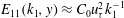 $E_{11}(k_{1},y)\approx C_{0}u_{{\it\tau}}^{2}k_{1}^{-1}$
by
$E_{11}(k_{1},y)\approx C_{0}u_{{\it\tau}}^{2}k_{1}^{-1}$
by
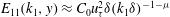 $E_{11}(k_{1},y)\approx C_{0}u_{{\it\tau}}^{2}{\it\delta}(k_{1}{\it\delta})^{-1-{\it\mu}}$
in range (ii) of the Perry et al. (Reference Perry, Henbest and Chong1986) model (§ 3) and in range (iii) of our modified model (§ 4) would lead to profiles such as (4.5) and (4.9) where the
$E_{11}(k_{1},y)\approx C_{0}u_{{\it\tau}}^{2}{\it\delta}(k_{1}{\it\delta})^{-1-{\it\mu}}$
in range (ii) of the Perry et al. (Reference Perry, Henbest and Chong1986) model (§ 3) and in range (iii) of our modified model (§ 4) would lead to profiles such as (4.5) and (4.9) where the
 $\ln ({\it\delta}/y)$
terms would be replaced by weak power laws of
$\ln ({\it\delta}/y)$
terms would be replaced by weak power laws of
 $y/{\it\delta}$
. However, for very small exponents
$y/{\it\delta}$
. However, for very small exponents
 ${\it\mu}$
this difference would be very hard to detect experimentally.
${\it\mu}$
this difference would be very hard to detect experimentally.
6. The mean flow profile
As already noted by Townsend (Reference Townsend1976), the attached eddy hypothesis is incompatible with the assumption that
 $\text{d}\overline{u}/\text{d}y$
is independent of
$\text{d}\overline{u}/\text{d}y$
is independent of
 ${\it\delta}$
. This assumption is required to argue that
${\it\delta}$
. This assumption is required to argue that
 $\text{d}\overline{u}/\text{d}y$
depends only on
$\text{d}\overline{u}/\text{d}y$
depends only on
 $y$
and
$y$
and
 $u_{{\it\tau}}$
in the range
$u_{{\it\tau}}$
in the range
 ${\it\delta}_{{\it\nu}}\ll y\ll {\it\delta}$
. As
${\it\delta}_{{\it\nu}}\ll y\ll {\it\delta}$
. As
 $\mathit{Re}_{{\it\tau}}\rightarrow \infty$
an intermediate layer
$\mathit{Re}_{{\it\tau}}\rightarrow \infty$
an intermediate layer
 ${\it\delta}_{{\it\nu}}\ll y\ll {\it\delta}$
does emerge, however, where something may nevertheless be independent of
${\it\delta}_{{\it\nu}}\ll y\ll {\it\delta}$
does emerge, however, where something may nevertheless be independent of
 ${\it\nu}$
and
${\it\nu}$
and
 ${\it\delta}$
. Dallas et al. (Reference Dallas, Vassilicos and Hewitt2009) presented evidence from direct numerical simulations (DNS) of turbulent channel flow which shows that the eddy turnover time
${\it\delta}$
. Dallas et al. (Reference Dallas, Vassilicos and Hewitt2009) presented evidence from direct numerical simulations (DNS) of turbulent channel flow which shows that the eddy turnover time
 ${\it\tau}\equiv E/{\it\epsilon}$
(where
${\it\tau}\equiv E/{\it\epsilon}$
(where
 $E$
is the total turbulent kinetic energy) is proportional to
$E$
is the total turbulent kinetic energy) is proportional to
 $y/u_{{\it\tau}}$
in the range
$y/u_{{\it\tau}}$
in the range
 ${\it\delta}_{{\it\nu}}\ll y\ll {\it\delta}$
for a variety of moderate values of
${\it\delta}_{{\it\nu}}\ll y\ll {\it\delta}$
for a variety of moderate values of
 $\mathit{Re}_{{\it\tau}}$
.
$\mathit{Re}_{{\it\tau}}$
.
Here we make the reasonable extrapolation that the observation of Dallas et al. (Reference Dallas, Vassilicos and Hewitt2009) is not limited to moderate Reynolds numbers and that
 ${\it\tau}$
is independent of
${\it\tau}$
is independent of
 ${\it\nu}$
and
${\it\nu}$
and
 ${\it\delta}$
at all large enough Reynolds numbers. Hence,
${\it\delta}$
at all large enough Reynolds numbers. Hence,
 ${\it\tau}\sim y/u_{{\it\tau}}$
in the range
${\it\tau}\sim y/u_{{\it\tau}}$
in the range
 ${\it\delta}_{{\it\nu}}\ll y\ll {\it\delta}$
for turbulent pipe flows.
${\it\delta}_{{\it\nu}}\ll y\ll {\it\delta}$
for turbulent pipe flows.
Following Townsend (Reference Townsend1976) we also assume local balance between production and dissipation, i.e.
 $-\langle u^{\prime }v^{\prime }\rangle (\text{d}\overline{u}/\text{d}y)\approx {\it\epsilon}=E/{\it\tau}$
, but only in a region
$-\langle u^{\prime }v^{\prime }\rangle (\text{d}\overline{u}/\text{d}y)\approx {\it\epsilon}=E/{\it\tau}$
, but only in a region
 $y_{P{\it\epsilon}}<y\ll {\it\delta}$
where
$y_{P{\it\epsilon}}<y\ll {\it\delta}$
where
 ${\it\delta}_{{\it\nu}}\ll y_{P{\it\epsilon}}$
. Making use of the well-known axial momentum balance in turbulent pipe flow, see Pope (Reference Pope2000),
${\it\delta}_{{\it\nu}}\ll y_{P{\it\epsilon}}$
. Making use of the well-known axial momentum balance in turbulent pipe flow, see Pope (Reference Pope2000),
 $$\begin{eqnarray}{\it\nu}\frac{\text{d}}{\text{d}y}\overline{u}-\langle u^{\prime }v^{\prime }\rangle =u_{{\it\tau}}^{2}(1-y/{\it\delta}),\end{eqnarray}$$
and introducing the constant
 $C_{s}$
in
$C_{s}$
in
 ${\it\tau}\approx C_{s}(y/u_{{\it\tau}})$
, we are led to
${\it\tau}\approx C_{s}(y/u_{{\it\tau}})$
, we are led to
 $$\begin{eqnarray}\left(1-y/{\it\delta}-\frac{\text{d}\overline{u}_{+}}{\text{d}y^{+}}\right)\frac{\text{d}\overline{u}_{+}}{\text{d}\ln y^{+}}\approx C_{s}E/u_{{\it\tau}}^{2}=C_{s}E^{+}\end{eqnarray}$$
in the region
 $y_{P{\it\epsilon}}<y\ll {\it\delta}$
.
$y_{P{\it\epsilon}}<y\ll {\it\delta}$
.
We know from the Townsend–Perry attached eddy model and also from this paper’s modified model that
 $E^{+}\approx M_{0}+M_{1}\ln ({\it\delta}/y)$
in the range
$E^{+}\approx M_{0}+M_{1}\ln ({\it\delta}/y)$
in the range
 $y_{\ast }<y\ll {\it\delta}$
where
$y_{\ast }<y\ll {\it\delta}$
where
 $M_{0}$
and
$M_{0}$
and
 $M_{1}$
are constants different from
$M_{1}$
are constants different from
 $C_{\infty }$
and
$C_{\infty }$
and
 $C_{0}$
in (3.2) because one needs to also take into account
$C_{0}$
in (3.2) because one needs to also take into account
 $(\overline{w^{\prime 2}}(y)/2)/u_{{\it\tau}}^{2}$
and
$(\overline{w^{\prime 2}}(y)/2)/u_{{\it\tau}}^{2}$
and
 $(\overline{v^{\prime 2}}(y)/2)/u_{{\it\tau}}^{2}$
. Hence, the first prediction of our approach based on
$(\overline{v^{\prime 2}}(y)/2)/u_{{\it\tau}}^{2}$
. Hence, the first prediction of our approach based on
 ${\it\tau}\approx C_{s}(y/u_{{\it\tau}})$
and
${\it\tau}\approx C_{s}(y/u_{{\it\tau}})$
and
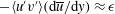 $-\langle u^{\prime }v^{\prime }\rangle (\text{d}\overline{u}/\text{d}y)\approx {\it\epsilon}$
is that the left-hand side of (6.2) is approximately equal to
$-\langle u^{\prime }v^{\prime }\rangle (\text{d}\overline{u}/\text{d}y)\approx {\it\epsilon}$
is that the left-hand side of (6.2) is approximately equal to
 $C_{s}M_{0}+C_{s}M_{1}\ln ({\it\delta}/y)$
in
$C_{s}M_{0}+C_{s}M_{1}\ln ({\it\delta}/y)$
in
 $y_{\ast }<y\ll {\it\delta}$
.
$y_{\ast }<y\ll {\it\delta}$
.
If
 $E^{+}$
has an outer peak at the same
$E^{+}$
has an outer peak at the same
 $y=y_{peak}$
location as
$y=y_{peak}$
location as
 $(\overline{u^{\prime 2}}(y)/2)/u_{{\it\tau}}^{2}$
and if
$(\overline{u^{\prime 2}}(y)/2)/u_{{\it\tau}}^{2}$
and if
 $y_{P{\it\epsilon}}<y_{peak}$
then the second prediction of our approach is that the left-hand side of (6.2) has an outer peak at
$y_{P{\it\epsilon}}<y_{peak}$
then the second prediction of our approach is that the left-hand side of (6.2) has an outer peak at
 $y=y_{peak}$
.
$y=y_{peak}$
.
Figure 7 is a plot of the left-hand side of (6.2) based on the NSTAP Superpipe data of Hultmark et al. (Reference Hultmark, Vallikivi, Bailey and Smits2012, Reference Hultmark, Vallikivi, Bailey and Smits2013). This plot suggests that there is indeed an outer peak in the functional dependence on
 $y$
of the left-hand side of (6.2). It is also not inconsistent with the prediction that the left-hand side of (6.2) is a logarithmically decreasing function of
$y$
of the left-hand side of (6.2). It is also not inconsistent with the prediction that the left-hand side of (6.2) is a logarithmically decreasing function of
 $y$
for much of the region where
$y$
for much of the region where
 $y$
is greater than the location of this outer peak. Figure 8 shows this left-hand side for the higher
$y$
is greater than the location of this outer peak. Figure 8 shows this left-hand side for the higher
 $\mathit{Re}_{{\it\tau}}$
NSTAP Superpipe data (
$\mathit{Re}_{{\it\tau}}$
NSTAP Superpipe data (
 $\mathit{Re}_{{\it\tau}}$
between 20 000 and 100 000). There is no evidence that the left-hand side of (6.2) decreases logarithmically with
$\mathit{Re}_{{\it\tau}}$
between 20 000 and 100 000). There is no evidence that the left-hand side of (6.2) decreases logarithmically with
 $y$
for the lower Reynolds numbers in figure 7, in agreement with (6.2) and figures 2 and 4 which show that there is no such logarithmic decrease in
$y$
for the lower Reynolds numbers in figure 7, in agreement with (6.2) and figures 2 and 4 which show that there is no such logarithmic decrease in
 $(\overline{u^{\prime 2}}(y)/2)/u_{{\it\tau}}^{2}$
either at
$(\overline{u^{\prime 2}}(y)/2)/u_{{\it\tau}}^{2}$
either at
 $\mathit{Re}_{{\it\tau}}<10\,000$
. However, such a
$\mathit{Re}_{{\it\tau}}<10\,000$
. However, such a
 $y$
-dependence is not inconsistent with much of the
$y$
-dependence is not inconsistent with much of the
 $y$
-dependence for the
$y$
-dependence for the
 $\mathit{Re}_{{\it\tau}}>20\,000$
data at the right of the outer peak in figure 8.
$\mathit{Re}_{{\it\tau}}>20\,000$
data at the right of the outer peak in figure 8.
Linear-logarithmic plot of
 $(1-y/{\it\delta}-(\text{d}\overline{u}_{+}/\text{d}y^{+}))(\text{d}\overline{u}_{+}/\text{d}\ln y^{+})$
versus
$(1-y/{\it\delta}-(\text{d}\overline{u}_{+}/\text{d}y^{+}))(\text{d}\overline{u}_{+}/\text{d}\ln y^{+})$
versus
 $y^{+}$
for different values of
$y^{+}$
for different values of
 $\mathit{Re}_{{\it\tau}}$
obtained from the NSTAP Superpipe mean flow data of Hultmark et al. (Reference Hultmark, Vallikivi, Bailey and Smits2012, Reference Hultmark, Vallikivi, Bailey and Smits2013).
$\mathit{Re}_{{\it\tau}}$
obtained from the NSTAP Superpipe mean flow data of Hultmark et al. (Reference Hultmark, Vallikivi, Bailey and Smits2012, Reference Hultmark, Vallikivi, Bailey and Smits2013).

Blow up of figure 7 for the four highest Reynolds numbers with a superposed dotted line suggesting logarithmic dependence of
 $(1-y/{\it\delta}-(\text{d}\overline{u}_{+}/\text{d}y^{+}))(\text{d}\overline{u}_{+}/\text{d}\ln y^{+})$
on
$(1-y/{\it\delta}-(\text{d}\overline{u}_{+}/\text{d}y^{+}))(\text{d}\overline{u}_{+}/\text{d}\ln y^{+})$
on
 $y$
at the right of the peak.
$y$
at the right of the peak.

In figure 9 we replot the high-
 $\mathit{Re}_{{\it\tau}}$
data of figure 8 but as functions of
$\mathit{Re}_{{\it\tau}}$
data of figure 8 but as functions of
 $y/{\it\delta}$
in one plot and of
$y/{\it\delta}$
in one plot and of
 $y/y_{peak}$
in the other. These plots demonstrate that the position of the outer peak in the left-hand side of (6.2) is the same as the position of the outer peak in
$y/y_{peak}$
in the other. These plots demonstrate that the position of the outer peak in the left-hand side of (6.2) is the same as the position of the outer peak in
 $(\overline{u^{\prime 2}}(y)/2)/u_{{\it\tau}}^{2}$
. And they also demonstrate that the left-hand side of (6.2), if indeed logarithmically decreasing, is approximately equal to
$(\overline{u^{\prime 2}}(y)/2)/u_{{\it\tau}}^{2}$
. And they also demonstrate that the left-hand side of (6.2), if indeed logarithmically decreasing, is approximately equal to
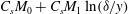 $C_{s}M_{0}+C_{s}M_{1}\ln ({\it\delta}/y)$
in
$C_{s}M_{0}+C_{s}M_{1}\ln ({\it\delta}/y)$
in
 $y_{\ast }<y\ll {\it\delta}$
(though the data in our disposal do not permit us to check that the constants
$y_{\ast }<y\ll {\it\delta}$
(though the data in our disposal do not permit us to check that the constants
 $C_{s}M_{0}$
and
$C_{s}M_{0}$
and
 $C_{s}M_{1}$
are indeed the products of
$C_{s}M_{1}$
are indeed the products of
 $C_{s}$
with
$C_{s}$
with
 $M_{0}$
and
$M_{0}$
and
 $M_{1}$
respectively).
$M_{1}$
respectively).
Blow ups of figure 7 for the four highest Reynolds numbers plotted versus
 $y/{\it\delta}$
(a) and versus
$y/{\it\delta}$
(a) and versus
 $y/y_{peak}$
(b) where
$y/y_{peak}$
(b) where
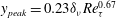 $y_{peak}=0.23{\it\delta}_{{\it\nu}}\mathit{Re}_{{\it\tau}}^{0.67}$
is the fit by Hultmark et al. (Reference Hultmark, Vallikivi, Bailey and Smits2012) of the location of the outer peak in the streamwise turbulent energy plotted in figures 2 and 4. The superposed dotted line suggests a logarithmic dependence of
$y_{peak}=0.23{\it\delta}_{{\it\nu}}\mathit{Re}_{{\it\tau}}^{0.67}$
is the fit by Hultmark et al. (Reference Hultmark, Vallikivi, Bailey and Smits2012) of the location of the outer peak in the streamwise turbulent energy plotted in figures 2 and 4. The superposed dotted line suggests a logarithmic dependence of
 $(1-y/{\it\delta}-(\text{d}\overline{u}_{+}/\text{d}y^{+}))(\text{d}\overline{u}_{+}/\text{d}\ln y^{+})$
on
$(1-y/{\it\delta}-(\text{d}\overline{u}_{+}/\text{d}y^{+}))(\text{d}\overline{u}_{+}/\text{d}\ln y^{+})$
on
 $y/{\it\delta}$
at the right of the peak.
$y/{\it\delta}$
at the right of the peak.

In figure 10 we use the NSTAP Superpipe data to plot
 $(1-y/{\it\delta}-(\text{d}\overline{u}_{+}/\text{d}y^{+}))$
as a function of
$(1-y/{\it\delta}-(\text{d}\overline{u}_{+}/\text{d}y^{+}))$
as a function of
 $y/{\it\delta}$
in one case and
$y/{\it\delta}$
in one case and
 $y^{+}$
in the other. As these are pipe data, the plots in figure 10 are effectively plots of the normalised Reynolds stress
$y^{+}$
in the other. As these are pipe data, the plots in figure 10 are effectively plots of the normalised Reynolds stress
 $-\langle u^{\prime }v^{\prime }\rangle /u_{{\it\tau}}^{2}$
. It is clear that
$-\langle u^{\prime }v^{\prime }\rangle /u_{{\it\tau}}^{2}$
. It is clear that
 $-\langle u^{\prime }v^{\prime }\rangle \approx u_{{\it\tau}}^{2}$
only if
$-\langle u^{\prime }v^{\prime }\rangle \approx u_{{\it\tau}}^{2}$
only if
 $\mathit{Re}_{{\it\tau}}>40\,000$
and for distances from the wall such that
$\mathit{Re}_{{\it\tau}}>40\,000$
and for distances from the wall such that
 $100<y^{+}$
and
$100<y^{+}$
and
 $y/{\it\delta}<0.01$
. (See also Zhao & Smits Reference Zhao and Smits2007 who showed that the viscous contribution to the total stress is less that 1 % at
$y/{\it\delta}<0.01$
. (See also Zhao & Smits Reference Zhao and Smits2007 who showed that the viscous contribution to the total stress is less that 1 % at
 $y^{+}>250$
.) It of course remains perfectly true that
$y^{+}>250$
.) It of course remains perfectly true that
 $-\langle u^{\prime }v^{\prime }\rangle /u_{{\it\tau}}^{2}$
is a linear function of
$-\langle u^{\prime }v^{\prime }\rangle /u_{{\it\tau}}^{2}$
is a linear function of
 $y/{\it\delta}$
at a distance of a few hundred wall units from the walls but it is also true that this linear dependence is small compared to 1 (the leading term) for
$y/{\it\delta}$
at a distance of a few hundred wall units from the walls but it is also true that this linear dependence is small compared to 1 (the leading term) for
 $y/{\it\delta}$
smaller than
$y/{\it\delta}$
smaller than
 $O(10^{-2})$
. The resulting intermediate range of wall distances
$O(10^{-2})$
. The resulting intermediate range of wall distances
 $y$
where
$y$
where
 $-\langle u^{\prime }v^{\prime }\rangle \approx u_{{\it\tau}}^{2}$
is a good approximation requires
$-\langle u^{\prime }v^{\prime }\rangle \approx u_{{\it\tau}}^{2}$
is a good approximation requires
 $\mathit{Re}_{{\it\tau}}$
to be larger than
$\mathit{Re}_{{\it\tau}}$
to be larger than
 $O(10^{4})$
to exist. At values of
$O(10^{4})$
to exist. At values of
 $y$
larger than
$y$
larger than
 ${\it\delta}/10$
the normalised Reynolds stress decreases abruptly towards 0 which explains why the left-hand side of (6.2) does the same in figures 7–9 at these values of
${\it\delta}/10$
the normalised Reynolds stress decreases abruptly towards 0 which explains why the left-hand side of (6.2) does the same in figures 7–9 at these values of
 $y$
.
$y$
.
Normalised Reynolds stress
 $-\langle u^{\prime }v^{\prime }\rangle /u_{{\it\tau}}^{2}$
calculated from the NSTAP Superpipe mean flow data of Hultmark et al. (Reference Hultmark, Vallikivi, Bailey and Smits2012, Reference Hultmark, Vallikivi, Bailey and Smits2013) as
$-\langle u^{\prime }v^{\prime }\rangle /u_{{\it\tau}}^{2}$
calculated from the NSTAP Superpipe mean flow data of Hultmark et al. (Reference Hultmark, Vallikivi, Bailey and Smits2012, Reference Hultmark, Vallikivi, Bailey and Smits2013) as
 $(1-y/{\it\delta}-(\text{d}\overline{u}_{+}/\text{d}y^{+}))$
(for turbulent pipe flow) versus
$(1-y/{\it\delta}-(\text{d}\overline{u}_{+}/\text{d}y^{+}))$
(for turbulent pipe flow) versus
 $y^{+}$
(a) and versus
$y^{+}$
(a) and versus
 $y/{\it\delta}$
(b). Here
$y/{\it\delta}$
(b). Here
 $\mathit{Re}_{{\it\tau}}$
ranges from about 2000 to about 100 000.
$\mathit{Re}_{{\it\tau}}$
ranges from about 2000 to about 100 000.

Figure 10 makes it clear that (6.2) simplifies to
 $$\begin{eqnarray}\frac{\text{d}\overline{u}_{+}}{\text{d}\ln y^{+}}\approx C_{s}E^{+}\end{eqnarray}$$
in turbulent pipe flow only if
 $\mathit{Re}_{{\it\tau}}>40\,000$
and only in the range
$\mathit{Re}_{{\it\tau}}>40\,000$
and only in the range
 $100{\it\delta}_{{\it\nu}}<y<{\it\delta}/100$
. Using the attached eddy model’s
$100{\it\delta}_{{\it\nu}}<y<{\it\delta}/100$
. Using the attached eddy model’s
 $E^{+}\approx M_{0}+M_{1}\ln ({\it\delta}/y)$
in the range
$E^{+}\approx M_{0}+M_{1}\ln ({\it\delta}/y)$
in the range
 $y_{\ast }<y\ll {\it\delta}$
we obtain the following asymptotic form of the mean flow profile in
$y_{\ast }<y\ll {\it\delta}$
we obtain the following asymptotic form of the mean flow profile in
 $y_{\ast }<y<0.01{\it\delta}$
(as
$y_{\ast }<y<0.01{\it\delta}$
(as
 $y_{\ast }$
is larger than
$y_{\ast }$
is larger than
 $100{\it\delta}_{{\it\nu}}$
):
$100{\it\delta}_{{\it\nu}}$
):
 $$\begin{eqnarray}\overline{u}_{+}\approx C_{s}M_{0}\ln (y/{\it\delta})-\frac{C_{s}M_{1}}{2}[\ln (y/{\it\delta})]^{2}+M_{2}\end{eqnarray}$$
in terms of an extra integration constant
 $M_{2}$
. We stress again the limited
$M_{2}$
. We stress again the limited
 $y$
-range of validity of this high-Reynolds-number mean flow profile (to the right of the outer peak) and that it can only be expected at
$y$
-range of validity of this high-Reynolds-number mean flow profile (to the right of the outer peak) and that it can only be expected at
 $\mathit{Re}_{{\it\tau}}>40\,000$
. This
$\mathit{Re}_{{\it\tau}}>40\,000$
. This
 $y$
-range can be made longer if we do not use
$y$
-range can be made longer if we do not use
 $-\langle u^{\prime }v^{\prime }\rangle \approx u_{{\it\tau}}^{2}$
which leads to (6.3) but
$-\langle u^{\prime }v^{\prime }\rangle \approx u_{{\it\tau}}^{2}$
which leads to (6.3) but
 $-\langle u^{\prime }v^{\prime }\rangle \approx u_{{\it\tau}}^{2}\approx 1-y/{\it\delta}$
which holds for
$-\langle u^{\prime }v^{\prime }\rangle \approx u_{{\it\tau}}^{2}\approx 1-y/{\it\delta}$
which holds for
 $y/{\it\delta}_{{\it\nu}}$
larger than
$y/{\it\delta}_{{\it\nu}}$
larger than
 $O(100)$
and leads to
$O(100)$
and leads to
 $(1-y/{\it\delta})(\text{d}\overline{u}_{+}/\text{d}\ln y^{+})\approx C_{s}E^{+}$
in place of (6.3).
$(1-y/{\it\delta})(\text{d}\overline{u}_{+}/\text{d}\ln y^{+})\approx C_{s}E^{+}$
in place of (6.3).
As shown in § 5,
 $E^{+}\approx M_{0}+M_{1}\ln ({\it\delta}/y)$
and therefore also (6.4) are based on the additional assumption that any intermittency which might exist in the fluctuating wall shear stress is of such a nature that the Townsend–Perry spectral scalings
$E^{+}\approx M_{0}+M_{1}\ln ({\it\delta}/y)$
and therefore also (6.4) are based on the additional assumption that any intermittency which might exist in the fluctuating wall shear stress is of such a nature that the Townsend–Perry spectral scalings
 $E_{11}(k_{1},y)\sim u_{{\it\tau}}^{2}k_{1}^{-1}$
remain intact. Otherwise one can expect power laws of
$E_{11}(k_{1},y)\sim u_{{\it\tau}}^{2}k_{1}^{-1}$
remain intact. Otherwise one can expect power laws of
 $y/{\it\delta}$
instead of logarithms of
$y/{\it\delta}$
instead of logarithms of
 $y/{\it\delta}$
in the formula for the mean flow profile (6.4).
$y/{\it\delta}$
in the formula for the mean flow profile (6.4).
We close this section with a comment on the mesolayer, a concept introduced by Long & Chen (Reference Long and Chen1981) and most recently discussed by Vallikivi, Ganapathisubramani & Smits (Reference Vallikivi, Ganapathisubramani and Smits2014) who also provide a list of relevant references. In the present paper, profiles have been obtained for
 $\overline{u^{\prime 2}}(y)$
in the range
$\overline{u^{\prime 2}}(y)$
in the range
 ${\it\delta}_{{\it\nu}}\ll y\ll {\it\delta}$
and for
${\it\delta}_{{\it\nu}}\ll y\ll {\it\delta}$
and for
 $\overline{u}(y)$
in the range
$\overline{u}(y)$
in the range
 $y_{P{\it\epsilon}}<y<0.01{\it\delta}$
where production has been assumed to balance dissipation. George & Castillo (Reference George and Castillo1997) argued that the mesolayer is a region from
$y_{P{\it\epsilon}}<y<0.01{\it\delta}$
where production has been assumed to balance dissipation. George & Castillo (Reference George and Castillo1997) argued that the mesolayer is a region from
 $y^{+}\simeq 30$
to
$y^{+}\simeq 30$
to
 $y^{+}\simeq 300$
where, owing to low turbulent Reynolds number
$y^{+}\simeq 300$
where, owing to low turbulent Reynolds number
 $y^{+}$
values, the dissipation does not have its high-Reynolds-number scaling and the Kolmogorov range (iv) of our spectral model in § 4 is effectively absent. This has no bearing on our calculations of §§ 4 and 5 because the energy in the Kolmogorov range (iv) is small compared with the other ranges and the outer peak comes from the new small wavenumber range (ii). (In fact it is easy to check that the Kolmogorov range in the Townsend–Perry model cannot, by itself, lead to an outer turbulent energy peak.) However, it might be that we cannot use the scaling
$y^{+}$
values, the dissipation does not have its high-Reynolds-number scaling and the Kolmogorov range (iv) of our spectral model in § 4 is effectively absent. This has no bearing on our calculations of §§ 4 and 5 because the energy in the Kolmogorov range (iv) is small compared with the other ranges and the outer peak comes from the new small wavenumber range (ii). (In fact it is easy to check that the Kolmogorov range in the Townsend–Perry model cannot, by itself, lead to an outer turbulent energy peak.) However, it might be that we cannot use the scaling
 ${\it\tau}\sim y/u_{{\it\tau}}$
at
${\it\tau}\sim y/u_{{\it\tau}}$
at
 $y^{+}\lesssim 300$
and that our approach for obtaining the mean flow gradient profile might therefore be valid only in the region
$y^{+}\lesssim 300$
and that our approach for obtaining the mean flow gradient profile might therefore be valid only in the region
 $\max (300{\it\delta}_{{\it\nu}},y_{P{\it\epsilon}})<y\ll 0.01{\it\delta}$
. Note that the value of
$\max (300{\it\delta}_{{\it\nu}},y_{P{\it\epsilon}})<y\ll 0.01{\it\delta}$
. Note that the value of
 $y_{peak}$
in the Princeton NSTAP data is about
$y_{peak}$
in the Princeton NSTAP data is about
 $300{\it\delta}_{{\it\nu}}$
at
$300{\it\delta}_{{\it\nu}}$
at
 $\mathit{Re}_{{\it\tau}}\approx 40\,000$
and about
$\mathit{Re}_{{\it\tau}}\approx 40\,000$
and about
 $500{\it\delta}_{{\it\nu}}$
at
$500{\it\delta}_{{\it\nu}}$
at
 $\mathit{Re}_{{\it\tau}}\approx 100\,000$
, which means that the mesolayer is indeed under
$\mathit{Re}_{{\it\tau}}\approx 100\,000$
, which means that the mesolayer is indeed under
 $y_{peak}$
for
$y_{peak}$
for
 $\mathit{Re}_{{\it\tau}}>40\,000$
. The prediction that the mean flow gradient has an outer peak at the same distance from the wall where the streamwise turbulence intensity has an outer peak has been based on the assumption that
$\mathit{Re}_{{\it\tau}}>40\,000$
. The prediction that the mean flow gradient has an outer peak at the same distance from the wall where the streamwise turbulence intensity has an outer peak has been based on the assumption that
 $y_{P{\it\epsilon}}<y_{peak}$
. The region where production and dissipation balance and where turbulent transport has negligible effects may or may not be expected to have an overlap with the mesolayer. The task of working out the scalings of
$y_{P{\it\epsilon}}<y_{peak}$
. The region where production and dissipation balance and where turbulent transport has negligible effects may or may not be expected to have an overlap with the mesolayer. The task of working out the scalings of
 $y_{P{\it\epsilon}}$
and how it compares with
$y_{P{\it\epsilon}}$
and how it compares with
 $300{\it\delta}_{{\it\nu}}$
must be left for a future study which will have the means to address these questions.
$300{\it\delta}_{{\it\nu}}$
must be left for a future study which will have the means to address these questions.
7. Conclusion
In way of conclusion we list the main points made in this paper.
-
(i) For the Townsend–Perry
$k_{1}^{-1}$
spectrum to be viable, i.e. to be compatible with a realistic integral scale dependence on
$y$
, we need to add to the Perry et al. (Reference Perry, Henbest and Chong1986) spectral model an extra wavenumber range at wavenumbers smaller than those where
$E_{11}(k_{1},y)\sim u_{{\it\tau}}^{2}k_{1}^{-1}$
. -
(ii) Simple modelling of this range (see § 4) implies the existence of an outer peak in the streamwise turbulence kinetic energy at a
$y$
-position
$y_{peak}$
which grows with respect to
${\it\delta}_{{\it\nu}}$
and decreases with respect to
${\it\delta}$
as
$\mathit{Re}_{{\it\tau}}$
increases. The streamwise kinetic energy at that peak grows logarithmically with
$\mathit{Re}_{{\it\tau}}$
. -
(iii) The functional form which results from our modified Townsend–Perry model and which may be useful as a starting point in future investigations is the following: in the range
${\it\delta}_{{\it\nu}}\ll y<y_{\ast }\sim {\it\delta}\mathit{Re}_{{\it\tau}}^{-1/3}$
(7.1)where all of the constants are independent of
$$\begin{eqnarray}{\textstyle \frac{1}{2}}\overline{u^{\prime 2}}(y)/u_{{\it\tau}}^{2}\approx C_{s0}-C_{s1}\ln ({\it\delta}/y)-C_{s2}(y/{\it\delta})^{d}\mathit{Re}_{{\it\tau}}^{d/3}\end{eqnarray}$$
$y$
,
${\it\delta}$
,
${\it\nu}$
and
$\mathit{Re}_{{\it\tau}}$
except for
$C_{s0}$
which may be a logarithmically increasing function of
$\mathit{Re}_{{\it\tau}}$
; in the range
$y_{\ast }<y\ll {\it\delta}$
(7.2)as predicted by Townsend (Reference Townsend1976) and Perry et al. (Reference Perry, Henbest and Chong1986).
$$\begin{eqnarray}{\textstyle \frac{1}{2}}\overline{u^{\prime 2}}(y)/u_{{\it\tau}}^{2}\approx C_{3}+C_{4}\ln ({\it\delta}/y)\end{eqnarray}$$
-
(iv) The very high-
$\mathit{Re}_{{\it\tau}}$
Princeton Superpipe NSTAP data used here and the turbulent channel flow DNS of Dallas et al. (Reference Dallas, Vassilicos and Hewitt2009) support the view that it is the eddy turnover time
${\it\tau}\equiv E/{\it\epsilon}$
that is independent of
${\it\nu}$
and
${\it\delta}$
in the range
${\it\delta}_{{\it\nu}}\ll y\ll {\it\delta}$
rather than the mean flow gradient. This implies
${\it\tau}\sim y/u_{{\it\tau}}$
in that range, a relation which can serve as a unifying principle across Reynolds numbers in turbulent pipe/channel flows. Of course, further research is needed to fully establish such a unifying principle. -
(v) The mean flow profile and scalings can be obtained from
${\it\tau}\sim y/u_{{\it\tau}}$
if enough is known about the production–dissipation balance/imbalance. Here we have assumed that production and dissipation balance in a range
$y_{P{\it\epsilon}}<y\ll {\it\delta}$
where
$y_{P{\it\epsilon}}$
is smaller than
$y_{peak}$
. Due to this balance, a profile for
$E^{+}$
similar to that of
$\overline{u^{\prime 2}}/u_{{\it\tau}}^{2}$
implies that
$(1-y/{\it\delta}-(\text{d}\overline{u}_{+}/\text{d}y^{+}))(\text{d}\overline{u}_{+}/\text{d}\ln y^{+})$
(i) has an outer peak at the same position
$y=y_{peak}$
where
$\overline{u^{\prime 2}}/u_{{\it\tau}}^{2}$
has an outer peak, and (ii) decreases with distance from the wall as a function of
$\ln ({\it\delta}/y)$
where
$y_{\ast }<y\ll {\it\delta}$
. In the intermediate range of wall distances where
$-\langle u^{\prime }v^{\prime }\rangle \approx u_{{\it\tau}}^{2}$
is a good approximation (see point 6 below), these two conclusions hold for
$\text{d}\overline{u}_{+}/\text{d}\ln y^{+}$
. The very high
$\mathit{Re}_{{\it\tau}}$
NSTAP Princeton Superpipe data show clear evidence in support of these conclusions. -
(vi) The same data also show that the Reynolds stress
$\langle u^{\prime }v^{\prime }\rangle$
is approximately equal to
$-u_{{\it\tau}}^{2}$
only if
$\mathit{Re}_{{\it\tau}}>40\,000$
and for distances from the wall such that
$100<y^{+}$
,
$y/{\it\delta}<0.01$
. The balance
$-\langle u^{\prime }v^{\prime }\rangle (\text{d}\overline{u}/\text{d}y)\approx {\it\epsilon}$
and the kinetic energy profile
$E^{+}\approx M_{0}+M_{1}\ln ({\it\delta}/y)$
(where
$M_{0}$
and
$M_{1}$
are dimensionless constants) in
$y_{\ast }\ll y\ll {\it\delta}$
therefore imply in terms of an integration constant
$M_{2}$
that (7.3)in
$$\begin{eqnarray}\overline{u}_{+}\approx C_{s}M_{0}\ln (y/{\it\delta})-\frac{C_{s}M_{1}}{2}[\ln (y/{\it\delta})]^{2}+M_{2}\end{eqnarray}$$
$y_{\ast }<y<0.01{\it\delta}$
provided that
$\mathit{Re}_{{\it\tau}}>40\,000$
. This is the modified log-law of the wall.


Acknowledgements
We are very grateful to Dr M. Vallikivi and Professor A. J. Smits for kindly providing us with their NSTAP Superpipe data (first published in Hultmark et al. Reference Hultmark, Vallikivi, Bailey and Smits2012, Reference Hultmark, Vallikivi, Bailey and Smits2013) and with energy spectra from the same measurements. This work was supported by Campus International pour la Sécurité et l’Intermodalité des Transports, la Région Nord-Pas-de-Calais, l’Union Européenne, la Direction de la Recherche, Enseignement Supérieur, Santé et Technologies de l’Information et de la Communication et le Centre National de la Recherche Scientifique. J.C.V. acknowledges the support of an ERC advanced grant (2013–2018).


 Open access