


1. Introduction
In turbulence modelling, the Navier–Stokes equations serve as the foundation for deriving evolution equations of coarse-grained statistical quantities, which in turn provide closure for the coarse-grained equations themselves. The coarse-graining procedure, introduced to mitigate computational expense, depends on the choice of averaging or filtering operator – such as ensemble, temporal or spatial averaging – selected according to the modelling framework. Application of this operator yields statistical moments that may be formulated as single- or multi-point, higher-order quantities. Owing to the prevalence of spatial derivatives in the governing equations, multi-point statistics offer a natural description of turbulent interactions. Nevertheless, most practical turbulence models employ single-point closures to reduce cost and analytical complexity, necessitating additional modelling assumptions to represent intrinsically multi-point phenomena.
Single-point closures often fail to accurately account for non-local interactions, anisotropy and energy transfer across scales with sufficient fidelity. Two-point closures, such as the eddy damped quasi-normal Markovian (EDQNM) (Orszag Reference Orszag1970), test-field models (Kraichnan Reference Kraichnan1971), direct interaction approximation (DIA) (Kraichnan Reference Kraichnan1959) and related approaches, address many of these limitations, albeit demonstrated in canonical, and often homogeneous turbulence. These offer explicit representations of the two-point correlation functions which directly model scale-to-scale energy transfer. Two-point methods also allow representation of structural and wave effects – e.g. rotation and stratification – that are essentially inaccessible to simpler closures (Sagaut & Cambon Reference Sagaut and Cambon2018). Another advantage of two-point closures is the reduced reliance on empirical constants; in some formulations, closures can predict or constrain what would otherwise be ad hoc parameters in single-point or lower-order models (Bos & Bertoglio Reference Bos and Bertoglio2006). Two-point closures also naturally reduce to rapid distortion theory (RDT) in the rapid distortion/linear limit. This limiting behaviour can be exploited in problems where the turbulence does not have time to interact with itself and the turbulence dynamics is significantly simplified, circumventing the closure problem in some special cases. Collectively, these advantages make two-point closures an appealing framework for flows where non-locality, anisotropy and details of energy transfer are important.
Historically, most two-point turbulence closures have been formulated in spectral space, where the governing equations for two-point velocity correlations simplify considerably due to statistical homogeneity. Classical models such as EDQNM and DIA operate on the energy spectrum and directly capture triadic interactions across wavenumbers (Orszag Reference Orszag1970; Lesieur & Schertzer Reference Lesieur and Schertzer1978). Spectral representations make the scale-to-scale transfer terms transparent and computationally efficient to evaluate. However, spectral methods tend to be limited to special canonical cases because of the mathematical limitations of the Fourier transform, and the vast majority of spectral models are formulated for incompressible flows. Very few works in the literature focus on variable-density cases, most notably the variable-density models by Clark & Spitz (Reference Clark and Spitz1995) and Besnard et al. (Reference Besnard, Harlow, Rauenzahn and Zemach1996), and fewer on compressible flows, with the main example being the modelling work for compressible homogeneous isotropic turbulence (HIT) by Bertoglio, Bataille & Marion (Reference Bertoglio, Bataille and Marion2001). In a strict sense, application of Fourier transforms to problems with discontinuities, such as compressible flows with shocks, is ill-posed. Canuto et al. (Reference Canuto, Quarteroni, Hussaini, Zang and Thomas2007) discusses the application of spectral methods to such problems, but almost all applications are spectral collocation methods which only transform the spatial derivatives to spectral space and not the dynamical variables. Without transformation of the variables, many of the spectral-based closure ideas originally developed for higher-order turbulence moments cannot be applied to this method. Therefore, this provides motivation for development of a two-point framework that enables translation of closure ideas to more complex discontinuous problems. A natural approach to this problem is to work exclusively in physical space.
Two-point closures are less common in physical space; yet they offer several advantages: they can be extended to inhomogeneous flows, more naturally preserve the locality of boundary conditions and often provide more direct connections to experimentally measurable two-point statistics. However, some advantages of spectral methods such as exact operator representation, explicit energy transfer, structural wave effects, etc. can only be approximated in physical space because the corresponding linear operator is intrinsically non-local and necessarily relies on approximations. Notable early developments include the work of Besnard et al. (Reference Besnard, Harlow, Rauenzahn and Zemach1996), who formulated a two-point closure in physical space for variable-density turbulence but ultimately utilised a Fourier transformation, and Cambon & Rubinstein (Reference Cambon and Rubinstein2006), who advocated for real-space correlation closures as a complement to spectral models. More recently, scale-space transport equations based on the generalised Kármán–Howarth–Monin–Hill (KHMH) equations (Von Kármán & Howarth Reference Von Kármán and Howarth1938; Monin Reference Monin1959; Hill Reference Hill2002) have been derived explicitly in physical space, allowing one to track energy transfer simultaneously across spatial locations and separations. These equations have been used in many studies to analyse two-point correlations of inhomogeneous anisotropic flows, such as the work by Beaumard et al. (Reference Beaumard, Bragança, Cuvier and Vassilicos2024). Another class of these methods use the scale-space energy density function of Hamba (Reference Hamba2015). The work of Arun et al. (Reference Arun, Sameen, Srinivasan and Girimaji2021) provides an example of how the scale-space transform can be used to compute two-point correlations in inhomogeneous compressible flows. However, these studies generally do not use the KHMH equations or scale-space energy density function framework to derive closures of the moment equations; they are used as analysis/diagnostic tools for high-fidelity data. To the authors’ knowledge, there has not been development of a two-point physical-space framework that can be systematically used to convert the relevant unclosed moment partial differential equations (PDEs) into ordinary differential equations (ODEs) and apply the closure ideas originally developed for spectral methods. The purpose of this work is to begin the development of a framework that can be used for prediction.
This work will consider the closure of incompressible HIT as a starting point to demonstrate the viability of the physical-space two-point formulation and how it may be used in a predictive setting. Much work has explored HIT, including progress on two-point closures in physical space using the Kármán–Howarth equations (Von Kármán & Howarth Reference Von Kármán and Howarth1938). The early work of Domaradzki & Mellor (Reference Domaradzki and Mellor1984) and Oberlack & Peters (Reference Oberlack and Peters1993) explored closure of the Kármán–Howarth equations with an eddy-viscosity model. Further work on modelling higher-order structure functions by Thiesset et al. (Reference Thiesset, Antonia, Danaila and Djenidi2013) and Djenidi & Antonia (Reference Djenidi and Antonia2022), to name a few, has also relied on eddy-viscosity-type closures. All these methods rely on the Kármán–Howarth equations, and the underlying closures cannot be naturally extended to general problems. To the authors’ knowledge, there have not been attempts to adapt the ideas of EDQNM or DIA with the Kármán–Howarth equations. Thus, while closure of incompressible HIT is a common endeavour, the translation of the spectral closure ideas to a physical-space two-point formulation is novel.
Instead of relying on a spectral transformation, a discrete approach is taken using finite differences to approximate spatial derivatives. For example, using a simple second-order central difference to discretise a spatial derivative in a third-order moment of some dynamical variable $u_i(\boldsymbol{x})$
evaluated at spatial points
$u_i(\boldsymbol{x})$
evaluated at spatial points $\boldsymbol{x}$
and
$\boldsymbol{x}$
and $\boldsymbol{y}$
,
$\boldsymbol{y}$
,
 \begin{gather} \left\langle u_i(\boldsymbol{x}) \frac {\partial u_{\!j}(\boldsymbol{x})}{\partial x_l}u_k(\boldsymbol{y}) \right\rangle \approx \left\langle u_i(\boldsymbol{x}) \frac { u_{\!j}(\boldsymbol{x}+\Delta x_l)}{2\Delta x_l}u_k(\boldsymbol{y}) \right\rangle - \left\langle u_i(\boldsymbol{x})\frac {u_{\!j}(\boldsymbol{x}-\Delta x_l)}{2\Delta x_l}u_k(\boldsymbol{y}) \right\rangle \!, \end{gather}
enables the spatial derivatives of higher-order moments to become a summation of neighbouring moments evaluated at different correlation distances $r=\pm \Delta x_l$
. This highlights the most significant advantage of using two-point statistics over single-point statistics, as two-point information will inherently contain length-scale information, albeit truncated. This means that correlations with derivative terms do not require their own closure. Quantities such as
$r=\pm \Delta x_l$
. This highlights the most significant advantage of using two-point statistics over single-point statistics, as two-point information will inherently contain length-scale information, albeit truncated. This means that correlations with derivative terms do not require their own closure. Quantities such as
 \begin{equation} \left\langle \frac {\partial u_i}{\partial x_{\!j}}u_k \right\rangle \!,\; \left\langle u_i\frac {\partial u_{\!j}}{\partial x_l}u_k \right\rangle \end{equation}
will be closed if the higher-order two-point moments are known. Although this is not a significant advantage for simple problems such as incompressible HIT, it is important for more complex moment equations that arise in inhomogeneous anisotropic compressible turbulence, where many unclosed terms have spatial derivatives embedded into the higher-order moments.
2. Definitions and moment equations
Definitions and moment equations are now discussed with generality in mind. Simplifications are invoked later to make the problem more tractable but case-limited. A Reynolds-average coarse-graining operation is used, where average properties of the velocity field are interpreted as ensemble averages over a large number of flow realisations, denoted by $\langle \;\rangle$
. The velocity realisations are governed by the incompressible Navier–Stokes equations:
$\langle \;\rangle$
. The velocity realisations are governed by the incompressible Navier–Stokes equations:
 \begin{equation} \frac {\partial u_i(\boldsymbol{x})}{\partial t}=-u_{\!j}(\boldsymbol{x})\frac {\partial u_i(\boldsymbol{x})}{\partial x_{\!j}}-\frac {1}{\rho }\frac {\partial p(\boldsymbol{x})}{\partial x_i}+\nu \frac {\partial ^2u_i(\boldsymbol{x})}{\partial x_{\!j}^2}, \end{equation}
 \begin{equation} \frac {\partial u_i}{\partial x_i}=0, \end{equation}
where $u_i(\boldsymbol{x})$
is the instantaneous
$u_i(\boldsymbol{x})$
is the instantaneous $i{\text{th}}$
velocity component evaluated at
$i{\text{th}}$
velocity component evaluated at $\boldsymbol{x}$
in three-dimensional space,
$\boldsymbol{x}$
in three-dimensional space, $p$
is the pressure,
$p$
is the pressure, $\rho$
is the density and
$\rho$
is the density and $\nu$
is the kinematic viscosity. The pressure is closed by differentiating the momentum equation and solving the pressure–Poisson equation with the free-space Green function
$\nu$
is the kinematic viscosity. The pressure is closed by differentiating the momentum equation and solving the pressure–Poisson equation with the free-space Green function $1/4\pi |\boldsymbol{x}{-}\boldsymbol{x}'|$
(Durbin & Pettersson-Reif Reference Durbin and Pettersson-Reif2011):
$1/4\pi |\boldsymbol{x}{-}\boldsymbol{x}'|$
(Durbin & Pettersson-Reif Reference Durbin and Pettersson-Reif2011):
 \begin{equation} \frac {1}{\rho }\frac {\partial p(\boldsymbol{x})}{\partial x_i}=-\frac {1}{4\pi }\iiint _{-\infty }^{\infty }\frac {\partial }{\partial x'_i}\left (\frac {\partial u_{\!j}(\boldsymbol{x}')}{\partial x'_k}\frac {\partial u_k(\boldsymbol{x}')}{\partial x'_{\!j}}\frac {1}{|\boldsymbol{x}-\boldsymbol{x}'|}\right ){\rm d}^3\boldsymbol{x}'. \end{equation}
The general statistical quantities of interest are the multi-point moments
 \begin{equation} R_{\textit{ij}..k}(\boldsymbol{x},\boldsymbol{y},..,\boldsymbol{z})\triangleq \langle u_i(\boldsymbol{x})u_{\!j}(\boldsymbol{y})..u_k(\boldsymbol{z})\rangle \end{equation}
or more specifically the two-point velocity moment tensor, defined as
 \begin{equation} R_{\textit{ij}}(\boldsymbol{x},\boldsymbol{y})\triangleq \langle u_i(\boldsymbol{x})u_{\!j}(\boldsymbol{y})\rangle . \end{equation}
The second-order moment can also be written as a function of the distance vector between the two points by substituting $\boldsymbol{y}=\boldsymbol{x}+\boldsymbol{r}$
. This work will only consider two-point statistical quantities but uses higher-order two-point moments in the closure scheme.
$\boldsymbol{y}=\boldsymbol{x}+\boldsymbol{r}$
. This work will only consider two-point statistical quantities but uses higher-order two-point moments in the closure scheme.
Now, the evolution equations for the two-point second- and third-order moments can be derived. To simplify notation, we introduce the multi-point spatial derivative of higher-order moments:
 \begin{equation} \frac {\partial R_{\textit{ijk}}(\boldsymbol{x},\boldsymbol{y},\boldsymbol{z})}{\partial y_l}\Bigg |_{y=x}\triangleq \left\langle u_i(\boldsymbol{x}) \frac {\partial u_{\!j}(\boldsymbol{x})}{\partial x_l}u_k(\boldsymbol{z}) \right\rangle \!, \end{equation}
where the conditional removes ambiguity by distinguishing which term in the moment the differential operator acts upon if two or more terms are evaluated at the same spatial point. The product rule is applied to $R_{\textit{ij}}(\boldsymbol{x},\boldsymbol{y})$
, and since the time derivative is a linear operator, we can use (2.1) to derive the second- and third-moment evolution equations:
$R_{\textit{ij}}(\boldsymbol{x},\boldsymbol{y})$
, and since the time derivative is a linear operator, we can use (2.1) to derive the second- and third-moment evolution equations:
 \begin{align} &\frac {\partial R_{\textit{ij}}(\boldsymbol{x},\boldsymbol{y})}{\partial t}=-\frac {\partial R_{\textit{kij}}(\boldsymbol{x},\boldsymbol{z},\boldsymbol{y})}{\partial z_k}\Bigg |_{z=x}-\frac {\partial R_{\textit{ijk}}(\boldsymbol{x},\boldsymbol{z},\boldsymbol{y})}{\partial z_k}\Bigg |_{z=y} \nonumber\\ &\qquad-\frac {1}{\rho } \left(\left\langle \frac {\partial p(\boldsymbol{x})}{\partial x_i}u_{\!j}(\boldsymbol{y}) \right\rangle + \left\langle \frac {\partial p(\boldsymbol{y})}{\partial y_{\!j}}u_i(\boldsymbol{x}) \right\rangle \right) +\nu \frac {\partial ^2 R_{\textit{ij}}(\boldsymbol{x},\boldsymbol{y})}{\partial x_k^2}+\nu \frac {\partial ^2 R_{\textit{ij}}(\boldsymbol{x},\boldsymbol{y})}{\partial y_k^2}, \end{align}
 \begin{align} &\frac {\partial R_{\textit{ijk}}(\boldsymbol{x},\boldsymbol{y},\boldsymbol{z})}{\partial t}=-\frac {\partial R_{\textit{lijk}}(\boldsymbol{x},\boldsymbol{w},\boldsymbol{y},\boldsymbol{z})}{\partial w_l}\Bigg |_{w=x}-\frac {\partial R_{\textit{ljik}}(\boldsymbol{y},\boldsymbol{w},\boldsymbol{x},\boldsymbol{z})}{\partial w_l}\Bigg |_{w=y}-\frac {\partial R_{\textit{lkij}}(\boldsymbol{z},\boldsymbol{w},\boldsymbol{x},\boldsymbol{y})}{\partial w_l}\Bigg |_{w=z} \nonumber\\ &\qquad -\frac {1}{\rho } \left( \left\langle \frac {\partial p(\boldsymbol{x})}{\partial x_i}u_{\!j}(\boldsymbol{y})u_k(\boldsymbol{z}) \right\rangle + \left\langle \frac {\partial p(\boldsymbol{y})}{\partial y_{\!j}}u_i(\boldsymbol{x})u_k(\boldsymbol{z}) \right\rangle + \left\langle \frac {\partial p(\boldsymbol{z})}{\partial z_k}u_i(\boldsymbol{x})u_{\!j}(\boldsymbol{y}) \right\rangle \right) \nonumber\\ &\qquad +\nu \frac {\partial ^2 R_{\textit{ijk}}(\boldsymbol{x},\boldsymbol{y},\boldsymbol{z})}{\partial x_k^2}+\nu \frac {\partial ^2 R_{\textit{ijk}}(\boldsymbol{x},\boldsymbol{y},\boldsymbol{z})}{\partial y_k^2}+\nu \frac {\partial ^2 R_{\textit{ijk}}(\boldsymbol{x},\boldsymbol{y},\boldsymbol{z})}{\partial z_k^2}. \end{align}
From (2.7)–(2.8), it is apparent that each moment equation requires information from the next higher-order moment. This is the closure problem, and is discussed in § 3. To simplify the problem, we assume that the turbulence is statistically homogeneous and isotropic. Extension to general problems is discussed later in this paper. The HIT properties allow for the two-point velocity moment to be written in terms of the one-dimensional longitudinal function $f(r)$
and the correlation distance vector
$f(r)$
and the correlation distance vector $\boldsymbol{r}$
(Durbin & Pettersson-Reif Reference Durbin and Pettersson-Reif2011):
$\boldsymbol{r}$
(Durbin & Pettersson-Reif Reference Durbin and Pettersson-Reif2011):
 \begin{equation} R_{\textit{ij}}(\boldsymbol{r})= u^{\prime 2}\left (f(r)\delta _{\textit{ij}}+\frac {r}{2}\frac {{d} f(r)}{\partial r}\left (\delta _{\textit{ij}}-\frac {r_ir_{\!j}}{r^2}\right )\right ), \end{equation}
where $u'=\sqrt {u_iu_i/3}$
is the root-mean-square velocity fluctuation per component. In HIT, the trace of the two-point velocity moment is the primary statistical quantity of interest. Hence, the dimensionality of the problem is reduced because
$u'=\sqrt {u_iu_i/3}$
is the root-mean-square velocity fluctuation per component. In HIT, the trace of the two-point velocity moment is the primary statistical quantity of interest. Hence, the dimensionality of the problem is reduced because $R_{ii}(r)$
is uniquely described by the one-dimensional longitudinal function and the correlation distance magnitude
$R_{ii}(r)$
is uniquely described by the one-dimensional longitudinal function and the correlation distance magnitude $r$
. Imposing the constraints of incompressible HIT, the longitudinal function is related to the lateral function through
$r$
. Imposing the constraints of incompressible HIT, the longitudinal function is related to the lateral function through
 \begin{equation} g(r)= f(r)+\frac {r}{2}\frac {{d}f(r)}{{\rm d}r}. \end{equation}
Finally, zero mean flow $\langle u_i\rangle =0$
and statistical homogeneity imply symmetry under permutation of points and indices and translational invariance:
$\langle u_i\rangle =0$
and statistical homogeneity imply symmetry under permutation of points and indices and translational invariance:
 \begin{equation} R_{\textit{ij}..k}(\boldsymbol{x}+a,\boldsymbol{y}+a,..,\boldsymbol{z}+a)=R_{\textit{ij}..k}(\boldsymbol{x},\boldsymbol{y},..,\boldsymbol{z}). \end{equation}
2.1. Spectral moments and transformation between spaces
Now, the spectral definitions are established strictly for homogeneous turbulence with zero mean flow $\langle u_i\rangle =0$
. The multi-point
$\langle u_i\rangle =0$
. The multi-point $n{\text{th}}$
-order moments are related to the moments in Fourier space through the Fourier transform:
$n{\text{th}}$
-order moments are related to the moments in Fourier space through the Fourier transform:
 \begin{align} \hat {R}_{\textit{ij}..k}(\boldsymbol{\kappa },\boldsymbol{p}..\boldsymbol{q})&\triangleq \langle \hat {u}_i(\boldsymbol{k})\hat {u}_{\!j}(\boldsymbol{p})\ldots \hat {u}_k(\boldsymbol{q})\rangle \nonumber \\ & =\frac {1}{(2\pi )^{3(n-1)}}\int \langle u_i(\boldsymbol{x})u_{\!j}(\boldsymbol{y})\ldots u_k(\boldsymbol{z})\rangle {\rm e}^{-\mathrm{i}\boldsymbol{\kappa }\boldsymbol{\cdot }\boldsymbol{x}-\mathrm{i}\boldsymbol{p}\boldsymbol{\cdot }\boldsymbol{y}-\ldots -\mathrm{i}\boldsymbol{q}\boldsymbol{\cdot }\boldsymbol{z}}\,{\rm d}^3\boldsymbol{x}{\rm d}^3\boldsymbol{y}\ldots {\rm d}^3\boldsymbol{z}. \nonumber \\ \end{align}
Note that the trial function is the negative exponential instead of the positive one as seen in most Fourier transform definitions. We follow this notation to be consistent with Orszag (Reference Orszag1970). In spectral space, the property $\boldsymbol{\kappa }+\boldsymbol{p}+\cdots +\boldsymbol{q}=0$
arises from homogeneity due to translational invariance. This relation removes the functional dependence on the
$\boldsymbol{\kappa }+\boldsymbol{p}+\cdots +\boldsymbol{q}=0$
arises from homogeneity due to translational invariance. This relation removes the functional dependence on the $n{\textrm {th}}$
wavevector. This simplification is used throughout the remainder of the paper when working in spectral space. Another subtle restriction is that, in integrals over triadic interactions, we must avoid double-counting symmetric configurations. This implies that wavevector interactions must be non-degenerate, i.e. third-order spectral moments must obey the condition
$n{\textrm {th}}$
wavevector. This simplification is used throughout the remainder of the paper when working in spectral space. Another subtle restriction is that, in integrals over triadic interactions, we must avoid double-counting symmetric configurations. This implies that wavevector interactions must be non-degenerate, i.e. third-order spectral moments must obey the condition $\boldsymbol{\kappa }\neq {-}\boldsymbol{p}\neq \boldsymbol{q}\neq -\boldsymbol{\kappa }$
(Orszag Reference Orszag1970).
$\boldsymbol{\kappa }\neq {-}\boldsymbol{p}\neq \boldsymbol{q}\neq -\boldsymbol{\kappa }$
(Orszag Reference Orszag1970).
The HIT properties enable the representation of the spectral velocity second moments using the wavenumber-dependent spherically symmetric energy spectrum $E(\kappa )$
and wavevector
$E(\kappa )$
and wavevector $\boldsymbol{\kappa }$
:
$\boldsymbol{\kappa }$
:
 \begin{equation} \langle \hat {u}_i(\boldsymbol{k})\hat {u}_{\!j}(\boldsymbol{p})\rangle =\frac {E(\kappa )}{4\pi \kappa ^2}\left (\delta _{\textit{ij}}-\frac {\kappa _i\kappa _{\!j}}{\kappa ^2}\right )\delta (\boldsymbol{\kappa} + \boldsymbol{p}). \end{equation}
This is used to formally define the turbulent kinetic energy and turbulent dissipation rate:
 \begin{gather} \frac {1}{2}q^2\triangleq \int _0^{\infty }E(\kappa ){\rm d}\kappa =\frac {3}{2}u^{\prime 2}, \end{gather}
 \begin{gather} \epsilon \triangleq 2\nu \int _0^{\infty }\kappa ^2E(\kappa ){\rm d}\kappa =-15\nu u^{\prime 2} \frac {{\rm d}^2\kern-1pt f(r)}{{\rm d}r^2}\Bigg |_{r=0}. \end{gather}
Now, following a similar procedure to that in physical space, the moment equations are derived in spectral space:
 \begin{align} &\left [\frac {{\rm d}}{{\rm d}t}+2\nu \kappa ^2\right ]\hat {R}_{\textit{ij}}(\boldsymbol{\kappa },t) = -\frac {\mathrm{i}}{2}\int \left [P_{ikl}(\boldsymbol{\kappa })\hat {R}_{\textit{jkl}}(-\boldsymbol{\kappa },\boldsymbol{p},t)+P_{\textit{jkl}}(-\boldsymbol{\kappa })\hat {R}_{ikl}(\boldsymbol{\kappa },\boldsymbol{p},t)\right ]{\rm d}^3\boldsymbol{p}, \\[-12pt]\nonumber \end{align}
 \begin{align} &\left [\frac {{\rm d}}{{\rm d}t}+2\nu (\kappa ^2+p^2+q^2)\right ]\hat {R}_{\textit{ijk}}(\boldsymbol{\kappa },\boldsymbol{p},t)=-\frac {\mathrm{i}}{2}\int \big[P_{\textit{ilm}}(\boldsymbol{\kappa })\hat {R}_{\textit{jklm}}(\boldsymbol{p},\boldsymbol{q},\boldsymbol{r},t) \big. \nonumber\\ & \big.\qquad \qquad \qquad +P_{\textit{jlm}}(\boldsymbol{p})\hat {R}_{\textit{iklm}}(\boldsymbol{\kappa },\boldsymbol{q},\boldsymbol{r},t)+P_{\textit{klm}}(\boldsymbol{q})\hat {R}_{\textit{ijlm}}(\boldsymbol{\kappa },\boldsymbol{p},\boldsymbol{r},t) \big]d^3\boldsymbol{r} \nonumber\\ &\qquad \qquad \qquad -\mathrm{i}(P_{\textit{ilm}}(\boldsymbol{\kappa })\hat {R}_{jl}(\boldsymbol{p},t)\hat {R}_{km}(\boldsymbol{q},t) +P_{\textit{jlm}}(\boldsymbol{p})\hat {R}_{\textit{il}}(\boldsymbol{\kappa },t)\hat {R}_{km}(\boldsymbol{q},t) \nonumber\\ &\qquad \qquad \qquad +P_{\textit{klm}}(\boldsymbol{q})\hat {R}_{\textit{il}}(\boldsymbol{\kappa },t)\hat {R}_{jm}(\boldsymbol{p},t))=S_{\textit{ijk}}(\boldsymbol{\kappa },\boldsymbol{p},t), \end{align}
where $\mathrm{i}=\sqrt {-1}$
and
$\mathrm{i}=\sqrt {-1}$
and $P_{\textit{ijk}}(\boldsymbol{\kappa })=\kappa _{\!j}(\delta _{\textit{ik}}-\kappa _i\kappa _k/\kappa ^2)+\kappa _k(\delta _{\textit{ij}}-\kappa _i\kappa _{\!j}/\kappa ^2)$
. For incompressible flow, the pressure is formally eliminated by applying the spectral counterpart of the Leray projection operator
$P_{\textit{ijk}}(\boldsymbol{\kappa })=\kappa _{\!j}(\delta _{\textit{ik}}-\kappa _i\kappa _k/\kappa ^2)+\kappa _k(\delta _{\textit{ij}}-\kappa _i\kappa _{\!j}/\kappa ^2)$
. For incompressible flow, the pressure is formally eliminated by applying the spectral counterpart of the Leray projection operator $\delta _{\textit{ij}}-\kappa _i\kappa _{\!j}/\kappa ^2$
. In physical space, this results in a non-local integral operator, as shown by (2.3), whereas in Fourier space it reduces to the algebraic projector which appears explicitly in the above spectral formulation. Note that the the terms involving products of
$\delta _{\textit{ij}}-\kappa _i\kappa _{\!j}/\kappa ^2$
. In physical space, this results in a non-local integral operator, as shown by (2.3), whereas in Fourier space it reduces to the algebraic projector which appears explicitly in the above spectral formulation. Note that the the terms involving products of $\hat {R}_{\textit{ij}}(\boldsymbol{\kappa },t)$
arise due to the requirement that
$\hat {R}_{\textit{ij}}(\boldsymbol{\kappa },t)$
arise due to the requirement that $\boldsymbol{\kappa }\neq {-}\boldsymbol{p}\neq \boldsymbol{q}\neq -\boldsymbol{\kappa }$
in the third-order spectral moment (Orszag Reference Orszag1970).
$\boldsymbol{\kappa }\neq {-}\boldsymbol{p}\neq \boldsymbol{q}\neq -\boldsymbol{\kappa }$
in the third-order spectral moment (Orszag Reference Orszag1970).
A transformation between spectral and physical space must be established to compare turbulence statistics in each space. The energy spectrum is related to the longitudinal function through a Hankel-type transformation:
 \begin{equation} u^{\prime 2}f(r)=2\int _0^\infty E(\kappa )\frac {\sin (\kappa r)-\kappa r\cos (\kappa r)}{(\kappa r)^3}{\rm d}\kappa . \end{equation}
The energy spectrum from the two-point correlation is then given as
 \begin{equation} E(\kappa )=\frac {1}{\pi }\int _0^\infty R_{ii}(r)\kappa r \sin (\kappa r){\rm d}r. \end{equation}
These are oscillatory integrals involving Bessel-type kernels, so standard quadrature fails at high $\kappa$
or large
$\kappa$
or large $r$
. A standard three-dimensional fast Fourier transform may be used instead by reconstructing the full
$r$
. A standard three-dimensional fast Fourier transform may be used instead by reconstructing the full $R_{\textit{ij}}(\boldsymbol{r})$
. This is only possible for incompressible HIT, and becomes computationally infeasible if
$R_{\textit{ij}}(\boldsymbol{r})$
. This is only possible for incompressible HIT, and becomes computationally infeasible if $\Delta r$
is very small since fast Fourier transform requires a uniform grid.
$\Delta r$
is very small since fast Fourier transform requires a uniform grid.
3. Closure approximations
Closure of the moment hierarchy is a deep and well-studied topic in turbulence. This work will focus on adapting the ideas originally developed by Orszag (Reference Orszag1970) in his EDQNM closure. This classical spectral closure was chosen because of its simplicity and phenomenological modelling that captures the Kolmogorov inertial range scaling. It is emphasised that the closure problem remains an active area of research, and many models and ideas may be used. Our goal is to demonstrate the viability of the two-point physical-space framework described in § 4 and provide an example of how it may be used in a predictive sense.
3.1. Quasi-normality
The first step towards closure of the moment equations is invoking the quasi-normal approximation (Millionschtchikov Reference Millionschtchikov1941), which states that the fourth-order velocity moments can be approximated with a Gaussian distribution and can be neglected in the third-moment evolution equation. Gaussianity implies that fourth-order moments can be decomposed as a product of second-order moments:
 \begin{align} \langle u_i(\boldsymbol{x})u_{\!j}&(\boldsymbol{y})u_k(\boldsymbol{z})u_l(\boldsymbol{w})\rangle \nonumber\\ & \approx R_{\textit{ij}}(\boldsymbol{x},\boldsymbol{y})R_{kl}(\boldsymbol{z},\boldsymbol{w})+R_{\textit{ik}}(\boldsymbol{x},\boldsymbol{z})R_{jl}(\boldsymbol{y},\boldsymbol{w})+R_{\textit{il}}(\boldsymbol{x},\boldsymbol{w})R_{\textit{jk}}(\boldsymbol{y},\boldsymbol{z}). \end{align}
Another assumption is that the initial ensemble ( $t=0$
) is exactly Gaussian, which requires third-order moments to be zero. This initial state receives some justification on the basis of the maximal randomness principle (Kraichnan Reference Kraichnan1959). Non-zero values of third-order moments are developed in evolution so that the flow is not Gaussian after the initial instant.
$t=0$
) is exactly Gaussian, which requires third-order moments to be zero. This initial state receives some justification on the basis of the maximal randomness principle (Kraichnan Reference Kraichnan1959). Non-zero values of third-order moments are developed in evolution so that the flow is not Gaussian after the initial instant.
3.2. Markovian modification
The Markovian modification enables analytical time integration of the spectral third-order moment equation by evaluating the spectra in (2.17) at current time $t$
instead of intermediate integration time
$t$
instead of intermediate integration time $s$
(treating the spectra as quasi-constants in time):
$s$
(treating the spectra as quasi-constants in time):
 \begin{align} \left [\frac {{\rm d}}{{\rm d} t}+\nu (\kappa ^2+p^2+q^2)\right ]&\hat {R}_{\textit{ijk}}(\boldsymbol{\kappa },\boldsymbol{p},t)=S_{\textit{ijk}}(\boldsymbol{\kappa },\boldsymbol{p},t) \nonumber\\ &\longrightarrow \hat {R}_{\textit{ijk}}(\boldsymbol{\kappa },\boldsymbol{p},t)\approx S_{\textit{ijk}}(\boldsymbol{\kappa },\boldsymbol{p},t)\int _0^t {\rm e}^{-\nu (\kappa ^2+p^2+q^2)(t-s)}{\rm d}s, \end{align}
where $S_{\textit{ijk}}(\boldsymbol{\kappa },\boldsymbol{p},t)$
encompasses all nonlinear third-order moment terms. The Markovian modification is done a posteriori and lacks fundamental justification (Orszag Reference Orszag1973), but serves to significantly simplify the computations required to evolve the second-order moments.
$S_{\textit{ijk}}(\boldsymbol{\kappa },\boldsymbol{p},t)$
encompasses all nonlinear third-order moment terms. The Markovian modification is done a posteriori and lacks fundamental justification (Orszag Reference Orszag1973), but serves to significantly simplify the computations required to evolve the second-order moments.
3.3. Eddy relaxation
Eddy relaxation is the phenomenological part of the EDQNM closure. By neglecting the effects of the fourth-order moments on the third-order moments, we have introduced unphysical behaviour, lacking reversibility, realisability and incorrect relaxation time in the energy spectrum. In EDQNM the relaxation time,
 \begin{equation} \theta (\kappa,p,q,t)\triangleq \int _0^t {\rm e}^{-\nu (\kappa ^2+p^2+q^2)(t-s)}{\rm d}s=\frac {1-{\rm e}^{-\nu (\kappa ^2+p^2+q^2)t}}{\nu (\kappa ^2+p^2+q^2)}, \end{equation}
is multiplied by the nonlinear third-order moment $S_{\textit{ijk}}(\boldsymbol{\kappa },\boldsymbol{p},t)$
. Orszag (Reference Orszag1970) noted that the missing behaviour of the fourth-order moments on the third-order moments can be accounted for by directly dampening
$S_{\textit{ijk}}(\boldsymbol{\kappa },\boldsymbol{p},t)$
. Orszag (Reference Orszag1970) noted that the missing behaviour of the fourth-order moments on the third-order moments can be accounted for by directly dampening $S_{\textit{ijk}}(\boldsymbol{\kappa },\boldsymbol{p},t)$
with a modified ‘eddy’ relaxation time. The eddy relaxation time is created by modifying the molecular viscosity
$S_{\textit{ijk}}(\boldsymbol{\kappa },\boldsymbol{p},t)$
with a modified ‘eddy’ relaxation time. The eddy relaxation time is created by modifying the molecular viscosity $\nu \kappa ^2$
that appears in (3.3) to a scale-dependent eddy viscosity
$\nu \kappa ^2$
that appears in (3.3) to a scale-dependent eddy viscosity $\mu (\kappa )$
. The typical formulation for the eddy viscosity (André & Lesieur Reference André and Lesieur1977) is
$\mu (\kappa )$
. The typical formulation for the eddy viscosity (André & Lesieur Reference André and Lesieur1977) is
 \begin{equation} \mu _k(t)\triangleq \nu \kappa ^2+\lambda \sqrt {\int _0^\kappa p^2E(p,t){\rm d}p},\quad \lambda =0.355. \end{equation}
The final evolution equation for traditional EDQNM derived by Orszag (Reference Orszag1970) is
 \begin{align} \left [\frac {{\rm d}}{{\rm d} t}+2\nu \kappa ^2\right ]E(\kappa,t)= \frac {1}{2}\iint _{\Delta }\theta (\kappa,p,q,t)\frac {\kappa }{pq}\big[2\kappa ^2a(k,p,q)E(p,t)E(q,t) \nonumber \\ -p^2b(\kappa,p,q)E(\kappa,t)E(q,t)-q^2c(\kappa,p,q)E(\kappa,t)E(p,t)\big]\,{\rm d}p\, {\rm d}q, \end{align}
where the wavenumber triad geometrical coefficients are
 \begin{equation} a(\kappa ,p,q)=\frac {P_{\textit{ijk}}(\boldsymbol{\kappa })P_{jl}(\boldsymbol{p})P_{km}(\boldsymbol{q})P_{\textit{ilm}}(\boldsymbol{\kappa })}{4\kappa ^2}=\frac {1}{2}\big(1-xyz-2y^2z^2\big), \end{equation}
 \begin{equation} b(\kappa ,p,q)=-\frac {P_{\textit{ijk}}(\boldsymbol{\kappa })P_{jl}(\boldsymbol{q})P_{kil}(\boldsymbol{p})}{2\kappa ^2}=\frac {p}{\kappa }\big(xy+z^3\big), \end{equation}
 \begin{equation} c(\kappa ,p,q)=b(\kappa ,q,p)=2a(\kappa ,p,q)-b(\kappa ,p,q), \end{equation}
and the cosine angles are
 \begin{equation} z=\frac {\kappa ^2+p^2-q^2}{2\kappa p},\quad y=\frac {\kappa ^2+q^2-p^2}{2\kappa q},\quad x=\frac {p^2+q^2-\kappa ^2}{2pq}. \end{equation}
The relaxation time is evaluated and modified in the same way as in André & Lesieur (Reference André and Lesieur1977) so that it is equal to $t$
at small times and equal to the true solution of
$t$
at small times and equal to the true solution of $1/(\mu _k+\mu _p+\mu _q)$
at large times:
$1/(\mu _k+\mu _p+\mu _q)$
at large times:
 \begin{equation} \theta (\kappa ,p,q,t)\approx \frac {t}{1+(\mu _k(t)+\mu _p(t)+\mu _q(t))t}. \end{equation}
One may also obtain an evolution equation for $f(r)$
using transformation (2.18). This would amount to a pseudo-spectral treatment as the right-hand side of (3.5) cannot analytically transform as the left-hand side does.
$f(r)$
using transformation (2.18). This would amount to a pseudo-spectral treatment as the right-hand side of (3.5) cannot analytically transform as the left-hand side does.
4. Physical space formulation
The key benefit to working exclusively in physical space is the avoidance of the Fourier transform to convert (2.1) from a PDE into an ODE. Instead of a Fourier transform, a discrete approach is taken using finite differences to approximate spatial derivatives. Derivatives can be evaluated with spectral accuracy using Fourier or Chebyshev collocation at the respective collocation nodes (assuming periodicity for Fourier or applying boundary conditions for Chebyshev (Canuto et al. Reference Canuto, Hussaini, Quarteroni and Zang1988)). In general, this can be written in terms of matrix–vector multiplication:
 \begin{equation} \boldsymbol{f}^{\,\prime}=\boldsymbol{D}\boldsymbol{f}, \end{equation}
where lowercase bold symbols are $N\times 1$
column vectors and uppercase bold symbols are
$N\times 1$
column vectors and uppercase bold symbols are $N \times N$
matrices. Here
$N \times N$
matrices. Here $\boldsymbol{f}$
represents the state along a one-dimensional grid with
$\boldsymbol{f}$
represents the state along a one-dimensional grid with $N$
discrete points and
$N$
discrete points and $\boldsymbol{D}$
is the first-derivative differentiation matrix. For example, the Fourier collocation matrix (Canuto et al. Reference Canuto, Hussaini, Quarteroni and Zang1988) is
$\boldsymbol{D}$
is the first-derivative differentiation matrix. For example, the Fourier collocation matrix (Canuto et al. Reference Canuto, Hussaini, Quarteroni and Zang1988) is
 \begin{equation} D_{\textit{ij}}=\left \{\begin{array}{ll}\!\!\frac {1}{2}(-1)^{i+j}\cot \left [\frac {(i-j)\pi }{N}\right ], & i\neq j,\\[3pt] \!\! 0, & i=j .\end{array} \right . \end{equation}
This spectrally accurate matrix is applicable only to periodic problems. Spectral collocation matrices are also dense matrices and thus fully non-local. We can approximate the derivatives semi-locally using standard differentiation matrices, for example
 \begin{equation} D_{\textit{ij}} = \begin{cases} -\frac {1}{2h}, & j=i-1,\quad i=2,\ldots ,N-1,\\[3pt] \frac {1}{2h}, & j=i+1,\quad i=2,\ldots ,N-1,\\[3pt] 0, & \text{otherwise (with modified rows near the boundaries)}. \end{cases} \end{equation}
This kind of discretisation is applied to the evolution (2.7)–(2.8). Finally, the linear and nonlinear terms of (2.7) are explicitly defined as
 \begin{align} \frac {\partial R_{\textit{ij}}(\boldsymbol{x},\boldsymbol{y})}{\partial t}\Bigg |_{\textit{linear}}= \nu \frac {\partial ^2 R_{\textit{ij}}(\boldsymbol{x},\boldsymbol{y})}{\partial x_k^2}+\nu \frac {\partial ^2 R_{\textit{ij}}(\boldsymbol{x},\boldsymbol{y})}{\partial y_k^2}, \\[-12pt]\nonumber \end{align}
 \begin{align} \frac {\partial R_{\textit{ij}}(\boldsymbol{x},\boldsymbol{y})}{\partial t}\Bigg |_{\textit{nonlinear}}=\underbrace {-\frac {\partial R_{\textit{kij}}(\boldsymbol{x},\boldsymbol{z},\boldsymbol{y})}{\partial z_k}\Bigg |_{z=x}-\frac {\partial R_{\textit{ijk}}(\boldsymbol{x},\boldsymbol{z},\boldsymbol{y})}{\partial z_k}\Bigg |_{z=y}}_{\textit{advection terms}} \nonumber\\ \underbrace {-\frac {1}{\rho }\left(\left\langle \frac {\partial p(\boldsymbol{x})}{\partial x_i}u_{\!j}(\boldsymbol{y}) \right\rangle + \left\langle \frac {\partial p(\boldsymbol{y})}{\partial y_{\!j}}u_i(\boldsymbol{x}) \right\rangle \right)}_{\textit{pressure terms}}\!. \end{align}
We investigate the application of the spatial discretisation to both linear and nonlinear terms.
4.1. Linear terms
We start with the linear term (viscous diffusion). The tensorial ODE is simplified by contracting indices, transforming to spherical coordinates using a change of variables $r=|\boldsymbol{y}{-}\boldsymbol{x}|$
, and applying the product rule:
$r=|\boldsymbol{y}{-}\boldsymbol{x}|$
, and applying the product rule:
 \begin{equation} \frac {\partial R_{ii}(r)}{\partial t}\Bigg |_{\textit{linear}}=2\nu \left ( \frac {\partial ^2 R_{ii}(r)}{\partial r^2}+\frac {2}{r}\frac {\partial R_{ii}(r)}{\partial r}\right )\!. \end{equation}
This is fully closed on the collocation grid and does not require modelling. Equation (4.6) is rewritten in terms of the longitudinal function using (2.9). The evolution equation becomes
 \begin{equation} \left (3+r\frac {\partial }{\partial r}\right )\frac {\partial (u^{\prime 2}f(r,t))}{\partial t}\Bigg |_{\textit{linear}}=2\nu \underbrace {\left (\frac {\partial ^2 }{\partial r^2}+\frac {2}{r}\frac {\partial }{\partial r}\right )}_{{radial\ Laplacian}}\left (3+r\frac {\partial }{\partial r}\right )u^{\prime 2}f(r,t). \end{equation}
The double-derivative operator is the radial Laplacian. Conversion of this PDE into an ODE is accomplished by discretising the Laplacian operator. The discrete radial Laplacian is represented concisely by the radial Laplacian matrix $\boldsymbol{L}$
. Finally, (4.7) is rewritten in terms of
$\boldsymbol{L}$
. Finally, (4.7) is rewritten in terms of $f(r)$
by inverting the differentiation matrix and obtaining the standard matrix–vector differential equation:
$f(r)$
by inverting the differentiation matrix and obtaining the standard matrix–vector differential equation:
 \begin{equation} \frac {{\rm d} \boldsymbol{f}}{{\rm d} t}\Bigg |_{\textit{linear}} = \big[3\boldsymbol{I} + \boldsymbol{R}\!\boldsymbol{D} \big]^{-1}2\nu \boldsymbol{L}\big [3\boldsymbol{I} + \boldsymbol{R}\!\boldsymbol{D}\big ]\boldsymbol{f}, \end{equation}
where $\boldsymbol{f}$
is
$\boldsymbol{f}$
is $u^{\prime 2}f(r)$
evaluated at each discrete
$u^{\prime 2}f(r)$
evaluated at each discrete $r$
value,
$r$
value, $\boldsymbol{R}$
is a diagonal matrix with
$\boldsymbol{R}$
is a diagonal matrix with $r$
values along the diagonal,
$r$
values along the diagonal, $\boldsymbol{I}$
is the identity matrix and
$\boldsymbol{I}$
is the identity matrix and $\boldsymbol{D}$
is the first-derivative differentiation matrix. The general solution to the first-order matrix ODE is the matrix–exponential equation:
$\boldsymbol{D}$
is the first-derivative differentiation matrix. The general solution to the first-order matrix ODE is the matrix–exponential equation:
 \begin{equation} \boldsymbol{f}(t)=\exp {\big ([3\boldsymbol{I} + \boldsymbol{R}\!\boldsymbol{D}]^{-1}\,2\nu \boldsymbol{L}[3\boldsymbol{I} + \boldsymbol{R}\!\boldsymbol{D}]t\big )}\boldsymbol{f}(0). \end{equation}
This is related to the lateral function by
 \begin{equation} \boldsymbol{g}=\boldsymbol{f}+\frac {1}{2}\boldsymbol{R\!D\!f}. \end{equation}
Note that any expression with $r$
in the denominator (such as
$r$
in the denominator (such as $\boldsymbol{L}$
) becomes undefined if
$\boldsymbol{L}$
) becomes undefined if $r=0$
. To avoid this, the limit as
$r=0$
. To avoid this, the limit as $r\rightarrow 0$
must be taken:
$r\rightarrow 0$
must be taken:
 \begin{equation} \lim _{r\rightarrow 0}\frac {f'(r)}{r}=f''(0). \end{equation}
Another subtlety is that the numerical inversion of the matrix does not necessarily preserve the boundary conditions in the differentiation matrix. Boundary conditions must be enforced post-inversion to avoid unphysical accumulation of numerical error.
4.2. Nonlinear terms
The nonlinear terms are also discretised and converted into matrix–vector form, with the key difference that the higher-order moments must be solved through a third-order moment evolution equation. With the assumptions from EDQNM, this is done analytically, such that there is no need to evolve the third-order moment (2.8). However, it is emphasised that this is not generally possible. For most problems, the evolution equation of interest would be the $(n{-}1){\textrm {th}}$
-order moments, where the
$(n{-}1){\textrm {th}}$
-order moments, where the $n{\textrm {th}}$
-order moments are closed with closure approximations.
$n{\textrm {th}}$
-order moments are closed with closure approximations.
We begin with the advection terms, noting that upon contraction of indices, the two advection terms in (4.5) are equivalent. This is because the expression should be invariant of direction in HIT and the derivatives of each velocity component are the same, so $ {\partial R_{kii}(\boldsymbol{x},\boldsymbol{z},\boldsymbol{y})}/{\partial z_k}|_{z=x}= {\partial R_{iik}(\boldsymbol{x},\boldsymbol{z},\boldsymbol{y})}/{\partial z_k}|_{z=y}$
. With this, we derive the corresponding third-order moment evolution equation:
$ {\partial R_{kii}(\boldsymbol{x},\boldsymbol{z},\boldsymbol{y})}/{\partial z_k}|_{z=x}= {\partial R_{iik}(\boldsymbol{x},\boldsymbol{z},\boldsymbol{y})}/{\partial z_k}|_{z=y}$
. With this, we derive the corresponding third-order moment evolution equation:
 \begin{align} \frac {\partial }{\partial t} \frac {\partial R_{kii}(\boldsymbol{x},\boldsymbol{z},\boldsymbol{y})}{\partial z_k}\Bigg |_{z=x}=M_{a,a}(\boldsymbol{x,y)}+M_{a,p}(\boldsymbol{x},\boldsymbol{y})\\ \nonumber +\nu \frac {\partial R_{kii}(\boldsymbol{x},\boldsymbol{z},\boldsymbol{y})}{\partial z_k}\Bigg |_{z=x}\left (\frac {\partial ^2}{\partial x_l^2}+\frac {\partial ^2 }{\partial y_l^2}\right )\!, \end{align}
with the nonlinear fourth-order moment terms:
 \begin{align} M_{a,a}(\boldsymbol{x},\boldsymbol{y}) \triangleq &-\frac {\partial ^2R_{\textit{jkii}}(\boldsymbol{x},\boldsymbol{z},\boldsymbol{w},\boldsymbol{y})}{\partial z_{\!j}\partial w_k}\Bigg |_{z,w=x}-\frac {\partial ^2R_{\textit{jiki}}(\boldsymbol{x},\boldsymbol{z},\boldsymbol{x},\boldsymbol{y})}{\partial z_{\!j}\partial z_k}\Bigg |_{z=x} \nonumber\\ &\quad-\frac {\partial ^2R_{\textit{kiji}}(\boldsymbol{x},\boldsymbol{z},\boldsymbol{w},\boldsymbol{y})}{\partial z_{\!j}\partial w_k}\Bigg |_{z,w=x}-\frac {\partial ^2R_{\textit{kiij}}(\boldsymbol{x},\boldsymbol{w},\boldsymbol{z},\boldsymbol{y})}{\partial z_{\!j}\partial w_k}\Bigg |_{w=x,z=y}, \\[-12pt]\nonumber \end{align}
 \begin{align} M_{a,p}(\boldsymbol{x},\boldsymbol{y})\triangleq & -\frac {1}{\rho }\left[ \left\langle \frac {\partial p(\boldsymbol{x})}{\partial x_k} \frac {\partial u_i(\boldsymbol{x})}{\partial x_k}u_i(\boldsymbol{y}) \right\rangle \right. \nonumber \\ &\quad \left. + \left\langle \frac {\partial ^2 p(\boldsymbol{x})}{\partial x_i\partial x_k} u_k(\boldsymbol{x})u_i(\boldsymbol{y}) \right\rangle + \left\langle \frac {\partial p(\boldsymbol{y})}{\partial y_i} \frac {\partial u_i(\boldsymbol{x})}{\partial x_k}u_k(\boldsymbol{x}) \right\rangle \right]\!, \end{align}
where subscript $a$
refers to the advection term and
$a$
refers to the advection term and $p$
the pressure terms. The first subscript position corresponds to the second-moment evolution contribution and the second position as the triple-moment contribution.
$p$
the pressure terms. The first subscript position corresponds to the second-moment evolution contribution and the second position as the triple-moment contribution.
The same can be done for the pressure terms in (4.5). However, it was found that by enforcing the divergence-free condition in the third-order moment equation for the advection term (equation (4.12)), solving for the pressure terms was not required. The reasoning behind this is given in Appendix A. Now, we transform (4.12) to spherical coordinates, discretise the derivatives and rewrite in matrix–vector form. This can be written as a general two-point third-order moment equation in matrix–vector form:
 \begin{equation} \frac {{\rm d} \boldsymbol{s}}{{\rm d} t} = \boldsymbol{m}+2\nu \boldsymbol{L}\boldsymbol{s}, \end{equation}
where $\boldsymbol{s}$
is any general third-order moment evaluated at two points at various distances
$\boldsymbol{s}$
is any general third-order moment evaluated at two points at various distances $r=|\boldsymbol{y}{-}\boldsymbol{x}|$
; for example, from (4.12),
$r=|\boldsymbol{y}{-}\boldsymbol{x}|$
; for example, from (4.12), $\boldsymbol{s}=(\partial /\partial z_k) R_{kii}(\boldsymbol{x},\boldsymbol{z},\boldsymbol{y})|_{z=x}$
. Here
$\boldsymbol{s}=(\partial /\partial z_k) R_{kii}(\boldsymbol{x},\boldsymbol{z},\boldsymbol{y})|_{z=x}$
. Here $\boldsymbol{m}$
is the respective nonlinear fourth-order moment term. We can finally write (2.7) in matrix–vector form after index contraction, coordinate transformation and
$\boldsymbol{m}$
is the respective nonlinear fourth-order moment term. We can finally write (2.7) in matrix–vector form after index contraction, coordinate transformation and $f(r)$
substitution:
$f(r)$
substitution:
 \begin{equation} \frac {\partial \boldsymbol{f}}{\partial t} = \big [3\boldsymbol{I} + \boldsymbol{R}\!\boldsymbol{D}\big ]^{-1}\big(-2\boldsymbol{s}^{(a)}-2\boldsymbol{s}^{(p)}+2\nu \boldsymbol{L} \big[3\boldsymbol{I} + \boldsymbol{R}\!\boldsymbol{D}\big]\boldsymbol{f}\big), \end{equation}
where $\boldsymbol{s}^{(a)}$
is the advection term and
$\boldsymbol{s}^{(a)}$
is the advection term and $\boldsymbol{s}^{(p)}$
represent pressure terms from (4.5). If the pressure terms can be ignored,
$\boldsymbol{s}^{(p)}$
represent pressure terms from (4.5). If the pressure terms can be ignored, $\boldsymbol{s}^{(p)}= \boldsymbol{0}$
.
$\boldsymbol{s}^{(p)}= \boldsymbol{0}$
.
While (4.15) can be solved analytically using the assumptions from EDQNM, it is valuable to investigate how one would solve such an equation without the Markovian assumption on the fourth-order moments. It is also valuable to see how the nonlinear term impacts the solution of $\boldsymbol{s}$
. Rather than forming a matrix exponential, similar to what was done in the linear terms, we note that (4.15) is a forced diffusion equation and can be solved using the three-dimensional heat kernel Green’s function. The heat kernel is simplified to radial form under isotropy:
$\boldsymbol{s}$
. Rather than forming a matrix exponential, similar to what was done in the linear terms, we note that (4.15) is a forced diffusion equation and can be solved using the three-dimensional heat kernel Green’s function. The heat kernel is simplified to radial form under isotropy:
 \begin{equation} G(r,r';\tau )=\frac {r'}{r\sqrt {4\nu \pi \tau }}\exp\! \left (-\frac {r^2+r^{\prime 2}}{4\nu \tau }\right )\sinh \left (\frac {rr'}{2\nu \tau }\right )\!. \end{equation}
With zero initial condition for $\boldsymbol{s}$
, Duhamel’s principle is applied to give the closed-form solution:
$\boldsymbol{s}$
, Duhamel’s principle is applied to give the closed-form solution:
 \begin{equation} s(r,t)=\int ^t_0{\rm d}\tau \int ^{\infty }_0{\rm d}r'G(r,r';\tau )M(r',t-\tau )r^{\prime 2}. \end{equation}
This is a radial Gaussian convolution in time.
4.3. Markovian modification and quasi-normality in physical space
We will adapt the ideas of EDQNM and apply Markovian modification to the nonlinear fourth-order moments. This enables analytical time integration of (4.15) and produces the general solution:
 \begin{equation} \boldsymbol{s}\approx \int ^t_0{\rm e}^{2\nu \boldsymbol{L}(t-\tau )}{\rm d}\tau \boldsymbol{m}=(2\nu \boldsymbol{L})^{-1}({\rm e}^{2\nu \boldsymbol{L}t}-\boldsymbol{I})\boldsymbol{m}, \end{equation}
where the ${\rm e}^{2\nu \boldsymbol{L}t}\boldsymbol{s}_0$
term is omitted from the solution as
${\rm e}^{2\nu \boldsymbol{L}t}\boldsymbol{s}_0$
term is omitted from the solution as $\boldsymbol{s}_0=0$
for the cases presented in this work.
$\boldsymbol{s}_0=0$
for the cases presented in this work.
The Markovian terms are now transformed and expressed in terms of the longitudinal function $f(r)$
by applying quasi-normality. For brevity, we only give the final solutions for
$f(r)$
by applying quasi-normality. For brevity, we only give the final solutions for $M_{a,a}(\boldsymbol{x},\boldsymbol{y})$
and
$M_{a,a}(\boldsymbol{x},\boldsymbol{y})$
and $M_{a,p}(\boldsymbol{x},\boldsymbol{y})$
. The full derivations are given in Appendix B. Term
$M_{a,p}(\boldsymbol{x},\boldsymbol{y})$
. The full derivations are given in Appendix B. Term $M_{a,a}(\boldsymbol{x},\boldsymbol{y})$
analytically reduces to
$M_{a,a}(\boldsymbol{x},\boldsymbol{y})$
analytically reduces to
 \begin{equation} M_{a,a}(\boldsymbol{x},\boldsymbol{y})=u'^4\left [\left (rf'''(r)+7f''(r)+\frac {8}{r}f'(r)\right )(f(r)-1)+2.5f'(r)^2\right ]\!. \end{equation}
For $M_{a,p}(\boldsymbol{x},\boldsymbol{y})$
, the pressure–Poisson equation (2.3) is used to express the pressure in terms of velocity. Use of the pressure–Poisson equation introduces non-locality through the spherical integral, which must be solved numerically. For example, the first term of
$M_{a,p}(\boldsymbol{x},\boldsymbol{y})$
, the pressure–Poisson equation (2.3) is used to express the pressure in terms of velocity. Use of the pressure–Poisson equation introduces non-locality through the spherical integral, which must be solved numerically. For example, the first term of $M_{a,p}(\boldsymbol{x},\boldsymbol{y})$
is rewritten as
$M_{a,p}(\boldsymbol{x},\boldsymbol{y})$
is rewritten as
 \begin{align} -\frac {1}{\rho } \Bigg \langle \frac {\partial p(\boldsymbol{x})}{\partial x_k} \frac {\partial u_i(\boldsymbol{x})}{\partial x_k}u_i(\boldsymbol{y})\Bigg \rangle =-\int \left \langle \frac {\partial u_l(\boldsymbol{z})}{\partial z_{\!j}} \frac {\partial u_{\!j}(\boldsymbol{z})}{\partial z_l} \frac {\partial u_i(\boldsymbol{x})}{\partial x_k} u_i(\boldsymbol{y}) \right \rangle \frac {\partial G(\boldsymbol{x} - \boldsymbol{z})}{\partial x_k} \, {\rm d}^3\boldsymbol{z}. \end{align}
The fourth-order moments will depend on distance and direction. We define three different distances based on four spatial positions, $\boldsymbol{r}=\boldsymbol{y} - \boldsymbol{x},\ \boldsymbol{r}'=\boldsymbol{z}-\boldsymbol{x}$
and
$\boldsymbol{r}=\boldsymbol{y} - \boldsymbol{x},\ \boldsymbol{r}'=\boldsymbol{z}-\boldsymbol{x}$
and $\boldsymbol{w}-\boldsymbol{z}=\boldsymbol{r}''$
. The general form of the integral for some function
$\boldsymbol{w}-\boldsymbol{z}=\boldsymbol{r}''$
. The general form of the integral for some function $\mathcal{F}(\boldsymbol{x},\boldsymbol{y},\boldsymbol{z})$
is, assuming
$\mathcal{F}(\boldsymbol{x},\boldsymbol{y},\boldsymbol{z})$
is, assuming $\boldsymbol{x}=0$
and transforming into spherical coordinates,
$\boldsymbol{x}=0$
and transforming into spherical coordinates,
 \begin{align} \int \mathcal{F}(\boldsymbol{x},\boldsymbol{y},\boldsymbol{z}){\rm d}^3\boldsymbol{z}=\int ^{\phi =2\pi }_{\phi =0}\int ^{\theta =\pi }_{\theta =0}\int ^{r=\infty }_{r=0}\mathcal{F}(r,r',|r-r'|,\theta ,\phi )r^{\prime 2}\sin \theta \,{\rm d}r'\,{\rm d}\theta \,{\rm d}\phi . \end{align}
The steps for rewriting the fourth-order moments in terms of products of $f(r)$
are given in detail in Appendix B. The final expression is in terms of
$f(r)$
are given in detail in Appendix B. The final expression is in terms of $f(r),\ f(r')$
and
$f(r),\ f(r')$
and $f(|\boldsymbol{r}{-}\boldsymbol{r}'|)$
. A critical observation is that
$f(|\boldsymbol{r}{-}\boldsymbol{r}'|)$
. A critical observation is that $f(|\boldsymbol{r}{-}\boldsymbol{r}'|)$
depends on the orientation of
$f(|\boldsymbol{r}{-}\boldsymbol{r}'|)$
depends on the orientation of $\boldsymbol{r}'$
and therefore the orientation cannot be analytically integrated. The final solution for
$\boldsymbol{r}'$
and therefore the orientation cannot be analytically integrated. The final solution for $M_{a,p}(\boldsymbol{x},\boldsymbol{y})$
is lengthy and can be found in Appendix B. The pressure term is the most complex and expensive part of the formulation and is unique to incompressible flows.
$M_{a,p}(\boldsymbol{x},\boldsymbol{y})$
is lengthy and can be found in Appendix B. The pressure term is the most complex and expensive part of the formulation and is unique to incompressible flows.
4.4. Eddy relaxation in physical space
The purpose of eddy damping is to relax the two-point third-order moment terms in the second-order moment evolution equation. This accounts for the missing effects of the fourth-order moments, where coherence is destroyed by nonlinear scrambling (Orszag Reference Orszag1973). Orszag (Reference Orszag1970) implemented eddy damping by changing the molecular viscosity to an eddy viscosity in the memory integral of the third-order moment solutions. In physical space, the analogue of this is achieved by changing $\nu \boldsymbol{L}$
to a phenomenological eddy-viscosity
$\nu \boldsymbol{L}$
to a phenomenological eddy-viscosity $\boldsymbol{\mu }$
in the matrix exponential. This modification is readily seen by recalling the integral solution for two-point third-order moments:
$\boldsymbol{\mu }$
in the matrix exponential. This modification is readily seen by recalling the integral solution for two-point third-order moments:
 \begin{equation} \boldsymbol{s}\approx \int ^t_0{\rm e}^{2\boldsymbol{\mu }(t-\tau )}{\rm d}\tau \boldsymbol{m}=(2\boldsymbol{\mu })^{-1}({\rm e}^{2\boldsymbol{\mu }t}-\boldsymbol{I})\boldsymbol{m}. \end{equation}
The general expression for the eddy-viscosity matrix is
 \begin{equation} \boldsymbol{\mu }\triangleq \nu \boldsymbol{L}+\boldsymbol{\nu }_t,\; [\nu \boldsymbol{L},\boldsymbol{\nu }_t]=0, \end{equation}
where the two matrices are restricted to be commutable such that the impact of the damping is directly proportional to the exponential of the Laplacian. We now develop an analogous formulation by comparing directly with the general solution of two-point third-order moments in traditional EDQNM, given by (3.2). In the most basic form, as given by Orszag (Reference Orszag1970), EDQNM uses the eddy-viscosity $\mu (\kappa )=C_\mu \epsilon ^{1/3}\kappa ^{2/3}$
. The Fourier-space equivalent of the Laplacian matrix operator is
$\mu (\kappa )=C_\mu \epsilon ^{1/3}\kappa ^{2/3}$
. The Fourier-space equivalent of the Laplacian matrix operator is $-\kappa ^2$
, and thus, by comparison and unit analysis, the eddy viscosity in physical space will take the form
$-\kappa ^2$
, and thus, by comparison and unit analysis, the eddy viscosity in physical space will take the form
 \begin{equation} \boldsymbol{\nu }_t\triangleq C_{\!\mu }\epsilon ^{1/3}(-\boldsymbol{L})^{1/3}. \end{equation}
At small correlation lengths $\Delta r \gtrsim \lambda$
, the fractional Laplacian operator tends to under-damp due to numerical errors originating from the small discretisation. A simpler formulation is created by computing the damping locally through a diagonal matrix, inspired by the most widely used eddy-damping form given by (3.4) (André & Lesieur Reference André and Lesieur1977; Lesieur Reference Lesieur2008):
$\Delta r \gtrsim \lambda$
, the fractional Laplacian operator tends to under-damp due to numerical errors originating from the small discretisation. A simpler formulation is created by computing the damping locally through a diagonal matrix, inspired by the most widely used eddy-damping form given by (3.4) (André & Lesieur Reference André and Lesieur1977; Lesieur Reference Lesieur2008):
 \begin{equation} \boldsymbol{\nu }_t\triangleq C_{\!\mu }\sqrt {S_2(r)}/r. \end{equation}
This formulation is more robust near the limit $r\rightarrow 0$
because it explicitly constructs the correct damping rate
$r\rightarrow 0$
because it explicitly constructs the correct damping rate $\delta u'(r)/r \sim u'/\lambda$
. The second-order structure function
$\delta u'(r)/r \sim u'/\lambda$
. The second-order structure function $S_2(r)=2u^{\prime 2}[1-f(r)]$
is used to provide information on the scale-dependent velocity increment, the ‘localised’ part of the eddy-viscosity model form. This model form is inspired by the closure devised by Oberlack & Peters (Reference Oberlack and Peters1993). Note that at
$S_2(r)=2u^{\prime 2}[1-f(r)]$
is used to provide information on the scale-dependent velocity increment, the ‘localised’ part of the eddy-viscosity model form. This model form is inspired by the closure devised by Oberlack & Peters (Reference Oberlack and Peters1993). Note that at $r=0$
, a Taylor series expansion is used to evaluate
$r=0$
, a Taylor series expansion is used to evaluate $\boldsymbol{\nu }_t$
. A tuneable coefficient of
$\boldsymbol{\nu }_t$
. A tuneable coefficient of $C_{\!\mu }=-3.5$
is used.
$C_{\!\mu }=-3.5$
is used.
4.5. Analogy to Kármán–Howarth equation
The matrix–vector equation derived for the longitudinal function, (4.16), is analogous to the classical Kármán–Howarth equation (Von Kármán & Howarth Reference Von Kármán and Howarth1938):
 \begin{equation} \frac {\partial u^{\prime 2}\!f}{\partial t}=\frac {u'^3}{r^4}\frac {\partial }{\partial r}\big (r^4h\big)+\frac {2\nu u^{\prime 2}}{r^4}\frac {\partial }{\partial r}\left (r^4\frac {\partial f}{\partial r}\right )\!, \end{equation}
where $h$
is the unclosed third-order moment. The viscous term is identical to the Laplacian matrix–vector term in (4.16), while
$h$
is the unclosed third-order moment. The viscous term is identical to the Laplacian matrix–vector term in (4.16), while $[3\boldsymbol{I} + \boldsymbol{R}\!\boldsymbol{D}]^{-1}(-\boldsymbol{s}^{(a)}-\boldsymbol{s}^{(p)})$
corresponds to the term involving
$[3\boldsymbol{I} + \boldsymbol{R}\!\boldsymbol{D}]^{-1}(-\boldsymbol{s}^{(a)}-\boldsymbol{s}^{(p)})$
corresponds to the term involving $h$
in the Kármán–Howarth equation. Several notable works (Domaradzki & Mellor Reference Domaradzki and Mellor1984; Oberlack & Peters Reference Oberlack and Peters1993) have closed the Kármán–Howarth equation using an eddy-viscosity type of closure, which is written as
$h$
in the Kármán–Howarth equation. Several notable works (Domaradzki & Mellor Reference Domaradzki and Mellor1984; Oberlack & Peters Reference Oberlack and Peters1993) have closed the Kármán–Howarth equation using an eddy-viscosity type of closure, which is written as
 \begin{equation} \frac {\partial u^{\prime 2}\!f}{\partial t}=\frac {2 u^{\prime 2}}{r^4}\frac {\partial }{\partial r}\left (\nu _Tr^4\frac {\partial f}{\partial r}\right )\!, \end{equation}
where $\nu _T=\nu +A(r,t)$
is the scale-dependent eddy viscosity. The closure model is established through
$\nu _T=\nu +A(r,t)$
is the scale-dependent eddy viscosity. The closure model is established through $A(r,t)$
, and has the simple form (derived from Kolmogorov’s similarity theory)
$A(r,t)$
, and has the simple form (derived from Kolmogorov’s similarity theory) $A(r,t)=C_{\!\mu }\epsilon ^{1/3}r^{4/3}$
. Domaradzki & Mellor (Reference Domaradzki and Mellor1984) originally proposed this type of eddy-viscosity closure. It is simple and reproduces the Kolmogorov scaling in the inertial subrange; however, the approach is less explicit about non-local triadic effects. Oberlack & Peters (Reference Oberlack and Peters1993) also use the eddy-viscosity formulation for
$A(r,t)=C_{\!\mu }\epsilon ^{1/3}r^{4/3}$
. Domaradzki & Mellor (Reference Domaradzki and Mellor1984) originally proposed this type of eddy-viscosity closure. It is simple and reproduces the Kolmogorov scaling in the inertial subrange; however, the approach is less explicit about non-local triadic effects. Oberlack & Peters (Reference Oberlack and Peters1993) also use the eddy-viscosity formulation for $h$
but enforce limiting behaviour at large and small
$h$
but enforce limiting behaviour at large and small $r$
values through constraints of continuity and incompressibility.
$r$
values through constraints of continuity and incompressibility.
More recent work has developed closures for the third-order structure function (Thiesset et al. Reference Thiesset, Antonia, Danaila and Djenidi2013; Djenidi & Antonia Reference Djenidi and Antonia2021, Reference Djenidi and Antonia2022). The Kármán–Howarth equation is rewritten in terms of the second- and third-order structure functions $S_2,S_3$
:
$S_2,S_3$
:
 \begin{equation} 6\nu \frac {\partial S_2}{\partial r}-S_3-\frac {3}{r^4}\int _0^rr'^4\frac {\partial S_2}{\partial t}{\rm d}r'=\frac {4}{5}\overline {\epsilon } r, \end{equation}
where $S_3$
is again modelled with an eddy viscosity,
$S_3$
is again modelled with an eddy viscosity, $S_3=-\nu _T\partial S_2/\partial r$
. Existing models for the third-order structure function and the general third-order moment
$S_3=-\nu _T\partial S_2/\partial r$
. Existing models for the third-order structure function and the general third-order moment $h$
are formulated specifically for use with the Kármán–Howarth equation, and no straightforward extension for prediction of anisotropic or inhomogeneous turbulence currently exists. The closure model developed in this work is likewise restricted to HIT; however, the underlying concept – closing the hierarchy at the level of the fourth-order moments while explicitly evolving the third-order moments – can, in principle, be generalised. The points at which the assumptions of homogeneity and isotropy enter the formulation are clearly identifiable through the substitution of the longitudinal correlation function for
$h$
are formulated specifically for use with the Kármán–Howarth equation, and no straightforward extension for prediction of anisotropic or inhomogeneous turbulence currently exists. The closure model developed in this work is likewise restricted to HIT; however, the underlying concept – closing the hierarchy at the level of the fourth-order moments while explicitly evolving the third-order moments – can, in principle, be generalised. The points at which the assumptions of homogeneity and isotropy enter the formulation are clearly identifiable through the substitution of the longitudinal correlation function for $R_{ii}(\boldsymbol{r})$
. Further discussion on extending the present framework to more general flow configurations is provided in § 6.
$R_{ii}(\boldsymbol{r})$
. Further discussion on extending the present framework to more general flow configurations is provided in § 6.
Several extensions of the Kármán–Howarth equations to inhomogeneous anisotropic flows have been achieved in different forms (Hill Reference Hill2002; Gatti et al. Reference Gatti, Chiarini, Cimarelli and Quadrio2020; Beaumard et al. Reference Beaumard, Bragança, Cuvier and Vassilicos2024). We emphasise that these extensions have been derived in an exact sense; the closure of the inhomogeneous anisotropic Kármán–Howarth equations has not been explored. These exact formulations take a similar form to (2.7). For example, the ensemble-averaged KHMH equation of Hill (Reference Hill2002) is identical, just rewritten in terms of $\partial r_i$
derivatives when possible and slightly changes the evolved variable from
$\partial r_i$
derivatives when possible and slightly changes the evolved variable from $\langle u_i(\boldsymbol{x})u_i(\boldsymbol{y}) \rangle$
to
$\langle u_i(\boldsymbol{x})u_i(\boldsymbol{y}) \rangle$
to $\langle (u_i(\boldsymbol{x})-u_i(\boldsymbol{y}))(u_{\!j}(\boldsymbol{x})-u_{\!j}(\boldsymbol{y}))\rangle$
. The anisotropic generalised Kolmogorov equations of Gatti et al. (Reference Gatti, Chiarini, Cimarelli and Quadrio2020) also follow the same derivation, but derive an equation for the evolution of ensembles of the fluctuations instead of the instantaneous quantities.
$\langle (u_i(\boldsymbol{x})-u_i(\boldsymbol{y}))(u_{\!j}(\boldsymbol{x})-u_{\!j}(\boldsymbol{y}))\rangle$
. The anisotropic generalised Kolmogorov equations of Gatti et al. (Reference Gatti, Chiarini, Cimarelli and Quadrio2020) also follow the same derivation, but derive an equation for the evolution of ensembles of the fluctuations instead of the instantaneous quantities.
4.6. Differences between spectral and physical formulations
It is worth mentioning the differences between the classical spectral formulation and the physical-space formulation. While the ideas of EDQNM are followed, slight differences arise in the eddy relaxation. Since there is no exact analogue to the spectral eddy relaxation in physical space, the eddy damping of (4.26) is the source of the largest difference. The physical role of the eddy viscosity in (4.26) and (3.4) is the same: it reproduces loss of coherence due to nonlinear scrambling and introduces additional damping. The quasi-normality and Markovian modification have the same effect in both spectral and physical space. The final considerable difference comes from the approximate operator treatment in physical space; spatial derivatives are numerically computed while they are exact when using a Fourier transform.
There also exist differences between the information used by spectral EDQNM and the physical-space model presented. The EDQNM approach achieves closure by solving the three-point, third-order moment equation. Only one third-order moment equation is required for closure, and this is possible because of the wavevector triad constraint in Fourier space. Solving the general three-point third-order moment (2.8) in physical space is not trivial, which is why one must derive an evolution equation for each two-point third-order moment as it appears in (2.7). In this regard, the formulation presented here is strictly two-point, whereas EDQNM may be considered three-point due to the triad.
5. Verification
In this section, numerical experiments are performed to demonstrate that our physical-space model is able to replicate the predictive abilities of spectral EDQNM. First, the linearised physical-space closure is compared with the linearised part of EDQNM for a decaying initial spectrum. This verifies the equivalence of the matrix exponential Laplacian with spectral differentiation. Next, the full nonlinear formulation is checked with decaying HIT. This verifies a correct implementation of the nonlinear parts of the formulation. Finally, the new formulation is verified against forced HIT. This is used to validate the physical-space model against direct numerical simulation (DNS) data and compare higher-order moments.
5.1. Numerical considerations
Implementation of the physical-space formulation relies on accurate numerical computation of the matrix exponential, correct and stable time integration methods and adequate grid spacing. In addition, several non-dimensional parameters are used to characterise the HIT cases. The intensity of the turbulence is characterised by the Taylor Reynolds number and integral-scale Reynolds number:
 \begin{equation} \textit{Re}_{\!\lambda }\triangleq \frac {u'\lambda }{\nu },\quad \textit{Re}_{\ell }\triangleq \frac {u'}{\nu \kappa _{\!I}}, \end{equation}
where $\kappa _{\!I}$
is the wavenumber where the energy spectrum peaks, set to unity unless otherwise stated. The two length scales of interest are the Taylor microscale and the integral length scale:
$\kappa _{\!I}$
is the wavenumber where the energy spectrum peaks, set to unity unless otherwise stated. The two length scales of interest are the Taylor microscale and the integral length scale:
 \begin{gather} \lambda \triangleq \sqrt {\frac {15\nu u^{\prime 2}}{\epsilon }}, \end{gather}
 \begin{gather} \ell \triangleq \frac {\pi }{2u^{\prime 2}}\int _0^{\infty }\frac {E(\kappa )}{\kappa }{\rm d}\kappa =\int _0^{\infty }f(r){\rm d}r. \end{gather}
These also provide definition of the eddy turnover time $t_\ell = \ell /u'$
. In spectral space, the maximum wavenumber determines the integral-scale Reynolds number
$t_\ell = \ell /u'$
. In spectral space, the maximum wavenumber determines the integral-scale Reynolds number $\textit{Re}_{\ell }$
. The maximum wavenumber suggested by Lesieur (Reference Lesieur2008) and André & Lesieur (Reference André and Lesieur1977) should be found through the relation
$\textit{Re}_{\ell }$
. The maximum wavenumber suggested by Lesieur (Reference Lesieur2008) and André & Lesieur (Reference André and Lesieur1977) should be found through the relation $\kappa _{{max}}=8\kappa _{\!I}\textit{Re}_{\ell }^{3/4}$
. The wavenumber grid is geometrically spaced:
$\kappa _{{max}}=8\kappa _{\!I}\textit{Re}_{\ell }^{3/4}$
. The wavenumber grid is geometrically spaced:
 \begin{equation} \kappa _i=\kappa _0\big(2^{i/F}\big),\quad i=0,1,\ldots ,N-1, \end{equation}
with $\kappa _0=1/4$
and
$\kappa _0=1/4$
and $F=4$
selected for all cases presented in this work. For example, 65 wavenumber points with this spacing gives
$F=4$
selected for all cases presented in this work. For example, 65 wavenumber points with this spacing gives $\textit{Re}_{\ell }=26\,000$
, 50 points gives
$\textit{Re}_{\ell }=26\,000$
, 50 points gives $\textit{Re}_{\ell }=813$
, etc. Numerical integration of the convolution integrals in EDQNM is carried out using the method described by Leith (Reference Leith1971).
$\textit{Re}_{\ell }=813$
, etc. Numerical integration of the convolution integrals in EDQNM is carried out using the method described by Leith (Reference Leith1971).
The correlation distance $r$
was specified a priori. The
$r$
was specified a priori. The $r$
-grid was constructed to capture spatial scales consistent with those represented in the traditional EDQNM model. The grid was initialised at
$r$
-grid was constructed to capture spatial scales consistent with those represented in the traditional EDQNM model. The grid was initialised at $r=0$
to enable evaluation of single-point statistics. The maximum correlation distance was chosen to exceed the spatial scale associated with the smallest resolved wavenumber, thereby mitigating oscillations arising during the transformation between physical and spectral spaces. A geometrically spaced grid, refined towards smaller
$r=0$
to enable evaluation of single-point statistics. The maximum correlation distance was chosen to exceed the spatial scale associated with the smallest resolved wavenumber, thereby mitigating oscillations arising during the transformation between physical and spectral spaces. A geometrically spaced grid, refined towards smaller $r$
values, was employed to accurately resolve derivatives of the longitudinal correlation function up to third order. All cases presented in this work used 100 grid points. This refinement at small
$r$
values, was employed to accurately resolve derivatives of the longitudinal correlation function up to third order. All cases presented in this work used 100 grid points. This refinement at small $r$
was found to be essential when the energy spectrum exhibited a well-developed inertial range. The grid points are distributed according to
$r$
was found to be essential when the energy spectrum exhibited a well-developed inertial range. The grid points are distributed according to
 \begin{equation} r_i=r_{\textit{min}}\left [(r_{\textit{max}}/r_{\textit{min}})^{(1/N-2)}\right ]^{i-1},\quad i=1,2,\ldots ,N-1, \end{equation}
 \begin{equation} r_0=0,\quad r_{\textit{min}}=\pi /\kappa _{\textit{max}},\quad r_{\textit{max}}=\pi F/(\kappa _{\textit{min}}\log {2}). \end{equation}
The non-local spherical integral for the pressure term was numerically approximated using a 50-point Gaussian quadrature for angle integration and 100 geometrically spaced points for distances $r,r'$
. Neumann boundary conditions are applied to both ends of the grid. Note that the exact boundary condition at the largest value of
$r,r'$
. Neumann boundary conditions are applied to both ends of the grid. Note that the exact boundary condition at the largest value of $r$
is not generally known, but if
$r$
is not generally known, but if $r_{\textit{max}}$
is large enough, then a Neumann boundary condition is a reasonable approximation. Differentiation matrices are made using radial basis functions. This is detailed in Appendix C. The physical-space evolution equations require matrix exponential evaluation. For this, we follow the methodology outlined by Higham (Reference Higham2005) and Al-Mohy & Higham (Reference Al-Mohy and Higham2010). To initialise the spectrum, one must specify
$r_{\textit{max}}$
is large enough, then a Neumann boundary condition is a reasonable approximation. Differentiation matrices are made using radial basis functions. This is detailed in Appendix C. The physical-space evolution equations require matrix exponential evaluation. For this, we follow the methodology outlined by Higham (Reference Higham2005) and Al-Mohy & Higham (Reference Al-Mohy and Higham2010). To initialise the spectrum, one must specify $\kappa _0$
,
$\kappa _0$
, $\kappa _{\!I}$
,
$\kappa _{\!I}$
, $F$
, and the number of points for both
$F$
, and the number of points for both $r$
and
$r$
and $\kappa$
discretisation.
$\kappa$
discretisation.
In general, the moment equations cannot be solved analytically in time, and so a numerical time-integration scheme is used; forward Euler was used for spectral methods and a mixed implicit–explicit scheme for the physical-space method. Traditional explicit schemes require that the time step $\Delta t$
is small enough to satisfy the stability criteria (Lesieur Reference Lesieur2008)
$\Delta t$
is small enough to satisfy the stability criteria (Lesieur Reference Lesieur2008)
 \begin{equation} \Delta t\leqslant \frac {1}{\nu \max (\kappa )^2}. \end{equation}
The stiff part of the ODE is the viscous term. Similar eigenvalue stability analysis can be applied to the physical-space formulation and yields the criteria
 \begin{equation} \Delta t\leqslant \frac {1}{\max _{\!j}|{{\rm Re}(\lambda _{\!j}(\boldsymbol{A}))}|}, \end{equation}
where $\lambda _{\!j}(\boldsymbol{A})$
is the maximum eigenvalue of the matrix appearing in the viscous term,
$\lambda _{\!j}(\boldsymbol{A})$
is the maximum eigenvalue of the matrix appearing in the viscous term, $\boldsymbol{A}=2\nu [3\boldsymbol{I} + \boldsymbol{R}\!\boldsymbol{D}]^{-1}\boldsymbol{L} [3\boldsymbol{I} + \boldsymbol{R}\!\boldsymbol{D}]$
. For the geometric spacing, the
$\boldsymbol{A}=2\nu [3\boldsymbol{I} + \boldsymbol{R}\!\boldsymbol{D}]^{-1}\boldsymbol{L} [3\boldsymbol{I} + \boldsymbol{R}\!\boldsymbol{D}]$
. For the geometric spacing, the $r$
-points near
$r$
-points near $r=0$
are of the order of
$r=0$
are of the order of $1\times 10^{-4}$
, creating a very stiff Laplacian matrix which in turn gives very large negative eigenvalues and prohibitively small time-step size. To speed up the simulations, an implicit–explicit (IMEX) scheme is used, where the nonlinear terms are evaluated explicitly and the viscous term implicitly. A simple first-order backward-Euler IMEX discretisation is used to evolve (4.16):
$1\times 10^{-4}$
, creating a very stiff Laplacian matrix which in turn gives very large negative eigenvalues and prohibitively small time-step size. To speed up the simulations, an implicit–explicit (IMEX) scheme is used, where the nonlinear terms are evaluated explicitly and the viscous term implicitly. A simple first-order backward-Euler IMEX discretisation is used to evolve (4.16):
 \begin{equation} (\boldsymbol{I}-\Delta t \boldsymbol{L})\boldsymbol{f}^{n+1}=\boldsymbol{f}^n-2 \Delta t\big[3\boldsymbol{I} + \boldsymbol{R}\!\boldsymbol{D}\big]^{-1}\boldsymbol{s}^n. \end{equation}
5.2. Linearised solution
In spectral space, the linearised EDQNM equation has the analytical solution
 \begin{equation} \left [\frac {\partial }{\partial t}+2\nu \kappa ^2\right ]E(\kappa ,t)=0\rightarrow E(\kappa ,t)={\rm e}^{-2\nu \kappa ^2t}E(\kappa ,0). \end{equation}
This is analogous to the linear part of the physical-space formulation, with the analytical solution given by (4.9). To evolve (5.10) and (4.9), an initial energy spectrum $E(\kappa )$
must be specified. The initial spectrum used is the Batchelor spectrum (Batchelor & Proudman Reference Batchelor and Proudman1956), defined as
$E(\kappa )$
must be specified. The initial spectrum used is the Batchelor spectrum (Batchelor & Proudman Reference Batchelor and Proudman1956), defined as
 \begin{equation} E(\kappa )=A\!\left (\frac {\kappa }{\kappa _{\!p}}\right )^m\exp \! \left [-\beta \left (\frac {\kappa }{\kappa _{\!p}}\right )^n\right ]\!, \end{equation}
with $m=4$
for the Batchelor spectrum. Constants are set to
$m=4$
for the Batchelor spectrum. Constants are set to $A=32\sqrt {2/\pi }/3$
,
$A=32\sqrt {2/\pi }/3$
, $\kappa _{\!p}=1$
and
$\kappa _{\!p}=1$
and $\beta =2$
. Sixty-five wavenumber points were used which gave an integral-length Reynolds number of
$\beta =2$
. Sixty-five wavenumber points were used which gave an integral-length Reynolds number of $\textit{Re}_{\ell }=26\,000$
. By transforming the evolved energy spectrum into the longitudinal function using (2.18), we can determine how accurately the discrete localised Laplacian performs. Localisation of the physical-space formulation is dictated by the chosen differentiation matrix. For example, Fourier/Chebyshev collocation is fully non-local as the matrix is dense, but the standard three-point stencil is local as it only requires information from finite neighbours.
$\textit{Re}_{\ell }=26\,000$
. By transforming the evolved energy spectrum into the longitudinal function using (2.18), we can determine how accurately the discrete localised Laplacian performs. Localisation of the physical-space formulation is dictated by the chosen differentiation matrix. For example, Fourier/Chebyshev collocation is fully non-local as the matrix is dense, but the standard three-point stencil is local as it only requires information from finite neighbours.
Evolution of $R_{ii}(r)$
with (a) initial Batchelor spectrum and (b) initial realistic spectrum for various times using the linearised HIT equations with local differentiation matrices. Blue lines represent the physical-space model and black the spectral model. Elapsed time is
$R_{ii}(r)$
with (a) initial Batchelor spectrum and (b) initial realistic spectrum for various times using the linearised HIT equations with local differentiation matrices. Blue lines represent the physical-space model and black the spectral model. Elapsed time is $t_f/t_\ell =1.3\times 10^4$
.
$t_f/t_\ell =1.3\times 10^4$
.

The contracted velocity correlation $R_{ii}(r)$
was evolved for over
$R_{ii}(r)$
was evolved for over $1.3\times 10^4$
eddy turnover times. Many eddy turnover times were required to observe a significant change in the shape of
$1.3\times 10^4$
eddy turnover times. Many eddy turnover times were required to observe a significant change in the shape of $R_{ii}(r)$
. Here
$R_{ii}(r)$
. Here $R_{ii}(r)$
is used over the longitudinal function as it explicitly shows the impact of the differentiation matrix localisation. The longitudinal function is not locally computed due to the inverse matrix multiplication, given in (4.9). Correlation
$R_{ii}(r)$
is used over the longitudinal function as it explicitly shows the impact of the differentiation matrix localisation. The longitudinal function is not locally computed due to the inverse matrix multiplication, given in (4.9). Correlation $R_{ii}(r)$
is computed with nearly the same equation, but with the
$R_{ii}(r)$
is computed with nearly the same equation, but with the $[3\boldsymbol{I}+\boldsymbol{RD}]$
term absorbed into
$[3\boldsymbol{I}+\boldsymbol{RD}]$
term absorbed into $R_{ii}(r)$
. The linear operator is also expected to contribute more to the high-wavenumber part of the energy spectrum, and thus the evolution is verified for both a realistic spectrum with realistic high-wavenumber content and the Batchelor spectrum with low-wavenumber content. Comparison of the fully spectral and localised physical formulation from the initial Batchelor spectrum is given in figure 1(a) and with an initial realistic spectrum in figure 1(b). The localised physical-space evolution is indistinguishable from the non-local spectral result, at least for this simple example. Therefore, this shows that the localised physical-space formulation is sufficient for this problem.
$R_{ii}(r)$
. The linear operator is also expected to contribute more to the high-wavenumber part of the energy spectrum, and thus the evolution is verified for both a realistic spectrum with realistic high-wavenumber content and the Batchelor spectrum with low-wavenumber content. Comparison of the fully spectral and localised physical formulation from the initial Batchelor spectrum is given in figure 1(a) and with an initial realistic spectrum in figure 1(b). The localised physical-space evolution is indistinguishable from the non-local spectral result, at least for this simple example. Therefore, this shows that the localised physical-space formulation is sufficient for this problem.
The influence of the finite $r$
distance is also examined. In the full nonlinear problem, closure requires information from
$r$
distance is also examined. In the full nonlinear problem, closure requires information from $f(r),\ f'(r),\ f''(r)$
and
$f(r),\ f'(r),\ f''(r)$
and $f'''(r)$
. It is important to create an
$f'''(r)$
. It is important to create an $r$
-grid that has a sufficiently large maximum
$r$
-grid that has a sufficiently large maximum $r$
value such that two-point statistics are decorrelated and the Neumann boundary condition is accurate. The drop-off of the derivatives of
$r$
value such that two-point statistics are decorrelated and the Neumann boundary condition is accurate. The drop-off of the derivatives of $f(r)$
for a relatively short maximum
$f(r)$
for a relatively short maximum $r=4\pi$
is checked in figure 2(a) for a Batchelor initial spectrum, which has longer decorrelation length compared with a realistic spectrum. Figure 2(a) shows that all derivatives are nearly zero at the correlation distance
$r=4\pi$
is checked in figure 2(a) for a Batchelor initial spectrum, which has longer decorrelation length compared with a realistic spectrum. Figure 2(a) shows that all derivatives are nearly zero at the correlation distance $r=4\pi$
. The three normalised derivatives of
$r=4\pi$
. The three normalised derivatives of $f(r)$
are also plotted in figure 2(b) for a realistic longitudinal function with a developed inertial range. This
$f(r)$
are also plotted in figure 2(b) for a realistic longitudinal function with a developed inertial range. This $f(r)$
was obtained with EDQNM for
$f(r)$
was obtained with EDQNM for $\textit{Re}_{\ell }=26\,000$
. Note the logarithmic x axis, showing that most changes occur well below
$\textit{Re}_{\ell }=26\,000$
. Note the logarithmic x axis, showing that most changes occur well below $r=0.1$
This demonstrates the need for geometric
$r=0.1$
This demonstrates the need for geometric $r$
spacing to adequately capture the gradients near
$r$
spacing to adequately capture the gradients near $r=0$
.
$r=0$
.
Finally, a convergence study with respect to the $r$
-grid was performed. Varying number of points were used to evolve an initial Batchelor spectrum, where error is computed at final simulation time. The
$r$
-grid was performed. Varying number of points were used to evolve an initial Batchelor spectrum, where error is computed at final simulation time. The $L_2$
and
$L_2$
and $L_{\infty }$
norms are used to quantify the total error and maximum error in
$L_{\infty }$
norms are used to quantify the total error and maximum error in $f(r)$
, respectively. Accurate computation of the turbulent dissipation rate, found with (2.14), is also important, and thus the relative error of the second derivative of
$f(r)$
, respectively. Accurate computation of the turbulent dissipation rate, found with (2.14), is also important, and thus the relative error of the second derivative of $f(r)$
is also verified. This is denoted as the Taylor-scale error:
$f(r)$
is also verified. This is denoted as the Taylor-scale error:
 \begin{equation} \epsilon _{\lambda }=\Bigg |\frac {f''(0)-f_{\textit{ref}}''(0)}{f_{\textit{ref}}''(0)}\Bigg |. \end{equation}
Results are given in figure 3, where it is seen that minimum errors are reached when $n_r\approx 100$
. This is the motivation for using 100 discrete
$n_r\approx 100$
. This is the motivation for using 100 discrete $r$
-grid points throughout the rest of this work.
$r$
-grid points throughout the rest of this work.
Normalised derivatives of the longitudinal function $f(r)$
for (a) initial Batchelor spectrum and (b) a realistic spectrum showing decay at large r values and sharp features for realistic spectra with a Kolmogorov inertial range.
$f(r)$
for (a) initial Batchelor spectrum and (b) a realistic spectrum showing decay at large r values and sharp features for realistic spectra with a Kolmogorov inertial range.

Plots of $L_2,\ L_\infty$
and
$L_2,\ L_\infty$
and $\epsilon _{\lambda }$
errors with respect to number of points in the
$\epsilon _{\lambda }$
errors with respect to number of points in the $r\hbox{-}$
grid,
$r\hbox{-}$
grid, $n_r$
.
$n_r$
.

Decaying (a) longitudinal function $f(r)$
and (b) lateral function
$f(r)$
and (b) lateral function $g(r)$
with initial Batchelor spectrum. Blue lines represent the physical-space model and black the spectral model. Results are shown for
$g(r)$
with initial Batchelor spectrum. Blue lines represent the physical-space model and black the spectral model. Results are shown for $t_f/t_\ell =2.5$
eddy turnover times.
$t_f/t_\ell =2.5$
eddy turnover times.

5.3. Decaying homogeneous isotropic turbulence
Comparison is now made with the spectral EDQNM model for decaying HIT. This verifies that the physical-space model evolves to the correct Kolmogorov inertial scaling law and tests invariance to large-scale changes. A large Reynolds number $\textit{Re}_{\ell }=26\,000$
is used to ensure the field is turbulent throughout the duration of the simulation.
$\textit{Re}_{\ell }=26\,000$
is used to ensure the field is turbulent throughout the duration of the simulation.
Energy spectrum $E(\kappa )$
predictions from the spectral and physical closures for various time intervals starting from the Batchelor spectrum. Blue lines represent the physical-space model and black lines the spectral model. Physical-space model results are truncated at higher wavenumbers due to non-physical artefacts arising from the transformation.
$E(\kappa )$
predictions from the spectral and physical closures for various time intervals starting from the Batchelor spectrum. Blue lines represent the physical-space model and black lines the spectral model. Physical-space model results are truncated at higher wavenumbers due to non-physical artefacts arising from the transformation.

Figure 4 shows the evolution of the longitudinal and lateral functions $f(r),g(r)$
for 2.5 eddy turnover times. Results match well at early and intermediate times, but the physical-space model appears to over-predict
$f(r),g(r)$
for 2.5 eddy turnover times. Results match well at early and intermediate times, but the physical-space model appears to over-predict $f(r)$
and
$f(r)$
and $g(r)$
at larger correlation lengths (
$g(r)$
at larger correlation lengths ( $r\gt 2$
) when the inertial range is fully present. It is important to note that the main contribution to the dynamics occurs well below this correlation distance (recall figure 2
b shows that the derivatives are mostly non-zero below
$r\gt 2$
) when the inertial range is fully present. It is important to note that the main contribution to the dynamics occurs well below this correlation distance (recall figure 2
b shows that the derivatives are mostly non-zero below $r\approx 0.02$
); thus the poor prediction at later times at the larger
$r\approx 0.02$
); thus the poor prediction at later times at the larger $r$
values does not significantly influence the near
$r$
values does not significantly influence the near $r=0$
quantities and overall evolution of
$r=0$
quantities and overall evolution of $f(r)$
. The geometric spacing produces coarse resolution beyond
$f(r)$
. The geometric spacing produces coarse resolution beyond $r\gt 1$
, and thus
$r\gt 1$
, and thus $f(r)$
and
$f(r)$
and $g(r)$
evolution displayed more numerical errors in this range. Finally, it is also noted that the Hankel transformation from spectral to physical space (2.18) tends to have more error at larger correlation lengths due to the increased oscillation of the transformation kernel and thus the spectrally computed
$g(r)$
evolution displayed more numerical errors in this range. Finally, it is also noted that the Hankel transformation from spectral to physical space (2.18) tends to have more error at larger correlation lengths due to the increased oscillation of the transformation kernel and thus the spectrally computed $f(r)$
is not a perfect benchmark. Figure 5 shows the energy spectrum predictions from the spectral and physical models for the same decaying HIT case. Predictions in this space match better, further supporting the observation that the essential regions (such as the inertial regime) are sufficiently captured by the physical-space model. Again, due to inaccuracies in the transformation, the energy spectrum computed from the physical-space model has significant numerical error at low and high wavenumbers in
$f(r)$
is not a perfect benchmark. Figure 5 shows the energy spectrum predictions from the spectral and physical models for the same decaying HIT case. Predictions in this space match better, further supporting the observation that the essential regions (such as the inertial regime) are sufficiently captured by the physical-space model. Again, due to inaccuracies in the transformation, the energy spectrum computed from the physical-space model has significant numerical error at low and high wavenumbers in $\kappa \in \{\kappa _{\textit{min}},\kappa _{\textit{max}}\}$
, where significant error is truncated at large wavenumbers in figure 5. The essential part to compare is the inertial range, which agrees well between both models and theory.
$\kappa \in \{\kappa _{\textit{min}},\kappa _{\textit{max}}\}$
, where significant error is truncated at large wavenumbers in figure 5. The essential part to compare is the inertial range, which agrees well between both models and theory.
Long-time turbulent kinetic energy and integral length-scale growth are also compared with theory. Different long-time decay laws are verified by changing the initial spectrum. The Saffman and Batchelor spectra are used, which change the large-scale behaviour of the energy spectrum and the implied invariants of the turbulence. Saffman turbulence is initialised using (5.11) with $m=2$
, while the Batchelor spectrum uses
$m=2$
, while the Batchelor spectrum uses $m=4$
. With Saffman turbulence, the large-scale spectrum behaves as
$m=4$
. With Saffman turbulence, the large-scale spectrum behaves as $E(\kappa ) \sim \kappa ^2 \text{ as } \kappa \to 0$
(Saffman Reference Saffman1967). This corresponds to turbulence with non-zero linear momentum, i.e.
$E(\kappa ) \sim \kappa ^2 \text{ as } \kappa \to 0$
(Saffman Reference Saffman1967). This corresponds to turbulence with non-zero linear momentum, i.e. $\int R_{\textit{ij}}(\boldsymbol{r}) \, {\rm d}^3 r\neq 0$
, and represents turbulence generated by flows with large coherent structures or wakes (e.g. grid turbulence). The expected decay laws for the turbulent kinetic energy and integral length scale are
$\int R_{\textit{ij}}(\boldsymbol{r}) \, {\rm d}^3 r\neq 0$
, and represents turbulence generated by flows with large coherent structures or wakes (e.g. grid turbulence). The expected decay laws for the turbulent kinetic energy and integral length scale are $q(t)^2/2 \sim t^{-3/2} \text{ and } \ell (t) \sim t^{2/5}$
(Saffman Reference Saffman1967). Batchelor turbulence has a different large-scale behaviour:
$q(t)^2/2 \sim t^{-3/2} \text{ and } \ell (t) \sim t^{2/5}$
(Saffman Reference Saffman1967). Batchelor turbulence has a different large-scale behaviour: $E(\kappa ) \sim \kappa ^4 \text{ as } \kappa \to 0$
. It corresponds to turbulence with zero linear momentum and less memory of the initial momentum. The time decay laws are
$E(\kappa ) \sim \kappa ^4 \text{ as } \kappa \to 0$
. It corresponds to turbulence with zero linear momentum and less memory of the initial momentum. The time decay laws are $q(t)^2/2 \sim t^{-5/2} \text{ and } \ell (t) \sim t^{2/7}$
(Batchelor & Proudman Reference Batchelor and Proudman1956). These decay laws are for medium-time behaviour, once the universal inertial range is sufficiency established. Figure 6 shows the evolution of the normalised turbulent kinetic energy
$q(t)^2/2 \sim t^{-5/2} \text{ and } \ell (t) \sim t^{2/7}$
(Batchelor & Proudman Reference Batchelor and Proudman1956). These decay laws are for medium-time behaviour, once the universal inertial range is sufficiency established. Figure 6 shows the evolution of the normalised turbulent kinetic energy $q^2(t)/q^2(0)$
and integral length scale
$q^2(t)/q^2(0)$
and integral length scale $\ell (t)/\ell (0)$
for both Batchelor and Saffman turbulence. The traditional spectral EDQNM closure and the physical-space closure agree well with respect to the turbulent kinetic energy evolution. Both models also agree on the transition point where the inertial range begins to develop,
$\ell (t)/\ell (0)$
for both Batchelor and Saffman turbulence. The traditional spectral EDQNM closure and the physical-space closure agree well with respect to the turbulent kinetic energy evolution. Both models also agree on the transition point where the inertial range begins to develop, $t\approx 3.5$
. There is some mismatch between both models and theory for the length-scale growth after the inertial range is established. However, it does appear that the physical-space model follows
$t\approx 3.5$
. There is some mismatch between both models and theory for the length-scale growth after the inertial range is established. However, it does appear that the physical-space model follows $\ell (t)\sim t^{2/7}$
more closely than the spectral model. The error between the physical-space and spectral models is attributed to distinct modelling errors; poor high-
$\ell (t)\sim t^{2/7}$
more closely than the spectral model. The error between the physical-space and spectral models is attributed to distinct modelling errors; poor high- $r$
resolution and numerical approximation errors of derivatives in physical space accumulate in the length-scale computation, given by (5.2). This is a general source of discrepancy between EDQNM and the physical-space models. Since single-point statistics depend on
$r$
resolution and numerical approximation errors of derivatives in physical space accumulate in the length-scale computation, given by (5.2). This is a general source of discrepancy between EDQNM and the physical-space models. Since single-point statistics depend on $f''(r)$
, we expect to see slight discrepancies due to approximation errors of the second-derivative matrix operator.
$f''(r)$
, we expect to see slight discrepancies due to approximation errors of the second-derivative matrix operator.
Normalised turbulent kinetic energy $q^2(t)/q^2(0)$
and integral length scale
$q^2(t)/q^2(0)$
and integral length scale $\ell (t)/\ell (0)$
evolution for decaying HIT with (a) initial Batchelor spectrum and (b) Saffman spectrum. Time scaling laws (red lines) are plotted at
$\ell (t)/\ell (0)$
evolution for decaying HIT with (a) initial Batchelor spectrum and (b) Saffman spectrum. Time scaling laws (red lines) are plotted at $t/t_\ell =1.2$
, when the inertial range is sufficiently established. Blue lines represent the physical-space model and black the spectral model.
$t/t_\ell =1.2$
, when the inertial range is sufficiently established. Blue lines represent the physical-space model and black the spectral model.

Finally, the physical-space model is used to predict decaying HIT using the initial data from Comte-Bellot & Corrsin (Reference Comte-Bellot and Corrsin1971). Agreement with experiment is seen in figure 7, with results truncated at high wavenumber due to transformation numerical errors. These results match well with the EDQNM predictions in Cambon, Jeandel & Mathieu (Reference Cambon, Jeandel and Mathieu1981) for the same experiment.
Energy spectrum and longitudinal function predictions from the physical closures for various time intervals starting from the experimental data of Comte-Bellot & Corrsin (Reference Comte-Bellot and Corrsin1971) with $M=5.08$
cm and
$M=5.08$
cm and $U_0=10\,{\rm cm\, s}^{-1}$
. Blue lines represent the physical-space model and black the spectral model. Physical-space model results are truncated at higher wavenumbers due to non-physical artefacts arising from the transformation.
$U_0=10\,{\rm cm\, s}^{-1}$
. Blue lines represent the physical-space model and black the spectral model. Physical-space model results are truncated at higher wavenumbers due to non-physical artefacts arising from the transformation.

5.4. Statistically stationary forced homogeneous isotropic turbulence
Forced HIT is a most realistic HIT case to verify against because it is reasonable to expect a steady-state solution from the ensemble averaging procedure on which the physical-space closure is built. Data of DNS of forced HIT are used as a benchmark to validate the predictive capabilities of both the physical-space and traditional EDQNM closures. The DNS data of $1024^3$
with
$1024^3$
with $\textit{Re}_{\!\lambda }\approx 433$
HIT from the John Hopkins Turbulence Database are used (Li et al. Reference Li, Perlman, Wan, Yang, Meneveau, Burns, Chen, Szalay and Eyink2008; Yeung, Donzis & Sreenivasan Reference Yeung, Donzis and Sreenivasan2012). The initial spectrum from the database is used to initialise the spectral and physical-closure models, with data interpolated to the corresponding correlation/wavenumber grids.
$\textit{Re}_{\!\lambda }\approx 433$
HIT from the John Hopkins Turbulence Database are used (Li et al. Reference Li, Perlman, Wan, Yang, Meneveau, Burns, Chen, Szalay and Eyink2008; Yeung, Donzis & Sreenivasan Reference Yeung, Donzis and Sreenivasan2012). The initial spectrum from the database is used to initialise the spectral and physical-closure models, with data interpolated to the corresponding correlation/wavenumber grids.
In forced HIT, energy is injected into the large scales to keep the total energy in the shells $|\kappa |\leqslant 2$
constant. The forcing methodology outlined by Donzis & Yeung (Reference Donzis and Yeung2010) is used. The total energy in the shells is
$|\kappa |\leqslant 2$
constant. The forcing methodology outlined by Donzis & Yeung (Reference Donzis and Yeung2010) is used. The total energy in the shells is
 \begin{equation} E_{\textit{band}}(t)=\int ^{\kappa _{f2}}_{\kappa _{f1}}E(\kappa ,t){\rm d}\kappa ,\quad \gamma =E_{\textit{band}}(0)/E_{\textit{band}}(t), \end{equation}
with the scaling ratio $\gamma$
defined from the initial energy in the band. To keep the energy in the shells constant, the energy spectrum is scaled by
$\gamma$
defined from the initial energy in the band. To keep the energy in the shells constant, the energy spectrum is scaled by $\gamma$
at each time step after computing the dynamics
$\gamma$
at each time step after computing the dynamics ${\rm d}E/{\rm d}t$
for
${\rm d}E/{\rm d}t$
for $\kappa \in [\kappa _{f1},\kappa _{f2}]$
. This type of forcing preserves spectrum shape inside the band and isotropy (Donzis & Yeung Reference Donzis and Yeung2010). Using the transformation in (2.18), the integral can be rewritten as matrix–vector multiplication
$\kappa \in [\kappa _{f1},\kappa _{f2}]$
. This type of forcing preserves spectrum shape inside the band and isotropy (Donzis & Yeung Reference Donzis and Yeung2010). Using the transformation in (2.18), the integral can be rewritten as matrix–vector multiplication $\boldsymbol{f}=\boldsymbol{W}\!\boldsymbol{e}$
, where
$\boldsymbol{f}=\boldsymbol{W}\!\boldsymbol{e}$
, where $\boldsymbol{W}$
is an
$\boldsymbol{W}$
is an $m \times n$
matrix which represents the integration kernel and weights,
$m \times n$
matrix which represents the integration kernel and weights, $\boldsymbol{f}$
is an
$\boldsymbol{f}$
is an $m\times 1$
column vector, again, representing the longitudinal function
$m\times 1$
column vector, again, representing the longitudinal function $f(r)$
scaled by
$f(r)$
scaled by $u^{\prime 2}$
, and
$u^{\prime 2}$
, and $\boldsymbol{e}$
is an
$\boldsymbol{e}$
is an $n\times 1$
column vector of the energy spectrum evaluated at each wavenumber. The forced longitudinal function can be discretely represented as
$n\times 1$
column vector of the energy spectrum evaluated at each wavenumber. The forced longitudinal function can be discretely represented as $\boldsymbol{f}^{(\textit{forced})}=\boldsymbol{W\!Y\!W}^{-1}\boldsymbol{f}$
, where
$\boldsymbol{f}^{(\textit{forced})}=\boldsymbol{W\!Y\!W}^{-1}\boldsymbol{f}$
, where $\boldsymbol{Y}$
is a diagonal matrix with
$\boldsymbol{Y}$
is a diagonal matrix with $\gamma$
on the diagonals for the elements within the forcing band and unity elsewhere. The scaling matrix
$\gamma$
on the diagonals for the elements within the forcing band and unity elsewhere. The scaling matrix $\boldsymbol{Y}$
depends on the energy spectrum, which is related to the longitudinal function through (2.18), which can be used to rewrite
$\boldsymbol{Y}$
depends on the energy spectrum, which is related to the longitudinal function through (2.18), which can be used to rewrite $E_{\textit{band}}(t)$
into an integral with respect to the longitudinal function:
$E_{\textit{band}}(t)$
into an integral with respect to the longitudinal function:
 \begin{align} E_{\textit{band}} = \frac {u^{\prime 2}}{\pi }\int _0^\infty (3f(r)+rf'(r))\left [ -k_2\cos (k_2 r)+k_1\cos (k_1 r)+\frac {\sin (k_2 r)-\sin (k_1 r)}{r}\right ]{\rm d}r. \end{align}
The method involves evaluation of highly oscillatory Hankel integrals for space transformation, which are prone to numerical inaccuracies at large wavenumbers. This is seen in the transformed energy spectrum in figure 8(b). However, the transformation is done twice with the same transformation matrix $\boldsymbol{W}$
. The sequence
$\boldsymbol{W}$
. The sequence $\boldsymbol{W\!Y\!W}^{-1}$
does not introduce additional error beyond what already exists in the discrete representation of the Hankel transform because it is self-consistent as long as
$\boldsymbol{W\!Y\!W}^{-1}$
does not introduce additional error beyond what already exists in the discrete representation of the Hankel transform because it is self-consistent as long as $\boldsymbol{W\!W}^{-1}=\boldsymbol{I}$
. The sharp cutoff from the spectral forcing
$\boldsymbol{W\!W}^{-1}=\boldsymbol{I}$
. The sharp cutoff from the spectral forcing $\boldsymbol{Y}$
does, however, introduce ringing in
$\boldsymbol{Y}$
does, however, introduce ringing in $f(r)$
because it acts as a non-local convolution in
$f(r)$
because it acts as a non-local convolution in $r$
, but this flaw is tied to the forcing method, not the transformation method. However, if the initial spectrum is similar to the steady-state spectrum, the forcing matrix
$r$
, but this flaw is tied to the forcing method, not the transformation method. However, if the initial spectrum is similar to the steady-state spectrum, the forcing matrix $\boldsymbol{Y}$
is nearly unity and thus may yield reasonable results. An alternative is to directly force the longitudinal function. Several studies have examined forcing strategies for
$\boldsymbol{Y}$
is nearly unity and thus may yield reasonable results. An alternative is to directly force the longitudinal function. Several studies have examined forcing strategies for $f(r)$
(Lundgren Reference Lundgren2003; Rosales & Meneveau Reference Rosales and Meneveau2005; Carroll & Blanquart Reference Carroll and Blanquart2014). However, the objective of this section is not to develop a physically rigorous forcing model, but rather to reproduce the standard low-wavenumber forcing used in the DNS data for consistency and comparison. For this reason, (5.14) is used to to force the energy spectrum, which is then converted back to physical space.
$f(r)$
(Lundgren Reference Lundgren2003; Rosales & Meneveau Reference Rosales and Meneveau2005; Carroll & Blanquart Reference Carroll and Blanquart2014). However, the objective of this section is not to develop a physically rigorous forcing model, but rather to reproduce the standard low-wavenumber forcing used in the DNS data for consistency and comparison. For this reason, (5.14) is used to to force the energy spectrum, which is then converted back to physical space.
In figure 8 the time-averaged longitudinal and lateral functions are compared with DNS data. The energy spectrum is evolved for $6$
eddy turnover times. Results show that the physical-space formulation is able to correctly evolve
$6$
eddy turnover times. Results show that the physical-space formulation is able to correctly evolve $f(r)$
and
$f(r)$
and $E(\kappa )$
. Results for the longitudinal function are truncated before
$E(\kappa )$
. Results for the longitudinal function are truncated before $f(r)$
reaches zero due to the periodic conditions in DNS, where
$f(r)$
reaches zero due to the periodic conditions in DNS, where $f(r)$
computed with the data is not meaningful beyond
$f(r)$
computed with the data is not meaningful beyond $L/2=\pi$
. This is the reason for the discrepancy of the tail of the DNS
$L/2=\pi$
. This is the reason for the discrepancy of the tail of the DNS $f(r)$
, as seen around
$f(r)$
, as seen around $r/\eta \approx 5\times 10^2$
. This demonstrates that the eddy damping correctly modifies the triple moments and captures the correct Kolmogorov
$r/\eta \approx 5\times 10^2$
. This demonstrates that the eddy damping correctly modifies the triple moments and captures the correct Kolmogorov $\kappa ^{-5/3}$
scaling in the inertial range, reaching a statistically stationary state.
$\kappa ^{-5/3}$
scaling in the inertial range, reaching a statistically stationary state.
Averaged (a) longitudinal function $f(r)$
and (b) energy spectrum
$f(r)$
and (b) energy spectrum $E(\kappa )$
predictions with forcing at large scales. Elapsed time is
$E(\kappa )$
predictions with forcing at large scales. Elapsed time is $t_f/t_\ell =6$
eddy turnover times. Results are compared with DNS data for the forced HIT at
$t_f/t_\ell =6$
eddy turnover times. Results are compared with DNS data for the forced HIT at $\textit{Re}_{\!\lambda }=433$
.
$\textit{Re}_{\!\lambda }=433$
.

Higher-order moments and structure functions are analysed to further probe performance of the nonlinear portion of the formulation. The general expression for the $n{\text{th}}$
-order structure function is
$n{\text{th}}$
-order structure function is
 \begin{equation} S_n(r)\triangleq \big\langle \big[(u_i(\boldsymbol{x}+re_i)-u_i(\boldsymbol{x}))e_i\big]^n \big\rangle , \end{equation}
where $e_i$
is a component of a unit vector in an arbitrary direction. K41 theory gives
$e_i$
is a component of a unit vector in an arbitrary direction. K41 theory gives
 \begin{equation} S_n(r)=C_n(r\epsilon )^{n/3} \end{equation}
within the inertial subrange. The second-order structure function is connected to the longitudinal function through
 \begin{equation} S_2(r)=2u^{\prime 2}(1-f(r)). \end{equation}
Figure 9 shows the comparison between the model, DNS and K41 theory. The DNS and the model reasonably agree and match the K41 scaling in the inertial range. The triple moment required to close the second-order moment evolution equation, $s(r)= {\partial R_{kii}(\boldsymbol{x},\boldsymbol{z},\boldsymbol{y})}/{\partial z_k}|_{z=x}$
, is also computed from the
$s(r)= {\partial R_{kii}(\boldsymbol{x},\boldsymbol{z},\boldsymbol{y})}/{\partial z_k}|_{z=x}$
, is also computed from the $1024^3$
HIT dataset by averaging across 16 million cells in the domain in the
$1024^3$
HIT dataset by averaging across 16 million cells in the domain in the $x$
direction, and compares well with the physical-space model, as shown in figure 10. These two results demonstrate that the energy transfer across scales is correctly captured by the model.
$x$
direction, and compares well with the physical-space model, as shown in figure 10. These two results demonstrate that the energy transfer across scales is correctly captured by the model.
Time-averaged second-order structure function $S_2(r)$
of HIT DNS data compared with physical-space model. Results are averaged over
$S_2(r)$
of HIT DNS data compared with physical-space model. Results are averaged over $t/t_\ell =6$
eddy turnover times.
$t/t_\ell =6$
eddy turnover times.

Time-averaged two-point triple moment $\boldsymbol{s}^{(a)}$
of the forced HIT DNS data compared with physical-space model predictions. Results are averaged over
$\boldsymbol{s}^{(a)}$
of the forced HIT DNS data compared with physical-space model predictions. Results are averaged over $t/t_\ell =6$
eddy turnover times.
$t/t_\ell =6$
eddy turnover times.

6. Extension to general problems
The goal of developing the physical-space EDQNM formulation was to reduce the barrier towards application to more complex problems. The most immediate issues are those of anisotropy and inhomogeneity. These issues are problematic because the cost of two-point closure becomes significant due to the high dimensionality of the problem. However, in contrast to traditional spectral EDQNM, the formulation is no longer limited to periodic continuous problems. This section will briefly discuss ideas for extensions to general problems, but the full details and implementation to example problems will be a subject of a separate paper.
6.1. Anisotropy
A two-point closure for anisotropic turbulent flow must solve for the direction-dependent Reynolds stress tensor rather than a direction-independent function. This increases to a three-dimensional problem for each tensor component and requires five additional transport equations for each component of the tensor. The solution space for a homogeneous anisotropic flow compared with isotropic flow is shown in figure 11. It is notable that work by Cambon et al. (Reference Cambon, Jeandel and Mathieu1981), Cambon & Rubinstein (Reference Cambon and Rubinstein2006) and others in extending spectral EDQNM to homogeneous anisotropic problems encountered similar issues. Their solution was to decompose the Reynolds stress into isotropic, directional anisotropy and polarisation anisotropy components, reducing the number of evolution equations from six to two. Spherical harmonics were then used to capture the angular dependency. The angular dependency is the main source of computational cost. To handle the angular dependence, the scalar and vectoral SO(3) decomposition described by Arad, L’vov & Procaccia (Reference Arad, L’vov and Procaccia1999) and Zhu & Cambon (Reference Zhu and Cambon2023) can be used. The scalar SO(3) decomposition is a projection of the correlation tensors onto irreducible representations of the rotation group. It is systematic, orthogonal and allows one to truncate anisotropy to a few dominant modes:
 \begin{equation} S(\boldsymbol{r}) = \sum _{\ell =0}^\infty \sum _{m=-\ell }^\ell S^{(\ell m)}(r) Y_\ell ^m(\hat {\boldsymbol{r}}), \end{equation}
where $S(\boldsymbol{r})$
is a two-point scalar function,
$S(\boldsymbol{r})$
is a two-point scalar function, $Y_\ell ^m$
are spherical harmonics (or basis functions for SO(3)),
$Y_\ell ^m$
are spherical harmonics (or basis functions for SO(3)), $S^{(\ell m)}(r)$
are radial coefficients and
$S^{(\ell m)}(r)$
are radial coefficients and $\ell$
indexes the multipole order or ‘anisotropy level’. For example,
$\ell$
indexes the multipole order or ‘anisotropy level’. For example, $\ell =0$
is the isotropic contribution (spherically symmetric),
$\ell =0$
is the isotropic contribution (spherically symmetric), $\ell =2$
is a quadrupole-like anisotropy (first correction to isotropy) and higher
$\ell =2$
is a quadrupole-like anisotropy (first correction to isotropy) and higher $\ell$
gives finer angular dependence, higher-order anisotropies.
$\ell$
gives finer angular dependence, higher-order anisotropies.
States required for (a) isotropic homogeneous flows and (b) anisotropic homogeneous flows.

For tensor-valued correlations, a fully consistent angular decomposition requires the use of vector or tensor spherical harmonics rather than scalar harmonics alone, except for scalar invariants such as the trace. In the SO(3) framework introduced by Arad et al. (Reference Arad, L’vov and Procaccia1999), the two-point correlation tensor is expanded onto irreducible tensorial basis functions that transform covariantly under rotations, allowing explicit treatment of the directional and polarisation anisotropies. This general tensorial decomposition is
 \begin{equation} R_{\textit{ij}}(\boldsymbol{r})=\sum _{\ell =0}^\infty \sum _{m=-\ell }^\ell \sum _\alpha \widehat {R}^{(\ell m,\alpha )}\mathcal{T}_{\textit{ij}}^{\kern2.5pt(\ell m,\alpha )}(\hat {\boldsymbol{r}}), \end{equation}
where $\mathcal{T}_{\textit{ij}}^{\kern2.5pt(\ell m,\alpha )}(\hat {\boldsymbol{r}})$
are tensor spherical harmonics,
$\mathcal{T}_{\textit{ij}}^{\kern2.5pt(\ell m,\alpha )}(\hat {\boldsymbol{r}})$
are tensor spherical harmonics, $\ell, m$
label the SO(3) representation and
$\ell, m$
label the SO(3) representation and $\alpha$
distinguishes different tensorial structures within the same
$\alpha$
distinguishes different tensorial structures within the same $\ell$
. This representation ensures proper enforcement of symmetry and incompressibility constraints and reveals the hierarchical structure of anisotropic contributions across multipole orders. However, the resulting tensorial decompositions introduce significant algebraic and modelling complexity, particularly in the nonlinear coupling terms, and practical truncation strategies remain an open issue, as discussed in Zhu & Cambon (Reference Zhu and Cambon2023).
$\ell$
. This representation ensures proper enforcement of symmetry and incompressibility constraints and reveals the hierarchical structure of anisotropic contributions across multipole orders. However, the resulting tensorial decompositions introduce significant algebraic and modelling complexity, particularly in the nonlinear coupling terms, and practical truncation strategies remain an open issue, as discussed in Zhu & Cambon (Reference Zhu and Cambon2023).
It is important to note that the SO(3)-based treatment of anisotropy discussed above is primarily suited to situations where anisotropy appears as a smooth, large-scale departure from isotropy and remains distributed over directions. A distinct class of anisotropic turbulence arises when anisotropy is generated by strongly dispersive linear operators, such as rotation, stratification or magnetic fields. In such cases, the linear dynamics reorganises the nonlinear interactions through resonance conditions, leading to energy transfers confined to lower-dimensional manifolds in Fourier space. Exact or asymptotically exact closures have been developed in this regime, including the asymptotic quasi-normal Markovian theory for inertial wave turbulence (Bellet et al. Reference Bellet, Godeferd, Scott and Cambon2006), and related weak-turbulence approaches reviewed in Sagaut & Cambon (Reference Sagaut and Cambon2018). These theories depend on spectral representations to capture the geometry of resonant triads and typically do not employ spherical harmonic decompositions, as the resulting anisotropy is highly non-smooth and cannot be represented efficiently by low-order angular modes. The present framework is therefore not intended to address wave-dominated turbulence regimes, but rather anisotropy arising from shear, inhomogeneity or boundary effects, where SO(3)-type decompositions remain appropriate.
Local two-point grid for inhomogeneous problem that only requires single-point statistics for the mean flow closure.

6.2. Inhomogeneity
In inhomogeneous problems, the two-point correlation is dependent on the absolute spatial location. This breaks many of the assumptions made earlier, and one must solve for the general two-point tensor $R_{\textit{ij}}(\boldsymbol{r})$
, governed by (2.7). This is visualised in figure 12, where the coarse grid is used to store single-point statistics which are used to compute the mean fields. In each coarse grid cell, a local grid is overlaid to compute the two-point statistics. The two-point reach of these local grids may overlap into neighbouring coarse grids, as shown by the blue square. The two-point grids must be large enough such that the two-point statistics decay to zero or are approximated in some way such that a boundary condition can be imposed into the differentiation matrices. Computationally, this translates to solving the matrix–vector equations in each coarse grid cell. Depending on how anisotropy is treated, one may also need to solve these matrix–vector equations for an ensemble of directions or evolve transport equations for the SO(3) radial coefficients. Another point to consider in inhomogeneous problems are the boundary conditions for the two-point correlations. These are non-trivial for points where the correlation distance
$R_{\textit{ij}}(\boldsymbol{r})$
, governed by (2.7). This is visualised in figure 12, where the coarse grid is used to store single-point statistics which are used to compute the mean fields. In each coarse grid cell, a local grid is overlaid to compute the two-point statistics. The two-point reach of these local grids may overlap into neighbouring coarse grids, as shown by the blue square. The two-point grids must be large enough such that the two-point statistics decay to zero or are approximated in some way such that a boundary condition can be imposed into the differentiation matrices. Computationally, this translates to solving the matrix–vector equations in each coarse grid cell. Depending on how anisotropy is treated, one may also need to solve these matrix–vector equations for an ensemble of directions or evolve transport equations for the SO(3) radial coefficients. Another point to consider in inhomogeneous problems are the boundary conditions for the two-point correlations. These are non-trivial for points where the correlation distance $r$
reaches a boundary of the overall domain, like a solid wall. In the HIT cases considered in this paper, a Neumann or Dirichlet boundary condition was applied to
$r$
reaches a boundary of the overall domain, like a solid wall. In the HIT cases considered in this paper, a Neumann or Dirichlet boundary condition was applied to $f(r)$
as it is expected that
$f(r)$
as it is expected that $f(r)\to 0$
as
$f(r)\to 0$
as $r \to \infty$
due to statistical decorrelation. This is not the case in inhomogeneous problems. For a no-slip wall, for example, we can impose a Dirichlet boundary condition and one-sided stencils for the derivatives. However, if the velocity is non-zero, this simple solution is not applicable. The Reynolds decomposition
$r \to \infty$
due to statistical decorrelation. This is not the case in inhomogeneous problems. For a no-slip wall, for example, we can impose a Dirichlet boundary condition and one-sided stencils for the derivatives. However, if the velocity is non-zero, this simple solution is not applicable. The Reynolds decomposition $u_i=\overline {u}_i+u'_i$
can be used to express the two-point correlation at the boundary as a product of average quantities, i.e.
$u_i=\overline {u}_i+u'_i$
can be used to express the two-point correlation at the boundary as a product of average quantities, i.e. $R_{\textit{ij}}(\boldsymbol{x}_{\kern-1pt \textit{BC}},\boldsymbol{y})=\overline {u}_i(\boldsymbol{x}_{\kern-1pt \textit{BC}})\overline {u}_{\!j}(\boldsymbol{y})+\langle u'_i(\boldsymbol{x}_{\kern-1pt \textit{BC}})u_{\!j}(\boldsymbol{y})\rangle$
. If the state at the wall is deterministic, then the ensemble of the fluctuating quantity and the state at
$R_{\textit{ij}}(\boldsymbol{x}_{\kern-1pt \textit{BC}},\boldsymbol{y})=\overline {u}_i(\boldsymbol{x}_{\kern-1pt \textit{BC}})\overline {u}_{\!j}(\boldsymbol{y})+\langle u'_i(\boldsymbol{x}_{\kern-1pt \textit{BC}})u_{\!j}(\boldsymbol{y})\rangle$
. If the state at the wall is deterministic, then the ensemble of the fluctuating quantity and the state at $\boldsymbol{y}$
is zero. If it is not deterministic, then the boundary two-point correlation must be modelled.
$\boldsymbol{y}$
is zero. If it is not deterministic, then the boundary two-point correlation must be modelled.
Finally, in inhomogeneous problems, the spatial derivatives may also act on the fixed reference point in the two-point correlation. For example, consider the two-point moment
 \begin{equation} \left \langle \frac {\partial u_i(\boldsymbol{x})}{\partial x_k}u_{\!j}(\boldsymbol{y})\right \rangle\!,\quad \left\langle u_i(\boldsymbol{x})\frac {\partial u_{\!j}(\boldsymbol{y})}{\partial y_k} \right \rangle\!. \end{equation}
If $\boldsymbol{x}$
is fixed on the inhomogeneous grid and
$\boldsymbol{x}$
is fixed on the inhomogeneous grid and $\boldsymbol{y}$
varies in space, then the first moment contains an inhomogeneous derivative when
$\boldsymbol{y}$
varies in space, then the first moment contains an inhomogeneous derivative when $\boldsymbol{x}\neq \boldsymbol{y}$
, while the second can be treated with the differentiation operator technique discussed throughout this paper. The inhomogeneous derivative will require some sort of approximation, either interpolation or a local homogeneity assumption.
$\boldsymbol{x}\neq \boldsymbol{y}$
, while the second can be treated with the differentiation operator technique discussed throughout this paper. The inhomogeneous derivative will require some sort of approximation, either interpolation or a local homogeneity assumption.
Another consideration that runs into a similar problem is the non-local pressure terms. The pressure–Poisson equation integrates the velocity fluctuations across all $\boldsymbol{x}'$
points, as given in (2.3). All statistical variables (the velocity fluctuations) are evaluated at the same integration point
$\boldsymbol{x}'$
points, as given in (2.3). All statistical variables (the velocity fluctuations) are evaluated at the same integration point $\boldsymbol{x}'$
; thus the integral integrates across the correlational space. Consider the correlation
$\boldsymbol{x}'$
; thus the integral integrates across the correlational space. Consider the correlation $\langle p(\boldsymbol{x})u_i(\boldsymbol{y})\rangle$
. Substituting in the pressure–Poisson equation (2.3) shows that
$\langle p(\boldsymbol{x})u_i(\boldsymbol{y})\rangle$
. Substituting in the pressure–Poisson equation (2.3) shows that $p(\boldsymbol{x})$
depends on all points in space in the infinite integration limit or, if truncating the integral at
$p(\boldsymbol{x})$
depends on all points in space in the infinite integration limit or, if truncating the integral at $r_{\textit{max}}$
, depends on all the two-point correlations within the local
$r_{\textit{max}}$
, depends on all the two-point correlations within the local $r\hbox{-}$
grid.
$r\hbox{-}$
grid.
6.3. Computational complexity
A quantitative analysis of the additional costs incurred per time step using the physical-space framework is now presented. We estimate the computational complexity of the model for HIT and general problems. The cost is computed from the number of floating-point operations (flops) required to evolve (4.16) in one time step, assuming operators are precomputed. The two input parameters are defined: $N_r$
is the number of
$N_r$
is the number of $r$
-grid points and
$r$
-grid points and $N_q$
is the number of quadrature points used per integration dimension for the triple integral in the pressure–Poisson equation. In many cases,
$N_q$
is the number of quadrature points used per integration dimension for the triple integral in the pressure–Poisson equation. In many cases, $N_q\leqslant N_r$
. The fixed parameters of interest are
$N_q\leqslant N_r$
. The fixed parameters of interest are $n_{b}$
, the average bandwidth size of the differentiation matrices;
$n_{b}$
, the average bandwidth size of the differentiation matrices; $n_{s}$
, the flops for the nonlinear integrand evaluation per quadrature point (includes weights, multiplications, additions);
$n_{s}$
, the flops for the nonlinear integrand evaluation per quadrature point (includes weights, multiplications, additions); $n_{\textit{expl}}$
, the number of matrix–vector operations required in the explicit terms (approximately two); and
$n_{\textit{expl}}$
, the number of matrix–vector operations required in the explicit terms (approximately two); and $n_{mv}\approx 2$
, the number of flops per non-zero value for a matrix–vector multiplication. We assume that the implicit solver will use a sparse LU-factorisation method with precomputed factorisation and a cost of
$n_{mv}\approx 2$
, the number of flops per non-zero value for a matrix–vector multiplication. We assume that the implicit solver will use a sparse LU-factorisation method with precomputed factorisation and a cost of $\mathcal{O}(n_b^2N_r)$
. Also, recall that (4.23) is used to evaluate the nonlinear term
$\mathcal{O}(n_b^2N_r)$
. Also, recall that (4.23) is used to evaluate the nonlinear term $\boldsymbol{s}$
. The algorithm by Al-Mohy & Higham (Reference Al-Mohy and Higham2010) was used to evaluate the sparse matrix exponential–vector product, giving a cost of
$\boldsymbol{s}$
. The algorithm by Al-Mohy & Higham (Reference Al-Mohy and Higham2010) was used to evaluate the sparse matrix exponential–vector product, giving a cost of $\mathcal{O}(n_bN_r)$
. The total per-time-step cost for evaluating (4.16) with an Euler IMEX scheme is
$\mathcal{O}(n_bN_r)$
. The total per-time-step cost for evaluating (4.16) with an Euler IMEX scheme is
 \begin{equation} \text{Cost}_{\textit{HIT}} \approx n_s N_r N_q^{3}+n_{mv} n_{nz} n_{\textit{expl}} N_r+ n_bN_r+n_b^2N_r\sim \mathcal{O}(N_q^3N_r), \end{equation}
where the first term is the nonlinear triple-/double-integral cost for evaluating the fourth-order moments, the middle term accounts for matrix–vector operations used during evaluation of the explicit parts (viscous term) and the third term is the cost of solving the implicit linear systems and evaluating the matrix exponential for the nonlinear term solution. The first term is dominant if $N_q\approx N_r$
. It is also notable that
$N_q\approx N_r$
. It is also notable that $n_s$
may even be as large as
$n_s$
may even be as large as $N_r$
based on the complexity of
$N_r$
based on the complexity of $M_{a,a}(\boldsymbol{x},\boldsymbol{y})$
and
$M_{a,a}(\boldsymbol{x},\boldsymbol{y})$
and $M_{a,p}(\boldsymbol{x},\boldsymbol{y})$
. Cost may be alleviated by reducing the triple integral for
$M_{a,p}(\boldsymbol{x},\boldsymbol{y})$
. Cost may be alleviated by reducing the triple integral for $M_{a,p}(\boldsymbol{x},\boldsymbol{y})$
into a double integral, and precomputing parts of
$M_{a,p}(\boldsymbol{x},\boldsymbol{y})$
into a double integral, and precomputing parts of $M_{a,p}(\boldsymbol{x},\boldsymbol{y})$
when possible. We note that this computational complexity is unique to incompressible flows.
$M_{a,p}(\boldsymbol{x},\boldsymbol{y})$
when possible. We note that this computational complexity is unique to incompressible flows.
Computational complexity analysis can be extended to inhomogeneous anisotropic problems. The input parameters are the number of inhomogeneous coarse grid points $N_c$
in each direction and
$N_c$
in each direction and $N_{rc}$
the number of radial coefficients used in the SO(3) group. The fixed constants are
$N_{rc}$
the number of radial coefficients used in the SO(3) group. The fixed constants are $n_t$
the number of moments required to close the mean equations (if only the Reynolds stress is required, there are six unique terms so
$n_t$
the number of moments required to close the mean equations (if only the Reynolds stress is required, there are six unique terms so $n_t=6$
). Note that in the general problem, the evolution equation will contain derivatives of the two-point moments in arbitrary directions. During each time step, if SO(3) groups are used, only the derivative of the radial coefficients with respect to separation magnitude needs to be computed; angular derivatives only act on the constant spherical harmonics and can be computed ahead of time and reused. This translates to a constant
$n_t=6$
). Note that in the general problem, the evolution equation will contain derivatives of the two-point moments in arbitrary directions. During each time step, if SO(3) groups are used, only the derivative of the radial coefficients with respect to separation magnitude needs to be computed; angular derivatives only act on the constant spherical harmonics and can be computed ahead of time and reused. This translates to a constant $n_{sh}$
matrix–vector multiplication at each time step. In addition to these steps, one must consider the cost from inhomogeneous anisotropic terms that appear in the equation. Typically, the pressure terms cannot be ignored in the second-order moment. This requires using the pressure–Poisson equation twice, once for rewriting the pressure terms in the second-order moment and once for the pressure terms in the third-order moment evolution equations. This leads to considerable cost involving nested triple integrals, increasing the quadrature cost from
$n_{sh}$
matrix–vector multiplication at each time step. In addition to these steps, one must consider the cost from inhomogeneous anisotropic terms that appear in the equation. Typically, the pressure terms cannot be ignored in the second-order moment. This requires using the pressure–Poisson equation twice, once for rewriting the pressure terms in the second-order moment and once for the pressure terms in the third-order moment evolution equations. This leads to considerable cost involving nested triple integrals, increasing the quadrature cost from $N_q^3$
in the HIT case to
$N_q^3$
in the HIT case to $N_q^6$
, denoted by
$N_q^6$
, denoted by $\text{Cost}_{\textit{HIT,modified}}$
. The general computational complexity is
$\text{Cost}_{\textit{HIT,modified}}$
. The general computational complexity is
 \begin{equation} \text{Cost}_{\textit{general}} \approx N_c^3(n_{sh}n_tN_{rc}\text{Cost}_{\textit{HIT,modified}})\sim \mathcal{O}(N_c^3N_{rc}(N_q^6N_r)). \end{equation}
The extension to anisotropic and inhomogeneous problems each directly scales up the cost. The most expensive is inhomogeneity, as typically $N_c\gg N_r,\;N_c\gg N_{rc}$
.
$N_c\gg N_r,\;N_c\gg N_{rc}$
.
Another consideration is the scaling of computational cost with Reynolds number. The increase in cost arises primarily through the need to resolve an extended inertial range. In the present formulation, this manifests mainly through the radial resolution, which must increase as the Kolmogorov scale decreases. The angular resolution of the pressure terms may be kept fixed or increased only weakly for moderate anisotropy. As a result, the overall cost scales similarly to that of EDQNM; using the fact that $\kappa _{ {max}}=8\kappa _{\!I}\textit{Re}_{\ell }^{3/4}$
and the log-spacing used in (5.4), then
$\kappa _{ {max}}=8\kappa _{\!I}\textit{Re}_{\ell }^{3/4}$
and the log-spacing used in (5.4), then $N_r\sim \log _2\textit{Re}_{\ell }$
. For a computational time reference, a typical decaying HIT run at
$N_r\sim \log _2\textit{Re}_{\ell }$
. For a computational time reference, a typical decaying HIT run at $\textit{Re}_\ell =26\,000$
is provided: the physical-space model takes approximately 78 s per time step on a single core, while a comparable EDQNM computation only takes 4 s. Almost all the computation time of the physical-space model is spent on computing the pressure term, given by (B22), and on average, 0.02 s is spent on evaluating the linear terms and matrix exponential. These timings are indicative and depend on implementation details, but illustrate the relative computational cost of the two approaches.
$\textit{Re}_\ell =26\,000$
is provided: the physical-space model takes approximately 78 s per time step on a single core, while a comparable EDQNM computation only takes 4 s. Almost all the computation time of the physical-space model is spent on computing the pressure term, given by (B22), and on average, 0.02 s is spent on evaluating the linear terms and matrix exponential. These timings are indicative and depend on implementation details, but illustrate the relative computational cost of the two approaches.
Sparse algorithms may be used to reduce computational complexity. One immediate example is reduction of the triple integral using a fast multipole method (FMM). This is accomplished by rewriting the triple integral as a product of pairwise interactions:
 \begin{equation} \mathcal{F}(r)=\sum ^{N_q^2}_{j=1}G(\boldsymbol{r},\boldsymbol{r}_{\!j})q_{\!j}, \end{equation}
where $\mathcal{F}(r)$
is some radial function (Markovian fourth-order moments in this example),
$\mathcal{F}(r)$
is some radial function (Markovian fourth-order moments in this example), $G(\boldsymbol{r},\boldsymbol{r}_{\!j})$
is a kernel that depends only on the relative vector (or can be expanded in multipoles) and
$G(\boldsymbol{r},\boldsymbol{r}_{\!j})$
is a kernel that depends only on the relative vector (or can be expanded in multipoles) and $q_{\!j}$
are the source strengths. The FMM replaces direct summation by hierarchical multipole/local expansions, where instead of an
$q_{\!j}$
are the source strengths. The FMM replaces direct summation by hierarchical multipole/local expansions, where instead of an $\mathcal{O}(N_rN_q^3)$
cost, the FMM will have a cost of
$\mathcal{O}(N_rN_q^3)$
cost, the FMM will have a cost of $\mathcal{O}((N_r+N_q^3)\log p)$
(
$\mathcal{O}((N_r+N_q^3)\log p)$
( $p$
is the expansion order). The most significant cost comes from inhomogeneity, where methods for computational cost reduction will come from use of symmetry and adaptive methods. Inhomogeneous grid-size reduction through local refinement can decrease computational cost for problems with sharp features, such as shocks, and use of symmetry can reduce the
$p$
is the expansion order). The most significant cost comes from inhomogeneity, where methods for computational cost reduction will come from use of symmetry and adaptive methods. Inhomogeneous grid-size reduction through local refinement can decrease computational cost for problems with sharp features, such as shocks, and use of symmetry can reduce the $N_c^3$
factor to just
$N_c^3$
factor to just $N_c$
in some special cases, such as fully developed boundary layers, etc. Finally, strong emphasis shall be placed on precomputing matrices required for the two-point methods and SO(3) representation. Sparse representation is possible if small localised stencils are used for differentiation matrices and may be tuned for desired accuracy–cost balance. Additional methods for factorised approximations may also be exploited.
$N_c$
in some special cases, such as fully developed boundary layers, etc. Finally, strong emphasis shall be placed on precomputing matrices required for the two-point methods and SO(3) representation. Sparse representation is possible if small localised stencils are used for differentiation matrices and may be tuned for desired accuracy–cost balance. Additional methods for factorised approximations may also be exploited.
6.4. Limitations and opportunities
The physical-space model presented in this work follows from the ideas of EDQNM. Therefore, it is expected to inherent the limitations of EDQNM. One of those limitations is failure to predict intermittency. Intermittency means that turbulent activity is not space–time uniform, but instead occurs in bursts (Frisch & Parisi Reference Frisch and Parisi1980) These events are rare and dominate quantities like dissipation and enstrophy. The present model is designed to accurately capture second-order statistics in flows where intermittency remains subdominant at that level. In strongly inhomogeneous flows, where intermittent events directly influence second-order transport, a third-order quasi-normal closure is expected to become insufficient because it relies on Gaussianity, which is violated by intermittency (Frisch & Parisi Reference Frisch and Parisi1980). Intermittency implies a distribution of time scales, not a single one. Thus, the single mean-field damping of EDQNM underestimates peak energy transfer in intermittent events, especially true in inhomogeneous flows. To incorporate these effects, the statistical moments must be conditioned on the local state $\langle u_iu_{\!j}u_k|\boldsymbol{\nabla }U,\epsilon \rangle$
, whereas EDQNM assumes a global closure
$\langle u_iu_{\!j}u_k|\boldsymbol{\nabla }U,\epsilon \rangle$
, whereas EDQNM assumes a global closure $\langle u_iu_{\!j}u_k\rangle \sim \mathcal{F}(\langle uu\rangle )$
.
$\langle u_iu_{\!j}u_k\rangle \sim \mathcal{F}(\langle uu\rangle )$
.
Another important limitation of the present physical-space formulation concerns the representation of linear dynamics and its coupling with nonlinear triadic interactions. In spectral formulations of two-point closures, the linearised Navier–Stokes operator about a prescribed mean flow can be incorporated exactly at the level of individual Fourier modes. This property underlies the close connection between spectral closures and RDT, in which the linear evolution of each mode is governed by an exact propagator. As emphasised by Sagaut & Cambon (Reference Sagaut and Cambon2018), this exact treatment of linear physics is central to the success of spectral closures for anisotropic flows, including shear, rotation and stratification.
The ability to embed exact linear dynamics within triadic closures is particularly valuable because nonlinear energy transfer depends not only on amplitudes but also on phase relationships and decorrelation times. In spectral space, these are controlled by an exact linear propagator consistent with wavevector geometry, enabling improved closures such as EDQNM formulations without adjustable constants (Bos & Bertoglio Reference Bos and Bertoglio2006). In this sense, a key advantage of spectral two-point closures lies in their capacity to combine exact linear dynamics with modelled nonlinear interactions.
In physical space, by contrast, the linear operator associated with mean advection and mean gradients is intrinsically non-local when expressed in two-point form. The exact Green’s function, given by (4.18), depends on both the reference point and separation coordinates and cannot be represented exactly without additional assumptions. As a result, physical-space two-point formulations necessarily rely on approximations, such as weak inhomogeneity or scale separation, and the resulting dynamics is RDT-consistent rather than RDT-exact. These approximations can indirectly affect triadic interactions by modifying time correlations and anisotropic energy transfer, particularly in strongly distorted flows.
Nevertheless, physical-space formulations retain important advantages, notably their natural treatment of spatial non-locality, inhomogeneity and boundary effects. Several strategies exist to approach the exact linear operator representation advantage of global spectral methods. One approach is use of high-order compact finite differences with spectral-like accuracy that are able to obtain similar dispersion and dissipation accuracy compared with Fourier differentiation on smooth fields (Lele Reference Lele1992), along with many different stencils used in DNS studies. Alternatively, local spectral or discontinuous Galerkin methods offer high-order accuracy with strictly local operators, at the cost of increased complexity. While such approaches cannot reproduce the exact treatment of linear operators with global spectral methods, they may substantially reduce the gap between physical- and Fourier-space formulations.
Finally, beyond computational considerations, the relevance of two-point closures depends on the physical origin of anisotropy and inhomogeneity. In flows where anisotropy is primarily generated by linear mean-field operators, such as homogeneous shear turbulence or weakly inhomogeneous shear flows, two-point closures provide a meaningful description of scale-dependent energy redistribution. In wall-bounded or strongly inhomogeneous flows, two-point closures may still be interpreted locally, provided a separation between turbulent and mean-flow length scales exists, although non-local pressure effects and boundary influences introduce additional modelling challenges. In contrast, in wave-dominated regimes such as rapidly rotating or strongly stratified turbulence, anisotropy is intrinsically linked to dispersive linear dynamics and resonant triadic interactions (Bellet et al. Reference Bellet, Godeferd, Scott and Cambon2006; Sagaut & Cambon Reference Sagaut and Cambon2018). In such cases, asymptotic spectral closures that retain exact linear operators are essential, while physical-space formulations based on approximate operators are not expected to capture the correct transfer mechanisms.
The present framework should therefore be viewed as complementary to spectral closures. While spectral methods remain uniquely suited for the exact incorporation of linear dynamics in triadic closures, physical-space formulations offer a flexible basis for extending two-point closures to inhomogeneous and spatially complex flows, provided their limitations are clearly identified.
7. Concluding remarks
A two-point closure model, inspired by the EDQNM model, has been developed entirely in physical space and applied to incompressible HIT. The primary objective was to establish a physical-space formulation suitable for natural extension to general turbulent flows, enabling the development of predictive closure models. The approach derives evolution equations for arbitrary-order two-point moments directly from the governing dynamical equations, exploiting the linearity of the ensemble-averaging operator. This formulation is extendable to both anisotropic and inhomogeneous turbulence.
The resulting two-point evolution equations were expressed in matrix–vector form, revealing how discrete spatial derivatives naturally appear as differentiation matrices. Simplifying assumptions, including quasi-normality and a Markovian approximation, were employed to obtain analytical expressions for the two-point third-order moments in the evolution equation for the velocity correlation. Incorporation of the phenomenological eddy-damping term modelled the effect of fourth-order correlations by introducing a dissipative mechanism acting on the third-order moments.
The physical-space formulation was verified through comparisons with the traditional spectral EDQNM model and experimental data of Comte-Bellot & Corrsin (Reference Comte-Bellot and Corrsin1971) for decaying HIT and with DNS data for statistically stationary, forced HIT. Numerical aspects were also examined, particularly the use of a logarithmically spaced correlation-distance grid to resolve sharp variations near $r=0$
, and the implementation of stable algorithms for matrix exponentiation and transformations between physical and spectral spaces.
$r=0$
, and the implementation of stable algorithms for matrix exponentiation and transformations between physical and spectral spaces.
The limitations of the proposed approach were also assessed regarding its extension to more general flow configurations. The principal challenge lies in the computational expense, as the formulation requires solving a large system of coupled differential equations at each spatial location. The number of equations depends on the representation of anisotropy and the resolution necessary to capture derivatives of the moments with respect to the correlation distance. Some cost-reduction techniques are discussed, such as using FMM for triple-integral evaluations or precomputing spherical harmonic/differentiation matrices used in the two-point evolution and SO(3) representation. Additionally, the nature of the coarse-graining operator plays a critical role in determining model behaviour. Further investigation of alternative operators, such as filtering, remains an open direction and may provide a rigorous, physics-based pathway for closure model development.
Funding
N.Z. was supported by the National Science Foundation Graduate Research Fellowship Program. K.D. was supported by OUSD(RE) grant no. N00014-21-1-295.
Declaration of interests
The authors report no conflict of interest.
Appendix A. Pressure term contribution to second-order moment evolution
The use of the pressure–Poisson equation to rewrite the pressure in terms of velocity requires the unclosed fourth-order pressure terms to take the form of a nested triple integral – six integrals in total. Fortunately, these terms do not contribute to the evolution of the second-order moment. This is explicitly shown through the pressure terms in the EDQNM closure. The contributions between the advection and pressure terms to the temporal rate of change of the energy spectrum are explicitly found by modifying the projection operator $P_{\textit{ijk}}(\kappa )$
in the geometrical coefficients appearing in (3.5). Advection contributions will have the modified projection operator
$P_{\textit{ijk}}(\kappa )$
in the geometrical coefficients appearing in (3.5). Advection contributions will have the modified projection operator $P^{(a)}_{\textit{ijk}}(\boldsymbol{\kappa })=\kappa _{\!j}\delta _{\textit{ik}}+\kappa _k\delta _{\textit{ij}}$
and the pressure contributions will have
$P^{(a)}_{\textit{ijk}}(\boldsymbol{\kappa })=\kappa _{\!j}\delta _{\textit{ik}}+\kappa _k\delta _{\textit{ij}}$
and the pressure contributions will have $P^{(p)}_{\textit{ijk}}(\boldsymbol{\kappa })=-\kappa _{\!j}\kappa _i\kappa _k/\kappa ^2-\kappa _k\kappa _i\kappa _{\!j}/\kappa ^2$
. Upon contraction with the other projection operators, the modified geometrical coefficients
$P^{(p)}_{\textit{ijk}}(\boldsymbol{\kappa })=-\kappa _{\!j}\kappa _i\kappa _k/\kappa ^2-\kappa _k\kappa _i\kappa _{\!j}/\kappa ^2$
. Upon contraction with the other projection operators, the modified geometrical coefficients $a^{(a)}(\kappa ,p,q),\;b^{(a)}(\kappa ,p,q)$
are found to be identical to the original geometrical coefficients:
$a^{(a)}(\kappa ,p,q),\;b^{(a)}(\kappa ,p,q)$
are found to be identical to the original geometrical coefficients:
 \begin{gather} a^{(a)}(\kappa ,p,q)=\frac {P^{(a)}_{\textit{ijk}}(\boldsymbol{\kappa })P_{jl}(\boldsymbol{p})P_{km}(\boldsymbol{q})P_{\textit{ilm}}(\boldsymbol{\kappa })}{4\kappa ^2}=a(\kappa ,p,q), \end{gather}
 \begin{gather} b^{(a)}(\kappa ,p,q)=-\frac {P^{(a)}_{\textit{ijk}}(\boldsymbol{\kappa })P_{jl}(\boldsymbol{q})P_{kil}(\boldsymbol{p})}{2\kappa ^2}=b(\kappa ,p,q). \end{gather}
Therefore, the pressure contribution to the nonlinear transfer term must be zero. This property can be verified by generating random $\boldsymbol{\kappa }$
vectors and explicitly solving for the geometrical coefficients, where it is found that the advection-only and total geometrical coefficients always yield the same results.
$\boldsymbol{\kappa }$
vectors and explicitly solving for the geometrical coefficients, where it is found that the advection-only and total geometrical coefficients always yield the same results.
Appendix B. Quasi-normal fourth-order moment derivations
The Markovian fourth-order moments, (4.13) and (4.14), appear in both pressure and advection terms in the second-moment evolution (2.7). Quasi-normality enables these moments to be recast as products of second moments. For the pressure terms, Green’s function and the pressure–Poisson equation must also be used to rewrite the pressure in terms of velocity only. We now define the distance magnitudes between spatial points as $\boldsymbol{r}\triangleq \boldsymbol{y}-\boldsymbol{x},\ \boldsymbol{r}'\triangleq \boldsymbol{z}-\boldsymbol{x}$
,
$\boldsymbol{r}\triangleq \boldsymbol{y}-\boldsymbol{x},\ \boldsymbol{r}'\triangleq \boldsymbol{z}-\boldsymbol{x}$
, $\boldsymbol{r}''\triangleq \boldsymbol{w}-\boldsymbol{z}$
, and the relative distances as
$\boldsymbol{r}''\triangleq \boldsymbol{w}-\boldsymbol{z}$
, and the relative distances as $\boldsymbol{y}-\boldsymbol{z}=\boldsymbol{r}-\boldsymbol{r}'$
,
$\boldsymbol{y}-\boldsymbol{z}=\boldsymbol{r}-\boldsymbol{r}'$
, $\boldsymbol{y}-\boldsymbol{w}=\boldsymbol{r}-\boldsymbol{r}''-\boldsymbol{r}'$
. To help with spherical integration, we define
$\boldsymbol{y}-\boldsymbol{w}=\boldsymbol{r}-\boldsymbol{r}''-\boldsymbol{r}'$
. To help with spherical integration, we define $\boldsymbol{r}$
as the reference vector (any reference direction is valid due to rotational invariance from isotropy):
$\boldsymbol{r}$
as the reference vector (any reference direction is valid due to rotational invariance from isotropy):
 \begin{equation} \boldsymbol{r} = r \begin{bmatrix} 1 \\ 0 \\ 0 \end{bmatrix}\!, \quad \boldsymbol{r}' = r' \begin{bmatrix} \sin \theta ' \cos \phi ' \\[3pt] \sin \theta ' \sin \phi ' \\[3pt] \cos \theta ' \end{bmatrix}\!,\quad \boldsymbol{r}'' = r''\begin{bmatrix} \sin \theta '' \cos \phi '' \\[3pt] \sin \theta '' \sin \phi '' \\[3pt] \cos \theta '' \end{bmatrix}\! ,\end{equation}
where $\theta$
is the polar angle and
$\theta$
is the polar angle and $\phi$
is the azimuth. For example,
$\phi$
is the azimuth. For example, $\boldsymbol{r}'$
aligns with
$\boldsymbol{r}'$
aligns with $\boldsymbol{r}$
when
$\boldsymbol{r}$
when $\phi '=0,\ \theta '=\pi /2$
. This eliminates the Cartesian coordinate dependencies and instead gives a solution fully in terms of angles and magnitudes. This makes integration simpler and is given by (4.22). An important note is that terms with mixed distance values also change in magnitude for various directions. This is seen through the magnitude–orientation coupling in the
$\phi '=0,\ \theta '=\pi /2$
. This eliminates the Cartesian coordinate dependencies and instead gives a solution fully in terms of angles and magnitudes. This makes integration simpler and is given by (4.22). An important note is that terms with mixed distance values also change in magnitude for various directions. This is seen through the magnitude–orientation coupling in the $|\boldsymbol{r}{-}\boldsymbol{r}'|$
relative distance:
$|\boldsymbol{r}{-}\boldsymbol{r}'|$
relative distance:
 \begin{equation} |\boldsymbol{r}-\boldsymbol{r}'|=\sqrt {r^2+r^{\prime 2}-2rr'\sin {\theta }\cos {\phi }}. \end{equation}
B.1. Solving for $M_{a,a}(\boldsymbol{x},\boldsymbol{y})$

The goal of this section is to rewrite $M_{a,a}(\boldsymbol{x},\boldsymbol{y})$
, given by (4.13), in terms of
$M_{a,a}(\boldsymbol{x},\boldsymbol{y})$
, given by (4.13), in terms of $f(r)$
. We start by applying quasi-normality to each of the four terms in (4.13). Then, after transforming the absolute spatial derivatives to derivatives with respect to
$f(r)$
. We start by applying quasi-normality to each of the four terms in (4.13). Then, after transforming the absolute spatial derivatives to derivatives with respect to $r$
, we obtain
$r$
, we obtain
 \begin{align} &{-}\frac {\partial ^2R_{\textit{jkii}}(\boldsymbol{x},\boldsymbol{z},\boldsymbol{w},\boldsymbol{y})}{\partial z_{\!j}\partial w_k}\Bigg |_{z,w=x}\approx -\frac {\partial R_{\textit{jk}}(0)}{\partial r_{\!j}}\frac {\partial R_{ii}(r)}{\partial r_k}-\frac {\partial R_{ji}(0)}{\partial r_k}\frac {\partial R_{ki}(r)}{\partial r_{\!j}}-R_{ji}(r)\frac {\partial ^2 R_{ki}(0)}{\partial r_{\!j}\partial r_k}, \end{align}
 \begin{align} &{-}\frac {\partial ^2R_{\textit{jiki}}(\boldsymbol{x},\boldsymbol{z},\boldsymbol{x},\boldsymbol{y})}{\partial z_{\!j}\partial z_k}\Bigg |_{z=x}\approx -\frac {\partial ^2 R_{ji}(0)}{\partial r_{\!j}\partial r_k}R_{ki}(r)-R_{\textit{jk}}(0)\frac {\partial ^2 R_{ii}(r)}{\partial r_{\!j}\partial r_k}-R_{ji}(r)\frac {\partial ^2 R_{\textit{ik}}(0)}{\partial r_{\!j}\partial r_k}, \end{align}
 \begin{align} &{-}\frac {\partial ^2R_{\textit{kiji}}(\boldsymbol{x},\boldsymbol{z},\boldsymbol{w},\boldsymbol{y})}{\partial z_{\!j}\partial w_k}\Bigg |_{z,w=x}\approx -\frac {\partial R_{ki}(0)}{\partial r_{\!j}}\frac {\partial R_{ji}(r)}{\partial r_k}-\frac {\partial R_{kj}(0)}{\partial r_k}\frac {\partial R_{ii}(r)}{\partial r_{\!j}}-R_{ki}(r)\frac {\partial ^2 R_{\textit{ij}}(0)}{\partial r_{\!j}\partial r_k}, \end{align}
 \begin{align} &{-}\frac {\partial ^2R_{\textit{kiij}}(\boldsymbol{x},\boldsymbol{w},\boldsymbol{z},\boldsymbol{y})}{\partial z_{\!j}\partial w_k}\Bigg |_{w=x,z=y}\approx \frac {\partial R_{ki}(0)}{\partial r_k}\frac {\partial R_{\textit{ij}}(0)}{\partial r_{\!j}}+\frac {\partial R_{ki}(r)}{\partial r_{\!j}}\frac {\partial R_{\textit{ij}}(r)}{\partial r_k}+R_{kj}(r)\frac {\partial ^2 R_{ii}(r)}{\partial r_{\!j}\partial r_k}. \end{align}
Many of these cancel out or are zero due to incompressibility. We only require expressions for
 \begin{equation} R_{kj}(r)\frac {\partial ^2 R_{ii}(r)}{\partial r_{\!j}\partial r_k},\quad -R_{\textit{jk}}(0)\frac {\partial ^2 R_{ii}(r)}{\partial r_{\!j}\partial r_k},\quad \frac {\partial R_{ki}(r)}{\partial r_{\!j}}\frac {\partial R_{\textit{ij}}(r)}{\partial r_k}. \end{equation}
Beginning with the expression for $-R_{kj}(r) {\partial ^2 R_{ii}(r)}/{\partial r_{\!j}\partial r_k}$
, we will go through the simplifications step by step. The double derivative can be rewritten as
$-R_{kj}(r) {\partial ^2 R_{ii}(r)}/{\partial r_{\!j}\partial r_k}$
, we will go through the simplifications step by step. The double derivative can be rewritten as
 \begin{equation} \frac {\partial ^2 R_{ii}(r)}{\partial r_k\partial r_l}=u^{\prime 2}\frac {\partial ^2}{\partial r_k\partial r_{\!j}}\left [3f(r)+ rf'(r)\right ]. \end{equation}
Now, we take derivatives sequentially and obtain
 \begin{equation} \frac {\partial ^2 R_{ii}(r)}{\partial r_{\!j}\partial r_k}=u^{\prime 2}\left [f'''(r)\frac {r_{\!j}r_k}{r}+f''(r)\left (\delta _{\textit{jk}}+4\frac {r_{\!j}r_k}{r^2}\right )+4f'(r)\left (\frac {\delta _{\textit{jk}}}{r}-\frac {r_{\!j}r_k}{r^3}\right )\right ]\!. \end{equation}
Finally, we take the product with $R_{kj}(r)$
:
$R_{kj}(r)$
:
 \begin{align} R_{kj}(r)\frac {\partial ^2 R_{ii}(r)}{\partial r_{\!j}\partial r_k}=u'^4\left [f(r)\left (rf'''(r)+7f''(r)+\frac {8}{r}f'(r)\right )+f'(r)\left (rf''(r)+4f'(r)\right )\right ]\!. \end{align}
The next term follows the same process but is multiplied by $R_{\textit{jk}}(0)$
instead of
$R_{\textit{jk}}(0)$
instead of $R_{kj}(r)$
:
$R_{kj}(r)$
:
 \begin{equation} {-}R_{\textit{jk}}(0)\frac {\partial ^2 R_{ii}(r)}{\partial r_{\!j}\partial r_k}=-u'^4\left [f'''(r)r+7f''(r)+\frac {8}{r}f'(r)\right ]\!. \end{equation}
Finally, the last term is derived using similar steps:
 \begin{align} \frac {\partial R_{ki}(r)}{\partial r_{\!j}}=u^{\prime 2}\Bigg [f'(r)\frac {r_{\!j}}{r}\delta _{ki}+f''(r)\left (\frac {r_{\!j}\delta _{ki}}{2}-\frac {r_kr_ir_{\!j}}{2r^2}\right ) \nonumber \\ +f'(r)\left (\frac {r_{\!j}\delta _{ki}-\delta _{kj}r_i-\delta _{\textit{ij}}r_k}{2r}+\frac {r_kr_ir_{\!j}}{2r^3}\right )\Bigg ] \nonumber \\ \rightarrow \frac {\partial R_{ki}(r)}{\partial r_{\!j}}\frac {\partial R_{\textit{ij}}(r)}{\partial r_k}=-u^{\prime 4}\left [r f'(r)f''(r) + \frac {3}{2} f'(r)^2 \right ]\!. \end{align}
Adding these together gives the final expression for $M_{a,a}(\boldsymbol{x},\boldsymbol{y})$
, given in (4.20)
$M_{a,a}(\boldsymbol{x},\boldsymbol{y})$
, given in (4.20)
B.2. Solving for
$M_{a,p}(\boldsymbol{x},\boldsymbol{y})$

The expression for $M_{a,p}(\boldsymbol{x},\boldsymbol{y})$
is in (4.14). We now apply the pressure–Poisson equation and quasi-normality to each of the three terms. The first term becomes
$M_{a,p}(\boldsymbol{x},\boldsymbol{y})$
is in (4.14). We now apply the pressure–Poisson equation and quasi-normality to each of the three terms. The first term becomes
 \begin{equation} {-}\frac {1}{\rho } \Bigg \langle \frac {\partial p(\boldsymbol{x})}{\partial x_k} \frac {\partial u_i(\boldsymbol{x})}{\partial x_k}u_i(\boldsymbol{y})\Bigg \rangle =-\int \left \langle \frac {\partial u_l(\boldsymbol{z})}{\partial z_{\!j}} \frac {\partial u_{\!j}(\boldsymbol{z})}{\partial z_l} \frac {\partial u_i(\boldsymbol{x})}{\partial x_k} u_i(\boldsymbol{y}) \right \rangle \frac {\partial G(\boldsymbol{x} - \boldsymbol{z})}{\partial x_k} \, {\rm d}^3\boldsymbol{z}, \end{equation}
where the derivative of Green’s function is
 \begin{equation} \frac {\partial G(\boldsymbol{x} - \boldsymbol{z})}{\partial x_k}=-\frac {x_k-z_k}{4\pi |\boldsymbol{x}-\boldsymbol{z}|^3}=-\frac {r'_k}{4\pi r'^3}. \end{equation}
The fourth moment is factorised using quasi-normality and converted to derivatives of $R_{\textit{ij}}(r)$
, yielding
$R_{\textit{ij}}(r)$
, yielding
 \begin{align} &\left \langle \frac {\partial u_l(\boldsymbol{z})}{\partial z_{\!j}} \frac {\partial u_{\!j}(\boldsymbol{z})}{\partial z_l} \frac {\partial u_i(\boldsymbol{x})}{\partial x_k} u_i(\boldsymbol{y}) \right \rangle \approx \left \langle \frac {\partial u_l(\boldsymbol{z})}{\partial z_{\!j}} \frac {\partial u_{\!j}(\boldsymbol{z})}{\partial z_l} \right \rangle \left \langle \frac {\partial u_i(\boldsymbol{x})}{\partial x_k} u_i(\boldsymbol{y})\right \rangle \nonumber \\ &\quad +\left \langle \frac {\partial u_l(\boldsymbol{z})}{\partial z_{\!j}} \frac {\partial u_i(\boldsymbol{x})}{\partial x_k} \right \rangle \left \langle \frac {\partial u_{\!j}(\boldsymbol{z})}{\partial z_l} u_i(\boldsymbol{y})\right \rangle + \left \langle \frac {\partial u_l(\boldsymbol{z})}{\partial z_{\!j}}u_i(\boldsymbol{y}) \right \rangle \left \langle \frac {\partial u_i(\boldsymbol{x})}{\partial x_k} \frac {\partial u_{\!j}(\boldsymbol{z})}{\partial z_l}\right \rangle \nonumber \\ &\quad=-\frac {\partial ^2 R_{lj}(0)}{\partial r_l\partial r_{\!j}}\frac {\partial R_{ii}(r)}{\partial r_k} +\frac {\partial ^2 R_{\textit{il}}(r')}{\partial r'_{\!j} \partial r'_k}\frac {\partial R_{ji}(r-r')}{\partial (r_l-r'_l)}+\frac {\partial R_{li}(r-r')}{\partial (r_{\!j}-r'_{\!j})}\frac { R_{\textit{ij}}(r')}{\partial r'_k\partial r'_l}. \end{align}
Now, we do the same for the second term in (4.14), applying the pressure–Poisson equation:
 \begin{equation} {-}\frac {1}{\rho }\Bigg \langle \frac {\partial ^2 p(\boldsymbol{x})}{\partial x_i\partial x_k} u_k(\boldsymbol{x})u_i(\boldsymbol{y})\Bigg \rangle =-\int \left \langle \frac {\partial u_l(\boldsymbol{z})}{\partial z_{\!j}} \frac {\partial u_{\!j}(\boldsymbol{z})}{\partial z_l} u_k(\boldsymbol{x})u_i(\boldsymbol{y}) \right \rangle \frac {\partial ^2 G(\boldsymbol{x} - \boldsymbol{z})}{\partial x_k\partial x_i} \, {\rm d}^3\boldsymbol{z}. \end{equation}
The second derivative of Green’s function is
 \begin{equation} \frac {\partial ^2 G(\boldsymbol{x} - \boldsymbol{z})}{\partial x_k \partial x_i} = \frac {1}{4\pi } \left ( \frac {\delta _{\textit{ik}}}{|\boldsymbol{x} - \boldsymbol{z}|^3} - 3 \frac {(x_i - z_i)(x_k - z_k)}{|\boldsymbol{x} - \boldsymbol{z}|^5} \right )=\frac {1}{4\pi } \left ( \frac {\delta _{\textit{ik}}}{r'^3} - 3 \frac {(r'_i)(r'_k)}{r'^5} \right )\!. \end{equation}
Imposing quasi-normality and rewriting in terms of $R_{\textit{ij}}(r)$
gives the factorisation
$R_{\textit{ij}}(r)$
gives the factorisation
 \begin{align} &\left \langle \frac {\partial u_l(\boldsymbol{z})}{\partial z_{\!j}} \frac {\partial u_{\!j}(\boldsymbol{z})}{\partial z_l} u_k(\boldsymbol{x})u_i(\boldsymbol{y}) \right \rangle \approx \left \langle \frac {\partial u_l(\boldsymbol{z})}{\partial z_{\!j}} \frac {\partial u_{\!j}(\boldsymbol{z})}{\partial z_l}\right \rangle \left \langle u_k(\boldsymbol{x})u_i(\boldsymbol{y}) \right \rangle \nonumber \\ &\quad\quad +\left \langle \frac {\partial u_l(\boldsymbol{z})}{\partial z_{\!j}}u_k(\boldsymbol{x}) \right \rangle \left \langle \frac {\partial u_{\!j}(\boldsymbol{z})}{\partial z_l}u_i(\boldsymbol{y}) \right \rangle +\left \langle \frac {\partial u_l(\boldsymbol{z})}{\partial z_{\!j}} u_i(\boldsymbol{y})\right \rangle \left \langle u_k(\boldsymbol{x})\frac {\partial u_{\!j}(\boldsymbol{z})}{\partial z_l} \right \rangle \nonumber \\ &\quad =\frac {\partial ^2 R_{lj}(0)}{\partial r_{\!j}\partial r_l}R_{ki}(r) -\frac {\partial R_{kl}(r')}{\partial r'_{\!j}}\frac {\partial R_{ji}(r-r')}{\partial (r_l-r'_l)} -\frac {\partial R_{li}(r-r')}{\partial (r_{\!j}-r'_{\!j})}\frac {\partial R_{kj}(r')}{\partial r'_l}. \end{align}
Finally, we repeat the same process for the third term of (4.14). The formal solution for this term is
 \begin{equation} {-}\frac {1}{\rho }\Bigg \langle \frac {\partial p(\boldsymbol{y})}{\partial y_i} \frac {\partial u_i(\boldsymbol{x})}{\partial x_k}u_k(\boldsymbol{x})\Bigg \rangle =-\int \left \langle \frac {\partial u_l(\boldsymbol{z})}{\partial z_{\!j}} \frac {\partial u_{\!j}(\boldsymbol{z})}{\partial z_l} \frac {\partial u_i(\boldsymbol{x})}{\partial x_k}u_k(\boldsymbol{x})\right \rangle \frac {\partial G(\boldsymbol{y} - \boldsymbol{z})}{\partial y_i} \, {\rm d}^3\boldsymbol{z}. \end{equation}
The derivative of the Green’s function is
 \begin{equation} \frac {\partial G(\boldsymbol{y} - \boldsymbol{z})}{\partial y_i}=\frac {y_i-z_i}{4\pi |\boldsymbol{y}-\boldsymbol{z}|^3}=\frac {r_i-r'_i}{4\pi (r^2+r^{\prime 2} -2rr'\,\sin \theta \cos \phi )^{3/2}}. \end{equation}
Imposing quasi-normality and simplifying yields
 \begin{align} &\left \langle \frac {\partial u_l(\boldsymbol{z})}{\partial z_{\!j}} \frac {\partial u_{\!j}(\boldsymbol{z})}{\partial z_l} \frac {\partial u_i(\boldsymbol{x})}{\partial x_k}u_k(\boldsymbol{x})\right \rangle \approx \left \langle \frac {\partial u_l(\boldsymbol{z})}{\partial z_{\!j}} \frac {\partial u_{\!j}(\boldsymbol{z})}{\partial z_l}\right \rangle \left \langle \frac {\partial u_i(\boldsymbol{x})}{\partial x_k}u_k(\boldsymbol{x})\right \rangle \nonumber \\ &\quad\quad +\left \langle \frac {\partial u_l(\boldsymbol{z})}{\partial z_{\!j}}\frac {\partial u_i(\boldsymbol{x})}{\partial x_k} \right \rangle \left \langle \frac {\partial u_{\!j}(\boldsymbol{z})}{\partial z_l}u_k(\boldsymbol{x})\right \rangle +\left \langle \frac {\partial u_l(\boldsymbol{z})}{\partial z_{\!j}} u_k(\boldsymbol{x})\right \rangle \left \langle \frac {\partial u_i(\boldsymbol{x})}{\partial x_k}\frac {\partial u_{\!j}(\boldsymbol{z})}{\partial z_l}\right \rangle \nonumber \\ &\quad =-\frac {\partial ^2R_{lj}(0)}{\partial r_{\!j}\partial r_l}\frac {\partial R_{ki}(0)}{\partial r_k} -\frac {\partial ^2R_{\textit{il}}(r')}{\partial r'_{\!j}\partial r'_k}\frac {\partial R_{kj}(r')}{\partial r'_l} -\frac {\partial R_{kl}(r')}{\partial r'_{\!j}}\frac {\partial ^2R_{\textit{ij}}(r')}{\partial r'_k\partial r'_l}. \end{align}
Now that all three terms are found, we can multiply them by their respective Green’s functions, add them together, convert to expressions of $f(r)$
and finally integrate. The three-dimensional integral is found using a symbolic solver from this point due to the tediousness of the algebra required to convert from expressions of
$f(r)$
and finally integrate. The three-dimensional integral is found using a symbolic solver from this point due to the tediousness of the algebra required to convert from expressions of $R_{\textit{ij}}(r)$
to
$R_{\textit{ij}}(r)$
to $f(r)$
:
$f(r)$
:
 \begin{align} & M_{a,p}(\boldsymbol{x},\boldsymbol{y})= \nonumber \\& \quad -\int _0^\infty \int ^{\theta =\pi }_{\theta =0}\int ^{\phi =2\pi }_{\phi =0}\Bigg [{-}f'(r')^{2}\Big (\frac {1}{r'}+\frac {1}{r_{yz}^{3}}+\frac {1}{\pi }+3r' -3ar -1\Big ) \nonumber\\ &\quad +f''(r_{yz})f'''(r')\Big (\frac {1-a^{2}}{8} + \frac {r^{2}(1-a^{2})}{8} + \frac {1}{r'} + \frac {1}{r_{yz}^{2}} + \frac {1}{\pi }+ r' - ar\Big )\nonumber\\ &\quad + f'(r')f''(r')\Big (\frac {1}{r_{yz}^{3}}+\frac {1}{\pi }+ r' - ar -2\Big )\nonumber\\ &\quad + f'(r_{yz})f''(r') \frac {(r' - a r)\big (a^{2}r^{2} + 4 a r r' - 3 r^{2} - 2 r^{\prime 2} + 12 r_{yz}^{2}\big )} {8\pi r^{\prime 2}r_{yz}^{3}}\nonumber\\ &\quad +f'(r')f''(r_{yz})\Bigg [ \frac {3(r' - a r)}{4\pi r^{\prime 3}} -\frac {2}{r^{\prime 3}r_{yz}^{2}\pi }\Bigg ( \frac {r^{3}}{4}\big (a-2a^{3}\big ) +r^{2}r'\Big (a^{2}-\frac {1}{4}\Big )+\frac {r^{\prime 3}}{4} -\frac {3a r r^{\prime 2}}{4} \Bigg )\Bigg ]\nonumber\\ &\quad +f''(0)f''(r)\Big (a+ r+ \frac {1}{r^{\prime 2}}+ \frac {1}{\pi }+\frac {3}{4}\Big )\nonumber\\ &\quad +f'(r_{yz})f'''(r')\frac {(r' - a r)\big (2r_{yz}^{2} - r^{2}(1-a^{2})\big )} {8r'r_{yz}^{3}\pi }\nonumber\\ &\quad +f''(r')f''(r_{yz})\Bigg [ -\frac {,ar^{3} - r^{2}r' - r^{\prime 3} + 3a r r^{\prime 2} - 2 a^{2} r^{2} r'} {4r^{\prime 2}r_{yz}^{2}\pi } +\frac {(1-a^{2})r^{2}(r' - a r)}{8r^{\prime 2}r_{yz}^{2},\pi } \Bigg ]\nonumber\\ &\quad +f'(r')f'(r_{yz})\Bigg [ \frac {1}{r^{\prime 3}}+\frac {1}{r_{yz}^{3}}+\frac {1}{\pi }+2+\frac {(r' - a r)\big (2a^{2}r^{2} - 2a r r' - r^{2} + r^{\prime 2} + 5r_{yz}^{2}\big )} {2\pi r^{\prime 3}r_{yz}^{3}}\Bigg ]\nonumber\\ \ &\quad +f'(r)f''(0)\Bigg (\frac {3a}{r^{\prime 2}\pi } + \frac {3r(1-3a^{2})}{8r^{\prime 3}\pi }\Bigg ) \Bigg ]r^{\prime 2}\sin (\theta ){\rm d}r'\,{\rm d}\theta \,{\rm d}\phi ,\end{align}
where $a=\cos (\phi )\sin (\theta )$
and
$a=\cos (\phi )\sin (\theta )$
and $r_{yz}=\sqrt {r^2+r^{\prime 2}-2rr'\sin {\theta }\cos {\phi }}$
. This is unfortunately the most simplified form. This complexity arises from the use of the longitudinal function rather than
$r_{yz}=\sqrt {r^2+r^{\prime 2}-2rr'\sin {\theta }\cos {\phi }}$
. This is unfortunately the most simplified form. This complexity arises from the use of the longitudinal function rather than $R_{\textit{ij}}(r)$
.
$R_{\textit{ij}}(r)$
.
Appendix C. Radial basis functions for differentiation matrices
The radial basis function (RBF)–finite difference method is a mesh-free way of approximating derivatives from scattered data points, but in this work, it is used on structured grids. A smooth function ( $f(r)$
in this case) is approximated locally as a linear combination of RBFs centred on nearby nodes:
$f(r)$
in this case) is approximated locally as a linear combination of RBFs centred on nearby nodes:
 \begin{equation} f(r) \approx \sum _{j=1}^{m} w_{\!j} \phi (|r - r_{\!j}|) + \sum _{k} a_k p_k(r), \end{equation}
where $\phi (|r {-} r_{\!j}|)$
is a RBF, depending only on distance from node
$\phi (|r {-} r_{\!j}|)$
is a RBF, depending only on distance from node $r_{\!j}$
,
$r_{\!j}$
, $w_{\!j}$
are weights for the RBF part,
$w_{\!j}$
are weights for the RBF part, $p_k(r)$
are polynomial augmentation terms (enforcing polynomial exactness) and
$p_k(r)$
are polynomial augmentation terms (enforcing polynomial exactness) and $a_k$
are the polynomial coefficients. The polyharmonic spline (PHS) RBF is used here:
$a_k$
are the polynomial coefficients. The polyharmonic spline (PHS) RBF is used here:
 \begin{equation} \phi (s) = |s|^m, \quad \text{with odd } m = 3, 5, 7, \ldots \end{equation}
The PHS RBFs are conditionally positive definite and require the polynomial augmentation for stability and consistency. The PHS order $m$
controls the smoothness of the RBF and should be chosen to be sufficiently large to avoid stagnation errors while keeping the interpolation matrix well conditioned. For one-dimensional problems with smooth data, odd PHS orders
$m$
controls the smoothness of the RBF and should be chosen to be sufficiently large to avoid stagnation errors while keeping the interpolation matrix well conditioned. For one-dimensional problems with smooth data, odd PHS orders $m = 3,5,7$
are commonly used. In this work,
$m = 3,5,7$
are commonly used. In this work, $m=3$
is sufficient, as higher values of
$m=3$
is sufficient, as higher values of $m$
did not significantly improve accuracy when tested.
$m$
did not significantly improve accuracy when tested.
At a target point $r_i$
, we select a stencil of nearby points
$r_i$
, we select a stencil of nearby points $r_{\!j}$
. We then enforce that the RBF expansion reproduces the exact derivatives of all basis functions at
$r_{\!j}$
. We then enforce that the RBF expansion reproduces the exact derivatives of all basis functions at $r_i$
. For the interpolation system, we define
$r_i$
. For the interpolation system, we define
 \begin{equation} A_{\textit{pq}} = \phi (|r_p - r_q|), \quad P_{\textit{pk}} = r_p^k, \end{equation}
for $k = 0, 1, 2, \ldots, n_p$
, where
$k = 0, 1, 2, \ldots, n_p$
, where $n_p$
is the polynomial degree. To accurately compute derivatives of order up to
$n_p$
is the polynomial degree. To accurately compute derivatives of order up to $n$
, the stencil must exactly differentiate polynomials of degree at least
$n$
, the stencil must exactly differentiate polynomials of degree at least $n$
. In this work, derivatives of
$n$
. In this work, derivatives of $f(r)$
up to third order are required. The longitudinal correlation function in HIT is smooth at the origin and admits a Taylor expansion of the form
$f(r)$
up to third order are required. The longitudinal correlation function in HIT is smooth at the origin and admits a Taylor expansion of the form
 \begin{equation} f(r) = 1 - \frac {1}{2}\left (\frac {r}{\lambda }\right )^2 + \mathcal{O}(r^4), \end{equation}
with all odd derivatives vanishing at $r=0$
. To correctly capture this behaviour and obtain accurate higher-order derivatives away from the origin, the polynomial degree is chosen such that
$r=0$
. To correctly capture this behaviour and obtain accurate higher-order derivatives away from the origin, the polynomial degree is chosen such that $n_p \geqslant n + 1=4$
. This choice balances accuracy and conditioning while remaining consistent with the smoothness of the underlying turbulence statistics. This is used to form the augmented system
$n_p \geqslant n + 1=4$
. This choice balances accuracy and conditioning while remaining consistent with the smoothness of the underlying turbulence statistics. This is used to form the augmented system
 \begin{equation} \begin{bmatrix} A & P \\ P^T & 0 \end{bmatrix} \begin{bmatrix} w \\ \lambda \end{bmatrix} = \begin{bmatrix} \dfrac {{\rm d}^n}{{\rm d}r^n}\phi (|r_i - r_{\!j}|) \\[5pt] \dfrac {{\rm d}^n}{{\rm d}r^n}p_k(r_i) \end{bmatrix}\!. \end{equation}
The top part enforces the derivative matching of the RBFs, and the bottom enforces polynomial constraints (ensuring the weights exactly differentiate polynomials up to the chosen degree). Solving this linear system for each derivative order $n = 1, 2, 3$
gives differentiation weights
$n = 1, 2, 3$
gives differentiation weights $w_{\!j}^{(n)}$
for the stencil centred at
$w_{\!j}^{(n)}$
for the stencil centred at $r_i$
.
$r_i$
.
At the origin $r=0$
, the coordinate system is folded; the physical domain
$r=0$
, the coordinate system is folded; the physical domain $r \geqslant 0$
represents both positive and negative values in a one-dimensional Cartesian analogy. Thus, functions are either even
$r \geqslant 0$
represents both positive and negative values in a one-dimensional Cartesian analogy. Thus, functions are either even $( f(-r) = f(r) )$
(Neumann-type, symmetric) or odd (
$( f(-r) = f(r) )$
(Neumann-type, symmetric) or odd ( $f(-r) = -f(r)$
) (Dirichlet-type, antisymmetric). To enforce this symmetry, the folded RBFs are defined as
$f(-r) = -f(r)$
) (Dirichlet-type, antisymmetric). To enforce this symmetry, the folded RBFs are defined as
 \begin{equation} \phi _{\textit{even}}(r, r_{\!j}) = \phi (|r - r_{\!j}|) + \phi (|r + r_{\!j}|),\quad \phi _{{odd}}(r, r_{\!j}) = \phi (|r - r_{\!j}|) - \phi (|r + r_{\!j}|). \end{equation}
At $r=0$
, the even basis produces zero first derivative (Neumann boundary condition) and the odd basis produces zero function value (Dirichlet boundary condition). The folded formulation therefore allows the stencil near
$r=0$
, the even basis produces zero first derivative (Neumann boundary condition) and the odd basis produces zero function value (Dirichlet boundary condition). The folded formulation therefore allows the stencil near $r=0$
to remain well conditioned and symmetric, avoiding the singularity in
$r=0$
to remain well conditioned and symmetric, avoiding the singularity in $1/r$
terms that would otherwise appear in spherical or cylindrical coordinates.
$1/r$
terms that would otherwise appear in spherical or cylindrical coordinates.


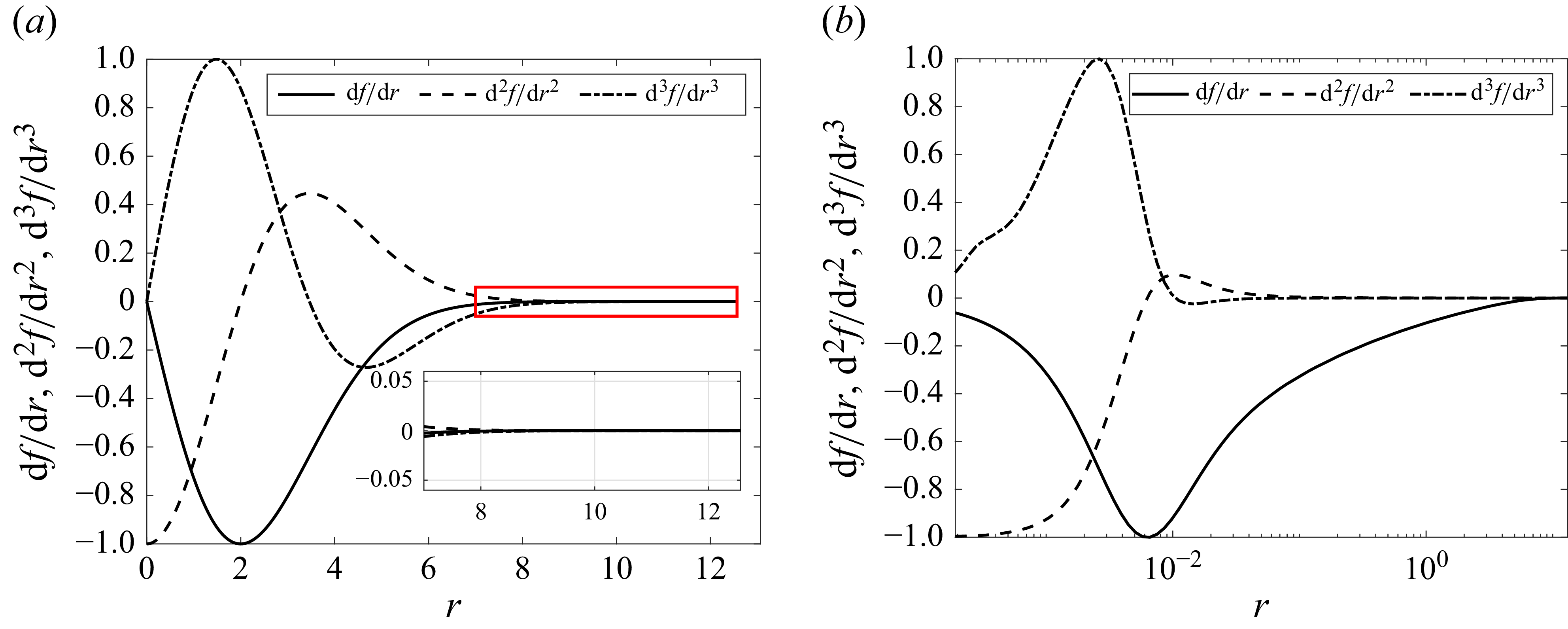

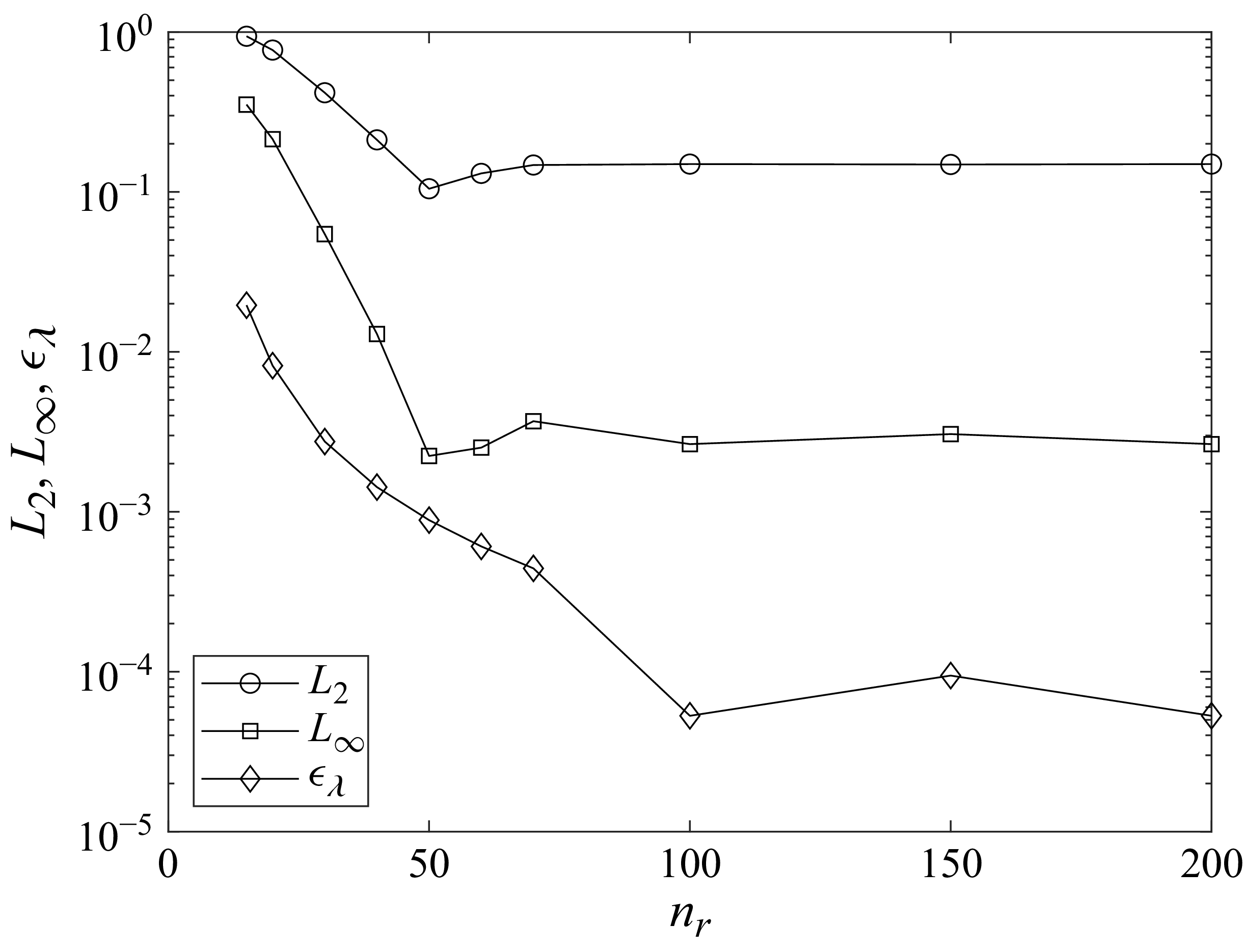


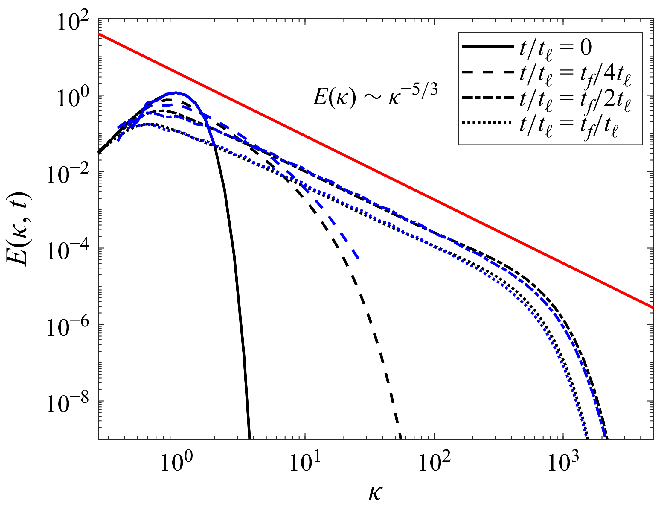


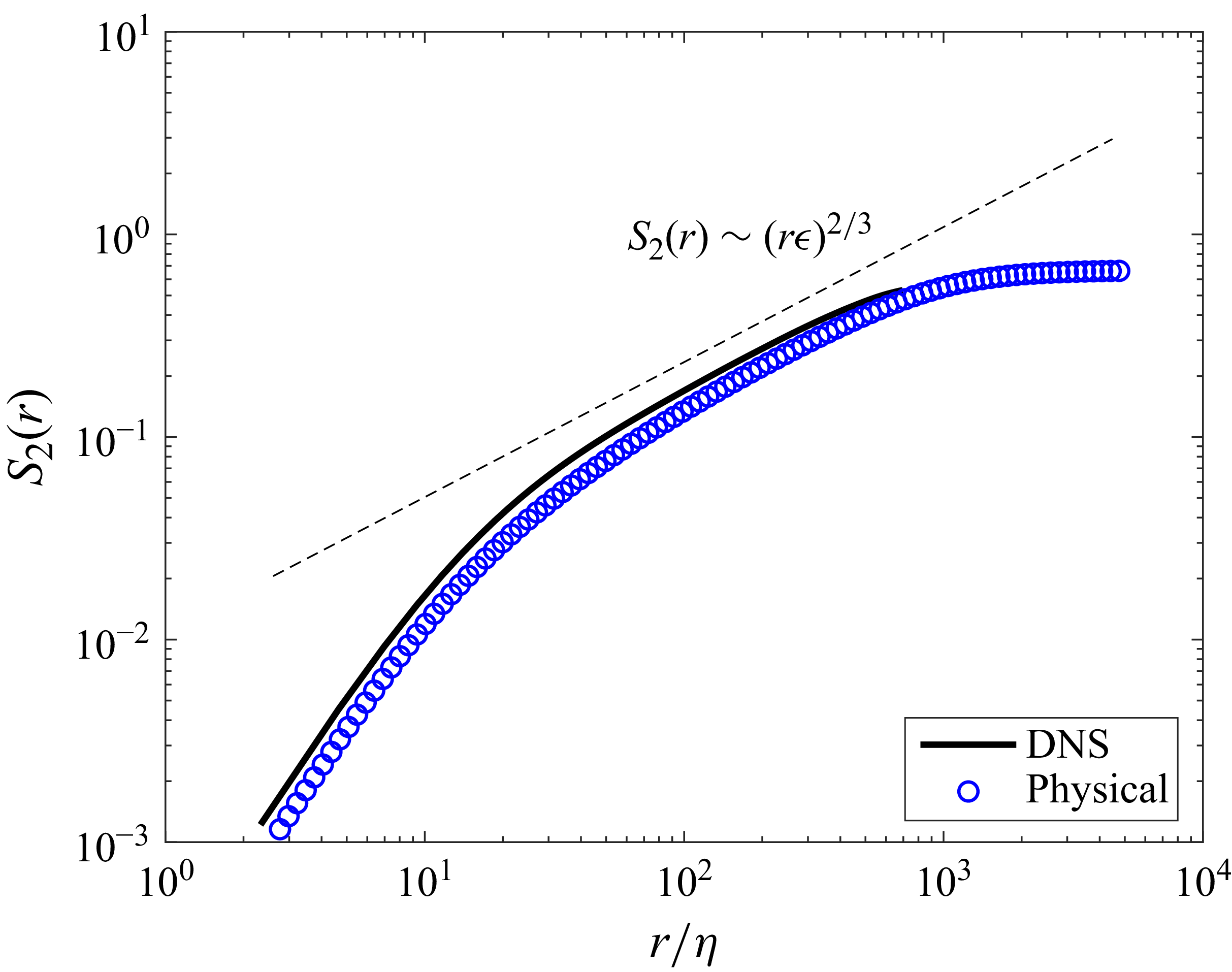


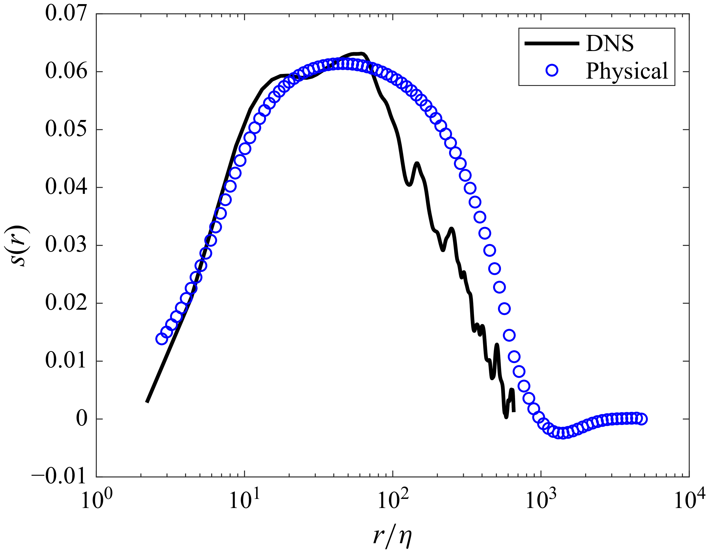


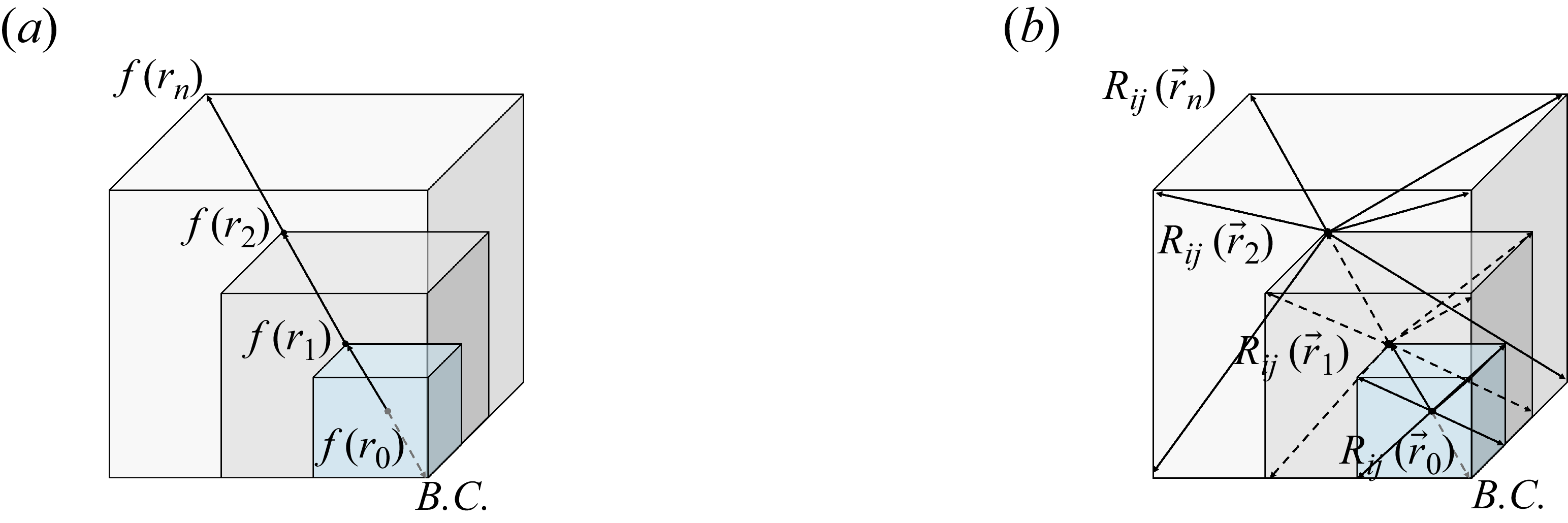
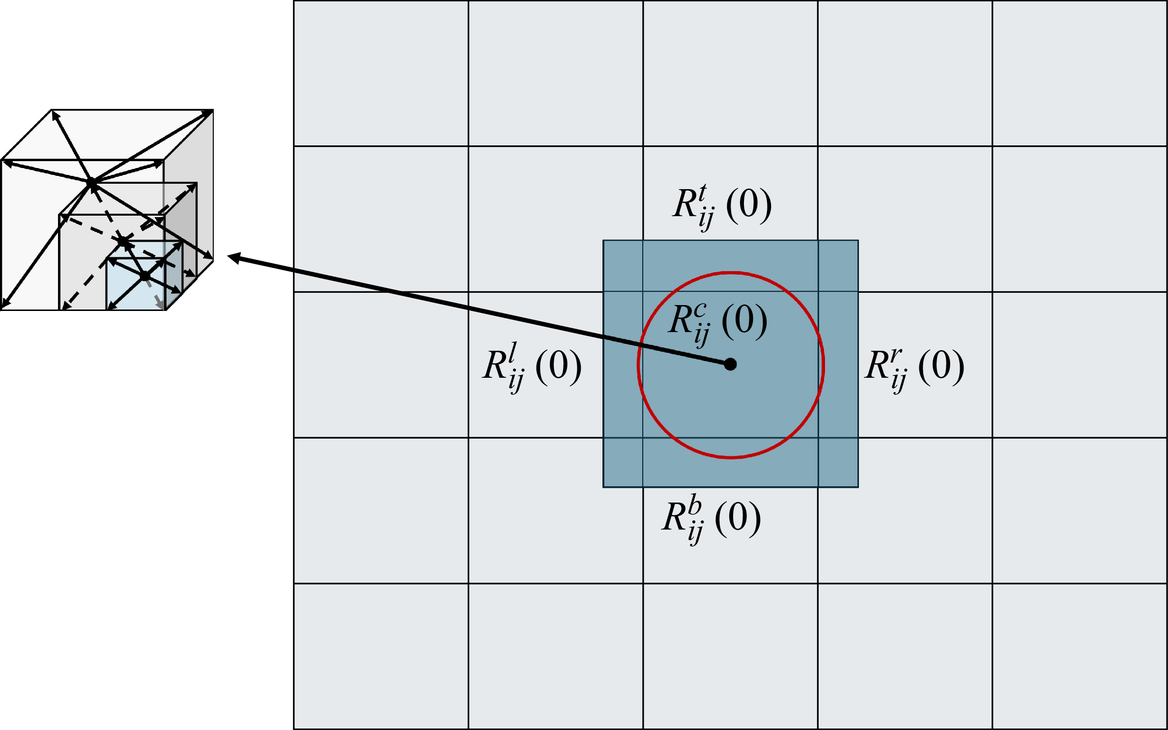

 Open access