


1. Introduction
Large-eddy simulation (LES) is a technique in which large-scale turbulent motions are directly resolved on the computational grid while the effect of filtered subgrid-scale (SGS) turbulent motions are modelled using an SGS model. In order to model the dissipative nature of the SGS stress tensor, which is known to be the essential component of the SGS modelling (Liu, Meneveau & Katz Reference Liu, Meneveau and Katz1994), eddy-viscosity SGS models are often utilised (Smagorinsky Reference Smagorinsky1963; Lilly Reference Lilly1967; Germano et al. Reference Germano, Piomelli, Moin and Cabot1991; Vreman Reference Vreman2004; Silvis, Remmerswaal & Verstappen Reference Silvis, Remmerswaal and Verstappen2017). In eddy-viscosity SGS models the deviatoric part of the SGS stress tensor  $\tau _{ij}$ is modelled as an algebraic function of the resolved strain-rate tensor $\bar {S}_{ij}$ such that $\tau _{ij} - \frac {1}{3}\tau _{kk}\delta _{ij} = - 2\nu _t \bar {S}_{ij}$, where $\overline {(\,{\cdot }\,)}$ denotes the spatial filter operation, $S_{ij}$ is the strain-rate tensor, $\delta _{ij}$ is the Kronecker delta and $\nu _t$ denotes the eddy viscosity (Silvis et al. Reference Silvis, Remmerswaal and Verstappen2017). While $\nu _t$ is modelled as $C\varPi ^g$, where $C$ and $\varPi ^g$ are the model coefficient and the SGS kernel at the grid-filter level, respectively, the dynamic procedure developed by Germano et al. (Reference Germano, Piomelli, Moin and Cabot1991) enabled dynamic determination of $C$.
$C$.
However, eddy-viscosity SGS models have the shortcoming that they correlate poorly with the true SGS stress tensor since eddy-viscosity models are aligned with  $\bar {S}_{ij}$ (Bardina, Ferziger & Reynolds Reference Bardina, Ferziger and Reynolds1983; Anderson & Meneveau Reference Anderson and Meneveau1999; da Silva & Métais Reference da Silva and Métais2002) and are not able to predict backscatter to the resolved scales (Zang, Street & Koseff Reference Zang, Street and Koseff1993). To alleviate the problems, various mixed SGS models that combine eddy-viscosity models with the modified Leonard term (Zang et al. Reference Zang, Street and Koseff1993; Bardina et al. Reference Bardina, Ferziger and Reynolds1983; Germano Reference Germano1986), the resolved stress $L_{ij} (=\widehat {\bar {u}_i\bar {u}_j}-\hat {\bar {u}}_i\hat {\bar {u}}_j)$ (Anderson & Meneveau Reference Anderson and Meneveau1999; Liu et al. Reference Liu, Meneveau and Katz1994) and the Clark model (Anderson & Meneveau Reference Anderson and Meneveau1999) were proposed. The dynamic procedure (Germano et al. Reference Germano, Piomelli, Moin and Cabot1991) was also applied to one-parameter (Zang et al. Reference Zang, Street and Koseff1993) and two-parameter (Liu et al. Reference Liu, Meneveau and Katz1994; Salvetti & Banerjee Reference Salvetti and Banerjee1995; Anderson & Meneveau Reference Anderson and Meneveau1999) mixed models, where the parameter refers to the model coefficients. Although dynamic mixed models are reported to exhibit smaller fluctuations in model coefficients, dynamic eddy-viscosity models and dynamic mixed models require ad hoc procedures such as averaging of model coefficients in statistically homogeneous directions and clipping of negative model coefficients (Zang et al. Reference Zang, Street and Koseff1993; Salvetti & Banerjee Reference Salvetti and Banerjee1995) to avoid numerical instability. Despite this issue, dynamic eddy-viscosity and dynamic mixed models have been successfully applied to various turbulent flows (Germano et al. Reference Germano, Piomelli, Moin and Cabot1991; Zang et al. Reference Zang, Street and Koseff1993; Salvetti & Banerjee Reference Salvetti and Banerjee1995; Anderson & Meneveau Reference Anderson and Meneveau1999; Vreman Reference Vreman2004; Silvis et al. Reference Silvis, Remmerswaal and Verstappen2017).
Recently, there have been studies to develop SGS models using an artificial neural network (ANN) (Wang et al. Reference Wang, Luo, Li, Tan and Fan2018; Xie & Wang Reference Xie and Wang2019; Xie et al. Reference Xie, Li, Ma and Wang2019; Xie, Wang & Weinan Reference Xie, Wang and Weinan2020a; Xie, Yuan & Wang Reference Xie, Yuan and Wang2020b; Yuan, Xie & Wang Reference Yuan, Xie and Wang2020). An ANN constructs a nonlinear mapping between a set of resolved flow variables and unresolved SGS stress using a series of matrix multiplications and nonlinear activation functions, while the conventional models represent the SGS stress in an algebraic function of resolved flow variables. As a result, ANN-based models are often expected to provide a more accurate flow description than algebraic dynamic SGS models (Xie & Wang Reference Xie and Wang2019; Xie et al. Reference Xie, Li, Ma and Wang2019, Reference Xie, Wang and Weinan2020a). For instance, Xie et al. (Reference Xie, Wang and Weinan2020a) showed from an a posteriori test of forced homogeneous isotropic turbulence that their ANN-based model predicted the energy spectrum and probability density functions (p.d.f.s) of the vorticity and velocity increment more accurately than the dynamic Smagorinsky model (DSM) and the dynamic mixed model. The ANN-based SGS models (hereafter ANN-SGS models) are also often known to be free from ad hoc procedures such as averaging and clipping of model coefficients for a certain set of input variables, which will be discussed later (Wang et al. Reference Wang, Luo, Li, Tan and Fan2018; Xie & Wang Reference Xie and Wang2019; Xie et al. Reference Xie, Li, Ma and Wang2019, Reference Xie, Wang and Weinan2020a,Reference Xie, Yuan and Wangb; Yuan et al. Reference Yuan, Xie and Wang2020). Therefore, ANN-SGS models have the potential to be not only free from the requirement of a statistically homogeneous direction but also provide improved prediction of the SGS stress.
Despite such potentially favourable features, ANN-SGS models raise three issues. The first issue is that although the performance of ANN-based models is known to be sensitive to the types of variables and the number of data points used for inputs, there is still no general consensus on which input variables and how many data points for each input variable are appropriate (Wang et al. Reference Wang, Luo, Li, Tan and Fan2018; Xie & Wang Reference Xie and Wang2019; Xie et al. Reference Xie, Li, Ma and Wang2019, Reference Xie, Wang and Weinan2020a; Park & Choi Reference Park and Choi2021). Wang et al. (Reference Wang, Luo, Li, Tan and Fan2018) performed an a priori study of decaying homogeneous isotropic turbulence to test the utility of single-point input variables such as the filtered velocity vector  $\bar {u}_i$, the velocity gradient tensor $\partial \bar {u}_i/\partial x_j$ and the second-order velocity derivative $\partial ^2\bar {u}_i/(\partial x_j \partial x_k)$. They found that $\partial \bar {u}_i/\partial x_j$ and $\bar {u}_i$ were the most and least important, respectively, for predictive accuracy. Xie et al. (Reference Xie, Wang and Weinan2020a) found that the multi-point input $\partial \bar {u}_i/\partial x_j$ led to higher correlation coefficients between the true and predicted SGS stresses than the single-point input $\partial \bar {u}_i/\partial x_j$ from an a priori study of forced homogeneous isotropic turbulence.
Park & Choi (Reference Park and Choi2021), on the other hand, tested both single-point and multi-point resolved strain-rate tensors  $\bar {S}_{ij}$ and $\partial \bar {u}_i/\partial x_j$ as inputs for ANN-based LES of a turbulent channel flow and found from an a posteriori test that the use of multi-point inputs required backscatter clipping due to numerical instabilities, while the use of single point $\bar {S}_{ij}$ resulted in the best performance. These are interesting results because, firstly, the use of a single-point input was essential for numerical stability, at least in the case of near-wall turbulence; secondly, the elaborate selection of input variables such as $\bar {S}_{ij}$ led to a better performance of ANN-SGS models than the use of general input variables such as $\bar {u}_i$ or $\partial \bar {u}_i/\partial x_j$.
Based on the knowledge from the algebraic SGS modelling in the framework of mixed modelling and from the recent reports on the selection of input variables and the number of input points, it is expected that an improved ANN-SGS model can be designed. For example, the drawback associated with misalignment of the SGS stress tensor can be overcome in a numerically stable manner by forming an ANN-based mixed model that utilises both the resolved strain-rate tensor and the resolved stress  $L_{ij} (=\widehat {\bar {u}_i\bar {u}_j}-\hat {\bar {u}}_i\hat {\bar {u}}_j)$ (Liu et al. Reference Liu, Meneveau and Katz1994; Anderson & Meneveau Reference Anderson and Meneveau1999) as inputs at a single point.
The second issue for ANN-based models is the generalization to untrained flow conditions, untrained grid resolution, and untrained types of flow. A few studies have reported application of an ANN-based model that was trained for a certain flow at low Reynolds numbers to the same flow at untrained higher Reynolds numbers (Maulik et al. Reference Maulik, San, Rasheed and Vedula2018, Reference Maulik, San, Rasheed and Vedula2019; Park & Choi Reference Park and Choi2021). However, generalization to flow on an untrained grid resolution has not been successful. Park & Choi (Reference Park and Choi2021) reported that an ANN-based model trained at a certain grid resolution did not accurately predict the turbulent statistics on untrained coarser or finer resolution, while it was possible to predict flow on an untrained grid resolution when the network was trained on coarser and finer resolution than the target resolution. Similarly, Zhou et al. (Reference Zhou, He, Wang and Jin2019) reported that predicting turbulent flow on a different grid resolution was difficult using an ANN-based model trained on other than the target grid resolution.
Most studies on ANN-based models addressed application of an ANN trained for a particular type of flow to the same type of flow. Although Xie et al. (Reference Xie, Wang and Weinan2020a,Reference Xie, Yuan and Wangb) briefly discussed application of ANN-based models trained with forced homogeneous isotropic turbulence to weakly compressible homogeneous shear flow, both flows are statistically stationary at the same Reynolds number and on the same grid resolution. Therefore, it is important to identify conditions of inputs and outputs of an ANN to achieve better generalization to flow on a different grid resolution and eventually to a different type of flow from trained flows.
The last issue is that the computational cost of ANN-based models has been reported to be higher than that of the algebraic dynamic eddy-viscosity and the dynamic mixed models. Park & Choi (Reference Park and Choi2021), Wang et al. (Reference Wang, Luo, Li, Tan and Fan2018), Yuan et al. (Reference Yuan, Xie and Wang2020), Xie & Wang (Reference Xie and Wang2019) and Xie et al. (Reference Xie, Wang and Weinan2020a) reported  $1.3$, $1.8$, $2.4$, $15$ and $256$ times higher computational cost than that of the DSM for simulations of turbulent channel flow (Park & Choi Reference Park and Choi2021) and homogeneous isotropic turbulence (Wang et al. Reference Wang, Luo, Li, Tan and Fan2018; Xie & Wang Reference Xie and Wang2019; Xie et al. Reference Xie, Wang and Weinan2020a; Yuan et al. Reference Yuan, Xie and Wang2020), respectively. Yuan et al. (Reference Yuan, Xie and Wang2020), Xie & Wang (Reference Xie and Wang2019) and Xie et al. (Reference Xie, Wang and Weinan2020a) also reported that the computational cost of their ANN-based models is higher than that of the dynamic mixed model (Anderson & Meneveau Reference Anderson and Meneveau1999). To make ANN-SGS models be practical, both accuracy and computational efficiency that are superior to those of the conventional algebraic SGS models should be achieved.
The primary objective of the present study is to develop a new ANN-based mixed SGS model that predicts the SGS stress tensor more accurately and stably. Analogously to the philosophy of the algebraic mixed SGS models, the present model is designed to consider both the resolved stress and strain-rate tensors as inputs and thereby produce the SGS stress associated with both the inputs as an output. The new model is also designed to be applicable to turbulent flow at untrained Reynolds numbers and on an untrained grid resolution, and, at the same time, to be computationally more efficient than the conventional algebraic SGS models. As noted by Park & Choi (Reference Park and Choi2021), the numerical stability is sought by conducting the input–output data sampling on a single grid point. The single-point data sampling is also beneficial in minimizing the computational cost. To achieve the goal, extensive analyses for finding optimal input–output scalings are conducted through a priori and a posteriori tests of homogeneous isotropic turbulence. The predictive capability, accuracy and stability of the ANN-based mixed SGS model for LES of homogeneous isotropic turbulence at untrained Reynolds numbers as well as on an untrained grid resolution are evaluated in detail. The applicability to other types of turbulent flow, especially the wall-bounded turbulent flow is investigated by performing LES of a turbulent channel flow.
This paper is organised as follows. Numerical methods for direct numerical simulation (DNS), LES and ANN are presented in § 2. In § 3 the performance and the characteristics of ANN-SGS models with different input sets are discussed based on results of a priori and a posteriori tests of forced isotropic turbulence. Application of the present ANN-based mixed SGS model to decaying isotropic turbulence at untrained Reynolds numbers and on an untrained grid resolution and untrained turbulent channel flow are presented in § 3. Comparison of the predictive capability as well as the computational cost of the developed ANN-based mixed SGS model with those of algebraic dynamic mixed models are also discussed in § 3, followed by concluding remarks in § 4.
2. Numerical methods
2.1. Direct numerical simulation of forced homogeneous isotropic turbulence
The incompressible Navier–Stokes equations for DNS are
 $$\begin{gather} \frac{\partial{u_{i}}}{\partial{x_{i}}} = 0, \end{gather}$$
 $$\begin{gather}\frac{\partial{u_{i}}}{\partial{t}} + \frac{\partial{u_{i}u_{j}}}{\partial{x_{j}}} ={-}\frac{1}{\rho}\frac{\partial{p}}{\partial{x_{i}}} + \nu\frac{\partial^2{u_{i}}}{\partial{x_{j}}\partial{x_{j}}}, \end{gather}$$
where  $x_{i}$ $(=x,y,z)$ are the Cartesian coordinates, $u_{i}$ $(=u,v,w)$ are the corresponding velocity components, $t$ is time, $p$ is pressure, $\rho$ is density and $\nu$ is kinematic viscosity.
Forced homogeneous isotropic turbulence at  $Re_{\lambda }=106$, $164$ and $286$, which were simulated by Mohan, Fitzsimmons & Moser (Reference Mohan, Fitzsimmons and Moser2017), Langford & Moser (Reference Langford and Moser1999) and Chumakov (Reference Chumakov2008), respectively, are simulated in this study with the computational parameters shown in table 1. A pseudospectral code HIT3D (Chumakov Reference Chumakov2007, Reference Chumakov2008) is used to solve the incompressible Navier–Stokes equations in a periodic cubic box with the length of $2{\rm \pi}$ with $N$ grid points in each direction. Simulation results are quoted in arbitrary units (Yang & Lei Reference Yang and Lei1998; Langford & Moser Reference Langford and Moser1999; Meneguz & Reeks Reference Meneguz and Reeks2011) of each case (Langford & Moser Reference Langford and Moser1999; Chumakov Reference Chumakov2008; Mohan et al. Reference Mohan, Fitzsimmons and Moser2017) in which the domain size is $2{\rm \pi}$. A combination of spherical truncation and phase shifting (Canuto et al. Reference Canuto, Hussaini, Quarteroni and Zang1988) is used for dealiasing. The second-order Adams–Bashforth scheme is used for time integration (Kang & You Reference Kang and You2021).
Parameters for DNS of forced homogeneous isotropic turbulence. Here  $Re_{\lambda }$ is the Taylor-scale Reynolds number, $N$ is the number of grid points in each direction, $\nu$ is the viscosity, $\varepsilon _{p}$ is the prescribed dissipation rate, $k_f$ is the upper bound of the forcing wavenumber, $\eta$ is the Kolmogorov length scale and $k_{max}$ is the maximum resolved wavenumber.

The initial flow field of the Gaussian distribution and random phases is fully developed, and then instantaneous fields are sampled at every eddy turnover time. The number of samples  $N_S$ for each case is summarized in table 1. Validation of the present DNS is discussed in the following section.
2.2. Validation of DNS results
Mohan et al. (Reference Mohan, Fitzsimmons and Moser2017) and Langford & Moser (Reference Langford and Moser1999) used a negative viscosity forcing (Jiménez et al. Reference Jiménez, Wray, Saffman and Rogallo1993; Mohan et al. Reference Mohan, Fitzsimmons and Moser2017) for forced homogeneous isotropic turbulence at  $Re_{\lambda }=106$ and $164$, respectively, and Chumakov (Reference Chumakov2008) used a deterministic forcing (Machiels Reference Machiels1997) for forced homogeneous isotropic turbulence at $Re_{\lambda }=286$. The negative viscosity forcing is given as
 \begin{equation}
\hat{f}^V_{i}({\boldsymbol{k}},t) =
\left\{\begin{array}{@{}ll@{}} \varepsilon_{p}
\hat{u}_{i}|{\boldsymbol{k}}|^2({\boldsymbol{k}},t)/\left[2E^V_f(t)\right], & 0 < k \leqslant k_f ,\\ 0, & k_f < k, \end{array} \right.
\end{equation}
\begin{equation}
\hat{f}^V_{i}({\boldsymbol{k}},t) =
\left\{\begin{array}{@{}ll@{}} \varepsilon_{p}
\hat{u}_{i}|{\boldsymbol{k}}|^2({\boldsymbol{k}},t)/\left[2E^V_f(t)\right], & 0 < k \leqslant k_f ,\\ 0, & k_f < k, \end{array} \right.
\end{equation}
where  $\varepsilon _{p}$ denotes the prescribed mean dissipation rate, $k$ is the spherical wavenumber defined as $k=|\boldsymbol {k}|$, $k_f$ is the upper bound of the forcing wavenumber and $E^V_f(t)=\int _{0}^{k_f} |\boldsymbol {k}|^2 E(k,t)\,{\rm d}k$, where $E(k,t)$ is the energy spectrum at time $t$. The combined forcing and viscous term in the Fourier space becomes $-(\nu -\alpha )|\boldsymbol {k}|^2\hat {u}_{i}(\boldsymbol {k})$, where $\alpha = \varepsilon _{p}/[2E^V_f(t)]$. The deterministic forcing of Machiels (Reference Machiels1997) is given as
 \begin{equation} \hat{f}^M_{i}(\boldsymbol{k},t) = \left\{ \begin{array}{@{}ll@{}} \varepsilon_{p} \hat{u}_{i}(\boldsymbol{k},t)/\left[2E^M_f(t)\right], & 0 < k \leqslant k_f ,\\ 0, & k_f < k, \end{array} \right. \end{equation}
where  $E^M_f(t)=\int _{0}^{k_f} E(k,t)\,{\rm d}k$.
Three-dimensional energy spectra of forced homogeneous isotropic turbulence are compared with the reference DNS results in figure 1, except for the case at  $\textit {Re}_{\lambda }=106$ for which a reference energy spectrum is not available. The case at $\textit {Re}_{\lambda }=164$ is firstly simulated using the negative viscosity forcing following Langford & Moser (Reference Langford and Moser1999). The resulting energy spectrum shown in figure 1(b) exhibits an undershoot in the forcing wavenumber range. Another simulation at $\textit {Re}_{\lambda }=164$ with the deterministic forcing of Machiels, on the other hand, shows improved agreement with the reference DNS data in the forcing range. While the differences caused by the use of different forcing schemes are further discussed in Appendix A, DNS data obtained using the deterministic forcing of Machiels is used for analyses in the present study, as it better reproduces DNS results of Langford & Moser (Reference Langford and Moser1999). For the case of $\textit {Re}_{\lambda }=286$, a slight underprediction of the energy spectrum is observed and it is discussed in Appendix B to conclude that the present DNS is statistically well converged.
Energy spectra from DNS of forced homogeneous isotropic turbulence at (a)  $\textit {Re}_{\lambda }=106$, (b) $\textit {Re}_{\lambda }=164$ and (c) $\textit {Re}_{\lambda }=286$. The open circles, $\boldsymbol {\circ }$, represent DNS by (b) Langford & Moser (Reference Langford and Moser1999) and (c) Chumakov (Reference Chumakov2008); – - – (yellow orange dashed-dot line) represents the present DNS with the negative viscosity forcing; – – - (dark blue dashed line) represents the present DNS with the deterministic forcing of Machiels; —— (black line) represents the $k^{-5/3}$ line; vertical dashed lines indicate the grid-filter cutoff wavenumbers in the inertial subrange in which a priori tests are performed.

2.3. Large-eddy simulation and filter operations
By applying the spatial filter operation  $\overline {(\,{\cdot }\,)}$ to (2.1) and (2.2), the filtered Navier–Stokes equations for LES are obtained as
 $$\begin{gather} \frac{\partial{\bar{u}_{i}}}{\partial{x_{i}}} = 0, \end{gather}$$
 $$\begin{gather}\frac{\partial{\bar{u}_{i}}}{\partial{t}} + \frac{\partial{\bar{u}_{i}\bar{u}_{j}}}{\partial{x_{j}}} ={-}\frac{1}{\rho}\frac{\partial{\bar{p}}}{\partial{x_{i}}} + \nu\frac{\partial^2{\bar{u}_{i}}}{\partial{x_{j}}\partial{x_{j}}}-\frac{\partial{\tau_{ij}}}{ \partial{x_{j}}}, \end{gather}$$
where  $x_{i}$ $(=x,y,z)$ are the Cartesian coordinates, $\bar {u}_{i}$ $(=\bar {u},\bar {v},\bar {w})$ are the corresponding filtered velocity components, $t$ is time, $\bar {p}$ is filtered pressure, $\rho$ is density, $\nu$ is kinematic viscosity and $\tau _{ij} = \overline {u_{i}u_{j}}-\bar {u}_{i}\bar {u}_{j}$ is the SGS stress.
Low-pass spatial filter operations are defined at the grid- and test-filter levels. A grid-filter operation on a scalar variable  $\bar {\phi }$ is defined as
 \begin{equation} \bar{\phi}\left({\boldsymbol{x}}\right) = \int_{\varOmega} G\left({\boldsymbol{x}},\boldsymbol{\xi}\right) \phi\left(\boldsymbol{\xi}\right){\rm d}\boldsymbol{\xi}, \end{equation}
where  $\boldsymbol {x}$ and $\boldsymbol {\xi }$ are the spatial coordinate vectors in the flow domain of $\varOmega$. The filter kernel $G$ satisfies the normalisation condition and depends on the filter width defined as $\bar {\varDelta }$ for the grid filter. The filter width in three-dimensional space is calculated using the expression given by Deardorff (Reference Deardorff1970),
 \begin{equation} \varDelta=\sqrt[3]{\varDelta_1 \varDelta_2 \varDelta_3}, \end{equation}
where  $\varDelta _i$ denotes the filter width in the $i$ direction. In line with the definition of the grid filter in (2.7), a test-filter operator $\widehat {\overline {(\,{\cdot }\,)}}$ is similarly defined but with the test-filter width $\hat {\varDelta }$ instead of $\bar {\varDelta }$.
The filter-to-grid ratio is defined as  $\hat{\varDelta}/\bar {\varDelta }$, where $\hat{\varDelta}$ is the filter width associated with the filtering operator $\widehat {\overline {(\,{\cdot }\,)}}$. Since the Gaussian filter is adopted for both grid and test filters, the filter-to-grid ratio is set to $\sqrt {5}$ (Pope Reference Pope2001). Moreover, because the implicit numerical grid filter for a pseudospectral method is known to be the Fourier cutoff filter, the grid-filter width is chosen to be twice the grid spacing in order to approximate the Gaussian filter (Kang, Chester & Meneveau Reference Kang, Chester and Meneveau2003).
The Gaussian filter is chosen to be the representative of the graded filter of which the filter shape is similar to the implicit numerical filter shape of finite-difference and finite-volume methods that are more commonly used for simulations than the pseudospectral method. The reason for using the pseudospectral method in the present study is to minimize the effect of numerical errors. The top-hat filter also has been tested, but there are no considerable differences in the results.
2.4. Artificial neural network for SGS modelling
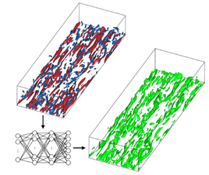
A fully connected neural network, also known as a multi-layer perceptron, is adopted in the present study. Six components of the SGS stress tensor  $\tau _{ij}$ are predicted by an ANN from a set of filtered input variables. The ANN is trained using input and output data from the filtered DNS (fDNS) fields, which are obtained by applying a spatial filter to the instantaneous fields from DNS of forced homogeneous isotropic turbulence in § 2.1. The filter width of the fDNS dataset is the same as the grid size of LES with $N^3=48^3$ cells at $Re_{\lambda } = 106$, and $N^3=128^3$ cells at $Re_{\lambda } = 286$. Through sufficient training, the ANN constructs a nonlinear mapping between a set of inputs and a target SGS stress tensor using a series of linear matrix multiplications and nonlinear activation functions. The mathematical operation from the $(n-1)$th layer to the $n$th layer takes the form of
 \begin{equation} X_{i}^{n} = \sigma \left ( \sum_{j} W_{ij}^{n} X_{j}^{n-1} + b_{i}^{n} \right), \end{equation}
where  $\sigma ({\cdot } )$ is the activation function, and $W_{ij}^{n}$ and $b_{i}^{n}$ are weights and biases, respectively. The output layer is linearly activated as $X_{i}^{N} = \sum _{j} W_{ij}^{N} X_{j}^{N-1} + b_{i}^{N}$, where $X_{i}^{N}$ is the output of the ANN.
The present ANN, which is shown in figure 2, consists of an input layer, 2 hidden layers with 12 neurons per hidden layer, and an output layer. Since the number of trainable parameters of an ANN directly affects its computational cost, a parameter study on the number of neurons per hidden layer is conducted in § 3.4. Based on the results in § 3.4, it is found that 12 neurons and 2 hidden layers are sufficient, and additional neurons or hidden layers do not improve the performance of the ANN. A Leaky–ReLu activation function ( $\sigma (x) = \max [-0.02x, x]$) is applied at each hidden layer. Leaky–ReLu is known to perform better than ReLu (Xu et al. Reference Xu, Wang, Chen and Li2015), as it is capable of resolving the gradient vanishing problem of the ReLu. During the training process, weights $W_{ij}^{n}$ and biases $b_{i}^{n}$ are optimised to minimise the mean-squared error loss function for six components of $\tau _{ij}$ defined as
 \begin{equation} {L} = \frac{1}{N_{batch}} \frac{1}{6} \sum_{n=1}^{N_{batch}} \sum_{j=1}^{3} \sum_{i=1}^{j} \left ( \tau_{ij,n}^{fDNS} - \tau_{ij,n} \right )^2, \end{equation}
where  $\tau _{ij}^{fDNS}$ and $\tau _{ij}$ are the true SGS stress obtained from fDNS and the predicted SGS stress, respectively. Mini-batch training is utilised in the present study and the iteration in figure 3 represents the mini-batch iteration. In each mini-batch iteration a subset of the training dataset (i.e. mini batch) is utilised to update the weights and biases of the ANN. Here $N_{batch}$ represents the size of the mini batch and is set to 128 (Park & Choi Reference Park and Choi2021).
Schematic diagram of the ANN to predict the SGS stress (two hidden layers and 12 neurons per hidden layer).

Learning curves of ANN-SGS models. Training and testing losses of (a) SL-106H, (b) SL-286H, (c)  $\text {SL-106}+286\text {H}$ and (d) S-106H. Coloured lines correspond to the training loss of each model, and black dashed-dot lines correspond to the testing loss of each model. The iteration in the horizontal axes represents the mini-batch iteration.

The sets of input and output variables and Reynolds numbers of the training datasets for ANN-SGS models are listed in table 2. Each ANN-SGS model is named such that the character and the number represent the input variables and the Reynolds number at which the ANN is trained, respectively. The character H at the end of the model names denotes homogeneous isotropic turbulence. For example, S-106H uses six components of  $\bar {S}_{ij}$ as inputs, whereas the other models use 12 components, six from $\bar {S}_{ij}$ and six from $L_{ij}$, as inputs. Effects of input variables on the characteristics and the accuracy of ANN-SGS models are discussed in § 3.1. In addition, the use of the resolved stress $L_{ij}$ among various scale-similarity terms is discussed in Appendix C. The ANN-SGS models are trained with fDNS datasets of forced homogeneous isotropic turbulence at the given Reynolds number.
Input variables and Reynolds numbers of training datasets for different ANN-SGS models.

The Adam optimiser with a learning rate of  $10^{-4}$ is utilised to optimise the trainable parameters. The ANN-SGS models listed in table 2 are trained for $5 \times 10^5$ iterations using the Python library PyTorch (Paszke et al. Reference Paszke, Gross, Chintala, Chanan, Yang, DeVito, Lin, Desmaison, Antiga and Lerer2017). A total of $2\times 10^{8}$ data points sampled from 30 snapshots of fDNS results are used for the training, whereas the rest are used for testing (80 % of the snapshots for training and 20 % for testing). Figure 3 shows the learning curve of the ANN-SGS models. The training loss and the testing loss show similar values and converge to a stationary value, indicating that all ANN-SGS models are trained without overfitting.
The performance of an ANN is highly affected by the normalisation of the input and output variables (Sola & Sevilla Reference Sola and Sevilla1997). In the present study, the input and the output tensors are normalised as  $\bar {S}_{ij}^* = \bar {S}_{ij}/\langle | \bar {S} |\rangle, L_{ij}^* = L_{ij}/\langle | L |\rangle$ and $\tau _{ij}^* = \tau _{ij}/\langle | \tau |\rangle$, where $\langle {\cdot } \rangle$ and $| {\cdot } |$ denote a volume average and an $L_2$ norm of the tensor, respectively. However, since the denominator $\langle | \tau |\rangle$ is unknown in actual LES, the normalisation factor for the SGS stress should be estimated. A detailed discussion regarding the normalisation factor for the SGS stress, particularly in the context of generalization to untrained conditions, is presented in § 3.2.
3. Results and discussion
In § 3.1 the performance of S-106H is compared with that of DSM from a priori and a posteriori tests of forced isotropic turbulence at  $Re_{\lambda } = 106$. Based on the above results, S-106H is improved by providing an additional input $L_{ij}$ (SL-106H). Accordingly, S-106H and SL-106H are compared in terms of the correlation coefficients, the p.d.f. of the SGS dissipation, the p.d.f. of the SGS stress and the energy spectrum. In § 3.2 special attention is given to the normalisation of the input and output tensors for the generalization of ANN-SGS models. Consequently, the generalizability of ANN-SGS models to transient flow is investigated in LES of decaying isotropic turbulence at various untrained conditions (i.e. initial Reynolds numbers and grid resolution). In §§ 3.3 and 3.4, the performance and the computational cost of the developed ANN-SGS models are compared with those of conventional algebraic dynamic mixed models. Finally, the application of the developed models to LES of turbulent channel flow is presented in §§ 3.5–3.7.
3.1. Effects of input variables: a priori and a posteriori tests
Before conducting an actual LES, the effects of input variables on ANN-SGS models are investigated in an a priori test of forced homogeneous isotropic turbulence at  $Re_{\lambda } = 106$. Although consistent predictive capability in the a priori and a posteriori tests is not always guaranteed (Park, Lee & Choi Reference Park, Lee and Choi2005; Park & Choi Reference Park and Choi2021), a priori tests are still considered to be a useful step for evaluating SGS models (Piomelli, Moin & Ferziger Reference Piomelli, Moin and Ferziger1988; Salvetti & Banerjee Reference Salvetti and Banerjee1995). It is also worth noting that the performance of ANN-SGS models are actually assessed in a posteriori tests in the present study. While the use of $\bar {S}_{ij}$ is expected to be preferable for homogeneous isotropic turbulence in terms of the accuracy and stability (Park & Choi Reference Park and Choi2021), it is of interest to investigate how differently the predicted SGS stress aligns with respect to $\bar {S}_{ij}$. To examine the alignment, the correlation coefficients between $\bar {S}_{ij}$ and the predicted SGS stress ( $\tau _{ij}^{ANN}$) are calculated and listed in table 3. The correlation coefficient between the components of arbitrary second-order tensors $\alpha _{ij}$ and $\beta _{ij}$ is defined as
 \begin{equation} Corr(\alpha_{ij},\beta_{ij}) = \frac{\left\langle \alpha_{ij} \beta_{ij} \right\rangle}{\left\langle \alpha_{ij}^2 \right\rangle^{1/2} \left\langle \beta_{ij}^2 \right\rangle^{1/2}}, \end{equation}
where  $\langle {\cdot } \rangle$ denotes the ensemble averaging. As shown in table 3, S-106H has much higher correlation coefficients between $\bar {S}_{ij}$ and $\tau _{ij}^{ANN}$ than fDNS with the value exceeding $-0.8$, which indicates that the predicted SGS stress is aligned closer to the strain-rate tensor rather than the true SGS stress.
Correlation coefficients ( $Corr(\bar {S}_{ij}, \tau _{ij})$) between $\bar {S}_{ij}$ and the predicted SGS stress by ANN-SGS models from an a priori test of forced homogeneous isotropic turbulence at $Re_{\lambda } = 106$.

Additionally, the p.d.f. of the SGS dissipation  $\varepsilon _{SGS}$ ( $= -\tau _{ij}\bar {S}_{ij}$) predicted by S-106H is shown in figure 4(a). Negative SGS dissipation corresponds to the backscatter, which is the kinetic energy transfer from the subgrid scale to the resolved scale. Interestingly, S-106H shows a similar characteristic to that of the eddy-viscosity models that are not capable of predicting backscatter. It can be considered that an ANN-SGS model that uses the resolved strain-rate tensor alone as the input only rescales the given input $\bar {S}_{ij}$ to predict the SGS stress while maintaining its alignment.
Results from an a priori test of forced homogeneous isotropic turbulence at  $Re_\lambda = 106$. (a) P.d.f. of the SGS dissipation $\varepsilon _{SGS}$ ( $= -\tau _{ij}\bar {S}_{ij}$); (b) p.d.f. of $\tau _{23}$. Here —— (thick black solid line), fDNS; —— (thick red solid line), SL-106H; – – - (thick green dashed line), S-106H.

Based on this observation, the performance of S-106H in actual LES is compared with that of DSM by conducting a posteriori tests of forced isotropic turbulence at  $Re_\lambda = 106$. The energy spectrum and p.d.f.s of the SGS dissipation and the SGS stress from S-106H are compared with those from DSM and fDNS. The SGS stress of DSM (Germano et al. Reference Germano, Piomelli, Moin and Cabot1991; Lilly Reference Lilly1992) is given as
 \begin{equation} \tau_{ij} - \tfrac{1}{3}\delta_{ij}\tau_{kk} ={-}2C\bar{\varDelta}^2|\bar{S}|\bar{S}_{ij}, \end{equation}
where  $|\bar {S}|=\sqrt {2\bar {S}_{ij} \bar {S}_{ij}}$, $\bar {S}_{ij}=\frac {1}{2}(\partial \bar {u}_i/\partial x_j+\partial \bar {u}_j/\partial x_i)$, $C=\langle L_{ij}M_{ij}\rangle /\langle M_{ij}M_{ij}\rangle$, $L_{ij}=\widehat {\bar {u}_i\bar {u}_j}-\hat {\bar {u}}_i\hat {\bar {u}}_j$, $M_{ij}=-2\hat {\varDelta }^2|\hat {\bar {S}}|\hat {\bar {S}}_{ij}+2\bar {\varDelta }^2|\widehat {\bar {S}|\bar {S}_{ij}}$, $\bar {\varDelta }$ and $\hat {\varDelta } (= \sqrt {5}\bar {\varDelta })$ are the grid-filter and test-filter scales, respectively. $\overline {(\,{\cdot }\,)}$ denotes the grid-level filter at $\bar {\varDelta }$ scale, $\widehat {(\,{\cdot }\,)}$ denotes the test filter at $\hat {\varDelta }$ scale and $\langle {\cdot } \rangle$ denotes averaging over homogeneous directions (volume averaging for homogeneous isotropic turbulence). The LES are performed using a pseudospectral code HIT3D (Chumakov Reference Chumakov2007, Reference Chumakov2008) with the dealiasing method of the $2/3$ rule. The second-order Adams–Bashforth scheme is used for time integration and the time step size is set so that the Courant–Friedrichs–Lewy number of LES is the same as that of DNS (Wang et al. Reference Wang, Luo, Li, Tan and Fan2018). The present ANN-SGS models predict the SGS stress tensor at each local grid point using resolved flow variables at the corresponding grid point as inputs. Large-eddy simulations with ANN-SGS models are performed without any ad hoc stabilisation procedures.
Figure 5 shows energy spectra from LES of forced isotropic turbulence at  $Re_\lambda = 106$ with a grid resolution of $48^3$, which is the same as that of the training data. The DSM is found to overestimate the energy spectrum in the range of $k \leqslant 5$. Interestingly, S-106H shows nearly identical performance to that of DSM in predicting the energy spectrum. In addition, from the p.d.f. of the SGS dissipation shown in figure 6(a), S-106H and DSM have the same characteristic that they are not capable of predicting backscatter. Note that the p.d.f. of the SGS stress ( $\tau _{23}$) predicted by S-106H is almost identical to that of DSM as both p.d.f.s are narrower than that of fDNS (figure 6b). This indicates that S-106H produces the SGS stress similar to that of DSM.
Energy spectra from fDNS and LES of forced homogeneous isotropic turbulence at  $Re_\lambda = 106$ with grid resolution of $48^3$. Here $\blacksquare$, fDNS; —— (thick black solid line), DSM; – – – (thick black dashed line), no-SGS; —— (thick red solid line), SL-106H; – – - (thick green dashed line), S-106H.

Results from an a posteriori test of forced homogeneous isotropic turbulence at  $Re_\lambda = 106$ with grid resolution of $48^3$. (a) P.d.f. of the SGS dissipation $\varepsilon _{SGS}$ ( $= -\tau _{ij}\bar {S}_{ij}$); (b) p.d.f. of $\tau _{23}$. Here $\blacksquare$, fDNS; —— (thick black solid line), DSM; —— (thick red solid line), SL-106H; – – - (thick green dashed line), S-106H.

From the above observation, it can be concluded that the ANN-SGS model with  $\bar {S}_{ij}$ as an input predicts the SGS stress that is closely aligned with the given input tensor, and performs similarly to DSM. Consequently, it is expected that S-106H can be improved by the similar concept employed in dynamic mixed models (Liu et al. Reference Liu, Meneveau and Katz1994; Anderson & Meneveau Reference Anderson and Meneveau1999). It is reported that a linear combination of the eddy-viscosity model with the resolved stress $L_{ij} (=\widehat {\bar {u}_i\bar {u}_j}-\widehat {\bar {u}}_i\hat {\bar {u}}_j)$ improves the accuracy of the predicted SGS stress with better alignment to the true SGS stress.
Similarly to the algebraic dynamic mixed models, it is expected that an ANN-SGS model can achieve closer alignment to the true SGS stress and more accurate prediction of the magnitude of the SGS stress if the resolved stress tensor  $L_{ij}$ is considered as an input in addition to the strain-rate tensor $\bar {S}_{ij}$ (i.e. ANN-SGS mixed model). A total of 12 components, six from $\bar {S}_{ij}$ and six from the resolved stress $L_{ij}$, are simultaneously provided as inputs for the ANN-SGS mixed model. To investigate the effect of the additional input variable, results of S-106H and SL-106H are compared in a priori and a posteriori tests of forced homogeneous isotropic turbulence at $Re_\lambda = 106$. Results of SL-106H are also compared with those of the algebraic dynamic mixed models in § 3.3.
The performance of SL-106H is compared with that of S-106H in an a priori test. The correlation coefficients between the true and the predicted SGS stress tensors are calculated following the definition of (3.1) and shown in table 4. The correlation coefficients of SL-106H are significantly improved compared with those of S-106H, which indicates that SL-106H reconstructs the instantaneous SGS stress closer to the true SGS stress. In table 3 the correlation coefficients between  $\bar {S}_{ij}$ and the predicted SGS stress $\tau _{ij}$ ( $Corr(\bar {S}_{ij}, \tau _{ij})$) from SL-106H are found to be closer to those of fDNS than those from S-106H, indicating that SL-106H is capable of aligning the principal axes of the predicted SGS stress closer to the true SGS stress. In addition, SL-106H provides excellent prediction of the p.d.f. of the SGS dissipation (figure 4a), which almost overlaps with that of fDNS. At the same time, SL-106H predicts the p.d.f. of the SGS stress ( $\tau _{23}$) closer to that of fDNS, whereas S-106H predicts a narrower p.d.f. as shown in figure 4(b).
Correlation coefficients ( $Corr(\tau _{ij}^{fDNS}, \tau _{ij}^{ANN})$) between the traceless parts of the true SGS stress ( $\tau _{ij}^{fDNS}$) and the predicted SGS stress by ANN-SGS models ( $\tau _{ij}^{ANN}$) from an a priori test of forced homogeneous isotropic turbulence at $Re_{\lambda } = 106$.

An a posteriori test of forced isotropic turbulence at  $Re_\lambda = 106$ is also conducted using SL-106H. As shown in figure 5, SL-106H predicts the energy spectrum closer to that of fDNS than S-106H and DSM in the range of $k \leqslant 5$. Furthermore, SL-106H noticeably better predicts the p.d.f. of the SGS dissipation than S-106H (figure 6a). It is worth noting that SL-106H is capable of accurately predicting the backscatter even in the a posteriori test; consequently, LES becomes stable without any ad hoc procedures, which is a clear advantage over the algebraic dynamic SGS models. Model SL-106H is found to predict the p.d.f. of the SGS stress ( $\tau _{23}$) more accurately, as shown in figure 6(b).
Figure 7 shows p.d.f.s of the resolved strain-rate tensor from fDNS and LES. Both SL-106H and DSM accurately predict the p.d.f. of  $\bar {S}_{11}$, while S-106H shows slight overestimation from the right tail of the p.d.f. On the other hand, no significant differences in the p.d.f.s of $\bar {S}_{23}$ from DSM, SL-106H and S-106H are observed.
The p.d.f.s of the resolved strain-rate tensor (a)  $\bar {S}_{11}$ and (b) $\bar {S}_{23}$ from an a posteriori test of forced homogeneous isotropic turbulence at $Re_\lambda = 106$ with grid resolution of $48^3$. Here $\blacksquare$, fDNS; —— (thick black solid line), DSM; —— (thick red solid line), SL-106H; – – - (thick green dashed line), S-106H.

Contours of the SGS dissipation ( $\varepsilon _{SGS}$) from fDNS and LES are shown in figure 8 for qualitative comparison. Snapshots are sampled after 21.5 large-eddy turnover times and at the centre of the domain in the $z$ direction. The SGS dissipation of SL-106H shows a relatively closer spatial distribution to that of fDNS than those of DSM and S-106H, since the backscatter (i.e. negative regions in the contours) is observed in the contours of SL-106H and fDNS, while DSM and S-106H are not capable of predicting the backscatter. This result is consistent with the p.d.f.s in figure 6(a).
Contours of the SGS dissipation  $\varepsilon _{SGS}$ ( $= -\tau _{ij}\bar {S}_{ij}$) from an a posteriori test of forced homogeneous isotropic turbulence at $Re_\lambda = 106$ with grid resolution of $48^3$. Results are shown for (a) fDNS, (b) DSM, (c) SL-106H, (d) S-106H.

The second-order longitudinal velocity structure functions from fDNS and LES of forced homogeneous isotropic turbulence at  $Re_\lambda = 106$ with a grid resolution of $24^3$, $48^3$ and $96^3$ are compared in figure 9. Note that SL-106H and S-106H are trained only for fDNS data with the filter size for $48^3$ resolution. Generalization to untrained resolution will be discussed in § 3.2. The second-order longitudinal velocity structure function $S_2^L(r)$ is defined as
 \begin{equation} S_2^L(r) \equiv \left\langle (\Delta u^L)^2 \right\rangle, \quad \Delta u^L \equiv \left[\boldsymbol{\bar{u}}(\boldsymbol{x}+\boldsymbol{r}) - \bar{\boldsymbol{u}}(\boldsymbol{x})\right]\boldsymbol{\cdot} \hat{\boldsymbol{r}}, \end{equation}
where  $\bar {\boldsymbol {u}}(\boldsymbol {x})$ is the filtered velocity vector at $\boldsymbol {x}$, $\hat {\boldsymbol {r}} = \boldsymbol {r}/|\boldsymbol {r}|$ is a unit vector in the direction of the separation $\boldsymbol {r}$. No distinctive differences in the structure functions at small separations are observed except for those of the no-SGS case that shows notable errors at small separations, indicating an inaccurate prediction of small-scale fluctuations. For all tested grid resolutions, SL-106H shows a more accurate prediction of the structure functions at large separations than DSM and S-106H.
The second-order longitudinal velocity structure functions  $S_2^L(r)$ from fDNS and LES of forced homogeneous isotropic turbulence at $Re_\lambda = 106$ with a grid resolution of (a) $24^3$, (b) $48^3$ and (c) $96^3$. The domain size $2{\rm \pi}$ is denoted by $L$. Here $\blacksquare$, fDNS; —— (thick black solid line), DSM; – – - (thick black dashed line), no-SGS; —— (thick red solid line), SL-106H; – – - (thick green dashed line), S-106H.

Results of a priori and a posteriori tests using SL-106H clearly indicate that considering the resolved stress  $L_{ij}$ as an input in addition to $\bar {S}_{ij}$ improves the performance of the ANN-SGS model. Unlike the SGS stress predicted by S-106H that is closely aligned with the given input $\bar {S}_{ij}$, the SGS stress predicted by SL-106H is closely aligned with the true SGS stress. Although the performance of S-106H is almost identical to that of DSM, both S-106H and SL-106H have advantages over DSM as they are free from the requirement of a stabilisation process such as averaging over statistically homogeneous directions or clipping of the negative model coefficients.
3.2. Generalization to untrained conditions: decaying homogeneous isotropic turbulence
In this section the application of ANN-SGS models trained with only forced homogeneous isotropic turbulence data to untrained decaying isotropic turbulence is discussed. For successful generalization to decaying isotropic turbulence, ANN-SGS models have to provide an accurate prediction of the SGS stress for various Reynolds numbers and grid resolution.
In this regard, normalisation of variables is important, as it plays a critical role for the consistent performance of an ANN under various conditions. As explained in § 2.4, the input and output tensors are normalised as 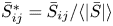 $\bar {S}_{ij}^* = \bar {S}_{ij}/\langle | \bar {S} |\rangle$, $L_{ij}^* = L_{ij}/\langle | L |\rangle$ and $\tau _{ij}^* = \tau _{ij}/\langle | \tau |\rangle$, where the denominator $\langle | \tau |\rangle$ requires an approximation in actual LES. The input variables ( $\bar {S}_{ij}$ and $L_{ij}$) are properly normalised by the magnitudes of the variables to have similar distributions for various conditions. However, normalising the SGS stress tensor to have similar distributions for various conditions is a challenging task because the approximation for $\langle | \tau |\rangle$ is not accurate enough. In other words, an inaccurate approximation of the normalisation factor of the output SGS stress results in a significantly different distribution of the normalised output for different conditions. In this situation, an ANN-based model could suffer from the prior probability shift issue, which occurs when the output variable distributions are different at training and test conditions (i.e. $P_{train}(y) \neq P_{test}(y)$, where $P(y)$ is a probability distribution of an output variable $y$) (Quiñonero-Candela et al. Reference Quiñonero-Candela, Sugiyama, Schwaighofer and Lawrence2009; Moreno-Torres et al. Reference Moreno-Torres, Raeder, Alaiz-Rodríguez, Chawla and Herrera2012). Dataset shift, including the prior probability shift, is not desirable for ANNs as it can cause significant changes in their performance during testing with untrained data (Gawlikowski et al. Reference Gawlikowski, Tassi, Ali, Lee, Humt, Feng, Kruspe, Triebel, Jung and Roscher2021). Consequently, the performance of an ANN-SGS model trained at a specific Reynolds number and on a certain grid resolution could be different from that at other flow conditions.
Therefore, it is suggested that a normalisation factor, which enables the distributions of the normalised inputs and outputs to remain unchanged for various Reynolds numbers and grid resolution, should be selected to avoid such performance inconsistency of an ANN-SGS model during the generalization. The modified Leonard term  $\mathcal {L}_{ij}^m$ ( $= \overline {\bar {u}_i \bar {u}_j} - \overline {\bar {u}}_i \overline {\bar {u}}_j)$, the resolved stress $L_{ij}$ ( $= \widehat {\bar {u}_i \bar {u}_j} - \hat {\bar {u}}_i \hat {\bar {u}}_j)$ and the gradient model term $\tau _{ij}^{grad}$ ( $= \frac {1}{12}\bar {\varDelta }^2({\partial \bar {u}_i}/{\partial x_k})({\partial \bar {u}_j}/{\partial x_k}))$ are considered to approximate the normalisation factor for the SGS stress. Among the three candidates, the term that has the most constant ratio to the true SGS stress $\langle | \tau |\rangle$ for various Reynolds numbers and grid resolution should be selected. Figure 10 shows ratios of $\langle | \tau ^{grad}|\rangle$, $\langle | \mathcal {L}^m |\rangle$ and $\langle | L |\rangle$ to $\langle | \tau ^{fDNS}|\rangle$, obtained at three different Reynolds numbers on a fixed grid resolution and three different grid resolutions at $Re_\lambda =106$. The gradient model term $\langle | \tau ^{grad}|\rangle$ shows the most constant ratio to the true SGS stress $\langle | \tau ^{fDNS}|\rangle$ for various Reynolds numbers and grid resolution, compared with the other two terms. Therefore, in the present study, the averaged $L_2$ norm of the gradient model term is selected to normalise and rescale the output SGS stress tensor as $\tau _{ij}^* = \tau _{ij}/\langle | \tau ^{grad}|\rangle$.
Ratios of  $\left \langle | \tau ^{grad}|\right \rangle$, $\left \langle | \mathcal {L}^m |\right \rangle$ and $\left \langle | L |\right \rangle$ to $\left \langle | \tau ^{fDNS}|\right \rangle$ at (a) $Re_{\lambda }=106$, 168 and 286 for $\bar {\varDelta }_{train}/\bar {\varDelta }=1$, and for (b) $\bar {\varDelta }_{train}/\bar {\varDelta }=1/2$, 1, 2 at $Re_{\lambda }=106$. Here —— (thick red solid line), $\left \langle | \tau ^{grad}|\right \rangle /\left \langle | \tau ^{fDNS}|\right \rangle$; —— (thick blue solid line), $\left \langle | \mathcal {L}^m |\right \rangle /\left \langle | \tau ^{fDNS}|\right \rangle$; —— (thick green solid line), $\left \langle | L |\right \rangle /\left \langle | \tau ^{fDNS}|\right \rangle$.

Figure 11 shows the p.d.f. of the SGS stress from fDNS of forced isotropic turbulence with and without normalisation. Distributions of the SGS stress without normalisation vary significantly depending on the Reynolds number and grid resolution, while the normalised SGS stress tensors show similar distributions for various Reynolds numbers and grid resolution, which enables an ANN-SGS model trained at a single condition to be successfully generalized to other conditions. In figure 12 effectiveness of the normalisation is verified in LES of forced homogeneous isotropic turbulence at  $Re_\lambda =106$ with a grid resolution of $24^3$ and $96^3$, which are coarser and finer by a factor of 2 than that of the training data, respectively. As shown in figure 12(a), SL-106H, SL-286H and $\text {SL-106}+286\text {H}$ predict the energy spectra more accurately than DSM and S-106H at all wavenumbers on a coarser resolution ( $24^3$). On a finer resolution of $96^3$, SL-106H, SL-286H and $\text {SL-106}+286\text {H}$ predict the energy spectra more accurately than DSM and S-106H in the range of $k \leqslant 6$ (figure 12b). This indicates that a proper choice of the normalisation factor for the output SGS stress enables the present ANN-SGS mixed models to perform accurately on an untrained coarser and finer grid resolution.
The p.d.f.s of the SGS stress  $\tau _{23}$ from fDNS of forced isotropic turbulence with various Reynolds numbers and grid resolution. (a) The p.d.f.s of $\tau _{23}$ without normalisation; (b) the p.d.f.s of normalised $\tau _{23}$ with $\langle | \tau ^{grad}|\rangle$. —— (thick black solid line), $Re_{\lambda }=106$, $\bar {\varDelta }_{train}/\bar {\varDelta }=1$; —— (thick red solid line), $Re_{\lambda }=106$, $\bar {\varDelta }_{train}/\bar {\varDelta }=1/2$; —— (thick blue solid line), $Re_{\lambda }=106$, $\bar {\varDelta }_{train}/\bar {\varDelta }=2$; —— (thick green solid line), $Re_{\lambda }=286$, $\bar {\varDelta }_{train}/\bar {\varDelta }=1$.

Energy spectra from fDNS and LES of forced homogeneous isotropic turbulence at  $Re_\lambda =106$ with a grid resolution of (a) $24^3$ and (b) $96^3$ (two-times coarser and finer resolution than that of training data, respectively). Here $\blacksquare$, fDNS; —— (thick black solid line), DSM; – – - (thick black dashed line), no-SGS; —— (thick red solid line), SL-106H; – – - (thick blue dashed line), SL-286H; – - – (thick yellow orange dashed-dot line), $\text {SL-106}+286{\rm H}$; – – – (thick green dashed line), S-106H.

Using  $\langle | \tau ^{grad}|\rangle$ as the normalisation factor, ANN-SGS models trained with only forced homogeneous isotropic turbulence data are applied to LES for decaying homogeneous isotropic turbulence to assess the generalizability to untrained transient flow. Table 5 shows the initial Reynolds numbers and grid resolution of test LES cases for decaying isotropic turbulence. The numerical methods are the same as those used for LES of forced isotropic turbulence. A fully converged instantaneous flow field of fDNS of forced homogeneous isotropic turbulence is selected as the initial field of decaying homogeneous isotropic turbulence. The robustness of ANN-SGS models to a random-phase initial condition is assessed in Appendix D.
Test LES cases for decaying homogeneous isotropic turbulence with ANN-SGS models and DSM. Here  $N$ is the number of grid points in each direction. Effects of grid resolution and the initial Reynolds number on the performance of ANN-SGS models are considered.

Figure 13 shows energy spectra from LES of decaying homogeneous isotropic turbulence at the initial Reynolds number  $Re_\lambda$ of 106 with a grid resolution of $48^3$. Energy spectra are obtained at $t/T_{e,0} = 1.1$, $3.3$ and $6.6$, where time $t$ is normalised by the initial eddy turnover time $T_{e,0}$. Energy spectra from S-106H and DSM are found to be almost identical. This is consistent with the a posteriori test of forced isotropic turbulence where S-106H performs similar to DSM. Both S-106H and DSM overestimate the energy spectra in the range of $k < 5$, and errors increase as flow evolves. In contrast, energy spectra from SL-106H, SL-286H and $\text {SL-106}+286\text {H}$ show better agreement with those of fDNS than DSM at all time steps.
Energy spectra from fDNS and LES of decaying homogeneous isotropic turbulence at the initial Reynolds number  $Re_\lambda$ of 106 with a grid resolution of $48^3$ (DHIT106 case). Results are shown for (a) $t/T_{e,0} = 1.1$; (b) $t/T_{e,0} = 3.3$; (c) $t/T_{e,0} = 6.6$. Here $\blacksquare$, fDNS; —— (thick black solid line), DSM; – – - (thick black dashed line), no-SGS; —— (thick red solid line), SL-106H; – – - (thick blue dashed line), SL-286H; – - – (thick yellow orange dashed-dot line), $\text {SL-106}+286\text {H}$; – – - (thick green dashed line), S-106H.

Additionally, temporal evolution of the resolved kinetic energy and the mean SGS dissipation are investigated from the same simulations and presented in figure 14. The DSM and S-106H predict smaller SGS dissipation than that of fDNS, which leads to a slower decaying rate of the resolved kinetic energy. Compared with DSM, SL-106H, SL-286H and  $\text {SL-106}+286\text {H}$ significantly better predict temporal evolutions of the resolved kinetic energy and the SGS dissipation, which are in good agreement with those of fDNS.
Results from fDNS and LES of decaying isotropic turbulence at the initial Reynolds number  $Re_\lambda$ of 106 with a grid resolution of $48^3$ (DHIT106 case). Temporal evolution of (a) the resolved kinetic energy and (b) the mean SGS dissipation $\langle \varepsilon _{SGS}\rangle$ ( $= \langle -\tau _{ij}\bar {S}_{ij}\rangle$) are shown. Here $\blacksquare$, fDNS; —— (thick black solid line), DSM; – – - (thick black dashed line), no-SGS; —— (thick red solid line), SL-106H; – – - (thick blue dashed line), SL-286H; – - – (thick yellow orange dashed-dot line), $\text {SL-106}+286\text {H}$; – – - (thick green dashed line), S-106H.

Similarly to the results of forced isotropic turbulence, SL-106H, SL-286H and  $\text {SL-106}+286\text {H}$ perform significantly better than DSM for LES of decaying isotropic turbulence, which clearly indicates that the additional input variable $L_{ij}$ is beneficial. In addition, SL-106H, SL-286H and $\text {SL-106}+286\text {H}$ provide stable solutions without any ad hoc stabilisation procedures unlike DSM during the temporal evolution of the flow.
Note that SL-106H, SL-286H and  $\text {SL-106}+286\text {H}$ show almost identical performance, although they are trained at different Reynolds numbers. This is because the present normalisation of the input and output variables enables the mapping of an ANN between the input resolved variables and the output SGS stress to remain unchanged for various flow conditions. Therefore, in the present study, training an ANN-SGS model at a single Reynolds number and on a single grid resolution is found to be sufficient for generalization to untrained flow conditions.
The performance of ANN-SGS models is further investigated through LES of decaying isotropic turbulence with different grid resolutions. Coarser ( $24^3$) and finer ( $96^3$) grid resolutions by a factor of 2 than that of the training dataset ( $48^3$) are considered. These are challenging cases, as the magnitudes of the SGS stress and the resolved kinetic energy differ from those of the training data as the turbulence decays. Nevertheless, SL-106H and SL-286H perform consistently better than DSM.
The LES of decaying homogeneous isotropic turbulence at the initial Reynolds number  $Re_\lambda$ of 106 with a grid resolution of $24^3$ is performed and results are shown in figure 15. The DSM and S-106H show similar performance; they overestimate the energy spectra at all wavenumbers, and the resolved kinetic energy decays slower than that of fDNS. On the other hand, SL-106H and SL-286H provide more accurate prediction of the energy spectra than that of DSM, especially with smaller errors at $k \leqslant 2$. Furthermore, SL-106H and SL-286H predict the temporal evolution of the resolved kinetic energy more accurately than DSM and S-106H.
Results from fDNS and LES of decaying isotropic turbulence at the initial Reynolds number  $Re_\lambda$ of 106 with a grid resolution of $24^3$ (DHIT106c case). (a) Energy spectra at $t/T_{e,0} = 1.1$, $3.3$ and $6.6$; (b) temporal evolution of the resolved kinetic energy. Here $\blacksquare$, fDNS; —— (thick black solid line), DSM; – – (thick black dashed line), no-SGS; —— (thick red dashed line), SL-106H; – – - (thick blue dashed line), SL-286H; – – - (thick green dashed line), S-106H.

Figure 16 shows results from LES of decaying homogeneous isotropic turbulence at the initial Reynolds number  $Re_\lambda$ of 106 with a grid resolution of $96^3$. As the grid resolution becomes finer, the energy spectra and the temporal evolution of the resolved kinetic energy obtained by SL-106H and SL-286H become more accurate and almost overlap with those of fDNS. However, DSM and S-106H overestimate energy spectra in the range of $k \leqslant 6$ and predict slower decaying rates of the resolved kinetic energy.
Results from fDNS and LES of decaying isotropic turbulence at the initial Reynolds number  $Re_\lambda$ of 106 with a grid resolution of $96^3$ (DHIT106f case). (a) Energy spectra at $t/T_{e,0} = 1.1$, $3.3$ and $6.6$; (b) temporal evolution of the resolved kinetic energy. Here $\blacksquare$, fDNS; —— (thick black solid line), DSM; – – - (thick black dashed line), no-SGS; —— (thick red solid line), SL-106H; – – - (thick blue dashed line), SL-286H; – – - (thick green dashed line), S-106H.

The performance of ANN-SGS models is tested through LES at a higher initial Reynolds number  $Re_\lambda$ of 286. Figure 17 shows results from LES of decaying homogeneous isotropic turbulence with a grid resolution of $128^3$, in which the cutoff wavenumber is located in the inertial range, same as in the training data. Notably, SL-106H is successfully generalized to the higher Reynolds number, and it predicts the energy spectra and the temporal evolution of the resolved kinetic energy more accurately than DSM. In figure 17(a), SL-106H and SL-286H accurately predict the energy spectra, which are in good agreement with those of fDNS. In contrast, DSM and S-106H slightly underestimate the energy at low wavenumbers ( $k \leqslant 2$), while they overestimated the energy at $4 \leqslant k \leqslant 10$. In figure 17(b) temporal evolutions of the resolved kinetic energy of SL-106H and SL-286H are well matched with those of fDNS at all time steps, whereas DSM and S-106H show slower decaying rates of the resolved kinetic energy until $t/T_{e,0} \approx 5$.
Results from fDNS and LES of decaying isotropic turbulence at the initial Reynolds number  $Re_\lambda$ of 286 with a grid resolution of $128^3$ (DHIT286 case). (a) Energy spectra at $t/T_{e,0} = 2.0$, $4.9$, $7.9$; (b) temporal evolution of the resolved kinetic energy. Here $\blacksquare$, fDNS; —— (thick black solid line), DSM; – – - (thick black dashed line), no-SGS; —— (thick red solid line), SL-106H; – – - (thick blue dashed line), SL-286H; – – - (thick green dashed line), S-106H.

Despite the fact that the present ANN-SGS models are not trained for the transient characteristics of decaying isotropic turbulence, they can be successfully utilised for LES of transient decaying isotropic turbulence with various initial Reynolds numbers and grid resolution. This is again possible due to the selection of proper normalisation factors for the input and output variables such that the normalisation enables the mapping of an ANN between the input resolved variables and the output SGS stress to remain unchanged during the temporal decay of turbulence.
It is worth noting that, for wall-bounded turbulent flow, normalisation of the SGS stress using the gradient model term may not be appropriate since it is known to have an incorrect near-wall scaling (Liu et al. Reference Liu, Meneveau and Katz1994). For turbulent channel flow and also for homogeneous isotropic turbulence, the magnitude of the resolved stress tensor is found to be the best alternative to the magnitude of the gradient model term. The advantage of using the resolved stress tensor for normalisation of the SGS stress over other normalisation options is discussed in Appendix E in detail.
3.3. Comparison with algebraic dynamic mixed models
In § 3.1 the predictive performance of SL-106H is found to meet the expectation that the use of both  $\bar {S}_{ij}$ and $L_{ij}$ as inputs could perform better than DSM due to better prediction of the SGS stress in terms of the magnitude and alignment to the true SGS stress. Consequently, it is of interest to investigate how well the ANN-SGS mixed model performs compared with the algebraic dynamic mixed models. Therefore, the performance of the developed ANN-SGS mixed model is compared with one-parameter (Zang et al. Reference Zang, Street and Koseff1993; Vreman, Geurts & Kuerten Reference Vreman, Geurts and Kuerten1994) and two-parameter (Anderson & Meneveau Reference Anderson and Meneveau1999) algebraic dynamic mixed models through LES of both forced and decaying isotropic turbulence.
The one-parameter dynamic mixed model that combines the eddy-viscosity model with the modified Leonard term  $(\mathcal {L}_{ij}^m = \overline {\bar {u}_i \bar {u}_j} - \bar {\bar {u}}_i \bar {\bar {u}}_j)$, which was formulated by Zang et al. (Reference Zang, Street and Koseff1993) and later modified by Vreman et al. (Reference Vreman, Geurts and Kuerten1994), is denoted as DMM. The model coefficient of DMM is dynamically determined to close the SGS stress as
 \begin{equation} \tau_{ij} - \tfrac{1}{3}\delta_{ij}\tau_{kk} ={-}2C\bar{\varDelta}^2|\bar{S}|\bar{S}_{ij} + \mathcal{L}_{ij}^m - \tfrac{1}{3}\delta_{ij}\mathcal{L}_{kk}^m, \end{equation}
where  $C=\left \langle M_{ij}(L_{ij}-H_{ij})\right \rangle /\left \langle M_{ij}M_{ij}\right \rangle$, $M_{ij}=-2\hat {\varDelta }^2|\hat {\bar {S}}|\hat {\bar {S}}_{ij}+2\bar {\varDelta }^2|\widehat {\bar {S}|\bar {S}_{ij}}$, $L_{ij}=\widehat {\bar {u}_i\bar {u}_j}-\hat {\bar {u}}_i\hat {\bar {u}}_j$, $H_{ij}=\widehat {\overline {\hat {\bar {u}}_i\hat {\bar {u}}_j}}-\hat{\bar{\hat{\bar{u}}_i}}\hat{\bar{\hat{\bar{u}}}_{j}}-(\widehat {\overline {\bar {u}_i\bar {u}_j}}- \widehat {\bar {\bar {u}}_i\bar {\bar {u}}_j})$, $\mathcal {L}_{ij}^m = \overline {\bar {u}_i \bar {u}_j} - \bar {\bar {u}}_i \bar {\bar {u}}_j$.
Anderson & Meneveau (Reference Anderson and Meneveau1999) formulated the dynamic two-parameter mixed model ( $DTM_{sim}$), which combines the eddy-viscosity model with the resolved stress and calculates two model coefficients for eddy-viscosity and mixed terms using the dynamic procedure as
 $$\begin{gather} \tau_{ij} ={-}2C_{1}\bar{\varDelta}^2|\bar{S}|\bar{S}_{ij} + C_{2}L_{ij}, \end{gather}$$
 $$\begin{gather}C_{1} = \frac{\left\langle L_{ij}M_{ij}\right\rangle \left\langle N_{ij}N_{ij}\right\rangle - \left\langle L_{ij}N_{ij}\right\rangle \left\langle M_{ij}N_{ij}\right\rangle }{\left\langle M_{ij}M_{ij}\right\rangle \left\langle N_{ij}N_{ij}\right\rangle - \left\langle N_{ij}M_{ij}\right\rangle ^2}, \end{gather}$$
 $$\begin{gather}C_{2} = \frac{\left\langle L_{ij}N_{ij}\right\rangle \left\langle M_{ij}M_{ij}\right\rangle - \left\langle L_{ij}M_{ij}\right\rangle \left\langle M_{ij}N_{ij}\right\rangle }{\left\langle M_{ij}M_{ij}\right\rangle \left\langle N_{ij}N_{ij}\right\rangle - \left\langle N_{ij}M_{ij}\right\rangle ^2}, \end{gather}$$
where  $L_{ij}=\widehat {\bar {u}_i\bar {u}_j}-\hat {\bar {u}}_i\hat {\bar {u}}_j$, $M_{ij}=-2\hat {\varDelta }^2|\hat {\bar {S}}|\hat {\bar {S}}_{ij}+2 \bar {\varDelta }^2|\widehat {\bar {S}|\bar {S}_{ij}}$, $N_{ij}=(\widetilde {\hat {\bar {u}}_i\hat {\bar {u}}_j}-\widetilde {\hat {\bar {u}}_i} \widetilde {\hat {\bar {u}}_j}) - (\widehat {\widehat {\bar {u}_i\bar {u}_j}}-\widehat {\hat {\bar {u}}_i\hat {\bar {u}}_j})$ and $\widetilde {(\,{\cdot }\,)}$ denotes the filtering at the $5\bar {\varDelta }$ scale.
Anderson & Meneveau (Reference Anderson and Meneveau1999) proposed another dynamic two-parameter mixed model ( $DTM_{nl}$), which combines the eddy-viscosity model with the Clark model as
 \begin{equation} \tau_{ij} ={-}2C_{1}\bar{\varDelta}^2|\bar{S}|\bar{S}_{ij} + C_{2}\bar{\varDelta}^2\frac{\partial \bar{u}_i}{\partial x_k}\frac{\partial \bar{u}_j}{\partial x_k}, \end{equation}
where  $C_{1}$ and $C_{2}$ are determined by (3.6) and (3.7), respectively, with $L_{ij}=\widehat {\bar {u}_i\bar {u}_j}-\hat {\bar {u}}_i\hat {\bar {u}}_j$, $M_{ij}=-2\hat {\varDelta }^2|\hat {\bar {S}}|\hat {\bar {S}}_{ij}+2\bar {\varDelta }^2| \widehat {\bar {S}|\bar {S}_{ij}}$, $N_{ij}=\hat {\varDelta }^2({\partial \hat {\bar {u}}_i}/{\partial x_k})({\partial \hat {\bar {u}}_j}/{\partial x_k}) - \bar {\Delta }^2\widehat { ( {\partial \bar {u}_i}/{\partial x_k} ) ({\partial \bar {u}_j}/{\partial x_k}) }$.
Table 6 shows correlation coefficients between the true and predicted SGS stresses by ANN-SGS models and algebraic SGS models from an a priori test of forced homogeneous isotropic turbulence at  $Re_{\lambda } = 106$. Model $DTM_{nl}$ shows the best correlation coefficients, while DSM shows the worst correlation coefficients among tested models with similar values to those reported by Xie et al. (Reference Xie, Yuan and Wang2020b). Correlation coefficients from $DTM_{sim}$ are better than those from DSM and worse than those from DMM (Salvetti & Banerjee Reference Salvetti and Banerjee1995; Xie et al. Reference Xie, Yuan and Wang2020b). Model S-106H shows poor correlation coefficients similar to DSM, while SL-106H shows comparable correlation coefficients to those of DMM. The p.d.f.s of the SGS stress $\tau _{23}$ in figure 18(b) show a similar trend. The DSM shows the most inaccurate p.d.f. of $\tau _{23}$, while $DTM_{sim}$ and SL-106H show similarly improved prediction. The DMM and $DTM_{nl}$ show more accurate p.d.f.s of the SGS stress compared with SL-106H. However, it is found from the following a posteriori test that higher correlation coefficients of the SGS stress in an a priori test do not guarantee more accurate LES results as also reported by Park et al. (Reference Park, Lee and Choi2005) and Park & Choi (Reference Park and Choi2021).
Results from an a priori test of forced homogeneous isotropic turbulence at  $Re_\lambda = 106$. (a) The p.d.f. of the SGS dissipation $\varepsilon _{SGS}$ ( $= -\tau _{ij}\bar {S}_{ij}$); (b) p.d.f. of $\tau _{23}$. Here $\blacksquare$, fDNS; —— (thick black solid line), DSM; – - – (thick black dashed-dot line), DMM; – - – (thick blue dashed-dot line), $DTM_{nl}$; – - – (thick green dashed-dot line), $DTM_{sim}$; —— (thick red solid line), SL-106H.

Correlation coefficients ( $Corr(\tau _{ij}^{fDNS}, \tau _{ij}^{model})$) between the traceless parts of the true SGS stress ( $\tau _{ij}^{fDNS}$) and the predicted SGS stress ( $\tau _{ij}^{model}$) from an a priori test of forced homogeneous isotropic turbulence at $Re_{\lambda } =106$.

Table 7 shows correlation coefficients between  $\bar {S}_{ij}$ and the predicted SGS stress $\tau _{ij}^{model}$. Model S-106H shows high absolute magnitudes of $Corr(\bar {S}_{ij}, \tau _{ij})$ similar to those of DSM, as discussed in § 3.1. Both DMM and $DTM_{nl}$ show closer values of $Corr(\bar {S}_{ij}, \tau _{ij})$ to those of fDNS compared with DSM. On the other hand, SL-106H predicts $Corr(\bar {S}_{ij}, \tau _{ij})$ most closely to those of fDNS. In addition, SL-106H shows the most accurate prediction of the p.d.f. of the SGS dissipation, while the dynamic mixed models overestimate the forward scatter (figure 18a). The DSM is not capable of predicting the backscatter.
Correlation coefficients ( $Corr(\bar {S}_{ij}, \tau _{ij})$) between $\bar {S}_{ij}$ and the predicted SGS stress from an a priori test of forced homogeneous isotropic turbulence at $Re_{\lambda } =106$.

Figure 19 shows energy spectra from LES of forced isotropic turbulence at  $Re_\lambda =106$ with a grid resolution of $48^3$, including those from the algebraic dynamic mixed models. Except for DSM, all models well predict the energy spectrum in the range of $k < 5$. However, energy spectra of DMM and $DTM_{sim}$ deviate from that of fDNS in the range of $k \geqslant 5$, showing large errors near the cutoff wavenumber. Model $DTM_{nl}$ accurately predicts the energy spectrum at all wavenumbers. Model SL-106H produces the energy spectrum nearly identical to that of $DTM_{nl}$. Both SL-106H and $DTM_{sim}$ accurately predict the SGS dissipation, whereas DSM and DMM underestimate the backscatter and $DTM_{nl}$ overestimates the forward scatter as shown in figure 20(b).
Energy spectra from fDNS and LES of forced homogeneous isotropic turbulence at  $Re_\lambda =106$ with a grid resolution of $48^3$. Here $\blacksquare$, fDNS; —— (thick black solid line), DSM; – - – (thick black dashed-dot line), DMM; – - – (thick blue dashed-dot line), $DTM_{nl}$; – - – (thick green dashed-dot line), $DTM_{sim}$; —— (thick red solid line), SL-106H.

The p.d.f. of the SGS dissipation  $\varepsilon _{SGS}$ from LES of forced homogeneous isotropic turbulence at $Re_\lambda =106$ with a grid resolution of $48^3$. (a) Without ad hoc stabilisation; (b) with ad hoc stabilisation including averaging of the model coefficients in statistically homogeneous directions and clipping of the negative model coefficients. Here $\blacksquare$, fDNS; —— (thick black solid line), DSM; – - – (thick black dashed-dot line), DMM; – - – (thick blue dashed-dot line), $DTM_{nl}$; – - – (thick green dashed-dot line), $DTM_{sim}$; —— (thick red solid line), SL-106H.

Note that the algebraic dynamic SGS models tested in the present study are stable only after applying ad hoc procedures (i.e. averaging of the model coefficients in statistically homogeneous directions and clipping of the negative model coefficients). A possible reason for this problem can be found from the p.d.f. of the SGS dissipation without ad hoc procedures, as shown in figure 20(a). The dynamic Smagorinsky and algebraic dynamic mixed models significantly overestimate both backscatter and forward scatter when the ad hoc procedures are not applied. The excessive backscatter causes LES to diverge within tens of time steps. In contrast, LES with SL-106H is stable without any ad hoc procedures, since SL-106H accurately predicts the p.d.f. of the SGS dissipation, which is a notable advantage of the present ANN-SGS mixed model.
Additionally, LES of decaying isotropic turbulence at the initial Reynolds number  $Re_\lambda$ of 106 with a grid resolution of $48^3$ is performed, and the results are shown in figures 21 and 22. Similarly to the results from LES of forced isotropic turbulence, DMM accurately predicts energy spectra at $k < 5$ but underpredicts the energy at $k \geqslant 5$. On the other hand, energy spectra of $DTM_{nl}$ are accurate at $k \geqslant 5$ but the energy of large scale at $k \leqslant 2$ is slightly overestimated at $t/T_{e,0} = 3.3$ and $6.6$. Model $DTM_{sim}$ provides similar energy spectra, resolved kinetic energy and SGS dissipation to those of DSM after $t/T_{e,0} \geqslant 1.62$ since the model coefficient $C_2$ of (3.5) becomes negative and is clipped as zero after that time. The same issue in decaying isotropic turbulence is reported by Anderson & Meneveau (Reference Anderson and Meneveau1999); the similarity coefficient of $DTM_{sim}$ becomes negative when the grid resolution is too coarse so that the test-filter size exceeds the integral scale. Compared with the algebraic dynamic mixed models, SL-106H predicts most accurately the energy spectra at all time steps; especially, it shows the smallest error in the range of $k < 5$. In addition, SL-106H most accurately predicts the temporal evolution of the resolved kinetic energy and the mean SGS dissipation, as shown in figure 22. This indicates that the present ANN-SGS mixed model with input tensors of $\bar {S}_{ij}$ and $L_{ij}$ is able to predict the decay of isotropic turbulence more accurately than the algebraic dynamic mixed models.
Energy spectra from fDNS and LES of decaying isotropic turbulence at the initial Reynolds number  $Re_\lambda =106$ with a grid resolution of $48^3$ (DHIT106 case). Results are shown for (a) $t/T_{e,0} = 1.1$; (b) $t/T_{e,0} = 3.3$; (c) $t/T_{e,0} = 6.6$. Here $\blacksquare$, fDNS; —— (thick black solid line), DSM; – - – (thick black dashed-dot line), DMM; – - – (thick blue dashed-dot line), $DTM_{nl}$; – - – (thick green dashed-dot line), $DTM_{sim}$; —— (thick red solid line), SL-106H.

Results from fDNS and LES of decaying isotropic turbulence at the initial Reynolds number  $Re_\lambda$ of 106 with a grid resolution of $48^3$ (DHIT106 case). Temporal evolution of (a) the resolved kinetic energy and (b) the mean SGS dissipation $\langle \varepsilon _{SGS}\rangle$ ( $= \langle -\tau _{ij}\bar {S}_{ij}\rangle$) are shown. Here $\blacksquare$, fDNS; —— (thick black solid line), DSM; – - – (thick black dashed-dot line), DMM; – - – (thick blue dashed-dot line), $DTM_{nl}$; – - – (thick green dashed-dot line), $DTM_{sim}$; —— (thick red solid line), SL-106H.

3.4. Computational cost of ANN-SGS models
Computational cost is an important factor of ANN-SGS models, as it is one of the main obstacles to the practical application of the models. Previous studies (Wang et al. Reference Wang, Luo, Li, Tan and Fan2018; Xie & Wang Reference Xie and Wang2019; Xie et al. Reference Xie, Wang and Weinan2020a; Yuan et al. Reference Yuan, Xie and Wang2020; Park & Choi Reference Park and Choi2021) reported that ANN-SGS models are computationally more expansive than DSM, which can be considered a major disadvantage. Therefore, a parameter study of the present ANN-SGS mixed model with the number of neurons per hidden layer is conducted to find an optimal size of the ANN, as the computational time for forward propagation of an ANN depends on the size of the ANN.
Five different ANNs with 12 to 48 neurons and 2 to 4 hidden layers are considered. The ANN-SGS mixed models with the five different ANNs are trained with the fDNS dataset of forced isotropic turbulence at  $Re_\lambda = 106$. Figure 23 shows results from LES of decaying homogeneous isotropic turbulence with a grid resolution of $48^3$ using ANN-SGS mixed models with ANNs of five different sizes. It is found that 12 neurons and 2 hidden layers are sufficient, and additional neurons or hidden layers do not improve the performance of the ANN-SGS mixed model. However, the computational time to evaluate the SGS stress increases with the number of neurons as ratios of ${\rm DSM} : 12n : 24n : 48n = 1 : 0.71 : 0.89 : 1.42$, where $n$ denotes the number of neurons per hidden layer. Therefore, in the present study an ANN with 12 neurons at each of the two hidden layers is selected.
Results from fDNS and LES of decaying isotropic turbulence at the initial Reynolds number  $Re_\lambda$ of 106 with a grid resolution of $48^3$. (a) Energy spectra at $t/T_{e,0} = 1.1$, $3.3$ and $6.6$; (b) temporal evolution of the resolved kinetic energy. Here $\blacksquare$, fDNS; ANN-SGS mixed model with —— (thick red solid line), 12 neurons and 2 hidden layers; – - – (thick yellow orange dashed-dot line), 24 neurons and 2 hidden layers; – - – (thick blue dashed-dot line), 48 neurons and 2 hidden layers; – – - (thick green dashed line), 12 neurons and 3 hidden layers; – – - (thick magenta dashed line), 12 neurons and 4 hidden layers.

The computational cost of the developed ANN-SGS mixed model is compared with those of the algebraic dynamic SGS models. For a fair comparison, the matrix operations of the ANN are implemented on the LES solver. The weight matrices and the bias vectors of the trained ANN are saved and transferred to the solver to perform a forward propagation of the ANN. All simulations are conducted using 16 CPU cores of Intel(R) Xeon(R) E5-2650 v2, and the time consumption for evaluating the SGS stress tensors during the same 100 time steps are compared. Figure 24 shows ratios of the computational time of the tested SGS models for evaluating the SGS stress. The algebraic dynamic mixed models require 1.6 to 2.2 times greater computational time than DSM to calculate the SGS stress. It is noteworthy that the developed ANN-SGS mixed model is computationally cheaper than the algebraic dynamic mixed models and even than DSM.
Ratio of computational time of tested SGS models for evaluating the SGS stress. Computational time is normalised to that of DSM.

3.5. Training and testing for turbulent channel flow
In this section application of the developed ANN-SGS mixed model to a wall-bounded flow is discussed. Turbulent channel flow at  $Re_{\tau }=180$ and 395 is considered. The predictive capabilities of the ANN-SGS mixed model that uses both $\bar {S}_{ij}$ and $L_{ij}$ as inputs and the ANN-SGS model with $\bar {S}_{ij}$ as the only input are investigated through a posteriori tests for a turbulent channel flow with various untrained Reynolds number and grid resolution. Additionally, it is further investigated whether the ANN-SGS mixed model trained with both channel flow and homogeneous isotropic turbulence at a certain condition is capable of providing accurate solutions for both types of flow at untrained conditions. Lastly, results from LES of turbulent channel flow with the ANN-SGS mixed model that is trained only with homogeneous isotropic turbulence are discussed.
Direct numerical simulations are performed with parameters summarized in table 8 to construct training datasets and reference solutions for LES. A fourth-order finite-difference code by Bose, Moin & You (Reference Bose, Moin and You2010) is utilised to conduct DNS and LES. The convection terms are discretized in a skew-symmetric form (Morinishi et al. Reference Morinishi, Lund, Vasilyev and Moin1998). A semi-implicit method is used for time marching. The viscous diffusion terms in the wall-normal direction are integrated implicitly with the Crank–Nicolson method, and the other terms are explicitly advanced with the third-order Runge–Kutta method (Morinishi et al. Reference Morinishi, Lund, Vasilyev and Moin1998; Bose et al. Reference Bose, Moin and You2010; Kang & You Reference Kang and You2021).
Parameters for DNS of turbulent channel flow. Here  $L_x$ and $L_z$ are the streamwise and spanwise domain sizes, respectively; $\delta$ is the channel half-width, and $N_x$, $N_y$ and $N_z$ are numbers of grid points in the streamwise, wall-normal, and spanwise directions, respectively; $\Delta x^+$ and $\Delta z^+$ are the streamwise and the spanwise grid sizes in wall units, respectively; $\Delta y_{min}^+$ and $\Delta y_{c}^+$ are the wall-normal grid sizes at the wall and the centreline, respectively.

The fDNS dataset of a turbulent channel flow at  $Re_{\tau } = 180$ is constructed by applying the grid and test filters with $\bar {\varDelta } = 4\varDelta _{DNS}$ and $\hat {\bar {\varDelta }} = 8\varDelta _{DNS}$ to instantaneous DNS fields, where $\varDelta _{DNS}$ is the grid spacing of DNS. The filter width $\bar {\varDelta }$ of the fDNS dataset is the same as the grid size of LES with $N_x\times N_y \times N_z = 48\times 48\times 48$ cells at $Re_{\tau }=180$. Fourth-order commutative discrete filters by Vasilyev, Lund & Moin (Reference Vasilyev, Lund and Moin1998) are utilised to construct the fDNS dataset and to conduct test filtering of LES. A total of $3.5\times 10^7$ data points are sampled from five instantaneous velocity fields of fDNS after flow becomes fully developed, and $2.8\times 10^7$ data points are used for training, whereas the rest are used for testing. It has been found that training with more than $2.8\times 10^7$ data points (four instantaneous fDNS fields) does not show meaningful alteration of the ANN performance.
The ANN-SGS models are trained from scratch using the fDNS dataset of a turbulent channel flow by the same method in § 2.4, except for normalisation of the SGS stress. The normalisation factor of the SGS stress is estimated using the resolved stress tensor  $L_{ij}$ instead of the gradient model term since it is reported that the gradient model term has incorrect near-wall scaling (Liu et al. Reference Liu, Meneveau and Katz1994) in contrast to the resolved stress tensor.
Each ANN-SGS model is named following the same rules as in § 2.4. The characters C and H at the end of the model names denote channel flow and homogeneous isotropic turbulence, respectively, and represent flow with which each ANN-SGS model is trained. For example, S-180C uses  $\bar {S}_{ij}$ as the input, whereas SL-180C uses $\bar {S}_{ij}$ and $L_{ij}$ as inputs, and both models are trained with turbulent channel flow at $Re_{\tau } = 180$. Model SL-106H180C is trained with both channel flow at $Re_{\tau } = 180$ and homogeneous isotropic turbulence at $Re_{\lambda } = 106$; SL-106H is only trained with homogeneous isotropic turbulence at $Re_{\lambda } = 106$. For training of SL-106H180C, the same amount of fDNS data points ( $2.8\times 10^7$) from both homogeneous isotropic turbulence and turbulent channel flow are used to prevent the model from being biased. In addition, the same number of training samples are provided with the mini-batch size of 128 by extracting 64 fDNS data from homogeneous isotropic turbulence and turbulent channel flow, respectively.
Trained ANN-SGS models are initially evaluated in an a priori test of a turbulent channel flow at  $Re_{\tau } = 180$ (table 9). The DSM shows poor correlation coefficients of the SGS stress and the SGS dissipation as reported by Park & Choi (Reference Park and Choi2021). The SGS stress from DMM shows the best correlation coefficient of 0.88, a similar value reported by Salvetti & Banerjee (Reference Salvetti and Banerjee1995). Model SL-106H shows higher correlation coefficients than those of DSM even though the model is not trained with turbulent channel flow. Model SL-180C is more accurate than S-180C in predicting the SGS stress and the SGS dissipation, indicating that the use of $L_{ij}$ in addition to $\bar {S}_{ij}$ as an input is also beneficial to the prediction of the SGS stress for channel flow.
Correlation coefficients ( $Corr(\tau _{xy}^{fDNS},\tau _{xy}^{model})$, $Corr(\varepsilon _{SGS}^{fDNS},\varepsilon _{SGS}^{model})$) from an a priori test of turbulent channel flow at $Re_\tau =180$.

In order to investigate the generalizability of the ANN-SGS models, the models are tested for LES of turbulent channel flow at various conditions listed in table 10. The Reynolds number and the grid size of LES180 case are the same as those of the training data (i.e.  $Re_{\tau } = 180$, $N_x\times N_y \times N_z = 48\times 48\times 48$), and the remaining four cases correspond to untrained Reynolds number and grid resolution conditions.
Parameters for LES of turbulent channel flow with ANN-SGS models and DSM. The effects of grid resolution and the Reynolds number on the performance of ANN-SGS models are considered. Here  $L_x$ and $L_z$ are the streamwise and spanwise domain sizes, respectively; $\delta$ is the channel half-width, and $N_x$, $N_y$ and $N_z$ are numbers of grid points in the streamwise, wall-normal, and spanwise directions, respectively; $\Delta x^+$ and $\Delta z^+$ are the streamwise and spanwise grid sizes in wall units, respectively; $\Delta y_{min}^+$ and $\Delta y_{c}^+$ are the wall-normal grid sizes at the wall and the centreline, respectively.

Figure 25 shows results of the LES180 case. The DSM overpredicts the mean streamwise velocity and the streamwise velocity fluctuations  $\bar {u}'_{rms}$, while underpredicts the wall-normal velocity fluctuations $\bar {v}'_{rms}$ and the spanwise velocity fluctuations $\bar {w}'_{rms}$. The overprediction of the mean streamwise velocity by DSM is consistent with the results of the previous studies (Horiuti Reference Horiuti1997; Park & Choi Reference Park and Choi2021; Kim et al. Reference Kim, Kim, Kim and Lee2022). In addition, it has been reported that LES with DSM exhibits overprediction of $\bar {u}'_{rms}$ and underpredictions of $\bar {v}'_{rms}$ and $\bar {w}'_{rms}$ (Park & Mahesh Reference Park and Mahesh2009; You & Moin Reference You and Moin2007, Reference You and Moin2009). The larger errors of LES with DSM than those of the no-SGS case in the prediction of velocity fluctuations have also been reported by Morinishi & Vasilyev (Reference Morinishi and Vasilyev2001) and Cabot (Reference Cabot1994). The DSM also shows slight underprediction of the mean Reynolds shear stress at $y^+<30$. Large-eddy simulation without an SGS model (no-SGS) underpredicts the mean streamwise velocity and overpredicts the Reynolds shear stress. However, SL-180C more accurately predicts the mean velocity, root-mean-squared (r.m.s.) velocity fluctuations, and the mean Reynolds shear stress than DSM and no-SGS. Model S-180C performs similar to SL-180C in terms of the velocity fluctuations and the Reynolds shear stress. However, S-180C shows slight underprediction of the mean streamwise velocity, compared with SL-180C. Model SL-106H180C shows almost identical performance to SL-180C, while showing slightly better prediction of the mean Reynolds shear stress at $y^+>40$. Interestingly, SL-106H is stable and accurately predicts the velocity fluctuations, despite the fact that it was trained only for homogeneous isotropic turbulence. The Reynolds shear stress of SL-106H shows a similar error near $y^+=25$ and smaller errors at $y^+>45$, compared with that of DSM. However, SL-106H underpredicts the mean streamwise velocity, which is similar to that of no-SGS. Model SL-106H may inaccurately predict the SGS stress at wall-bounded flow since the mean of the SGS shear stress (off-diagonal components) vanishes (Kang et al. Reference Kang, Chester and Meneveau2003) in homogeneous isotropic turbulence. Therefore, training an ANN-SGS model for a turbulent channel flow dataset seems to be essential to accurately predict the mean streamwise velocity.
Results from fDNS and LES of turbulent channel flow at  $Re_\tau =180$ with a grid resolution of $48\times 48\times 48$ (LES180). (a) The mean streamwise velocity; (b) root-mean-squared (r.m.s.) velocity fluctuations; (c) the mean Reynolds shear stress $\langle \bar {u}'\bar {v}'\rangle$, where $\langle {\cdot } \rangle$ denotes averaging over the $x\unicode{x2013}z$ plane and time. The three sets of curves in (b) represent $\bar {u}_{rms}/u_{\tau }$, $\bar {w}_{rms}/u_{\tau }$ and $\bar {v}_{rms}/u_{\tau }$ from top to bottom, respectively. Here $\bigcirc$, fDNS; $+$, DSM; ${\nabla }$, no-SGS; —— (thick red solid line), SL-180C; – – - (thick green dashed line), S-180C; – - – (thick blue dashed-dot line), SL-106H180C; – – (thick yellow orange dashed line), SL-106H; – – - (thick black dashed line), the law of the wall $\langle \bar {u}\rangle /u_{\tau } = 0.41^{-1}\log {y^+}+5.2$.

Table 11 shows the averaged wall shear stress and the skin-friction coefficients ( $C_f = 2\langle \tau _w\rangle /\rho U_b^2$, where $\tau _w$ is the wall shear stress and the bulk mean velocity $U_b = 1/2\delta \int _{-\delta }^{+\delta }\langle \bar {u}\rangle {\rm d}y$) of fDNS and LES for the LES180 case. Models SL-180C, S-180C and SL-106H180C predict the wall shear stress more accurately than DSM, while SL-106H shows a slightly larger deviation from that of DSM. On the other hand, the no-SGS case overestimates $C_f$, while LES with DSM underestimates $C_f$. The overestimation of $C_f$ by the no-SGS case is also reported by Vreman (Reference Vreman2004), although the computed $Re_{\tau }$ by the no-SGS case is in good agreement with that of DNS. Model SL-180C shows the most accurate prediction of $C_f$ among tested models.
Averaged wall shear stress  $\langle \tau _w\rangle /\rho$ and the skin-friction coefficient $C_f$ from fDNS and LES of a turbulent channel flow at $Re_\tau =180$ with a grid resolution of $48\times 48\times 48$ (LES180), where $\langle {\cdot } \rangle$ denotes averaging over the $x$–
$x$– $z$ plane and time. Here $C_f = 2\langle \tau _w\rangle /\rho U_b^2$, where $\tau _w$ is the wall shear stress and the bulk mean velocity $U_b = 1/2\delta \int _{-\delta }^{+\delta }\langle \bar {u}\rangle {{\rm d}y}$.

Figure 26 shows results in LES180c and LES180f cases that test the performance of ANN-SGS models on an untrained grid resolution. On a coarser grid resolution (LES180c), DSM shows large errors in the prediction of the mean velocity and velocity fluctuations. Although DSM more accurately predicts the Reynolds shear stress than SL-180C and SL-106H180C (figure 26e), the mean streamwise velocity and the velocity fluctuations predicted by SL-180C and SL-106H180C are significantly better than those of DSM (figure 26a,c).
Results from fDNS and LES of turbulent channel flow at  $Re_\tau =180$ with a grid resolution of $32\times 48\times 32$ (a,c,e; LES180c) and $64\times 64\times 64$ (b,d,f; LES180f). (a,b) The mean streamwise velocity; (c,d) r.m.s. velocity fluctuations; (e,f) the mean Reynolds shear stress $\langle \bar {u}'\bar {v}'\rangle$, where $\langle {\cdot } \rangle$ denotes averaging over the $x$–
$x$– $z$ plane and time. The three sets of curves in (c,d) represent $\bar {u}_{rms}/u_{\tau }$, $\bar {w}_{rms}/u_{\tau }$ and $\bar {v}_{rms}/u_{\tau }$ from top to bottom, respectively. Here $\bigcirc$, fDNS; $+$, DSM; $\nabla$, no-SGS; —— (thick red solid line), SL-180C; – - – (thick blue dashed-dot line), SL-106H180C; – – - (thick black dashed line), the law of the wall $\langle \bar {u}\rangle /u_{\tau } = 0.41^{-1}\log y^++5.2$.

On a finer grid resolution (LES180f), DSM slightly overpredicts the mean streamwise velocity. The DSM is less accurate than SL-180C and SL-106H180C in the prediction of the velocity fluctuations and the Reynolds shear stress. In contrast, all results of SL-180C and SL-106H180C are in excellent agreement with those of fDNS (figure 26b,d,f). Models SL-180C and SL-106H180C are found to perform better than DSM regardless of grid resolution.
The developed ANN-SGS models are tested for LES at a higher Reynolds number  $Re_{\tau }$ of 395, and results are shown in figure 27. The DSM overpredicts the mean streamwise velocity in the LES395 and LES395f cases as shown in figures 27(a) and 27(b). Model S-180C underpredicts the mean streamwise velocity in both LES395 and LES395f cases, and the error becomes larger on a finer grid resolution (figure 27a,b). On the other hand, the mean velocity profiles of SL-180C and SL-106H180C are found to be closer to those of fDNS and less sensitive to grid resolution than DSM and S-180C.
Results from fDNS and LES of a turbulent channel flow at  $Re_\tau =395$ with a grid resolution of $48\times 48\times 48$ (a,c,e; LES395) and $64\times 64\times 64$ (b,d,f; LES395f). (a,b) The mean streamwise velocity; (c,d) r.m.s. velocity fluctuations; (e,f) the mean Reynolds shear stress $\langle \bar {u}'\bar {v}'\rangle$, where $\langle {\cdot } \rangle$ denotes averaging over the $x$–
$x$– $z$ plane and time. The three sets of curves in (c,d) represent $\bar {u}_{rms}/u_{\tau }$, $\bar {w}_{rms}/u_{\tau }$ and $\bar {v}_{rms}/u_{\tau }$ from top to bottom, respectively. Here $\bigcirc$, fDNS; $+$, DSM; $\nabla$, no-SGS; —— (thick red solid line), SL-180C; – – - (thick green dashed line), S-180C; – - – (thick blue dashed-dot line), SL-106H180C; – – - (thick black dashed line), the law of the wall $\langle \bar {u}\rangle /u_{\tau } = 0.41^{-1}\log y^++5.2$.

In figures 27(c) and 27(d), DSM overpredicts  $\bar {u}'_{rms}$ while it underpredicts $\bar {v}'_{rms}$ and $\bar {w}'_{rms}$. In contrast, S-180C, SL-180C and SL-106H180C show similar predictions of $\bar {u}'_{rms}$, $\bar {v}'_{rms}$ and $\bar {w}'_{rms}$ that are more accurate than those of DSM. In figures 27(e) and 27(f), DSM and S-180C similarly overpredict the Reynolds shear stress, while the Reynolds shear stress of SL-180C shows good agreement with that of fDNS. As SL-180C more accurately predicts the mean streamwise velocity and the Reynolds shear stress than S-180C, it can be concluded that the use of $L_{ij}$ in addition to the $\bar {S}_{ij}$ as an input improves the performance of the ANN-SGS model for a turbulent channel flow, similarly to the case of homogeneous isotropic turbulence. In LES of a turbulent channel flow (figures 25, 26 and 27), SL-106H180C performs similarly to SL-180C, especially in the prediction of the mean velocity and the velocity fluctuations.
In figure 28 a qualitative comparison of vortical structures is shown by isosurfaces of Q that is defined as the second invariant of the velocity gradient tensor from fDNS and LES for the LES395f case. Similar scales and distributions of flow structures to those of fDNS are observed by SL-180C, S-180C and DSM, while significantly more vortical structures are found in the flow field of no-SGS due to the lack of SGS dissipation (Park & Choi Reference Park and Choi2021).
Isosurfaces of  $Q=0.0025 u_\tau ^4/\nu ^2$ from fDNS and LES of a turbulent channel flow at $Re_\tau =395$ with a grid resolution of $64\times 64\times 64$ (LES395f). Results are shown for (a) fDNS, (b) DSM, (c) no-SGS, (d) SL-180C, (e) S-180C.

Additionally, it is tested whether SL-106H180C provides accurate solutions for LES of decaying isotropic turbulence, and the results are shown in figure 29. Model SL-106H180C shows almost identical performance to SL-106H in the prediction of energy spectra and the resolved kinetic energy. Therefore, the present ANN-SGS mixed model that is trained with isotropic turbulence and turbulent channel flow at a given Reynolds number and grid resolution condition (SL-106H180C) is found to be capable of accurately and stably predicting both turbulent channel flow and isotropic turbulence flow at untrained Reynolds number and grid resolution conditions.
Results from fDNS and LES of decaying isotropic turbulence at the initial Reynolds number  $Re_\lambda$ of 106 with a grid resolution of $48^3$. (a) Energy spectra at $t/T_{e,0} = 1.1$, $3.3$ and $6.6$; (b) temporal evolution of the resolved kinetic energy. Here $\blacksquare$, fDNS; —— (thick black solid line), DSM; – – - (thick black dashed line), no-SGS; – - – (thick blue dashed-dot line), SL-106H180C; —— (thick red solid line), SL-106H.

3.6. Normalisation of input and output variables for turbulent channel flow
In § 3.5 the input and output variables of ANN-SGS models are normalised with volume-averaged quantities as done in homogeneous isotropic turbulence. However, as flow variables are inhomogeneous in the wall-normal direction in the case of a turbulent channel flow, normalisation with plane-averaged quantities can also be considered. Thus, two different normalisations for ANN-SGS models using plane-averaged and volume-averaged quantities (denoted as plane-wise normalisation and volume-wise normalisation hereafter, respectively) are compared in this section. For plane-wise normalisation, variables are normalised in every wall-parallel plane with plane-averaged quantities. The additional character V or P is added at the end of the model names to denote volume-wise normalisation or plane-wise normalisation, respectively.
Although, as shown in figures 30(d) and 30(e), SL-180C-P is found to be more accurate in the prediction of the mean SGS shear stress, SL-180C-V provides a more accurate prediction of the backscatter. However, as shown in figures 30(a), 30(b) and 30(c), no significant differences in the mean streamwise velocity, r.m.s. velocity fluctuations and the Reynolds shear stress in SL-180C-P and SL-180C-V are found. The same trends are observed in the comparison of results from S-180C-P and S-180C-V. The volume-wise averaging is not taken on the output SGS stress itself but only on the normalisation factor that is used for regularising the input and output data range. In addition, important physical characteristics of SL-180C-V, such as the near-wall behaviour of the SGS stress (figure 30d) and the backscatter (figure 30e), remain accurate even when volume-wise normalisation is used. However, it is worth noting that an ANN-SGS model trained with plane-wise normalisation is applicable only when statistically homogeneous directions exist.
Results from fDNS and LES of a turbulent channel flow at  $Re_\tau =180$ with a grid resolution of $48\times 48\times 48$ (LES180). (a) The mean streamwise velocity; (b) r.m.s. velocity fluctuations; (c) the mean Reynolds shear stress $\langle \bar {u}'\bar {v}'\rangle$; (d) the mean SGS shear stress $\langle \tau _{xy}\rangle$; (e) the mean backscatter $\langle \varepsilon _{SGS}^{-}\rangle =\frac {1}{2}\langle \varepsilon _{SGS}-|\varepsilon _{SGS}|\rangle$, where $\langle {\cdot } \rangle$ denotes averaging over the $x$–
$x$– $z$ plane and time. The three sets of curves in (b) represent $\bar {u}_{rms}/u_{\tau }$, $\bar {w}_{rms}/u_{\tau }$ and $\bar {v}_{rms}/u_{\tau }$ from top to bottom, respectively. Here $\bigcirc$, fDNS; $+$, DSM; $\nabla$, no-SGS; —— (thick red solid line), SL-180C-V; – – - (thick green dashed line), S-180C-V; – – (thick yellow orange dashed line), SL-106H-V; —— (thick magenta solid line), SL-180C-P; – - – (thick cyan dashed-dot line), S-180C-P; – – (thick blue dashed line), SL-106H-P; – – - (thick black dashed line), the law of the wall $\langle \bar {u}\rangle /u_{\tau } = 0.41^{-1}\log y^++5.2$.

On the other hand, as shown in figure 30(a), it is found that the plane-wise normalisation in SL-106H-P produces the mean streamwise velocity more accurately than the volume-wise normalisation in SL-106H-V. The mean SGS shear stress by SL-106H-V does not vanish at the wall since SL-106H-V was not trained with the SGS stress distribution near the wall (figure 30d). Compared with SL-180C-V that is trained with channel flow, the mean SGS shear stress is overall overestimated by SL-106H-V, leading to an underestimated Reynolds shear stress (figure 30c). Interestingly, the mean SGS shear stress by SL-106H-P vanishes at the wall, which seems to improve the prediction of the mean streamwise velocity, regardless of the inaccurate prediction of the mean SGS shear stress. Therefore, plane-wise normalisation is found to improve the applicability of the ANN-based mixed SGS model that is trained only with the homogeneous isotropic turbulence to an untrained turbulent channel flow.
Regardless of the normalisation method, providing  $L_{ij}$ in addition to the $\bar {S}_{ij}$ as an input is beneficial to the prediction of the backscatter and the mean SGS shear stress (figure 30d,e). Although the mean streamwise velocity and r.m.s.velocity fluctuations from SL-180C-V and S-180C-V are similar to each other, S-180C-V significantly underestimates the backscatter, which is consistent with the results from LES of homogeneous isotropic turbulence. In addition, SL-180C-V more accurately predicts the mean SGS shear stress than S-180C-V. The similar trend is observed in the comparison of SL-180C-P and S-180C-P. Model SL-180C-P is found to more accurately predict the mean SGS shear stress and the backscatter. Owing to the better prediction of the SGS shear stress and backscatter, SL-180C is considered to better predict channel flow at a higher Reynolds number $Re_\tau =395$ than S-180C as shown in figure 27.
3.7. Application of ANN-SGS models trained with homogeneous isotropic turbulence to turbulent channel flow
In this section it is discussed how SL-106H that is trained only with homogeneous isotropic turbulence is partially successful in the prediction of the SGS stress for a turbulent channel flow. As discussed in § 3.1, the ANN-SGS mixed model combines two input tensors ( $\bar {S}_{ij}$ and $L_{ij}$) to produce the SGS stress. Therefore, the investigation of statistical relations between each input tensor and the true SGS stress for homogeneous isotropic turbulence and a turbulent channel flow is important.
Correlation coefficients between each input tensor and the true SGS stress for both flows from a priori tests are shown in tables 12 and 13. Because  $Corr(\bar {S}_{ij},\tau _{ij})$ and $Corr(L_{ij},\tau _{ij})$ from fDNS are different in the two flows, it can be concluded that $\bar {S}_{ij}$ and $L_{ij}$ contribute differently to the prediction of the SGS stress. In particular, the absolute value of $Corr(\bar {S}_{ij},\tau _{ij})$ from fDNS is close to zero in a turbulent channel flow (see table 13) while it is close to $0.3$ in homogeneous isotropic turbulence (see table 12), which implies that the relative importance of $\bar {S}_{ij}$ for the prediction of $\tau _{ij}$ should be considerably different. Such difference in relative importance of $\bar {S}_{ij}$ is particularly noticeable in the observation of the near-wall behaviours of both input tensors and the SGS stress. As shown in figure 31(a), in fDNS, $\langle \bar {S}_{xy}\rangle$ increases as $y^+$ approaches $0$ whereas $\langle \tau _{xy}\rangle$ decreases from the peak value near the wall as shown in figure 31(d). On the other hand, $\langle L_{xy}\rangle$ shows a similar distribution to $\langle \tau _{xy}\rangle$ as shown in figures 31(b) and 31(d).
Results from an a priori test of a turbulent channel flow at  $Re_\tau =180$. (a) Strain-rate tensor $\langle \bar {S}_{xy}\rangle$, (b) resolved stress tensor $\langle L_{xy}\rangle$, (c) $L_2$ norm of resolved stress tensor $\langle |L|\rangle$, (d) SGS shear stress $\langle \tau _{xy}\rangle$, (e) SGS dissipation $\langle \varepsilon _{SGS}\rangle$ and (f) backscatter $\langle \varepsilon _{SGS}^{-}\rangle =\frac {1}{2}\langle \varepsilon _{SGS}-|\varepsilon _{SGS}|\rangle$, where $\langle {\cdot } \rangle$ denotes averaging over the $x$–
$x$– $z$ plane and time. Here $\bigcirc$, fDNS; – – (thick yellow orange dashed line), SL-106H-V; – - – (thick yellow orange dashed-dot line), S-106H-V; – – (thick blue dashed line), SL-106H-P.

Correlation coefficients ( $Corr(\bar {S}_{ij}, \tau _{ij})$, $Corr(L_{ij}, \tau _{ij})$) between the input variables and the predicted SGS stress by ANN-SGS models from an a priori test of forced homogeneous isotropic turbulence at ${Re_{\lambda } = 106}$.

Correlation coefficients ( $Corr(\tau _{xy}^{fDNS},\tau _{xy}^{ANN})$, $Corr(\bar {S}_{xy},\tau _{xy})$, $Corr(L_{xy},\tau _{xy})$, $Corr(\varepsilon _{SGS}^{fDNS},\varepsilon _{SGS}^{ANN})$) from an a priori test of a turbulent channel flow at $Re_\tau =180$.

These observations explain the incorrect prediction of  $\langle \tau _{xy}\rangle$ near the wall by S-106H-V in figure 31(d) since S-106H-V only uses $\bar {S}_{xy}$ to produce $\tau _{xy}$. The absolute value of $Corr(\bar {S}_{xy},\tau _{xy})$ from S-106H-V in a turbulent channel flow is close to 1 indicating that S-106H-V predicts the SGS stress nearly aligned with $\bar {S}_{ij}$. This leads to the prediction of $\langle \tau _{xy}\rangle$ by S-106H-V of which the near-wall behaviour mimics that of $\langle \bar {S}_{xy}\rangle$. Consequently, S-106H-V significantly overestimates the mean SGS dissipation $\langle \varepsilon _{SGS}\rangle$ near the wall (figure 31e).
Model SL-106H-V, on the other hand, predicts  $\langle \tau _{xy}\rangle$ near the wall more accurately than S-106H-V. This is because (i) SL-106H-V highly relies on $L_{ij}$ to predict the tensor alignment of $\tau _{ij}$ that can be confirmed from tables 12 and 13 where $Corr(L_{ij},\tau _{ij})$ values of SL-106H are higher than $0.8$ for both types of flow, and (ii) $L_{ij}$ has high similarity to the SGS stress in terms of the correlation coefficient to the true SGS stress (table 13) and the near-wall behaviour (figure 31). It is noteworthy that Zang et al. (Reference Zang, Street and Koseff1993) reported that the scale-similarity part of the dynamic mixed model (the modified Leonard term) shows significant contribution to the Reynolds stress near the wall, while the contribution of the eddy-viscosity part is negligible.
Consequently, SL-106H-V shows an improved near-wall behaviour of the mean SGS shear stress  $\langle \tau _{xy}\rangle$ as it is influenced by the near-wall behaviour of the mean resolved stress $\langle L_{xy}\rangle$. Model SL-106H-P shows the best near-wall behaviour among the tested models since the $L_2$ norm of $L_{ij}$, which is multiplied to the output of SL-106H-P for rescaling, shows a correct near-wall behaviour at the wall (figure 31c).
However, SL-106H-V and SL-106H-P show higher absolute values of  $Corr(\bar {S}_{xy},\tau _{xy})$ than those of SL-180C-V and fDNS in channel flow (table 13), which indicates the contribution of $\bar {S}_{ij}$ for $\tau _{ij}$ is overestimated. Since $Corr(\bar {S}_{xy},\tau _{xy})$ of fDNS has a small absolute value of 0.08 in channel flow, alignment of $\tau _{ij}$ is inaccurately predicted when the contribution of $\bar {S}_{ij}$ is overestimated. This explains the overprediction of the SGS stress and the SGS dissipation in figures 31(d) and 31(e).
It is also investigated whether SL-106H-V and SL-106H-P can reflect the anisotropy of  $L_{ij}$ to produce $\tau _{ij}$ in a turbulent channel flow. In order to quantitatively compare the anisotropy of the predicted SGS stress by ANN-SGS models, the anisotropy invariant maps (Lumley & Newman Reference Lumley and Newman1977) of the SGS anisotropy tensor are examined in figure 32. The SGS anisotropy tensor is defined as (Rasam et al. Reference Rasam, Pouransari, Vervisch and Johansson2016; Inagaki & Kobayashi Reference Inagaki and Kobayashi2020)
 \begin{equation} a_{ij} = \frac{\left\langle \tau_{ij}\right\rangle }{\left\langle \tau_{kk}\right\rangle } - \frac{1}{3}\delta_{ij}, \end{equation}
where  $\langle {\cdot } \rangle$ denotes averaging over the $x$–
$x$– $z$ plane and time. The anisotropy invariant maps are constructed based on the two invariants of the anisotropy tensor $a_{ij}$,
 \begin{equation} II = a_{ij}a_{ij}, \quad III = a_{ik}a_{kj}a_{ji}, \end{equation}
where  $II$ and $III$ are the second and third invariants of $a_{ij}$, respectively. The invariant map lies in the region bounded by the limits of the two-component turbulence state ( $II = 2/9 + 2III$) and the axisymmetric turbulence state ( $II = 3/2(4/3|III|)^{2/3}$). The triangular region defined by the limits represents the realizability condition for the invariants of the SGS tensor.
Anisotropy invariant maps of the SGS stress anisotropy tensor from an a priori test of a turbulent channel flow at  $Re_\tau =180$. Here $\bigcirc$, fDNS; —— (thick green solid line), $L_{ij}$; —— (thick red solid line), SL-180C-V; —— (thick yellow orange solid line), SL-106H-V; —— (thick blue solid line), SL-106H-P; $\blacktriangledown$ (yellow orange triangle), S-106H-V.

In the invariant map, the two-component turbulence ( $II = 2/9 + 2III$), which is the condition in which the wall-normal component is negligible relative to the other two components, occurs at the wall (Inagaki & Kobayashi Reference Inagaki and Kobayashi2020). The right curved edgy is the axisymmetric turbulence in which the streamwise component is larger than the other two components (Rasam et al. Reference Rasam, Pouransari, Vervisch and Johansson2016). The origin corresponds to the isotropic turbulence state that occurs at the channel centreline.
The invariant map for SL-180C-V approaches the top right corner and ends at the two-component limit as it approaches the wall, indicating that SL-180C-V represents the anisotropy of the SGS stress similar to the true SGS stress. The invariant map of  $L_{ij}$ indicates that $L_{ij}$ itself has similar anisotropy to that of the true SGS stress. Since the invariant map of S-106H-V remains near the origin, it is concluded that the SGS stress predicted by S-106H-V is isotropic. On the other hand, the SGS stress from SL-106H-V and SL-106H-P show larger anisotropy than that of S-106H-V as the invariant maps follow the axisymmetric limit, which represents the streamwise component becoming larger than the other two components. Due to the large contribution of $L_{ij}$ for predicting $\tau _{ij}$ by SL-106H-V and SL-106H-P, they represent a limited magnitude of anisotropy by indirectly accounting for the anisotropy of $L_{ij}$. However, the anisotropy magnitude is significantly underestimated and the invariant map does not approach the two-component turbulence state at the wall. This indicates that SL-106H-V and SL-106H-P are not fully capable of representing the asymptotic behaviour of the SGS stress near the wall since they are not trained with channel flow.
In figure 33 results from an a posteriori test of a turbulent channel flow are presented to compare the ANN-SGS models trained only with homogeneous isotropic turbulence. Model S-106H-V shows a significant underprediction of the mean streamwise velocity due to the inaccurate prediction of the SGS shear stress and the SGS dissipation, although the model employs the same normalisation of variables with SL-106H-V. Model S-106H-V also shows poor prediction of the r.m.s.velocity fluctuations and the mean Reynolds shear stress. Compared with SL-106H-V, SL-106H-P that employs plane-wise normalisation further improves the near-wall behaviour of the SGS shear stress and the prediction of the mean streamwise velocity since the rescaling factor ( $\langle |L|\rangle _{x-z}$) becomes zero at the wall (figure 31c).
Results from fDNS and LES of a turbulent channel flow at  $Re_\tau =180$ with a grid resolution of $48\times 48\times 48$ (LES180). (a) The mean streamwise velocity; (b) r.m.s. velocity fluctuations; (c) the mean Reynolds shear stress $\langle \bar {u}'\bar {v}'\rangle$, where $\langle {\cdot } \rangle$ denotes averaging over the $x$–
$x$– $z$ plane and time. The three sets of curves in (b) represent $\bar {u}_{rms}/u_{\tau }$, $\bar {w}_{rms}/u_{\tau }$ and $\bar {v}_{rms}/u_{\tau }$ from top to bottom, respectively. Here $\bigcirc$, fDNS; $+$, DSM; $\nabla$, no-SGS; – – (thick yellow orange dashed line), SL-106H-V; – - – (thick yellow orange dashed-dot line), S-106H-V; – – (thick blue dashed line), SL-106H-P; – – - (thick black dashed line), the law of the wall $\langle \bar {u}\rangle /u_{\tau } = 0.41^{-1}\log y^++5.2$.

In summary, since the strain-rate tensor that is almost aligned with the SGS stress in S-106H-V is poorly correlated to the true SGS stress and has an inaccurate near-wall behaviour, proper normalisation of variables is not enough for accurate prediction of a turbulent channel flow. Improved results by SL-106H-V and SL-106H-P are explained as they predict the SGS stress using  $L_{ij}$ that has high similarity to the true SGS stress in terms of the near-wall behaviour and anisotropy. Therefore, the most important factor for generalization to an untrained turbulent channel flow is considered to be the use of $L_{ij}$.
4. Conclusions
In the present study an ANN-based mixed SGS model applicable to LES of turbulent flow under untrained Reynolds number and grid resolution conditions has been developed. The predictive capabilities of two different ANN-SGS models that use either the resolved strain-rate tensor ( $\bar {S}_{ij}$) as the only input (ANN-SGS model) or the combination of the resolved strain-rate tensor and the resolved stress tensor ( $\bar {S}_{ij}$ and $L_{ij}$) as the inputs (ANN-SGS mixed model) to predict the six components of the SGS stress tensor have been examined for forced and decaying isotropic turbulence and turbulent flow through a channel.
From a priori tests with forced isotropic turbulence, it was found that the ANN-SGS model with the resolved strain-rate tensor as the only input predicts the SGS stress that is nearly aligned with the given input strain-rate tensor instead of the true SGS stress. In addition, in an a posteriori test for the same flow, the ANN-SGS model showed almost identical performance to that of the algebraic DSM in terms of the energy spectrum and p.d.f.s of the SGS dissipation and the SGS stress. To improve the accuracy of the predicted SGS stress as well as its misalignment to the true SGS stress, the ANN-SGS mixed model has been devised using the resolved stress tensor as an additional input based on the concept of the algebraic dynamic mixed SGS models.
The ANN-SGS mixed model has been found to predict the SGS stress with higher correlation coefficients to the true SGS stress and to provide more accurate p.d.f.s of the SGS dissipation and SGS stress than the ANN-SGS model. In addition, the ANN-SGS mixed model has been found to predict the SGS stress with closer alignment with the true SGS stress than the ANN-SGS model. At the same time, the present ANN-SGS mixed model has been found to perform better than the algebraic DSM and the ANN-SGS model in an a posteriori test with forced isotropic turbulence in terms of the energy spectrum and the p.d.f. of the SGS dissipation.
The present ANN-SGS mixed model also has additional advantages over the algebraic dynamic SGS models in that the model predicts the SGS stress with less computational cost and does not necessitate ad hoc stabilisation procedures for numerical stability. Compared with the algebraic dynamic mixed models (Zang et al. Reference Zang, Street and Koseff1993; Vreman et al. Reference Vreman, Geurts and Kuerten1994; Anderson & Meneveau Reference Anderson and Meneveau1999), the present ANN-SGS mixed model has been found to more accurately predict energy spectra and temporal evolution of the resolved kinetic energy of decaying isotropic turbulence without any ad hoc stabilisation procedures. The computational time required for the ANN-SGS mixed model to produce the SGS stress has been found to be notably less than that of the algebraic dynamic mixed models and even that of the DSM.
For generalization of the ANN-SGS models to LES of untrained flows, it has been found that proper selection of normalisation factors such that distributions of the normalised input and output variables remain unchanged as the Reynolds number and grid resolution vary is crucial. From a priori and a posteriori studies with forced and decaying homogeneous isotropic turbulence and turbulent channel flow, it has been found that averaged  $L_2$ norms of the gradient model term and the resolved stress term can be the good scaling factor $\langle | \tau |\rangle$ for normalisation of the output SGS stress tensor as $\tau _{ij}^* = \tau _{ij}/\langle | \tau |\rangle$, while the magnitudes of the resolved strain-rate tensor and the resolved stress tensor are sufficient for normalisation of the input variables as $\bar {S}_{ij}^* = \bar {S}_{ij} / \langle | \bar {S} |\rangle$ and $L_{ij}^* = L_{ij} / \langle | L |\rangle$ since they maintain the most constant distributions of the input and output variables for various Reynolds numbers and grid resolution.
The present ANN-SGS mixed model trained only with forced homogeneous isotropic turbulence has been found to be successfully generalized for LES of untrained transient decaying homogeneous isotropic turbulence. The ANN-SGS mixed model has been found to predict energy spectra and temporal evolution of the resolved kinetic energy more accurately than DSM and the ANN-SGS model. Furthermore, the ANN-SGS mixed model has shown consistently good performance in LES of decaying homogeneous isotropic turbulence with various untrained initial Reynolds numbers and grid resolution.
Lastly, it has been investigated whether the developed ANN-SGS mixed model can be applied to a wall-bounded turbulent flow. The present ANN-SGS mixed model has been found to be capable of predicting the SGS stress and thereby the mean and fluctuating velocity fields of a turbulent channel flow. If the model was trained with a turbulent channel flow at a certain Reynolds number and a certain grid resolution, the model accurately predicted a turbulent channel flow even at an untrained Reynolds number and on an untrained grid resolution. The ANN-SGS mixed model trained with forced homogeneous isotopic turbulence only has been found to also be capable of predicting the Reynolds shear stress and velocity fluctuations favourably with a marginal underprediction of the mean velocity profile. Generalization of the ANN-SGS mixed model to an untrained turbulent channel flow is considered to be realizable as the model predicts the SGS stress using  $L_{ij}$ that has high similarity to the true SGS stress in terms of the near-wall behaviour and the anisotropy. Interestingly, the ANN-SGS mixed model trained with both homogeneous isotropic turbulence and turbulent channel flow has provided consistently accurate and stable solutions for both types of flow.
Funding
This work was supported by the National Research Foundation of Korea (NRF) under grant number NRF-2021R1A2C2092146 and the Samsung Research Funding Center of Samsung Electronics under project number SRFC-TB1703-51.
Declaration of interests
The authors report no conflict of interest.
Appendix A. Forcing schemes used at  $Re_{\lambda }=164$

While Langford & Moser (Reference Langford and Moser1999) reported the use of a negative viscosity forcing for simulating forced homogeneous isotropic turbulence at  $Re_{\lambda }=164$, both the deterministic forcing and the negative viscosity forcing are used in the present study. The energy spectrum reported in Langford & Moser (Reference Langford and Moser1999) is almost identical to that of the case in which the deterministic forcing is used as shown in figure 1(b). Furthermore, the value of $Re_{\lambda }$ calculated from the cases with the deterministic forcing and the negative viscosity forcing are found to be $165$ and $123$ (table 14), respectively, where the former case is close to the reported value of $164$ by Langford & Moser (Reference Langford and Moser1999). Turbulence statistics reported in Langford & Moser (Reference Langford and Moser1999) have also been successfully reproduced using the deterministic forcing as shown in table 14.
Comparison of turbulence statistics from DNS of Langford & Moser (Reference Langford and Moser1999) and those from the present DNS using the negative viscosity forcing and the deterministic forcing. Here  $q^2/2$ is kinetic energy, $\varepsilon$ is dissipation, $\lambda$ is the Taylor microscale and $Re_{\lambda }$ is the Taylor-scale Reynolds number.

While the major differences in the energy spectra obtained using different types of forcing schemes are observed to be in the forcing wavenumber range as shown in figure 1(b), the characteristics of each forcing scheme can be inferred from (2.3) and (2.4). The deterministic forcing scheme (2.4) acting on each wavenumber shell is weighted by the Fourier coefficient of the velocity at each wavenumber shell. In forced homogeneous isotropic turbulence higher energy is contained at lower wavenumbers; therefore, such weighting gives higher energy contents at lower wavenumbers in the forcing range that can be seen in the energy spectra of the cases with the deterministic forcing scheme in figures 1(b) and 1(c). The negative viscosity forcing (2.3), on the other hand, weights relatively more on higher wavenumber shells in the forcing range due to  $|\boldsymbol {k}|^2$, leading to higher energy levels at higher forcing wavenumbers. This is consistent with the energy spectra in figures 1(a) and 1(b) in the forcing range. This trend was also observed in the energy spectra by Jiménez et al. (Reference Jiménez, Wray, Saffman and Rogallo1993) in which a negative viscosity forcing was used.
In order to accurately reproduce the DNS results of Langford & Moser (Reference Langford and Moser1999), the deterministic forcing scheme is adopted in the present study.
Appendix B. Energy spectra at $Re_{\lambda }=286$

Although the overall energy spectra of the present DNS and those obtained by Chumakov (Reference Chumakov2008) are similar, a slight underprediction by the present DNS is observed. To investigate the reason for the difference, the energy dissipation rate  $\varepsilon$ is estimated by
 \begin{equation} \varepsilon=\nu^3/\eta^4, \end{equation}
where  $\eta$ is the Kolmogorov length scale. This allows us to estimate the energy dissipation rate for the DNS result of forced homogeneous isotropic turbulence, as $\eta$ is available in both the present study and the study by Chumakov (Reference Chumakov2008). While it is expected for the well-converged statistics of forced homogeneous isotropic turbulence to have $\varepsilon$ close to the prescribed mean dissipation rate of $0.12$, $\varepsilon$ estimated from $\eta$ of the present DNS result and Chumakov (Reference Chumakov2008) are $0.12$ and $0.16$, respectively. Therefore, the DNS database used in the present study is considered to provide better converged statistics, which explains the difference.
Appendix C. A posteriori tests with different inputs
In the present study consideration of the resolved stress  $L_{ij}$ as an input in addition to the resolved strain-rate tensor $\bar {S}_{ij}$ is found to significantly improve the performance of the ANN-SGS model. The alternative terms of the resolved stress $L_{ij}$ can be found in the literature on various mixed SGS models (Bardina et al. Reference Bardina, Ferziger and Reynolds1983; Liu et al. Reference Liu, Meneveau and Katz1994; Salvetti & Banerjee Reference Salvetti and Banerjee1995; Anderson & Meneveau Reference Anderson and Meneveau1999). Thus, in this section the modified Leonard term $(\mathcal {L}_{ij}^m = \overline {\bar {u}_i \bar {u}_j} - \bar {\bar {u}}_i \bar {\bar {u}}_j)$ (Bardina et al. Reference Bardina, Ferziger and Reynolds1983; Germano Reference Germano1986; Salvetti & Banerjee Reference Salvetti and Banerjee1995), the resolved stress $(L_{ij} =\widehat {\bar {u}_i\bar {u}_j}-\hat {\bar {u}}_i\hat {\bar {u}}_j)$ (Liu et al. Reference Liu, Meneveau and Katz1994) and the gradient model term $(\frac {1}{12}\bar {\varDelta }^2({\partial \bar {u}_i}/{\partial x_k})({\partial \bar {u}_j}/{\partial x_k}))$ from the Clark model (Anderson & Meneveau Reference Anderson and Meneveau1999) are considered as inputs to the ANN, in addition to the resolved strain-rate tensor $\bar {S}_{ij}$. The performance of ANN-SGS models are compared by conducting LES of decaying isotropic turbulence with a grid resolution of $48^3$ and $24^3$.
Figure 34 shows results from LES of decaying homogeneous isotropic turbulence with a grid resolution of  $48^3$. The ANN-SGS model with $\bar {S}_{ij}$ and the gradient model term as inputs is found to predict the temporal evolution of the resolved kinetic energy most accurately, but shows the largest error in the prediction of energy spectra at $k = 1$. On the other hand, the performance of the ANN-SGS model with $\bar {S}_{ij}$ and the modified Leonard term as inputs is found to be similar to that of the ANN-SGS model with $\bar {S}_{ij}$ and $L_{ij}$ as inputs in predicting the energy spectra and the decaying kinetic energy.
Results from fDNS and LES of decaying isotropic turbulence at the initial Reynolds number  $Re_\lambda$ of 106 with a grid resolution of $48^3$. (a) Energy spectra at $t/T_{e,0} = 1.1$, $3.3$ and $6.6$; (b) temporal evolution of the resolved kinetic energy. Here $\blacksquare$, fDNS; —— (thick red solid line), ANN-SGS model with $\bar {S}_{ij}$ and $L_{ij}$; – – - (thick blue dashed line), ANN-SGS model with $\bar {S}_{ij}$ and the modified Leonard term; – - – (thick yellow orange dashed-dot line), ANN-SGS model with $\bar {S}_{ij}$ and the gradient model term.

Figure 35 shows results from LES of decaying homogeneous isotropic turbulence with a grid resolution of  $24^3$. Temporal evolution of the resolved kinetic energy predicted by the ANN-SGS model with $\bar {S}_{ij}$ and the gradient model term as inputs shows the smallest error (see figure 35b). However, this model has significantly large errors in the energy spectra at $k=2$ (see figure 35a). The gradient model is derived using Taylor series expansion of a filtered velocity field with a fourth-order leading error term in $\bar {\varDelta }$ (Vreman, Geurts & Kuerten Reference Vreman, Geurts and Kuerten1996; Horiuti Reference Horiuti1997). Therefore, the truncation error of the gradient term increases when grid resolution becomes coarse, which is a possible reason for the inaccurate prediction of the energy spectra in figure 35(a). Thus, ANN-SGS models are more robust to the change in grid resolution when the resolved stress $L_{ij}$ or the modified Leonard term $\mathcal {L}_{ij}^m$ is provided as an input in addition to $\bar {S}_{ij}$. In the present study, the resolved stress $L_{ij}$ and $\bar {S}_{ij}$ are considered as the best combination of input variables for the ANN-SGS model, as it shows the best performance and ensures robustness.
Results from fDNS and LES of decaying isotropic turbulence at the initial Reynolds number  $Re_\lambda$ of 106 with a grid resolution of $24^3$ (two-times coarser resolution than that of training data). (a) Energy spectra at $t/T_{e,0} = 1.1$, $3.3$ and $6.6$; (b) temporal evolution of the resolved kinetic energy. Here $\blacksquare$, fDNS; —— (thick red solid line), ANN-SGS model with $\bar {S}_{ij}$ and $L_{ij}$; – – - (thick blue dashed line), ANN-SGS model with $\bar {S}_{ij}$ and the modified Leonard term; – - – (thick yellow orange dashed-dot line), ANN-SGS model with $\bar {S}_{ij}$ and the gradient model term.

Appendix D. A posteriori test of decaying isotropic turbulence with a random-phase initial condition
To assess the robustness of the present ANN-SGS models to the initial conditions, LES of decaying isotropic turbulence with a random-phase initial condition is performed using the rescaling method of Kang et al. (Reference Kang, Chester and Meneveau2003). The three-dimensional energy spectrum from a fully converged flow field of forced isotropic turbulence at  $Re_\lambda = 106$ is given as the initial energy distribution. The simulation is started with random-phase Fourier modes until $t/T_{e,0} = 3.87$ when the derivative skewness becomes steady. Thereafter, the velocity field is rescaled to have the initial energy spectrum of fDNS (Kang et al. Reference Kang, Chester and Meneveau2003). Results with SL-106H, SL-286H and S-106H are compared with those of DSM and fDNS.
Despite the fact that the random-phase initial field as well as the transient development of the flow is not included in the training data, the performance and stability of ANN-SGS models are maintained. Models SL-106H and SL-286H predict the energy spectra more accurately, whereas DSM and S-106H show large errors at  $k \leqslant 5$, as shown in figure 36(a). Similarly, SL-106H and SL-286H predict the temporal evolution of the resolved kinetic energy more accurately than DSM and S-106H, as shown in figure 36(b).
Results from fDNS and LES of decaying isotropic turbulence at the initial Reynolds number  $Re_\lambda$ of 106 with a random-phase initial field. (a) Energy spectra at $t/T_{e,0} = 1.1$, $3.3$ and $6.6$; (b) temporal evolution of the resolved kinetic energy. Here $\blacksquare$, fDNS; —— (thick black solid line), DSM; —— (thick red solid line), SL-106H; – – - (thick blue dashed line), SL-286H; – – - (thick green dashed line), S-106H.

Appendix E. Comparison of input and output normalisation
Normalisation of the present study is compared with wall-unit normalisation in which input and output variables are normalised in wall units:  $u_\tau$ and $\nu /u_\tau$ as velocity and length scales, respectively (i.e. $\bar {S}_{ij}^+ = \frac {1}{2}({\partial {\bar {u}_i}^+}/{\partial {x_j^+}} + {\partial {\bar {u}_j}^+}/{\partial {x_i^+}})$, $L_{ij}/u_\tau ^2$, $\tau _{ij}/u_\tau ^2$). It is found that ANN-SGS mixed models with both the proposed normalisation (discussed in § 3.2) and the wall-unit normalisation provide the same results in LES of channel flow on the trained grid resolution (LES180).
Figure 37 shows LES results of a turbulent channel flow on coarser and finer grid resolutions than a trained resolution (LES180c and LES180f cases). On a coarser resolution (LES180c) the wall-unit normalisation leads to an underestimation of the mean streamwise velocity with similar errors to that of no-SGS and an overestimation of the Reynolds shear stress and r.m.s.velocity fluctuations. In contrast, the Reynolds shear stress and r.m.s.velocity fluctuations by wall-unit normalisation are underestimated on a finer resolution (LES180f). This indicates that the normalisation method proposed in the present study shows better generalization to different grid resolutions. Since the wall-unit normalisation does not account for the change of the filter width, the magnitude of the SGS stress is inaccurately predicted on an untrained grid resolution.
Results from fDNS and LES of a turbulent channel flow at  $Re_\tau =180$ with a grid resolution of $32\times 48\times 32$ (a,c,e; LES180c) and $64\times 64\times 64$ (b,d,f); LES180f). (a,b) The mean streamwise velocity; (c,d) r.m.s. velocity fluctuations; (e,f) the mean Reynolds shear stress $\langle \bar {u}'\bar {v}'\rangle$, where $\langle {\cdot } \rangle$ denotes averaging over the $x$–
$x$– $z$ plane and time. The three sets of curves in (c,d) represent $\bar {u}_{rms}/u_{\tau }$, $\bar {w}_{rms}/u_{\tau }$ and $\bar {v}_{rms}/u_{\tau }$ from top to bottom, respectively. Here $\bigcirc$, fDNS; $+$, DSM; $\nabla$, no-SGS; —— (thick red solid line), SL-180C with the proposed normalisation (§ 3.2); —— (thick orange solid line), SL-180C with wall-unit normalisation; – – - (thick black dashed line), the law of the wall $\langle \bar {u}\rangle /u_{\tau } = 0.41^{-1}\log y^++5.2$.

For LES of forced and decaying isotropic turbulence, results from the normalisation of input and output variables using the Taylor microscale  $\lambda$, the r.m.s.velocity fluctuation $u'$ as a characteristic length and velocity scales are compared with those obtained using the normalisation method proposed in the present study. Energy spectra from LES of forced and decaying isotropic turbulence on an untrained grid resolution are presented in figure 38. On a coarser resolution ( $24^3$), normalisation with $u'$ and $\lambda$ results in overprediction of energy spectra at high wavenumbers $k \geqslant 3$. Moreover, the errors at $k = 2$ significantly increase as the flow decays when the input and output are normalised with $u'$ and $\lambda$ (figure 38c). In figures 38(b) and 38(d), normalisation with $u'$ and $\lambda$ also leads to underprediction of energy spectra at high wavenumbers $k > 6$ on a finer grid resolution ( $96^3$), and errors at $k \leqslant 4$ increase when the flow decays. Similarly to the discussion about wall-unit normalisation in channel flow, since the normalisation using $u'$ and $\lambda$ is not capable of accounting for the change of the SGS stress magnitude, the model becomes inaccurate on an untrained grid resolution.
Energy spectra from fDNS and LES of forced homogeneous isotropic turbulence at  $Re_\lambda =106$ with a grid resolution of (a) $24^3$ and (b) $96^3$. Energy spectra from fDNS and LES of decaying homogeneous isotropic turbulence at the initial $Re_\lambda =106$ with a grid resolution of (c) $24^3$ and (d) $96^3$ (coarser and finer resolution by a factor of 2 than that of training data, respectively). Here $\blacksquare$, fDNS; —— (thick black solid line), DSM; —— (thick red solid line), SL-106H with output normalisation using $\langle |\tau _{grad}|\rangle$; – – - (thick blue dashed line), SL-106H with output normalisation using $\langle |L|\rangle$; – – - (thick orange dashed line), SL-106H with normalisation using $u'$ and $\lambda$.

Lastly, results obtained with output normalisation using the resolved stress tensor ( $\tau _{ij}^* = \tau _{ij}/\langle | L |\rangle$) and the gradient term ( $\tau _{ij}^* = \tau _{ij}/\langle |\tau _{grad}|\rangle$) are compared. Although the use of $\langle | L |\rangle$ for output normalisation tends to overpredict energy spectra on a coarser resolution ( $24^3$), it produces similar results in forced and decaying isotropic turbulence to those of the case using $\langle |\tau _{grad}|\rangle$ for output normalisation on a finer grid resolution ( $96^3$).
Therefore, it is concluded that the gradient term is the best option for normalising the output variable in homogeneous isotropic turbulence. Nevertheless, output normalisation with  $\langle | L |\rangle$ also shows generalization performance comparable to that of output normalisation with the gradient term on a sufficient grid resolution and considerably better generalization performance compared with normalisation using characteristic velocity and length scales of target flows (e.g. $u'$ and $\lambda$ for isotropic turbulence or $u_\tau$ and $\nu /u_\tau$ for channel flow), and it has an advantage for LES of wall-bounded flow. It is worth noting that an ANN trained with normalisation using characteristic length and velocity scales of certain flow is not applicable for untrained flow types since the characteristic scales are different.


 Open access