





1. Introduction
Particle-laden flows have been studied extensively both theoretically and experimentally, owing to their relevance in avalanches and mudflows (Savage & Lun Reference Savage and Lun1988; Gray & Ancey Reference Gray and Ancey2009; Gray & Kokelaar Reference Gray and Kokelaar2010), three-dimensional printing of complex fluids (Lewis Reference Lewis2006; Roh et al. Reference Roh, Parekh, Bharti, Stoyanov and Velev2017) and cell migration in biological systems (Vejlens Reference Vejlens1938; Zhou & Chang Reference Zhou and Chang2005). In particular, there is much interest in understanding hydrodynamic interactions of suspended particles that may lead to non-uniform particle distribution or particle accumulation on a fluid–fluid interface. For instance, Vejlens (Reference Vejlens1938) experimentally studied blood flowing through capillary tubes and observed a much stronger red colour in the region behind an advancing meniscus, which indicates a higher local concentration of red blood cells. More recently, Zhou & Chang (Reference Zhou and Chang2005) demonstrated that the accumulation of red blood cells at the meniscus causes the penetration failure of blood suspensions into a capillary with a diameter smaller than 100 micrometres, which is a major obstacle in miniaturising blood diagnostic tools. The observation of particle accumulation on the fluid–fluid interface is not limited to blood flows and even extends to geological systems. Bhattacharji & Smith (Reference Bhattacharji and Smith1964) observed the concentration gradient of minerals in rock-structure fissures, which is due to the accumulation of solid particles.
To rationalise the mineral concentration gradient (Bhattacharji & Smith Reference Bhattacharji and Smith1964), Bhattacharji & Savic (Reference Bhattacharji and Savic1965) hypothesised that the accumulation of solid particles is caused by a recirculation flow near the interface. They developed a mathematical model to predict the velocity field of this recirculation flow in the absence of the particles, later known as a ‘fountain flow’. Following their work, Karnis & Mason (Reference Karnis and Mason1967) experimentally investigated the accumulation of particles behind an advancing meniscus by tracking aluminium trace particles to obtain the fountain flow streamlines. In qualitative agreement with the theoretical prediction (Bhattacharji & Savic Reference Bhattacharji and Savic1965), their results indicate that particles entering the fountain flow region at the meniscus move radially away from the axis towards the wall and are directed radially inwards again as they exit the fountain flow region. At the same time, the particles close to the wall are trapped in the slow-moving region and remain at the wall, resulting in the accumulation of particles at the meniscus. In addition, Karnis & Mason (Reference Karnis and Mason1967) claimed that the particle accumulation must vanish when the wall effects are eliminated.
Despite the apparent success of the fountain flow model, Chapman (Reference Chapman1990) proposed that shear-induced migration be an alternative mechanism for particle accumulation, the effect of which does not vanish with wall effects. Shear-induced migration refers to the tendency of particles to move from high-shear to low-shear regions (Leighton & Acrivos Reference Leighton and Acrivos1987; Phillips et al. Reference Phillips, Armstrong, Brown, Graham and Abbott1992; Nott & Brady Reference Nott and Brady1994), which has been considered experimentally (Hookham Reference Hookham1986; Abott et al. Reference Abott, Tetlow, Graham, Altobelli, Fukushima, Mondy and Stephens1991; Koh, Hookham & Leal Reference Koh, Hookham and Leal1994) and theoretically (Cook Reference Cook2008; Ward et al. Reference Ward, Wey, Glidden, Hosoi and Bertozzi2009; Murisic et al. Reference Murisic, Ho, Hu, Latterman, Koch, Lin, Mata and Bertozzi2011, Reference Murisic, Pausader, Peschka and Bertozzi2013; Lee, Stokes & Bertozzi Reference Lee, Stokes and Bertozzi2014; Mavromoustaki & Bertozzi Reference Mavromoustaki and Bertozzi2014; Wang & Bertozzi Reference Wang and Bertozzi2014; Lee, Wong & Bertozzi Reference Lee, Wong and Bertozzi2015; Snook, Butler & Guazzelli Reference Snook, Butler and Guazzelli2016). In particular, a number of recent studies have focused on building the theoretical framework for particle transport in the axial direction, while capturing the effects of shear-induced migration normal to the flow direction. Select examples include modelling of particle dispersion in different configurations (Griffiths & Stone Reference Griffiths and Stone2012; Ramachandran Reference Ramachandran2013; Christov & Stone Reference Christov and Stone2014), while others considered the effects of particle friction (Lecampion & Garagash Reference Lecampion and Garagash2014) and a yield-stress interstitial fluid (Hormozi & Frigaard Reference Hormozi and Frigaard2017).
Then, connecting shear-induced migration to particle accretion, particles migrate towards the channel centreline in pressure-driven flow and assume a higher particle average velocity than that of the fluid upstream of the interface. This velocity differential results in a net flux of particles towards the meniscus and causes particle accumulation (Xu, Kim & Lee Reference Xu, Kim and Lee2016; Luo, Chen & Lee Reference Luo, Chen and Lee2018). Chapman demonstrated that while the accumulation rate increases with the particle size, there exists a non-zero asymptote when the particle size approaches zero. More recently, Ramachandran & Leighton (Reference Ramachandran and Leighton2007) supported the mechanism proposed by Chapman and confirmed that particle accumulation is observed even when the wall effects vanish. Therefore, we conjecture that particle accumulation is governed primarily by the shear-induced migration far upstream, while the fountain flow near the meniscus may play a secondary role.
One of the consequences of particle accumulation on the fluid–fluid interface is the emergence of the interfacial instability. For instance, Tang et al. (Reference Tang, Grivas, Homentcovschi, Geer and Singler2000) first observed viscous fingering, when a mixture of particles and viscous fluid displaces air inside a Hele-Shaw cell. This surprising phenomenon, or ‘particle-induced viscous fingering’, contrasts with the stable case of a pure viscous liquid displacing air. Following their work, Ramachandran & Leighton (Reference Ramachandran and Leighton2010) observed a similar fingering instability upon squeezing the particle suspension between two parallel plates. More recently, Xu et al. (Reference Xu, Kim and Lee2016) experimentally characterised fingering patterns for varying particle volume fractions. They also successfully validated the effects of shear-induced migration that leads to the accumulation of particles on the advancing oil–air interface, which was followed by the exploration of the role of channel confinement (Kim, Xu & Lee Reference Kim, Xu and Lee2017) and linear stability analysis to predict the critical wavenumber (Hooshanginejad, Druecke & Lee Reference Hooshanginejad, Druecke and Lee2019).
Despite the recent development in particle-induced viscous fingering, one of the fundamental phenomena that leads to fingering remains unexplained. While particle accumulation on the interface has been attributed to shear-induced migration, Xu et al. (Reference Xu, Kim and Lee2016) noted that particles accrete on the advancing interface in such a way that the depth-averaged particle volume fraction  $\bar \phi$ is independent of time when scaled appropriately. In this paper, we focus on understanding this self-similar behaviour of particle accumulation both experimentally and theoretically. In § 2, we first quantitatively show the self-similar behaviour by defining an inner radius of the suspension, $R_{in}$, which separates the quasi-steady region far upstream of the interface from the particle accumulation region. In § 3, we mathematically model the suspension flow as a continuum and obtain a depth-averaged particle transport equation, based on the theoretical framework developed by Ramachandran (Reference Ramachandran2013). The numerical solutions to the transport equation are also presented in § 4 and the paper is concluded in § 5.
2. Experiments
2.1. Materials and methods
We hereby describe the experimental method and data that were previously included in (Xu et al. Reference Xu, Kim and Lee2016; Luo et al. Reference Luo, Chen and Lee2018). The experiments are performed by radially displacing air with a particle suspension inside a Hele-Shaw cell, as depicted in the schematic in figure 1(a). The cell consists of two plates of plexiglass, each with dimensions of  $30.5 \times 30.5 \times 3.8\ \textrm {cm}$, that are separated by a gap thickness $h$ with standard shims (McMaster) secured at four corners. The suspension is prepared by mixing PDMS silicone oil (United Chemical, viscosity $\eta _l=0.096\ \textrm {Pa} \cdot \textrm {s}$, density $\rho _l=0.96\ \textrm {g}\ \textrm {cm}^{-3}$) with fluorescent polyethylene particles (Cospheric, diameter $d=125 - 150\ \mathrm {\mu }\textrm {m}$, density $\rho _p=1.00\ \textrm {g}\ \textrm {cm}^{-3}$) inside a syringe to an initial volume fraction of $\phi _0$. The suspension is left to sit for a sufficient time to allow entrapped air bubbles to escape with minimal particle settling.
(a) A schematic of the experimental set-up. (b) Time-elapsed images of the suspension injected into a Hele-Shaw cell with gap thickness  $h=1.4\ \textrm {mm}$, at $\phi _0=0.2$ (a) and $\phi _0=0.3$ (b). Here, the particle diameter $d$ and the injection flow rate $Q$ correspond to $d=125\ \mathrm {\mu }\textrm {m}$ and $Q=150\ \textrm {ml}\ \textrm {min}^{-1}$, respectively.

A complete list of experimental parameters (i.e.  $h$ and $\phi _0$) is summarised in table 1. A syringe pump (New Era Pump Inc., model NE-1010) is used to inject the suspension into the Hele-Shaw cell through a hole drilled at the centre of the bottom plate via a clear vinyl tube. For all the experiments discussed herein, the volumetric flow rate $Q$ is kept constant at $150\ \textrm {mL}\ \textrm {min}^{-1}$. A light-emitting diode (LED) panel (EnvirOasis, 75 W, 4200 Lumin) is placed under the cell to provide uniform illumination. All the experiments are recorded with a digital camera (Canon 60D, resolution $1920 \times 1080$, field of view $64^{\circ }$) directly from above, at a rate of 30 frames per second.
Experimental parameters of the gap thickness,  $h$ and particle concentration, $\phi _0$. The $\phi _0$ range that is denoted as ‘ $\#\, - \,\#$’ increases by an increment of $1\,\%$.

We process the videos collected from experiments in MATLAB with two specific goals: to track the suspension–air interface and to measure the depth-averaged particle concentration,  $\bar {\phi }$, in each experimental image. To track the interface, we use the built-in edge detector in MATLAB, which takes the smoothed images from median filter as an input. The detector utilises the ‘Canny’ method (Canny Reference Canny1986) to identify changes in local intensity gradient to find maxima, which are treated as edges. As indicated in figure 2(c), $R(t)$ corresponds to the radius of the circle fitted from all data points on the suspension–air interface at a given time $t$.
$t$.
(a) The depth-averaged concentration profile  $\bar {\phi }$ of the suspension with the initial concentration $\phi _0=0.25$ plotted as a function of the radial distance, $r$, at different times, $t$. (b) The plots of $\bar {\phi }$ at different times collapse into a single curve, when $r$ is normalised by the instantaneous interfacial radius, $R$. Below (b) is a close-up plot of $\bar {\phi }$ versus $r/R$ in Region III. (c) The colour map of the measured particle concentration, $\bar \phi$, for a suspension at $\phi _0=0.25$ at $t=3\ \textrm {s}$. The schematic illustrates three regions of the suspension during injection. Region I is the transient region near the injection centre where the particles are undergoing shear-induced migration in the $z$-direction. Region II corresponds to the region where the suspension has reached a quasi-fully developed flow with constant $\bar {\phi }$, while $\bar {\phi }$ increases near the interface in Region III.

Next, to extract  $\bar {\phi }$, we first systematically subtract the background image from all the experimental images. This allows us to eliminate any inherent non-uniformity in lighting and to obtain the light intensity matrix $I$ from the processed images. Then, the depth-averaged concentration $\bar {\phi }$ is correlated to $I$, based on the following relationship (Grasa & Abanades Reference Grasa and Abanades2001; Xu et al. Reference Xu, Kim and Lee2016):
 \begin{equation} \bar{\phi}(r) = k\frac{\ln{I(r)} - \ln{I_{min}}}{\ln{I_{max}} - \ln{I_{min}}}, \end{equation}
where  $I_{min}$ and $I_{max}$ are the minimum and maximum light intensity values of the given image, respectively. The empirical parameter, $k$, is acquired from mass conservation: $\bar {\phi }(r)$ is integrated from the centre to the suspension–air interface such that $2\int _{\delta }^{R} \bar {\phi } r \, \textrm {d} r = \phi _0 (R^{2}-\delta ^{2})$. Note that the lower bound of the integral, $\delta$, is chosen to be approximately $6d$ in order to account for the injection hole.
Based on the extracted values of  $\bar {\phi }(r,t)$, we calculate the radial particle flux, $f(r,t)$, across a given cylindrical surface inside the suspension. As illustrated in the schematic in figure 1(a), we consider a cylindrical control volume whose radius is given by the arbitrary radial position, $r$, between the inlet and the interface, $R(t)$. Conservation of particles inside the control volume yields $f(r, t) = \phi _0Q - \textrm {d} V_p/\textrm {d} t$, which balances the rate of particle injection at the inlet with the time rate of change of the total volume of particles inside the control volume, or $V_p = \int ^{r}_{\delta }2{\rm \pi} \tilde r \bar \phi (\tilde r)h \, \textrm {d} \tilde r$. Hence, to obtain $f(r,t)$, we compute the change in $V_p$ for all $r$ (at an increment of $\delta r$) between two adjacent times, $t_{1/2} = t \mp \delta t/2$. Here, $\delta r$ is a small radial distance, while $\delta t$ corresponds to a small temporal deviation from the reference time $t$. For the given set of experimental data, we set $\delta r \sim 3d$ and $\delta t = 1/30 \ \textrm {s}$, which are limited by the spatial resolution of the image and the video frame rate.
2.2. Experimental observations
Figure 1(b) shows the time-elapsed images from two experimental runs at  $h=1.4\ \textrm {mm}$: $\phi _0=0.2$ (a) and $\phi _0=0.35$ (b). Interfacial deformations associated with viscous fingering are clearly observed at $\phi _0=0.35$, while the suspension–air interface remains stable and circular at $\phi _0=0.2$. We further quantify this particle accumulation on the interface by experimentally measuring $\bar {\phi }$, see figure 2(a), which shows an increase with $r$ at $\phi _0=0.25$, where $r$ is the radial coordinate defined from the injection centre. Furthermore, a colour map of the experimental image at $t=3\,{\rm s}$ in figure 2(c) shows a higher colour intensity close to the interface, corresponding to a local increase in $\bar {\phi }$ at $\phi _0=0.25$. Both the plot of $\bar {\phi }$ and the colour map verify the accumulation of particles on the interface even in the stable regime (i.e. $\phi _0 < 0.3$), which is the focus of our current study.
Notably, as shown in figure 2(b), all  $\bar {\phi }(r,t)$ profiles approximately collapse on to a single curve, when $r$ is normalised by the instantaneous position of the suspension interface $R(t)$. This plot of $\bar {\phi }$ with $r/R$ provides direct evidence that particles accumulate on the advancing interface in a self-similar manner, despite some deviations in the normalised curve near the interface. To further analyse this, we presently divide $\bar {\phi }(r/R(t))$ into three distinct regions (I, II and III), as labelled in figure 2(b).
In Region I near the injection point,  $\bar {\phi }(r/R(t))$ is shown to decrease slightly with increasing $r/R$. We conjecture that the suspension is initially uniform upon exiting the injection hole (near $r=0$), with the volume fraction of $\phi _0=0.25$. Then, as the suspension flows radially out inside the channel, suspended particles gradually migrate across streamlines and focus near the centreline (i.e. shear-induced migration). This gradual transition from uniform to non-uniform particle concentration in the $z$-direction causes the average particle velocity to increase, which leads to a drop in $\bar \phi$ from $\phi _0$. Hence, Region I is characterised by the transient migration of particles across the streamlines owing to the gradient in shear rate.
In Region II, the suspension flow has reached a quasi-fully developed limit, so that  $\bar {\phi }$ is relatively constant, independent of $r/R$. We presently refer to this value of $\bar {\phi }$ in Region II as $\bar {\phi }_{up}$, where $\bar {\phi }_{up}(\phi _0)<\phi _0$. Then, in Region III, $\bar {\phi }$ starts to increase with $r/R$, as particles start accumulating near the fluid–fluid interface. As evident in figure 2(a), the maximum value reached in $\bar {\phi }$ consistently increases with time. Hence, the close-up plot of Region III below figure 2(b) reveals that $\bar {\phi }$ does not collapse into a single curve, when $r$ is normalised by $R$. However, while $\bar {\phi }$ may not be self-similar over the entire domain of $r/R$, the relative sizes of Regions II and III and the general trend in $\bar {\phi }$ strongly suggest that particles accumulate in a self-similar way. In addition, following this peak, $\bar {\phi }$ steeply decreases towards the outer edge of the interface. While this could partly be attributed to the curved shape of the meniscus which affects the measurements, the decrease in $\bar {\phi }$ covers a distance that is consistently larger than the size of the meniscus, $h$, and again follows a self-similar trend. Hence, the gradual increase and a subsequent decrease in $\bar {\phi }$ are important features of our experimental results, which will be explored in our model.
Despite our characterisation of each region, the boundary between Regions II and III is difficult to determine based on the experimental results in figure 2(b), as  $\bar {\phi }$ increases gradually when approaching the interface. Hence, instead of $\bar \phi$, we consider the extracted values of the radial particle flux, $f$, as a function of $r$. Figure 3(a) shows the flux profile for $\phi _0=0.25$ over $r$ at $t=6\ \textrm {s}$. Consistent with the plot of $\bar {\phi }$ in figure 2(b), $f$ also maintains a constant value away from both the inlet and the interface. However, $f$ increases sharply at a certain radial position, which we currently define as $R_{in}(t)$. Then, $R_{in}(t)$ must correspond to the boundary between Regions II and III, as it clearly separates the quasi-steady region and the particle accumulation region downstream of the interface.
(a) Particle flux,  $f$, plotted as a function of $r$ when $\phi _0=0.25$. Here, $R_{in}(t)$ is defined at the location that $f$ starts increasing from a constant value upstream. In (b), $R_{in}(t)$ increases linearly with $t^{1/2}$ for varying $\phi _0$.

Finally, we characterise the temporal evolution of  $R_{in}(t)$ for varying $\phi _0$ at $h=1.4$ mm. As plotted in figure 3(b), $R_{in}(t)$ increases linearly with $t^{1/2}$ for all values of $\phi _0$ considered. From the volume conservation of the mixture (i.e.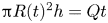 ${\rm \pi} R(t)^{2} h=Qt$), we have $R(t)\propto (Q/h)^{1/2}t^{1/2}$, where $Q$ and $h$ remain constant in the data plotted. Hence, the linear scaling of $R_{in}(t)$ and $R(t)$ with $t^{1/2}$ confirm that the size of the particle accumulation zone must also grow proportionately with $R(t)$, which is consistent with self-similarity in $\bar \phi$.
3. Theory
3.1. Theoretical formulation: suspension balance model
In order to rationalise the self-similar behaviour of the  $\bar {\phi }$ profile, we hereby treat the particle–oil mixture as a continuum and develop a thin-film suspension model of our system. We consider the injection of a suspension inside a Hele-Shaw cell from the centre $O$ and define a $z$–
$z$– $r$ cylindrical coordinate system as illustrated in the schematics of figure 2(c). The present model is based on the suspension balance model by Nott & Brady (Reference Nott and Brady1994), which includes a two-phase formulation expressed for the bulk suspension and particulate phase.
The mass and momentum conservation equations for the mixture are given as
 \begin{gather} \boldsymbol{\nabla} \boldsymbol{\cdot} \boldsymbol{u}=0, \end{gather}
 \begin{gather}\boldsymbol{\nabla} \boldsymbol{\cdot}{\boldsymbol{\mathsf{T}}}=0, \end{gather}
where  $\boldsymbol {u}$ is the velocity of the suspension and ${\boldsymbol{\mathsf{T}}}$ is the total stress tensor. Similarly, the governing equations for the particle phase correspond to
 \begin{gather} \dfrac{\partial \phi}{\partial t}+ \boldsymbol{\nabla} \boldsymbol{\cdot} (\phi{\boldsymbol{u}}^{p} )=0, \end{gather}
 \begin{gather}\boldsymbol{\nabla} \boldsymbol{\cdot} {\boldsymbol{\mathsf{T}}}^{p}+\boldsymbol{F}=0, \end{gather}
where the superscript ‘ $p$’ refers to the particle phase; hence, $\boldsymbol {u}^{p}$ and ${\boldsymbol{\mathsf{T}}}^{p}$ represent the particle velocity and stress tensor, respectively.
The inter-phase drag force depends on the relative velocity between the particle and the bulk suspension:
 \begin{equation} \boldsymbol{F}={-}18 \frac{\mu_l}{d^{2}} \frac{\phi}{H(\phi)}(\boldsymbol{u}^{p} - \boldsymbol{u} ),\end{equation}
where the hindrance function corresponds to  $H(\phi )=(1-\phi )^{5}$ (Richardson & Zaki Reference Richardson and Zaki1954); $\mu _l$ is the viscosity of the suspending liquid. By combining with (3.1a), we can rewrite (3.2a) as
 \begin{equation} \frac{\partial \phi}{\partial t}+{\boldsymbol{u}} \boldsymbol{\cdot} \boldsymbol{\nabla} \phi={-}\boldsymbol{\nabla}\boldsymbol{\cdot} [\phi ({\boldsymbol{u}}^{p} -{\boldsymbol{u}}) ]. \end{equation}
The bulk suspension and particle phase are coupled through the constitutive equations for stress tensors
 \begin{gather} {\boldsymbol{\mathsf{T}}}={-}p {\boldsymbol{\mathsf{I}}}+{\boldsymbol{\mathsf{T}}}^{p}+2 \mu_l{{\boldsymbol{\mathsf{E}}}}, \end{gather}
 \begin{gather}{\boldsymbol{\mathsf{T}}}^{p}={\boldsymbol{\mathsf{T}}}_n^{p}+2(\mu_s(\phi)-\mu_l) {{\boldsymbol{\mathsf{E}}}}, \end{gather}
where  ${\boldsymbol{\mathsf{I}}}$ is the identity matrix, and ${\boldsymbol{\mathsf{E}}}$ is the bulk suspension rate of strain tensor. We take the following form of the normal stress of the particulate phase in each direction as
 \begin{equation} {\boldsymbol{\mathsf{T}}}_n^{p}={-}\mu_n(\phi) \dot{\gamma}\left( \begin{array}{@{}ccc@{}} 1 & 0 & 0 \\ 0 & \lambda_2 & 0 \\ 0 & 0 & \lambda_3 \end{array} \right)\quad \begin{array}{l} (\textrm{flow}) \\ (\textrm{velocity gradient}) \\ (\textrm{vorticity}) \end{array}, \end{equation}
where  $\lambda _2$ and $\lambda _3$ are scalar parameters first defined by Bird, Armstrong & Hassager (Reference Bird, Armstrong and Hassager1987) independent of $\phi$, which can be determined from rheological measurements of the suspension (Morris & Brady Reference Morris and Brady1998; Zarraga, Hill & Leighton Reference Zarraga, Hill and Leighton2000; Boyer, Guazzelli & Pouliquen Reference Boyer, Guazzelli and Pouliquen2011). Note that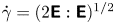 $\dot {\gamma }=(2{\boldsymbol{\mathsf{E}}} : {\boldsymbol{\mathsf{E}}})^{1/2}$ is the strain rate; $\mu _s(\phi )$ and $\mu _n(\phi )$ are the effective shear and normal viscosities of the bulk suspension, respectively.
Amongst different empirical models for the effective viscosities (Krieger Reference Krieger1972; Morris & Boulay Reference Morris and Boulay1999; Zarraga et al. Reference Zarraga, Hill and Leighton2000), we presently employ those developed by Morris & Boulay (Reference Morris and Boulay1999), written as
 \begin{gather} \dfrac{\mu_s(\phi)}{\mu_l}=1+2.5\phi\left(1-\dfrac{\phi}{ \phi_m} \right)^{{-}1}+0.1 \left(\dfrac{\phi}{\phi_m} \right)^{2} \left(1-\dfrac{\phi}{\phi_m} \right)^{{-}2}, \end{gather}
 \begin{gather}\dfrac{\mu_n(\phi)}{\mu_l}=0.75 \left(\dfrac{\phi}{\phi_m} \right)^{2}\left(1-\dfrac{\phi}{\phi_m} \right)^{{-}2}, \end{gather}
where  $\phi _m=0.6$ is the maximum packing fraction of particles.
Our experiments are performed by injecting the mixture at a constant volumetric flow rate  $Q$. Hence, the incompressibility of the mixture requires the following constraint for local volume conservation:
 \begin{equation} Q=2 {\rm \pi}r \int_{{-}h/2}^{h/2} u_r \, \textrm{d} z,\end{equation}
where the subscript ‘ $r$’ corresponds to the radial component of the velocity field and $h$ is the channel gap thickness. In addition, the condition of no particle flux at the walls corresponds to
 \begin{equation} \phi u^{p}_z\vert_{z={\pm} h/2}=\left[\frac{d^{2}H(\phi)}{18\mu_l} [ \boldsymbol{\nabla} \boldsymbol{\cdot} {\boldsymbol{\mathsf{T}}}^{p} ]_z+\phi u_z\right]_{z={\pm} h/2}=0,\end{equation}
where the subscript ‘ $z$’ is the vertical component.
We hereby introduce dimensionless variables (denoted with an asterisk) to simplify the governing equations:
 \begin{equation} \left.\begin{array}{c@{}} \displaystyle r^{*}=\dfrac{r}{R_0}, \quad z^{*}=\dfrac{z}{\epsilon R_0},\quad \mu_{s/n}^{*}=\dfrac{\mu_{s/n}}{\mu_l}, \quad p^{*}=\dfrac{p}{\mu_{l}U_0R_0/h^{2}},\\ \displaystyle u_r^{*}=\dfrac{u_r}{U_0},\quad u_z^{*}=\dfrac{u_z}{\epsilon U_0}, \quad {\boldsymbol{\mathsf{T}}}^{p*}=\dfrac{{\boldsymbol{\mathsf{T}}}^{p}}{\mu_l U_0/h}, \quad t^{*}=\dfrac{t}{R_0/U_0}, \end{array}\right\} \end{equation}
where  $R_0$ is the characteristic radial distance and $\epsilon \equiv h/R_0$, while the characteristic radial velocity is defined as $U_0\equiv Q/({\rm \pi} R_0h)$. In particular, since $R(t)=(Q/({\rm \pi} h))^{1/2}t^{1/2}$, the time-dependent location of the interface can be expressed as $R^{\ast }=t^{\ast 1/2}$ based on the dimensionless variables defined.
3.2. Model assumptions and multiple-time-scale expansion
Our model rests on a few assumptions based on the experimental set-up and our observations. First, we reasonably assume  $\epsilon =h/R_0\ll 1$, as $R_0\sim O(10^{-1})\ \textrm {m}$ and $h\sim O(10^{-3})\ \textrm {m}$ based on our experiments. Next, we consider two important time scales that characterise the current system: $\tau _z$, the time scale of particle migration across the thin gap and $\tau _r$, the time scale of particle advection in the $r$-direction. While $\tau _r\sim R_0/U_0$, $\tau _z$ can be derived as $\tau _z \sim (h^{2}/d^{2})\dot \gamma ^{-1}$, where $\dot \gamma \sim U_0/h$, by examining (3.4) and (3.3). Alternatively, $\tau _z=h^{2}/D$, where $D$ is the shear-induced diffusivity that scales as $d^{2}\dot \gamma$ (Leshansky, Morris & Brady Reference Leshansky, Morris and Brady2008; Griffiths & Stone Reference Griffiths and Stone2012). Then, the ratio of the time scales corresponds to $\tau _z/\tau _r = \epsilon \chi$, where $\chi = (h/d)^{2}\gg 1$.
Based on the characteristic experimental parameters, the typical value of  $\epsilon \chi$ ranges from $0.6$ to $1$. Nonetheless, we consider the limit where $\epsilon \chi$ is a small parameter, such that $\epsilon \ll \epsilon \chi \ll 1$, for the following reasons. First, assuming $\epsilon \chi \ll 1$ allows us to simplify our present analysis and to systematically add the effects of Taylor dispersion into our transport equation, in the manner of Ramachandran (Reference Ramachandran2013). Second, the disparity of the time scales is evident in the experimental plot of $\bar \phi$ (see figure 2b), in which the size of Region I – the transient region near the injection centre – is consistently small compared to the overall radial distance. This implies that the time it takes for particles to migrate across the thin gap must be small compared to that of particle transport in the radial direction. Hence, it is reasonable to assume $\tau _z\ll \tau _r$, or $\epsilon \ll \epsilon \chi \ll 1$, as a starting point in the present analysis. Finally, we neglect the transient region near the injection centre (Region I) and only focus on Regions II and III in our model.
Given the assumptions above, we first employ the lubrication approximations and reduce the governing equations based on  $\epsilon \ll 1$. Second, we follow the multiple-time-scale expansion by Ramachandran (Reference Ramachandran2013) and break up the time variable into the short (i.e. $t^{*}_1 = t^{*}$) and long (i.e. $t^{*}_2 = \epsilon \chi t^{*}$) time scales, such that
 \begin{equation} \frac{\partial}{\partial t^{*}} = \frac{\partial}{\partial t_1^{*}} + (\epsilon\chi)\frac{\partial}{\partial t_2^{*}} + O((\epsilon\chi)^{2}).\end{equation}
Then, the dependent variables can be expanded in the order of  $\epsilon \chi$. We denote the leading order term with the superscript ‘ $(0)$’ and the term linear in $\epsilon \chi$ with ‘ $(1)$’ (e.g. $\phi = \phi ^{(0)}+(\epsilon \chi )\phi ^{(1)} + O((\epsilon \chi )^{2})$). Note that all dependent and independent variables henceforth are presented in their dimensionless form unless otherwise noted; the asterisk $(\ast )$ is subsequently dropped for brevity.
Specifically, we model our current system in two steps. First, we compute the particle concentration profiles (e.g.  $\phi ^{(0)}$, $\phi ^{(1)}$) and radial velocity profiles (e.g. $u_r^{(0)}$, $u_r^{(1)}$) in the order by order fashion. This yields the expression for the particle flux with respect to the local depth-averaged particle concentration, up to $O(\epsilon \chi )$. Second, we utilise the expression for the particle flux and derive an evolution equation for $\bar \phi$ based on the particle volume conservation, which is solved numerically with appropriate initial and boundary conditions. Overall, our model procedure closely follows the derivation of Ramachandran (Reference Ramachandran2013), which we frequently refer to for more details.
3.3. Leading order solutions
Combining (3.1b) and (3.5a), the momentum conservation equations of the bulk suspension can be obtained to the leading order in  $\epsilon$ and in $\epsilon \chi$ as
 \begin{gather} \partial_r p^{(0)}=\frac{\partial}{\partial z}[\mu_s(\phi^{(0)})\partial_z u^{(0)}_r], \end{gather}
 \begin{gather}\partial_z p^{(0)}=0. \end{gather}
Note that we have assumed the flow to be axisymmetric; hence, the equation in the  $\theta$-direction is neglected. Also, at the leading order, the particle transport equation (3.4), combined with (3.2b), (3.3), (3.5b) and (3.6), yields
 \begin{equation} \frac{\partial}{\partial z}\left[ H(\phi^{(0)}) \frac{\partial}{\partial z} \left(\lambda_2 \mu_n(\phi^{(0)}) \frac{\partial u^{(0)}_r}{\partial z} \right) \right]=0, \end{equation}
while the no-flux boundary condition (3.9) reduces to
 \begin{equation} \left.\frac{\partial}{\partial z} \left(\lambda_2 \mu_n(\phi^{(0)}) \frac{\partial u^{(0)}_r}{\partial z} \right) \right\rvert_{z={\pm} h/2}=0.\end{equation}
By integrating (3.13) subject to (3.14), we obtain
 \begin{equation} \mu_n (\phi^{(0)}) \partial_z u^{(0)}_r=\textrm{const.} \end{equation}
Similarly, based on (3.12b) and the condition  $\partial _z u_r (z=0)=0$, we can integrate (3.12a) with respect to $z$ to obtain
 \begin{equation} \mu_s (\phi^{(0)})\partial_z u^{(0)}_r=\partial_r p^{(0)} z. \end{equation}
 Next, by combining (3.16) and (3.15), we can obtain an implicit expression for  $\phi ^{(0)}(z)$ as
 \begin{equation}
\frac{1}{g(\phi^{(0)}(z))} = \frac{\partial_{r} p^{(0)} z}{\rm const.} = C_{0} z.
\end{equation}
\begin{equation}
\frac{1}{g(\phi^{(0)}(z))} = \frac{\partial_{r} p^{(0)} z}{\rm const.} = C_{0} z.
\end{equation}
where  $g(\phi ^{(0)})\equiv \mu _n (\phi ^{(0)})/\mu _s (\phi ^{(0)})$ and $C_0$ is a constant independent of $z$ but may have a dependence on $r$. Then, we integrate (3.16) again and apply no-slip boundary conditions (i.e. $u^{(0)}_r(z= \pm 1/2)=0$) to obtain an expression for the mixture velocity,
 \begin{equation} u^{(0)}_r(z)=\int_{{-}1/2}^{z} \frac{\partial_r p^{(0)} \tilde{z}}{\mu_{s}(\phi^{(0)}(\tilde{z}))} \, \textrm{d} \tilde{z}, \end{equation}
where
 \begin{equation} \partial_r p^{(0)}=\left[2r\int_{{-}1/2}^{1/2} \int_{{-}1/2}^{z} \frac{\tilde{z}}{\mu_{s}(\phi^{(0)}(\tilde{z}))} \, \textrm{d} \tilde{z}\, \textrm{d} z\right]^{{-}1} \end{equation}
can be determined from the volume conservation of the suspension as
 \begin{equation} 1=2r\int_{{-}1/2}^{1/2} u^{(0)}_r\, \textrm{d} z. \end{equation}
 Finally, we compute the resultant local particle concentration profile  $\phi ^{(0)}(z)$ from (3.17), by treating the depth-averaged particle concentration, $\bar {\phi }=\int _{-1/2}^{1/2} \phi ^{(0)} \, \textrm {d} z$, as a known parameter. By systematically varying the value of $\bar \phi$, we obtain a complete set of solutions for $u^{(0)}_r(z)$ and $\phi ^{(0)}(z)$, examples of which are plotted in figure 4. The plot of $\phi ^{(0)}(z)$ in figure 4(a) shows that there is a higher concentration at the centreline, $z=0$, owing to the shear-induced migration of particles. Then, the corresponding velocity profiles, $u^{(0)}_r$, are normalised by the local mean velocity, $\bar {u} = \int _{-1/2}^{1/2} u^{(0)}_{r}\, \textrm {d} z$, and plotted for varying $\bar \phi$. As shown in figure 4(b), the velocity profile becomes more blunt at $z=0$ for increasing $\bar \phi$. This is consistent with the physical picture of particle aggregation near the centreline. With $u^{(0)}_r(z)$ and $\phi ^{(0)}(z)$ thus known, we subsequently compute the dimensionless particle flux, $f^{(0)}$, as a function of $\bar \phi$:
 \begin{equation} f^{(0)}=2r\int_{{-}1/2}^{1/2} u^{(0)}_r (z)\phi^{(0)}(z) \, \textrm{d} z. \end{equation}
(a) Local particle concentration profile  $\phi ^{(0)}$ and (b) the normalised velocity profile, $u_r^{(0)}/\bar {u}$, as a function of $z$ for varying depth-averaged concentrations $\bar \phi$.

3.4.  $O(\epsilon \chi )$ solutions

Within the lubrication framework, we consider the governing equations at  $O(\epsilon \chi )$ to derive $u^{(1)}_r$ and $\phi ^{(1)}$. At $O(\epsilon \chi )$, the momentum conservation of the mixture leads to
 \begin{gather} \partial_r p^{(1)}=\frac{\partial}{\partial z}[\mu_s\partial_z u_r]^{(1)}, \end{gather}
 \begin{gather}\partial_z p^{(1)}=0, \end{gather}
while (3.4) reduces to
 \begin{equation} \frac{\partial \phi^{(0)}}{\partial t_1}+ u_r^{(0)} \frac{\partial \phi^{(0)}}{\partial r} +u_z^{(0)} \frac{\partial \phi^{(0)}}{\partial z} = \frac{1}{18}\frac{\partial}{\partial z}\left[ H(\phi^{(0)}) \frac{\partial}{\partial z} \left( \lambda_2 \mu_n \left| \frac{\partial u_r}{\partial z} \right| \right)^{(1)} \right]. \end{equation}
 We then integrate (3.23) from  $z=-1/2$ to $z=1/2$. With no particle flux condition at the walls (i.e. (3.9) at $O(\epsilon \chi )$), the right-hand side of (3.23) vanishes upon integration, such that
 \begin{equation} \int_{{-}1/2}^{1/2} \frac{\partial \phi^{(0)}}{\partial t_1} \, \textrm{d} z +\int_{{-}1/2}^{1/2}\left[u_r^{(0)} \frac{\partial \phi^{(0)}}{\partial r} +u_z^{(0)} \frac{\partial \phi^{(0)}}{\partial z}\right]\, \textrm{d} z=0 . \end{equation}
On the left-hand side, we apply the chain rule and integration by parts to the second and third terms, respectively, so that
 \begin{gather} \int_{{-}1/2}^{1/2} u^{(0)}_r {\partial_r}{\phi^{(0)}} \, \textrm{d} z=\dfrac{1}{r} \partial_{r} \left(r \int_{{-}1/2}^{1/2}u^{(0)}_r\phi^{(0)} \, \textrm{d} z \right)-\int_{{-}1/2}^{1/2} \frac{1}{r}\partial_r(r u^{(0)}_r) \phi^{(0)} \, \textrm{d} z, \end{gather}
 \begin{gather}\int_{{-}1/2}^{1/2}u^{(0)}_z {\partial_{z}}{\phi^{(0)}} \, \textrm{d} z=(\phi^{(0)} u^{(0)}_z)|_{z=1/2}-(\phi^{(0)} u^{(0)}_z)|_{z={-}1/2}- \int_{{-}1/2}^{1/2} \phi^{(0)} \partial_z u^{(0)}_z \, \textrm{d} z. \end{gather}
Based on the impermeability boundary condition and continuity, we derive the following particle transport equation at  $O(\epsilon \chi )$:
 \begin{equation} \frac{\partial\bar\phi}{\partial t_1} + \frac{1}{2r}\frac{\partial f^{(0)}}{\partial r} = 0.\end{equation}
 By combining (3.23) with (3.26) and employing chain rules (e.g.  $\partial _r = \partial _r\bar {\phi }\partial _{\bar \phi }$), we re-write the left-hand side of (3.23) as
 \begin{equation} -\frac{\partial \phi^{(0)}}{\partial \bar{\phi}}\frac{\textrm{d} f^{(0)}}{\textrm{d} \bar{\phi}}\frac{1}{2r}\frac{\partial \bar{\phi}}{\partial r} +u_r^{(0)} \frac{\partial \phi^{(0)}}{\partial \bar{\phi}}\frac{\partial \bar{\phi}}{\partial r} +u_z^{(0)} \frac{\partial \phi^{(0)}}{\partial z}, \end{equation}
where  $u^{(0)}_z=r^{-1}{\partial r}\int ^{1/2}_{z}ru_r^{(0)}\, \textrm {d} \tilde {z}$ based on continuity. After some algebraic manipulation, (3.23) becomes
 \begin{equation} S_2(\bar{\phi},z)\frac{1}{r}\frac{\partial \bar{\phi}}{\partial r}=\frac{1}{18}\frac{\partial}{\partial z}\left[ H(\phi^{(0)}) \frac{\partial}{\partial z} \left( \lambda_2\mu_n(\phi) \left| \frac{\partial u_r}{\partial z} \right| \right)^{(1)} \right], \end{equation}
where
 \begin{equation} S_2(\bar{\phi}, z)= \frac{\partial \phi^{(0)}}{\partial \bar{\phi}}\left[ru^{(0)}_r - \frac{1}{2}\frac{\partial f^{(0)}}{\partial r}\right] + \frac{\partial \phi^{(0)}}{\partial z}\frac{\partial}{\partial \bar{\phi}}\int^{1/2}_z ru^{(0)}_r(\bar{\phi},\tilde{z}) \, \textrm{d} \tilde{z}.\end{equation}
Finally, integrating (3.28) and applying appropriate boundary conditions leads to
 \begin{equation} \phi^{(1)}=S_7({\bar{\phi},z}) \frac{\partial \bar{\phi}}{\partial r},\end{equation}
where  $S_7$ is a function of $z$ for given $\bar {\phi }$. In addition, combining (3.30) with the momentum equations (3.22a) and (3.22b) yields the expression for the perturbation velocity, $u_r^{(1)}$:
 \begin{equation} u_r^{(1)}=S_{11}({\bar{\phi},z})\frac{1}{r} \frac{\partial \bar{\phi}}{\partial r}.\end{equation}
The detailed derivations of  $\phi ^{(1)}$ and $u_r^{(1)}$, as well as the expressions of $S_7$ and $S_{11}$, are included in the appendix.
Notably,  $\phi ^{(1)}$ and $u_r^{(1)}$ depend on the gradient of $\bar \phi$ in the radial direction and on $\bar \phi$, as distinct from the leading order terms. To probe the physical meaning of $\phi ^{(1)}$ and $u_r^{(1)}$ more closely, we plot the functions, $S_7$ and $S_{11}$, in figure 5. The plot of $S_7$ in figure 5(a) shows that $\phi ^{(1)}$ is positive near the walls ( $z=1/2$) and negative near the centreline before sharply vanishing at $z=0$; these effects are increasingly less pronounced at higher $\bar \phi$. This suggests that when $\bar \phi$ increases with $r$ (i.e. $\partial _r\bar \phi > 0$), the effects of shear-induced migration may become mitigated, as the particle concentration is reduced near the centreline and increases near the walls. Similarly, as shown in the plot of $S_{11}$ in figure 5(b), $u_r^{(1)}$ is positive near $z=0$ and becomes negative for increasing $z$ before reaching zero at the walls. While this trend is consistent for all $\bar \phi$, it is reduced at larger $\bar \phi$. This implies that for $\partial _r\bar \phi > 0$, the velocity profile becomes less blunt near the centreline, where the corresponding particle concentration decreases.
Here, (a)  $S_7$ and (b) $S_{11}$ plotted as a function of $z$ for varying depth-averaged concentrations $\bar {\phi }$.

This dependence of  $\phi ^{(1)}$ and $u_r^{(1)}$ on $\partial _r\bar \phi$ will directly impact the dynamics of particle accumulation through the corresponding perturbation in the particle flux, or $f^{(1)}$. With $\phi ^{(0)}$, $u_r^{(0)}$, $\phi ^{(1)}$ and $u_r^{(1)}$ known, we compute $f^{(1)}$ as
 \begin{equation} f^{(1)}=2r\int_{{-}1/2}^{1/2}[u^{(0)}_r (z)\phi^{(1)}(z) + u^{(1)}_r (z)\phi^{(0)}(z)]\, \textrm{d} z = 2S_{12}(\bar{\phi}) \frac{\partial \bar{\phi}}{\partial r},\end{equation}
where
 \begin{equation} S_{12}(\bar{\phi}) = \int_{{-}1/2}^{1/2} [S_7(\bar{\phi}, z)ru^{(0)}_r (z) + S_{11}(\bar{\phi}, z)\phi^{(0)}(z)]\, \textrm{d} z.\end{equation}
As shown in figure 6(b),  $S_{12}(\bar {\phi })$ is negative and its magnitude generally decreases with $\bar {\phi }$, while $f^{(0)}$ monotonically increases with $\bar \phi$. Hence, the particle flux must increase more slowly owing to this perturbation in the flux, as particles accumulate on the interface, or as $\partial _r\bar \phi > 0$. We conjecture that this mitigation in the particle flux may lead to the gradual accumulation of particles, which will be fully examined in the next section.
(a) The numerical solution of the leading order flux,  $f^{(0)}$, is plotted as a function of depth-averaged concentration $\bar {\phi }$. The solid line indicates the linear fit. (b) The solution of $S_{12}$ is plotted for varying depth-averaged concentration, $\bar {\phi }$, and is fitted with a function $-0.0022\times \phi ^{-1.399}$.

4. Particle transport equation and self-similarity
In order to compute  $\bar \phi$, we must consider the depth-averaged particle transport equation that combines terms up to $O((\epsilon \chi )^{2})$. Hence, we start by integrating (3.4) over the thin gap at $O((\epsilon \chi )^{2})$. By utilising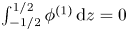 $\int _{-1/2}^{1/2} \phi ^{(1)}\, \textrm {d} z = 0$ and taking the same steps as $O(\epsilon \chi )$ (e.g. (3.25a) and (3.25b)), we obtain
 \begin{equation} \frac{\partial\bar\phi}{\partial t_2} + \frac{1}{2r}\frac{\partial f^{(1)}}{\partial r} = 0.\end{equation}
Finally, we combine (3.26) and (4.1) to derive the following depth-averaged particle transport equation:
 \begin{equation} \frac{\partial \bar{\phi}}{\partial t} + \frac{1}{2r}\frac{\partial f^{(0)}}{\partial r}+(\epsilon\chi)\frac{1}{r}\frac{\partial}{\partial r}\left [S_{12}(\bar{\phi}) \frac{\partial \bar{\phi}}{\partial r} \right]=0.\end{equation}
To find the similarity solution to (4.2), we seek a solution with the following structure:
 \begin{equation} \bar \phi = \frac{1}{t^{\alpha}} \psi\left(\frac{r}{\sqrt{t}}\right) : = \frac{1}{t^{\alpha}} \psi(\xi),\end{equation}
where  $\alpha$ and $\psi$ can be found. Substituting it into (4.2), we have
 \begin{align} -\alpha \xi \psi(\xi) - \frac{1}{2} \psi'(\xi) \xi^{2} + \frac{1}{2}{f^{(0)}}'(\bar\phi)\psi'(\xi) + \frac{1}{t^{\alpha + {1}/{2}}} S_{12}'(\bar\phi) \psi'(\xi)^{2} + \frac{1}{\sqrt{t}} S_{12}(\bar \phi) \psi''(\xi) \!=\! 0. \end{align}
 Note from the plot of  $f^{(0)}$ in figure 6(a), we may reasonably approximate $f^{(0)}$ as a linear function in $\bar \phi$, so that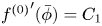 ${f^{(0)}}'(\bar \phi ) = C_1$ for a constant $C_1$. If we assume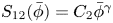 $S_{12} (\bar \phi ) = C_2 \bar \phi ^{\gamma }$ for some constant $C_2$ and $\gamma$, and choose $\alpha$ such that $\alpha \gamma +\frac {1}{2}=0$, then (4.4) reduces to
 \begin{equation} -\alpha \xi \psi(\xi) - \tfrac{1}{2} \psi'(\xi) \xi^{2} + C_1\psi'(\xi) + \gamma (\psi^{\gamma-1} \psi'(\xi)^{2} + \psi^{\gamma} \psi''(\xi)) =0, \end{equation}
which provides a rule to determine  $\psi$. As a result, $\bar \phi =t^{1/(2\gamma )}\psi (r/\sqrt {t})$ is a self-similar solution to (4.2). In figure 6(b), we fit $S_{12}(\bar \phi )$ with $-0.0022\times \bar \phi ^{-1.399}$ and show that the latter approximates the former with a slight deviation. This deviation explains why our solution is not exactly self-similar. However, as shown in figure 6(b), the deviation is so small that particles are expected to accumulate in an approximately self-similar manner. Hence, this approximate self-similar nature of (4.1) is consistent with the experimental measurements of $\bar \phi$ in figure 2(b).
4.1. Simulation results: comparison with experiments
We solve (4.2) numerically using the upwind finite difference scheme, by applying the following initial and boundary conditions:
 \begin{gather} \bar{\phi}(r>0,t=0)=0, \end{gather}
 \begin{gather}\bar{\phi}(r=0,t)=\bar{\phi}_{up}(\phi_0), \end{gather}
 \begin{gather}\bar{\phi}(r>R(t),t)= 0. \end{gather}
The initial condition (4.6a) indicates that there are no particles inside the domain at  $t=0$, while (4.6c) imposes zero particle concentration downstream of the immiscible interface, $R(t)$. The latter simultaneously satisfies the condition of zero particle flux for $r>R(t)$. In addition, we impose $\bar {\phi }$ at the inlet to be $\bar {\phi }_{up}$, the constant depth-averaged particle concentration in Region II. In the experiments, the depth-averaged concentration is $\phi _0$ at the inlet and gradually transitions to $\bar {\phi }_{up}$ downstream (Region I). As the current model considers only Regions II and III, it is reasonable to use $\bar {\phi }(r=0)=\bar {\phi }_{up}$ as our boundary condition, such that the flux at the inlet is equal to the upstream particle flux $f(\bar {\phi }_{up}) = f^{(0)}(\bar {\phi }_{up}) + (\epsilon \chi )f^{(1)}(\bar {\phi }_{up})$.
Hence, we first calculate  $\bar {\phi }_{up}$ by revisiting the solution of $\phi ^{(0)}(z)$ in § 3.3. Specifically, we compute $\phi ^{(0)}(z)$ from (3.17), subject to the particle volume conservation in the fully developed limit (Region II): $\phi _0=2r\int _{-1/2}^{1/2} u^{(0)}_r\phi ^{(0)} \, \textrm {d} z$. Note that the solutions in this regime reduce to the steady-state results of a one-dimensional channel flows, as $\partial _r\bar \phi = 0$ ensures that $\phi ^{(1)}=0$. Finally, we obtain $\bar \phi _{up}$ by integrating the resultant $\phi ^{(0)}(z)$ across the thin gap. Figure 7 shows the plot of $\phi _0-\bar \phi _{up}$ versus $\phi _0$ from theory (solid line), together with the experimental measurements (symbols). The results show a qualitative match between theory and experiments, although the theoretical prediction of $\phi _0-\bar \phi _{up}$ is persistently larger than the experimental measurements. We subsequently utilise $\bar {\phi }_{up}(\phi _0)$ from our model as the boundary condition in (4.6b).
The difference between the initial concentration and the depth-averaged particle concentration,  $\phi _0-\bar {\phi }_{up}$, in Region II is plotted as a function of $\phi _0$. The solid line represents the numerical solution from the simplified suspension balance model with the constraint of the particle volume conservation. The square markers indicate the experimental data for $h=1.4 \ \textrm {mm}$.

We examine some characteristic solutions to (4.2) for varying values of  $\epsilon \chi$. Note that the second term in (4.2) characterises the radial advection of particles, while the last term corresponds to the radial diffusion, or Taylor dispersion, of particles that acts to smooth out the changes in $\bar \phi$ in the $r$-direction. Hence, the value of $\epsilon \chi$ determines the relative importance of Taylor dispersion versus particle advection in the particle transport equation. Figure 8 shows the plot of $\bar \phi (r)$ at $t=14 \,{\rm s}$ for $\phi _0=0.2$ with values of $\epsilon \chi$ ranging from 0.4 to 1. As expected, the increase in $\bar \phi$ becomes less steep, as the value of $\epsilon \chi$ is systematically increased. Following this increase, $\bar \phi$ is shown to rapidly decrease to zero at the interface, largely independent of the value of $\epsilon \chi$.
The numerical solution of depth-averaged particle concentration,  $\bar {\phi }_{up}$, as function of $r$ is plotted for various values of $\epsilon \chi$ at $t=14\,{\rm s}$ and $\phi _0=0.2$. As $\epsilon \chi$ increases, the increase in $\bar {\phi }_{up}$ becomes less steep.

Next, we compare the numerical solutions to (4.2) with our experiments for  $\phi _0=0.2$ and $0.25$, respectively, which fall in the regime of clear particle accumulation and no viscous fingering. Here we empirically set the values of $\epsilon \chi$ to best fit the experimental results of $\bar {\phi }$, as shown in figure 9(a) and (b). The fitted value corresponds to $\epsilon \chi =0.9$ at both concentrations. While the actual values of $\epsilon \chi$ used do not strictly meet the assumption of $\epsilon \chi \ll 1$, we note that the characteristic size of Taylor diffusion in (4.2) is still an order of magnitude smaller than that of the advection term, as $|S_{12}|\sim O(0.01)$ and $f^{(0)}\sim O(0.1)$ in figure 6. The numerical solutions of $\bar {\phi }$ are plotted as a function of dimensional $r$ (in solid lines) at six different times, $t$. The markers indicate the experimental measurements of the depth-averaged particle concentrations.
Comparison of the numerical solutions of  $\bar \phi$ to the experiments for (a) $\phi _0=0.2$ and (b) $\phi _0=0.25$, both with $\epsilon \chi =0.9$. Solid lines in the plots indicate the theoretical results, while the solid symbols are experimental measurements. The inset plots indicate the theoretical results of $\bar {\phi }$ versus $r/R$ in Region III. The solutions of the dimensional flux, $f$, are also compared with the experimental measurements for (c) $\phi _0=0.2$ and (d) $\phi _0=0.25$, respectively. Note that $r$ is a dimensional radial coordinate.

The numerical solutions agree well with the experimental observation for both concentrations except for the over-prediction of  $\bar {\phi }$ near the interface particularly for $\phi _0=0.25$. This over-prediction is expected given that our current model sets $\bar \phi (r=0)=\bar \phi _{up}$ and neglects Region I in which $\bar \phi$ gradually decreases from $\phi _0$ at $r=0$ to $\bar \phi _{up}$ downstream. We have also plotted the numerical solutions of $\bar {\phi }$ as a function of $r/R$ in Region III in the inset of figure 9(a). It clearly shows that our theoretical results are also self-similar, despite small deviations near the interface, which is consistent with the experimental observations in figure 2(b). In addition, the numerical solutions of the dimensional flux, $f$, are plotted and compared with the experimental results in figure 9(c,d) for both concentrations at varying $t$. The theoretical results are in qualitative agreement with the experiments at all times.
Overall, our reduced model has demonstrated the shear-induced migration of the particles far upstream and the presence of the fluid–fluid interface are barebones physical ingredients that can lead to particle accretion on the interface in the current geometry. Then, the gradual accumulation of particles is achieved through the inclusion of the perturbation in the particle flux that depends on both local  $\bar \phi$ and the gradient of $\bar \phi$ in the radial direction. This perturbation appears in the particle transport equation as the axial diffusion term, which mitigates how steeply $\bar \phi$ increases towards the interface. The resultant particle transport equation yields solutions that are approximately self-similar and in remarkable agreement with the experimental data.
5. Summary and conclusions
In summary, our work has focused on understanding the self-similar behaviour of particle accumulation observed in suspension flow, through experiments and theoretical modelling. This particle accumulation at the advancing interface is attributed to the shear-induced migration of particles far up stream, which causes the particles to assume a faster average velocity than the mixture. We first carry out the experiments by injecting the suspension into the Hele-Shaw cell with varying initial particle concentrations,  $\phi _0$, at a constant volume flow rate $Q$. We extract the depth-averaged particle volume fraction $\bar {\phi }$ and the particle flux $f(r)$ via image processing. The evolution of $\bar {\phi }$ as a function of $r$ collapses on to a single curve when $r$ is normalised by the instantaneous position of the interface, $R(t)$. We divide the collapsed curves of $\bar {\phi }(r/R(t))$ into three distinct regions: Regions I, II and III. In particular, Region II refers to the region where the suspension reaches a quasi-fully developed flow with constant $\bar {\phi } = \bar {\phi }_{up}$, while $\bar {\phi }$ increases towards the interface in Region III. We experimentally quantify the boundary between Region II and Region III as $R_{in}(t)$. The linear scaling of both $R_{in}(t)$ and $R(t)$ with respect to $t^{1/2}$ also confirms the self-similar growth of particle accumulation.
We develop a thin-film model to rationalise the self-similarity of  $\bar {\phi }$ based on the suspension balance model. By combining the lubrication approximations and multiple-time-scale expansion, we obtain the depth-averaged upstream concentration, $\bar {\phi }_{up}$, as well as the particle flux (i.e. $f^{(0)}$ and $f^{(1)}$) for given local $\bar {\phi }(r)$ and the gradient of $\bar {\phi }(r)$. Then, we derive a depth-averaged particle transport equation by considering the conservation of the particle volume. In particular, the perturbation in the flux appears in the particle transport equation as the axial diffusion term that mitigates how steeply $\bar \phi$ increases towards the interface. The resultant particle transport equation yields solutions that are approximately self-similar, and in remarkable agreement with the experimental data.
The good match between theory and experiments demonstrates that our reduced model successfully captures the self-similar behaviour of particle accumulation on the advancing fluid–fluid interface. However, the model has a number of limitations that need to be addressed. For instance, the validity of the model for  $\epsilon \chi \sim O(1)$ is questionable, despite the good agreement with the experiments. In addition, the present model results suggest that the presence of the fountain flow and the shape of the meniscus play a minimal role in the dynamics of particle accretion, which is not well understood. Finally, resolving the particle dynamics near the fluid–fluid interface is only the first step in predicting the threshold particle concentration necessary to trigger particle-induced viscous fingering. In particular, previous experimental measurements have shown that $\bar {\phi }$ needs to attain a critical slope with respect to $r$ before miscible fingering is observed (Luo et al. Reference Luo, Chen and Lee2018). However, the physical and mathematical basis for this observation is currently not well understood. Hence, predicting the onset of fingering requires building on the current model for $\bar {\phi }(r,t)$ to derive a fully nonlinear two-dimensional model of the suspension flow inside a thin gap.
Acknowledgements
We acknowledge Dr F. Xu for providing the experimental data featured in this manuscript.
Funding
This work is partially supported by the National Science Foundation: DMR 2003706 for R.L. and S.L.; DMS 1846854 for L.W.
Declaration of interests
The authors report no conflict of interest.
Appendix A. Derivations of $\phi ^{(1)}$ and $u^{(1)}_r$


Let us first define the following terms:
 \begin{equation} S_1(\bar{\phi},z)=\int_{z}^{1/2}-\frac{\tilde{z}}{\mu_s(\phi)}\, \textrm{d} \tilde{z},\quad M(\bar{\phi})=\int^{1/2}_{{-}1/2}S_1(\bar{\phi},z)\, \textrm{d} z \end{equation}
so that we can rewrite  $\partial _rp^{(0)}$ and $u_r^{(0)}$ as
 \begin{gather} \partial_rp^{(0)} = \frac{1}{2rM(\bar{\phi})}, \end{gather}
 \begin{gather}u_r^{(0)}(\bar{\phi}, r, z)=\frac{S_1(\bar{\phi},z)}{2r M(\bar{\phi})}. \end{gather}
 We integrate equation (3.28) from  $z$ to $1/2$ using the no-particle flux condition (3.9) to obtain
 \begin{equation} \frac{18}{\lambda_2 H({\phi^{(0)}})} \left[ \int^{1/2}_{z} -S_2(\tilde{z}, \bar{\phi})\, \textrm{d} \tilde{z} \frac{1}{r}\frac{\partial \bar{\phi}}{\partial r} \right ]=\frac{\partial}{\partial z} \left(g(\phi) \mu_s(\phi) \left| \frac{\partial u_r}{\partial z} \right| \right)^{(1)}. \end{equation}
After another integration from  $0$ to $z$, (A3) becomes
 \begin{equation} \frac{18}{\lambda_2} \left[ -\int^{z}_{0} \frac{\displaystyle \int^{1/2}_{\tilde z} -S_2(\tilde{z}', \bar{\phi})\, \textrm{d} \tilde{z}'}{H(\phi^{(0)})} \, \textrm{d} {\tilde z} \frac{1}{r}\frac{\partial \bar{\phi}}{\partial r}+B_0(r,t) \right] =\left(g(\phi) \mu_s(\phi) \frac{\partial u_r}{\partial z} \right)^{(1)},\end{equation}
where  $B_0(r,t)$ is a constant to be determined later.
We now expand the right-hand side of (A4), so that
 \begin{equation} \left(g(\phi) \mu_s(\phi) \frac{\partial u_r}{\partial z} \right)^{(1)}=g(\phi^{0})\left(\mu_s(\phi) \frac{\partial u_r}{\partial z} \right)^{(1)}+\frac{\textrm{d} g (\phi^{(0)})}{\textrm{d} \phi^{(0)}}\phi^{(1)}\left(\mu_s(\phi) \frac{\partial u_r}{\partial z} \right)^{(0)}. \end{equation}
 Combining (A5) with (A4), we obtain an expression for  $\phi ^{(1)}$ as
 \begin{align} \phi^{(1)}&=\frac{1}{\displaystyle \frac{\textrm{d} g(\phi^{(0)})}{\textrm{d} \phi^{(0)}} \left(\mu_s(\phi) \frac{\partial u_r}{\partial z}\right)^{(0)} } \left\{\vphantom{\left.\quad -g(\phi^{(0)})\left( \mu_s(\phi) \frac{\partial u_r}{\partial z} \right)^{(1)} \right\}} \frac{18}{\lambda_2} \left[ S_3(z, \bar{\phi})\frac{1}{r}\frac{\partial \bar{\phi}}{\partial r} +B_0(r,t) \right]\right.\nonumber\\ &\left.\quad -g(\phi^{(0)})\left( \mu_s(\phi) \frac{\partial u_r}{\partial z} \right)^{(1)} \right\},\end{align}
where
 \begin{equation} S_3(z, \bar{\phi})=\int^{z}_{0} \frac{\displaystyle \int^{1/2}_{\tilde{z}} S_2(\tilde{z}', \bar{\phi})\, \textrm{d} \tilde{z}'}{H(\phi^{(0)})} \, \textrm{d} {\tilde z}. \end{equation}
From (3.12a) and the definition of (A2a), we have
 \begin{equation} \left(\mu_s(\phi)\frac{\partial u_r}{\partial z} \right)^{(0)}=\frac{z}{2rM}, \end{equation}
while the momentum equations (3.22a) and (3.22b) yield
 \begin{equation} \left(\mu_s (\phi) \frac{\partial u_r}{\partial z} \right)^{(1)}= \frac{\partial p^{(1)}}{\partial r}z,\end{equation}
where  $\partial _rp^{(1)}$ is independent of $z$. Therefore, the second term on the right-hand side of (A6) can be written as
 \begin{equation} g(\phi^{(0)})\left(\mu_s(\phi) \frac{\partial u_r}{\partial z} \right)^{(1)}=g(\phi^{(0)})\frac{\partial p^{(1)}}{\partial r}z. \end{equation}
 Since  $g(\phi ^{(0)})z$ is also independent of $z$ according to (3.17), the second term on the right-hand side of (A6), $[-g(\phi ^{(0)}) (\mu _s(\phi )\partial _z u_r)^{(1)}]$, must be a function of $r$ and $t$ only, which will be combined with $B_0(r,t)$ as a single constant $B(r,t)$. Then, (A6) can be finally simplified as
 \begin{equation} \phi^{(1)}=\frac{1}{\displaystyle \frac{\textrm{d} g(\phi^{(0)})}{\textrm{d} \phi^{(0)}} \frac{z}{2rM(\bar{\phi})}} \left\{ \frac{18}{\lambda_2} \left[ S_3(z, \bar{\phi})\frac{1}{r}\frac{\partial \bar{\phi}}{\partial r} +B(r,t)\right]\right\}. \end{equation}
The constant  $B(r,t)$ can be determined using the constraint $\int ^{1/2}_{-1/2}\phi ^{(1)}\, \textrm {d} z=0$, such that
 \begin{equation} B(r,t)={-}\frac{S_5({\bar{\phi}})}{S_6({\bar{\phi}})}\frac{1}{r}\frac{\partial \bar{\phi}}{\partial r}. \end{equation}
Note that
 \begin{gather} S_4({\bar{\phi},z})=\frac{\textrm{d} g(\phi^{(0)})}{\textrm{d} \phi^{(0)}} \frac{z}{2M(\bar{\phi})}, \end{gather}
 \begin{gather}S_5({\bar{\phi}})=\int_{{-}1/2}^{1/2}\frac{S_3({\bar{\phi},z})}{S_4({\bar{\phi},z})}\, \textrm{d} z, \end{gather}
 \begin{gather}S_6({\bar{\phi}})=\int_{{-}1/2}^{1/2}\frac{1}{S_4({\bar{\phi},z})}\, \textrm{d} z. \end{gather}
Therefore, (A11) can be further expressed as
 \begin{equation} \phi^{(1)}=\frac{1}{S_4({\bar{\phi},z})}\left\{\frac{18}{\lambda_2} \left[ S_3(\bar{\phi},z) -\frac{S_5(\bar{\phi})}{S_6(\bar{\phi})} \right] \right\}\frac{\partial \bar{\phi}}{\partial r}.\end{equation}
Finally, we simplify (A14) as
 \begin{equation} \phi^{(1)}=S_7({\bar{\phi},z}) \frac{\partial \bar{\phi}}{\partial r},\end{equation}
by defining
 \begin{equation} S_7({\bar{\phi},z})=\frac{1}{S_4({\bar{\phi},z})}\left\{ \frac{18}{\lambda_2} \left[ S_3({\bar{\phi},z})- \frac{S_5({\bar{\phi}})}{S_6({\bar{\phi}})} \right] \right\}. \end{equation}
 To compute the velocity profile at  $O(\epsilon \chi )$, we expand the left-hand side of (A9) as
 \begin{equation} \left(\mu_s \frac{\partial u_r}{\partial z} \right)^{(1)}=\mu_s(\phi^{(0)})\frac{\partial u_r^{(1)}}{\partial z}+ \frac{\textrm{d} \mu_s(\phi^{(0)})}{\textrm{d} \phi^{(0)}}\phi^{(1)}\frac{\partial u_r^{(0)}}{\partial z}. \end{equation}
Substituting equation (A17) into (A9) and rearranging, we obtain
 \begin{equation} \frac{\partial u_r^{(1)}}{\partial z}=\frac{z}{\mu_s(\phi^{(0)})}\frac{\partial p^{(1)}}{\partial r}-\frac{1}{\mu_s(\phi^{(0)})}\frac{\textrm{d} \mu_s(\phi^{(0)})}{\textrm{d} \phi^{(0)}}\phi^{(1)}\frac{\partial u_r^{(0)}}{\partial z}. \end{equation}
Now, we integrate (A18) from  $z$ to $1/2$ and apply the no-slip boundary condition, which yields
 \begin{equation} u_r^{(1)}= S_1(\bar{\phi},z)\frac{\partial p^{(1)}}{\partial r}-\int^{1/2}_{z}-\frac{1}{\mu_s(\phi^{(0)})}\frac{\textrm{d} \mu_s(\phi^{(0)})}{\textrm{d} \phi^{(0)}}\phi^{(1)}\frac{\partial u_r^{(0)}}{\partial z} \, \textrm{d} \tilde{z},\end{equation}
subject to
 \begin{equation} r\int^{1/2}_{{-}1/2}u_r^{(1)}\, \textrm{d} z=0. \end{equation}
 Using the previous constraint and the expression of  $\phi ^{(1)}$, we can write the expression of $\partial _r p^{(1)}$ as
 \begin{equation} \frac{\partial p^{(1)}}{\partial r}=\frac{\displaystyle \int_{{-}1/2}^{1/2}\int_{z}^{1/2}-\frac{1}{\mu_s(\phi^{(0)})}\frac{\textrm{d} \mu_s(\phi^{(0)})}{\textrm{d} \phi^{(0)}}\frac{\partial u_r^{(0)}}{\partial z}S_7(\bar{\phi},\tilde{z})\, \textrm{d} \tilde{z}\, \textrm{d} z}{M(\bar{\phi})} \frac{\partial \bar{\phi}}{\partial r}.\end{equation}
Again, from (3.12a) and the definition of (A2a), we have
 \begin{equation} \frac{\partial u_r^{(0)}}{\partial z} =\frac{1}{\mu_s(\phi^{(0)})}\frac{z}{2rM}. \end{equation}
Then,  $u_r^{(1)}$ can be expressed as
 \begin{equation} u_r^{(1)}=[ S_{10}(\bar{\phi},z)-S_8(\bar{\phi},z) ] \frac{1}{r}\frac{\partial \bar{\phi}}{\partial r} \end{equation}
from (A21), by defining
 \begin{gather} S_8({\bar{\phi},z})=\int_{z}^{1/2}-\frac{1}{\mu_s^{2}(\phi^{(0)})}\frac{\textrm{d} \mu_s(\phi^{(0)})}{\textrm{d} \phi^{(0)}}\frac{\tilde{z}}{2M(\bar{\phi})}S_7(\bar{\phi},\tilde{z})\, \textrm{d} \tilde{z}, \end{gather}
 \begin{gather}S_9({\bar{\phi}})=\frac{\displaystyle \int_{{-}1/2}^{1/2}S_8({\bar{\phi},z})}{M(\bar{\phi})} \, \textrm{d} z, \end{gather}
 \begin{gather}S_{10}({\bar{\phi},z})=S_1(\bar{\phi},z)S_{9}(\bar{\phi}). \end{gather}
We finally simplify (A23) as
 \begin{equation} u_r^{(1)}=S_{11}({\bar{\phi},z})\frac{1}{r} \frac{\partial \bar{\phi}}{\partial r}, \end{equation}
where
 \begin{equation} S_{11}({\bar{\phi},z})=S_{10}(\bar{\phi},z)-S_8(\bar{\phi},z). \end{equation}


 Open access

