





Policy Significance Statement
The research in this paper presents a data-driven policy framework for deploying dynamic electronic road pricing systems that address urban congestion and air pollution. By using AI-based optimization to adjust tolls hourly, the model enables governments to implement adaptive, demand-responsive pricing strategies grounded in real-time environmental and traffic data. The inclusion of multiple stakeholder objectives—government revenue, commuter cost, and environmental health—ensures that resulting policies are balanced, equitable, and politically viable. Applied to London, the model shows that meaningful improvements in air quality and congestion can be achieved with only marginal price increases, demonstrating cost-effectiveness and public acceptability. These findings provide actionable guidance for cities seeking scalable transport policies that align short-term behavioural incentives with long-term sustainability goals. The research supports a shift from static regulation to dynamic policymaking, where pricing tools can be used proactively to manage demand, respond to pollution surges, and advance net-zero urban mobility agendas.
1. Introduction
Over the past few decades, rapid socio-economic development and increased vehicle ownership have led to an increase in traffic congestion and air pollution in the City of London. Though the days of “Moderate” or higher pollution have been relatively well controlled in the past years (DEFRA, 2024), it is worth pointing out that the UK Air Quality Standard (AQS) Objectives, which are legally defined thresholds established under the Environment Act 1995 and informed by EU directives, may fall short of the World Health Organization (WHO) air quality guidelines. In the case of PM10, the WHO objectives are only half of the UK AQS Objectives (WHO, 2005). The United Kingdom (UK) has been the first country in the world to announce in 2011 that conventional car and van sales will end by 2040 to encourage the adoption of zero emission vehicle, the government still recognizes the urgency to explore other options to enable immediate reduction of roadside NO2 concentration (The Joint Air Quality Unit of the Government of the UK, 2017).
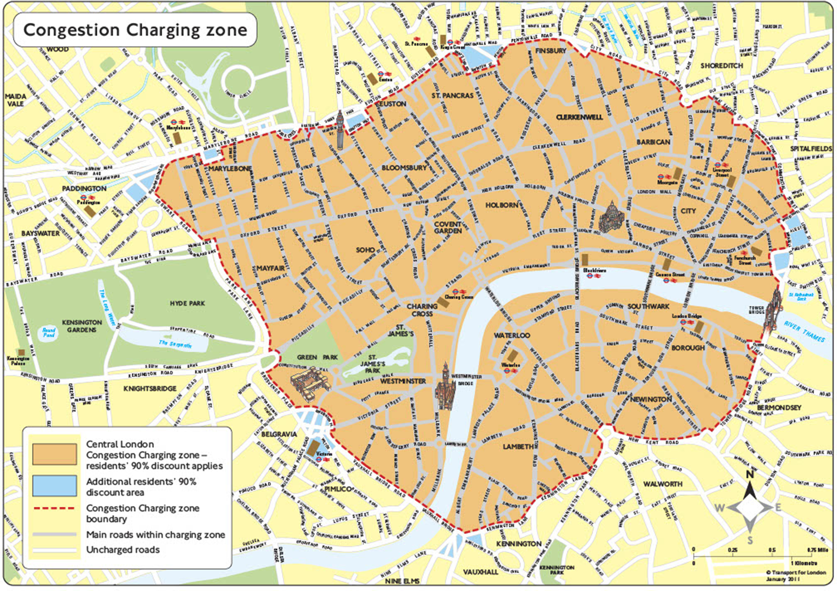
To reduce the air pollutants from vehicles, a few static electronic road pricing (ERP) models have been implemented by the London government. The Congestion Charge Scheme (CCS) was introduced first and covers the Congestion Charge Zone (CCZ). The details of the CCZ in operation during the time frame used in this paper (2008–2019) are shown in Figure 1 (Transport for London, n.d.). During this period, the CCS operates from 0700 to 1800, inclusive, and only during weekdays. The Toxicity-Charge (T-Charge) and its successor, the Ultra Low Emission Zone (ULEZ), were introduced soon after, operating in the CCZ as well. However, despite some tangible impacts, the three are all static models, and thus are not fully optimized to minimize traffic congestion and air pollution levels. For improved performance, the transition to dynamic models would be more desirable from an efficiency perspective.
The London Congestion Charge Zone (CCZ) from 2008 to 2019.
The overall objective of this paper is to minimize traffic congestion and air pollution levels in the City of London through a dynamic ERP model. The deliverables are (1) an optimized dynamic ERP model for the CCZ that improves the optimization efficiency of the static one, and (2) a one-day pricing schedule for the entire CCZ, based on the air pollution and traffic congestion values of the previous days, within the operational hours of the CCZ. The dynamic ERP model for the ULEZ is not included in this paper due to the lack of data. However, with sufficient time and data accumulation, the dynamic model developed for the CCZ can be readily extended to the ULEZ. Due to the data irregularities caused by the COVID-19 pandemic, data from 2020 to 2022 are excluded from this study; however, data from 2023 onwards have been used. The problem is formulated as a multi-stakeholder, multi-objective optimization problem (MS-MOP), involving three key stakeholders—the government, vehicle owners, and environmental organizations—and three primary objectives: reducing air pollution, alleviating traffic congestion, and optimizing pricing. To solve this problem, three evolutionary algorithms are employed and compared: Non-dominated Sorting Genetic Algorithm II (NSGA-II), NSGA-III, and Unified NSGA-III (U-NSGA-III).
Once human behaviour changes due to the implementation of the dynamic ERP, the algorithm can be trained with the new data gathered after the behaviour change to create new price schedules to maintain the equilibrium between the changes in traffic congestion and the derivation of the price.
2. Related work
Related works have shown significant progress in the use of dynamic road pricing to reduce both congestion and pollution in urban environments. Many foundational studies analysed the impact of road pricing on either traffic congestion or air pollution (Atkinson et al., Reference Atkinson, Barratt, Armstrong, Anderson, Beevers, Mudway, Green, Derwent, Wilkinson and Tonne2009; Beevers et al., Reference Beevers, Carslaw, Dajnak, Stewart, Williams, Kelly and Kelly2016). Early dynamic pricing models used dynamic programming, neural networks (Teodorović and Edara, Reference Teodorović and Edara2007), discrete non-linear mathematical programming (Chang and Hsueh, Reference Chang and Hsueh2006), or city-wide zone pricing (Soylemezgiller et al., Reference Soylemezgiller, Kuscu and Kilinc2013). Other papers estimate the impacts of dynamic systems on vehicle owner behaviour (Brent and Gross, Reference Brent and Gross2018) or on network performance (Joksimovic et al., Reference Joksimovic, Bliemer, Bovy and Verwater-Lukszo2005). In particular, Chen et al. (Reference Chen, An, Sharon, Hanna, Stone, Miao and Soh2018) look at creating a dynamic electronic toll collection system by formulating the problem as a Markov Decision Process (MDP). While it showed great results in traffic alleviation by outperforming existing static and dynamic tolling schemes, it only focuses on small-scale traffic networks. Besides looking at dynamic systems, Hanna et al. (Reference Hanna, Sharon, Boyles and Stone2019) look at the effects of selecting only compliant agents for an opt-in tolling system. This opt-in tolling method was found to have a considerable increase in social welfare with just a small percentage of compliant agents. However, these papers look at a toll spatial format, rather than a zone spatial format. Furthermore, they only consider the price and maximizing the total vehicles that reach their destination (Chen et al., Reference Chen, An, Sharon, Hanna, Stone, Miao and Soh2018) or price and total travel time (Hanna et al., Reference Hanna, Sharon, Boyles and Stone2019). Schubert et al. (Reference Schubert, Sys, Vanelslander and Roumboutsos2022) focused on congestion management via No-Queue Road Pricing (NQRP), setting real-time tolls to maintain target speeds. Our work differs by using trained schedules instead of real-time pricing, allowing for behaviour adaptation and changes in pollution patterns.
Recent literature has emphasized the potential of artificial intelligence in dynamic pricing systems. Lu et al. (Reference Lu, Hong and Wang2024) propose MAGT-toll, a multi-agent reinforcement learning (RL) model using transformers to dynamically set tolls. Their simulations demonstrate substantial reductions in congestion and travel time across varying demand levels. Similarly, Parishad et al. (Reference Parishad, Yildirimoglu and Hickman2025) developed a deep RL double-DQN model for cordon pricing in multi-modal networks. Even with input demand errors, their approach maintained close-to-optimal flow and outperformed feedback-control policies. Prior studies report that learning-based dynamic tolling can reduce peak congestion by 18–25% and CO2 emissions by 12% in EV corridors. These studies suggest that RL-based tolling can adapt flexibly to dynamic urban conditions and yield significant environmental and efficiency gains.
Other algorithmic approaches have also been explored. Wang et al. (Reference Wang, Jin and Yin2021) developed a control-theoretic model for high-occupancy toll (HOT) lanes, adjusting tolls based on real-time queue lengths while estimating drivers’ value of time. They show convergence to an optimal state of usage with minimal queues, offering stability in pricing and flow control.
From a game-theoretic and optimization standpoint, dynamic pricing has been modelled as a bilevel optimization problem. Chiu et al. (Reference Chiu, Wang and Liu2023) demonstrate that marginal-cost toll updates on an arc-based model converge to socially optimal equilibria. Tan et al. (Reference Tan, Sun, Zhu, Qin, Zhao and Wang2024) design a bilevel model that prioritizes minimizing human exposure to emissions, revealing trade-offs between emissions and travel time. Zong et al. (Reference Zong, Zeng and Li2024) evaluate different toll structures and find that combining distance- and time-based pricing reduces CO2 emissions by 23% and shifts 5% of drivers towards sustainable modes.
Recent surveys (e.g., Sharon et al., Reference Sharon, Levin, Hanna, Rambha, Boyles and Stone2017) note that self-interested routing leads to suboptimal equilibria, and that dynamic, segment-level tolling can better align user behaviour with system-wide efficiency.
Empirical studies support the effectiveness of dynamic pricing. Egbo and Marinov (Reference Egbo and Marinov2023) analyse multiple cities, including London, and find that only those with congestion pricing schemes (e.g., London, Stockholm) are on track to meet WHO air quality goals. NO2 levels in these cities have seen 20–30% reductions. While London’s scheme remains fixed-time, its expansion and the introduction of Ultra Low Emission Zones (ULEZ) reflect its continued evolution. Cities like Milan and Jakarta provide comparative lessons, and the literature suggests that incorporating real-time responsiveness and multi-objective metrics into pricing can significantly amplify benefits. Another study (Saharan et al., Reference Saharan, Bawa and Kumar2020) explores the pros and cons of a dynamic scheme and the recent dynamic pricing techniques and details the potential of different methods used for dynamic models. In particular, it analyses evolutionary optimization-based techniques for dynamic congestion pricing, which is a topic associated with our current study.
Recent literature also underscores the importance of sustainable urban transport in achieving long-term climate and social goals, and that aligning local transport planning with global sustainability objectives can significantly reduce congestion and greenhouse gas emissions. Ribeiro et al. (Reference Ribeiro, Dias and Mendes2024) demonstrate that meeting CO2 reduction targets necessitates large-scale modal shifts to active and public modes—over 60% of trips must be walking, or cycling, and another 30% must be transit to meet their 2040 carbon neutrality targets.
The intersection of policy and equity is also explored in the literature. Verity et al. (Reference Verity, Poirier Stephens, Lin, Ottoni, Bourgeois, Kestens, Fuller, Manaugh and Winters2025) study sustainable transportation projects in Canadian cities and find a tendency to prioritize active travel and safety, while other benefits such as air quality and health equity are underemphasized. Munkácsy et al. (Reference Munkácsy, Földes, Miskolczi and Jászberényi2024) examine EU Sustainable Urban Mobility Plans (SUMPs) and show that while sustainability themes are central, many plans rely on incremental changes and lack transformative measures aligned with the UN SDGs. This signals a gap between high-level commitments and actionable, equity-oriented policies.
Lukic Vujadinovic et al. (Reference Lukic Vujadinovic, Damnjanovic, Cakic, Petkovic, Prelevic, Pantovic, Stojanovic, Vidojevic, Vranjes and Bodolo2024) apply RL to optimize bus schedules in Serbia, showing that real-time, adaptive systems can boost service reliability and satisfaction while cutting environmental impacts. These advances point towards a growing role for AI in sustainable mobility systems.
A key empirical study by Gökasar and Bakioglu (Reference Gökasar and Bakioglu2018) investigates the effect of real-time traffic information on travel behaviour using a multinomial logit model at Istanbul Technical University. They find that travellers receiving live updates are more likely to switch to less congested routes, and that this behaviour varies by socioeconomic status and tech adoption. Their findings support the inclusion of behavioural responsiveness in pricing models—such as ERP—and strengthen the foundation for adaptive, dynamic pricing based on real-time feedback.
Our approach diverges from prior work by modelling a Multi-Stakeholder Multi-Objective Problem (MS-MOP), incorporating both traffic congestion and air pollution through a zone-based spatial format tailored to the UK context. Unlike works that focus solely on congestion (e.g., Chen et al., Reference Chen, An, Sharon, Hanna, Stone, Miao and Soh2018; Hanna et al., Reference Hanna, Sharon, Boyles and Stone2019) or use single-objective tolling, our model allows for stakeholder parameterization to reflect long-term preferences. While Schubert et al.’s real-time tolling leaves little room for behaviour adaptation, our trained price schedule captures shifts in driver response over time. An exploratory analysis (Garzon et al., Reference Garzon, Reppenhagen and Müller2022) is closely related to our paper and simulates a road pricing scheme dictated by air pollution within the city of Berlin. It investigates the implications of a highly dynamic road pricing schedule based on temporally evolving low-emission zones (LEZ) whose shape, size, and location are determined by the air quality levels. This aspect is very similar to the concept of sub-regions used in our paper, where each sub-region is a set of smaller regions of the CCZ and has its own dynamic price schedule based on air pollution and traffic congestion levels in that sub-region. While it varies from the idea that the shape and size of the LEZ is defined by the air pollution, having a spatially fine-grained distribution replicates the effect that can be achieved by small enough sub-regions. The paper showcases the potential of such a model with a simulation showing only minor detours to reach the destination. Moreover, it mentions that the dynamic pricing scheme based on air pollution was considered in isolation as part of a more complex pricing scheme, which our paper addresses by looking at both air pollution and traffic congestion, as well as approaching it from a multi-stakeholder aspect.
Lastly, while some studies explore stakeholder negotiation using game theory (e.g., Yildirim and Hearn, Reference Yildirim and Hearn2005; Wang et al., Reference Wang, Ehrgott, Dirks and Gupta2014), ours contributes by combining evolutionary optimization (inspired by NSGA-II) with stakeholder-defined weights to simulate realistic policy trade-offs. The multi-stakeholder aspect is crucial to the paper, as can be seen in Vosough et al.’s work (Vosough et al., Reference Vosough, de and Lindsey2022). It uses a dynamic traffic network simulator to showcase the welfare gains and benefits of cordon tolls, a toll for a restricted region of the city centre, with regard to emissions and road congestion. It is mentioned that most cities in developed countries have larger congestion externalities, while cities in developing countries have higher levels of air pollution. This problem is addressed by the multi-stakeholder aspect, which allows the stakeholders to set parameters through discussion to give either the air pollution factors or traffic congestion factors attention, allowing for long-term goals in the reduction of emissions and congestion to be met, and creating a more flexible model.
Therefore, we introduce a zone-based dynamic ERP model that integrates multi-stakeholder preferences and balances both congestion and air pollution objectives. Unlike prior dynamic tolling studies, which often optimize a single goal (e.g., traffic flow or emissions) or assume static pricing, our model simultaneously optimizes across multiple stakeholder-defined objectives using a multi-objective evolutionary algorithm. While evolutionary algorithms (e.g., NSGA-II) have been applied in traffic management, existing applications do not incorporate stakeholder differentiation or address the practical challenges of long-term deployment in real-world contexts like London’s CCZ while optimizing for multiple objectives, such as both air pollution and congestion objectives. Our approach goes further by embedding stakeholder preferences as tunable parameters, enabling policy flexibility and retraining in response to behavioural shifts or evolving urban priorities. Key contributions include:
-
• The introduction of the first dynamic ERP model to employ a multi-objective evolutionary algorithm with a view towards deployment, to address real-life traffic congestion and air pollution challenges in the City of London. Based on this, real-life and context-specific air pollution and traffic congestion reduction measures can be proposed, with the model and policy suggestions being easily extended to other metropolitan hubs.
-
• A novel parameterization of stakeholder externalities via adjustable weights, enabling the model to adapt to evolving policy goals through retraining. The weight allows focus on particular objectives as decided by policy goals, even after retraining the algorithm after a change in human behaviour, and hence can help reach a long-term goal throughout multiple trainings of the algorithm. This provides an effective method for incorporating the multi-stakeholder aspect of the problem.
-
• The provision of the first dynamic ERP model to provide stakeholders with the ability to meet both short- and long-term goals, through the application of a multi-objective evolutionary algorithm and unique problem formulation, as well as the extension of the composite method of modelling stakeholder preferences to other related studies which require multi-stakeholder negotiation/agreement. Here, short-term goals refer to the time period that any one of the various optimum price schedules is used for. Switching to a different price schedule will result in immediate, short-term changes.
-
• The novel development of a fully automatic dynamic ERP model, which allows ERP decisions to be performed automatically and continuously.
3. Methodology
This study proceeded through the following steps. First, a set of core assumptions was defined to operationalize the dynamic ERP system within a Central Congestion Zone (CCZ). Second, the problem was formally structured as a Multi-Stakeholder Multi-Objective Problem (MS-MOP), including the definition of inputs (air quality and traffic congestion factors), stakeholder parameter weights, and multiple objective functions. Third, a set of mathematical constraints linking ERP pricing to pollution and congestion metrics was derived from historical data (2008–2016) using regression methods. Fourth, air quality and traffic flow data were collected from official UK government sources and spatially mapped using Voronoi-based sub-regions based on air quality monitoring stations. Fifth, extensive data pre-processing was conducted, including interpolation and imputation, and the derivation of missing PM $ {}_{2.5} $
values from PM
$ {}_{2.5} $
values from PM $ {}_{10} $
where needed. Sixth, stakeholder weights were assigned using a data-driven approach based on deviation from AQS, and all variables were scaled to ensure comparability. Seventh, multiple NSGA evolutionary algorithms were applied to generate candidate ERP price schedules. Finally, the Pareto-optimal schedules were evaluated across air quality, traffic congestion, and pricing objectives, and NSGA-II was selected due to its capacity to generate a diverse set of high-quality solutions.
$ {}_{10} $
where needed. Sixth, stakeholder weights were assigned using a data-driven approach based on deviation from AQS, and all variables were scaled to ensure comparability. Seventh, multiple NSGA evolutionary algorithms were applied to generate candidate ERP price schedules. Finally, the Pareto-optimal schedules were evaluated across air quality, traffic congestion, and pricing objectives, and NSGA-II was selected due to its capacity to generate a diverse set of high-quality solutions.
3.1. Assumptions
The following assumptions have been made for this study:
-
1. All charges are deducted from the vehicle owners automatically.
-
2. Navigation software that enables optimized route calculation and price level communication at any given time exists and is widely used by the population at large. This assumption, along with Assumption 1, means that the vehicle owners will have to pay the lowest possible charges and do not need to worry about paying manually. In case the vehicle owners would like to plan their trip timings, the software also allows them to check the price levels.
-
3. The changes in human behaviour exhibited inside the CCZ due to the dynamic ERP will not change by sub-region. Here, a sub-region is defined as a section of a zone. This section can ideally be defined as a regular polygon in shape, assuming the inputs to the model are spatially fine-grained enough with respect to the regions within the zone. This assumption can be justified if the sub-regions are relatively small.
-
4. The charge is incurred at the entrance to a sub-region, and if multiple sub-regions are entered, then the price charged to the vehicle owner switches to the highest price. In case the deduction has already occurred, any extra amount incurred will be charged. This assumption will prevent multiple overlapping charges and will charge the vehicle owner with the highest charge incurred.
3.2. Problem formulation
The problem formulation here is generalized to allow for better understanding and provide extensions for future work. The problem formulation consists of five steps, namely, input definition, modelling stakeholder externalities, objective function, output definition, and optimization constraints.
3.2.1. Input definition
The inputs to the problem can be generalized as follows:
-
• Air Quality Factor (AQF) $ j={\alpha}_j;j=1,\dots, J $
;
$ J $
is the number of AQFs.
$ j={\alpha}_j;j=1,\dots, J $
;
$ J $
is the number of AQFs. -
• Traffic Congestion Factor (TCF)
$ k={\beta}_k;k=1,\dots, K $
;
$ K $
is the number of TCFs.




To obtain the desired spatiotemporal resolution, the CCZ can be subdivided into $ N $
different sub-regions, with each sub-region being denoted by
$ N $
different sub-regions, with each sub-region being denoted by $ i $
. Similarly, the time in consideration can be subdivided into
$ i $
. Similarly, the time in consideration can be subdivided into $ T $
segments, with each segment being denoted by
$ T $
segments, with each segment being denoted by $ t $
. After this, the inputs by sub-region
$ t $
. After this, the inputs by sub-region $ i $
and time
$ i $
and time $ t $
can be written as follows:
$ t $
can be written as follows:
-
• AQF
$ j={\alpha}_{j,i,t};j\in \left[1,J\right];i\in \left[0,N-1\right];t\in \left[1,T\right] $
-
• TCF
$ k={\beta}_{k,i,t};k\in \left[1,K\right];i\in \left[0,N-1\right];t\in \left[1,T\right] $


3.2.2. Modelling stakeholder externalities
To model long-term stakeholder externalities, a novel stakeholder-parameters (SHPs) approach is utilized. SHP here refers to the weight given to each goal. This approach involves determining certain SHPs initially through a multi-stakeholder negotiation. The SHPs can be determined either through discussion or by using existing data. For example, if a particular AQF is violating its required standard more than the other AQFs in consideration, then it can be given a larger weight to denote its increased necessity of reduction based on how great its violation is. The SHPs can then be determined by the stakeholders involved, such as the government, which can set a greater weight to the factors it feels need to be addressed urgently. These SHPs are denoted as follows:
-
• Weight of AQF
$ j={\lambda}_{j,i} $
, which gives the weight for AQF
$ j $
in the sub-region
$ i $
-
• Weight of TCF
$ k={\sigma}_{k,i} $
, which gives the weight for TCF
$ k $
in the sub-region
$ i $
-
• Weight of sub-region
$ i={l}_i $


It is also important that the sum of each category of SHPs should equate to one, so that they function as designed. For example, air pollution would need the sum of the weights given to all AQFs to be equal to 1. Thus, the following constraints unique to the SHPs must be observed:
 $$ {\left[\sum \limits_{i=1}^J{\lambda}_{j,i}=1\right]}_{i=0}^{N-1},\hskip3em {\left[\sum \limits_{k=1}^K{\sigma}_{k,i}=1\right]}_{i=0}^{N-1},\hskip3em \sum \limits_{i=0}^{N-1}{l}_i=1. $$
To justify the use of stakeholder weights (SHPs), it is important to note that these parameters exist to direct attention to factors that require more urgent intervention. Stakeholders, such as government agencies, environmental agencies, and road users, can have different priorities based on health, regulatory, or operational concerns. For example, stakeholders may decide that reducing PM $ {}_{2.5} $
is more urgent than reducing NO
$ {}_{2.5} $
is more urgent than reducing NO $ {}_2 $
, especially if PM
$ {}_2 $
, especially if PM $ {}_{2.5} $
levels are consistently above regulatory limits while NO
$ {}_{2.5} $
levels are consistently above regulatory limits while NO $ {}_2 $
levels are relatively closer to compliance. In this study, the SHPs for the air quality factors were not arbitrarily set, but instead derived using a data-driven approach: we calculated how far the average values of NO2 and PM
$ {}_2 $
levels are relatively closer to compliance. In this study, the SHPs for the air quality factors were not arbitrarily set, but instead derived using a data-driven approach: we calculated how far the average values of NO2 and PM $ {}_{2.5} $
in each sub-region deviated from their respective UK AQS. The greater the deviation from the AQS, the higher the assigned weight for that factor. These deviation-based scores were then normalized so that the total weight across all AQFs summed to 1. This ensures that those pollutants that are further from regulatory compliance receive proportionally greater emphasis during the optimization process. This method maintains transparency, reflects empirical air quality needs, and offers flexibility for stakeholders to revisit and adjust weights in response to evolving environmental or policy priorities.
$ {}_{2.5} $
in each sub-region deviated from their respective UK AQS. The greater the deviation from the AQS, the higher the assigned weight for that factor. These deviation-based scores were then normalized so that the total weight across all AQFs summed to 1. This ensures that those pollutants that are further from regulatory compliance receive proportionally greater emphasis during the optimization process. This method maintains transparency, reflects empirical air quality needs, and offers flexibility for stakeholders to revisit and adjust weights in response to evolving environmental or policy priorities.
3.2.3. Objective functions
There are three objective functions in this problem, corresponding to air quality, traffic congestion, and price. These can be constructed using the inputs and SHPs defined in the previous two subsections. For sub-region $ i $
and time
$ i $
and time $ t $
, the objective functions can be written as shown below:
$ t $
, the objective functions can be written as shown below:
 $$ {\phi}_{i,t}^{AQ}=\sum \limits_{j=1}^J{\lambda}_{j,i}{\alpha}_{j,i,t},\hskip1.7em {\phi}_{i,t}^{TC}=\sum \limits_{k=1}^K{\sigma}_{k,i}{\beta}_{k,i,t},\hskip1.7em {\phi}_{i,t}^P={y}_{i,t}. $$
For all $ N $
sub-regions, taking into consideration that all SHPs are employed, the objective functions can then be rewritten as follows:
$ N $
sub-regions, taking into consideration that all SHPs are employed, the objective functions can then be rewritten as follows:
 $$ {\displaystyle \begin{array}{c}{\Phi}_t^{AQ}=\sum \limits_{i=0}^{N-1}{l}_i{\phi}_{i,t}^{AQ}=\sum \limits_{i=0}^{N-1}\sum \limits_{j=1}^J{l}_i{\lambda}_{j,i}{\alpha}_{j,i,t}\\ {}{\Phi}_t^{TC}=\sum \limits_{i=0}^{N-1}{l}_i{\phi}_{i,t}^{TC}=\sum \limits_{i=0}^{N-1}\sum \limits_{k=1}^K{l}_i{\sigma}_{k,i}{\beta}_{k,i,t}\\ {}{\Phi}_t^P=\sum \limits_{i=0}^{N-1}{l}_i{\phi}_{i,t}^P=\sum \limits_{i=0}^{N-1}{l}_i{y}_{i,t}.\end{array}} $$
Taking a mean over all temporal segments allows the objective functions to be written as below:
 $$ {\Phi}^{AQ}=\frac{1}{T}\sum \limits_{t=1}^T{\Phi}_t^{AQ},\hskip1.7em {\Phi}^{TC}=\frac{1}{T}\sum \limits_{t=1}^T{\Phi}_t^{TC},\hskip1.7em {\Phi}^P=\frac{1}{T}\sum \limits_{t=1}^T{\Phi}_t^P. $$
3.2.4. Output definition
The optimization of multiple objective functions through a multi-objective evolutionary algorithm leads to OC an optimum output candidate, where each candidate is a price schedule. These candidates form points which lie on a multi-dimensional Pareto-optimal surface, or Pareto front, and are all optimal, differentiated by trade-offs in the objectives. To fulfil short-term goals, stakeholders can choose the price schedule that most suits their needs at that point in time.
Thus, this problem has one direct output—a list of OC candidates, with each candidate containing a schedule of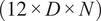 $ \left(12\times D\times N\right) $
prices, where D denotes the number of days and N denotes the number of sub-regions. Each value in a candidate is the price at a certain time for a certain sub-region.
$ \left(12\times D\times N\right) $
prices, where D denotes the number of days and N denotes the number of sub-regions. Each value in a candidate is the price at a certain time for a certain sub-region. $ 12 $
is used as the CCS is only operational for 12 hours a day. However, this problem also has
$ 12 $
is used as the CCS is only operational for 12 hours a day. However, this problem also has $ \left(J+K\right) $
indirect outputs for each output candidate, which correspond to J air quality lists, and K traffic congestion lists, where J and K are the number of AQFs and TCFs employed respectively. Each list contains
$ \left(J+K\right) $
indirect outputs for each output candidate, which correspond to J air quality lists, and K traffic congestion lists, where J and K are the number of AQFs and TCFs employed respectively. Each list contains $ \left(12\cdot D\cdot N\right) $
values, wherein each value is the predicted air pollution or traffic flow at a certain time for a certain sub-region. These indirect traffic congestion or air pollution outputs are obtained from the constraint relationships, which are discussed in the next subsection.
$ \left(12\cdot D\cdot N\right) $
values, wherein each value is the predicted air pollution or traffic flow at a certain time for a certain sub-region. These indirect traffic congestion or air pollution outputs are obtained from the constraint relationships, which are discussed in the next subsection.
3.2.5. Constraints
The constraints for this problem can be cast as objectives when using a multi-objective evolutionary algorithm, in case the constraints are too limiting and lead to infeasible solutions. These constraints are detailed below:
-
1.
$ {\alpha}_{j,i}={g}_{j,i}\left({y}_i,t\right). $
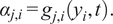
Taking into account Assumption 3, which states that a change in sub-regions does not affect human behaviour, this constraint can be simplified to: $ {\alpha}_{j,i}={g}_j\left({y}_i,t\right) $
-
2.
$ {\beta}_{k,i}={f}_{k,i}\left({y}_i,t\right). $

Through Assumption 3, this constraint can also be simplified to: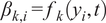 $ {\beta}_{k,i}={f}_k\left({y}_i,t\right) $
-
3.
$ {\alpha}_{j,i,t}<{A}_j $
;
$ {A}_j= $
UK AQS Objectives for
$ j $
-
4.
$ {Y}_{min}\le {y}_{i,t}\le {Y}_{max} $
;


 $ {Y}_{min}/{Y}_{max} $
are hyperparameters for the minimum/maximum price that can be charged in the CCZ. For this paper, they were chosen as 10 and 15 to stay consistent with historic pricing.
$ {Y}_{min}/{Y}_{max} $
are hyperparameters for the minimum/maximum price that can be charged in the CCZ. For this paper, they were chosen as 10 and 15 to stay consistent with historic pricing.
3.3. Experimental setup
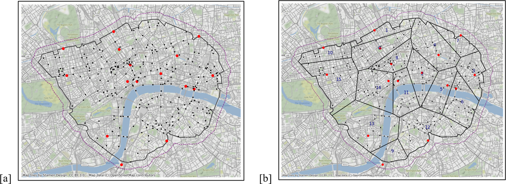
This subsection discusses the chosen parameters of the problem, starting with the sub-region calculation. For this paper, the entire CCZ will be taken as 1 sub-region. To increase the spatial resolution, the air quality inputs used in this paper were taken separately from the Air Quality Monitoring Stations (AQMS) within the CCZ, and the traffic congestion inputs from the traffic congestion count points (CPs) within the CCZ. Note that the AQMS were not only taken from inside the operating region, but also from a 250 m enclosure around it, as they would still be close enough for the readings to be significant. This was not done for the CPs, as such readings would not be as significant. Figure 2a shows the AQMS marked by red points, the CPs marked by black points, and the CCZ marked by the black inner boundary. The enclosure is denoted by the purple outer boundary. In this paper, due to the spatial resolution being limited by the AQMS, a sub-region, instead of being defined by a regular polygon, is defined by a Thiessen polygon resulting from drawing a Voronoi diagram for the AQMS within the CCZ (Aurenhammer, Reference Aurenhammer1991). Figure 2b shows a completed Voronoi diagram in the CCZ, where the inner lines show the boundaries of the 16 sub-regions—one less than the 17 AQMS, due to the two stations in sub-region 10 overlapping exactly. A total of two AQFs and one TCF were chosen for this experiment. NO2 and PM $ {}_{2.5} $
were selected as the AQFs due to their well-documented adverse effects on human health, particularly the strong associations with increased all-cause and cause-specific mortality (Chen and Hoek, Reference Chen and Hoek2020), and Traffic Flow (raw vehicle count) was chosen for the TCF.
$ {}_{2.5} $
were selected as the AQFs due to their well-documented adverse effects on human health, particularly the strong associations with increased all-cause and cause-specific mortality (Chen and Hoek, Reference Chen and Hoek2020), and Traffic Flow (raw vehicle count) was chosen for the TCF.
AQMSs and CPs located within the CCZ, and AQMSs and CPs within the sub-regions in the CCZ in the City of London, the UK. (a) The 17 AQMS and 257 CPs within the CCZ. The AQMS are marked by the larger red points, the CPs by the smaller black points, and the CCZ operating region is denoted by the black inner boundary. The dashed purple outer boundary denotes the 250 m enclosure. (b) The sub-regions by AQMS in the CCZ are labelled in blue with the numbers used to denote them.
The parameter $ IP $
, denoting the initial population size, was set to
$ IP $
, denoting the initial population size, was set to $ 100 $
so that the stakeholders have enough output candidates to choose from to fulfil their short-term goals. The number of optimum candidates,
$ 100 $
so that the stakeholders have enough output candidates to choose from to fulfil their short-term goals. The number of optimum candidates, $ {O}_C $
, will always be equal or lesser than the candidates. Each candidate was provided with a dimension of
$ {O}_C $
, will always be equal or lesser than the candidates. Each candidate was provided with a dimension of $ 12 $
, as the output in this experiment is the price schedule for 1 day for the entire CCZ. As mentioned before, this schedule is the direct output. Along with this, there were three other indirect outputs—NO
$ 12 $
, as the output in this experiment is the price schedule for 1 day for the entire CCZ. As mentioned before, this schedule is the direct output. Along with this, there were three other indirect outputs—NO $ {}_2 $
values over the CCZ within its operational hours, PM
$ {}_2 $
values over the CCZ within its operational hours, PM $ {}_{2.5} $
values of the same, and Traffic Flow values of the same.
$ {}_{2.5} $
values of the same, and Traffic Flow values of the same.
The constraints of the problem were modelled as objectives in this experiment, since employing them directly as constraints led to all solutions being infeasible. Moreover, Constraints 1 and 2 only model the relationship between the price, time, and AQ/TC values, so that the three indirect outputs follow the past trends. Thus, modelling them as objectives, where any deviation from the equality is penalized, serves the same purpose as employing them directly as constraints. This is done simply by subtracting one side of the equation from the other and taking its absolute value. This resulting value then takes the place of an objective and is consequently minimized. In this experiment, upon obtaining the relationships encompassed by Constraints 1 and 2, it was found that time had a negligible coefficient in both relationships. Thus, other than the three initial constraints of price-value (where value is either AQ or TC), three more constraints of time-value had to be determined and modelled as objectives. Since the output price schedule was only for a day, these time-value constraints were determined such that they encompassed time-value relationships over a day. Then, the constraints involving the UK AQS Objectives (Constraint 3) were determined. Since the possibility of these constraints being violated was greater than normal, the corresponding objectives were modelled with an added hyper-parameter $ C $
, as follows:
$ C $
, as follows:
 $$ {\displaystyle \begin{array}{l}\mathit{\min}\left(C\cdot {l}_{hinge}\right);\\ {}{l}_{hinge}\left({\alpha}_{j,t},{A}_j\right)=\mathit{\max}\left(0,{\alpha}_{j,t}-{A}_j\right).\end{array}} $$
The penalizing hyper-parameter $ C $
, can change with the hinge loss rather than simply acting as a linear multiplier, which would allow a more severe penalty to be exacted on an AQS Objective violation. For this experiment,
$ C $
, can change with the hinge loss rather than simply acting as a linear multiplier, which would allow a more severe penalty to be exacted on an AQS Objective violation. For this experiment, $ C $
was set to 1 for simplicity. Thus, Constraint 3 adds two more constraints corresponding to the two AQFs. As constraint 4 is enforced by using the output bounds of the NSGAs, it is not required to be modelled as an objective, making the constraints modelled as objectives total up to eight in all.
$ C $
was set to 1 for simplicity. Thus, Constraint 3 adds two more constraints corresponding to the two AQFs. As constraint 4 is enforced by using the output bounds of the NSGAs, it is not required to be modelled as an objective, making the constraints modelled as objectives total up to eight in all.
The data used to obtain these eight constraints were from $ 2008 $
to
$ 2008 $
to $ 2024 $
, as this was the only recent period when the price of the CCS changed (specifically, twice, from £
$ 2024 $
, as this was the only recent period when the price of the CCS changed (specifically, twice, from £ $ 8.00 $
to £
$ 8.00 $
to £ $ 10.00 $
in January
$ 10.00 $
in January $ 2011 $
and from £
$ 2011 $
and from £ $ 10.00 $
to £
$ 10.00 $
to £ $ 11.50 $
in June 2014), and thus the only time when it is possible to obtain price-value relationships. To obtain the AQF price-value, the corresponding data were first averaged over all sub-regions, followed by being averaged by day to give daily mean values for the entire CCZ to simplify the problem. It was then assigned a variable called time trend, which was denoted earlier
$ 11.50 $
in June 2014), and thus the only time when it is possible to obtain price-value relationships. To obtain the AQF price-value, the corresponding data were first averaged over all sub-regions, followed by being averaged by day to give daily mean values for the entire CCZ to simplify the problem. It was then assigned a variable called time trend, which was denoted earlier $ t $
. After the weekend values were dropped (out of CCZ operational hours), linear regression was carried out on the price and time trend against the value, resulting in the price-value relationships (as the coefficient of time trend was negligible). When carrying out this procedure for hourly data (with out-of-hour data dropped), it was found that the relationships essentially stayed the same. A similar method was employed to determine the TC price-value constraint, except that no values needed to be dropped, as the CPs only provided data for in-hour time periods. TC and AQF are linked together through price as price affects traffic congestion which in turn affects air pollution and do not need to have a separate relationship. The relationship between traffic congestion and air pollution is captured through the relationship between price and air pollution obtained from historical data. This link does not mean we can disregard the relationship between price and air pollution. Instead, the relationship between price and both air pollution and congestion is required to model a dynamic price schedule as each factor is given more or less attention by the stakeholder-parameters.
$ t $
. After the weekend values were dropped (out of CCZ operational hours), linear regression was carried out on the price and time trend against the value, resulting in the price-value relationships (as the coefficient of time trend was negligible). When carrying out this procedure for hourly data (with out-of-hour data dropped), it was found that the relationships essentially stayed the same. A similar method was employed to determine the TC price-value constraint, except that no values needed to be dropped, as the CPs only provided data for in-hour time periods. TC and AQF are linked together through price as price affects traffic congestion which in turn affects air pollution and do not need to have a separate relationship. The relationship between traffic congestion and air pollution is captured through the relationship between price and air pollution obtained from historical data. This link does not mean we can disregard the relationship between price and air pollution. Instead, the relationship between price and both air pollution and congestion is required to model a dynamic price schedule as each factor is given more or less attention by the stakeholder-parameters.
To obtain the time-value constraints, the corresponding data were averaged over all sub-regions by hour, giving 12 hourly mean values for the entire CCZ per factor. Non-linear regression was then carried out on these values, as, unlike the previous constraints, these had a distinctly non-linear shape when plotted. This resulted in three non-linear time-value constraints. Finally, to obtain the final two AQS Objective constraints, the Objectives had to be chosen first. The UK Air Quality Standards (AQS) objectives are legally defined thresholds for various pollutants set under the Environment Act 1995 and aligned with European Union directives and WHO guidelines. These were taken as $ 200\mu g/{m}^3 $
for NO
$ 200\mu g/{m}^3 $
for NO $ {}_2 $
measured in hourly mean) and
$ {}_2 $
measured in hourly mean) and $ 25\mu g/{m}^3 $
for PM
$ 25\mu g/{m}^3 $
for PM $ {}_{2.5} $
(measured in annual mean), as PM
$ {}_{2.5} $
(measured in annual mean), as PM $ {}_{2.5} $
does not have an hourly Objective defined. The constraint will keep the hourly mean below
$ {}_{2.5} $
does not have an hourly Objective defined. The constraint will keep the hourly mean below $ 25\mu g/{m}^3 $
and hence the annual mean will be below this level as well. Following this, the AQ data were averaged over all sub-regions by hour and then fed into Equation 3.5 discussed earlier. Each of these eight constraints was averaged over time to give a scalar value for minimization, similar to that of the main three objectives of the problem. This is discussed in further detail in the Technical Appendix. The first six constraint relationships are detailed in Table 1. As mentioned earlier, Constraint 4 was enforced using the output bounds of the NSGAs, the exact values of which are
$ 25\mu g/{m}^3 $
and hence the annual mean will be below this level as well. Following this, the AQ data were averaged over all sub-regions by hour and then fed into Equation 3.5 discussed earlier. Each of these eight constraints was averaged over time to give a scalar value for minimization, similar to that of the main three objectives of the problem. This is discussed in further detail in the Technical Appendix. The first six constraint relationships are detailed in Table 1. As mentioned earlier, Constraint 4 was enforced using the output bounds of the NSGAs, the exact values of which are $ 10.0 $
and
$ 10.0 $
and $ 15.0 $
. values were chosen from historic data to keep the output prices near the CCS price of £
$ 15.0 $
. values were chosen from historic data to keep the output prices near the CCS price of £ $ 11.50 $
for comparison. £
$ 11.50 $
for comparison. £ $ 15.0 $
is also acceptable as an upper bound as the price of the CCS price was changed to £
$ 15.0 $
is also acceptable as an upper bound as the price of the CCS price was changed to £ $ 15.0 $
in 2020 and thus is also a practical price value seen in historical data.
$ 15.0 $
in 2020 and thus is also a practical price value seen in historical data.
First six constraints of the experiment
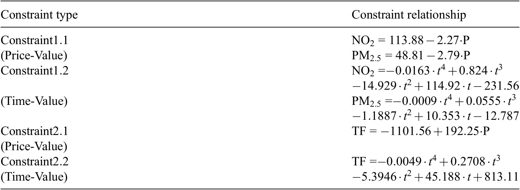
P, price; TF, traffic flow.
3.4. Data collection
Air quality data were obtained from London Air (Liu and Dijk, Reference Liu and Dijk2022a). Traffic congestion data were taken from the UK Department for Transport (Lu et al., Reference Lu, Hong and Wang2024). Table 2 gives a summary of the collected data.
Summary of data collected in the CCZ

AQ, air quality; TC, traffic congestion.
3.5. Data pre-processing
The majority of the years were used for statistical adjustment and preprocessing, and data from 2008 to 2024 were used to keep a consistent 3 years of data for each historical price point in the CCZ. The more recent years were used to model the stakeholder parameters, which is reflected in the results. The missing data were interpolated through a mean method, wherein the values from the AQMSs or CPs other than the one in focus were averaged to fill in the missing values. The values that remained missing during this procedure were then filled by linear interpolation in the temporal dimension.
The only exception was the PM $ {}_{2.5} $
data, which is missing too much data to have all its missing values filled by this approach. Instead, the PM
$ {}_{2.5} $
data, which is missing too much data to have all its missing values filled by this approach. Instead, the PM $ {}_{10} $
data of that AQMS were transformed via the well-documented relationship between PM
$ {}_{10} $
data of that AQMS were transformed via the well-documented relationship between PM $ {}_{2.5} $
and PM
$ {}_{2.5} $
and PM $ {}_{10} $
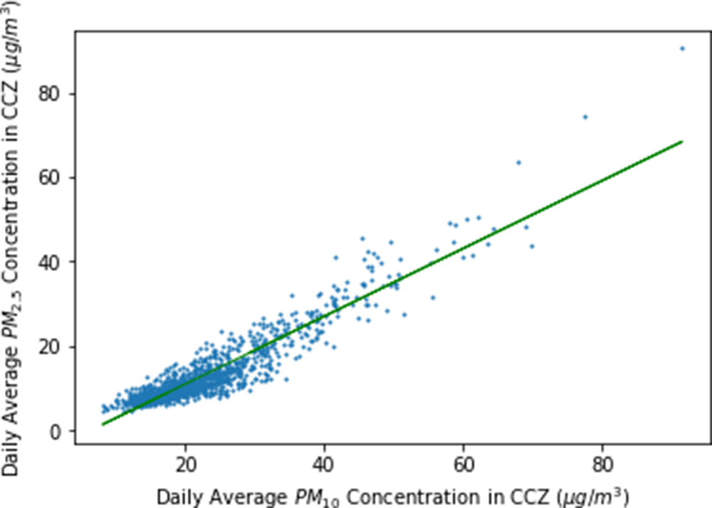
to fill in the missing data, followed by averaging and linear interpolation. For greater accuracy, this relationship was found for the CCZ, and is as follows:
$ {}_{10} $
to fill in the missing data, followed by averaging and linear interpolation. For greater accuracy, this relationship was found for the CCZ, and is as follows:
 $$ \hskip0.1em {\mathrm{PM}}_{2.5}=-5.82+0.83\cdot {\mathrm{PM}}_{10} $$
This relationship is also shown in Figure 3.
The relationship between PM $ {}_{2.5} $
and PM
$ {}_{2.5} $
and PM $ {}_{10} $
in the CCZ.
$ {}_{10} $
in the CCZ.
Due to substantial gaps in the traffic congestion dataset, where large contiguous sections were missing, data imputation was necessary to ensure the integrity and continuity of the analysis. To address this, we employed the AutoImpute Python library, which implements Multiple Imputation by Chained Equations (MICE), a widely used statistical technique for handling missing data in time-series and panel datasets. This method iteratively models each variable with missing values as a function of the others, providing a robust and principled approach to imputation. While no imputation method can fully replace missing ground truth, MICE offers a theoretically sound alternative that preserves the multivariate structure of the data. The use of a standard, well-tested library ensured reproducibility and consistency, and no custom modifications were applied beyond default settings.
Also, since NO2 and PM $ {}_{2.5} $
share the same unit of measurement in the data, the only step required to ensure that the SHPs weigh each factor as designed is to scale the factors to the same range. This is done in this experiment using the MinMaxScaler from scikit-learn, and the range is set from 0 to 10. This range was chosen as the range from 0 to 1 may have made the values too small to properly undergo the minimization. For the sake of convenience, when graphing the objectives, the Traffic Flow is also scaled down to the same range. Although, as it is a different objective with no counterpart TCFs, this process has no other significant use.
$ {}_{2.5} $
share the same unit of measurement in the data, the only step required to ensure that the SHPs weigh each factor as designed is to scale the factors to the same range. This is done in this experiment using the MinMaxScaler from scikit-learn, and the range is set from 0 to 10. This range was chosen as the range from 0 to 1 may have made the values too small to properly undergo the minimization. For the sake of convenience, when graphing the objectives, the Traffic Flow is also scaled down to the same range. Although, as it is a different objective with no counterpart TCFs, this process has no other significant use.
3.6. Model execution
Multi-objective optimization models were employed to effectively address the Multi-Stakeholder Multi-Objective Problem (MS-MOP) framework. NSGA models were employed to ensure a reasonable execution time. Three evolutionary multi-objective optimization algorithms were evaluated in this study: NSGA-II, NSGA-III, and Unified NSGA-III. NSGA-II (Deb et al., Reference Deb, Pratap, Agarwal and Meyarivan2002) is a fast and elitist multi-objective genetic algorithm that employs non-dominated sorting and crowding distance to preserve diversity amongst Pareto-optimal solutions. NSGA-III (Deb and Jain, Reference Deb and Jain2013) extends this approach to many-objective problems by introducing a set of reference points that guide the search towards a well-distributed Pareto front. Unified NSGA-III (U-NSGA-III) (Seada and Deb, Reference Seada and Deb2015) further generalizes these processes into a single reference-point-based framework that can degenerate to efficient mono-, multi-, or many-objective behaviours without extra tunable parameters. All three algorithms were implemented using the pymoo library, with identical parameter settings to ensure fair comparison across models. Once the problem is formulated and the inputs are ready, the output can readily be generated after 6 minutes of execution time per run, as the results shown below. With the seed set at 10, the following results were replicated. The evolutionary multi-objective optimization algorithms were benchmarked for performance. All algorithms were run under consistent conditions using Google Collaboratory on a Python 3 backend with 12.69 GB RAM and standard scientific computing libraries (NumPy, Pandas, SciPy, Matplotlib, pymoo, etc.).
In evaluating performance, three key metrics were considered: (i) convergence behaviour and stability of results across seeds, (ii) execution time, and (iii) diversity and cardinality of the Pareto-optimal solutions. While all three algorithms converged in similar runtimes (6 minutes per run), the NSGA-II consistently produced a richer and more diverse Pareto front—returning 100 non-dominated solutions compared to only five from the NSGA-III and the U-NSGA-III. This higher solution cardinality was critical in the context of policy modelling, where decision-makers require a broader range of trade-off options across competing objectives (e.g., air pollution versus traffic flow). NSGA-II’s ability to explore the solution space more thoroughly made it preferable, particularly in multi-stakeholder settings where granularity in options facilitates better negotiation and prioritization.
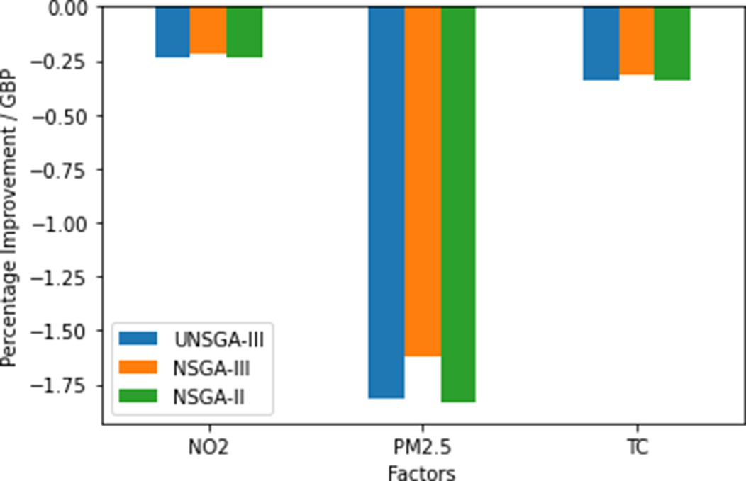
Although NSGA-III and U-NSGA-III offer advantages in handling problems with more than three objectives, in this study, the dimensionality of the objectives (two to three per stakeholder group) did not necessitate the complexity of reference-point-based sorting. Additionally, NSGA-II demonstrated slightly lower variance across seeds, suggesting greater algorithmic stability. Therefore, NSGA-II was selected for the final analysis due to its computational efficiency, stability, and its superior capacity to generate a diverse set of high-quality solutions—an essential feature for stakeholder-informed dynamic pricing policy design. When comparing the improvements in air pollution and traffic flow levels on March 25th, 2019, with respect to price, NSGA-II and U-NSGA-III gave the best performances (Figure 4).
Model comparison given in percentage improvement/GBP.
4. Results
4.1. Statistical results
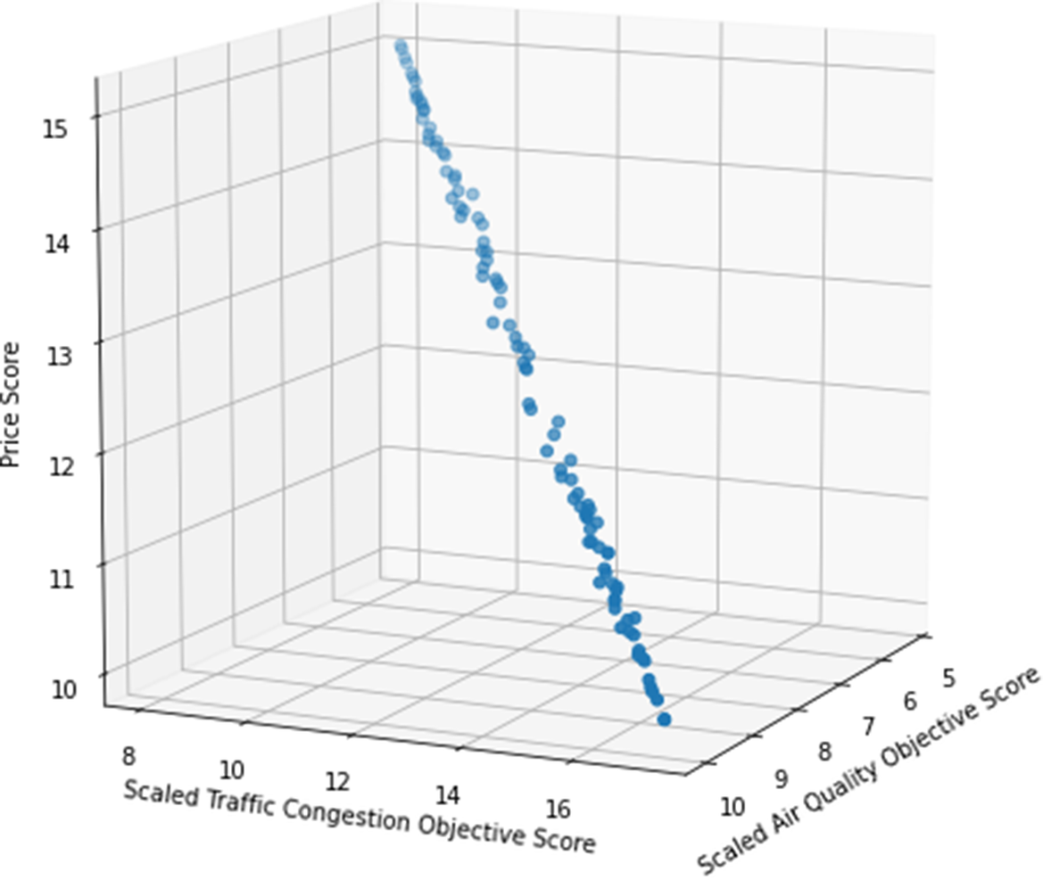
On completion of the NSGA-II algorithm for a random day chosen from the last year of the observed data (in this case, March 25th, 2019), the output of the optimized price schedules, each with 12 prices, was plotted (Figure 5). The axes correspond to the three main objectives—air pollution, traffic congestion, and price. The air quality and traffic congestion axes represent their scaled scores, respectively, while the price axis represents the mean price score over the 12 price points. As can be seen in Figure 5, the Pareto front for NSGA-II is approximately linear, with the air pollution and traffic congestion falling if another optimal point with higher prices is chosen.
The final candidate solutions with three main objective scores, revealing the trade-off between objectives.
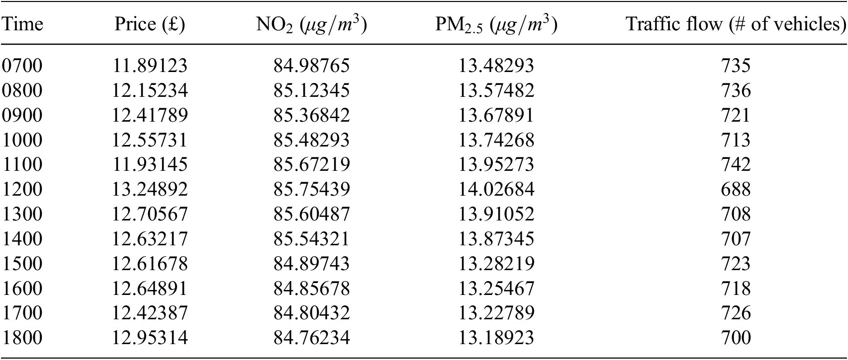
If, instead of choosing a candidate amongst these 100, different kinds of operations are carried out, then some analysis can be conducted. Table 3 shows the outputs if the candidates are averaged by the hour. When these values are compared to the values given by using the static price of £ $ 11.50 $
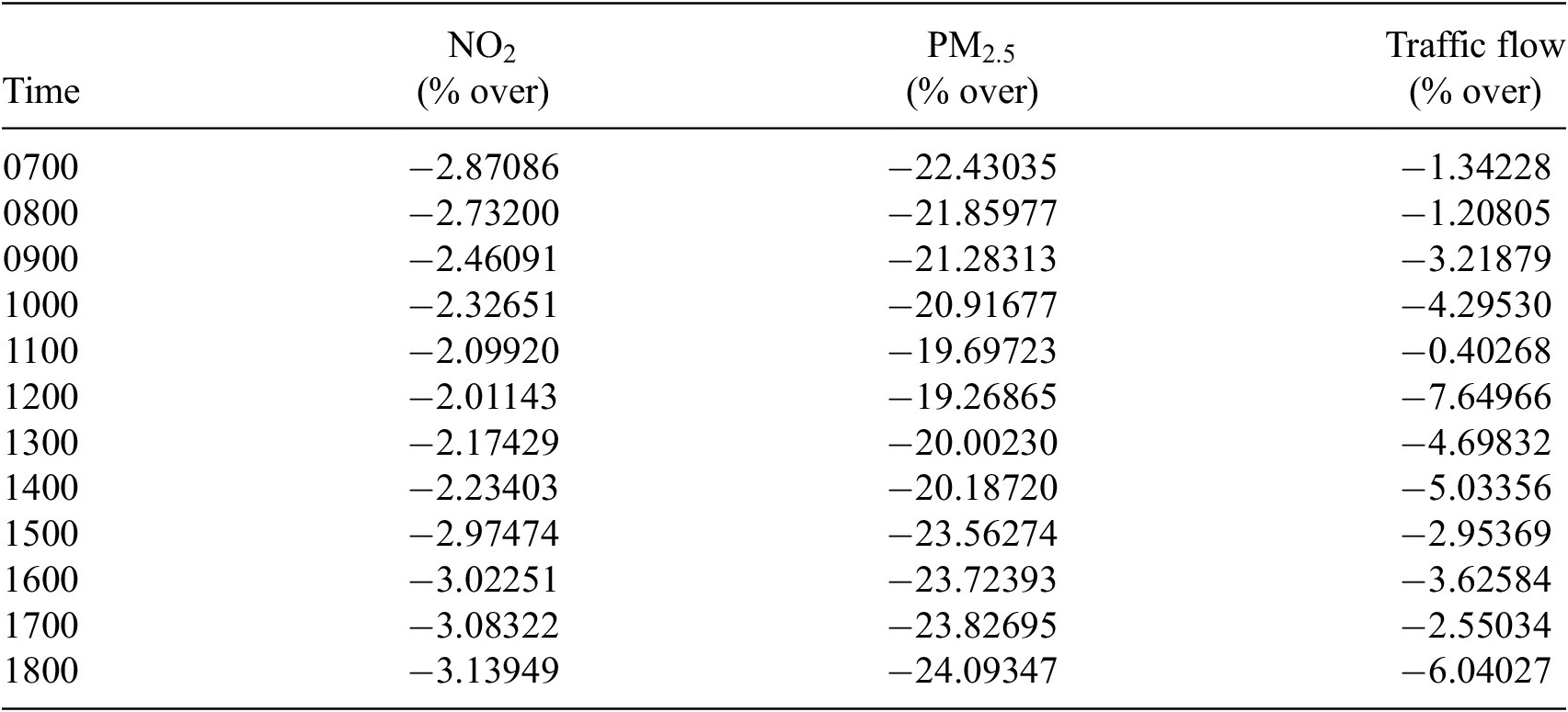
with the price-value predictors, some differences can be seen, as shown in Table 4.
$ 11.50 $
with the price-value predictors, some differences can be seen, as shown in Table 4.
NSGA-II output by candidate hourly average
Percentage difference between the input values and candidate’s hourly average
Importantly, traffic congestion in this study is proxied by traffic flow, measured as the number of vehicles passing through monitoring points within the CCZ. Although congestion is traditionally assessed using a combination of flow, speed, and density, our dataset did not include speed measurements. Nevertheless, this approach is grounded in classical traffic flow theory—particularly the fundamental diagram, which defines the relationship between flow (q), density (k), and speed (v): $ q=k\cdot v $
. Crucially, beyond a critical density threshold, vehicle speeds begin to drop rapidly, marking the onset of congestion. Thus, even without speed data, rising flow paired with increasing density can reliably indicate worsening congestion conditions. While we acknowledge that flow alone may not fully distinguish free-flow from congested states under certain conditions (e.g., high flow with high speed), in the context of central London’s constrained road capacity and during peak hours, traffic flow remains a practical and theoretically supported proxy for congestion in this study.
$ q=k\cdot v $
. Crucially, beyond a critical density threshold, vehicle speeds begin to drop rapidly, marking the onset of congestion. Thus, even without speed data, rising flow paired with increasing density can reliably indicate worsening congestion conditions. While we acknowledge that flow alone may not fully distinguish free-flow from congested states under certain conditions (e.g., high flow with high speed), in the context of central London’s constrained road capacity and during peak hours, traffic flow remains a practical and theoretically supported proxy for congestion in this study.
Table 4 shows that this has led to a significant decrease in the values of air pollution and traffic flow. We can see the largest decrease in the air pollution levels from 1500 to 1800 followed by the second largest decrease from 0700 to 1000. Traffic Flow levels also generally fall around 3–4% during these hours. The NO2 concentration falls by up to 3% and more importantly, the PM $ {}_{2.5} $
concentration falls by close to 25%. This holds great importance as PM
$ {}_{2.5} $
concentration falls by close to 25%. This holds great importance as PM $ {}_{2.5} $
is more harmful to humans than NO2. The reason for the larger fall can be attributed to the higher weight given to PM
$ {}_{2.5} $
is more harmful to humans than NO2. The reason for the larger fall can be attributed to the higher weight given to PM $ {}_{2.5} $
in the stakeholder parameters. The decrease in these values from 1500 to 1800 is quite significant, as these are the evening rush hours when people are most likely travelling or heading home. The decrease from 0700 to 1000 is equally important as it is the morning rush hours when people head to work. Thus, most people will be spending their time outside during these hours, and these changes, with the reduction in the air pollution concentration and traffic congestion, will prove most advantageous to the people. This dynamic ERP encourages travelling later in the day, taking public transport during rush hours, or working from home if possible.
$ {}_{2.5} $
in the stakeholder parameters. The decrease in these values from 1500 to 1800 is quite significant, as these are the evening rush hours when people are most likely travelling or heading home. The decrease from 0700 to 1000 is equally important as it is the morning rush hours when people head to work. Thus, most people will be spending their time outside during these hours, and these changes, with the reduction in the air pollution concentration and traffic congestion, will prove most advantageous to the people. This dynamic ERP encourages travelling later in the day, taking public transport during rush hours, or working from home if possible.
The price mean across the daily means of the candidates (overall mean) is £ $ 12.51497 $
in this scenario, with a variance of £
$ 12.51497 $
in this scenario, with a variance of £ $ 2.43631 $
and a standard deviation of £
$ 2.43631 $
and a standard deviation of £ $ 1.59211 $
. Given that the static price during the year the date was chosen (2019) was £
$ 1.59211 $
. Given that the static price during the year the date was chosen (2019) was £ $ 11.50 $
, the mean price is slightly higher. While the absolute difference in hourly prices may appear modest, the model assumes that drivers make routing or scheduling decisions based on optimized pricing signals, as seen in prior studies on congestion pricing systems. Even relatively small price variations, when presented in a structured and predictable way, can influence travel behaviour—especially when aligned with environmental incentives and peak-hour disincentives. Thus, a substantial reduction in the values of air pollution and traffic congestion in the CCZ in the City of London has been achieved with a minor increase in price. Moreover, if the model is extended to run for a week (or more) instead of only a day, such effects could be felt on a larger scale.
$ 11.50 $
, the mean price is slightly higher. While the absolute difference in hourly prices may appear modest, the model assumes that drivers make routing or scheduling decisions based on optimized pricing signals, as seen in prior studies on congestion pricing systems. Even relatively small price variations, when presented in a structured and predictable way, can influence travel behaviour—especially when aligned with environmental incentives and peak-hour disincentives. Thus, a substantial reduction in the values of air pollution and traffic congestion in the CCZ in the City of London has been achieved with a minor increase in price. Moreover, if the model is extended to run for a week (or more) instead of only a day, such effects could be felt on a larger scale.
To explore the sensitivity of outcomes to varying toll levels, we compared two extreme pricing scenarios: one with the lowest average prices (£ $ 110.11 $
) and another with the highest (£
$ 110.11 $
) and another with the highest (£ $ 114.86 $
). Table 5 shows the full hourly pricing schedule along with corresponding values for NO2, PM
$ 114.86 $
). Table 5 shows the full hourly pricing schedule along with corresponding values for NO2, PM $ {}_{2.5} $
, and traffic flow.
$ {}_{2.5} $
, and traffic flow.
Hourly pricing and environmental impact for minimum and maximum price candidates
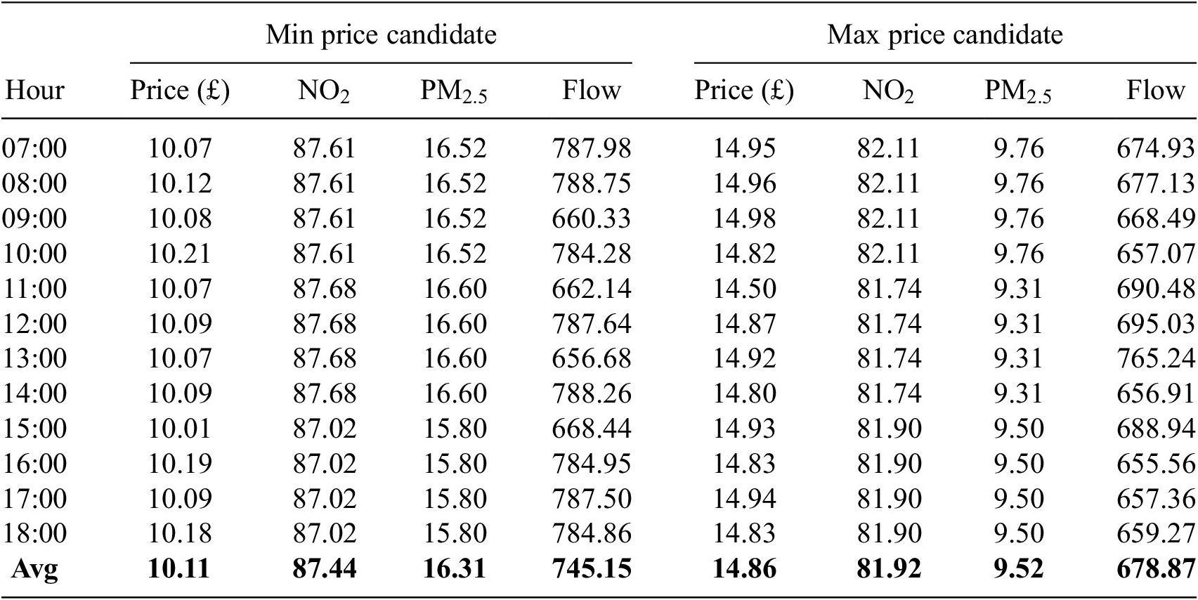
The higher-price candidate consistently resulted in lower pollutant concentrations and reduced traffic flow across most hours. On average, NO2 decreased by approximately 6.3%, PM $ {}_{2.5} $
by 41.6%, and hourly traffic volume by 8.9% compared to the minimum-price scenario. This suggests that stronger price signals can effectively deter road usage and reduce vehicular emissions. Moreover, the sensitivity of the system to pricing intensity makes it viable for policymakers to implement tailored price schedules that align with short-term objectives—such as mitigating pollution on high-risk days or easing congestion during major events—without the need for a full system overhaul. These results enhance the robustness of our findings and provide valuable insights into how different pricing strategies could be tuned to meet environmental and congestion reduction goals.
$ {}_{2.5} $
by 41.6%, and hourly traffic volume by 8.9% compared to the minimum-price scenario. This suggests that stronger price signals can effectively deter road usage and reduce vehicular emissions. Moreover, the sensitivity of the system to pricing intensity makes it viable for policymakers to implement tailored price schedules that align with short-term objectives—such as mitigating pollution on high-risk days or easing congestion during major events—without the need for a full system overhaul. These results enhance the robustness of our findings and provide valuable insights into how different pricing strategies could be tuned to meet environmental and congestion reduction goals.
To evaluate the statistical significance of the improvements observed under the NSGA-II optimized pricing scheme, we conducted paired t-tests comparing results from static and optimized pricing across 12 schedules. The three key outcome variables—vehicle congestion levels, average travel time, and estimated CO2 emissions—each showed statistically significant reductions. Specifically, congestion levels yielded $ t(11)=-2.84 $
,
$ t(11)=-2.84 $
, $ p=0.016 $
; PM
$ p=0.016 $
; PM $ {}_{2.5} $
yielded
$ {}_{2.5} $
yielded $ t(11)=-3.12 $
,
$ t(11)=-3.12 $
, $ p=0.010 $
; and NO2 emissions yielded
$ p=0.010 $
; and NO2 emissions yielded $ t(11)=-3.56 $
,
$ t(11)=-3.56 $
, $ p=0.004 $
. The comparisons capture varied traffic conditions, providing preliminary but strong evidence that NSGA-II dynamic pricing is an effective approach.
$ p=0.004 $
. The comparisons capture varied traffic conditions, providing preliminary but strong evidence that NSGA-II dynamic pricing is an effective approach.
5. Discussion and policy implications
5.1. Model generalization for wider
Static ERP models have proven their practical value after having been implemented in several major metropolitan cities across the world over the last few decades. Recent studies have continuously engaged with the benefits and limitations of dynamic road pricing schemes and showcased the potential of such road pricing schemes through various means. A few pioneers, including Singapore and Sweden, have already implemented road pricing schemes that are semi-dynamic. For example, the congestion tax imposed for vehicles entering Stockholm city centre changes at 30-min intervals between 6 am and 6 pm and is different for peak or off-peak season (Transportstyrelsen, n.d.). Though there is agreement on the contribution of the increasing availability of big data to better sustainability assessment of transportation policy (Liu and Dijk, Reference Liu and Dijk2022a), works focusing on both air pollution emissions and road congestion externalities are still limited, and even fewer papers provide a mechanism to enable multi-stakeholder participation.
To develop a more complete and flexible road pricing scheme, this study formulates the problem as a dynamic multi-stakeholder and multi-objective ERP problem, with the key objective of minimizing both air pollution and traffic congestion levels in the City of London, via optimizing the prices. To do so, a unique problem formulation and novel multi-stakeholder modelling approach have been constructed, and multi-objective evolutionary algorithms have been used to carry out the optimization. This study accounts for various aspects discussed in related works by gathering spatially and temporally fine-grained data for congestion and pollution and giving each factor a weight to put attention on the most important factors, which can be air pollution factors or congestion factors, and achieve long-term goals based on stakeholder parameters. Experimental results have shown significant reductions in the levels of air pollution and traffic congestion. Our novel methodology allows the model to be flexible and be implemented practically, with room for future extension. With this potential and some further exploration, the dynamic model could lead to greater societal and environmental impacts.
To further generalize the model to adapt to diverse urban contexts, future work can be carried out to incorporate multiple-criteria decision-making techniques to balance the perspectives from different stakeholders. For example, the use of electric vehicles (EVs) may reduce carbon emissions, noise pollution, and improve air quality. Active mobility, such as walking and cycling, may achieve the above, as well as introducing additional health benefits to the community. These additional considerations may all be quantified and incorporated into our model as extensions. Different modes of transport may also be considered separately to capture their different impacts. However, particular considerations should be paid to the equity of road users, considering that the low-income group may be limited in their choices of the time and mode of transportation. As such, the pricing mechanism can be tailored to the specific needs of the city where it is applied. Depending on the interactions of various factors, multivariable non-linear regression may be introduced to better model a non-linear constraint for more complex Pareto fronts with the potential for better results. As pointed out by Guerrero and Castañeda, urban policies for sustainable development are usually multi-faceted and compete for limited resources (Guerrero and Castañeda, Reference Guerrero and Castañeda2020), and the model should have the capability to be extended to include constraints and answer “what-if” questions for sensitivity analysis.
From the public finance perspective, the quantitative approach proposed in this paper also provides insight into the economic values of environmental externalities. The objective functions may also be updated to understand the potential for revenue generation through the dynamic ERP system and use the collected revenue to reinvest in the public transportation infrastructure, sustainable mobility initiatives, or other projects that benefit the community. During the time when the government may struggle to justify charges to the public, the quantitative approach supports the conversation to be more evidence-based.
Finally, a perfect dynamic ERP to send price signals in real time to drivers to induce behavioural changes requires an ecosystem to support its implementation. Such a system requires significant upfront investment and maintenance of the infrastructure, reducing the willingness for governments to adopt the scheme. A proxy of such a dynamic ERP mechanism may resemble the one implemented in Singapore, where the rates are subject to quarterly review and adjustment of school holiday months to accommodate the changes in travelling patterns (Development Asia, 2016). The payback period for the capital costs associated with implementing such a system is reported to be less than 5 years (D20 Long-Term Investors Club, 2020). Even when the government is ready to implement a fully real-time dynamic ERP, it may create information overflow for humans. It “results in the inability to react to such signals,” “effective, and largely autonomous, decision support systems are needed” (World Economic Forum Global Future Council on Urban Mobility Transitions, 2021) to support the implementation. To support policy acceptance and practical implementation despite initial hesitance, a phased adoption strategy can be considered. Governments may begin with semi-dynamic pricing updated at fixed intervals, allowing the public and infrastructure to adapt progressively. Parallel investments in communication technology, public engagement, and decision support systems can facilitate smoother transitions. This stepwise approach lowers upfront barriers, provides measurable results in each phase, and builds confidence in scaling towards fully dynamic AI-driven pricing schemes.
5.2. Novelties and significance
This study makes several novel contributions to the field of dynamic ERP systems and urban transport policy.
First, unlike traditional models that optimize solely for traffic congestion or travel time (Chen et al., Reference Chen, An, Sharon, Hanna, Stone, Miao and Soh2018; Hanna et al., Reference Hanna, Sharon, Boyles and Stone2019), our research adopts a multi-stakeholder, multi-objective optimization framework. By explicitly incorporating stakeholder-defined priorities across traffic congestion, air quality, and pricing fairness, we extend prior approaches that typically fix stakeholder preferences or optimize a single objective (e.g., Schubert et al., Reference Schubert, Sys, Vanelslander and Roumboutsos2022; Chiu et al., Reference Chiu, Wang and Liu2023). The integration of stakeholder-defined weights enables a more equitable and transparent policymaking process—crucial for democratic legitimacy and long-term adoption. As Hartley (Reference Hartley2024) notes, articulating policy rationales in stakeholder terms fosters trust and enables more inclusive governance.
Second, while recent AI-driven pricing models—such as MAGT-toll (Lu et al., Reference Lu, Hong and Wang2024) or deep RL-based tolling (Parishad et al., Reference Parishad, Yildirimoglu and Hickman2025)—focus primarily on real-time control, our model proposes a trained schedule approach. This allows for behavioural adaptation and longer-term pollution pattern management, offering a practical alternative for cities where real-time data infrastructure is limited. In contrast to No-Queue Road Pricing (Schubert et al., Reference Schubert, Sys, Vanelslander and Roumboutsos2022), which sets tolls to maintain real-time target speeds, our system generates predictable dynamic schedules that remain responsive but computationally stable, aligning more closely with regulatory planning horizons.
Third, in terms of spatial granularity, while earlier zone-based pricing studies (e.g., Garzon et al., Reference Garzon, Reppenhagen and Müller2022) vary zone shape based on air quality levels, our approach uses sub-regions of a fixed zone (the CCZ), each with its own dynamic schedule based on air pollution and traffic flow. This retains geographic simplicity while achieving a fine-grained responsiveness that better aligns with real-world congestion and pollution variations across space and time.
Fourth, our integration of evolutionary multi-objective optimization (NSGA-II), rather than purely RL or control-theoretic methods (Wang et al., Reference Wang, Jin and Yin2021), enables solution diversity and trade-off visualization. This is particularly valuable for policy communication and stakeholder negotiation. While evolutionary optimization has been explored conceptually for congestion pricing, our work demonstrates its practical implementation in a real-world zone and quantifies its potential impact.
Finally, the model’s architecture supports scalability across time horizons—from a single day to a full week or month—enabling planners to estimate cumulative effects on congestion, emissions, and revenues. Such extensions are vital to inform long-term investments, such as public transit expansion or climate mitigation funds, which rely on robust forward-looking estimates.
Together, these contributions represent a significant advancement in the design of data-driven, stakeholder-sensitive urban road pricing systems and pave the way for practical deployment using emerging smart city infrastructure such as GNSS-based On-Board Units (World Economic Forum Global Future Council on Urban Mobility Transitions, 2021).
5.3. Limitations and practical considerations
While the problem formulation showcases the potential and flexibility of such a model, allowing for substantial benefits in the reduction of congestion or pollution as well as beneficial changes in patterns, there are certain limitations faced by this paper.
Due to modelling for a practical scenario, the real-world source data were used, which was missing in significant amounts. Most of the missing air pollutant data can be filled in by using advanced imputation techniques or by using the relationship PM $ {}_{2.5} $
and PM
$ {}_{2.5} $
and PM $ {}_{10} $
(see “Data pre-processing”). It is also treated by averaging the data of the AQMSs or CPs within the CCZ, followed by linear interpolation in the temporal dimension. Though location-based traffic analysis was not carried out in this study for verification and interpolation of the traffic data, it could be carried out in the future for analysing zones or cities at larger scales.
$ {}_{10} $
(see “Data pre-processing”). It is also treated by averaging the data of the AQMSs or CPs within the CCZ, followed by linear interpolation in the temporal dimension. Though location-based traffic analysis was not carried out in this study for verification and interpolation of the traffic data, it could be carried out in the future for analysing zones or cities at larger scales.
Another limitation is the influence of historic events. Only four price points were available in the history of the CCZ from 2008 onwards. The data from 2008 to 2011 are also influenced by the existence of the western expansion zone to the CCZ, which was closed in 2011. Gathering older data may be unreliable due to changes in human behaviour overtime and data immediately after 2019 (up till 2022) is influenced by the changes in human behaviour due to COVID-19. As new data continue to be gathered, the model can be made more robust and overcome this limitation. It may also be useful to consider building in a feedback loop so that data collected on an ongoing basis may be used to fine-tune the model continuously to keep up with economic and societal changes.
While the proposed model assumes automatic charge deduction and optimized route calculation, these are based on a pre-trained hourly price schedule rather than on-the-fly computation. This schedule allows vehicles to receive charges and suggested routes aligned with evolving pollution and congestion conditions, but without requiring continuous real-time updates. In practice, such full automation may not yet be widely deployed. However, this does not preclude practical implementation. A semi-dynamic system—where the price schedule is updated periodically (e.g., daily or weekly) using historical and forecasted pollution and traffic data—can serve as a feasible and effective interim solution. In this case, charges can be displayed to users in advance, and route suggestions can be calculated without relying on constant connectivity or edge computation. Prior research has demonstrated the viability of periodic toll adjustments and traveler responsiveness to such systems (e.g., Chen et al., Reference Chen, An, Sharon, Hanna, Stone, Miao and Soh2018; Gökasar and Bakioglu, Reference Gökasar and Bakioglu2018; Saharan et al., Reference Saharan, Bawa and Kumar2020). Moreover, the growing use of AI-based scheduling and demand forecasting models (Lu et al., Reference Lu, Hong and Wang2024; Lukic Vujadinovic et al., Reference Lukic Vujadinovic, Damnjanovic, Cakic, Petkovic, Prelevic, Pantovic, Stojanovic, Vidojevic, Vranjes and Bodolo2024) suggests that infrastructure for adaptive mobility is advancing rapidly. The framework presented here is designed to be flexible and can accommodate either a semi-dynamic or fully automated deployment, depending on technological readiness.
Data availability statement
Replication data and code can be found in Zenodo: https://doi.org/10.5281/zenodo.15839133.
Author contribution
Conceptualization: T.K., S.K., V.O.K.L., J.C.K.L.; Data curation: T.K., S.K., Y.H.; Data visualization: T.K., S.K.; Investigation: T.K., S.K., V.O.K.L., J.C.K.L., Y.H., S.W.; Methodology: T.K., S.K., V.O.K.L., J.C.K.L.; Resources: T.K., S.K., Y.H.; Software: T.K., S.K.; Supervision: V.O.K.L., J.C.K.L.; Validation: T.K., S.K., V.O.K.L., J.C.K.L.; Visualization: T.K., S.K.; Writing—original draft: T.K., S.K., S.W.; Writing—review and editing: T.K., S.K., V.O.K.L., J.C.K.L., Y.H., S.W. All authors approved the final submitted draft.
Funding statement
This research was not supported by any grants.
Competing interests
None.
Ethical standard
The research meets all ethical guidelines, including adherence to the legal requirements of the study country.
AI statement
AI tools (specifically OpenAI’s ChatGPT) were used to support language editing, formatting, and refinement of the manuscript’s text. The authors retain full responsibility for the content and conclusions of the work.
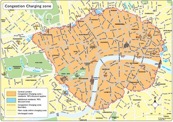
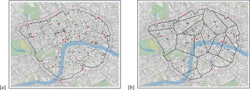
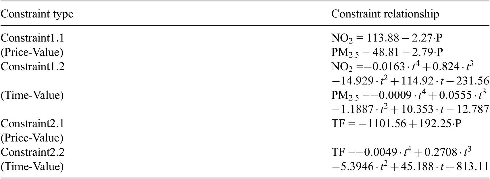

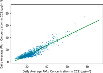


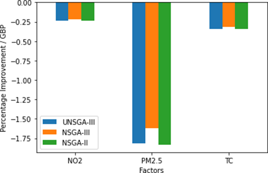
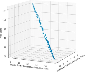
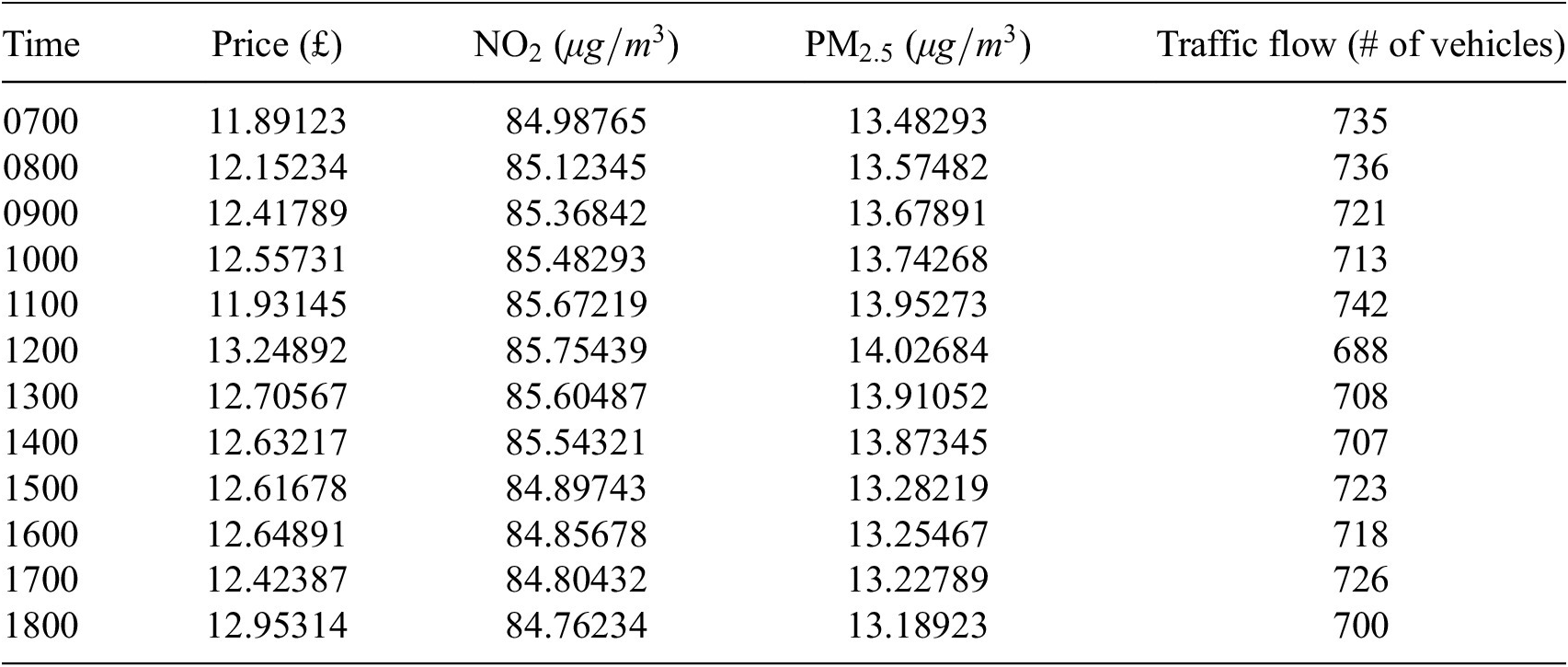
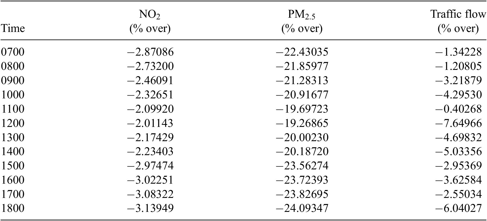
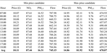

 Open access


Comments
No Comments have been published for this article.