


1. Introduction
The pressure signatures of turbulent boundary layers on underlying surfaces are under active study for their relevance to structural vibrations and noise. For example, the pressure fluctuations determine the source terms for the far-field noise produced by the flow past an aerofoil trailing edge. Similarly, the low wavenumber components of the pressure spectrum determine the structural vibrations and noise in an aircraft or marine vehicle (Blake Reference Blake2017). Fundamentally, pressure fluctuations on the surface are an integrated effect of the turbulent velocity field across the boundary layer, as seen from the solution to the incompressible pressure Poisson equation
 \begin{equation} p(\boldsymbol{x},t) ={-}\frac{\rho}{2{\rm \pi}} \oint_V \left[2\,\frac{{\partial} \overline{U_i}}{{\partial} x_j}\, \frac{{\partial} u_j}{{\partial} x_i} + \frac{{\partial} }{{\partial} x_i x_j} \left( u_iu_j - \overline{u_iu_j}\right)\right]_{(\boldsymbol{y}, t)} \frac{{\rm d} V (\boldsymbol{y})}{|\boldsymbol{x} - \boldsymbol{y}|}. \end{equation}
The fluctuating pressure at a point  $\boldsymbol {x}$ on the surface depends on a complex combination of the mean flow ( $U_i, \overline {u_iu_j}$, where $i,j=1,2,3$) and turbulent fluctuations ( $u_i$) in the boundary layer, weighted by the inverse of the distance from the surface $|\boldsymbol {x}-\boldsymbol {y}|$. The first term of the integrand incorporates the mean velocity gradient and is thought to respond immediately to changes in the mean flow, therefore known also as the rapid term. The second term is nonlinear in the fluctuating velocity and is known as the slow term as it is thought to respond indirectly to changes in the mean flow as it modifies the convective turbulence. Substantial efforts over the past few decades, directed at the canonical case of a planar, zero pressure gradient (ZPG) flow, have lead to an improved understanding of the wall-pressure mechanisms, and consequently well-accepted models for the wall-pressure spectrum (Goody Reference Goody2004) and the full wavenumber–frequency spectrum (Corcos Reference Corcos1964; Chase Reference Chase1980; Smol'yakov Reference Smol'yakov2006). Some outstanding issues such as the lack of consensus in the acoustic and sub-convective ranges of the wavenumber–frequency spectrum require very carefully designed experiments and expensive simulations, and are beginning to be addressed.
For axisymmetric bodies, the effect of lateral curvature on pressure fluctuations has been studied briefly by considering axial flow past a circular cylinder. The importance of lateral curvature on the flow and therefore the wall pressure has been characterized by two parameters:  $\delta /r_s$, which measures the boundary layer thickness ( $\delta$) relative to the radius of curvature of the surface ( $r_s$), and $r_s^+ = r_su_{\tau }/\nu$, the curvature Reynolds number, where $u_\tau$ is the friction velocity, and $\nu$ is the dynamic viscosity. Flows with low $\delta /r_s$ and high $r_s^+$ that represent a high-Reynolds-number flow over a large cylinder (Piquet & Patel Reference Piquet and Patel1999) that represents vehicle-relevant conditions are of interest here. In this case, previous studies (see Snarski & Lueptow Reference Snarski and Lueptow1995) have shown that while mean velocity profiles are fuller and skin friction is higher compared to the flat-plate case, the fundamental turbulence mechanisms in terms of the production and transport are similar. In an early experimental study by Willmarth & Yang (Reference Willmarth and Yang1970), the space–time structure of the wall pressure was examined on an axial cylinder with $\delta /r_s = 2$ and $r_s^+ = 4500$, and they observed that the wall-pressure spectrum was almost similar to the flat-plate case with consistent mean-square levels, except for the slightly amplified high-frequency region ( ${\sim }2$ dB for $\omega \delta _1/U_e > 10$) that was compensated by the weakened low-frequency fluctuations. This shift towards the high-frequency content is consistent with their observation of a shorter correlation length scale in both the longitudinal and lateral directions, suggesting that the pressure-producing motions are located closer to the wall than in the planar case. However, instead of observing the convection velocity to be correspondingly smaller, they observed it to be similar to the flat-plate case. This prompted them to suggest that the pressure-producing motions are smaller and located closer to the wall, but convected at equivalent speeds due to the fuller mean velocity profiles for the cylinder flow. For flows with higher curvature, the flow regime corresponds to that of a long slender rod, relevant to towed-array sensor systems, and the corresponding impact on the wall pressure is more severe; see Willmarth et al. (Reference Willmarth, Winkel, Sharma and Bogar1976), Neves & Moin (Reference Neves and Moin1994) and Bokde, Lueptow & Abraham (Reference Bokde, Lueptow and Abraham1998).
Pressure fluctuations in axisymmetric boundary layers under mean pressure gradient are much more complex and have not been investigated, to the authors’ knowledge. The impact of pressure gradient even on planar boundary layer flows is inherently complex as the flow is sensitive to the pressure-gradient history in addition to the local conditions, posing a prohibitively large parameter space. In an early experimental study of mild adverse pressure gradient (APG) flow, Schloemer (Reference Schloemer1966) observed an increase in the low-frequency spectrum, with a corresponding net increase in the mean-square energy relative to a ZPG layer at otherwise similar conditions. Examining the space–time correlations, they observed that the convection velocity, at similar non-dimensional separations and frequencies, was smaller than the ZPG case as a result of larger velocity defect throughout the boundary layer, which is consistent with the findings of Bradshaw (Reference Bradshaw1967). For stronger APG flows approaching separation, Simpson, Ghodbane & McGrath (Reference Simpson, Ghodbane and McGrath1987) observed the mean-square energy to increase monotonically, scaling with the maximum turbulent shear stress in the outer region, as opposed to  $\tau _w$ for ZPG layers (Bull Reference Bull1996). However, as summarized by Cohen & Gloerfelt (Reference Cohen and Gloerfelt2018), much of the early experimental work is reliable only in the low-frequency regions due to large diameter transducers that suffered from inadequate spatial resolution, preventing an accurate estimation of the higher frequency content.
More recent work investigating the fluctuations in planar APG boundary layers has considered a wider range of configurations, including non-equilibrium flows over aerofoils and wedges (Rozenberg, Robert & Moreau Reference Rozenberg, Robert and Moreau2012; Catlett et al. Reference Catlett, Anderson, Forest and Stewart2015; Kamruzzaman et al. Reference Kamruzzaman, Bekiropoulos, Lutz, Würz and Krämer2015; Hu & Herr Reference Hu and Herr2016; Lee Reference Lee2018). The major focus of these works has been on development of models for the wall-pressure spectrum, by extending Goody's model for ZPG flows (Goody Reference Goody2004). Several parameters have been proposed to accommodate the strength and history of the pressure gradient, generally based on the Clauser's parameter  $\beta _C = (\delta _1/\tau _w) \,{\rm d} p/{{\rm d}x}$, and/or the shape factor $H = \delta _1/\delta _2$. As summarized by Lee (Reference Lee2018), none of the models is universally successful. This is not totally unexpected, since the convective turbulence in the grazing flow – the source of these pressure fluctuations – is not yet fully characterized for pressure-gradient flows. Recently, Grasso et al. (Reference Grasso, Jaiswal, Wu, Moreau and Roger2019) showed that the pressure spectrum for APG flows (obtained from the solution to the Poisson equation) was sensitive to the assumed analytical form of the two-point turbulence. Therefore, the development of well-accepted models requires a systematic study covering a broad range of pressure-gradient histories, examining both the evolution of turbulence and the corresponding wall-pressure spectrum. For the particular case of strong APG flows – the focus of this paper – recent research (Krogstad & Skare Reference Krogstad and Skare1995; Kitsios et al. Reference Kitsios, Sekimoto, Atkinson, Sillero, Borrell, Gungor, Jiménez and Soria2017; Schatzman & Thomas Reference Schatzman and Thomas2017) has suggested a fundamental change in the character of boundary layers that develop inflectional mean velocity profiles in the outer region, which correspond to a secondary peak in the turbulence production and transfer. Examining the conditional velocity structure, the sweep motions were observed to dominate just above the inflection point, while ejections dominated below. Schatzman & Thomas (Reference Schatzman and Thomas2017), through further analysis, suggested the presence of an embedded shear layer with coherent spanwise-oriented vorticity centred about the inflection point. The impact of these findings on the turbulence structure and consequently on the fluctuating wall pressure must be examined.
The object of our research is to provide an understanding of the strong APG axisymmetric boundary layers, in particular of the turbulence structure and the associated wall-pressure fluctuations. The companion paper (Balantrapu et al. (Reference Balantrapu, Hickling, Alexander and Devenport2021), hereafter referred to as BHAD) presents the measurements of the mean flow and turbulence structure of a boundary layer over a body of revolution. BHAD found that the axisymmetric boundary layer behaved as if there is an embedded shear layer in the outer region. Despite being out-of-equilibrium and evolving significantly, the mean velocity and turbulence statistics were self-similar with a free-shear-layer-type scaling, where the velocity defect at the inflection point was the velocity scale, and the vorticity thickness was the length scale. Furthermore, while the large-scale activity in the outer regions energized as the flow decelerated, the spectral distribution of the streamwise velocity was approximately self-similar with the embedded shear-layer scaling, suggesting the importance of the embedded shear-layer motions.
In this paper, we present the associated wall-pressure spectrum and its scaling, along with its relation to the space–time structure. The work is organized as follows. First, we describe the apparatus and instrumentation in § 2. Then we present the results and discussion in § 3, summarizing the flow parameters (§ 3.1) as required to follow the detailed discussion of the wall-pressure spectrum and its scaling in § 3.2. We then describe the associated space–time structure as it relates to the observations made in the wall-pressure spectrum. One principal finding is that the wall-pressure spectrum collapses at all frequencies with the wall-wake scaling, where  $\tau _w$ is the pressure scale, and $U_e/\delta$ is the frequency scale. This broadband success, including the $f^{-5}$ regions, suggests that outer-region motions play a dominant role in near-wall turbulence and wall pressure. In particular, we detect a quasi-periodic feature in the instantaneous wall pressure with a signature similar to that of a roller eddy, and this appears to convect downstream at speeds matching that at the outer peak of the turbulence stresses.
2. Apparatus and instrumentation
The apparatus and instrumentation, except the wall-pressure microphones, are largely similar to those detailed in BHAD and are presented briefly here. All measurements were performed in the anechoic test section of the Virginia Tech Stability Wind Tunnel, designed and documented by Devenport et al. (Reference Devenport, Burdisso, Borgoltz, Ravetta, Barone, Brown and Morton2013). The test section is  $1.85\,{\rm m}\times 1.85\,{\rm m}$ wide and 7.3 m long, and features side walls formed by tensioned Kevlar that contain the flow while remaining acoustically transparent, minimizing the acoustic reflections. Sound passing through the walls is absorbed into anechoic chambers on either side that are lined with acoustic foam wedges, designed to minimize reflections down to 190 Hz. The floor and ceiling are treated similarly with perforated metal panels lined with Kevlar and backed by 0.457 m acoustic foam wedges. Additionally, the entire circuit is treated acoustically to minimize background acoustic reflections (refer to Devenport et al. (Reference Devenport, Burdisso, Borgoltz, Ravetta, Barone, Brown and Morton2013) for a detailed discussion). The free-stream turbulence intensity is significantly low at approximately 0.012 % at 12 m s $^{-1}$, rising gradually to 0.034 % at 57 m s $^{-1}$ as stated in BHAD. These levels are more than three orders of magnitude lower than the turbulence levels seen in the tail boundary layer.
The body of revolution (BOR), shown in figure 1, has characteristic length  $D = 0.4318$ m and a forebody comprised of a 2 : 1 ellipsoid nose joined to a constant-diameter body, each $1D$ long. A $0.8\,{\rm mm}\times 0.8\,{\rm mm}$ ring sandwiched between the nose and centrebody (at $x/D = 0.98$) is used to trip the flow. The aftbody is a 20 $^\circ$ tail cone, forming a sharp corner with the upstream forebody and truncated at 1.172 $D$ downstream to facilitate installation in the test section. Oil flow visualization was performed to verify that the expected separation bubble at the sharp corner was highly local, and that the downstream flow was fully attached to the tail. The BOR is positioned via a hollow sting cantilevered from a vertical post that is 0.91 m downstream from the tail to ensure that the hydrodynamic perturbation was less than 0.5 % of the free-stream velocity $U_\infty$. The sting support was selected as the least intrusive method of mounting the BOR (given that any upstream supports would have contaminated the tail cone flow with their wakes. The effect of the sting on the pressure distribution was small upstream of the tail exit since the measured pressures were in agreement with the panel method calculations (reproduced in figure 3 and detailed in BHAD). While the post was streamlined to a McMasters Henderson aerofoil to mitigate trailing edge shedding (Glegg & Devenport Reference Glegg and Devenport2017), some acoustic contamination was observed in the tail microphones, which was tonal (at approximately 2000 Hz) and excluded by eliminating the signal in that frequency bin with the hydrodynamic content recovered by interpolating across adjacent bins. While the BOR was positioned with the downstream sting, it was suspended in the test section via a cruciform of 0.9 mm tethers running through the centrebody, just downstream of the 0.8 mm trip ring forming clean cylinder–body junctions at the BOR surface. These cruciform tethers are cleated to the internal structure of the BOR, and run diagonally across the test section shown in figure 1. Outside the test section, the tethers are connected to a manual slide on each side of the ceiling and stabilized under the floor by 14.5 kg weights. The characteristics of the tether wake and its highly constrained influence on the BOR boundary layer were discussed in detail by BHAD. However, the acoustic contamination to the surface microphones was tonal at approximately 4500 Hz (corresponding to Strouhal number 0.19) and its harmonics. While this was removed from the wall-pressure spectrum, the discussion in § 3 is limited to frequencies less than 4000 Hz, further ensuring that the disturbance does not impact the results and discussion.

Figure 1. Schematic of the test section, showing the BOR geometry and experimental arrangement.
The BOR was positioned to a  $0 \pm 0.25^\circ$ angle of attack, with the circumferential uniformity in the mean surface pressure confirmed with a ring of pressure taps on the nose, followed by the stagnation pressure measurements at the BOR tail (see figure 6 of BHAD). When positioned at zero angle of attack, the BOR installation poses a 4.3 % blockage in the tunnel. The flow structures on the tail cone were documented extensively, using a combination of hotwire anemometry and particle image velocimetry (PIV). Using a single hotwire, fifteen profiles were obtained, documenting statistics and temporal structure of the streamwise velocity, detailed in § 2.4 in BHAD. While most profiles are not directly above the surface microphones, the flow parameters required to examine the wall-pressure structure are estimated from interpolation due to adequate resolution.
2.1. Fluctuating wall pressure measurements
The fluctuating wall pressure was measured on the BOR tail with a longitudinal array of 15 Sennheiser electret microphones (type KE-4-211-2) spaced linearly. Shown in figure 2, the microphones were installed 67.5 $^\circ$ away from the horizontal (or $\theta = 292.5^\circ$), such that the array was separated circumferentially from the closest tether by approximately 22.5 $^\circ$. This ensured that the microphones were free from any hydrodynamic interference as the wake half-width outside the tail boundary layer ( $x/D=3.172$) was less than 5 $^\circ$ (discussed by BHAD).

Figure 2. Schematic showing the circumferential location of the surface microphones on the tail cone with respect to the tethers. The view corresponds to that seen by an observer located downstream of the BOR and viewing directly upstream.
Figure 3 shows the longitudinal arrangement on the tail against the surface-pressure coefficient distribution and the turbulent kinetic energy (TKE) contours. Microphones were nominally spaced by 12.7 mm arranged between  $x/D=2.53$ to $x/D=3.08$. While more microphones existed upstream ( $x/D=2.0\unicode{x2013}2.5$), unfortunately they were damaged during installation. However, considering that the pressure-gradient effects on the flow are cumulative (Devenport & Lowe Reference Devenport and Lowe2022), the strong pressure-gradient effects persist downstream. Also, note that the blank space in TKE contours was due only to hotwire traverse limitations, and PIV suggested no flow separation in those regions. Each microphone was fitted with a 1 mm pinhole cap, yielding a flat frequency response in the range 50–20 000 Hz. Primary measurements were made at a Reynolds number based on the BOR length, $Re_L=1.92\times 10^{6}$, matching that of the turbulence measurements. Additional wall-pressure measurements were made for a range of Reynolds numbers spanning $1.10\times 10^{6}$ to $2.37\times 10^{6}$. While these are not discussed in the paper due to the absence of turbulence measurements, the wall-pressure spectra and wake velocity profiles had no significant variation, suggesting that the findings of the paper are valid across a broad range of Reynolds numbers. All measurements were made with a 24-bit Bruel & Kjaer LAN-XI acquisition system sampling at 65 536 Hz for 32 seconds, and anti-alias filtered at 25 600 Hz. The one-sided spectral density was estimated using the fast Fourier transform algorithm in MATLAB by segmenting the time series into 511 blocks of 8192 samples in each block, along with a 50 % overlap and Hanning window.

Figure 3. Surface microphone positions, with nominal spacing 12.5 mm, shown against turbulent kinetic energy (TKE) contours. Also shown in green is the mean pressure distribution on the tail, with relevant vertical axis to the right. Dots represent the experimental data, the dashed line shows large eddy simulations estimates from Zhou, Wang & Wang (Reference Zhou, Wang and Wang2020), and crosses show the potential flow simulation.
3. Results and discussion
Results are discussed in the coordinate system  $(x,y,z)$ centred at the BOR nose, as shown earlier in figure 1, where $x$ is along the axis of symmetry or the approach flow, the $y$-axis points vertically upwards, and the $z$-axis completes a right-handed system. In the corresponding cylindrical coordinate system $(x,r,\theta )$, $r$ is the radial distance from the $x$-axis, and $\theta$ is the polar angle, measured from the vertical ( $y$-axis) by the right-hand rule (see figure 2).
3.1. Flow characteristics and parameters
The structure of the tail boundary layer was the object of BHAD where they investigated the combined effects of a strong APG and lateral curvature on the outer regions of the boundary layer. The flow was characterized as a rapidly decelerating flow over a large cylinder where the axial pressure gradient primarily drives the turbulence evolution. The mean flow was shown to be axisymmetric in the mean velocity to within 2 %, and in the turbulence intensity to within 7 %. While the flow was attached to the wall, it was increasingly diverging and aligned with the BOR axis as it decelerated under the APG (figure 9 in BHAD). Furthermore, the flow was found to be in disequilibrium, with the skin-friction coefficient ( $C_f$), the shape-factor ( $H$), and the momentum-thickness-based Reynolds number ( $Re_{\delta _2}$) varying significantly along the tail. One important feature was the development of inflection points in the velocity profiles at a position that corresponded to the peak turbulence stress in the outer region. Drawing similarity with a free-shear-layer-type behaviour, it was observed that the mean flow statistics were self-similar with the embedded shear-layer scaling proposed by Schatzman & Thomas (Reference Schatzman and Thomas2017). Further, they also surmised that the nonlinear interactions could be important, particularly closer to the wall due to high local turbulence intensity ( $\sim$30 %) where the convection velocity was found to be much greater than the local mean speed.
Table 1 presents the various flow parameters that will be used to examine the wall-pressure characteristics. Note that the parameters are interpolated estimates based on the hotwire measurements from approximately close streamwise positions. Here,  $U_\infty$ is the tunnel free-stream velocity that is constant at 21.7 m s $^{-1}$, corresponding to Reynolds number $U_\infty L/\nu = 1.2\times 10^6$ based on the BOR length ( $L = 1.369$ m). The boundary layer thickness $\delta$ was defined as the radial distance from the surface where the turbulence intensity (of the streamwise velocity $U_s$) has decayed to 2 % of $U_\infty$. The velocity at this location corresponds to the edge velocity $U_e$. The table also shows other parameters, including the displacement thickness $\delta _1$, the shape factor, the momentum-thickness Reynolds number $Re_{\delta _2} = U_e \delta _2/\nu$, and the curvature parameter $\delta /r_s$, which are discussed in detail by BHAD. The skin-friction estimates presented in table 1 are derived from large eddy simulations (LES) of the BOR flow by Zhou et al. (Reference Zhou, Wang and Wang2020), and are discussed further in the Appendix.
Table 1. Flow parameters at the microphone locations;  $C_f$ and $U_\tau$ are obtained from LES on the BOR at matched Reynolds number (Zhou et al. Reference Zhou, Wang and Wang2020).

3.2. Wall-pressure spectrum: trends and scaling
The dimensional autospectra for various streamwise stations are shown in figure 4, with frequency on the horizontal axis and spectral density  $\phi (f)$ normalized on $p_{ref} = 20\,\mathrm {\mu }$Pa on the vertical axis. Data at frequencies $f<100$ Hz are excluded from analysis due to significant contamination from the facility noise as discussed previously by Meyers, Forest & Devenport (Reference Meyers, Forest and Devenport2015). Additionally, data at $f> 4000$ Hz was excluded since the signal-to-noise ratio was less than 10 dB. This automatically excludes the acoustic tones from the tethers (at $f\approx 4500$ Hz and its harmonics) from the subsequent analysis.

Figure 4. Dimensional autospectra of the wall-pressure fluctuations  $\phi (f)$ for various streamwise positions on the tail. The spectra are normalized with $p_{ref} = 20\,\mathrm {\mu }$Pa. Inset shows corresponding premultiplied frequency spectrum $f\,\phi (f)$.
Another important aspect is the high-frequency attenuation due to the finite area of sensor, which could be important for non-dimensional sensing diameter  ${d^+=du_\tau /\nu > 18}$ (Schewe Reference Schewe1983; Gravante et al. Reference Gravante, Naguib, Wark and Nagib1998). For example, for a sensing diameter $d^+ = 26$, Gravante et al. (Reference Gravante, Naguib, Wark and Nagib1998) observed a 2 dB attenuation at $f^+_{2\,{\rm dB}} = f\nu /u_\tau ^2 = 2.2$. In our case, $d^+$ varies between 20 and 35, moderately close to the threshold of 18. However, assuming that the 2 dB attenuation frequency varies inversely with the pinhole diameter, following the arguments of Meyers et al. (Reference Meyers, Forest and Devenport2015), the highest observed $d^+$ of 35 yields a frequency approximately 23 kHz for a 2 dB attenuation, which exceeds the already adopted 4 kHz cut-off. Therefore, no corrections to the measured spectra are performed.
As the flow decelerates downstream, there is a broadband reduction in the wall-pressure spectrum that intensifies with frequency. For example, from  $x/D=2.53$ to $x/D=3.08$, which is 0.51 m or approximately 9 $\delta$, there is approximately a 10 dB reduction at $f\sim 200$ Hz that increases to over 30 dB at $f\sim 2000$ Hz. This broadband reduction in the power spectrum can be seen more directly in the inset of figure 4, showing the premultiplied power spectrum $f\,\phi (f)$ plotted against $\log (f)$ such that the energy associated with a given frequency range is directly proportional to the area under the curve. While we observed a marginal increase at lower frequencies ( $\,f<100$ Hz), not reported here due to noise contamination, the general weakening of the pressure fluctuations that enhances at higher frequency is in contrast to the work of Willmarth & Yang (Reference Willmarth and Yang1970) on a constant-radius circular cylinder. They observed a general redistribution of the energy from larger scales to smaller ones, with the total energy remaining similar to the flat-plate case. This suggests that the broadband reduction is driven primarily by the mean APG, and is consistent with the APG studies of Catlett et al. (Reference Catlett, Anderson, Forest and Stewart2015) and Hu & Herr (Reference Hu and Herr2016). Investigating non-equilibrium flows, they observed the spectrum to shift towards lower frequencies as the flow decelerated downstream, such that the low-frequency content ( $\,f<500$ Hz) amplified, while the high-frequency content weakened.
Despite a significant reduction in the wall-pressure spectra, it is interesting to see that the functional form of the spectra appears to remain somewhat similar. To investigate this quantitatively, we examine the non-dimensional spectra through various scales for pressure and frequency. First, we examine the familiar mixed scaling, with  $\tau _w$ as the pressure scale, and $U_e/\delta$ as the frequency scale, referred to here as the wall-wake scaling and shown in figure 5(a). Interestingly, the resulting non-dimensional spectrum from all locations, across the measured frequency range ( $0.1 < f\delta /U_e < 10$), collapses to within 2 dB. Furthermore, while the data at lower frequencies are inadequate to examine the slope of the rise, the mid-frequency region appears to decay approximately as $f^{-1.5}$ with some streamwise dependence. This significant deviation from the theoretical $f^{-1}$ decay for ZPG flows – where the log-layer motions are expected to contribute (Panton & Linebarger Reference Panton and Linebarger1974) – is consistent with the results of Hu & Herr (Reference Hu and Herr2016) and Cohen & Gloerfelt (Reference Cohen and Gloerfelt2018). However, the spectra decay as $f^{-5}$ in the viscous roll-off region is consistent with the ZPG studies, suggesting that both APG and lateral curvature have little influence on the energy transfer mechanisms at viscous scales.

Figure 5. (a) Non-dimensional autospectra of the fluctuating pressure with frequency normalized on the outer scale ( $U_e/\delta$) and pressure scaled with shear stress at the wall ( $\tau _w$). (b) Root mean square of the fluctuating pressure along the tail scaled on $\tau _w$. (c) The viscous time scale along the ramp shown as a function of the outer scale of the flow.
The broadband success of the wall-wake scaling ( $\tau _w,U_e, \delta$) in figure 5 is surprising for two main reasons. First, $\tau _w$ is not expected to be the governing scale for strong APG flows; previous works have proposed scales from the outer regions, such as the maximum Reynolds shear stress $\tau _{M}$ (Simpson et al. Reference Simpson, Ghodbane and McGrath1987; Abe Reference Abe2017) or the free-stream dynamic pressure $Q = \frac {1}{2}\rho U_e^2$ (Hu & Herr Reference Hu and Herr2016; Cohen & Gloerfelt Reference Cohen and Gloerfelt2018). In our case, however, the root-mean-square pressure along the tail, despite dropping by over 60 %, appears to scale best with the wall shear stress, as shown in figure 5(b), plateauing at ${\sim }7\tau _w$. Similar charts based on $\tau _{M}$ and $Q$ showed significant variations, dropping from 4 $\tau _{M}$ to 1 $\tau _{M}$, and from 0.01 $Q$ to 0.004 $Q$. This suggests that as long as the flow attached, the skin-friction-producing motions are an important source of the fluctuating wall pressure even for a strong APG flow. However, it is possible that $Q$ or $\tau _M$ may be more successful in scaling the pressure spectra from multiple studies with different flow histories, as suggested by Cohen & Gloerfelt (Reference Cohen and Gloerfelt2018). The second confounding aspect is the success of this scaling even in the viscous regions, where one expects the viscous scale $u_\tau ^2/\nu$ to be the governing scale. While the viscous scaling indeed produces a similar collapse in the high-frequency roll-off region (also in the mid-frequency region), as shown in figure 6(a), it appears to be influenced by the outer time scale $\delta /U_e$. Figure 5(c) shows the viscous time scale $\nu /u_\tau ^2$ along the tail, plotted as a function of the outer time scale $\delta /U_e$. Shown in a log scale, the viscous time scale appears to rise exponentially with $\delta /U_e$. This coupling between the outer and viscous scales is consistent with recent works, which examine the interactions between the outer-region large-scale motions and the near-wall turbulence. For example, Harun et al. (Reference Harun, Monty, Mathis and Marusic2013) and Dróżdż & Elsner (Reference Dróżdż and Elsner2013) used scale decomposition analysis to show that the modulation of the near-wall turbulence (in both frequency and amplitude) by the large-scale motions in moderate APG flows was stronger than in a ZPG layer at similar $Re_\tau$. Furthermore, Yoon, Hwang & Sung (Reference Yoon, Hwang and Sung2018) observed that the contribution of large-scale motions ( $O(\delta )$) to the skin friction was enhanced by APG (with $\beta _{C}=1.45$ in their case). These effects are expected to be stronger in our case only due to much stronger APG, by an order of magnitude, with the role of inner-layer dynamics weakening (Fan et al. Reference Fan, Li, Atzori, Pozuelo, Schlatter and Vinuesa2020).

Figure 6. Non-dimensional wall pressure spectra with other candidate time scales, where  $\tau _w$ is the pressure scale. (a) Viscous scaling with $f\nu /u_\tau ^2$. (b) Embedded shear-layer scaling, with $f\delta _\omega /U_e$. (c) Zagarola–Smits scaling $fU_{zs}/\delta$, where $U_{zs}=U_e \delta _1/\delta$. (d) Displacement thickness scaling $f\delta _1/U_e$. See figure 4 for legend.
Recent work in strong APG flows (Skåre & Krogstad Reference Skåre and Krogstad1994; Kitsios et al. Reference Kitsios, Sekimoto, Atkinson, Sillero, Borrell, Gungor, Jiménez and Soria2017; Schatzman & Thomas Reference Schatzman and Thomas2017; BHAD) has presented evidence for a fundamental change in the structure of the boundary layer, with increased turbulence activity in the outer regions that corresponds to inflection points in the mean velocity profile, hypothesizing a free-shear-layer-like behaviour. Building on the work of Schatzman & Thomas (Reference Schatzman and Thomas2017) and BHAD showed that the mean flow and turbulence structure of the current BOR flow was approximately similar with an embedded shear layer (ESL) scaling, which is based on the properties at the inflection point, with the velocity defect at the inflection point ( $U_d = U_e - U_{IP}$) as the velocity scale, and the vorticity thickness ( $\delta _\omega$) as the length scale. The wall-pressure spectrum normalized with the ESL scaling is shown in figure 6(b). Here, the frequency is scaled with $U_e/\delta _\omega$, while the pressure is scaled with $\tau _w$. While the collapse is poor ( ${\sim }4$ dB) in comparison to that of wall-wake scaling ( ${\sim }2$ dB), this appears to be associated with the higher uncertainty in the estimation of ESL parameters as discussed by BHAD. Fundamentally, the ESL time scales, $\delta _\omega$ and $U_e$, were shown by BHAD to be directly proportional to the outer scales, $\delta$ and $U_e$, respectively, with
 \begin{equation} \delta_\omega/\delta = U_d/U_e = 0.4 \pm 0.05, \end{equation}
suggesting that the success of the ESL scaling should in principle be equivalent to the wall-wake scaling ( $\tau _w,U_e, \delta$). Note that $\tau _w$ is retained as the pressure scale since the collapse with the dynamic pressure based on the defect velocity $Q_d = \frac {1}{2}\rho U_d^2$ resulted in a much weaker collapse, with a spread of over 8 dB per Hz, confirming that $\tau _w$ is the clear pressure scale. As a side note, we examine the non-dimensional spectra with other recently proposed outer time scales for APG flows: the Zagarola–Smits scaling $\delta /U_{zs}$, where $U_{zs}=U_e \delta _1/\delta$ (Maciel et al. Reference Maciel, Tie, Gungor and Simens2018), and the displacement-thickness scaling $\delta _1/U_e$ (Kitsios et al. Reference Kitsios, Sekimoto, Atkinson, Sillero, Borrell, Gungor, Jiménez and Soria2017), shown in figures 6(c,d). Generally, it appears that $\delta$ is the appropriate length scale, while $U_e$ is the most suitable velocity scale.
To investigate the importance of the outer-region turbulence on the wall-pressure spectrum, we consider the space–time structure of the wall pressure in the next subsection, examining the intermittent features and their relation to the corresponding flow structure.
3.3. Space–time structure and relation to spectral scaling
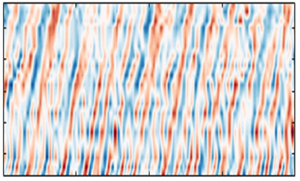
Figure 7 shows a subset of the instantaneous structure of the wall pressure along the tail. Here, contours of the pressure normalized on the  $p_{rms}$ of the original signal are shown, with the vertical axis representing the location on the tail, and the horizontal axis representing a 0.2 second subset from a full 32 seconds. These contours are characterized by forward-leaning ridges that appear to alternate in sign, with positive ridges (red) often succeeded by negative ones (blue). The forward inclination of the structure is consistent with the expected downstream convection of the pressure-producing motions with time. This is particularly interesting and unexpected, with the convective features appearing to be quasi-periodic and occasionally strong, and tending to remain coherent over long distance, approximately ${\rm \Delta} x \sim 0.55D$ or 9 $\delta$.

Figure 7. Snapshot of the instantaneous pressure along the BOR tail, with time on the horizontal axis, and streamwise position on the vertical axis. Coloured contours show the pressure normalized with corresponding root-mean-square values. This snapshot corresponds to a 0.2 second subset from a total of 32 seconds.
Investigating these unexpected quasi-periodic ridges and their relation to the overriding flow could provide fundamental insight into the broadband success of the wall-wake scaling ( $\tau _w,U_e, \delta$) on the pressure spectrum. Below, we explore this feature through a conditional averaging scheme, beginning with an outline of the procedure and followed by a discussion of the resulting structure and its characteristics, such as the scaling, convection velocity, and differences with a ZPG layer. Finally, we attempt to relate this feature to the structure of the overriding flow.
Noting that the quasi-periodic ridges have a high amplitude with  $p' > p_{rms}$, we consider a conditional averaging scheme based on peak detection in the instantaneous time series. Figure 8 shows the low-pass filtered pressure signal at $x/D = 2.85$ for the same 0.2 second interval shown in figure 7, filtered at 4000 Hz (consistent with spectral analysis) through an infinite impulse response filter. To extract the high-amplitude events, we prescribe a qualifying threshold $\varGamma = k p_{rms}$ and identify every peak stronger than the threshold $\varGamma$ as an event, as shown with the blue triangles in figure 8 using $k = 2$. The start time $t_o^i$ for each event is documented, and the original pressure signal $p(t)$ is centred about $t_o^i$, resulting in a conditional time series $p_i(t-t_o^i)$. This process is repeated for all $N$ identified events, and ensemble averaged to yield the conditional structure
 \begin{equation} \langle p_c(t-t_o)\rangle = \frac{1}{N} \sum_{i=1}^{N} p_i(t-t_o^i). \end{equation}
Figure 8. Snapshot of the pressure signal at  $x/D$=2.85 corresponding to the time interval shown in figure 7. The blue dashed line represents the threshold $\varGamma$ used for identifying the conditional events corresponding to quasi-periodic pressure features. Inverted triangles show the identified high-amplitude pressure peaks.
It must be noted that the choice of threshold,  $\varGamma = k p_{rms}$, should be high enough to distinguish a significant event from the general background, while being simultaneously low enough that it is identified a sufficient number of times to ensure statistical convergence. From a quick study, we determined that $k = 2$ satisfied this requirement with no appreciable difference in the end result for $k \in [1.2, 3]$. The resulting pattern, for both negative and positive pressure peaks, was independent of the threshold, with peak amplitude $|1.7\varGamma |$. We also found that the number of identified events decreased exponentially with threshold, and for $k = 2$, approximately 2000 events were identified, corresponding to a frequency of 0.1 % and contributing to approximately 12 % of the ensemble root-mean-square pressure.
The resulting conditional structure is shown in figure 9(a) for  $x/D=2.85$, along with the uncertainty bounds based on a 95 % confidence interval. The structure comprises a decaying peak with a negative overshoot that is symmetric in time, consistent with a time-reversal symmetry expected from a convective process. In fact, we observed such structures at all measured locations on the BOR tail, shown in figure 9(b), with pressure normalized by $\tau _w$, and time delay by $\delta /U_e$ on the horizontal axis. The non-dimensional pressure structure appears to have a similar form along the BOR tail, with a characteristic peak at 13–17 $\tau _w$ and time scale approximately 4 $\delta /U_e$. This is consistent with the broadband success of wall-wake scaling ( $\tau _w, U_e, \delta$) that we observed in the wall-pressure spectrum shown in figure 5. To further investigate the convective properties and to verify if the conditional structure represents the quasi-periodic ridges seen in the instantaneous maps earlier (figure 7), one can examine the pressure signals upstream and downstream of a specified anchor position (say $x/D = 2.85$), and conditionally average the time series based on the events detected at the anchor position:
 \begin{equation} \langle p_c(\xi,t-t_o)\rangle = \frac{1}{N} \sum_{i=1}^{N} p_i(\xi,t-t_o^i), \end{equation}
where  $\xi$ represents the separation ( $x - x'$) of a microphone at $x$ from the anchor at $x'$. If the structure is convective, then it should be recovered at other streamwise positions, albeit shifted in time.

Figure 9. (a) The conditional structure of the wall pressure at  $x/D = 2.85$, with the error bounds (cyan) based on a 95 % confidence interval. (b) Conditional structure from all streamwise stations, with the pressure normalized on the local wall shear stress $\tau _w (x)$, and the time delay normalized with the outer time scale $\delta /U_e$ (x). See figure 4 for legend.
The conditionally averaged structure at all streamwise positions, based on the events detected at the anchor position  $x/D = 2.85$, is shown in figure 10. Contours of the conditional pressure are shown as a function of the non-dimensional time delay on the horizontal axis, and spatial separation on the vertical axis. While the horizontal slice at $\xi /\delta = 0$ (zero streamwise separation) corresponds to the structure shown in figure 9 with a peak (red) at zero time delay accompanied by negative overshoots (blue), the horizontal slices along other separations show a similar signature but shifted in time. In fact, the central, forward-leaning ridge in the conditional structure, along with the weak but periodic patterns to the left and right, shows that the identified conditional structure is persistent along the tail boundary layer, convecting downstream. Considering that these quasi-periodic ridges appear in the instantaneous flow, detected quantitatively through the conditional scheme described above, which appear to scale along the tail with wall-wake scaling, this could explain the broadband collapse of the wall-pressure spectra scaled with the wall-wake scaling.

Figure 10. Space–time characteristics of the conditional structure obtained by conditionally averaging the pressure signals at upstream and downstream locations based on events detected at  $x/D = 2.85$. The horizontal axis shows the normalized time delay, and the vertical axis shows the normalized streamwise separation, while contour levels represent the conditionally averaged pressure in pascals.
In fact, this feature is also reflected in the ensemble-averaged space–time correlations shown in figures 11(a–c), obtained without any conditioning, defined as
 \begin{equation} R_{pp} \equiv E[p(x,t)\,p(x+\xi,t+\tau)], \end{equation}
where  $\xi$ is the longitudinal separation along the tail, and $\tau$ corresponds to the time delay. Results are shown for representative stations along the tail, with $x/D$ values 2.73, 2.85, 3.05, in figures 11(a–c), respectively. Furthermore, in each case, the correlation is normalized by the corresponding mean-square value, resulting in a maximum of 1 that corresponds to the autocorrelation ( $\xi = \tau = 0$). Such maps are generally characterized by a narrow diagonal band along which most of the energy is concentrated. This is often referred to as the convective ridge; it implies that the pressure-producing motions, despite evolving, remain correlated as they convect downstream with time. In addition to the convective ridge observed in ZPG turbulent boundary layer flows (Choi & Moin Reference Choi and Moin1990), we observe negative off-diagonal bands with peak level $-$0.4. This is consistent with the conditional pressure pattern observed earlier. Furthermore, at zero spatial separation, i.e along the horizontal line corresponding to $\xi /\delta =0$, the time delay corresponding to a decayed correlation is close to the time scale of the conditional structure discussed above.

Figure 11. Space–time correlation function of the wall pressure shown at representative locations on the tail; see (3.4) for definition. Here, (a)  $x/D = 2.73$, (b) $x/D = 2.85$, and (c) $x/D = 3.05$.
Assuming that the pressure-producing motions are convecting at the local mean velocity, we can ascertain their tentative location if we know the convection velocity of the quasi-periodic feature. A rudimentary estimate based on the slope of the forward-leaning ridges seen in the instantaneous structure (figure 7) is approximately 0.6 $U_e$, which corresponds to the outer regions in the layer, specifically, the location of the inflection point in the mean velocity profiles. However, to confirm quantitatively the preliminary estimate, we consider the convection velocity based on the slope of the ridge in the conditional space–time pattern (figure 10). The convection velocity at each separation is estimated from the slope of the peak as
 \begin{equation} U_{c}(\xi_) = \frac{\xi}{\tau_{peak}(\xi)}, \end{equation}
where  $U_{c}(\xi )$ represents the convection velocity corresponding to a separation $\xi = |x - x'|$, and $\tau _{peak}$ is the time delay corresponding to the peak location for $\xi$. The resulting convection velocity of the quasi-periodic feature is shown in figure 12, along with the convection velocity estimated from the ensemble-averaged cross-correlations (figure 11), for all anchor microphones using (3.5). While the vertical axis represents the convection velocity $U_{c}$ normalized with the edge velocity at the anchor microphone $U_e'$, the horizontal axis represents the spatial separation $\xi$ normalized on $\delta$ . The trends from the conditional structure are consistent with the ensemble-averaged estimates: the convection velocity increases with separation and asymptotes to approximately 0.6 $U_e$ for $\xi /\delta > 2$. For smaller separations, one would expect the small-scale turbulence occurring near the wall to dominate the correlations, resulting in a lower convection velocity consistent with the lower mean speeds near the wall. However, these small-scale fluctuations appear to decorrelate at larger separations, such that the large-scale motions dominate the correlation, and are centred away from the wall and convect at relatively faster speeds. This 0.6 $U_e$ asymptote is consistent with the rudimentary estimate from figure 7, suggesting that the motions with quasi-periodic pressure footprints are centred at the inflection point in the outer region of the mean velocity profiles, where the mean velocity is $0.594 U_e \pm 0.052 U_e$ (see figure 15 in BHAD).

Figure 12. Convection velocity of the wall pressure shown as a function of spatial separation between the probes, normalized on the boundary layer thickness. Each curve corresponds to an anchor microphone position, with the corresponding colour and symbols shown in the legend. Black squares show the convection velocity of the conditional pressure pattern from figure 10.
The existence of these quasi-periodic motions that track the inflection point provides evidence in favour of the ESL hypothesis for strong APG boundary layers. Furthermore, it is clear that the shear-layer motions play a significant role in the near-wall turbulence and on the wall pressure, supporting the broadband success of the wall-wake scaling ( $\tau _w,U_e, \delta$) on the wall-pressure spectrum. However, if the outer-layer motions are such significant sources for the wall pressure, then one would expect an outer-region scale – such as the maximum shear stress or the dynamic pressure – to dictate the wall-pressure amplitude, instead of $\tau _w$ as observed. One likely explanation stems from a scenario where the large-scale shear-layer motions are superposed on the underlying boundary layer turbulence with its associated near-wall cycle. In this case, the shear-layer motions would drive the wall-pressure dynamics not by directly slapping the wall but instead by playing a strong but indirect role through modulation of the near-wall boundary layer turbulence and therefore influencing both the skin friction and wall pressure. Further investigation into these aspects can be performed by rigorous examination of the source terms in the pressure Poisson equation, including the pressure-gradient terms in the mean-shear terms, in addition to the nonlinear terms. An alternative and simpler approach is to examine the contribution of the shear-layer motions to the wall-pressure spectrum analytically, with a mathematical model that captures the essential features of the convecting roller eddies, similar to the work of Dhanak, Dowling & Si (Reference Dhanak, Dowling and Si1997) on the contribution of hairpin vortices.
4. Conclusions
This work presents the wall pressure signature of an axisymmetric boundary layer under a strong adverse pressure gradient (APG). Measurements were made on the tail of a body of revolution with a longitudinal array of surface-mounted microphones, documenting the fluctuating pressure imposed by a sharply decelerating non-equilibrium boundary layer. The wall-pressure spectrum and its scaling are discussed along with the space–time structure to reveal the combined effects of APG and lateral curvature.
As the flow decelerates downstream, the mean-square pressure drops together with the wall shear stress ( $\tau _w$), and is consistently approximately 7 $\tau _w$. The associated dimensional spectrum weakened significantly, with a broadband reduction of over 15 dB per Hz. Much of this variation seems to be tracked by the wall-wake scaling, where $\tau _w$ is the pressure scale, and $\delta /U_e$ is the time scale. Here, $\delta$ is the boundary layer thickness, and $U_e$ is the edge velocity. However, considering that this study is focused on a single configuration, additional work is needed to characterize the parameter range for the validity of the wall-wake scaling in strong APG boundary layers.
The reasons for broadband success of the wall-wake scaling, even in the viscous  $f^{-5}$ regions, were examined by considering the space–time structure of the wall pressure. Preliminary examination of the instantaneous fluctuations revealed the presence of a quasi-periodic feature that appeared to remain correlated over a measured longitudinal extent, which was over $9\delta$. Detailed analysis through peak detection revealed a conditional structure with a strongly coupled negative trough followed by a positive peak, which is indicative of a convective roller. Also, the amplitude and time scale of this feature appeared to scale with $\tau _w$ and $\delta /U_e$, which is reminiscent of the success of wall-wake scaling on the pressure spectrum.
Furthermore, these features were observed to travel downstream at speeds matching those at the inflection point in the mean velocity profile (and the outer turbulence stress peak), providing evidence to the embedded shear layer hypothesis for strong APG flows. However, the success of  $\tau _w$ despite the evident role of the outer-layer motions is discussed with reference to a scenario where the large-scale embedded layer turbulence is superposed on the underlying near-wall boundary layer turbulence. It is hypothesized that the shear-layer motions play a strong but indirect role by modulating the near-wall turbulence and consequently the wall friction and pressure. Suggestions are made for further investigation to evaluate this hypothesis.
Acknowledgements
The authors acknowledge the contributions of Dr C. Hickling and Mr A. Millican with CAD and wind tunnel testing. The authors would like to thank Dr D. Zhou at Cal Tech and Dr M. Wang at the University of Notre Dame for sharing their large eddy simulation data. We also thank Drs S. Glegg, W. Blake and J. Anderson for helpful discussions and advice on the project. Finally, we would like to thank the reviewers for helpful suggestions, particularly with conditional analysis in § 3.3.
Funding
This research was sponsored by the Office of Naval Research through grants N00014-17-1-2698 and N00014-20-1-2650, with Drs K.-H. Kim, J. Muench and J. Young as programme managers.
Data availability statement
The dataset for fluctuating wall pressure is available at https://doi.org/10.7294/22264045
Declaration of interests
The authors report no conflict of interest.
Appendix. On using friction velocity from large eddy simulation
Since friction velocity is a critical parameter associated with wall pressure, and since we do not have either direct measurements or any established hypothesis for APG flows, we rely on Reynolds-number-matched wall-resolved LES over the BOR (Zhou et al. Reference Zhou, Wang and Wang2020). While this seems to be a bold manoeuvre, detailed comparisons of the pressure and velocity statistics provide encouraging support. First, comparisons of the mean surface pressure (presented in figure 7 of the companion paper BHAD), mean velocity profiles, turbulence statistics and spectra (in Zhou et al. Reference Zhou, Wang and Wang2020) suggest that the LES flow is dynamically similar to the experimentally realized flow. More significant are the comparisons of fluctuating wall-pressure spectrum shown in figure 13. Shown for various representative locations along the BOR tail, the autospectra from experiment and LES generally agree to within 3 dB and to within 1 dB in the high-frequency regions ( $\,fD/U_\infty >10$), which are governed by the near-wall skin-friction-generating motions. Indeed, we also observed that the viscous scaling (with $f\nu /{u_\tau ^2}$ and $\tau _w$ as the pressure scale) collapsed the viscous roll-off regions from all the streamwise locations to within 2 dB (figure 6a), which otherwise showed a variation of approximately 20 dB (figure 4). This suggests that for the purposes of understanding the scaling behaviour and analysis presented in this paper, the skin friction from LES is reliable. Of course, one must exercise caution when extending this to a rigorous analysis, which requires accurate estimates of skin friction in cases such as when generating training data sets and validating wavenumber–frequency spectrum models.

Figure 13. Comparison of the wall pressure spectra between experiments (solid lines) and LES (dashed lines) at representative locations on the BOR. Red shows  $x/D = 2.85$, purple shows $x/D = 2.76$, and pink shows $x/D = 3.02$ (see full legend in figure 4).


 Open access