


1 Introduction
Thorough understanding of the turbulent atmospheric boundary layer (ABL) is required for a wide variety of applications including numerical weather prediction, pollutant transport and wind energy. The ABL has been studied numerically extensively since Deardorff (Reference Deardorff1972) under varying regimes of stratification using large eddy simulation (LES). In the limit of neutral atmospheric stratification, the flow is statistically quasi-stationary and reduces to the turbulent Ekman layer (Deardorff Reference Deardorff1970). The Ekman layer flow, which is a balance of Coriolis, pressure gradient and surface drag forces, also presents in the oceanic surface layer (Iooss, Nielsen & True Reference Iooss, Nielsen and True1978; Spooner Reference Spooner1983). When projected into an Earth-fixed domain of interest, Earth’s rotation acts as vertical and horizontal components, as shown in figure 1(a). Leibovich & Lele (Reference Leibovich and Lele1985) noted that the Ekman layer instability is sensitive to the direction of the geostrophic wind as a result of the horizontal component of Earth’s rotation at finite Rossby numbers. However, the overwhelming majority of numerical ABL studies has neglected this component (see e.g. Moeng (Reference Moeng1984)). Coleman, Ferziger & Spalart (Reference Coleman, Ferziger and Spalart1990) showed using direct numerical simulation at low Reynolds numbers, both the friction velocity ( $u^{\ast }=\sqrt{\unicode[STIX]{x1D70F}_{w}/\unicode[STIX]{x1D70C}}$, where $\unicode[STIX]{x1D70F}_{w}$ is the surface shear stress and $\unicode[STIX]{x1D70C}$ is density) and the relative misalignment between the pressure gradient and the surface shear stress are strongly sensitive to the direction of geostrophic velocity at non-polar latitudes. Zikanov, Slinn & Dhanak (Reference Zikanov, Slinn and Dhanak2003) revealed the sensitivity of the unstratified neutral ABL with an infinite Reynolds number to the horizontal component of Earth’s rotation. While the horizontal component of Earth’s rotation does not appear in the Reynolds-averaged horizontally homogeneous ABL momentum equations, its role persists through non-hydrostatic and transient effects (Leibovich & Lele Reference Leibovich and Lele1985). More recent studies of the moderate Reynolds number turbulent Ekman layer have continued to neglect the horizontal component of Earth’s rotation (see e.g. Momen & Bou-Zeid (Reference Momen and Bou-Zeid2017) and Gohari & Sarkar (Reference Gohari and Sarkar2018)). Meanwhile, neglecting the horizontal component of Earth’s rotation has been shown to be invalid in oceanic flows (Gerkema & Shrira Reference Gerkema and Shrira2005; Gerkema et al. Reference Gerkema, Zimmerman, Maas and Van Haren2008; Grisouard & Thomas Reference Grisouard and Thomas2015; Delorme & Thomas Reference Delorme and Thomas2019).
As shown in scaling analysis by Wyngaard (Reference Wyngaard2010), the Coriolis term in the equation of motion in the atmosphere is relevant when  $u^{2}/L\sim \unicode[STIX]{x1D6FA}u$, where $u$ is a relevant velocity scale, $L$ is a length scale and $\unicode[STIX]{x1D6FA}$ is the rotational rate of the Earth. The vertical and horizontal components of Earth’s rotation are governed through the same scaling laws. The horizontal component of Earth’s rotation cannot be neglected through scaling analysis if the vertical component is relevant to the equations of motion. However, the horizontal scales of motion are considerably larger than the vertical in the ABL (resulting in low vertical speeds compared to horizontal speeds (see e.g. Stull (Reference Stull2012))), and therefore the role of the horizontal component of Earth’s rotation in the horizontal momentum balance may be expected to be marginal. However, the horizontal component not only influences the vertical balance of momentum but also acts indirectly in the horizontal momentum balance through the Reynolds stress terms (Coleman et al. Reference Coleman, Ferziger and Spalart1990).
The simplified Ekman layer problem is dissimilar from the character of field measurements of the turbulent ABL (Price & Sundermeyer Reference Price and Sundermeyer1999); this difference principally manifests as a result of buoyancy and density stratification. While numerical simulations of the more realistic stable ABL with buoyancy have been performed (see e.g. Mason & Derbyshire (Reference Mason and Derbyshire1990)), they generally neglect the horizontal component of Earth’s rotation. To the authors’ knowledge, no study has provided a quantitative justification for neglecting the horizontal component in high Reynolds number flows with buoyancy and density stratification effects. A goal of this study is to develop a quantitative description of when this simplifying assumption is valid or invalid in fundamental ABL flows.
Beyond simplified homogeneous ABL flows, roughness elements such as wind turbines introduce significant heterogeneity and enhanced turbulence (see e.g. Meneveau (Reference Meneveau2019)). When wind turbines are placed in close proximity in wind farms, the cumulative momentum deficit significantly impacts the ABL equilibrium state by inducing a developing internal boundary layer (Chamorro & Porte-Agel Reference Chamorro and Porte-Agel2011; Meneveau Reference Meneveau2012) as well as a large-scale wind farm wake (Nygaard & Newcombe Reference Nygaard and Newcombe2018) resulting in the enhancement of the natural turbulent ABL vertical transport of kinetic energy. Individual wind turbines create wakes which have a streamwise length scale which is an order or magnitude larger than the turbine diameter (Chamorro & Porté-Agel Reference Chamorro and Porté-Agel2009); Platis et al. (Reference Platis, Siedersleben, Bange, Lampert, Bärfuss, Hankers, Cañadillas, Foreman, Schulz-Stellenfleth and Djath2018) have reported wind farm wakes of the order of tens of kilometres in length. Since Coriolis forces influence flow structures on large length scales and affect vertical transport, a thorough understanding of their impact has become increasingly important in the design and operation of large wind farms (Abkar & Porté-Agel Reference Abkar and Porté-Agel2016; van der Laan & Sørensen Reference van der Laan and Sørensen2017; Eriksson et al. Reference Eriksson, Breton, Nilsson and Ivanell2019; Gadde & Stevens Reference Gadde and Stevens2019). All previous studies of the influence of Coriolis forces in wind farm simulations have neglected the horizontal component of Earth’s rotation and the sensitivity of phenomena such as the vertical entrainment of kinetic energy above large wind farms to the direction of the geostrophic velocity have not been examined (see e.g. Lu & Porté-Agel (Reference Lu and Porté-Agel2011), Archer, Mirzaeisefat & Lee (Reference Archer, Mirzaeisefat and Lee2013) and Allaerts & Meyers (Reference Allaerts and Meyers2015)). It is important to understand the role of the horizontal component of Earth’s rotation in the interaction between wind turbine arrays and the ABL since this interaction dictates the optimal design and operation of wind farms (Stevens et al. Reference Stevens, Hobbs, Ramos and Meneveau2017; Allaerts & Meyers Reference Allaerts and Meyers2018).
In § 2 the influence of the direction of the geostrophic velocity is examined in LES of a model wind farm within the conventionally neutral ABL. The resulting sensitivity is examined through an analysis of the mean kinetic energy (MKE), turbulence kinetic energy (TKE) and Reynolds stress budgets as well as the turbulence structure including sweeps and ejections, two-point correlations and integral length scales. The sensitivity is also examined in a statically stable ABL and comments on transient stability transitions are made. In § 3, the sensitivity to the direction of the geostrophic velocity is examined as a function of the spacing of turbines within the model wind farm. A model for the influence of the geostrophic velocity direction on the vertical transport in the ABL is also proposed. Conclusions are made in § 4.
2 Influence of geostrophic direction on the wind farm ABL
2.1 Conventionally neutral ABL without drag disks numerical set-up
The present study focuses on the LES of the ABL with the inclusion of a model wind farm represented as drag disk elements. The filtered, incompressible, infinite Reynolds number LES equation for momentum (under the high Reynolds number limit) is
 $$\begin{eqnarray}\frac{\unicode[STIX]{x2202}u_{i}}{\unicode[STIX]{x2202}t}+u_{j}\frac{\unicode[STIX]{x2202}u_{i}}{\unicode[STIX]{x2202}x_{j}}=-\frac{\unicode[STIX]{x2202}p}{\unicode[STIX]{x2202}x_{i}}-\frac{\unicode[STIX]{x2202}\unicode[STIX]{x1D70F}_{ij}}{\unicode[STIX]{x2202}x_{j}}+f_{i}+\frac{\unicode[STIX]{x1D6FF}_{i3}}{Fr^{2}}(\unicode[STIX]{x1D703}-\unicode[STIX]{x1D703}_{0})-\frac{2}{Ro}\unicode[STIX]{x1D700}_{ijk}\unicode[STIX]{x1D6FA}_{j}u_{k}-\frac{\unicode[STIX]{x2202}P^{G}}{\unicode[STIX]{x2202}x_{i}},\end{eqnarray}$$
 where  $u_{i}$ is the velocity in the $x_{i}$ direction, $t$ is time, $P^{G}$ is the non-dimensional geostrophic pressure (assumed to have a linear spatial variation within the simulated domain) and $\unicode[STIX]{x1D6FF}$ is the Kronecker delta. The non-dimensional pressure is given as $p$,
$p$,  $\unicode[STIX]{x1D70F}_{ij}$ is the subfilter-scale stress tensor (only the deviatoric components of the stress tensor are modelled), $\unicode[STIX]{x1D703}$ is the non-dimensional potential temperature, $\unicode[STIX]{x1D703}_{0}$ is the reference non-dimensional potential temperature and $G$ is the geostrophic velocity (value of $u$ as $z\rightarrow \infty$). The drag disk wind turbine model forcing is given by $f_{i}$. The Froude number is $Fr=G/\sqrt{gL}$ where $g$ is the gravitational acceleration and $L$ is the dimensional length scale. The $x$-axis corresponds to the easting (west to east axis) direction and the $y$-axis corresponds to the northing (south to north axis) direction. All velocities will be non-dimensionalized by the geostrophic velocity magnitude, although similar observations can be made if the friction velocity is selected for normalization (see appendix A). The Coriolis forces are governed by the non-dimensional Rossby number $Ro=G/\unicode[STIX]{x1D714}L$ where $\unicode[STIX]{x1D714}$ is Earth’s rotational rate. The rotation vector at a latitude, $\unicode[STIX]{x1D719}$, can be written as $\unicode[STIX]{x1D6FA}_{E}=[0,\unicode[STIX]{x1D714}\cos (\unicode[STIX]{x1D719}),\unicode[STIX]{x1D714}\sin (\unicode[STIX]{x1D719})]$, and $\unicode[STIX]{x1D6FA}=\unicode[STIX]{x1D6FA}_{E}/\unicode[STIX]{x1D714}$. Neglecting the horizontal component of Earth’s rotation (often called the traditional approximation in geophysical flows) results in $\unicode[STIX]{x1D6FA}_{2}=0$. Since all Coriolis terms are governed by the same Rossby number and latitude, it is important to note that should scaling analysis conclude that $\unicode[STIX]{x1D6FA}_{3}$ is a relevant in the flow, $\unicode[STIX]{x1D6FA}_{2}$ cannot be neglected through scaling. Since the flow is not hydrostatic, the Coriolis term $2\unicode[STIX]{x1D6FA}_{2}u_{1}/Ro$ which appears in the $u_{3}$ momentum equation should not be neglected since it is not negligible compared to gravity and pressure.
Equation (2.1) is solved numerically by expressing the geostrophic pressure gradient in terms of the geostrophic velocity,  $G$ as
 $$\begin{eqnarray}\frac{\unicode[STIX]{x2202}P^{G}}{\unicode[STIX]{x2202}x_{i}}=-\frac{2}{Ro}\unicode[STIX]{x1D700}_{ijk}\unicode[STIX]{x1D6FA}_{j}G_{k}.\end{eqnarray}$$
In the wall-normal direction, the right-hand side of (2.1) is expressed as
 $$\begin{eqnarray}\displaystyle & & \displaystyle \displaystyle \left[-\frac{\unicode[STIX]{x2202}p}{\unicode[STIX]{x2202}x_{3}}+\frac{1}{Fr^{2}}(\overline{\unicode[STIX]{x1D703}}-\unicode[STIX]{x1D703}_{0})+\frac{2}{Ro}(G_{2}-\overline{u_{2}})\unicode[STIX]{x1D6FA}_{1}-\frac{2}{Ro}(G_{1}-\overline{u_{1}})\unicode[STIX]{x1D6FA}_{2}\right]\nonumber\\ \displaystyle & & \displaystyle \quad +\displaystyle \frac{1}{Fr^{2}}(\unicode[STIX]{x1D703}-\overline{\unicode[STIX]{x1D703}})+\frac{2}{Ro}([u_{1}-\overline{u}_{1}]\unicode[STIX]{x1D6FA}_{2}-[u_{2}-\overline{u}_{2}]\unicode[STIX]{x1D6FA}_{1})+f_{3}-\frac{\unicode[STIX]{x2202}\unicode[STIX]{x1D70F}_{3j}}{\unicode[STIX]{x2202}x_{j}},\end{eqnarray}$$
 where  $\overline{\cdot }$ denotes horizontal ( $x_{1}{-}x_{2}$ plane) averaging. The bracketed terms in (2.3) are interpreted as a pseudo-pressure $p^{\ast }$
 $$\begin{eqnarray}-\frac{\unicode[STIX]{x2202}p^{\ast }}{\unicode[STIX]{x2202}x_{3}}=-\frac{\unicode[STIX]{x2202}p}{\unicode[STIX]{x2202}x_{3}}+\underbrace{\frac{1}{Fr^{2}}(\overline{\unicode[STIX]{x1D703}}-\unicode[STIX]{x1D703}_{0})+\frac{2}{Ro}(G_{2}-\overline{u_{2}})\unicode[STIX]{x1D6FA}_{1}-\frac{2}{Ro}(G_{1}-\overline{u_{1}})\unicode[STIX]{x1D6FA}_{2}}_{No\,dependence\,on\,x_{1}\,and\,x_{2}}.\end{eqnarray}$$
 This manipulation of the pressure allows for the use of spectral numerics in the  $x_{1}$ and $x_{2}$ directions using well-posed boundary conditions for the pseudo-pressure $p^{\ast }$ to discretely satisfy the continuity constraint ( $\unicode[STIX]{x2202}u_{j}/\unicode[STIX]{x2202}x_{j}=0$). Note that this manipulation involving $p^{\ast }$ is mathematically equivalent to solving for the non-hydrostatic dynamics in (2.1) under a purely horizontal geostrophic pressure gradient.
The filtered equation for the non-dimensional potential temperature is
 $$\begin{eqnarray}\frac{\unicode[STIX]{x2202}\unicode[STIX]{x1D703}}{\unicode[STIX]{x2202}t}+u_{j}\frac{\unicode[STIX]{x2202}\unicode[STIX]{x1D703}}{\unicode[STIX]{x2202}x_{j}}=-\frac{\unicode[STIX]{x2202}q_{j}^{SGS}}{\unicode[STIX]{x2202}x_{j}},\end{eqnarray}$$
 where  $\unicode[STIX]{x1D703}$ is the filtered non-dimensional potential temperature and $q_{j}^{SGS}$ is the subgrid-scale (SGS) heat flux. The momentum and active scalar potential temperature equations are coupled with the Froude number as the governing parameter.
(a) Sketch of the projection of Earth’s rotation into a west to east computational domain. Sketches of the computational domains for the (b) west to east and (c) east to west geostrophic flows. The cardinal directions are shown in index notation. The computational domain is shown in  $(x,y,z)$. The mean velocity at the wind turbine model hub height is $\overline{u}(z_{h})$ and the angle between $\overline{u}(z_{h})$ and the geostrophic velocity vector is $\unicode[STIX]{x1D6FC}$. The mean wind direction as a function of height $u(z)$ is shown in orange.

The ABL LES simulations are performed using an incompressible (Boussinesq) flow code PadéOps (https://github.com/FPAL-Stanford-University/PadeOps) (Ghate & Lele Reference Ghate and Lele2017). The solver uses Fourier collocation in the horizontally homogeneous directions and a sixth-order staggered compact finite difference scheme in the vertical direction (Nagarajan, Lele & Ferziger Reference Nagarajan, Lele and Ferziger2003). Temporal integration is performed using a fourth-order strong stability preserving (SSP) variant of a Runge–Kutta scheme (Gottlieb, Ketcheson & Shu Reference Gottlieb, Ketcheson and Shu2011). Ekman transport is neglected due to the horizontal homogeneity (Zikanov et al. Reference Zikanov, Slinn and Dhanak2003). Subgrid-scale closure is specified using the sigma subfilter-scale model (Nicoud et al. Reference Nicoud, Toda, Cabrit, Bose and Lee2011); the scalar diffusivity is modelled using a Prandtl number of  $Pr=0.4$ (validated in Ghate & Lele Reference Ghate and Lele2017, for a stably stratified atmospheric boundary layer flow). All results presented in this paper correspond to rough wall boundary layers with a roughness length scale of 10 cm, and are assumed to be periodic in the two horizontal directions ( $x$ and $y$) with a domain size of $6.4\times 3.2\times 2.4~\text{km}$. The wall model is constructed using Monin–Obukhov similarity theory (Moeng Reference Moeng1984). The simulations are initialized with a uniform potential temperature up to a height of 700 m (with superposed random noise perturbations) above which there is a statically stable potential temperature inversion of $3~\text{K}~\text{km}^{-1}$. Rayleigh damping is enforced within the top $25\,\%$ of the simulated domain. The influence of the vertical domain height and the Rayleigh damping are tested in appendix A. The simulation has $512$, $256$ and $384$ grid points in the $x$,
$x$,  $y$ and $z$ directions respectively. The domain is discretized using a uniform mesh. Simulations with varying resolutions were performed to establish grid independence of the results discussed in this paper. The grid independence of the drag disk model simulations are discussed in § 2.4. A latitude of $\unicode[STIX]{x1D719}=45^{\circ }$ is selected for simplicity, and the implied Rossby number based on the initial boundary layer height is $98$. The Froude number based on the initial boundary layer height is $0.06$. A precursor simulation without wind turbine models is run until convergence to the statistically quasi-stationary state. Comments on the quasi-steady state are discussed in appendix A.
Conventionally neutral ABL without drag disk models time and horizontally averaged (a) velocity, (b) Reynolds stresses, (c) wind direction and (d) wind speed. (a–c) Solid lines indicate west to east geostrophic wind and dashed lines indicate east to west geostrophic wind. The dashed-dotted lines neglect the horizontal component of Earth’s rotation by setting  $\unicode[STIX]{x1D6FA}_{y}=0$; (d) (blue ●) west to east geostrophic wind and (blue ▴) east to west geostrophic wind.

2.2 Conventionally neutral ABL without drag disk results
Simulations are performed with the geostrophic velocity directed west to east and east to west. Sketches of the computational domains within the cardinal direction coordinate system can be seen in figure 1(b,c). Since the  $x$-axis of the computational domain is aligned with the geostrophic velocity vector, the projection of $\unicode[STIX]{x1D6FA}_{2}$ into the computational domain, referred to hereafter as $\unicode[STIX]{x1D6FA}_{y}$, will maintain the same magnitude but flip in sign between the two cases. When Earth’s rotational vector is projected into the computational domain with an arbitrary rotation, it is given by $\unicode[STIX]{x1D6FA}=[\cos (\unicode[STIX]{x1D719})\sin (\unicode[STIX]{x1D703}),\cos (\unicode[STIX]{x1D719})\cos (\unicode[STIX]{x1D703}),\sin (\unicode[STIX]{x1D719})]$ where $\unicode[STIX]{x1D703}$ is the angle measured between the domain $x$-axis and the easting axis. As a result of the domain rotation, the geostrophic velocity direction is misaligned with the easting axis by $\unicode[STIX]{x1D703}$. In the west to east geostrophic velocity case $\unicode[STIX]{x1D703}=0^{\circ }$ and in the east to west case $\unicode[STIX]{x1D703}=180^{\circ }$. The comparison between these two conventionally neutral ABL simulations without wind turbines is shown in figure 2. The mean velocity profiles are slightly different between the two cases. The friction velocities are $0.231\pm 0.0009$ and $0.245\pm 0.0025~\text{m}~\text{s}^{-1}$ in the west to east and east to west geostrophic direction cases respectively, representing a $6\,\%$ difference. The errors represent the standard deviation in horizontally averaged $u^{\ast }$ as a function of time. The friction velocities for the two simulations during the time-averaging window are shown in appendix A. Inertial oscillations result in fluctuations of $u^{\ast }$ about the quasi-steady mean value. However, the friction velocities of the west to east simulation have a persistent offset from the friction velocities of the east to west simulation in the inertial oscillations.
These differences are consistent with the direct numerical simulation of Coleman et al. (Reference Coleman, Ferziger and Spalart1990) at low Reynolds numbers. The magnitudes of  $u^{\ast }$ are representative of offshore ABLs (Allaerts & Meyers Reference Allaerts and Meyers2015). The difference in surface stress also manifests as a difference in the Reynolds stresses associated with the vertical transport of kinetic energy. Figure 2(b) shows $\overline{u^{\prime }w^{\prime }}$ for the two cases. While the peak $\overline{u^{\prime }w^{\prime }}$ location is the same in the two simulations, the peak magnitudes are $12\,\%$ different. Since the vertical transport and mean momentum balance appear to be sensitive to the geostrophic direction, we can conclude that neglecting the horizontal component of Earth’s rotation is inapplicable in the present high Reynolds number conventionally neutral ABL case. The veer profiles are also a function of the geostrophic wind direction, as shown in figure 2(c). The logarithmic speed profiles are shown in figure 2(d) where there is no significant sensitivity in the log law due to the difference in geostrophic direction other than the shift due to the change in the friction velocity.
The influence of neglecting the horizontal component of Earth’s rotation is directly tested by setting  $\unicode[STIX]{x1D6FA}_{y}=0$ explicitly in the conventionally neutral ABL without drag disks. With $\unicode[STIX]{x1D6FA}_{y}=0$, the simulation is invariant to the geostrophic wind direction. The results of this simulation are also included in figure 2. The influence of neglecting the horizontal component is similar to the influence of the geostrophic wind direction, although less pronounced. It is expected that the differences between the west to east and east to west geostrophic wind cases will be larger than the differences between the west to east and the $\unicode[STIX]{x1D6FA}_{y}=0$ case. While in the cases of changing geostrophic wind direction, the Reynolds stress Coriolis source/sink term will reverse sign while maintaining a similar magnitude; with $\unicode[STIX]{x1D6FA}_{y}=0$, the Coriolis source/sink will reduce in magnitude. The rationale for this result will be more thoroughly explained in the following sections through Reynolds stress budget analysis (§ 2.4).
2.3 Conventionally neutral ABL with drag disk numerical set-up
From the statistically quasi-stationary conventionally neutral ABL simulations, a model wind farm is introduced into the simulation. There are 36 wind turbines in the domain corresponding to spacing of  $8.5D$ and $4.2D$ in the easting and northing directions respectively where $D$ is the turbine diameter. The actuator disk model is used to represent the model turbines (Calaf, Meneveau & Meyers Reference Calaf, Meneveau and Meyers2010) which have a diameter of 126 m and a hub height of 100 m. The coefficient of thrust for each turbine is $0.75$. The turbine spacing is uniform in the domain. The wind turbine model drag disks are aligned with the $x$-axis in the computational domain.
With the inclusion of the wind turbine models, the computational domain must be rotated such that the  $x$-axis is aligned with $\overline{u}(z_{h})$, the mean velocity vector at the drag disk hub height. As a result of the Ekman spiral resulting from the balance of geostrophic forcing and surface friction, the direction of the velocity at the turbine hub height $\unicode[STIX]{x1D6FC}$ is not known a priori. In order to align the drag disks with the hub height velocity vector, a frame angle controller is used to rotate the domain. Sescu & Meneveau (Reference Sescu and Meneveau2014) developed a proportional-integral-derivative controller for statistically quasi-stationary LES flows while Allaerts & Meyers (Reference Allaerts and Meyers2015) used a proportional-integral controller for conventionally neutral boundary layer simulations. We use an integral controller where a Coriolis-like pseudo-force, $-2\hat{\unicode[STIX]{x1D714}}_{c}\times \hat{u}$, is added to the right-hand side of the momentum equation given in (2.1) where
 $$\begin{eqnarray}\hat{\unicode[STIX]{x1D714}}_{c}=k(\unicode[STIX]{x1D719}_{z_{h}}^{t}-\unicode[STIX]{x1D719}_{ref,z_{h}})\hat{k}.\end{eqnarray}$$
 The wind direction at hub height at time step  $t$ is given by $\unicode[STIX]{x1D719}_{z_{h}}^{t}$, the desired angle at hub height is given by $\unicode[STIX]{x1D719}_{ref,z_{h}}$ and the integrator constant is $k$. The desired reference angle at hub height is $0^{\circ }$ in the present study. The integrator constant was set to $3.75\times 10^{-4}~\text{s}^{-1}$, a similar value to the integrator constant used by Allaerts & Meyers (Reference Allaerts and Meyers2015). Howland, Ghate & Lele (Reference Howland, Ghate and Lele2018) showed that this integral controller only influences the wind veer angle, $\tan ^{-1}(\overline{v}/\overline{u})$, while not affecting other statistics provided that the geostrophic wind direction and Coriolis force projections are updated according to the physical domain rotation. The wind angle controller is turned off once the simulation has reached a new quasi-stationary state with the drag disk array such that the controller does not alter turbulence budgets. As a result, we do not constantly enforce a zero yaw angle between the drag disks and the incoming wind. A non-zero yaw angle emerges as a result of inertial oscillations around the quasi-stationary state and turbulence. As such, the drag disks can be interpreted as wind turbine models in yaw misalignment. The direction of the geostrophic wind in the cardinal directions does not change with the use of the controller.
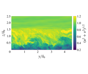
Speed cross-plane snapshot for (a) west to east and (b) east to west geostrophic velocity. The vertical domain extends to approximately  $3.5\unicode[STIX]{x1D6FF}_{0}$ and is truncated for visualization.

2.4 Conventionally neutral ABL with drag disk results
A cross-plane snapshot of the speed for the two simulations is shown in figure 3. Qualitatively, the boundary layer is significantly higher in the east to west geostrophic wind case. This is also shown in figure 4(a) where the peak of the sub-geostrophic jet is approximately  $16\,\%$ higher for the east to west geostrophic wind case. Further, as shown in figure 4(b), the peaks of $\overline{u^{\prime }w^{\prime }}$ are $17\,\%$ different. The veer profile is significantly different between the two geostrophic wind direction cases as shown in figure 4(c). Finally, the wind farm ABL logarithmic profile has changed as shown in figure 4(d). The friction velocities are $0.208\pm 0.0024$ and $0.218\pm 0.0031~\text{m}~\text{s}^{-1}$ in the west to east and east to west geostrophic direction cases respectively, representing a $5\,\%$ difference. The difference between $u^{\ast }$ in these two simulations is statistically significant ( $p<0.05$) according to a two-sample Kolmogorov–Smirnov statistical test. The influence of the geostrophic velocity direction has increased with the incorporation of inhomogeneous roughness elements in the form of drag disks.
The aforementioned influence of  $\unicode[STIX]{x1D6FA}_{y}$ on the boundary layer structure will change the interaction of the wind farm with the ABL. In particular, since the Reynolds stresses, mean velocities and boundary layer height are all affected, the mean transport of kinetic energy is influenced by the change in the direction of the geostrophic wind. These changes have resulted in differences in the magnitude of the wind turbine wakes, and therefore, the mean velocity at the hub heights of the drag disk wind turbine models. In the west to east geostrophic wind case, $(\overline{u}^{2}+\overline{v}^{2})^{1/2}/G=0.63$ while in the east to west geostrophic case $(\overline{u}^{2}+\overline{v}^{2})^{1/2}/G=0.66$. This represents a $4\,\%$ change in the mean speed at the wind turbine hub height as a result of the change in the direction of the geostrophic wind. However, the power in the wind is a cubic function of the wind speed $(P\sim u^{3})$. This is equivalent to a $12.5\,\%$ change in the power available at the drag disk model wind turbine hub height of 100 m. It is worth noting that this observation of the influence of $\unicode[STIX]{x1D6FA}_{y}$ on the power available at hub height is a coarse estimate of the true wind farm ABL due to the simplifications of the infinite wind farm, drag disk model wind turbines, and the conventionally neutral ABL.
The 36 drag disk model infinite wind farm simulation time and horizontally averaged (a) velocity, (b) Reynolds stresses, (c) wind direction and (d) wind speed. (a–c) Solid lines indicate west to east geostrophic wind and dashed lines indicate east to west geostrophic wind; (d) (blue ●) west to east geostrophic wind and (blue ▴) east to west geostrophic wind. The turbine locations are shown with dotted lines.

To study the effect of the geostrophic wind direction on vertical entrainment of kinetic energy, we first examine the evolution equation for the mean kinetic energy,
 $$\begin{eqnarray}\displaystyle \displaystyle \frac{\unicode[STIX]{x2202}}{\unicode[STIX]{x2202}t}\frac{1}{2}\overline{u}_{m}\overline{u}_{m} & = & \displaystyle -\frac{\unicode[STIX]{x2202}}{\unicode[STIX]{x2202}z}[(\overline{u}~\overline{u^{\prime }w^{\prime }}+\overline{v}~\overline{v^{\prime }w^{\prime }})+\left(\overline{u}~\overline{\unicode[STIX]{x1D70F}}_{13}+\overline{v}~\overline{\unicode[STIX]{x1D70F}}_{23}\right)]\nonumber\\ \displaystyle & & \displaystyle +\left[\overline{u^{\prime }w^{\prime }}{\displaystyle \frac{\unicode[STIX]{x2202}\overline{u}}{\unicode[STIX]{x2202}z}}+\overline{v^{\prime }w^{\prime }}{\displaystyle \frac{\unicode[STIX]{x2202}\overline{v}}{\unicode[STIX]{x2202}z}}\right]+\left[\overline{\unicode[STIX]{x1D70F}}_{13}{\displaystyle \frac{\unicode[STIX]{x2202}\overline{u}}{\unicode[STIX]{x2202}z}}+\overline{\unicode[STIX]{x1D70F}}_{23}{\displaystyle \frac{\unicode[STIX]{x2202}\overline{v}}{\unicode[STIX]{x2202}z}}\right]+\overline{u}\overline{f}+{\displaystyle \frac{2\unicode[STIX]{x1D6FA}_{z}}{Ro}}(\overline{v}G_{1}-\overline{u}G_{2}).\nonumber\\ \displaystyle & & \displaystyle\end{eqnarray}$$
 The time and horizontally averaged vertical velocity  $\overline{w}=0$ for all $z$. The horizontal component, $\unicode[STIX]{x1D6FA}_{y}$, does not explicitly appear in this balance. As such, differences between the two geostrophic wind direction cases will only manifest indirectly through other terms. As shown in figure 5(a), the convective transport has been significantly altered between the two cases. The convective transport is a function of the mean velocity profiles and the Reynolds stresses. The profiles for the mean velocities and Reynolds stresses are shown in figure 4. The terms in the TKE budget are shown in figure 5(b). In order to assess the role of the horizontal component more directly, we will calculate the Reynolds stress budgets. The $\overline{u^{\prime }w^{\prime }}$ momentum flux budget is given by
 $$\begin{eqnarray}\displaystyle \displaystyle \frac{\unicode[STIX]{x2202}\overline{u^{\prime }w^{\prime }}}{\unicode[STIX]{x2202}t} & = & \displaystyle -\frac{\unicode[STIX]{x2202}}{\unicode[STIX]{x2202}z}\left[\overline{u^{\prime }w^{\prime }w^{\prime }}+\overline{p^{\ast \prime }u^{\prime }}+\left(\overline{u^{\prime }\unicode[STIX]{x1D70F}_{33}}+\overline{w^{\prime }\unicode[STIX]{x1D70F}_{13}}\right)\right]+\overline{p^{\ast \prime }\left(\frac{\unicode[STIX]{x2202}w^{\prime }}{\unicode[STIX]{x2202}x}+\frac{\unicode[STIX]{x2202}u^{\prime }}{\unicode[STIX]{x2202}z}\right)}-\overline{w^{\prime }w^{\prime }}\frac{\unicode[STIX]{x2202}\overline{u}}{\unicode[STIX]{x2202}z}\nonumber\\ \displaystyle & & \displaystyle +\,\displaystyle \frac{1}{Fr^{2}}\overline{\unicode[STIX]{x1D703}^{\prime }u^{\prime }}+\left[\overline{\unicode[STIX]{x1D70F}_{3m}\frac{\unicode[STIX]{x2202}u^{\prime }}{\unicode[STIX]{x2202}x_{m}}}+\overline{\unicode[STIX]{x1D70F}_{1m}\frac{\unicode[STIX]{x2202}w^{\prime }}{\unicode[STIX]{x2202}x_{m}}}\right]\nonumber\\ \displaystyle & & \displaystyle +\,\overline{u^{\prime }f^{\prime }}-\frac{2}{Ro}(\unicode[STIX]{x1D6FA}_{y}\overline{w^{\prime }w^{\prime }}+\unicode[STIX]{x1D6FA}_{x}\overline{u^{\prime }v^{\prime }}-\unicode[STIX]{x1D6FA}_{z}\overline{v^{\prime }w^{\prime }}-\unicode[STIX]{x1D6FA}_{y}\overline{u^{\prime }u^{\prime }}).\end{eqnarray}$$
 The various terms that contribute to the budget equation are shown in figure 6(a). The dominating term in the Coriolis contribution is  $\unicode[STIX]{x1D6FA}_{y}\overline{u^{\prime }u^{\prime }}$, which is four times larger than any of the other terms in magnitude. The streamwise Reynolds stress $\overline{u^{\prime }u^{\prime }}$ is strictly positive in the domain and $\unicode[STIX]{x1D6FA}_{y}$ changes sign while keeping the same magnitude between the two simulations. As a result, the dominant term in the Coriolis source will change sign between the two simulations. Therefore, the $\overline{u^{\prime }w^{\prime }}$ Reynolds stress is a function of the direction of geostrophic wind provided that $\unicode[STIX]{x1D6FA}_{y}\overline{u^{\prime }u^{\prime }}$ is of similar magnitude to the other terms in the momentum flux budget.
The 36 drag disk model infinite wind farm simulation (a) mean kinetic energy and (b) turbulent kinetic energy budgets. Solid lines indicate west to east geostrophic wind and dashed lines indicate east to west geostrophic wind.

The momentum flux budget for  $\overline{v^{\prime }w^{\prime }}$ is shown in appendix A and similar observations can be made. The dominant term in the $\overline{v^{\prime }w^{\prime }}$ budget is less clear since $\overline{v^{\prime }v^{\prime }}$ is multiplied by $\unicode[STIX]{x1D6FA}_{x}$ which is less than $\unicode[STIX]{x1D6FA}_{y}$ in the present simulations. However, for northward geostrophic velocity, this term dominates the Coriolis source term in the momentum flux budget.
A more clear impact of the horizontal component ( $\unicode[STIX]{x1D6FA}_{y}$) is evident in the evolution equation for $\overline{w^{\prime }w^{\prime }}$ due to the absence of any direct shear production and actuator disk forcing
 $$\begin{eqnarray}\displaystyle \displaystyle \frac{\unicode[STIX]{x2202}\overline{w^{\prime }w^{\prime }}}{\unicode[STIX]{x2202}t} & = & \displaystyle -\frac{\unicode[STIX]{x2202}}{\unicode[STIX]{x2202}z}\left[\overline{w^{\prime }w^{\prime }w^{\prime }}+2\overline{p^{\ast \prime }w^{\prime }}+2\overline{w^{\prime }\unicode[STIX]{x1D70F}_{33}}\right]+\frac{2}{Fr^{2}}\overline{\unicode[STIX]{x1D703}^{\prime }w^{\prime }}\nonumber\\ \displaystyle & & \displaystyle +\,\displaystyle 2\overline{p^{\ast \prime }\frac{\unicode[STIX]{x2202}w^{\prime }}{\unicode[STIX]{x2202}z}}+2\overline{\unicode[STIX]{x1D70F}_{3m}\frac{\unicode[STIX]{x2202}w^{\prime }}{\unicode[STIX]{x2202}x_{m}}}-\frac{4}{Ro}(\unicode[STIX]{x1D6FA}_{x}\overline{v^{\prime }w^{\prime }}-\unicode[STIX]{x1D6FA}_{y}\overline{u^{\prime }w^{\prime }}).\end{eqnarray}$$
 The dominating term in the Coriolis contribution,  $\unicode[STIX]{x1D6FA}_{y}\overline{u^{\prime }w^{\prime }}$, changes sign while maintaining a similar magnitude in the two simulations. The various terms that contribute to the $\overline{w^{\prime }w^{\prime }}$ budget equation are shown in figure 6(b). Overall, $\unicode[STIX]{x1D6FA}_{y}>0$ of any magnitude will result in diminished turbulence energy levels while $\unicode[STIX]{x1D6FA}_{y}<0$ will only enhance turbulence energy up to a finite range which is likely a function of the local spanwise vorticity (Coleman et al. Reference Coleman, Ferziger and Spalart1990). Through this analysis, it is clear that the main direct effect of changing the direction of the geostrophic wind is to alter the Reynolds stress distribution in the ABL flow. With the Reynolds stresses, and particularly $\overline{u^{\prime }w^{\prime }}$, altered the mean statistics of the ABL will also have functional dependency on the direction of the geostrophic wind.
The 36 drag disk model infinite wind farm simulation (a)  $\overline{u^{\prime }w^{\prime }}$ and (b) $\overline{w^{\prime }w^{\prime }}$ budgets. Solid lines indicate west to east geostrophic wind and dashed lines indicate east to west geostrophic wind. The transport term is the summation of the turbulent, pressure and subfilter transports for the $\overline{u^{\prime }w^{\prime }}$ budget.

As noted by Zikanov et al. (Reference Zikanov, Slinn and Dhanak2003), the main influence of the geostrophic wind direction is in redistributing the individual components of turbulence kinetic energy through the Coriolis terms. Figure 7(a) shows the probability density functions of turbulent fluctuations for the two different geostrophic wind directions. The magnitude of turbulence fluctuations are larger in the east to west geostrophic velocity case. The  $u$-velocity two-point correlation at $0.6\unicode[STIX]{x1D6FF}_{0}$ is shown in figure 7(b). Further, the integral length scale of the $u$ velocity is larger in the east to west geostrophic case ( $0.69\unicode[STIX]{x1D6FF}_{0}$) than the west to east geostrophic case ( $0.31\unicode[STIX]{x1D6FF}_{0}$) as shown in the two-point correlations at $z=0.35\unicode[STIX]{x1D6FF}_{0}$ in figure 8(a). This location is approximately 150 m above the wind turbine hub height. The vertical location of interest is within the drag disk model shear layer above the disks. The correlation coefficients become zero valued well within the computational domain. The correlation coefficients are non-monotonic due to the three-dimensional wake and three-dimensional boundary layer structures.
(a) The turbine hub height joint probability density function  $P(u^{\prime },w^{\prime })$ and (b) the $u$ velocity two-point correlation at a height of $z=0.6\unicode[STIX]{x1D6FF}_{0}$. The black lines correspond to the west to east geostrophic wind and the red lines correspond to the east to west geostrophic wind. The red and black lines are at the same contour levels.

The 36 drag disk model periodic wind farm simulation has an aspect ratio of  $\text{L}_{x}\,:\,\text{L}_{y}$ of $2\,:\,1$ which is similar to previous conventionally neutral ABL simulations (see e.g. Allaerts & Meyers (Reference Allaerts and Meyers2015)). The streamwise and spanwise correlation coefficients for the west to east and east to west simulations at $z=0.35\unicode[STIX]{x1D6FF}_{0}$ are shown in figure 8(a,b).
The 36 drag disk model infinite wind farm simulation time and horizontally averaged (a) streamwise and (b) spanwise two-point correlation coefficient at a height of  $z=0.35\unicode[STIX]{x1D6FF}_{0}$. Solid lines indicate west to east geostrophic wind and dashed lines indicate east to west geostrophic wind.

A grid convergence study was performed to check that the observed dependency of the conventionally neutral ABL structure and statistics is not a function of the numerical resolution. The 36 drag disk model conventionally neutral ABL simulation was run with the same domain size but twice as coarse in all directions (256, 128 and 192 grid points in the  $x$,
$x$,  $y$ and $z$ directions, respectively). The high and low resolution simulations are compared in the mean velocity and Reynolds stress profiles in figure 9. The observed changes in the mean profiles as a function of grid refinement are less than the boundary layer structure and statistics changes as a function of the direction of the geostrophic wind. The influence of the grid resolution on the peak value of $\overline{u^{\prime }w^{\prime }}$ is $3\,\%$ while the influence of the direction of the geostrophic wind is $17\,\%$.
Grid convergence comparison for 36 drag disk model infinite wind farm simulation time and horizontally averaged (a) velocity and (b) Reynolds stresses. Both profiles are west to east geostrophic wind. Solid lines have two times as many grid points in each direction than the dotted lines.

2.5 Stable ABL
While the conventionally neutral ABL is a useful canonical flow due to its relative simplicity and comparability to the canonical engineering boundary layer (Allaerts & Meyers Reference Allaerts and Meyers2017), it is fundamentally an idealized flow which does not often occur in nature (Hess Reference Hess2004). Further, as also noted by Allaerts & Meyers (Reference Allaerts and Meyers2015), the quasi-stationary state discussed here takes an unrealistic amount of physical simulation time to reach from initialization. As such, we endeavour to evaluate the present results in the context of the more naturally occurring statically stable atmospheric boundary layer. To examine this state, we use the quasi-stationary conventionally neutral ABL simulations with drag disks as the initial conditions for a stable nocturnal boundary layer. A temporally varying surface heat flux of  $-0.003~\text{K}~\text{m}~\text{s}^{-1}$ per hour is imposed based on the diurnal cycle simulations of Kumar et al. (Reference Kumar, Kleissl, Meneveau and Parlange2006). The surface cooling heat flux is prescribed based on the HATS field experiment (Horst et al. Reference Horst, Kleissl, Lenschow, Meneveau, Moeng, Parlange, Sullivan and Weil2004; Kleissl, Parlange & Meneveau Reference Kleissl, Parlange and Meneveau2004). This flow is no longer statistically quasi-stationary in time. The friction velocities for the two stable ABL simulations are shown in figure 10.
Horizontally averaged friction velocity as a function of non-dimensional time ( $t^{\ast }=tG/\unicode[STIX]{x1D6FF}_{0}$) in the stable ABL with 36 drag disks.

The horizontally averaged velocity profiles two hours of physical time after the surface heat flux is imposed are shown in figure 11(a). The boundary layer height for the east to west geostrophic velocity case has remained significantly larger than the west to east case. Further, the structure of the turbulent fluctuations has remained different between the two cases as highlighted by the comparison of the fluctuation probability density functions at hub height shown in figure 11(b). The vertical fluctuations are less varied between the cases than in the conventionally neutral cases but there are significant differences between the horizontal fluctuations shown in figure 11(b) as a result of the geostrophic wind direction. This is likely due to the static stability’s effect of reducing the vertical velocity fluctuations and therefore  $\overline{w^{\prime }w^{\prime }}$. In the momentum flux budget for $\overline{w^{\prime }w^{\prime }}$, the buoyancy sink term begins to dominate the Coriolis source discrepancy for stable boundary layers. Figure 11(c,d) shows the horizontally averaged velocity profiles and the fluctuation probability density functions at hub height approximately four hours of physical time after the surface heat flux is imposed and similar conclusions can be made.
Previous simulations of the strongly statically stable case performed by Howland et al. (Reference Howland, Ghate and Lele2018) showed weak sensitivity to the geostrophic velocity direction. The strongly statically stable case was similar to the GEWEX Atmospheric Boundary Layer Study (GABLS) but at  $\unicode[STIX]{x1D719}=45^{\circ }$ while the standard GABLS case is at $\unicode[STIX]{x1D719}=73^{\circ }$ (Kosović & Curry Reference Kosović and Curry2000). However, in the present study, significant deviations between the two cases remain when initialized from the conventionally neutral ABL state. The sensitivity to the geostrophic wind direction is likely stronger in the present case than the GABLS case as a result of the lower Rossby number and weaker stable potential temperature lapse rate.
Wind farm dynamics is a function of the various stability regimes which occur in the ABL during a typical diurnal cycle (Hansen et al. Reference Hansen, Barthelmie, Jensen and Sommer2012; Fitch, Lundquist & Olson Reference Fitch, Lundquist and Olson2013). A number of recent studies have investigated wind turbine wakes (see e.g. Abkar, Sharifi & Porté-Agel (Reference Abkar, Sharifi and Porté-Agel2016) and Englberger & Dörnbrack (Reference Englberger and Dörnbrack2018)) during the diurnal cycle variations without considering the horizontal component of Earth’s rotation. Diurnal cycle simulations are typically initialized from a convective boundary layer base state (see e.g. Kumar et al. (Reference Kumar, Kleissl, Meneveau and Parlange2006)). The present results suggest that boundary layers transitioning between stability states may be a function of the static stability state of the initialization. While it has not been tested in the present study, sensitivity to the direction of the geostrophic velocity is expected in unstable boundary layers due to importance of  $\overline{w^{\prime }w^{\prime }}$.
(a) Horizontal velocities two hours after the negative surface heat flux is activated for west to east (solid) and east to west (dashed) geostrophic velocity. The turbine locations are shown with dotted lines. (b) The turbine hub height joint probability density function  $P(u^{\prime },w^{\prime })$. The black lines correspond to the west to east geostrophic wind and the red lines correspond to the east to west geostrophic wind. The red and black lines are at the same contour levels. (c,d) Same as (a,b) but four hours after the negative heat flux is activated.

3 Influence of drag disk spacing
In this section, we develop a simplified, quantitative model which approximates the influence of the horizontal component of Earth’s rotation on ABL flows with or without actuator disk models. The vertical transport of mean kinetic energy dictates the power production of large wind farms (Calaf et al. Reference Calaf, Meneveau and Meyers2010). The vertical transport of MKE is dictated by the shear Reynolds stresses  $\overline{u^{\prime }w^{\prime }}$ and $\overline{v^{\prime }w^{\prime }}$:
 $$\begin{eqnarray}-\frac{\unicode[STIX]{x2202}}{\unicode[STIX]{x2202}z}[(\overline{u}\overline{u^{\prime }w^{\prime }}+\overline{v}~\overline{v^{\prime }w^{\prime }})].\end{eqnarray}$$
 In the present simulations,  $\overline{u^{\prime }w^{\prime }}$ is significantly larger than $\overline{v^{\prime }w^{\prime }}$. As discussed in § 2, the horizontal component of Earth’s rotation $\unicode[STIX]{x1D6FA}_{y}$ primarily manifests as a source/sink term in the turbulent velocity covariance budgets. In particular, $\unicode[STIX]{x1D6FA}_{y}$ will directly influence the $\overline{u^{\prime }w^{\prime }}$ Reynolds stress through the Coriolis source/sink terms given in (2.8):
 $$\begin{eqnarray}-\frac{2}{Ro}(\unicode[STIX]{x1D6FA}_{y}\overline{w^{\prime }w^{\prime }}+\unicode[STIX]{x1D6FA}_{x}\overline{u^{\prime }v^{\prime }}-\unicode[STIX]{x1D6FA}_{z}\overline{v^{\prime }w^{\prime }}-\unicode[STIX]{x1D6FA}_{y}\overline{u^{\prime }u^{\prime }}).\end{eqnarray}$$
 The Coriolis terms in the respective velocity covariance budgets are also a function of the Reynolds stresses. When drag elements, or wind turbines, are placed in the ABL, the shear and normal stresses are significantly enhanced (see e.g. Calaf et al. (Reference Calaf, Meneveau and Meyers2010)). Additionally, drag elements and wind turbines generate wakes with enhanced turbulence which persist for  $10$ to $15D$ in ABL flows (Chamorro & Porté-Agel Reference Chamorro and Porté-Agel2009). The impact of the drag elements upon the boundary layer momentum balance is a function of their streamwise spacing and layout (Meneveau Reference Meneveau2012). Therefore, the influence of $\unicode[STIX]{x1D6FA}_{y}$ will be a function of the drag disk spacing.
To evaluate the influence of  $\unicode[STIX]{x1D6FA}_{y}$ as a function of drag disk spacing, we will utilize conventionally neutral ABL flows. With the precursor conventionally neutral ABL simulation described in § 2, drag disk elements are included with streamwise spacing of $S_{x}=8.5D$ and $S_{x}=4.25D$ and the spanwise spacing is fixed at $S_{y}=4.25D$. The $S_{x}=4.25D$ simulations are run with a domain height of 3.2 km to ensure that the boundary layer growth does not interfere with the top of the domain. The simulations are run until statistical quasi-stationarity as measured by $u^{\ast }$ is achieved. The Reynolds stresses associated with the vertical transport of kinetic energy are shown in figure 12(a). For both finite values of $S_{x}$, $\overline{u^{\prime }w^{\prime }}$ is enhanced in the east to west geostrophic case compared to the west to east geostrophic case. The difference in $\overline{u^{\prime }w^{\prime }}$ between the two geostrophic direction cases, denoted $\unicode[STIX]{x0394}\overline{u^{\prime }w^{\prime }}$, is higher for $S_{x}=4.25D$ than $S_{x}=8.5D$. The enhancement is also larger for $\overline{w^{\prime }w^{\prime }}$ in the $S_{x}=4.25D$ case, shown in figure 12(b). The convective transport terms (3.1) in each case are shown in figure 13 and similar observations can be made.
(a) Reynolds stresses  $\overline{u^{\prime }w^{\prime }}$ and $\overline{v^{\prime }w^{\prime }}$ for the simulations with $S_{x}=8.5D$ and $S_{x}=4.25D$. (b) Reynolds stresses $\overline{w^{\prime }w^{\prime }}$ for the simulations with $S_{x}=8.5D$ and $S_{x}=4.25D$. Solid lines indicate west to east geostrophic wind and dashed lines indicate east to west geostrophic wind. The turbine locations are shown with dotted lines.

Convective transport of mean kinetic energy for the (a) no turbine, (b) 36 turbine ( $S_{x}=8.5D$) and (c) 72 turbine ( $S_{x}=4.25D$) simulations. Solid lines indicate west to east geostrophic wind and dashed lines indicate east to west geostrophic wind. The turbine locations are shown with dotted lines.

The dominant Coriolis source/sink term in the  $\overline{u^{\prime }w^{\prime }}$ Reynolds stress equation ((2.8) and (3.2)) is $2(\unicode[STIX]{x1D714}\unicode[STIX]{x1D70F}\unicode[STIX]{x1D6FA}_{y})\overline{u^{\prime }u^{\prime }}$ where $\unicode[STIX]{x1D714}$ is the rotation of the Earth in radians per unit time and $\unicode[STIX]{x1D70F}$ is a relevant overturning time scale. The rotation of the Earth is $\unicode[STIX]{x1D714}=7.29\times 10^{-5}~\text{rad}~\text{s}^{-1}$ radians per second. The time scale used here is $\unicode[STIX]{x1D6FF}/G$, where $\unicode[STIX]{x1D6FF}$ is the boundary layer height in the simulation estimated as the location at which the boundary layer speed returns to the geostrophic velocity magnitude. The term $(\unicode[STIX]{x1D714}\unicode[STIX]{x1D70F}\unicode[STIX]{x0394}\unicode[STIX]{x1D6FA}_{y})$ uses the boundary layer height $\unicode[STIX]{x1D6FF}$ as the characteristic scale in the Rossby number. In the present study, $\unicode[STIX]{x1D70F}\approx 140~\text{s}$. Therefore, the impact of the change in geostrophic velocity forcing direction from west to east to east to west will change $\overline{u^{\prime }w^{\prime }}$ following
 $$\begin{eqnarray}\unicode[STIX]{x0394}\overline{u^{\prime }w^{\prime }}\sim 2(\unicode[STIX]{x1D714}\unicode[STIX]{x1D70F}\unicode[STIX]{x0394}\unicode[STIX]{x1D6FA}_{y})\overline{u^{\prime }u^{\prime }},\end{eqnarray}$$
 where  $\unicode[STIX]{x0394}\unicode[STIX]{x1D6FA}_{y}$ is the change in $\unicode[STIX]{x1D6FA}_{y}$ as a result of the different geostrophic velocity direction. Figure 14 shows $\overline{u^{\prime }u^{\prime }}$ and $\overline{v^{\prime }v^{\prime }}$ for the two streamwise spacing cases. The normal stresses are larger with streamwise spacing of $S_{x}=4.25D$ than $S_{x}=8.5D$, explaining the larger difference in shear stress $\unicode[STIX]{x0394}\overline{u^{\prime }w^{\prime }}$ (noted in figure 13). Both cases of drag disk spacing have considerably higher normal stresses in the boundary layer compared to the conventionally neutral ABL without drag disks shown in figure 14(a).
Reynolds stresses  $\overline{u^{\prime }u^{\prime }}$ and $\overline{v^{\prime }v^{\prime }}$ for the (a) no turbine, (b) 36 turbine ( $S_{x}=8.5D$) and (c) 72 turbine ( $S_{x}=4.25D$) simulations. Solid lines indicate west to east geostrophic wind and dashed lines indicate east to west geostrophic wind. The turbine locations are shown with dotted lines.

In order to approximate the influence of  $\unicode[STIX]{x1D6FA}_{y}$ on the vertical transport in the ABL, we can propose a model for (3.3). In the high Reynolds number atmospheric boundary layer, $\overline{u^{\prime }u^{\prime }}$ is directly related to $u^{\ast }$, the friction velocity. Following Stull (Reference Stull2012), in a conventionally neutral boundary layer, $\overline{u^{\prime }u^{\prime }}=ku^{\ast 2}$ in the surface layer, where $k=O(1)$. In a wind turbine atmospheric boundary layer, there is an upper and lower friction velocity due to the addition of roughness in the wind farm canopy. The value of $\overline{u^{\prime }u^{\prime }}$ can be related to the upper friction velocity, $u_{hi}^{\ast }$. According to the top-down model (Meneveau Reference Meneveau2012),
 $$\begin{eqnarray}u_{hi}^{\ast 2}=u^{\ast 2}+C_{T}(\unicode[STIX]{x03C0}D^{2}/4)[\overline{u}(z_{h})]^{2}\frac{1}{2S_{x}S_{y}D^{2}},\end{eqnarray}$$
 where  $C_{T}$ is the drag disk coefficient of thrust and $\overline{u}(z_{h})$ is horizontally averaged velocity at the turbine hub height in the ABL without turbines. Allaerts & Meyers (Reference Allaerts and Meyers2015) noted that the Coriolis forces must also be incorporated in the stress balance. Therefore, the change in the $\overline{u^{\prime }w^{\prime }}$ Reynolds stress at the turbine shear layer can be modelled as
 $$\begin{eqnarray}\unicode[STIX]{x0394}\overline{u^{\prime }w^{\prime }}_{m}=2k(\unicode[STIX]{x1D714}\unicode[STIX]{x1D70F}\unicode[STIX]{x0394}\unicode[STIX]{x1D6FA}_{y})u_{hi}^{\ast 2}.\end{eqnarray}$$
 The comparison of  $\unicode[STIX]{x0394}\overline{u^{\prime }w^{\prime }}$ from the precursor ABL and two drag disk spacing simulations with the model given by (3.5) is shown in table 1 with $k=2.5$.
The presently developed model can be used to assess the influence of the horizontal component of Earth’s rotation on  $\overline{u^{\prime }w^{\prime }}$. This model can be used to develop a coarse estimation for the impact of the horizontal component on the vertical transport in the ABL and the associated error in a calculation which invokes this assumption.
Top-down based model for the influence of the horizontal component of Earth’s rotation in the conventionally neutral ABL simulations without drag disks and with drag disk spacing of  $S_{x}=4.25D$ and $S_{x}=8.5D$. The model is given by (3.5). The percentage difference as a function of the maximum value of $\overline{u^{\prime }w^{\prime }}$ in the west to east geostrophic velocity simulation is shown in parenthesis.

4 Conclusions
The structure and statistics of the ABL are a function of the direction of the geostrophic wind due to the influence of the horizontal component of Earth’s rotation. The horizontal component of Earth’s rotation influences the conventionally neutral ABL statistics profiles, boundary layer height and friction velocity. The horizontal component also changes the structure of turbulence. This influence is enhanced when inhomogeneous wind turbine model drag disk roughness elements are incorporated in the ABL as a result of the enhanced normal Reynolds stresses and enhanced entrainment via vertical transport of mean kinetic energy. While the horizontal component of Earth’s rotation does not appear directly in the balance of turbulence kinetic energy, its influence persists through the momentum flux balances of Reynolds stresses.
Fundamentally, the horizontal component of Earth’s rotation influences the vertical balance of momentum. Neglecting the horizontal component of Earth’s rotation in the vertical momentum balance is commonplace (see e.g. Stull (Reference Stull2012)), justified on the basis of scaling with Rossby number. However, the horizontal component results in structural changes in the presently studied ABL for both conventionally neutral and statically stable ABLs with a realistic Rossby number. While LES of the ABL (Beare et al. Reference Beare, Macvean, Holtslag, Cuxart, Esau, Golaz, Jimenez, Khairoutdinov, Kosovic and Lewellen2006) and wind turbine models (Martinez-Tossas et al. Reference Martinez-Tossas, Churchfield, Yilmaz, Sarlak, Johnson, Sørensen, Meyers and Meneveau2018) are sensitive to modelling choices, the observed sensitivity of  $\overline{u^{\prime }w^{\prime }}$ to the direction of geostrophic wind is more significant than the observed sensitivity to the grid resolution, flow initialization, averaging window length and domain height. In particular, the sensitivity of the peak value of $\overline{u^{\prime }w^{\prime }}$ to the direction of the geostrophic wind in the conventionally neutral ABL is 10 %–16 % (see table 1), while the sensitivities to the domain height and the grid resolution are 0.05 % and 3 %, respectively. There are further modelling choices which have not been tested in the present study including subfilter scale and wall modelling, numerical scheme and others.
While neglecting the horizontal component may be justified in some geophysical flows, as Howland et al. (Reference Howland, Ghate and Lele2018) showed a weak sensitivity to the geostrophic wind direction in the GABLS case, it requires quantitative justification to do so. The influence of the horizontal component will at least be a function of the density stratification, Rossby number and boundary layer roughness. As such, quantitative arguments based on these flow quantities are required to rigorously justify neglecting this term.
The sensitivity to the direction of the geostrophic wind has been observed for simplified conventionally neutral and stable ABL cases with a periodic wind farm. Future work is required to evaluate this potential sensitivity in finite wind farm simulations as well as LES of the full diurnal cycle. Finally, field experiments should be conducted or the data should be reanalysed to evaluate whether such sensitivity can be observed in the boundary layer quantities of interest.
Acknowledgements
M.F.H. is funded through a National Science Foundation Graduate Research Fellowship under grant no. DGE-1656518 and a Stanford Graduate Fellowship. A.S.G. was funded by Tomkat Center for Sustainable Energy at Stanford University. All simulations were performed on Stampede2 supercomputer under the XSEDE project ATM170028. The authors would also like to thank the anonymous referees for their thoughtful comments and contribution to this work.
Declaration of interests
The authors report no conflict of interest.
Appendix A
A.1 Quasi-steadiness of the conventionally neutral ABL simulations
Due to the computational complexity of LES of finite sized model wind farms, precursor simulations are commonly used (Churchfield et al. Reference Churchfield, Lee, Michalakes and Moriarty2012; Stevens, Graham & Meneveau Reference Stevens, Graham and Meneveau2014). In the complex interaction between a wind farm and the ABL, it typically takes several flow through times to achieve statistical stationarity, even in the simplified periodic half-channel simulation environment (Calaf et al. Reference Calaf, Meneveau and Meyers2010). As such, in the present study, due to the large number of computationally expensive simulations required, a precursor simulation is used to initialize the conventionally neutral ABL state. LES of a conventionally neutral ABL without drag disk models is run until quasi-steady flow behaviour is achieved. This initialization reduces the number of flow through times required to reach quasi-steadiness for the various drag disk simulations that are performed in the present study. The precursor without drag disk models can also be analysed as a baseline comparison on the sensitivity of the conventionally neutral ABL case to the direction of the geostrophic wind.
The numerical set-up of the precursor simulation is given in § 2. The precursor simulation is initialized with uniform velocity with random noise added to the potential temperature profile. The simulation is run until quasi-steadiness is reached as measured by the friction velocity. The simulation is not statistically stationary due to inertial oscillations about the quasi-steady state. The friction velocity as a function of the non-dimensional time in the simulation is shown in figure 15.
(a) Friction velocity as a function of non-dimensional time in the conventionally neutral ABL without drag disks for west to east geostrophic wind with  $\unicode[STIX]{x1D6FA}_{y}\neq 0$ and $\unicode[STIX]{x1D6FA}_{y}=0$. The time $t^{\ast }=tG/\unicode[STIX]{x1D6FF}_{0}$ is non-dimensionalized by the geostrophic wind speed and the initial boundary layer height. (b) Same as (a) zoomed in for late simulation time.

The quasi-steadiness of all simulations are determined through the convergence of the mean of  $u^{\ast }$. As a result of inertial oscillations, the simulation is not strictly statistically stationary. The horizontally averaged velocity at 11 times during the time averaging window in the 36 wind turbine drag disk conventionally neutral ABL simulation discussed in § 2 is shown in figure 16. While there are inertial oscillations about the quasi-stationary state, the west to east and east to west geostrophic wind direction simulations remain dissimilar for all time steps.
Horizontally averaged velocity as a function of the wall normal height in the 36 drag disk conventionally neutral ABL simulations for 11 domain snapshots during the time-averaging window.

The mean profiles for the conventionally neutral ABL simulations presented in this study are horizontally and time averaged once  $u^{\ast }$ has converged to a quasi-steady value. The profiles were not significantly sensitive to the quantity of unique snapshots used during the time-averaging window (standard error of the mean has converged). Figure 17(a) shows the mean velocities in the conventionally neutral ABL profile for the case without turbines and $\unicode[STIX]{x1D6FA}_{y}=0$. Velocity profiles for time averaging considering 3000 ( $t^{\ast }=tG/\unicode[STIX]{x1D6FF}_{0}=106$) and 7000 ( $t^{\ast }=248$) unique time steps are compared. Both cases have time-averaging windows which are two orders of magnitude larger than the relevant time scale of the problem. The two mean velocity profiles show significantly less sensitivity as a result of the change in time-averaging length than as a result of the inclusion of $\unicode[STIX]{x1D6FA}_{y}\neq 0$. Similar observations can be made for the Reynolds stress profiles in figure 17(b). Thus, we can conclude that the influence of $\unicode[STIX]{x1D6FA}_{y}$ and the direction of the geostrophic wind observed in the present study is not due to insufficient time averaging nor statistical error.
Time and horizontally averaged (a) velocity and (b) Reynolds stresses for the conventionally neutral ABL simulations without drag disks and  $\unicode[STIX]{x1D6FA}_{y}=0$. The solid line is time averaged with 3000 unique time steps and the dashed line is time averaged with 7000 unique time steps.

A.2 Influence of the vertical domain height on the conventionally neutral boundary layer
The influence of the vertical domain height on the presently observed dependence of the conventionally neutral ABL to the direction of the geostrophic wind is tested. The conventionally neutral ABL without wind turbines is used from § 2. The domain presented in § 2 used an initial boundary layer height of  $\unicode[STIX]{x1D6FF}_{0}=700$ m and a domain extent of $L_{z}=2.4~\text{km}$. Rayleigh damping was enforced within the top $25\,\%$ of the domain. The simulation had $256$, $128$ and $192$ grid points in the $x$,
$x$,  $y$ and $z$ directions respectively.
In this section, we increase the domain extent to  $L_{z}=4.8~\text{km}$ and increase the vertical grid point number to $N_{z}=384$ to maintain the same grid spacing in the vertical direction. Figure 18 shows the velocities and Reynolds stresses for two simulations: west to east geostrophic wind with $L_{z}=4.8~\text{km}$ and west to east geostrophic wind with $L_{z}=2.4~\text{km}$. The two west to east geostrophic wind cases with $L_{z}=2.4$ and $L_{z}=4.8$ have the same velocities and Reynolds stresses as a function of height within the boundary layer. Therefore, we can confirm the selection of the vertical domain extent and Rayleigh damping in § 2. Therefore, we can confirm that the influence of the direction of the geostrophic wind observed in the present study is not a function of the domain height nor the Rayleigh damping enforced.
Conventionally neutral ABL simulation time and horizontally averaged (a) velocity and (b) Reynolds stresses without drag disk model wind turbines. The solid lines have a vertical domain extent of  $L_{z}=4.8~\text{km}$. The dotted lines have a vertical domain extent of $L_{z}=2.4~\text{km}$. Both simulations are for west to east geostrophic wind. The solid lines showing the results for the west to east taller domain simulations are virtually indistinguishable from the west to east simulations with half the vertical domain height (dots).

A.3 Transport and budget for  $\overline{v^{\prime }w^{\prime }}$

The  $\overline{v^{\prime }w^{\prime }}$ momentum flux budget is given by
 $$\begin{eqnarray}\displaystyle \displaystyle \frac{\unicode[STIX]{x2202}\overline{v^{\prime }w^{\prime }}}{\unicode[STIX]{x2202}t} & = & \displaystyle -\frac{\unicode[STIX]{x2202}}{\unicode[STIX]{x2202}z}\left[\overline{v^{\prime }w^{\prime }w^{\prime }}+\overline{p^{\ast \prime }v^{\prime }}+\left(\overline{v^{\prime }\unicode[STIX]{x1D70F}_{33}}+\overline{w^{\prime }\unicode[STIX]{x1D70F}_{23}}\right)\right]+\overline{p^{\ast \prime }\left(\frac{\unicode[STIX]{x2202}w^{\prime }}{\unicode[STIX]{x2202}y}+\frac{\unicode[STIX]{x2202}v^{\prime }}{\unicode[STIX]{x2202}z}\right)}-\overline{w^{\prime }w^{\prime }}\frac{\unicode[STIX]{x2202}\overline{v}}{\unicode[STIX]{x2202}z}\nonumber\\ \displaystyle & & \displaystyle +\displaystyle \frac{1}{Fr^{2}}\overline{\unicode[STIX]{x1D703}^{\prime }v^{\prime }}+\left[\overline{\unicode[STIX]{x1D70F}_{3m}\frac{\unicode[STIX]{x2202}v^{\prime }}{\unicode[STIX]{x2202}x_{m}}}+\overline{\unicode[STIX]{x1D70F}_{2m}\frac{\unicode[STIX]{x2202}w^{\prime }}{\unicode[STIX]{x2202}x_{m}}}\right]-\frac{2}{Ro}\left(\unicode[STIX]{x1D6FA}_{z}\overline{u^{\prime }w^{\prime }}+\unicode[STIX]{x1D6FA}_{x}\overline{v^{\prime }v^{\prime }}-\unicode[STIX]{x1D6FA}_{y}\overline{u^{\prime }v^{\prime }}-\unicode[STIX]{x1D6FA}_{x}\overline{w^{\prime }w^{\prime }}\right).\nonumber\\ \displaystyle & & \displaystyle\end{eqnarray}$$
 The various terms in the  $\overline{v^{\prime }w^{\prime }}$ momentum flux budget are shown for the 36 drag disk model infinite wind farm conventionally neutral ABL simulation in figure 19. Similar observations can be made as in § 2.
The 36 drag disk model infinite wind farm simulation  $\overline{v^{\prime }w^{\prime }}$ budget. Solid lines indicate west to east geostrophic wind and dashed lines indicate east to west geostrophic wind. The transport term is the summation of the turbulent, pressure and subfilter transports.

A.4 Normalized conventionally neutral boundary layer profiles
Given the observation that the direction of the geostrophic wind impacts the conventionally neutral ABL friction velocity and boundary layer height (§ 2.4), we will compare normalized boundary layer quantities. Boundary layer quantities in § 2.4 are normalized by the geostrophic wind speed and the coordinates are normalized by the initial boundary layer height in the simulation. The other relevant characteristic velocity in the ABL is the friction velocity. Figure 20(a) shows the speed as a function of the boundary layer height for the two geostrophic wind direction cases normalized by the temporally and horizontally averaged friction velocity. The speed profiles collapse in the near wall region, as expected, but diverge higher in the boundary layer where the velocity scale of interest is the geostrophic wind direction and inner normalization is not warranted. Additionally, figure 20(b) shows the speed profiles normalized by the geostrophic wind speed with the wall-normal coordinate normalized by the boundary layer height. The two geostrophic wind direction cases collapse in the free atmosphere but do not collapse in the boundary layer. Therefore, the observed discrepancies as a function of the direction of the geostrophic wind cannot be explained through these simple scaling laws but other scaling laws constructed on the basis of the enhanced or suppressed vertical transport of MKE as a function of the wind direction may be derived.
Conventionally neutral ABL simulation time and horizontally averaged speed with 36 drag disk model wind turbines with (a) the speed normalized by the temporally and horizontally averaged friction velocity and (b) the wall-normal coordinates normalized by the boundary layer height.


