


1 Introduction
Orbital angular momentum (OAM) is a fundamental property of light. Typically, OAM-carrying light can be categorized into spatial optical vortex pulses and spatiotemporal optical vortex (STOV) pulses based on their OAM orientation characteristics. The spatial optical vortices[
Reference Allen, Beijersbergen, Spreeuw and Woerdman1
,
Reference Yao and Padgett2
] propagating along the $x$
-axis exhibit monochromaticity and carry spiral phase profiles with the form of exp(
$x$
-axis exhibit monochromaticity and carry spiral phase profiles with the form of exp( $il\phi$
) in the transverse spatial plane (i.e.,
$il\phi$
) in the transverse spatial plane (i.e., $y-z$
plane), where
$y-z$
plane), where $l$
represents the topological charge (TC) and
$l$
represents the topological charge (TC) and $\phi$
is the azimuthal angle. Such a pulse possesses time-independent phase singularity and null intensity at the center, carrying longitudinal OAM parallel to the propagation direction with an OAM value of
$\phi$
is the azimuthal angle. Such a pulse possesses time-independent phase singularity and null intensity at the center, carrying longitudinal OAM parallel to the propagation direction with an OAM value of $l\mathrm{\hslash}$
per photon (
$l\mathrm{\hslash}$
per photon ( $\mathrm{\hslash}$
is the reduced Planck’s constant). Over the past three decades, these conventional spatial vortices underlying the extreme nonlinear process of high harmonic generation (HHG) and light–matter interactions enable the upconversion from visible and near-infrared to extreme ultraviolet (EUV)[
Reference Zhang, Shen, Shi, Wang, Zhang, Wang, Xu, Yi and Xu3
,
Reference Paufler, Böning and Fritzsche4
], X-ray[
Reference Hemsing, Knyazik, Dunning, Xiang, Marinelli, Hast and Rosenzweig5
–
Reference Schaap, Smorenburg and Luiten8
] and further to
$\mathrm{\hslash}$
is the reduced Planck’s constant). Over the past three decades, these conventional spatial vortices underlying the extreme nonlinear process of high harmonic generation (HHG) and light–matter interactions enable the upconversion from visible and near-infrared to extreme ultraviolet (EUV)[
Reference Zhang, Shen, Shi, Wang, Zhang, Wang, Xu, Yi and Xu3
,
Reference Paufler, Böning and Fritzsche4
], X-ray[
Reference Hemsing, Knyazik, Dunning, Xiang, Marinelli, Hast and Rosenzweig5
–
Reference Schaap, Smorenburg and Luiten8
] and further to $\gamma$
-ray regimes[
Reference Taira, Hayakawa and Katoh9
–
Reference Jiang, Zhuang, Chen, Li and Chen12
], which have attracted significant interest for broad interdisciplinary applications[
Reference Shen, Wang, Xie, Min, Fu, Liu, Gong and Yuan13
,
Reference Padgett14
].
$\gamma$
-ray regimes[
Reference Taira, Hayakawa and Katoh9
–
Reference Jiang, Zhuang, Chen, Li and Chen12
], which have attracted significant interest for broad interdisciplinary applications[
Reference Shen, Wang, Xie, Min, Fu, Liu, Gong and Yuan13
,
Reference Padgett14
].
By contrast, STOV pulses carrying pure transverse orbital angular momentum (TOAM) orthogonal to the propagation direction (i.e., $x$
-axis) exhibit intrinsic polychromatic and time-dependent phase singularities. These pulses feature spatiotemporal (ST) spiral wavefronts that rotate along the propagation axis, resembling a spinning bicycle wheel moving through the ST plane (i.e.,
$x$
-axis) exhibit intrinsic polychromatic and time-dependent phase singularities. These pulses feature spatiotemporal (ST) spiral wavefronts that rotate along the propagation axis, resembling a spinning bicycle wheel moving through the ST plane (i.e., $y-t$
plane)[
Reference Zhan15
–
Reference Porras20
]. This topology enables capabilities beyond the spatial OAM of conventional spatial optical vortices, such as intrinsic frequency-TC (
$y-t$
plane)[
Reference Zhan15
–
Reference Porras20
]. This topology enables capabilities beyond the spatial OAM of conventional spatial optical vortices, such as intrinsic frequency-TC ( $\omega -l$
) locking and temporal-shear interferometry, which promote spectral extension to higher frequencies. During the last decade, multiple sophisticated optical wave packets with ST vortices have been studied in a variety of aspects, such as their generation[
Reference Gui, Brooks, Kapteyn, Murnane and Liao21
–
Reference Liu, Cao, Zhang, Chong, Cai and Zhan28
], characterization[
Reference Gui, Brooks, Wang, Kapteyn, Murnane and Liao29
], propagation dynamics[
Reference Huang, Wang, Shen and Liu24
,
Reference Hancock, Zahedpour, Goffin and Milchberg30
–
Reference Song, Liu, Sun, Tong, Zhang, Cao, Wang, Huang, Zhang and Lu33
], diffraction[
Reference Chen, Zhang, Liu, Meng, Dudley and Lu27
,
Reference Huang, Wang, Shen, Liu and Li34
], reflection/refraction phenomena[
Reference Mazanov, Sugic, Alonso, Nori and Bliokh35
] and spin–orbit/orbit–orbit coupling[
Reference Bliokh36
–
Reference Chen, Zhao, Shen, Mo, Qiu and Zhan38
]. Remarkably, the spectral extension of STOV pulses has been achieved from the visible and near-infrared regimes to extreme wavelengths via HHG and relativistic light–matter interactions, which directly imprint the field’s ST structure and/or TOAM characteristics onto high-energy radiation[
Reference Dong, Xu, Fang, Ni, He, Zhuang and Liu25
,
Reference Fang, Lu and Liu39
–
Reference Sun, Wang, Dong, He, Shi, Lv, Zhan, Leng, Zhuang and Li49
]. This high-energy STOV light is essential for practical applications, such as high-resolution nanoscale imaging in crystallography[
Reference Nishino, Takahashi, Imamoto, Ishikawa and Maeshima50
,
Reference Schroer, Boye, Feldkamp, Patommel, Schropp, Schwab, Stephan, Burghammer, Schöder and Riekel51
], precise ST manipulation in ultrafast biophotonics[
Reference Hashimoto52
] and angular-momentum-resolved light–matter interactions in strong-field and quantum electrodynamics (QED) regimes[
Reference Sun, Wang, Dong, He, Shi, Lv, Zhan, Leng, Zhuang and Li49
].
$\omega -l$
) locking and temporal-shear interferometry, which promote spectral extension to higher frequencies. During the last decade, multiple sophisticated optical wave packets with ST vortices have been studied in a variety of aspects, such as their generation[
Reference Gui, Brooks, Kapteyn, Murnane and Liao21
–
Reference Liu, Cao, Zhang, Chong, Cai and Zhan28
], characterization[
Reference Gui, Brooks, Wang, Kapteyn, Murnane and Liao29
], propagation dynamics[
Reference Huang, Wang, Shen and Liu24
,
Reference Hancock, Zahedpour, Goffin and Milchberg30
–
Reference Song, Liu, Sun, Tong, Zhang, Cao, Wang, Huang, Zhang and Lu33
], diffraction[
Reference Chen, Zhang, Liu, Meng, Dudley and Lu27
,
Reference Huang, Wang, Shen, Liu and Li34
], reflection/refraction phenomena[
Reference Mazanov, Sugic, Alonso, Nori and Bliokh35
] and spin–orbit/orbit–orbit coupling[
Reference Bliokh36
–
Reference Chen, Zhao, Shen, Mo, Qiu and Zhan38
]. Remarkably, the spectral extension of STOV pulses has been achieved from the visible and near-infrared regimes to extreme wavelengths via HHG and relativistic light–matter interactions, which directly imprint the field’s ST structure and/or TOAM characteristics onto high-energy radiation[
Reference Dong, Xu, Fang, Ni, He, Zhuang and Liu25
,
Reference Fang, Lu and Liu39
–
Reference Sun, Wang, Dong, He, Shi, Lv, Zhan, Leng, Zhuang and Li49
]. This high-energy STOV light is essential for practical applications, such as high-resolution nanoscale imaging in crystallography[
Reference Nishino, Takahashi, Imamoto, Ishikawa and Maeshima50
,
Reference Schroer, Boye, Feldkamp, Patommel, Schropp, Schwab, Stephan, Burghammer, Schöder and Riekel51
], precise ST manipulation in ultrafast biophotonics[
Reference Hashimoto52
] and angular-momentum-resolved light–matter interactions in strong-field and quantum electrodynamics (QED) regimes[
Reference Sun, Wang, Dong, He, Shi, Lv, Zhan, Leng, Zhuang and Li49
].
However, existing schemes for generating OAM-related high-energy radiation beyond the EUV region model the radiation photons as plane waves carrying collective OAM only in the statistical sense, typically yielding only incoherent emission[ Reference Jiang, Zhuang, Chen, Li and Chen12 , Reference Zhang, Zhang and Xie47 , Reference Sun, Wang, Dong, He, Shi, Lv, Zhan, Leng, Zhuang and Li49 , Reference Chen, Li, Hatsagortsyan and Keitel53 , Reference Zhu, Yu, Chen, Weng and Sheng54 ], thereby preventing the formation of structured fields (such as donut-shaped intensity distributions and spiral phase profiles). To date, no coherent mode-resolved STOV pulse with a well-defined ST field structure has been demonstrated beyond the EUV band. Very recently, STOV pulses were employed to produce isolate, ultrabright attosecond X-ray pulses from a thin foil[ Reference Ju, Wu, Yu, Huang, Zhang, Wu, Zhou and Ruan55 ]. However, conclusive evidence confirming the presence of TOAM in these X-ray pulses is still lacking. Therefore, the generation of mode-resolved STOV pulses in the X-ray range with well-defined ST field structures constitutes an open and largely unexplored challenge.
In this work, we demonstrate a viable route for generating coherent X-ray STOV harmonics through nonlinear Thomson scattering. This is achieved via a head-on collision between an intense STOV pulse and a nanometer-scale relativistic electron beam at the focal region; see Figure 1(a). The simulation results by the far-field time-domain radiation scheme (Figure 1(b)) reveal the emission of high-frequency radiation carrying well-defined STOV structures in the X-ray domain. The vortex charges of resulting harmonic emissions scale with the harmonic order, consistent with the TOAM conservation law. Crucially, the formation of such STOV-structured radiation relies on precise temporal synchronization, spatial confinement and ST phase matching among the emitting electrons. Without these, spectral broadening and angular dispersion disrupt the interference pattern, rendering the STOV field structures unobservable. The results open new possibilities for developing high brightness, angular-momentum mode-resolved X-ray and even $\gamma$
-ray sources with attosecond-scale temporal resolution.
$\gamma$
-ray sources with attosecond-scale temporal resolution.
Scheme for generating coherent, mode-resolved STOV harmonics in the X-ray regime via nonlinear Thomson scattering. (a) Schematic of the X-ray STOV generation process, where a near-infrared STOV pulse ( ${\lambda}_0=1\;\mu \mathrm{m},\tau =2{t}_{\mathrm{p}}$
) head-on collides with a relativistic electron beam (initial electron energy
${\lambda}_0=1\;\mu \mathrm{m},\tau =2{t}_{\mathrm{p}}$
) head-on collides with a relativistic electron beam (initial electron energy ${\varepsilon}_0=2.56$
MeV) with a longitudinal thickness of 1 nm. (b) Geometry of the far-field time-domain radiation calculation; see the main text for more details.
${\varepsilon}_0=2.56$
MeV) with a longitudinal thickness of 1 nm. (b) Geometry of the far-field time-domain radiation calculation; see the main text for more details.

2 Scheme and simulation method
We employ a linearly $y$
-polarized STOV beam with vortex charge
$y$
-polarized STOV beam with vortex charge $l=1$
and central wavelength
$l=1$
and central wavelength ${\lambda}_0=1\kern0.22em \mu \mathrm{m}$
. The normalized laser amplitude is set to be
${\lambda}_0=1\kern0.22em \mu \mathrm{m}$
. The normalized laser amplitude is set to be ${{a}_0={eE}_0/{m}_{\mathrm{e}}c{\omega}_0=1}$
, where
${{a}_0={eE}_0/{m}_{\mathrm{e}}c{\omega}_0=1}$
, where ${E}_0$
is the peak electric field,
${E}_0$
is the peak electric field, $e$
and
$e$
and ${m}_{\mathrm{e}}$
are the elementary charge and electron mass, respectively, and
${m}_{\mathrm{e}}$
are the elementary charge and electron mass, respectively, and ${\omega}_0$
is the central laser frequency. The intensity profile of an STOV pulse propagating along the
${\omega}_0$
is the central laser frequency. The intensity profile of an STOV pulse propagating along the $x$
-axis undergoes an evolution from a donut-shaped distribution into spatiotemporally offset lobes. Accordingly, the
$x$
-axis undergoes an evolution from a donut-shaped distribution into spatiotemporally offset lobes. Accordingly, the $y$
-component of the vector potential is derived as follows[
Reference Wang, Chen, Zhang and Shen40
,
Reference Hancock, Zahedpour and Milchberg56
]:
$y$
-component of the vector potential is derived as follows[
Reference Wang, Chen, Zhang and Shen40
,
Reference Hancock, Zahedpour and Milchberg56
]:
 $$\begin{align} &{u}_y^{l=1}\left(y,z,\xi \right)={A}_0\sqrt{\frac{w_{y0}{w}_{z0}}{w_y(x){w}_z(x)}}\left(\frac{iye^{-i{\psi}_y}}{w_y(x)}+\frac{\xi }{w_{\xi }}\right)\nonumber\\ &\quad{}\times \exp \left(-\frac{y^2}{w_y^2(x)}-\frac{z^2}{w_z^2(x)}-\frac{\xi^2}{w_{\xi}^2}\right)\exp \left(\frac{-i{\psi}_y-i{\psi}_z}{2}\right)\nonumber\\ &\quad{}\times \exp \left(-\frac{ik_0{z}^2}{R_z}-\frac{ik_0{y}^2}{R_y}\right)\exp \left({ik}_0\xi \right),\end{align}$$
where ${A}_0$
is the peak amplitude of the vector potential and i is the imaginary unit. The beam waists evolve with propagation as
${A}_0$
is the peak amplitude of the vector potential and i is the imaginary unit. The beam waists evolve with propagation as ${w}_y(x)={w}_{y0}\sqrt{1+{\left(x/{x}_{0y}\right)}^2}$
and
${w}_y(x)={w}_{y0}\sqrt{1+{\left(x/{x}_{0y}\right)}^2}$
and ${w}_z(x)={w}_{z0}\sqrt{1+{\left(x/{x}_{0z}\right)}^2}$
, where
${w}_z(x)={w}_{z0}\sqrt{1+{\left(x/{x}_{0z}\right)}^2}$
, where ${w}_{y0}={w}_{z0}=2\ \mu \mathrm{m}$
, and the corresponding Rayleigh ranges are
${w}_{y0}={w}_{z0}=2\ \mu \mathrm{m}$
, and the corresponding Rayleigh ranges are ${x}_{0y}={k}_0{w}_{y0}^2/2$
and
${x}_{0y}={k}_0{w}_{y0}^2/2$
and ${x}_{0z}={k}_0{w}_{z0}^2/2$
with
${x}_{0z}={k}_0{w}_{z0}^2/2$
with ${k}_0$
being the wave vector. Here,
${k}_0$
being the wave vector. Here, ${R}_y=x\left(1+{\left({x}_{0y}/x\right)}^2\right)$
and
${R}_y=x\left(1+{\left({x}_{0y}/x\right)}^2\right)$
and ${R}_z=x\left(1+{\left({x}_{0z}/x\right)}^2\right)$
denote the beam curvature radii along the
${R}_z=x\left(1+{\left({x}_{0z}/x\right)}^2\right)$
denote the beam curvature radii along the $y$
- and
$y$
- and $z$
-axes, respectively. The corresponding transverse Gouy phase shifts are defined as
$z$
-axes, respectively. The corresponding transverse Gouy phase shifts are defined as ${\psi}_y=\arctan \left(x/{x}_{0y}\right)$
and
${\psi}_y=\arctan \left(x/{x}_{0y}\right)$
and ${\psi}_z=\arctan \left(x/{x}_{0z}\right)$
, among which
${\psi}_z=\arctan \left(x/{x}_{0z}\right)$
, among which ${\psi}_y$
dominates the propagation-driven evolution of the STOV field’s intensity profile from a donut configuration to an elliptical STOV structure then to spatiotemporally offset lobes[
Reference Hancock, Zahedpour and Milchberg56
]. The ST coupling coordinate is defined as
${\psi}_y$
dominates the propagation-driven evolution of the STOV field’s intensity profile from a donut configuration to an elliptical STOV structure then to spatiotemporally offset lobes[
Reference Hancock, Zahedpour and Milchberg56
]. The ST coupling coordinate is defined as $\xi = ct-x$
, and the temporal envelope of the beam is characterized by a Gaussian profile with width
$\xi = ct-x$
, and the temporal envelope of the beam is characterized by a Gaussian profile with width ${w}_{\xi }$
, corresponding to a pulse duration of
${w}_{\xi }$
, corresponding to a pulse duration of ${w}_{\xi }/c=2{t}_{\mathrm{p}}$
, where
${w}_{\xi }/c=2{t}_{\mathrm{p}}$
, where ${t}_{\mathrm{p}}={\lambda}_0/c=3.3\ \mathrm{fs}$
is the laser period.
${t}_{\mathrm{p}}={\lambda}_0/c=3.3\ \mathrm{fs}$
is the laser period.
In our configuration, the STOV–electron collision is centered at the focus and the interaction region is much shorter than the Rayleigh length, so the electrons predominantly sample the near-focus part of the field, where the elliptical STOV structure is indeed realized. During this short interaction, the driving pulse does not have time to evolve into the far-field ST tilted-Hermite lobe (ST-THL) pattern. Nevertheless, the full $x$
-dependent STOV field is implemented in the code and used to compute both the electron trajectories and the corresponding Liénard–Wiechert radiation fields. The beam exhibits Laguerre-Gaussian (LG)-like profiles in the spatial and temporal plane (i.e.,
$x$
-dependent STOV field is implemented in the code and used to compute both the electron trajectories and the corresponding Liénard–Wiechert radiation fields. The beam exhibits Laguerre-Gaussian (LG)-like profiles in the spatial and temporal plane (i.e., $y-\xi$
plane). At the focal plane, transverse Gouy phase shifts are absent. Accordingly, the generalized radial coordinate and vortex phase of the STOV field are respectively defined as follows:
$y-\xi$
plane). At the focal plane, transverse Gouy phase shifts are absent. Accordingly, the generalized radial coordinate and vortex phase of the STOV field are respectively defined as follows:
 $$\begin{align}\tilde{r}=\sqrt{{\left(\frac{y}{w_y(x)}\right)}^2+{\left(\frac{\xi }{w_{\xi }}\right)}^2},\kern1em \tilde{\phi}=\arctan \left(\frac{yw_{\xi }}{\xi {w}_y(x)}\right).\end{align}$$
At the beam focus (i.e., $x=0$
), the intensity distribution becomes circularly symmetric in the
$x=0$
), the intensity distribution becomes circularly symmetric in the $y$
–
$y$
– $\xi$
plane provided
$\xi$
plane provided ${w}_{y0}={w}_{\xi }$
. In this case, the radial and azimuthal coordinates reduce to the following:
${w}_{y0}={w}_{\xi }$
. In this case, the radial and azimuthal coordinates reduce to the following:
 $$\begin{align}\tilde{r}\propto \sqrt{y^2+{\xi}^2},\kern1em \tilde{\phi}=\arctan \left(\frac{y}{\xi}\right),\end{align}$$
resulting in a donut-shaped intensity profile centered at the origin. When it is away from the focal plane, the isointensity contours become tilted due to diffraction and ST coupling[
Reference Hancock, Zahedpour and Milchberg56
], as illustrated in Figure 1(a). The field amplitude exhibits a downward fork-like pattern, governed by the sign of the carrier phase term in Equation (1). The associated electric and magnetic fields can be calculated from ${u}_y^{l=1}$
via the following[
Reference Arora and Lu57
]:
${u}_y^{l=1}$
via the following[
Reference Arora and Lu57
]:
 $$\begin{align}\vec{E}={ik}_0\vec{u}-\frac{i}{k_0}\nabla \left(\nabla \cdot \vec{u}\right),\end{align}$$
 $$\begin{align}\vec{B}=\nabla \times \vec{u}.\end{align}$$
The electron beam consists of $2\times {10}^4$
electrons initially confined within a cylindrical volume with a longitudinal thickness of 1 nm. The electrons follow a random spatial distribution with a transverse Gaussian profile described by the following:
$2\times {10}^4$
electrons initially confined within a cylindrical volume with a longitudinal thickness of 1 nm. The electrons follow a random spatial distribution with a transverse Gaussian profile described by the following:
 $$\begin{align}f\left(y,z\right)=\frac{1}{2{\pi \sigma}_y{\sigma}_z}\exp \left(-\frac{y^2}{2{\sigma}_y^2}-\frac{z^2}{2{\sigma}_z^2}\right).\end{align}$$
To ensure full collision between the STOV light and the electron beam, the electron beam is confined within a circular region of a radius $r=4{\lambda}_0$
, with corresponding root-mean-square (rms) widths of
$r=4{\lambda}_0$
, with corresponding root-mean-square (rms) widths of ${\sigma}_y={\sigma}_z=2.5{\lambda}_0$
. The initial electron energy is
${\sigma}_y={\sigma}_z=2.5{\lambda}_0$
. The initial electron energy is ${\varepsilon}_0=2.56$
MeV (corresponding to
${\varepsilon}_0=2.56$
MeV (corresponding to $\gamma =5$
). In our simulations here, we neglect the energy spread and divergence angle, that is,
$\gamma =5$
). In our simulations here, we neglect the energy spread and divergence angle, that is, $\Delta \gamma /\gamma =0,\ \Delta \beta =0$
[
Reference Lee, Kim and Kim58
,
Reference Pausch, Debus, Huebl, Schramm, Steiniger, Widera and Bussmann59
]. In addition, to quantitatively assess the impact of energy spread on the generated harmonic spectrum, we conducted dedicated follow-up simulations for electron beams with energy spreads of 0.1
$\Delta \gamma /\gamma =0,\ \Delta \beta =0$
[
Reference Lee, Kim and Kim58
,
Reference Pausch, Debus, Huebl, Schramm, Steiniger, Widera and Bussmann59
]. In addition, to quantitatively assess the impact of energy spread on the generated harmonic spectrum, we conducted dedicated follow-up simulations for electron beams with energy spreads of 0.1 $\%$
, 0.3
$\%$
, 0.3 $\%$
and 0.5
$\%$
and 0.5 $\%$
; see Appendix A for more details. Furthermore, in the traditional Thomson scattering mechanism, under conditions of low electron beam density (
$\%$
; see Appendix A for more details. Furthermore, in the traditional Thomson scattering mechanism, under conditions of low electron beam density ( $<{10}^{24}\ {\mathrm{m}}^{-3}$
), short interaction time or weak laser intensity, the inter-electron Coulomb fields are far weaker than the laser field, and their effects on electron dynamics and radiation are negligible[
Reference Jackson and Fox60
]. In our scheme, the electron beam density employed is of the order of
$<{10}^{24}\ {\mathrm{m}}^{-3}$
), short interaction time or weak laser intensity, the inter-electron Coulomb fields are far weaker than the laser field, and their effects on electron dynamics and radiation are negligible[
Reference Jackson and Fox60
]. In our scheme, the electron beam density employed is of the order of ${10}^{23}\ {\mathrm{m}}^{-3}$
, which is well below the critical density threshold for significant Coulomb effects, meaning the Coulomb interaction can be safely neglected. This approximation is widely adopted in the laser–electron interaction frameworks[
Reference Lee, Kim and Kim58
,
Reference Pausch, Debus, Huebl, Schramm, Steiniger, Widera and Bussmann59
,
Reference Li, Shaisultanov, Hatsagortsyan, Wan, Keitel and Li61
], further validating its rationality in our work. Nanometer-scale relativistic electron beams have been experimentally achieved via laser–foil interactions[
Reference Meyer-ter Vehn and Wu62
], and alternatively, attosecond electron sheets have been generated and phase-locked to relativistic energies[
Reference Sun, Wang, Dong, He, Shi, Lv, Zhan, Leng, Zhuang and Li49
,
Reference Hu, Yu, Cao, Chen, Zou, Yin, Sheng and Shao63
,
Reference Wu, Meyer-ter Vehn, Fernández and Hegelich64
].
${10}^{23}\ {\mathrm{m}}^{-3}$
, which is well below the critical density threshold for significant Coulomb effects, meaning the Coulomb interaction can be safely neglected. This approximation is widely adopted in the laser–electron interaction frameworks[
Reference Lee, Kim and Kim58
,
Reference Pausch, Debus, Huebl, Schramm, Steiniger, Widera and Bussmann59
,
Reference Li, Shaisultanov, Hatsagortsyan, Wan, Keitel and Li61
], further validating its rationality in our work. Nanometer-scale relativistic electron beams have been experimentally achieved via laser–foil interactions[
Reference Meyer-ter Vehn and Wu62
], and alternatively, attosecond electron sheets have been generated and phase-locked to relativistic energies[
Reference Sun, Wang, Dong, He, Shi, Lv, Zhan, Leng, Zhuang and Li49
,
Reference Hu, Yu, Cao, Chen, Zou, Yin, Sheng and Shao63
,
Reference Wu, Meyer-ter Vehn, Fernández and Hegelich64
].
In our simulation, electron trajectories are computed by numerically solving the relativistic equations of motion using a fourth-order Runge–Kutta method. At each time step, the positions, velocities and local field quantities of all electrons are recorded. These trajectories are subsequently passed to the far-field time-domain (FaTiDo) simulation code[
Reference Peng, Huang, Jiang, Li, Wu, Yu, Riconda, Weber, Zhou and Ruan65
], which computes three-dimensional far-field radiation based on the Liénard–Wiechert potentials[
Reference Jackson and Fox60
]. The FaTiDo implementation has been benchmarked against the Osiris radio module[
Reference Pardal, Sainte-Marie, Reboul-Salze, Fonseca and Vieira66
,
Reference Vieira, Pardal, Mendonça and Fonseca67
], as well as established models of terahertz emission from superluminal sources and nonlinear Thomson scattering[
Reference Taira, Hayakawa and Katoh9
,
Reference Pausch, Debus, Widera, Steiniger, Huebl, Burau, Bussmann and Schramm68
]. The radiation is projected onto a spherical detector surface located at $R=1\kern0.22em \mathrm{m}$
from the interaction center, as illustrated in Figure 1(b). The detector covers polar angles
$R=1\kern0.22em \mathrm{m}$
from the interaction center, as illustrated in Figure 1(b). The detector covers polar angles $\theta \in \left[-10,10\right]\;\mathrm{mrad}$
and azimuthal angles
$\theta \in \left[-10,10\right]\;\mathrm{mrad}$
and azimuthal angles $\varphi \in \left[0,2\pi \right]$
, discretized into
$\varphi \in \left[0,2\pi \right]$
, discretized into ${N}_{\theta}\times {N}_{\varphi }=64\times 128$
observation points. The temporal axis is sampled with a step size of
${N}_{\theta}\times {N}_{\varphi }=64\times 128$
observation points. The temporal axis is sampled with a step size of $\mathrm{d}t=0.5\;\mathrm{as}$
over
$\mathrm{d}t=0.5\;\mathrm{as}$
over ${N}_t=4000$
steps, enabling ultrashort and high-frequency resolution.
${N}_t=4000$
steps, enabling ultrashort and high-frequency resolution.
The radiation (far-field) expression from the $m$
th electron at an observation point
$m$
th electron at an observation point $\left(\theta, \varphi \right)$
and arrival time
$\left(\theta, \varphi \right)$
and arrival time ${t}_{\mathrm{det}}$
is given by the Liénard–Wiechert expression[
Reference Peng, Huang, Jiang, Li, Wu, Yu, Riconda, Weber, Zhou and Ruan65
]:
${t}_{\mathrm{det}}$
is given by the Liénard–Wiechert expression[
Reference Peng, Huang, Jiang, Li, Wu, Yu, Riconda, Weber, Zhou and Ruan65
]:
 $$\begin{align}{\vec{E}}_{m,\det}\left(\theta, \varphi, {t}_{\mathrm{det}}\right)=\frac{e}{4{\pi \varepsilon}_0{c}^2}\frac{\vec{n}\times \left(\left(\vec{n}-\vec{\beta}\right)\times \dot{\vec{\beta}}\right)}{{\left(1-\vec{n}\cdot \vec{\beta}\right)}^3R},\end{align}$$
 $$\begin{align}{\vec{B}}_{m,\det}\left(\theta, \varphi, {t}_{\mathrm{det}}\right)=\frac{\vec{n}}{c}\times {\vec{E}}_{m,\det}\left(\theta, \varphi, {t}_{\mathrm{det}}\right).\end{align}$$
This ignores the near-field component, which decreases inversely with the square of the distance ${R}^{-2}$
[
Reference Pausch69
]. The radiation component is adopted to calculate the observable emission and inherently incorporates the full propagation of the radiated wave from the moving charge to the detector. This propagation mechanism is fundamentally distinct from the free-space evolution of the driving STOV pulse. The STOV field affects the emission exclusively via the Lorentz force that shapes electron trajectories; once radiation is emitted, its angular and spectral structure is governed solely by Liénard–Wiechert dynamics, rather than the STOV’s intrinsic ST-THLs
${R}^{-2}$
[
Reference Pausch69
]. The radiation component is adopted to calculate the observable emission and inherently incorporates the full propagation of the radiated wave from the moving charge to the detector. This propagation mechanism is fundamentally distinct from the free-space evolution of the driving STOV pulse. The STOV field affects the emission exclusively via the Lorentz force that shapes electron trajectories; once radiation is emitted, its angular and spectral structure is governed solely by Liénard–Wiechert dynamics, rather than the STOV’s intrinsic ST-THLs $\to$
donut-STOVs
$\to$
donut-STOVs $\to$
ST-THLs propagation cycle[
Reference Hancock, Zahedpour and Milchberg56
]. This point is conceptually critical when making comparisons with the HHG scenario of Ref. [Reference Martín-Hernández, Gui, Plaja, Kapteyn, Murnane, Liao, Porras and Hernández-García45]. In HHG, the harmonics inherit the complete STOV phase at the generation point and then propagate as independent optical beams, which naturally evolve into ST-THL structures in the far-field. In contrast, in our relativistic scattering configuration, the vortex features of the high-frequency emission are encoded in the ensemble of electron trajectories and their Liénard–Wiechert radiation. In the parameter regime considered, this yields a quasi-elliptical angular distribution at high frequencies – fully consistent with the radiation mechanism of accelerated charges, and one that does not contradict the well-established propagation behavior of a freely propagating STOV beam. Here,
$\to$
ST-THLs propagation cycle[
Reference Hancock, Zahedpour and Milchberg56
]. This point is conceptually critical when making comparisons with the HHG scenario of Ref. [Reference Martín-Hernández, Gui, Plaja, Kapteyn, Murnane, Liao, Porras and Hernández-García45]. In HHG, the harmonics inherit the complete STOV phase at the generation point and then propagate as independent optical beams, which naturally evolve into ST-THL structures in the far-field. In contrast, in our relativistic scattering configuration, the vortex features of the high-frequency emission are encoded in the ensemble of electron trajectories and their Liénard–Wiechert radiation. In the parameter regime considered, this yields a quasi-elliptical angular distribution at high frequencies – fully consistent with the radiation mechanism of accelerated charges, and one that does not contradict the well-established propagation behavior of a freely propagating STOV beam. Here, $\vec{n}=\left({\vec{r}}_{\mathrm{det}}-{\vec{r}}_{\mathrm{e}}\right)/\mid\kern-1.2pt {\vec{r}}_{\mathrm{det}}-{\vec{r}}_{\mathrm{e}}\kern-1.7pt\mid$
is the unit vector from the electron to the detector point,
$\vec{n}=\left({\vec{r}}_{\mathrm{det}}-{\vec{r}}_{\mathrm{e}}\right)/\mid\kern-1.2pt {\vec{r}}_{\mathrm{det}}-{\vec{r}}_{\mathrm{e}}\kern-1.7pt\mid$
is the unit vector from the electron to the detector point, $\vec{\beta}=\vec{v}/c$
is the normalized velocity and
$\vec{\beta}=\vec{v}/c$
is the normalized velocity and $\dot{\vec{\beta}}=\mathrm{d}\vec{\beta }/\mathrm{d}t$
is the normalized acceleration. The detector arrival time is related to the retarded time by the following:
$\dot{\vec{\beta}}=\mathrm{d}\vec{\beta }/\mathrm{d}t$
is the normalized acceleration. The detector arrival time is related to the retarded time by the following:
 $$\begin{align}{t}_{\mathrm{det}}={t}_{\mathrm{ret}}+\frac{\mid {\vec{r}}_{\mathrm{det}}-{\vec{r}}_{\mathrm{e}}\left({t}_{\mathrm{ret}}\right)\mid }{c}.\end{align}$$
Because ${t}_{\mathrm{ret}}$
is nonuniformly sampled, the radiation fields are interpolated onto a uniform detector time grid following the algorithm in Ref. [Reference Pardal, Sainte-Marie, Reboul-Salze, Fonseca and Vieira66]. The total far-field radiation is then obtained by coherently summing contributions from all
${t}_{\mathrm{ret}}$
is nonuniformly sampled, the radiation fields are interpolated onto a uniform detector time grid following the algorithm in Ref. [Reference Pardal, Sainte-Marie, Reboul-Salze, Fonseca and Vieira66]. The total far-field radiation is then obtained by coherently summing contributions from all ${{N}_{\mathrm{e}}=2\times {10}^4}$
accelerated electrons, with each term carrying the complex phase
${{N}_{\mathrm{e}}=2\times {10}^4}$
accelerated electrons, with each term carrying the complex phase ${\chi}_m=\exp \left( i\omega \left(t-\vec{n}\cdot {\vec{r}}_{\mathrm{e}}\right)/c\right)$
[
Reference Pausch, Debus, Huebl, Schramm, Steiniger, Widera and Bussmann59
], that is
${\chi}_m=\exp \left( i\omega \left(t-\vec{n}\cdot {\vec{r}}_{\mathrm{e}}\right)/c\right)$
[
Reference Pausch, Debus, Huebl, Schramm, Steiniger, Widera and Bussmann59
], that is
 $$\begin{align}{\vec{E}}_{\mathrm{total}}=\sum \limits_{m=1}^{N_{\mathrm{e}}}{\vec{E}}_{m,\det },\kern1em {\vec{B}}_{\mathrm{total}}=\sum \limits_{m=1}^{N_{\mathrm{e}}}{\vec{B}}_{m,\det }.\end{align}$$
This combined radiation calculation leads to constructive and destructive interference depending on electron distribution in space, the observed frequency and observation direction[ Reference Pausch, Debus, Huebl, Schramm, Steiniger, Widera and Bussmann59 ].
3 Simulation results and analysis
3.1 X-ray STOV emissions via nonlinear Thomson scattering
The emitted harmonics preserve coherent, mode-resolved STOV field structures, with the vortex charge scaling linearly with the harmonic order. The radiation is tightly collimated (approximately 4 mrad) in the forward direction. To examine the harmonic contents, we perform a Fourier transform of the full radiation field to obtain the spatial spectrum at $\varphi =0$
; see Figure 2. It should be noted that this spatial spectrum is completely different from spatiospectral optical vortex (SSOV) pulses[
Reference Martín-Hernández, Gui, Plaja, Kapteyn, Murnane, Liao, Porras and Hernández-García45
], which represent an independent category of structured vortex light with intrinsic spatiospectral correlation. In the moderate-intensity regime (
$\varphi =0$
; see Figure 2. It should be noted that this spatial spectrum is completely different from spatiospectral optical vortex (SSOV) pulses[
Reference Martín-Hernández, Gui, Plaja, Kapteyn, Murnane, Liao, Porras and Hernández-García45
], which represent an independent category of structured vortex light with intrinsic spatiospectral correlation. In the moderate-intensity regime ( ${a}_0=1$
), the fundamental-frequency radiation governs the radiation field at a central frequency of
${a}_0=1$
), the fundamental-frequency radiation governs the radiation field at a central frequency of ${\omega}^{\prime}\approx 93{\omega}_0\sim 4{\gamma}^2{\omega}_0$
, corresponding to the Doppler-upshifted fundamental-frequency emission (labeled ‘1st’ in Figure 2(a)). Two distinct tilted stripes displayed in the spatial spectrum reveal the STOV spectrum nature of the radiation. Weaker features marked by the dashed red box near
${\omega}^{\prime}\approx 93{\omega}_0\sim 4{\gamma}^2{\omega}_0$
, corresponding to the Doppler-upshifted fundamental-frequency emission (labeled ‘1st’ in Figure 2(a)). Two distinct tilted stripes displayed in the spatial spectrum reveal the STOV spectrum nature of the radiation. Weaker features marked by the dashed red box near ${\omega}^{\prime}\approx 242{\omega}_0$
indicate the presence of third-harmonic emission (labeled ‘3rd’ in Figure 2(a)). The stripe number satisfies
${\omega}^{\prime}\approx 242{\omega}_0$
indicate the presence of third-harmonic emission (labeled ‘3rd’ in Figure 2(a)). The stripe number satisfies $n=l+1$
, where
$n=l+1$
, where $l$
is the TC of the STOV field. The third-harmonic signal, labeled ‘3rd’ in Figure 2(a), exhibits four tilted stripes (also see Figure 5(c) detailed later), which corresponds to an effective TC of
$l$
is the TC of the STOV field. The third-harmonic signal, labeled ‘3rd’ in Figure 2(a), exhibits four tilted stripes (also see Figure 5(c) detailed later), which corresponds to an effective TC of $l=3$
, that is, three times the pump STOV charge (
$l=3$
, that is, three times the pump STOV charge ( $l=1$
). This harmonic-dependent multiplication of the TC is exactly what is expected from angular-momentum conservation in the nonlinear upconversion process. The observed redshifts are attributed to relativistic transverse Doppler effects at
$l=1$
). This harmonic-dependent multiplication of the TC is exactly what is expected from angular-momentum conservation in the nonlinear upconversion process. The observed redshifts are attributed to relativistic transverse Doppler effects at ${{a}_0=1}$
[
Reference Sakai, Pogorelsky, Williams, O’Shea, Barber, Gadjev, Duris, Musumeci, Fedurin, Korostyshevsky, Malone, Swinson, Stenby, Kusche, Babzien, Montemagno, Jacob, Zhong, Polyanskiy, Yakimenko and Rosenzweig70
]. Figure 2(b) shows the corresponding one-dimensional spectrum at
${{a}_0=1}$
[
Reference Sakai, Pogorelsky, Williams, O’Shea, Barber, Gadjev, Duris, Musumeci, Fedurin, Korostyshevsky, Malone, Swinson, Stenby, Kusche, Babzien, Montemagno, Jacob, Zhong, Polyanskiy, Yakimenko and Rosenzweig70
]. Figure 2(b) shows the corresponding one-dimensional spectrum at $\theta =0$
,
$\theta =0$
, $\varphi =0$
on a logarithmic scale, confirming the presence of the fundamental, third and fifth (with a central frequency of around 394
$\varphi =0$
on a logarithmic scale, confirming the presence of the fundamental, third and fifth (with a central frequency of around 394 ${}{{\omega}_0}$
) harmonics, with the frequencies extending into the X-ray regime. Notably, no significant harmonic content is observed in the
${}{{\omega}_0}$
) harmonics, with the frequencies extending into the X-ray regime. Notably, no significant harmonic content is observed in the ${E}_x$
and
${E}_x$
and ${E}_z$
components, indicating that the X-ray STOV emissions are linearly polarized along the
${E}_z$
components, indicating that the X-ray STOV emissions are linearly polarized along the $y$
-direction. A reversal of the tilted-stripe orientation (i.e., flipping) is both theoretically expected and numerically verified when the TC sign is switched from +1 to –1 (not shown here). This behavior originates from the fact that reversing the TC sign changes the handedness of the STOV phase vortex and thereby flips the sign of the space–frequency correlation in the spatial spectrum, leading to the reversed orientation of the tilted-stripe pattern in the spatiospectral representation.
$y$
-direction. A reversal of the tilted-stripe orientation (i.e., flipping) is both theoretically expected and numerically verified when the TC sign is switched from +1 to –1 (not shown here). This behavior originates from the fact that reversing the TC sign changes the handedness of the STOV phase vortex and thereby flips the sign of the space–frequency correlation in the spatial spectrum, leading to the reversed orientation of the tilted-stripe pattern in the spatiospectral representation.
Full field spectrum. (a) Two-dimensional spatial spectrum of the emitted field ${\mathrm{d}}^2I$
/d
${\mathrm{d}}^2I$
/d $\theta$
d
$\theta$
d $\omega$
(arb. units) at
$\omega$
(arb. units) at $\varphi =0$
versus radiation frequency
$\varphi =0$
versus radiation frequency $\omega \kern0.1em \left({\omega}_0\right)$
and polar angle
$\omega \kern0.1em \left({\omega}_0\right)$
and polar angle $\theta$
(rad). (b) One-dimensional full spectrum at
$\theta$
(rad). (b) One-dimensional full spectrum at $\theta =0$
and
$\theta =0$
and $\varphi =0$
, shown on a logarithmic scale. ‘1st’, ‘3rd’ and ‘5th’ represent the fundamental, third- and fifth-harmonic radiation, respectively. The central frequencies of the fundamental, third and fifth harmonics are approximately 93
$\varphi =0$
, shown on a logarithmic scale. ‘1st’, ‘3rd’ and ‘5th’ represent the fundamental, third- and fifth-harmonic radiation, respectively. The central frequencies of the fundamental, third and fifth harmonics are approximately 93 ${\omega}_0$
, 242
${\omega}_0$
, 242 ${\omega}_0$
and 394
${\omega}_0$
and 394 ${\omega}_0$
, respectively.
${\omega}_0$
, respectively.

We analyze the radiation fields at the fundamental, third and fifth harmonics to characterize their ST field structures and TOAM. For the fundamental-frequency emission (labeled ‘1st’ in Figure 2), the ST amplitude profile in the $t-\theta$
plane exhibits a well-defined fork-shaped pattern with an emission angle of around 4 mrad (Figure 3(a)). Here,
$t-\theta$
plane exhibits a well-defined fork-shaped pattern with an emission angle of around 4 mrad (Figure 3(a)). Here, ${t}_{\mathrm{s}}$
is the recorded starting time and is set as 3.3356443
${t}_{\mathrm{s}}$
is the recorded starting time and is set as 3.3356443 $\times {10}^{-9}$
s (
$\times {10}^{-9}$
s ( $\approx R/c$
). We define
$\approx R/c$
). We define $t-{t}_{\mathrm{s}}$
as the detection time axis. This distribution results in a null-intensity region with the center temporal position of around 0.85 fs (Figure 3(b)). The spatial spectrum exhibits two tilt interference fringes (Figure 3(c)) due to the interference between the radiation bursts across the singularity. The ST phase profile reveals a single-fork dislocation (Figure 3(d)), which is indicative of an edge-type phase singularity[
Reference Ge, Liu, Xu, Long, Tian, Liu, Lu and Chen71
]. After removing the carrier term
$t-{t}_{\mathrm{s}}$
as the detection time axis. This distribution results in a null-intensity region with the center temporal position of around 0.85 fs (Figure 3(b)). The spatial spectrum exhibits two tilt interference fringes (Figure 3(c)) due to the interference between the radiation bursts across the singularity. The ST phase profile reveals a single-fork dislocation (Figure 3(d)), which is indicative of an edge-type phase singularity[
Reference Ge, Liu, Xu, Long, Tian, Liu, Lu and Chen71
]. After removing the carrier term $\exp \left(i{\omega}^{\prime }t\right)$
(with
$\exp \left(i{\omega}^{\prime }t\right)$
(with ${\omega}^{\prime }$
of the central frequency of the target harmonic emission), the phase exhibits a spiral phase structure (Figure 3(e)), analogous to that of a conventional spatial vortex beam. The azimuthal phase variation spans
${\omega}^{\prime }$
of the central frequency of the target harmonic emission), the phase exhibits a spiral phase structure (Figure 3(e)), analogous to that of a conventional spatial vortex beam. The azimuthal phase variation spans $2\pi$
, indicating a vortex charge of 1. To quantitatively confirm this charge, we perform a TOAM modal decomposition using an optical coordinate transformation implemented via an OAM mode-sorting system within the entire complex radiated field[
Reference Shangguan and Zheng72
]. The core principle of this OAM mode sorting involves two key steps: (1) mapping the helical phase of the vortex beam to a transverse phase gradient; (2) focusing the transformed OAM pulses with a lens to OAM mode-related positions. This spatial separation enables different OAM modes to be directed into respective TC channels on the modeled charge-coupled device (CCD) detector. For an STOV field, we utilize an OAM mode-sorting system to retrieve the OAM mode spectrum after removing its carrier term, then the resulting mode spectrum (Figure 3(f)) is obtained, which exhibits a dominant energy peak at
$2\pi$
, indicating a vortex charge of 1. To quantitatively confirm this charge, we perform a TOAM modal decomposition using an optical coordinate transformation implemented via an OAM mode-sorting system within the entire complex radiated field[
Reference Shangguan and Zheng72
]. The core principle of this OAM mode sorting involves two key steps: (1) mapping the helical phase of the vortex beam to a transverse phase gradient; (2) focusing the transformed OAM pulses with a lens to OAM mode-related positions. This spatial separation enables different OAM modes to be directed into respective TC channels on the modeled charge-coupled device (CCD) detector. For an STOV field, we utilize an OAM mode-sorting system to retrieve the OAM mode spectrum after removing its carrier term, then the resulting mode spectrum (Figure 3(f)) is obtained, which exhibits a dominant energy peak at $\mathrm{TC}$
of 1, consistent with a unit vortex charge. In addition, we calculate the intrinsic TOAM from
$\mathrm{TC}$
of 1, consistent with a unit vortex charge. In addition, we calculate the intrinsic TOAM from ${L}_z={\left(\vec{r}\times \vec{S}\right)}_z/c$
, where the Poynting vector is defined as
${L}_z={\left(\vec{r}\times \vec{S}\right)}_z/c$
, where the Poynting vector is defined as $\vec{S}=c\left(\vec{E}\times \vec{B}\right)/\left(4\pi \right)$
[
Reference Sztul and Alfano73
–
Reference Katoh, Fujimoto, Kawaguchi, Tsuchiya, Ohmi, Kaneyasu, Taira, Hosaka, Mochihashi and Takashima75
]. The resulting intrinsic TOAM value of fundamental-frequency emission is
$\vec{S}=c\left(\vec{E}\times \vec{B}\right)/\left(4\pi \right)$
[
Reference Sztul and Alfano73
–
Reference Katoh, Fujimoto, Kawaguchi, Tsuchiya, Ohmi, Kaneyasu, Taira, Hosaka, Mochihashi and Takashima75
]. The resulting intrinsic TOAM value of fundamental-frequency emission is $0.93 \mathrm{\hslash}$
per photon, further validating the STOV pulse.
$0.93 \mathrm{\hslash}$
per photon, further validating the STOV pulse.
Fundamental-frequency (1st) STOV radiation: (a) ST amplitude profile with a fork-like dislocation; (b) ST intensity profile with an intensity null; (c) spatial spectrum with two tilted interference fringes; (d) ST phase distribution with the carrier term resembling a single-fork pattern; (e) ST phase distribution without a carrier term presenting a spiral phase structure; (f) TOAM mode spectrum with the dominant energy peak at TC of 1, indicating the vortex charge of 1. Here, ${t}_{\mathrm{s}}$
is the recorded starting time and is set as 3.3356443
${t}_{\mathrm{s}}$
is the recorded starting time and is set as 3.3356443 $\times {10}^{-9}$
s on the detective time axis.
$\times {10}^{-9}$
s on the detective time axis.

A pronounced time asymmetry appears around the ST singularity in the intensity map (Figure 3(b)). This time asymmetry originates from the $y$
-dependent carrier-envelope phase (CEP) of the STOV field. In particular, for electrons initialized at negative
$y$
-dependent carrier-envelope phase (CEP) of the STOV field. In particular, for electrons initialized at negative $y$
-positions, the ST field imposes an additional field oscillation (marked by the red arrow in Figure 4(c)), which induces an abrupt phase transition in their trajectories. This phase transition disrupts the symmetry of the electron’s oscillatory motion and produces a dual-envelope trajectory structure with a corresponding CEP shift (Figure 4(a)). In contrast, electrons at positive
$y$
-positions, the ST field imposes an additional field oscillation (marked by the red arrow in Figure 4(c)), which induces an abrupt phase transition in their trajectories. This phase transition disrupts the symmetry of the electron’s oscillatory motion and produces a dual-envelope trajectory structure with a corresponding CEP shift (Figure 4(a)). In contrast, electrons at positive $y$
-positions undergo uninterrupted field-driven oscillations without phase discontinuities, retaining a single-envelope trajectory with a constant CEP (Figure 4(b)). This pronounced CEP asymmetry between the two sides about
$y$
-positions undergo uninterrupted field-driven oscillations without phase discontinuities, retaining a single-envelope trajectory with a constant CEP (Figure 4(b)). This pronounced CEP asymmetry between the two sides about $y=0$
directly creates differential transverse-momentum kicks for off-axis electrons. As illustrated in Figure 4(c), electrons starting at negative
$y=0$
directly creates differential transverse-momentum kicks for off-axis electrons. As illustrated in Figure 4(c), electrons starting at negative $y$
-positions experience the aforementioned extra field oscillation (red arrow); this final kick partly cancels the accumulated transverse momentum, resulting in a diminished net deflection (green/black/yellow curves). Conversely, electrons at positive
$y$
-positions experience the aforementioned extra field oscillation (red arrow); this final kick partly cancels the accumulated transverse momentum, resulting in a diminished net deflection (green/black/yellow curves). Conversely, electrons at positive $y$
-positions interact with the final oscillation, whose phase is consistent with the ongoing oscillatory motion, causing the momentum kicks to add coherently and yielding an enhanced net deflection (purple/blue/red curves). Electrons at different
$y$
-positions interact with the final oscillation, whose phase is consistent with the ongoing oscillatory motion, causing the momentum kicks to add coherently and yielding an enhanced net deflection (purple/blue/red curves). Electrons at different $y$
positions become increasingly inhomogeneous toward the pulse tail due to the nonuniform momentum kick, which in turn degrades the quality of the X-ray STOV generated over the longer time scale. Upon coherent superposition of the Liénard–Wiechert fields, these asymmetric momentum kicks manifest as a time-asymmetric radiation pattern about the singularity (see Figure 3(b)).
$y$
positions become increasingly inhomogeneous toward the pulse tail due to the nonuniform momentum kick, which in turn degrades the quality of the X-ray STOV generated over the longer time scale. Upon coherent superposition of the Liénard–Wiechert fields, these asymmetric momentum kicks manifest as a time-asymmetric radiation pattern about the singularity (see Figure 3(b)).
Transverse trajectory characteristics of electrons. (a) Typical dual-envelope electron trajectory for an electron initialized at a negative $y$
-position (
$y$
-position ( ${y}_0=-0.6858\;\mu \mathrm{m}$
) with the curve shifted upward to starting at the
${y}_0=-0.6858\;\mu \mathrm{m}$
) with the curve shifted upward to starting at the $y$
= 0 axis. (b) Typical single-envelope electron trajectory initialized at a positive
$y$
= 0 axis. (b) Typical single-envelope electron trajectory initialized at a positive $y$
-position (
$y$
-position ( ${y}_0=+0.6858\;\mu \mathrm{m}$
) with the curve shifted downward to starting at the
${y}_0=+0.6858\;\mu \mathrm{m}$
) with the curve shifted downward to starting at the $y$
= 0 axis. (c) Transverse trajectories
$y$
= 0 axis. (c) Transverse trajectories $y(t)$
(
$y(t)$
( ${\lambda}_0$
) for electrons launched at distinct off-axis initial
${\lambda}_0$
) for electrons launched at distinct off-axis initial $y$
-positions (
$y$
-positions ( ${y}_0$
) in the STOV field. Color labels for
${y}_0$
) in the STOV field. Color labels for ${y}_0$
:
${y}_0$
: $+0.6875\ \mu \mathrm{m}$
(red),
$+0.6875\ \mu \mathrm{m}$
(red), $+0.6858\ \mu \mathrm{m}$
(blue),
$+0.6858\ \mu \mathrm{m}$
(blue), $+0.6840\ \mu \mathrm{m}$
(purple),
$+0.6840\ \mu \mathrm{m}$
(purple), $-0.6840\ \mu \mathrm{m}$
(green),
$-0.6840\ \mu \mathrm{m}$
(green), $-0.6858\ \mu \mathrm{m}$
(black) and
$-0.6858\ \mu \mathrm{m}$
(black) and $-0.6875\ \mu \mathrm{m}$
(yellow). The blue–red background indicates the local STOV laser field. Electrons starting at
$-0.6875\ \mu \mathrm{m}$
(yellow). The blue–red background indicates the local STOV laser field. Electrons starting at ${y}_0<0$
encounter an additional small field lobe (red arrow) whose sign opposes the preceding motion.
${y}_0<0$
encounter an additional small field lobe (red arrow) whose sign opposes the preceding motion.

In addition, the asymmetric TOAM modal distribution observed in Figure 3(f) is a direct consequence of the synergistic effect of two distinct factors: the temporal asymmetry of the X-ray STOV field and the intrinsic multimode nature of the STOV-driven radiation. On the one hand, the TOAM of the X-ray STOV field is fundamentally governed by the ST phase winding. The STOV phase (Equation (2)) exhibits a non-ideal linear variance along the azimuthal coordinate, directly leading to an uneven population of distinct TOAM modes. Specifically, the non-ideal ST vortex phase – a direct consequence of temporal asymmetry – disrupts the symmetric distribution of angular momentum across modal orders. On the other hand, the emitted field is not a single pure-OAM mode, due to the broadband and intrinsic multimode character of the STOV-driven radiation from the electron beam with the finite transverse size as well as the nonuniform density distribution. Besides the dominant OAM component, several weaker neighboring satellite modes are naturally generated during the STOV-driven radiation process, reflected in the asymmetry of the OAM modal spectra (see Figures 3(f), 5(d) and 6(d)). Meanwhile, these weaker OAM components further contribute to the unacknowledged electric field dislocations (see the regions outside the black circles in Figures 5(a) and 6(a)).
Third-order (3rd) STOV harmonic emission. (a) ST amplitude profile with three distinct fork-shaped dislocations. The dashed black lines in the black circle highlight the fork dislocations. (b) ST intensity profile with three single-intensity nulls. The red arrows indicate the nulls. (c) Spatial spectrum with four tilted interference fringes. The dashed black lines mark the fringes. (d) TOAM mode spectrum with the dominant energy peak at TC of 3, confirming the vortex charge of 3.

Fifth-order (5th) STOV harmonic emission. (a) ST amplitude profile with five distinct fork-shaped dislocations. The dashed black lines in the black circle highlight the fork-shaped dislocations. (b) ST intensity profile with five single-intensity nulls. The red arrows indicate the nulls. (c) Spatial spectrum with six tilted interference fringes. The dashed black lines mark the fringes. (d) TOAM mode spectrum with the dominant energy peak at TC of 5, confirming the vortex charge of 5.

The fundamental emission exhibits a partial loss of coherence and mode purity (Figure 3(f)). This degradation originates from both ST phase mismatches and spatial asymmetry of the radiation, due to the random spatial distribution of an electron beam ensemble across the on- and off-axis positions. Sampling different phase structures of the driving field, electrons follow distinct dynamics (see Figure 4) and emit radiation with different spatial and phase characteristics[ Reference Yang, Wang and Tian76 , Reference Pastor, Álvarez-Estrada, Roso, Guasp and Castejón77 ]. Because the emissions add coherence, the inter-emitter separations during interaction with the STOV pulses modulate the resultant radiation field, leading to asymmetric, non-ideal harmonic wavefronts and reduced mode purity[ Reference Wu, Meyer-ter Vehn, Fernández and Hegelich64 , Reference B. e Sá, Sun and Peatross78 ] (see Section 3.2).
These effects are further exacerbated in the higher-order harmonics, exhibiting enhanced coherence loss resulting from the smaller wavelengths. Despite this, the fundamental characteristics of STOV light persist in third- and fifth-order harmonic emissions, which fall in the X-ray spectral region, with the central wavelengths of approximately 4.1 and 2.5 nm, respectively (see Figures 5 and 6). Focusing on the primary intensity region, the ST amplitude profile of the third harmonic reveals three distinct fork-shaped dislocations in the $t$
–
$t$
– $\theta$
plane (Figure 5(a), dashed black lines in the black circle), each corresponding to a null-intensity region in the ST intensity distribution (Figure 5(b), red arrows). In our relativistic scattering configuration, the vortex features of the high-frequency emission are encoded in the ensemble of electron trajectories and their associated Liénard–Wiechert radiation. In the parameter regime considered, this yields a quasi-elliptical angular distribution at high frequencies – an outcome fully consistent with the radiation mechanism of accelerated charges, and one that does not contradict the well-established propagation behavior of freely propagating STOV beams. The spatial spectrum displays four tilted interference fringes (Figure 5(c), dashed black dashed), and the TOAM mode spectrum (Figure 5(d)) shows a dominant energy peak at the TC of 3. These features collectively confirm an ST vortex charge of 3, with a calculated intrinsic TOAM value of approximately
$\theta$
plane (Figure 5(a), dashed black lines in the black circle), each corresponding to a null-intensity region in the ST intensity distribution (Figure 5(b), red arrows). In our relativistic scattering configuration, the vortex features of the high-frequency emission are encoded in the ensemble of electron trajectories and their associated Liénard–Wiechert radiation. In the parameter regime considered, this yields a quasi-elliptical angular distribution at high frequencies – an outcome fully consistent with the radiation mechanism of accelerated charges, and one that does not contradict the well-established propagation behavior of freely propagating STOV beams. The spatial spectrum displays four tilted interference fringes (Figure 5(c), dashed black dashed), and the TOAM mode spectrum (Figure 5(d)) shows a dominant energy peak at the TC of 3. These features collectively confirm an ST vortex charge of 3, with a calculated intrinsic TOAM value of approximately $2.11\mathrm{\hslash}$
per photon.
$2.11\mathrm{\hslash}$
per photon.
For the fifth-harmonic emission, the ST amplitude profile displays five fork-shaped dislocations (Figure 6(a), dashed black lines in the black circle), corresponding to five null-intensity regions in the ST intensity distribution (Figure 6(b), red arrows) and six tilted interference fringes in the spatial spectrum (Figure 6(c), dashed black lines), all indicating the vortex charge of 5. The transverse OAM mode spectrum (Figure 6(d)) shows the very small energy peak at TC of 5, suggesting a significant coherence loss. The calculated intrinsic TOAM value is approximately $3.57 \mathrm{\hslash}$
per photon. Overall, the TOAM scales approximately linearly with the harmonic order, in agreement with angular-momentum conservation law.
$3.57 \mathrm{\hslash}$
per photon. Overall, the TOAM scales approximately linearly with the harmonic order, in agreement with angular-momentum conservation law.
3.2 Impact of the electron beam on coherent STOV radiation
To enable both qualitative and quantitative analysis of ST coherence, we first simulate the radiation fields from two individual electrons located at distinct positions: one on-axis and the other off-axis. Figure 7(a) illustrates the geometry for ST coherence analysis. Here, electron $A$
is positioned on-axis, while electron
$A$
is positioned on-axis, while electron $B$
is located off-axis with a transverse displacement
$B$
is located off-axis with a transverse displacement $h$
. For the radiation emitted toward an observation angle
$h$
. For the radiation emitted toward an observation angle ${\theta}_{\mathrm{coh}}$
, the optical path difference between the two radiation paths is
${\theta}_{\mathrm{coh}}$
, the optical path difference between the two radiation paths is $\Delta =h\sin {\theta}_{\mathrm{coh}}$
. Constructive interference occurs when
$\Delta =h\sin {\theta}_{\mathrm{coh}}$
. Constructive interference occurs when $\Delta$
becomes comparable to the fundamental-frequency radiation wavelength, approximately
$\Delta$
becomes comparable to the fundamental-frequency radiation wavelength, approximately ${\lambda}_0/\left(4{\gamma}_0^2\right)$
. This yields an emission angle of
${\lambda}_0/\left(4{\gamma}_0^2\right)$
. This yields an emission angle of ${\theta}_{\mathrm{coh}}\sim {\lambda}_0/\left(4{\gamma}_0^2h\right)$
. For an off-axis displacement of
${\theta}_{\mathrm{coh}}\sim {\lambda}_0/\left(4{\gamma}_0^2h\right)$
. For an off-axis displacement of $h={w}_y\sim 2.5\kern0.22em \mu \mathrm{m}$
, this corresponds to an angle of
$h={w}_y\sim 2.5\kern0.22em \mu \mathrm{m}$
, this corresponds to an angle of $\theta \approx 4$
mrad, in agreement with simulation results. Figure 7(b) shows the radiation field amplitude from electron
$\theta \approx 4$
mrad, in agreement with simulation results. Figure 7(b) shows the radiation field amplitude from electron $A$
(
$A$
( $h=0$
). The field is symmetric with respect to
$h=0$
). The field is symmetric with respect to $\theta =0$
, and a null-intensity region appears near 0.86 fs, consistent with the temporal position of the intensity minimum observed in Figure 3 (around 0.85 fs). Figures 7(c) and 7(d) display the radiation fields from electrons
$\theta =0$
, and a null-intensity region appears near 0.86 fs, consistent with the temporal position of the intensity minimum observed in Figure 3 (around 0.85 fs). Figures 7(c) and 7(d) display the radiation fields from electrons $B$
and
$B$
and $C$
located symmetrically at
$C$
located symmetrically at $h=\pm 1.23{\lambda}_0$
. The black dashed rectangles highlight the analysis window with the angular range from –0.05 to 0.05 rad and the detection time from 0.5 to 1.0 fs. Unlike electron
$h=\pm 1.23{\lambda}_0$
. The black dashed rectangles highlight the analysis window with the angular range from –0.05 to 0.05 rad and the detection time from 0.5 to 1.0 fs. Unlike electron $A$
, the off-axis electrons (
$A$
, the off-axis electrons ( $B$
and
$B$
and $C$
) exhibit asymmetric radiation patterns. For electron
$C$
) exhibit asymmetric radiation patterns. For electron $B$
, the peak radiation occurs at approximately 0.59 fs, whereas for electron
$B$
, the peak radiation occurs at approximately 0.59 fs, whereas for electron $C$
, the peak shifts to around 0.68 fs, indicating the radiation fields carry distinct ST phases. When coherently superimposed, the radiation fields achieve temporal and spatial overlap with a specific ST phase matching relation[
Reference Pausch, Debus, Huebl, Schramm, Steiniger, Widera and Bussmann59
]. Otherwise, phase mismatches arise. The coherence is determined by the ST phase correlation, the emission angle and the radiation frequency of electron emitters[
Reference Pausch, Debus, Huebl, Schramm, Steiniger, Widera and Bussmann59
]. From the highlighted insets in Figures 7(c) and 7(d), a manual count reveals that the radiation field from electron
$C$
, the peak shifts to around 0.68 fs, indicating the radiation fields carry distinct ST phases. When coherently superimposed, the radiation fields achieve temporal and spatial overlap with a specific ST phase matching relation[
Reference Pausch, Debus, Huebl, Schramm, Steiniger, Widera and Bussmann59
]. Otherwise, phase mismatches arise. The coherence is determined by the ST phase correlation, the emission angle and the radiation frequency of electron emitters[
Reference Pausch, Debus, Huebl, Schramm, Steiniger, Widera and Bussmann59
]. From the highlighted insets in Figures 7(c) and 7(d), a manual count reveals that the radiation field from electron $C$
contains 10 visible cycles, while that from electron
$C$
contains 10 visible cycles, while that from electron $B$
has 9, indicating one additional period for the former. This difference naturally gives rise to a fork-shaped dislocation when the radiation fields interfere coherently[
Reference Zhang, Ji and Shen44
], demonstrating that well-defined STOV structures in the harmonics originate from coherent superposition of radiation fields emitted by individual electrons.
$B$
has 9, indicating one additional period for the former. This difference naturally gives rise to a fork-shaped dislocation when the radiation fields interfere coherently[
Reference Zhang, Ji and Shen44
], demonstrating that well-defined STOV structures in the harmonics originate from coherent superposition of radiation fields emitted by individual electrons.
ST coherence analysis. (a) Coherence geometry of the radiation from two individual electrons: electron $A$
is located on-axis and electron
$A$
is located on-axis and electron $B$
is positioned off-axis; ST amplitude profiles for (b) electron
$B$
is positioned off-axis; ST amplitude profiles for (b) electron $A$
(
$A$
( $h$
= 0), (c) electron
$h$
= 0), (c) electron $B$
(
$B$
( $h$
= 1.23
$h$
= 1.23 ${\lambda}_0$
) and (d) electron
${\lambda}_0$
) and (d) electron $C$
(
$C$
( $h$
= –1.23
$h$
= –1.23 ${\lambda}_0$
), respectively. The insets in (c) and (d) are the highlighted analysis windows with the angular range from –0.05 to 0.05 rad and the detection time from 0.5 to 1.0 fs.
${\lambda}_0$
), respectively. The insets in (c) and (d) are the highlighted analysis windows with the angular range from –0.05 to 0.05 rad and the detection time from 0.5 to 1.0 fs.

Apart from the positions of electron emitters, the transverse envelope of the electron beam, parameterized by the rms widths $\left({\sigma}_{y,z}\right)$
and the effective radius (
$\left({\sigma}_{y,z}\right)$
and the effective radius ( $r$
), exerts a decisive influence on the emitted field. To preserve the STOV phase topology within the interaction volume,
$r$
), exerts a decisive influence on the emitted field. To preserve the STOV phase topology within the interaction volume, ${\sigma}_{y,z}$
must be carefully controlled: when
${\sigma}_{y,z}$
must be carefully controlled: when ${\sigma}_{y,z}\lesssim 2\ \mu \mathrm{m}$
, truncation of the STOV wavefront leads to a dipole-like two-lobe pattern for the fundamental-frequency emission intensity. At the opposite extreme, when
${\sigma}_{y,z}\lesssim 2\ \mu \mathrm{m}$
, truncation of the STOV wavefront leads to a dipole-like two-lobe pattern for the fundamental-frequency emission intensity. At the opposite extreme, when ${\sigma}_{y,z}\gtrsim 5\ \mu \mathrm{m}$
, the effective collisions with the STOV pulse decrease, resulting in reduced overall brightness and broader angular distribution. This broadening arises from sampling stronger transverse phase gradients (including
${\sigma}_{y,z}\gtrsim 5\ \mu \mathrm{m}$
, the effective collisions with the STOV pulse decrease, resulting in reduced overall brightness and broader angular distribution. This broadening arises from sampling stronger transverse phase gradients (including $y$
-dependent CEP and local incidence), which increases the dispersion of terminal transverse momentum and inter-emitter phase difference (i.e., phase mismatches), thereby widening the ensemble radiation profile.
$y$
-dependent CEP and local incidence), which increases the dispersion of terminal transverse momentum and inter-emitter phase difference (i.e., phase mismatches), thereby widening the ensemble radiation profile.
Furthermore, the temporal coherence of the emitted fields is limited by the longitudinal thickness $\Delta x$
of the relativistic electron beam, which can be modeled as multiple electron sheets. For radiation at wavelength
$\Delta x$
of the relativistic electron beam, which can be modeled as multiple electron sheets. For radiation at wavelength ${\lambda}_m$
(the
${\lambda}_m$
(the $m$
th harmonic), electron sheet emitters separated by
$m$
th harmonic), electron sheet emitters separated by $\Delta x$
acquire a phase slip:
$\Delta x$
acquire a phase slip:
 $$\begin{align}{\Delta \Phi}_m\simeq \frac{2\pi \kern0.1em \Delta x}{\lambda_m}\kern1em \left(\mathrm{at}\;\mathrm{fixed}\;{\omega}_m,\ \theta \right),\end{align}$$
so coherent superposition requires $\Delta x\lesssim \mathcal{O}\left({\lambda}_m\right)$
. To illustrate this, we compare two otherwise identical electron sheets launched at
$\Delta x\lesssim \mathcal{O}\left({\lambda}_m\right)$
. To illustrate this, we compare two otherwise identical electron sheets launched at ${x}_{\mathrm{col}}=0$
and
${x}_{\mathrm{col}}=0$
and ${x}_{\mathrm{col}}=5\ \mathrm{nm}$
. Their field amplitude profiles are nearly identical except for a time translation
${x}_{\mathrm{col}}=5\ \mathrm{nm}$
. Their field amplitude profiles are nearly identical except for a time translation $\Delta t\approx \Delta x/c\approx 17\ \mathrm{as}$
(Figure 8), which is close to half the fundamental-frequency radiation period (
$\Delta t\approx \Delta x/c\approx 17\ \mathrm{as}$
(Figure 8), which is close to half the fundamental-frequency radiation period ( ${T}_{1\mathrm{st}}\approx {t}_{\mathrm{p}}/93$
). The on-axis waveforms are nearly
${T}_{1\mathrm{st}}\approx {t}_{\mathrm{p}}/93$
). The on-axis waveforms are nearly $\pi$
out of phase and interfere destructively. For a finite-thickness beam with electrons distributed over
$\pi$
out of phase and interfere destructively. For a finite-thickness beam with electrons distributed over $0\le x\le \Delta x$
, the emission phases populate an interval of width
$0\le x\le \Delta x$
, the emission phases populate an interval of width ${\Delta \Phi}_m$
; as
${\Delta \Phi}_m$
; as $\Delta x$
grows, partial cancellation reduces fringe contrast and degrades coherence. Because
$\Delta x$
grows, partial cancellation reduces fringe contrast and degrades coherence. Because ${\Delta \Phi}_m\propto 1/{\lambda}_m$
, higher harmonics (shorter
${\Delta \Phi}_m\propto 1/{\lambda}_m$
, higher harmonics (shorter ${\lambda}_m$
) are more sensitive and demand smaller
${\lambda}_m$
) are more sensitive and demand smaller $\Delta x$
for constructive interference. In our simulations, the fifth harmonic (central wavelength
$\Delta x$
for constructive interference. In our simulations, the fifth harmonic (central wavelength $\sim 2.5\ \mathrm{nm}$
) is strongly suppressed once
$\sim 2.5\ \mathrm{nm}$
) is strongly suppressed once $\Delta x\gtrsim 3\ \mathrm{nm}$
, and the third harmonic is nearly extinguished for
$\Delta x\gtrsim 3\ \mathrm{nm}$
, and the third harmonic is nearly extinguished for $\Delta x\gtrsim 5\ \mathrm{nm}$
. The coherence superposition with the increased phase difference (i.e., phase mismatches) at larger
$\Delta x\gtrsim 5\ \mathrm{nm}$
. The coherence superposition with the increased phase difference (i.e., phase mismatches) at larger $\Delta x$
results in broader angular distribution, as evidenced by the more diffuse third-harmonic amplitude pattern observed for
$\Delta x$
results in broader angular distribution, as evidenced by the more diffuse third-harmonic amplitude pattern observed for $\Delta x=5$
nm (see the comparison of third-harmonic emissions in Figure 9).
$\Delta x=5$
nm (see the comparison of third-harmonic emissions in Figure 9).
Amplitude profiles for two electron sheet emitters launching at ${x}_{\mathrm{col}}=0$
and 5 nm, respectively. The solid black line and dashed red line are the on-axis waveforms of the two cases, with a time translation of
${x}_{\mathrm{col}}=0$
and 5 nm, respectively. The solid black line and dashed red line are the on-axis waveforms of the two cases, with a time translation of $\Delta t\approx 17$
as.
$\Delta t\approx 17$
as.

Comparison of third-order harmonic amplitude fields for the electron beam thickness of (a) 3 nm and (b) 5 nm.

Beyond spatial constraints, the initial electron energy also influences the ST field structure visibility of harmonics. A higher Lorentz factor $\gamma$
yields shorter radiation wavelengths and correspondingly tighter coherence requirements. When
$\gamma$
yields shorter radiation wavelengths and correspondingly tighter coherence requirements. When $\gamma =6$
, again only the fundamental and third-order harmonics with well-defined ST field structures are observed, with central frequencies of approximately
$\gamma =6$
, again only the fundamental and third-order harmonics with well-defined ST field structures are observed, with central frequencies of approximately $133\kern0.1em {\omega}_0$
and
$133\kern0.1em {\omega}_0$
and $350\kern0.1em {\omega}_0$
, respectively. The STOV structures resemble those of
$350\kern0.1em {\omega}_0$
, respectively. The STOV structures resemble those of $\gamma =5$
, but the associated emission angle narrows to around 3 mrad (not shown here). In addition, increasing the spatial or temporal beam extent promotes multi-band radiation structures[
Reference Rykovanov, Geddes, Schroeder, Esarey and Leemans79
], introducing frequency-dependent phase differences between the pre- and post-singularity bursts and further weakening coherence. Collectively, these effects attenuate interference in the spatial spectrum and reduce the modal purity of high-frequency emissions.
$\gamma =5$
, but the associated emission angle narrows to around 3 mrad (not shown here). In addition, increasing the spatial or temporal beam extent promotes multi-band radiation structures[
Reference Rykovanov, Geddes, Schroeder, Esarey and Leemans79
], introducing frequency-dependent phase differences between the pre- and post-singularity bursts and further weakening coherence. Collectively, these effects attenuate interference in the spatial spectrum and reduce the modal purity of high-frequency emissions.
The ST field structures and the TOAM mode analysis show that the visibility of the fork-shaped dislocations and the associated intensity nulls is governed by coherence. In particular, the ensemble-averaged TC serves as a coherence indicator: the higher the coherence, the closer $\left\langle \mathrm{TC}\right\rangle$
approaches the harmonic order
$\left\langle \mathrm{TC}\right\rangle$
approaches the harmonic order $m$
. Figure 10 presents the
$m$
. Figure 10 presents the $\left\langle \mathrm{TC}\right\rangle$
of STOV harmonics versus electron beam thickness for
$\left\langle \mathrm{TC}\right\rangle$
of STOV harmonics versus electron beam thickness for $\gamma =5$
and
$\gamma =5$
and $\gamma =6$
. For each given harmonic order and each
$\gamma =6$
. For each given harmonic order and each $\gamma$
, increasing the electron beam thickness always reduces the ensemble-average TC and moves it away from the ideal harmonic value, consistent with TC acting as a coherence indicator. Compared with the fundamental-frequency emission, the third- and fifth-harmonic components display weaker coherence, as reflected by their
$\gamma$
, increasing the electron beam thickness always reduces the ensemble-average TC and moves it away from the ideal harmonic value, consistent with TC acting as a coherence indicator. Compared with the fundamental-frequency emission, the third- and fifth-harmonic components display weaker coherence, as reflected by their $\left\langle \mathrm{TC}\right\rangle$
values being substantially lower than their respective harmonic orders. The degradation at
$\left\langle \mathrm{TC}\right\rangle$
values being substantially lower than their respective harmonic orders. The degradation at $\gamma =6$
is particularly pronounced, especially for the fifth-harmonic emission (see the crossing phenomenon between the black and red dashed lines for the 5-nm-thick electron beam). The crossing simply occurs between different harmonics at
$\gamma =6$
is particularly pronounced, especially for the fifth-harmonic emission (see the crossing phenomenon between the black and red dashed lines for the 5-nm-thick electron beam). The crossing simply occurs between different harmonics at $\gamma$
= 6: at large thicknesses, the TCs of the third and fifth harmonics are both significantly reduced and become numerically very close, leading to a slight reversal in their ordering. In this regime, all TC values are already far below the ideal harmonic orders; thus, the ensemble-averaged TC should be interpreted as a qualitative, comparative measure of coherence rather than a strictly monotonic metric across all harmonics. This observation confirms that the process with higher
$\gamma$
= 6: at large thicknesses, the TCs of the third and fifth harmonics are both significantly reduced and become numerically very close, leading to a slight reversal in their ordering. In this regime, all TC values are already far below the ideal harmonic orders; thus, the ensemble-averaged TC should be interpreted as a qualitative, comparative measure of coherence rather than a strictly monotonic metric across all harmonics. This observation confirms that the process with higher $\gamma$
values experiences accelerated coherence loss when the thickness increases, thereby validating the coherence-dependent behavior established in prior analysis.
$\gamma$
values experiences accelerated coherence loss when the thickness increases, thereby validating the coherence-dependent behavior established in prior analysis.
Relationship between the $\left\langle \mathrm{TC}\right\rangle$
value and electron beam thickness for STOV harmonic radiation when
$\left\langle \mathrm{TC}\right\rangle$
value and electron beam thickness for STOV harmonic radiation when $\gamma =5$
and
$\gamma =5$
and $\gamma =6$
.
$\gamma =6$
.

It is important to note that the number of electrons employed in the simulations is significantly lower than that in realistic experimental conditions, which limits the overall radiation efficiency. Nevertheless, the simulations indicate that increasing the electron number promotes the enhancement of ST coherence, as a greater fraction of electrons remains confined within the coherence volume. Consequently, the radiation efficiency exhibits proportional increases accordingly: the field amplitude approximately doubles per additional $2\times {10}^4$
electrons. These results establish quantitative insight into coherence-driven emission scaling and furnish theoretical foundations for experimental validation.
$2\times {10}^4$
electrons. These results establish quantitative insight into coherence-driven emission scaling and furnish theoretical foundations for experimental validation.
Most existing studies on nonlinear Thomson scattering have focused exclusively on the head-on collision geometry. However, in practical experimental scenarios, electrons always interact with the incident laser at a certain oblique angle rather than in a perfect head-on manner, which deviates from the idealized head-on configuration[
Reference Ride, Esarey and Baine80
–
Reference Liu, Yu, Zou, Xu, Yin and Shao82
], and thus necessitates dedicated investigation of oblique collision scenarios. Figure 11 presents a comparative analysis of the radiation properties for different oblique angles ${\zeta}_0$
, defined as the initial incidence angle between the electron momentum and the
${\zeta}_0$
, defined as the initial incidence angle between the electron momentum and the $-x$
direction. As the incidence angle increases, the spectrum undergoes a noticeable redshift and its overall intensity is reduced; the red arrow marks the redshift of the fundamental-frequency emission. In particular, relative to the head-on case (
$-x$
direction. As the incidence angle increases, the spectrum undergoes a noticeable redshift and its overall intensity is reduced; the red arrow marks the redshift of the fundamental-frequency emission. In particular, relative to the head-on case ( ${\zeta}_0=0$
), the central frequency of the fundamental peak shifts from 93
${\zeta}_0=0$
), the central frequency of the fundamental peak shifts from 93 ${\omega}_0$
to 55
${\omega}_0$
to 55 ${\omega}_0$
at
${\omega}_0$
at ${\zeta}_0=10{}^{\circ}$
. For
${\zeta}_0=10{}^{\circ}$
. For ${\zeta}_0=10{}^{\circ}$
, the one-dimensional spectrum becomes nearly continuous, making individual harmonics difficult to distinguish; nevertheless, as shown in the inset two-dimensional angular–frequency spectrum, a localized third-harmonic feature with central frequency of around 150
${\zeta}_0=10{}^{\circ}$
, the one-dimensional spectrum becomes nearly continuous, making individual harmonics difficult to distinguish; nevertheless, as shown in the inset two-dimensional angular–frequency spectrum, a localized third-harmonic feature with central frequency of around 150 ${\omega}_0$
remains clearly visible.
${\omega}_0$
remains clearly visible.
Comparison of one-dimensional full spectrum at $\theta =0$
and
$\theta =0$
and $\varphi =0$
for oblique collision geometry with the initial incidence angle of
$\varphi =0$
for oblique collision geometry with the initial incidence angle of ${\zeta}_0=0{}^{\circ}$
(head-on),
${\zeta}_0=0{}^{\circ}$
(head-on), $3{}^{\circ}$
,
$3{}^{\circ}$
, $7{}^{\circ}$
and
$7{}^{\circ}$
and $10{}^{\circ}$
, respectively. Inset: two-dimensional spatial spectrum of the emitted field
$10{}^{\circ}$
, respectively. Inset: two-dimensional spatial spectrum of the emitted field ${\mathrm{d}}^2I/\mathrm{d}\theta \mathrm{d}\omega$
at
${\mathrm{d}}^2I/\mathrm{d}\theta \mathrm{d}\omega$
at $\varphi =0$
for
$\varphi =0$
for ${\zeta}_0=10{}^{\circ}$
.
${\zeta}_0=10{}^{\circ}$
.

4 Conclusion
We have theoretically demonstrated the generation of far-field coherent STOV harmonics with well-defined ST field structures in the X-ray regime via nonlinear Thomson scattering. Strikingly, the ST vortex structures and TOAM of the driving field are imparted to high-order harmonics via Doppler-upshifting directly, in compliance with the TOAM conservation law. The emission remains highly collimated, with typical emission angles below 4 mrad, underscoring the favorable coherence conditions for directional radiation. Crucially, the emergence of a well-defined STOV signatures hinges on precise temporal synchronization and spatial confinement of the electron beam. Coherent superposition of radiation fields from individual electron emitters gives rise to rich interference patterns, sensitively shaped by their ST phase correlations, frequency contents and emission angle. However, increasing the spatial or temporal extent of the laser beam leads to spectral broadening and the formation of multi-band structures, which smear the spatial interference and ultimately suppress STOV observability. Our findings offer predictive insights into the conditions required for generating structured X-ray ST vortices, paving the way for experimental realizations. The ability to imprint complex ST topologies onto X-ray radiation may open new frontiers in high-resolution imaging, nuclear structure probing and laboratory astrophysics.
Appendix A: Energy spread impact analysis
To quantitatively evaluate the impact of energy spread on the generated harmonic spectrum, we performed follow-up simulations for electron beams with energy spreads of 0.1 $\%$
, 0.3
$\%$
, 0.3 $\%$
and 0.5
$\%$
and 0.5 $\%$
. As illustrated in Figure 12, the simulations reveal a clear degradation of harmonic detectability with increasing energy spreads. For an energy spread of 0.1
$\%$
. As illustrated in Figure 12, the simulations reveal a clear degradation of harmonic detectability with increasing energy spreads. For an energy spread of 0.1 $\%$
, the one-dimensional full spectrum at
$\%$
, the one-dimensional full spectrum at $\theta =0$
and
$\theta =0$
and $\varphi =0$
exhibits negligible deviation from the energy-spread-free case with both third and fifth harmonics retaining distinct, well-resolved peaks (labeled as ‘3rd’ and ‘5th’). However, a rise in energy spread to 0.3
$\varphi =0$
exhibits negligible deviation from the energy-spread-free case with both third and fifth harmonics retaining distinct, well-resolved peaks (labeled as ‘3rd’ and ‘5th’). However, a rise in energy spread to 0.3 $\%$
renders the fifth harmonic undetectable, and a further increase to 0.5
$\%$
renders the fifth harmonic undetectable, and a further increase to 0.5 $\%$
eliminates the detectable third harmonic as well. Meanwhile, the fundamental-frequency emission drops dramatically under this configuration. Notably, radio frequency accelerators are capable of producing electron bunches with ultra-narrow energy spread (typically of the order of
$\%$
eliminates the detectable third harmonic as well. Meanwhile, the fundamental-frequency emission drops dramatically under this configuration. Notably, radio frequency accelerators are capable of producing electron bunches with ultra-narrow energy spread (typically of the order of $<{10}^{-3}$
)[
Reference Ruijter, Petrillo and Zepf83
]. These results directly demonstrate that electron beam energy spread in practical experiments must be strictly controlled to preserve emission quality.
$<{10}^{-3}$
)[
Reference Ruijter, Petrillo and Zepf83
]. These results directly demonstrate that electron beam energy spread in practical experiments must be strictly controlled to preserve emission quality.
One-dimensional full spectrum at $\theta =0$
and
$\theta =0$
and $\varphi =0$
for electron beam energy spreads of 0.1
$\varphi =0$
for electron beam energy spreads of 0.1 $\%$
, 0.3
$\%$
, 0.3 $\%$
and 0.5
$\%$
and 0.5 $\%$
, respectively.
$\%$
, respectively.

Acknowledgements
This work was supported by the National Natural Science Foundation of China (Grant Nos. 12304368, 12474312, 12475248 and 12535015) and the National Key R&D Program of China (Grant No. 2021YFA1601700).
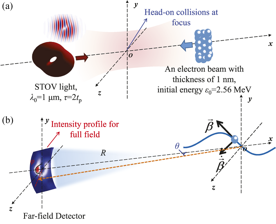


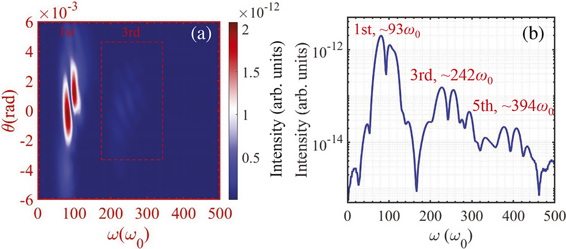


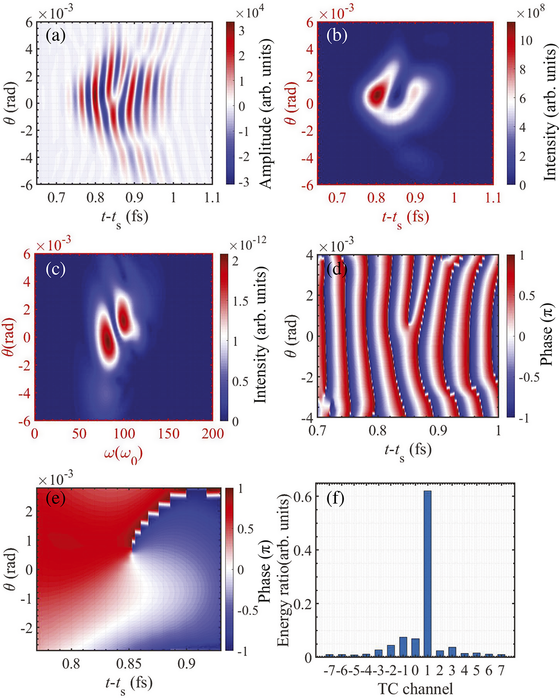


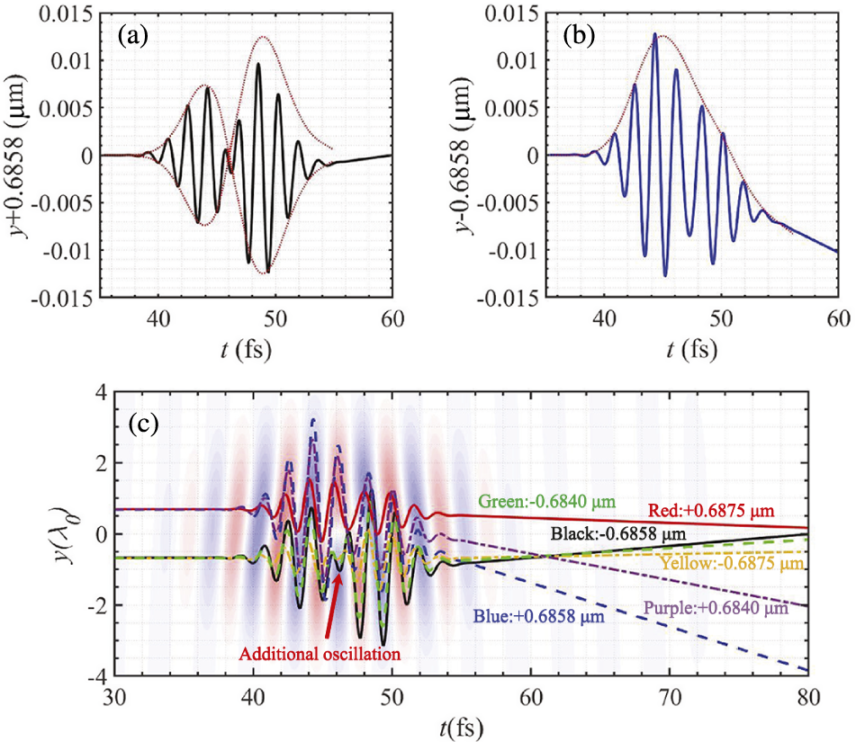


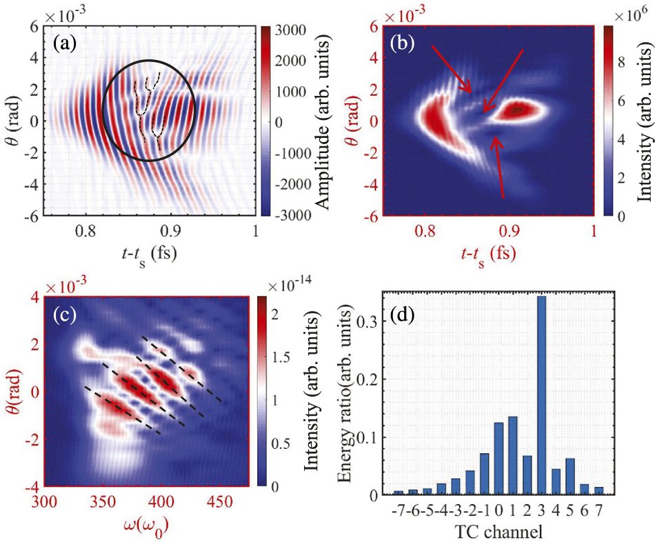
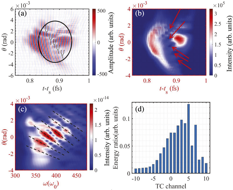
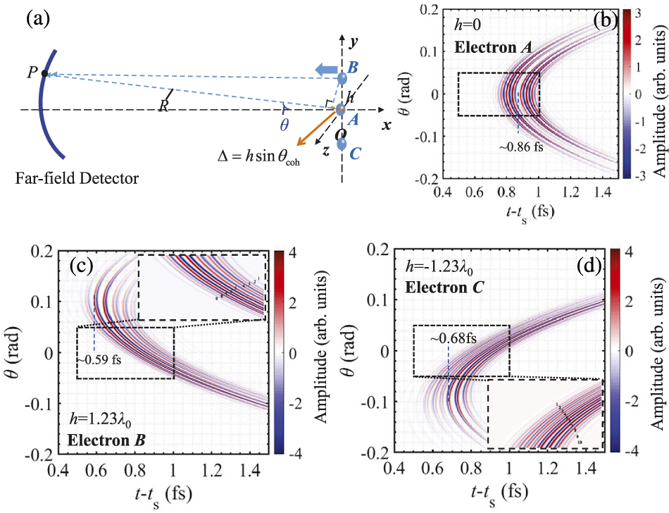


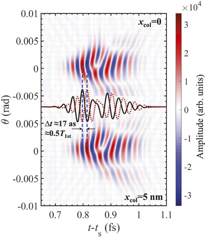


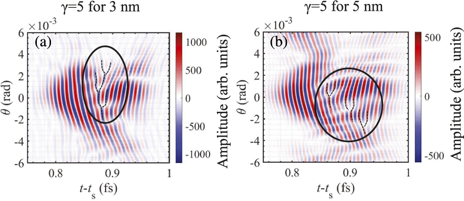
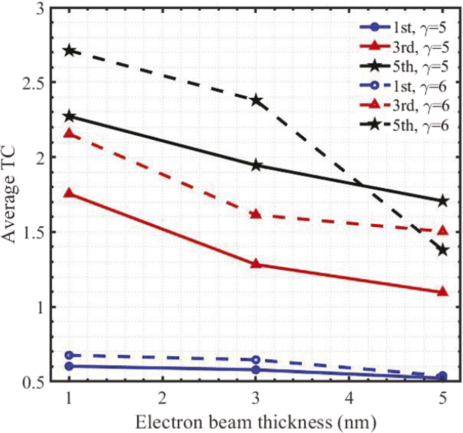


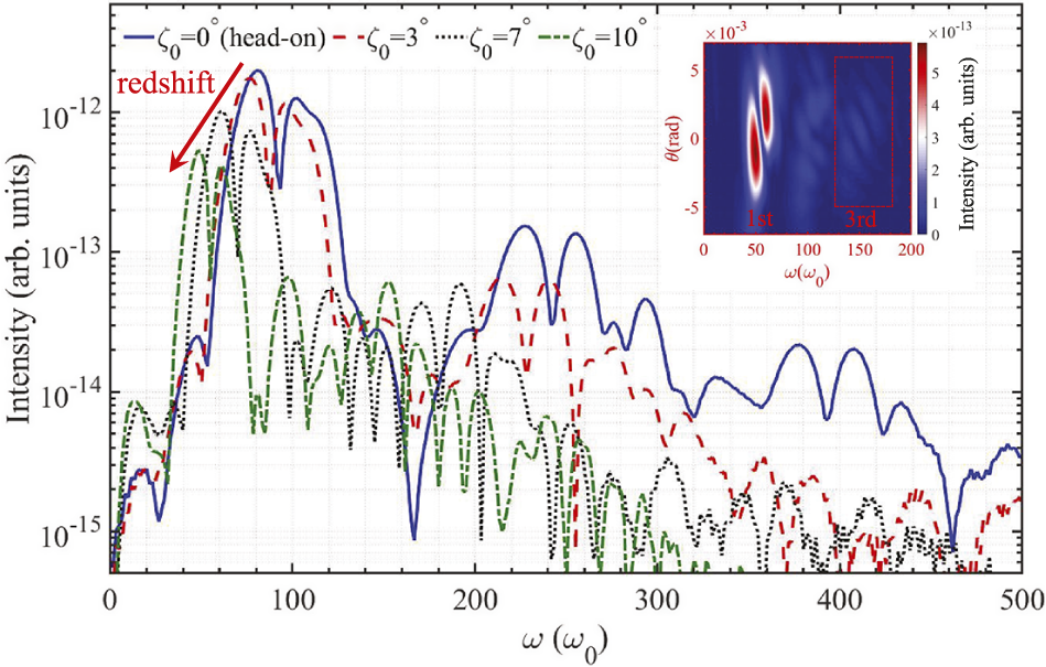


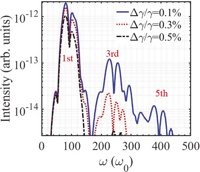


 Open access