


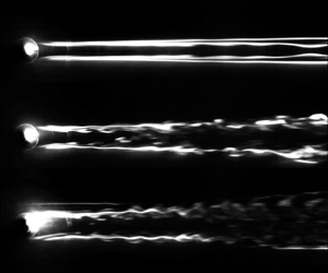





1. Introduction
The flow around an isolated roughness element is a fundamental problem in fluid mechanics that also appears in various engineering applications, such as on the surface of aircraft. Therefore, it has been a topic of research interest for many decades. A cylindrical roughness element can be defined by its diameter  $d$ and height $k$. The ratio of these two, $\eta =d/k$, is the roughness aspect ratio. To represent the influence of velocity in a non-dimensional manner, the roughness Reynolds number is generally introduced, $Re_{kk}=U_kk/\nu$. Here, $U_k$ is the mean velocity inside the undisturbed boundary layer at the roughness height $k$ and $\nu$ is the kinematic viscosity of the surrounding fluid. Note that in some works, the roughness Reynolds number is instead based on the free-stream velocity, denoted here as $Re_k=U_\infty \,k/\nu$. However, unless explicitly stated, we refer to $Re_{kk}$ as the roughness Reynolds number in this paper. It has been shown to adequately represent the fluid displacement effect due to the roughness (e.g. Tani Reference Tani1969; Puckert & Rist Reference Puckert and Rist2018).
As  $Re_{kk}$ increases, the modulated far-wake flow can become convectively unstable, with disturbances being amplified as they travel downstream. The onset of this instability will move upstream, closer to the roughness, with a further increase of $Re_{kk}$. At a critical value of $Re_{kk}$, the instability will switch to an absolute instability which takes place in the near-wake region and acts as a wavemaker. Studying the instabilities appearing in the close wake behind an isolated roughness element is an intricate stability problem since the flow cannot be considered parallel. However, as a result of increased computational capability and the advancement of numerical techniques, classical approaches using bi-local stability theory have been replaced by global linear stability analysis, which provides global instability modes for a given three-dimensional flow. This latter approach is today adopted by most researchers studying the instability behind roughness elements numerically. Additional well-performed experiments are essential at the current stage since direct comparisons with numerical works are feasible. For further advancements in this area, numerics and experiments must go hand in hand, both with their pros and cons. To give a full review of stability analysis and its historical advancement is beyond the scope of the present experimental paper; instead, interested readers unfamiliar with stability analyses are referred to the review works by Huerre & Monkewitz (Reference Huerre and Monkewitz1990), Chomaz (Reference Chomaz2005) and Theofilis (Reference Theofilis2011).
Early smoke-flow visualizations of three-dimensional roughness elements have been performed by Gregory & Walker (Reference Gregory and Walker1951), describing the generation and evolution of a horseshoe vortex that wraps around the cylinder. Mochizuki (Reference Mochizuki1961b) conducted visualizations on the wake of a spherical roughness, giving insight into the three-dimensional features of the flow and of the shed hairpin vortices. In the same year, they published results from hot-wire measurements (Mochizuki Reference Mochizuki1961a) in the wake of the spherical roughness element. In addition to confirming that the observations from smoke-flow visualizations indeed correlate well to fluctuations measured using hot-wires, they illustrate the existence of a high-speed streak in the centre of the wake. This can be attributed to the entrainment of high-momentum fluid from the free-stream due to the two counter-rotating legs of the horseshoe vortex. The opposite effect leads to two low-speed streaks neighbouring the high-speed streak. This effect is commonly observed given the Reynolds number of the flow is large enough, so that the horseshoe vortex can form. For lower Reynolds numbers, the wake effect of the isolated roughness predominates, featuring a low-speed streak in-line behind the roughness (cf. White, Rice & Ergin Reference White, Rice and Ergin2005).
Topologies of the flow behind various different shapes of roughness elements have been investigated by means of tomographic particle image velocimetry by Ye, Schrijer & Scarano (Reference Ye, Schrijer and Scarano2016), also with regards to accelerating the transition to turbulence. They state that the low-speed regions next to the central high-speed streak play a key role in the transition process as they cause inflectional velocity profiles. The onset of transition correlated well with the presence and extent of these secondary streaks for the different geometries. Similar reasoning was already proposed by Tani et al. (Reference Tani, Komoda, Komatsu and Iuchi1962), although their data were limited to cylindrical roughnesses. Furthermore, they point out the abruptness of arising turbulence by increasing the free-stream velocity compared to two-dimensional roughness elements, where the transition to turbulence is more gradual. More quantitative information, including comparison of various data sets, is given in the review paper by Tani (Reference Tani1969).
Data from a number of transition measurements on cylindrical roughnesses were compiled into a diagram plotting the roughness Reynolds number at which transition to turbulence occurs versus the roughness aspect ratio by von Doenhoff & Braslow (Reference von Doenhoff and Braslow1961), and this is still being used today as a reference. However, a significant amount of spread is present in this data set, which can be attributed to the previously mentioned abruptness of transition for this flow case and hence the sensitivity to small variations in the experiments. Klebanoff, Cleveland & Tidstrom (Reference Klebanoff, Cleveland and Tidstrom1992) performed transition measurements on hemispherical roughnesses and found that the effects are generally similar to cylindrical roughness elements, although absolute values of the onset of instability and transition differ.
It was demonstrated by Sakamoto & Arie (Reference Sakamoto and Arie1983) through smoke-flow visualizations that the flow structure behind an isolated roughness element can be either symmetric (varicose) or anti-symmetric (sinuous) with regard to the centreline. They performed experiments in a turbulent boundary layer and found that the aspect ratio of the element has a major influence on the structure of the wake. Note that they define the aspect ratio inversely to the definition used here, i.e.  $k/d$. Asai, Minagawa & Nishioka (Reference Asai, Minagawa and Nishioka2002) demonstrated experimentally that a streamwise streak tends to develop a sinuous instability if the width of the streak is narrow compared to the shear-layer thickness. Wider streaks are more likely to develop a varicose instability.
The role of transient growth in the transition to turbulence behind isolated roughness elements has been investigated both experimentally (e.g. White et al. Reference White, Rice and Ergin2005; Ergin & White Reference Ergin and White2006) and numerically (e.g. Denissen & White Reference Denissen and White2009, Reference Denissen and White2013). It was shown that this effect can cause substantial disturbance growth inside the boundary layer which can lead to the onset of secondary instabilities, even if no unstable mode is present. Moreover, Cherubini et al. (Reference Cherubini, De Tullio, De Palma and Pascazio2013) showed that transient growth can be significant, especially if  $k/\delta _1\geqslant 1$, where $\delta _1$ is the local displacement thickness of the undisturbed boundary layer at the roughness location. Bucci et al. (Reference Bucci, Puckert, Andriano, Loiseau, Cherubini, Robinet and Rist2018) suggested that the unsteadiness observed in the sub-critical regime is in fact not due to non-normality of the Navier–Stokes operator, but rather a result of quasi-resonance of the least stable varicose eigenmode with external excitations, such as free-stream turbulence. This was further investigated by Bucci et al. (Reference Bucci, Cherubini, Loiseau and Robinet2021). They showed that, depending on the frequency of the modes, different non-modal growth mechanisms are dominant. Phenomena such as harmonic forcing and localized wave packets (quasi-optimal perturbation) excited by free-stream turbulence can be important.
Employing a roughness element that is connected to a linear traverse so that the height can be varied, roughness-induced transition to turbulence and the interaction with Tollmien–Schlichting waves have been investigated by Hara, Mamidala & Fransson (Reference Hara, Mamidala and Fransson2022). Intuitively, a higher roughness tends to destabilize the boundary layer and to promote transition, also in the presence of imposed perturbations. However, contradictory to previous investigations, they show the presence of hysteresis in the transition Reynolds number by changing the roughness height at a constant free-stream velocity.
The dominant frequency in the roughness wake is expected to be critical for the transition process, as it represents the frequency of the most unstable mode. Visualizations of shed vortices behind a cylindrical roughness element in a water tunnel have been performed by Furuya & Miyata (Reference Furuya and Miyata1973), enabling the extraction of frequency information. Further experiments were performed by Klebanoff et al. (Reference Klebanoff, Cleveland and Tidstrom1992) for hemispherical roughnesses, giving a relation to predict the shedding frequency based on the free-stream velocity, the roughness height, the viscosity and the distance to the leading edge. More recently, Puckert & Rist (Reference Puckert and Rist2019) investigated the dominant frequencies in the wake of a cylindrical roughness element and were able to show the phenomenon of frequency lock-in between sinuous and varicose modes.
Fransson et al. (Reference Fransson, Brandt, Talamelli and Cossu2005) showed that the alternating high- and low-speed streaks generated by a spanwise array of cylindrical roughness elements can attenuate the growth of two-dimensional Tollmien–Schlichting waves in the boundary layer, revealing the potential to delay the transition to turbulence, which was proven by Fransson et al. (Reference Fransson, Talamelli, Brandt and Cossu2006). One case from the first study, alongside other cylinder dimensions, was reproduced numerically by Loiseau et al. (Reference Loiseau, Robinet, Cherubini and Leriche2014) by means of direct numerical simulation (DNS). From global stability analysis, they were able to determine a regime of global instability in the wake of the cylinder. Furthermore, they showed that for low aspect ratios ( $\eta =0.85$ and $\eta =1$), the globally unstable mode is of sinuous nature (anti-symmetric), while for higher aspect ratios ( $\eta =2$ and $\eta =3$), the global instability is varicose (symmetric). From their simulations, they were able to identify a critical Reynolds number where a global instability sets in. It was shown by Puckert & Rist (Reference Puckert and Rist2018), studying similar roughness aspect ratios but isolated elements, that the critical Reynolds number found by Loiseau et al. (Reference Loiseau, Robinet, Cherubini and Leriche2014) does not in fact represent the point where the transition to turbulence happens, but rather where the switch from convective to global instability takes place. They describe this value as an upper limit, at which transition happens the latest, but in many cases, the transition Reynolds number is lower than the critical Reynolds number. In these cases, transition is initiated by non-modal (transient) growth of globally stable eigenmodes. The results also show that the global instability characteristics behind the roughness do not change if an array or an isolated element is employed, given the elements are placed sufficiently far apart (here, $10 \times d$).
In the context of boundary layer tripping, the instability mechanism behind a cuboid roughness element featuring a square cross-section was investigated recently by Ma & Mahesh (Reference Ma and Mahesh2022) by means of global stability analysis and DNS. They found qualitatively similar results to Loiseau et al. (Reference Loiseau, Robinet, Cherubini and Leriche2014) for a cylindrical roughness, showing that the flow exhibits a sinuous global instability at low roughness aspect ratios and a varicose shape as the aspect ratio is increased. Absolute values differ, however, showing the two aforementioned instability shapes for values of  $\eta =0.5$ and $\eta =1$, respectively. The onset of global instability also appears to take place at lower Reynolds numbers, when compared to cylindrical roughness elements. Citro et al. (Reference Citro, Giannetti, Luchini and Auteri2015) performed global stability and sensitivity analysis of the wake of a hemispherical roughness element in a laminar boundary layer. They likewise demonstrated the existence of a global instability (wavemaker) close to the obstacle that leads to modal growth. In a parametric study, they showed that the critical Reynolds number decreases with increasing $k/\delta _1$. In all cases, the wake was dominated by symmetric (varicose) hairpin vortices.
The influence of free-stream turbulence in the inflow on the instabilities behind a cylindrical roughness element was investigated by Bucci et al. (Reference Bucci, Cherubini, Loiseau and Robinet2021). Using the skin-friction coefficient as a measure, they concluded that a significant increase is observed already at turbulence intensities in the range of 0.06–0.09 % when compared to cases without any free-stream disturbances. They also state that the integral length scale of the incoming turbulence has a negligible influence at these low values of turbulence intensity. Furthermore, they illustrate that the quantity  $k/\delta _1$, in addition to $Re_{kk}$ and $\eta$, has an influence on the nature of the instability that develops behind the roughness.
The present experimental investigation aims to give a more complete picture on the prevailing instability mechanism behind a roughness element. For this, smoke-flow visualization in the wake of an isolated cylindrical roughness is employed and methods to distinguish instability mechanisms are discussed. Furthermore, techniques to extract quantitative information (such as dominant frequencies) from the results are explored. The used roughness element is connected to a linear motor, enabling continuous height variation in a range of more than 10 mm, similar to the set-up in the experiments by Hara et al. (Reference Hara, Mamidala and Fransson2022). In total, we are reporting 88 different roughness cases.
The paper begins with a short overview of the experimental set-up, including the smoke-flow visualization technique and the traversable roughness element in § 2. In § 3, we present employed methods to discriminate between the different instability mechanisms and provide an instability map, showing the type of instability for a large number of investigated cases. Furthermore, frequency information from the time-resolved images is extracted in an attempt to give a generalized non-dimensional representation. Finally, in § 4, we summarize our results.
2. Experimental set-up
2.1. Wind tunnel set-up
Experiments were performed in the MTL (Minimum Turbulence Level) wind tunnel at KTH Royal Institute of Technology. The test section of the closed-loop tunnel has a length of 7 m and a cross-sectional area of  $1.2\,\mathrm {m} \times 0.8\ {\rm m}$ ( ${\rm width} \times {\rm height}$). The maximum speed inside an empty test section is $69\ {\rm m}\ {\rm s}^{-1}$ and the turbulence intensity at the nominal speed of $25\ {\rm m}\ {\rm s}^{-1}$ is less than 0.025 %. Free-stream velocities in the present study were set in a range of $U_\infty =1\unicode{x2013}4\ {\rm m}\ {\rm s}^{-1}$. The temperature controller was not used due to the very low wind-tunnel speeds. However, the air temperature in the test section was monitored and remained within a range of less than $0.5\,^\circ {\rm C}$.
The experimental set-up consisted of a flat plate with an asymmetric leading edge (cf. Westin et al. Reference Westin, Boiko, Klingmann, Kozlov and Alfredsson1994) and a trailing edge flap that was adjusted to tune the location of the stagnation line on the leading edge. The ceiling was adjusted to minimize the streamwise pressure gradient and to create a boundary layer in agreement with the Blasius solution.
Various cylindrical roughness elements with four different diameters (3 mm, 6 mm, 12 mm and 24 mm) were stationed at a streamwise location of 450 mm from the leading edge of the plate. The elements were connected to an OptoSigma RMH-13 linear motor which has a precision of  $1\ \mathrm {\mu }{\rm m}$ and allows continuous height adjustment of the roughness element in the range of 0 to 13 mm.
2.2. Smoke-flow visualization set-up
Measurements by means of smoke-flow visualization were performed in this study. The smoke was generated by a JEM ZR25 fog machine and collected in an intermediate tank with a volume of approximately 75 l. Using hoses, the tank was connected to a small spanwise cavity within the flat plate with a narrow spanwise slot to the plate surface 210 mm downstream of the leading edge to inject a homogeneous smoke sheet into the boundary layer. Between the tank and the cavity, DC fans were used to provide a steady smoke flux. It could be seen by the naked eye that providing an excessive voltage to the fans caused instability or even premature transition due to the wall-normal jet. In all measurements, it was ensured that no visual perturbations in the smoke sheet were present by keeping the supply voltage to the fans as low as possible. The smoke was illuminated using a thin laser sheet positioned a few millimetres from the wall. The employed laser was a continuous wave (CW) laser with a wavelength of 532 nm and a power of up to 1.5 W.
Smoke images were recorded using three synchronized MotionBLITZ EoSens mini1 high-speed cameras equipped with 50 mm lenses. They were mounted outside the wind tunnel from a top view and the individual fields of view had an overlapping area of approximately 25 mm. The cameras had a resolution of  $1280\times 1024$ pixels and a maximum frame rate of 506 frames per second (fps) at this image size. For the present experiments, the full resolution and a frame rate of 200 fps were used. This resulted in a time series of 1636 images, corresponding to 8.18 s of real-time acquisition. In all measurements, it was ascertained that a steady state in the flow was reached before starting the recording. For the final merged image, overlapping regions were averaged using a weighted mean of the two images, based on the distance to the image edge. The combined field of view covered an area of roughly $650\times 190$ mm, starting at approximately 400 mm from the leading edge and the resolution of the final images/videos was $3592\times 922$ pixels. A sketch of the experimental set-up is shown in figure 1.
Schematic of the experimental set-up. All dimensions are in millimetres.

2.3. Hot-wire anemometry
Boundary-layer velocity profiles were measured by means of hot-wire anemometry. The probes were manufactured in-house and had a wire length of 0.5 mm and a diameter of  $2.5\ \mathrm {\mu }{\rm m}$. They were calibrated inside the wind tunnel against a Prandtl tube connected to a Furness FCO560 differential manometer. The hot-wire data were collected using a 16-bit, NI USB-6215 DAQ system with a sampling frequency of 10 kHz and a sampling time of 10 s. The time series was high-pass filtered with a cutoff frequency $f_{hp}$ based on the free-stream velocity according to the following relation: $f_{hp}=U_\infty /L_{ref}$, where the reference length is $L_{ref}=2$ m. This is (with some margin) the largest possible cross-sectional length scale in the flow, based on dimensions of the wind tunnel test section ( ${\rm height} + {\rm width}$).
3. Results
3.1. Base flow
As a first step, the velocity profile at the roughness location (450 mm from the leading edge) was measured at different velocities using hot-wire anemometry. Free-stream velocities for the performed smoke-flow visualizations were in the range of  $1\unicode{x2013}4\ {\rm m}\ {\rm s}^{-1}$ and boundary layer profiles were measured at these velocities. Results are shown in figure 2(a). The agreement with the Blasius solution is good and confirms that the streamwise pressure gradient is close to zero. Note that hot-wire anemometry is not ideal for measuring low speeds below $1\ {\rm m}\ {\rm s}^{-1}$ and close to the wall due to natural convection from the heated wire as well as heating of the wall, hence several points near the wall were discarded. In the following, the velocity inside the boundary layer at the roughness height ( $U_k$), and hence quantities such as $Re_{kk}$, are determined from the theoretical Blasius solution based on $U_\infty$ at the roughness location. Furthermore, figure 2(b) shows the fluctuation level inside the boundary layer, plotting the normalized root mean square (r.m.s.) of the velocity signal. The turbulence intensity increases slightly towards lower free-stream velocities but, overall, features very low values below 0.03 % throughout the whole boundary layer. This fluctuation level is well below the values where Bucci et al. (Reference Bucci, Cherubini, Loiseau and Robinet2021) reported a significant change in the skin-friction coefficient.
(a) Mean boundary layer profiles at the roughness location for different free-stream velocities compared to the Blasius solution. (b) Fluctuation velocity profiles in the boundary layer. Here,  $\delta _1$ is the displacement thickness of the boundary layer.

3.2. Varicose versus sinuous instability
In the context of fluid mechanics, a streamwise velocity streak can become unstable either in a varicose or a sinuous manner. While the varicose instability is symmetric with regards to the centreline, the sinuous mode is anti-symmetric. Likewise, the dominant disturbance in the wake of a roughness element will develop to either of those two instability modes, unless the wake instability is bypassed altogether, causing immediate breakdown to turbulence, or remains fully stable (e.g. Andersson et al. Reference Andersson, Brandt, Bottaro and Henningson2001). One straightforward way to distinguish the instability mode from smoke-flow visualizations is to perform a visual inspection of the images one-by-one. This gives a clear result in most cases, however, proper orthogonal decomposition (POD) can be applied to the time series of images to confirm this observation in an objective manner. As an example, a varicose instability is illustrated in figure 3 and its corresponding first four POD modes are shown in figure 4. The first POD mode appears to be present due to variations in smoke density over time, but all other modes clearly show varicose disturbance patterns.


Likewise, a sinuous mode is displayed in figure 5 and its POD modes in figure 6. From both the raw smoke-flow visualization and the POD modes, it becomes clear that the dominant mode is sinuous for these conditions. It should be noted that in many cases, in which a dominant sinuous mode was detected, the breakdown to turbulence appears to be a varicose event, as can be seen in modes 3 and 4 in figure 6. The coexistence of varicose and sinuous modes in the wake of the roughness has been observed before, especially if the leading instability shape is sinuous, e.g. Bucci et al. (Reference Bucci, Puckert, Andriano, Loiseau, Cherubini, Robinet and Rist2018) and Ma & Mahesh (Reference Ma and Mahesh2022).


3.3. Global versus convective instability
In addition to the classification depending on the shape of the coherent structures in the wake, the instability regime behind a cylindrical roughness element can be divided into a sub-critical and a super-critical regime (e.g. Loiseau et al. Reference Loiseau, Robinet, Cherubini and Leriche2014; Puckert & Rist Reference Puckert and Rist2018). Note that, in general, a streak can exhibit any combination of sinuous/varicose and sub-/super-critical conditions. In the scope of this publication, the term ‘critical’ refers to the boundary between these two instability regimes, in accordance with Puckert & Rist (Reference Puckert and Rist2018), rather than the point where the transition to turbulence occurs.
In the sub-critical regime (convective instability), the roughness acts as an amplifier, intensifying any incoming disturbances in the flow. The behaviour is intermittent as it relies on randomly occurring perturbations in the boundary layer. The flow must extract energy from external perturbations to become unstable, transporting kinetic energy from the free-stream disturbances to the vicinity of the element and causing destabilization when a certain threshold is overcome as a result of non-modal (transient) growth. Global stability analysis, as performed e.g. by Bucci et al. (Reference Bucci, Puckert, Andriano, Loiseau, Cherubini, Robinet and Rist2018, Reference Bucci, Cherubini, Loiseau and Robinet2021), reveals a branch of stable eigenmodes that are susceptible to transient growth in the case of sufficiently strong incoming perturbations. However, in the super-critical regime (global instability), the role of the roughness is that of a wavemaker. This requires the existence of an unstable eigenmode, where self-sustained instabilities in the wake are induced through modal growth, regardless of incoming disturbances. In this case, the instability is continuous as it does not depend on randomly occurring events.
In the experiments by Puckert & Rist (Reference Puckert and Rist2018), this distinction was made based on hot-film signals acquired in the roughness wake. The signal was bandpass filtered around the natural instability frequency and the envelope of this signal was determined. As per the previously described difference between the two instability mechanisms (transient or continuous), the envelope in the sub-critical regime exhibited a significantly higher standard deviation (STD) value compared to the super-critical regime. Note that the STD is equal to the r.m.s. of the signal after subtracting its mean. Hence, the Reynolds number where this sudden drop arises was identified as the transition point between the two instabilities, referred to as critical Reynolds number  $Re_{kk,crit}$.
Similar results can be drawn from the performed flow visualizations. By observing the time behaviour of a carefully chosen pixel in the wake of the cylinder, it is possible to identify the instability mechanism (figure 7). The selected pixel has to be on the inner edge of the smoke line where a significant fluctuation in brightness with time is present. Due to the relatively low sampling frequency of 200 frames per second, it is hardly possible to low-pass filter the time series. However, a moving mean of the signal was computed and subtracted from the time series to remove fluctuations due to changes in smoke density, which effectively acts as a high-pass filter. Additionally, each signal was normalized by its standard deviation to minimize the effect of varying smoke conditions during different runs. Results show a clear distinction between convective and global instability, especially in the shape of the envelope.
Showcase timelines of the brightness of a selected pixel for (a) convective and (b) global instability behind the roughness element. Note the difference in scale of the ordinate axes in (a,b). Cases are indicated in figure 8.

The STDs of the envelopes for two different conditions with a variation of cylinder height are shown in figure 8. Note that within one combination of free-stream velocity and cylinder diameter (i.e. one line in figure 8), the chosen pixel was kept constant for all roughness heights. Results are presented for a cylinder diameter of 6 mm at two different free-stream velocities ( $2.4\ {\rm m}\, {\rm s}^{-1}$ and $2\ {\rm m}\ {\rm s}^{-1}$) and $Re_{kk}$ is raised by increasing the roughness element height in small steps in a range of 4–11 mm. More detailed information is provided in table 1, Cases R1 and R2. In all cases, the lower envelope of the signal turned out to give more reliable results than the upper envelope. This is likely due to the lower limit of the signal (completely black), whereas the upper envelope is affected by the randomly varying smoke density that affects the momentary pixel brightness. Similar to the hot-film measurements by Puckert & Rist (Reference Puckert and Rist2018), a clear drop in the envelope STD can be observed, where the transition from convective to global instability takes place. Additionally, the $2\ {\rm m}\ {\rm s}^{-1}$ case shows a drop at $Re_{kk}\approx 790$ and then a sudden rise at $Re_{kk}\approx 1030$, indicating that a further increase in height leads to a return to a convective instability. This case will be discussed in more detail in the subsequent section.
Standard deviation of the envelopes of pixel brightness with increasing  $Re_{kk}$ by raising the roughness element. Parameter ranges are given in table 1, Cases R1 and R2. Red circles indicate cases shown in figure 7. Low STD values (<0.2) represent a global instability while high values ( ${\approx }1$) mark a convective instability.

Detailed description of some selected cases indicated in figure 10. Cases C1–C7 are discussed in the text, R1 and R2 are roughness height ranges indicated in figure 8. A flow visualization video corresponding to each of these cases can be found in the supplementary movies available at https://doi.org/10.1017/jfm.2023.171.

Although the general shape of the envelope STD evolution is similar, the amount of the sharp drop can strongly depend on the selected pixel. Hence, another way to discriminate between global and convective instability is to visually inspect the smoke-flow visualization video frame-by-frame. A clear distinction can be seen between a convective instability, where transient wave trains pass through the wake followed by time windows of no apparent instability, while for a global instability, the fluctuation is continuously present. In general, the conclusions drawn from these methods are in good agreement.
Another distinction is that the global instability tends to be visible right behind the roughness element, which is the main counterflow region and thus the location of the wavemaker, leading to modal (exponential) growth. For the convective instability, however, in most cases, the disturbances appear further downstream and are caused by external disturbances with a minimal amplitude. These perturbations can excite otherwise stable modes, having the strength to overcome dissipation and to distort the base flow through non-modal growth, which is of polynomial order (and therefore generally slower than modal growth). The exact location where this distortion becomes visible is expected to depend on the free-stream turbulence intensity. In the current experiments, the turbulence intensity is low enough (cf. figure 2b), so that the modal growth of the unstable self-sustaining mode can compete with transient growth of the convective instability. This distinction between the different growth mechanisms is clearly seen in the previously shown figures 3 and 5 for a convective and a global instability, respectively. For comparison, a globally unstable varicose case is shown in figure 9.

3.4. Instability map
The methods outlined in the previous sections were used on a large number of flow visualization cases to generate an instability diagram in the  $Re_{kk}\unicode{x2013}\eta$ space (figure 10). The marker shape represents the diameter of the roughness: diamond, circle, square and triangle correspond to 3 mm, 6 mm, 12 mm and 24 mm, respectively. The colour of the marker represents the type of instability. Black indicates that no periodic movement of the wake can be seen by the naked eye, red indicates a clear varicose movement of the smoke streaks and blue represents a sinuous instability. The green points (Cases C6 and C7) show a mixture of both shapes and will be discussed in more detail. Finally, global instabilities are shown with a filled symbol while convective instabilities have open symbols.
Instability map of the wake of a cylindrical roughness element in the  $Re_{kk}\unicode{x2013}\eta$ space. Colours display instability shape: black, no visible instability; red, varicose; blue, sinuous. Open symbols represent convective, filled symbols global instabilities. Markers show roughness diameter: $\blacklozenge$, 3 mm; $\bullet$, 6 mm; $\blacksquare$, 12 mm; $\blacktriangle$, 24 mm. Numbered cases are listed in tables 1 and 2. R1 and R2 represent the parameter ranges when changing only the roughness height, as indicated by the grey lines. All the data are provided in table 3.

The two grey lines indicated as R1 and R2 represent the ranges of roughness height variation presented in figure 8. It becomes clear that in the present set-up with a traversable roughness, a change in roughness height  $k$ causes both $Re_{kk}$ and $\eta$ to vary simultaneously (at a constant $U_\infty$). It was not attempted here to modify either of them in an isolated manner, which would be possible by adjusting the free-stream velocity for each roughness height. The dashed lines at low $\eta$ and low $Re_{kk}$ indicate further regions where no instability was seen by eye. Each line represents a case with a constant roughness diameter and free-stream velocity while the height is varied successively. Likewise, the grey dotted lines represent a regime where the flow appears fully turbulent right behind the roughness and a clear instability mode is difficult to identify. Note that the boundaries where either of these regimes begin are subjective and the lines only serve as a qualitative trend.
As a first observation, the shapes of the instabilities agree well with results from the literature. The global instability in an aspect ratio range of  $0.7\leqslant \eta \leqslant 1.2$ is of sinuous nature, while it is varicose for $\eta \geqslant 2$. In the sub-critical regime (i.e. at lower roughness Reynolds numbers, $Re_{kk}\lesssim 750$), the disturbance pattern is strictly varicose for all aspect ratios. Similar effects were shown by Puckert & Rist (Reference Puckert and Rist2018) at $\eta =1$. By increasing the free-stream velocity gradually to increase $Re_{kk}$, they showed a switch from varicose convective to sinuous global instability at the critical point. These findings agree with the results of Loiseau et al. (Reference Loiseau, Robinet, Cherubini and Leriche2014), stating that in this range of $\eta \approx 1$, all modes are varicose except for one isolated sinuous mode that becomes globally unstable at the critical Reynolds number. Below that, transient growth of the stable varicose modes causes the observed instability. In agreement with this, it was also found by Cherubini et al. (Reference Cherubini, De Tullio, De Palma and Pascazio2013) that the varicose modes experience the strongest transient growth. This goes along with the observation that there are no convective instabilities of sinuous nature in any case investigated here. Bucci et al. (Reference Bucci, Cherubini, Loiseau and Robinet2021) came to a similar result. They investigated a globally stable case, where the eigenmode with the largest growth rate (marginally stable) features a sinuous shape. By forcing this type of flow with very weak free-stream turbulence, they found that the disturbance pattern in the wake is still varicose, showing that the free-stream disturbances always amplify the varicose modes. They explain this observation by stating that there is only one single sinuous mode and a continuous branch of varicose eigenmodes in the spectrum. The sinuous mode can be excited through forcing at that specific frequency, but broadband free-stream turbulence will always favour the branch of varicose eigenmodes.
Further effects are observed at particularly low aspect ratios ( $\eta <0.7$). Here, no global instability can be identified so that varicose convective instabilities are predominant even at the highest tested $Re_{kk}$. As the smallest $\eta$ investigated by both Loiseau et al. (Reference Loiseau, Robinet, Cherubini and Leriche2014) and Puckert & Rist (Reference Puckert and Rist2018) was 0.85, no firm conclusion regarding global instabilities can be drawn for this range, but the data suggest that no globally unstable regime exists for this range of aspect ratios. This gives rise to an interesting phenomenon, since $\eta$ and $Re_{kk}$ are coupled through $k$. When increasing the roughness height gradually, it is possible that one moves from globally stable to unstable and then, at an even larger height (i.e. at a lower $\eta$), the flow becomes globally stable again. One range of parameters where this sequence of instabilities can be observed was mentioned earlier in figure 8 and is indicated as R2 in figure 10 and in table 1. This observation is consistent with the re-stabilization of the leading eigenmode shown by Loiseau et al. (Reference Loiseau, Robinet, Cherubini and Leriche2014).
In contrast, in the investigation by Ma & Mahesh (Reference Ma and Mahesh2022), employing a roughness element with a square cross-section, a (sinuous) global instability was identified for an aspect ratio of  $\eta =0.5$. It could be that, due to the curved streamlines, the flow around the cuboid roughness has similar features to the flow around a circular roughness of slightly larger diameter, implying comparable effects but with an offset in absolute values between different roughness shapes.
Figure 10 indicates the general trend that the  $Re_{kk}$, where the onset of instability (of varicose convective type) takes place, decreases with increasing $\eta$. However, towards very high aspect ratios, the roughness Reynolds number at which the first instabilities become visible appears to increase, suggesting a more stable flow. At $\eta =6.9$ and $Re_{kk}=476$, no instability can be detected by eye (figure 11a). A cylindrical roughness with a smaller diameter (12 mm instead of 24 mm, featuring $\eta =4.84$), shows a clear convective instability behind the roughness at even lower $Re_{kk}=313$ (figure 11b). More detailed information on these two cases is given in table 1, Cases C4 and C5, respectively. Note that the case in between the two described ones at $(\eta,Re_{kk})=(5.45,302)$ shows a less pronounced, but still clearly visible varicose instability. No quantitative conclusions regarding the transition to turbulence can be drawn with the current method, but it appears as if the larger cylinder is less prone to induce transition compared to the smaller diameter. Following the whole time-series of images, although rarely, the formation of turbulent spots can be observed in the case of the smaller roughness (Case C5), while the larger roughness (Case C4) shows no perturbation. This, at first thought, is counter-intuitive as the blockage due to the roughness increases. A possible explanation is that the larger cylinder induces larger streaks with more independent dynamics compared to the smaller one. The large streak might be stable for longer but then abruptly destabilizes, making it more difficult to observe the linear amplification phases. For small elements, however, the transitions are more subtle and happen progressively, allowing the observation of intermediary phases. Furthermore, the secondary (i.e. streak) instabilities are inviscid and caused by strong wall-normal (varicose) and spanwise (sinuous) mean velocity gradients of the primary wake flow disturbance (cf. Andersson et al. Reference Andersson, Brandt, Bottaro and Henningson2001). For larger streaks, the spatial velocity gradients will generally be lower, alleviating the growth of secondary instabilities. However, a more detailed analysis of the base flow is needed to explain the observed trend profoundly. Note that the same tendency is not visible in the transition diagram by von Doenhoff & Braslow (Reference von Doenhoff and Braslow1961), but it could also be a result of the large spread of the data. This is likely related to variations in parameters in the different experimental campaigns, such as free-stream turbulence intensity, the streamwise pressure gradient and possibly more that affect the transition to turbulence.
Snapshots of two different flow visualization cases: (a)  $d=24$ mm, $k=3.5$ mm, $U_\infty =2.9\ {\rm m}\ {\rm s}^{-1}$ and (b) $d=12$ mm, $k=2.9$ mm, $U_\infty =3.4\ {\rm m}\ {\rm s}^{-1}$. The wake of the larger roughness does not show perturbations, while the smaller diameter is unstable at an even lower Reynolds number. Cases C4 and C5 in table 1, respectively.

One noteworthy case in the  $Re_{kk}\unicode{x2013}\eta$ map is presented in figure 12. It shows a roughness diameter of $d=3$ mm, free-stream velocity of $U_\infty =3.4\ {\rm m}\ {\rm s}^{-1}$ and a height of $k=4.2$ mm (Case C6 in table 1). From figure 10, it can be deduced that this point is in the bottom-left corner of the sinuous global instability region in the $Re_{kk}\unicode{x2013}\eta$ diagram. What makes this case particular is that in the vicinity of the roughness element, this global instability of sinuous type is present, although weak. Instead of growing, it seems to die out with the downstream distance, as can also be seen in the POD plot (figure 12b). Then, even further downstream (indicated by the red ellipse), a weak convective varicose instability sets in. Note that this event is too rare to be picked up by the POD technique when applied to that region. A possible explanation for this phenomenon can be found in results by Loiseau et al. (Reference Loiseau, Robinet, Cherubini and Leriche2014). They show that the region of global instability in the wake (wavemaker) is finite and gets shorter with decreasing aspect ratio $\eta$ ( $x/d\approx 75$ for $\eta =1$ and $x/d\approx 50$ for $\eta =0.85$). It can be expected that if the exponential growth region is passed without major nonlinearity, the flow returns back to an undisturbed state. Here, the wake again has the properties of an amplifier, i.e. intermittent varicose disturbances appear due to non-modal growth of globally stable modes, as described earlier. Two other cases where a qualitatively similar behaviour can be observed are located right above the described Case C6 in the $Re_{kk}\unicode{x2013}\eta$ diagram. Both feature a diameter of $d=6$ mm and therefore show overall stronger perturbations in the wake compared to $d=3$ mm, indicating that the flow is no longer fully laminar in the far wake. A video of one of these cases including detailed information of the parameters is provided in the supplementary movies (Case C6 $b$).
$b$).
(a) Snapshot of a case showing a global sinuous instability in the near wake (yellow rectangle) and a convective varicose instability further downstream (red ellipse). (b) One of the two POD modes featuring the global instability, obtained in the yellow frame. Case C6 in table 1.

Another interesting case is illustrated by two different snapshots of the same video in figure 13. This case (Case C7 in table 1) is located right on the edge where the transition back from global sinuous to convective varicose instability due to a decrease in aspect ratio (and increase in  $Re_{kk}$) occurs. Here, the modes can be seen to switch back-and-forth with time, even though all conditions ( $U_\infty$, $k$ and $d$) are kept constant. This indicates that there is no significant hysteresis present when switching modes at this point. A physical explanation of this effect could be that at these conditions, the modal and non-modal growth mechanisms exhibit very similar amplification magnitudes. Hence, the momentarily dominating mode depends on randomly appearing disturbances in the in-flow, featuring a varicose shape when non-modal growth is stronger and sinuous, when the modal growth prevails. These findings coincide with results from Bucci et al. (Reference Bucci, Puckert, Andriano, Loiseau, Cherubini, Robinet and Rist2018). Varying the Reynolds number at a constant aspect ratio of $\eta =1$, they showed the prevalence of the sinuous mode, but also the existence of the stable varicose mode. The latter could be triggered extremely easily, even by residuals of the turbulence intensity, leading to a non-modal growth of the instability due to the combination of stable convective eigenmodes.
Snapshots of (a) varicose and (b) sinuous instability in the same case, switching back-and-forth with time. Here,  $d=6$ mm, $k=8.1$ mm, $U_\infty =2\ {\rm m}\ {\rm s}^{-1}$. Case C7 in table 1.

Table 1 provides more detailed information for the previously discussed cases. Additional cases are added in table 2, which show the critical conditions, i.e. where the change from convective to global instability occurs (CR, critical). Data are shown for low aspect ratios where the transition is well resolved by the current experiments and all quantities of the last stable and first unstable data point are averaged. This allows to extract critical Reynolds numbers, enabling comparison to values from Loiseau et al. (Reference Loiseau, Robinet, Cherubini and Leriche2014) and Puckert & Rist (Reference Puckert and Rist2018). Note that Puckert & Rist (Reference Puckert and Rist2018) explicitly reproduced the cases studied by Loiseau et al. (Reference Loiseau, Robinet, Cherubini and Leriche2014) and hence observed very good agreement in critical Reynolds number. In the current experiments, the height of the roughness with respect to the local boundary layer ( $k/\delta _1$) was not attempted to match the aforementioned cases and thus some deviation can be expected.
Comparison of critical conditions (CR1 and CR2 in figure 10) with values reported by Puckert & Rist (Reference Puckert and Rist2018) (P&R).

The juxtaposition (table 2) reveals opposite trends, depending on the definition of the Reynolds number. For the case of  $\eta =1$ (current experiments: CR2, $\eta =1.04$), we find a higher $Re_{kk,crit}$, compared to the value reported by Puckert & Rist (Reference Puckert and Rist2018), proposing more stable flow conditions. However, $Re_{k,crit}$ has a lower value than that found by them for the same case, indicating a more unstable behaviour. Comparing the $\eta =0.85$ case from Puckert & Rist (Reference Puckert and Rist2018) with CR1 ( $\eta =0.92$), a similar trend can be observed. Remember that for $Re_{kk}$, the reference velocity is the velocity inside the undisturbed boundary layer at the roughness height $U_k$, while $Re_{k}$ uses the free-stream velocity $U_\infty$ as reference. In a Blasius boundary layer, those two velocities scale almost linearly for ratios of $k/\delta _1\lesssim 1$. However, this ratio deviates notably between the compared cases and so the observed effect can be attributed to this.
As mentioned before, we expect the parameter  $Re_{kk}$ to be superior to $Re_{k}$ in its ability to capture the combined effects of roughness height and velocity, in accordance with many other researchers (e.g. Tani Reference Tani1969; Puckert & Rist Reference Puckert and Rist2018). It could be argued that $U_\infty$ has a minor effect as the roughness element does not directly experience this velocity, in contrast to $U_k$. Hence, it appears that an increase in $k/\delta _1$ raises the critical Reynolds number, showing a stabilizing effect. Employing a stability diagram that plots $Re_{kk}$ against $k/\delta _1$ at a constant $\eta =1$, Bucci et al. (Reference Bucci, Cherubini, Loiseau and Robinet2021) come to similar conclusions.
The parameter  $k/\delta _1$ can be interpreted as the third axis in the previously presented instability diagram in figure 10. The isolated effect of this quantity on the type of the instability at a constant aspect ratio $\eta$ is investigated in figure 14. Although $\eta$ is constantly changing in the current campaign, cases within in a narrow range around $\eta =1$ are considered. The previously mentioned data points by Bucci et al. (Reference Bucci, Cherubini, Loiseau and Robinet2021) (figure 4 in their paper) are also added to the figure and plotted as hexagram symbols. As $k/\delta _1$ was not the primary variable in the current set of experiments, our data points lie almost on a straight line and are clearly correlated. The data show convective varicose instabilities (sub-critical behaviour) for low values of $k/\delta _1$ and then a transition towards sinuous global instabilities (super-critical) as both $k/\delta _1$ and $Re_{kk}$ are increased. However, the exact line of transition from sub- to super-critical is not as clear. Results from Bucci et al. (Reference Bucci, Cherubini, Loiseau and Robinet2021) indicate an almost horizontal line ( $Re_{kk}\approx 800$) at $k/\delta _1=2$ that separates the two regimes. In the present data, the globally unstable point $k/\delta _1=2.06$ features a lower $Re_{kk}=788$ than the stable point $k/\delta _1=1.99$ ( $Re_{kk}=832$). Note that both data points have a slightly smaller aspect ratio of $\eta =0.91$ and $\eta =0.94$, respectively, which might also influence the results. Regardless, a newly proposed separation line is drawn in figure 14.
Instability diagram showing  $Re_{kk}$ against $k/\delta _1$ for an almost constant aspect ratio of $\eta \approx 1$. Colours and symbols are similar to figure 10. Opaque points correspond to $0.9<\eta <1.1$, otherwise $0.95<\eta <1.05$. Hexagram symbols indicate data from Bucci et al. (Reference Bucci, Cherubini, Loiseau and Robinet2021, Reference Bucci, Puckert, Andriano, Loiseau, Cherubini, Robinet and Rist2018) and Loiseau et al. (Reference Loiseau, Robinet, Cherubini and Leriche2014). The dashed line shows the critical conditions, where the transition from convective varicose to global sinuous instability takes place.

3.5. Frequency analysis
In this section, the dominant frequency of the instability in the cylinder wake is investigated. As mentioned before, all images were sampled at a rate of  $f_s=200$ Hz. In some cases (especially at lower roughness diameters), this relatively low sampling frequency caused obvious aliasing of the data, e.g. structures appearing to move upstream. These cases are regarded with special attention in the following.
For the frequency analysis of the recorded image series, the image size was reduced by a factor of 2 in each dimension and afterwards, a Fourier transform in time for each individual pixel was performed. Zero-padding was used to improve the frequency resolution of the spectrum. As a result, a dominant frequency as a function of space was determined by identifying the maximum of each spectrum. To reduce the computing time, this procedure was only executed on pixels that had a standard deviation value above a fixed threshold. Results are displayed for a global and a convective instability in figures 15 and 16, respectively. In the next step, a histogram of pixel values is generated for each frequency analysis figure, as shown in figure 17. As can already be deduced from figures 15(b) and 16(b), results differ strongly between the global and convective instability regimes.
Frequency analysis of sinuous global instability: (a) snapshot of smoke-flow visualization and (b) dominant frequency for each individual pixel.

Frequency analysis of varicose convective instability: (a) snapshot of smoke-flow visualization and (b) dominant frequency for each individual pixel.

Histograms of pixel count for (a) global and (b) convective stability. Data correspond to figures 15(b) and 16(b), respectively.

The method gives unambiguous results in the case of a global instability, where the wake flow is dominated by one fixed frequency, which is that of the globally unstable mode. For the showcase in figures 15 and 17(a), a clear dominant frequency around 56 Hz can be identified. A second, lower maximum in the spectrum of 88 Hz is also present, which is the alias of the first harmonic (112 Hz) that can be expected here as per the Nyquist frequency of  $f_{Ny}=100$ Hz. As the streaks break down to turbulence in the far wake, a clear peak frequency can no longer be detected. For convective instabilities, however, results are not as clear (figures 16 and 17b). It can be expected that due to the previously discussed non-modal growth mechanisms, the amplification process, and thus the mode that experiences the strongest growth, is dependent on the momentary flow conditions and the incoming disturbances. Figure 16 shows one such sub-critical case. A small region in the near wake exhibits a higher frequency fluctuation (83 Hz), while further downstream, where distinct nonlinear effects arise, the dominant frequency is lower and in a broader range (30–40 Hz). Puckert & Rist (Reference Puckert and Rist2019) describe similar effects, finding that in the super-critical regime, the frequency in the wake appears as a sharp peak in the spectrum that evolves in a well-predicted manner with increasing free-stream velocity. In the sub-critical regime, the general trend is still present, but the spectra show broader peaks and the variation is larger. Hence, it is not surprising that the smoke-flow visualizations give inconclusive results. For this reason, our focus is solely on the global instability regime, where the dominant frequency can be determined unambiguously using the described method. This frequency for each global instability case was extracted by averaging the values around the dominant peak in the pixel count histogram (figure 17a).
More sophisticated methods such as the spectral proper orthogonal decomposition (SPOD) as introduced by Towne, Schmidt & Colonius (Reference Towne, Schmidt and Colonius2018) were also applied to the data set with the aim to extract more information, especially in the convective instability regime. However, results (e.g. frequency spectra) resembled the histograms shown in figure 17 for both global and convective regimes, and did not provide additional insights.
Klebanoff et al. (Reference Klebanoff, Cleveland and Tidstrom1992) found that the dominant frequency behind a hemispherical roughness element increases with the free-stream velocity as  $f \propto k {U_\infty }^2$. They state that in the range of $k/\delta _1\leqslant 1$, $U_\infty$ and $U_k$ are close to proportional and hence disregard the separate effect of $U_k$. The study employs various localized roughnesses of fixed heights and finds this relation by gradually varying the free-stream velocity, altering $U_k$ simultaneously. With the current set-up, however, it is possible to change the roughness height $k$ and thus $U_k$ with high resolution while keeping ${U_\infty }$ constant. Note also that in the cases in the present study, $k/\delta _1$ is significantly larger than 1 (approximately 2), and hence the separate effects of $U_k$ and ${U_\infty }$ are expected to be important. It shows that for the current data set, the trend when normalized in the manner proposed by Klebanoff et al. (Reference Klebanoff, Cleveland and Tidstrom1992) is decreasing after an initial small rise in all cases (figure 18a). If, however, the frequency is normalized by the square of the roughness speed, the trend is reduced, proposing $f \propto {U_k}^2$ instead (figure 18b). To assess the improvement in a more objective manner, for each individual curve in figure 18, the standard deviation divided by its mean is computed. The four values are then averaged to get a single representative value. The scaling proposed by Klebanoff et al. (Reference Klebanoff, Cleveland and Tidstrom1992) gives 0.0426, while the newly proposed normalization returns 0.0248, showing that it, in fact, reduces the variation notably.
Different ways of normalizing the frequency in the wake of the cylindrical roughness element:(a)  $f/(k {U_{\infty }}^2)$ (as proposed by Klebanoff et al. (Reference Klebanoff, Cleveland and Tidstrom1992) for hemispherical roughness elements) and (b) $f/{U_{k}}^2$.

To represent the frequency in a non-dimensional form, a Strouhal number based on the velocity at the roughness height and the diameter of the roughness is introduced:  $St_k=f d/U_k$. Results show that in all cases with a sinuous instability, the values of $St_k$ fall in the range of 0.14–0.16 (figure 19) with a slightly increasing trend for higher $Re_{kk}$ (which can be expected as per the previous finding of $f \propto {U_k}^2$). Various different definitions for a non-dimensional representation of the leading frequency can be found in the literature. Numerous expressions (e.g. Sakamoto & Arie Reference Sakamoto and Arie1983; Loiseau et al. Reference Loiseau, Robinet, Cherubini and Leriche2014; Bucci et al. Reference Bucci, Puckert, Andriano, Loiseau, Cherubini, Robinet and Rist2018; Puckert & Rist Reference Puckert and Rist2018) use the free-stream velocity $U_\infty$ as reference, which is found to be unsuitable as it imposes strong influence of the quantity $k/\delta _1$. Instead, the roughness velocity $U_k$ is a more appropriate reference quantity. Klebanoff et al. (Reference Klebanoff, Cleveland and Tidstrom1992) present data using a Strouhal number based on $U_k$ and the local displacement thickness of the boundary layer, $\delta _1$, but the data show noticeable scatter. However, the general trend of an increasing dimensionless frequency with rising Reynolds number is clearly present in their data and Sakamoto & Arie (Reference Sakamoto and Arie1983) show a similar evolution, in agreement with the data presented here.
Strouhal number evolution with  $Re_{kk}$ for globally unstable cases. Both plots show the same data, but adjusted axis limits. Note that the two $d=3$ mm cases showed aliasing and are corrected, as explained in the text. All cases show a sinuous global instability, except for those indicated in the legend.

For the  $d=3$ mm roughness, as mentioned before, the data were clearly aliased. However, using the known Nyquist frequency in the current measurement ( $\,f_{Ny}=f_s/2=100$ Hz), it is possible to reconstruct the actual signal frequency $f_{sig}$, assuming it is strictly in the range of $f_{Ny} < f_{sig} < f_s$. This can be performed using the frequency of the aliased signal by $f_{sig}=f_{s}-f_{alias}$. It shows that if these cases (both show global sinuous instability) are also added to figure 19, they likewise fall in the range of approximately $0.14$. The two cases that show a marginally lower Strouhal number ( $St_k\approx 0.135$) are those with the lowest free-stream velocities (1 and $1.5\ {\rm m}\ {\rm s}^{-1}$) and could be affected by slightly unsteady wind tunnel conditions at this set point. The other cases show remarkable agreement given the employed method. For the cases of varicose global instability ( $\eta \geqslant 2$), however, the dimensionless frequency is significantly higher. For $\eta =2$ ( $d=12$ mm), $St_k$ reaches a value of 0.41 and for $\eta =5.3$ ( $d=24$ mm), $St_k=0.84$ and further increases with $k$. This indicates that the growth in the sinuous regime ( $0.7\leqslant \eta \leqslant 1.2$) is due to one specific mode, as also proposed by Loiseau et al. (Reference Loiseau, Robinet, Cherubini and Leriche2014) and Bucci et al. (Reference Bucci, Puckert, Andriano, Loiseau, Cherubini, Robinet and Rist2018). They show that only one sinuous mode exists and that this is the mode that becomes unstable above a certain Reynolds number. All other modes show a varicose disturbance pattern. In the varicose regime, however, it appears that different modes are responsible for the exponential growth, depending on the roughness aspect ratio and the flow conditions.
4. Conclusions
An extensive flow visualization study on isolated cylindrical roughness elements in a boundary layer has been performed. Images were recorded using three synchronized high-speed cameras to increase the total field of view. The cylindrical roughness elements used in this campaign were connected to a linear motor with a precision of  $1\ \mathrm {\mu }{\rm m}$, giving a remarkable resolution of the roughness height up to more than 10 mm. Furthermore, isolated roughnesses of four different diameters were used to further increase the variation of the aspect ratio $\eta =d/k$. In addition to analysing the visualization images, methods to extract quantitative information from smoke-flow visualizations were applied and discussed.
Our results show good agreement with the literature regarding the instability mechanism at different aspect ratios  $\eta$ and roughness Reynolds numbers $Re_{kk}$. This includes the distinction between sinuous and varicose instability as well as between convective and global instability, giving rise to an extensive instability diagram in the $Re_{kk}\unicode{x2013}\eta$ space. The results indicate both the change from convective to global instability at the critical roughness Reynolds number and the transition from sinuous to varicose global instability at a given aspect ratio. The data show a clear lower bound of $\eta$ for sinuous global instabilities, but the upper bound where the transition to varicose global instabilities occurs is not well resolved. Additionally, the present results describe further phenomena that arise at particularly low aspect ratios ( $\eta <0.7$), where no global instability was detected even at the highest Reynolds numbers. Moreover, very high aspect ratios $\eta \approx 6.9$ appear to lead to a delay in the onset of instability. It was shown that the wake of a cylinder with larger diameter (i.e. larger aspect ratio) appears more stable compared to a smaller cylinder, which is counter-intuitive, as the blockage due to the cylinder increases. However, with the current method, no conclusions regarding the transition to turbulence can be drawn, since we are focusing on the onset of instability. In addition, several cases that show a mixture of both sinuous and varicose modes downstream of the cylinder are presented and discussed.
Another advantage of the experimental set-up is that the roughness velocity  $U_k$ can be varied without changing the free-stream velocity $U_\infty$ by adjusting the height $k$ successively. This leads to interesting results regarding the frequency of the instability in the wake of the cylinder, especially in the super-critical regime. The data suggest that the dominant frequency in the wake scales as $f\propto {U_k}^2$. The leading frequency in the wake when a sinuous global instability prevails can be well predicted using a Strouhal number which is defined using $U_k$ and the cylinder diameter $d$ as reference. In all observed sinuous cases, this dimensionless frequency falls in a range of approximately 0.14–0.16, increasing slightly with rising $Re_{kk}$. For varicose global instabilities, the frequency becomes significantly higher.
Our results confirm that the flow in the wake of a geometrically simple cylindrical roughness element is a complex problem. It becomes clear that the instability behaviour cannot be predicted only by two parameters (roughness aspect ratio  $\eta$ and Reynolds number $Re_{kk}$), but that the roughness height with respect to the local boundary layer $k/\delta _1$ must also be considered. The effect of the latter is a parameter that was not varied independently in this study, but our data indicate that a larger $k/\delta _1$ slightly delays the onset of global instability, in agreement with the literature. From the present data set, cases with an almost constant aspect ratio of $\eta \approx 1$ were combined in an instability diagram, plotting $Re_{kk}$ against $k/\delta _1$. Results generally match the literature and aid to refine the line separating the sub- and super-critical regimes.
We believe that both instability diagrams created from the present visualization campaign, along with the provided data of all cases (table 3), will be very useful for future studies, as they can serve as a guide for selecting interesting points in the  $Re_{kk}\unicode{x2013}\eta$ space.
Supplementary movies
Supplementary movies are available at https://doi.org/10.1017/jfm.2023.171.
Declaration of interests
The authors report no conflict of interest.
Appendix. Table of all cases
Table providing data for cases investigated. Conditions marked with asterisk are Cases C1–C6.


 Open access

