


1. Introduction
Turbulent entrainment, defined as the transport of fluid between regions of relatively low and relatively high levels of turbulence, is one of the fundamental properties of turbulent flows such as plumes, jets, boundary layers and gravity currents (Morton, Taylor & Turner Reference Morton, Taylor and Turner1956; Ellison & Turner Reference Ellison and Turner1959; van Reeuwijk, Krug & Holzner Reference van Reeuwijk, Krug and Holzner2018). Yet, our understanding of turbulent entrainment and ability to accurately model it are limited to only a number of canonical cases (van Reeuwijk & Craske Reference van Reeuwijk and Craske2015), primarily due to the disparity of the time scales involved, the inherent unsteadiness of turbulent flows and the need to define a turbulent–non-turbulent interface, which is often chosen in an arbitrary fashion (van Reeuwijk, Vassilicos & Craske Reference van Reeuwijk, Vassilicos and Craske2021). In the context of wind energy, and for large wind farms, energy is entrained from the flow above the wind turbines to replenish wakes and enable power extraction in the array, as pointed out by Meneveau (Reference Meneveau2019). In his ‘big wind power research questions’ paper, Meneveau (Reference Meneveau2019) formulated seven questions for turbulence research in the context of wind power, in which entrainment was placed at the forefront of current efforts. These include the ‘… fate of mean-flow kinetic energy (MKE) in large wind farms’, its entrainment and dissipation mechanisms and the estimation of an ‘upper limit’ for the power produced in large wind farms. The latter, although not entirely synonymous with turbulent entrainment, pertains to it, as the maximum obtainable power density is driven by the entrainment of the mean-flow kinetic energy. To this end, maximum wind farm power extraction and local/global kinetic energy entrainment need to be studied together to better understand their relationship.
Early efforts to understand the transport of MKE were undertaken by Calaf, Meneveau & Meyers (Reference Calaf, Meneveau and Meyers2010) and Cal et al. (Reference Cal, Lebrón, Castillo, Kang and Meneveau2010), who conducted large-eddy simulations and wind tunnel experiments, respectively, to obtain the kinetic energy budget of the horizontally averaged flow over wind turbine arrays. Their data showed that there is a downward turbulent kinetic energy flux,  $\langle u^\prime w^\prime \rangle \langle U \rangle$, where $\langle U \rangle$ is the horizontally averaged mean streamwise velocity and $\langle u^\prime w^\prime \rangle$ is the turbulent momentum flux, which grows in magnitude with decreasing height until it reaches the height of the wind turbine region top at $z_h+D/2$, where $z_h$ is the hub height and $D$ the rotor diameter. Below that point, the turbulent kinetic energy flux decreases until it reaches its lowest value at the bottom of the turbine region, at $z_h-D/2$. They also pointed out that the difference in the flux across the rotor disc is equal to the power extracted by the wind turbines. Large-eddy simulations of large finite-length wind farms have confirmed the validity of this hypothesis in the fully developed regime (Stevens, Gayme & Meneveau Reference Stevens, Gayme and Meneveau2016a). A more detailed study on the transport of kinetic energy towards individual wind turbines instead of considering horizontally averaged layers was undertaken by Meyers & Meneveau (Reference Meyers and Meneveau2013) using the concept of generalised transport tubes. Their study showed that the mean flow passing through a wind turbine rotor comes from upstream below the turbine and is downstream ejected into layers above the turbines. Moreover, they showed that depending on the turbine arrangement, there are two distinct paths and mechanisms taken by the MKE as it reaches the turbines. The dominant flow structures associated with the kinetic energy flux were studied by Hamilton et al. (Reference Hamilton, Kang, Meneveau and Cal2012) using quadrant analysis, and by Newman, Drew & Castillo (Reference Newman, Drew and Castillo2014) and VerHulst & Meneveau (Reference VerHulst and Meneveau2014) using proper orthogonal decomposition (POD). The latter study found that energy is primarily entrained by streamwise counter-rotating vortex pairs extending well above the wind turbine height. More recently, Andersen, Sørensen & Mikkelsen (Reference Andersen, Sørensen and Mikkelsen2017) conducted simulations for a finite-length wind farm and used different eduction methods (POD, passive particle tracking, MKE transport analysis) to analyse the coherent turbulent structures that are mostly relevant to the entrainment process. Building on the above assumptions, a ‘top-down’ class of models has been devised, which assume that the wind farm acts as an additional roughness element (Frandsen Reference Frandsen1992; Emeis & Frandsen Reference Emeis and Frandsen1993; Calaf et al. Reference Calaf, Meneveau and Meyers2010). Recent developments in this class of models include combining them with turbine wake models (Stevens, Gayme & Meneveau Reference Stevens, Gayme and Meneveau2015, Reference Stevens, Gayme and Meneveau2016b) or incorporating atmospheric (Emeis Reference Emeis2010; Abkar & Porté-Agel Reference Abkar and Porté-Agel2013; Peña & Rathmann Reference Peña and Rathmann2014; Antonini & Caldeira Reference Antonini and Caldeira2021a; Li et al. Reference Li, Liu, Lu and Stevens2022) and entrance effects (Meneveau Reference Meneveau2012; Yang & Sotiropoulos Reference Yang and Sotiropoulos2016).
Recently, Luzzatto-Fegiz & Caulfield (Reference Luzzatto-Fegiz and Caulfield2018) developed a two-interface model that relates the power output of an infinite wind farm to the rate at which the atmospheric layer above it grows. Their model makes use of the entrainment hypothesis (Morton et al. Reference Morton, Taylor and Turner1956), which assumes that the velocity,  $\overline {w_\mathcal {E}}$, at which low-turbulence fluid crosses into a turbulent interface, measured in a frame of reference moving with the interface, is $\overline {w_\mathcal {E}} = -\mathcal {E} | U_0 - U_b |$, where $\mathcal {E}$ is the entrainment coefficient and $U_b$ and $U_0$ are the characteristic by-pass and free stream layer velocities. In addition, they were able to relate power to entrainment through momentum exchange coefficients, showing that the presence of more turbulent mixing results in the production of more power. In their analysis, Luzzatto-Fegiz & Caulfield (Reference Luzzatto-Fegiz and Caulfield2018) also derived an upper limit for the generated wind power in large-scale wind farms, which is equal to $8 \mathcal {E}/27$. However, as pointed out by Meneveau (Reference Meneveau2019), since their model assumes that turbulent mixing is the dominant effect and not a correction to an ideal flow estimate of an upper limit, the maximum efficiency may be obtained under non-physical conditions where vertical entrainment velocities exceed the prevailing streamwise velocity, $\mathcal {E} \gg 1$. Luzzatto-Fegiz & Caulfield (Reference Luzzatto-Fegiz and Caulfield2018) determined realistic values for $\mathcal {E}$ by collecting data from fully developed wind farm simulations and determined a coefficient equal to $\mathcal {E} \approx 0.1$, which reveals physical constraints not present in the model. In a more recent study, Antonini & Caldeira (Reference Antonini and Caldeira2021b) identified additional spatial constraints that limit power production by running a set of idealised atmospheric simulations using the Weather Research and Forecasting model and showed that a time scale inversely proportional to the Coriolis parameter, $f$, affects the adjustment of wakes and therefore the overall power output of large-scale wind farms.
Recognising the significance of the role of MKE entrainment in wind farms, as well as its strong correlation with the wind farm power output, we present an extension of the Luzzatto-Fegiz & Caulfield (Reference Luzzatto-Fegiz and Caulfield2018) model for finite-length wind farms and seek to understand: (i) the streamwise evolution of characteristic flow quantities within the wind farm, (ii) their relationship to the momentum exchanges that take place at the rotor disc and atmospheric layers and (iii) their dependence on the wind farm layout. To address these questions, we perform large-eddy simulations of the interaction between a neutral atmospheric boundary layer and large finite-length wind farms. Section 2 introduces the entrainment-based model for finite-length wind farms and presents a qualitative investigation of its behaviour. The numerical methodology and its validation are presented in § 3. The flow in the considered cases is discussed in § 4, along with the model predictions. Finally, § 5 draws the conclusions of this work.
2. Entrainment-based model for finite-length wind farms
2.1. Model derivation
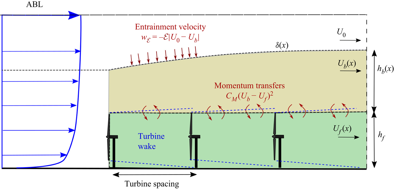
The present finite-length entrainment model is an extension of the three-layer approach introduced by Luzzatto-Fegiz & Caulfield (Reference Luzzatto-Fegiz and Caulfield2018) for ‘infinite’ wind farms. It is derived by assuming that all flow variables depend on the streamwise distance from the wind farm entrance (see figure 1). As a starting point, we use the Reynolds-averaged Navier–Stokes equations for a high-Reynolds-number boundary layer and assume flow homogeneity in the spanwise  $y$-direction. Additionally, we retain only leading terms in the momentum equation and obtain the following equations:
 $$\begin{gather} \frac{\partial \bar{u}}{\partial x} + \frac{\partial \bar{w}}{\partial z} =0, \end{gather}$$
 $$\begin{gather}\bar{u} \frac{\partial \bar{u}}{\partial x} + \bar{w} \frac{\partial \bar{u}}{\partial z} ={-}\frac{\partial \overline{u^\prime w^\prime}}{\partial z} + \bar{f}_x, \end{gather}$$
where bars, e.g.  $\bar {u}$, indicate the time-averaged fields and primes, e.g. $u^\prime =u-\bar {u}$, the turbulent fluctuations (dispersive terms are not shown in the derivation for brevity, but are included in the model through the parametrisation of the stresses; see Luzzatto-Fegiz & Caulfield Reference Luzzatto-Fegiz and Caulfield2018). The force term $f_x$ corresponds to the thrust of the wind turbines. Similar to Luzzatto-Fegiz & Caulfield (Reference Luzzatto-Fegiz and Caulfield2018), we assume that the following boundary conditions apply:
 \begin{equation} \left.\begin{gathered} \bar{w}(x,0)=0,\quad \bar{u}(x,\delta(x))=U_0,\quad \bar{w}(x,\delta(x))=U_0\dfrac{\mathrm{d} \delta(x)}{\mathrm{d}\kern0.7pt x}-\mathcal{E}|U_0-U_b(x)|, \\ -\overline{u^\prime w^\prime}(x,0)=\tau_{w}(x)/\rho,\quad -\overline{u^\prime w^\prime}(x,\delta(x))=0, \end{gathered}\right\} \end{equation}
where  $U_0$ is the velocity outside the boundary layer (representing the geostrophic wind), $\delta (x)$ is the boundary layer height, $\tau _w(x)$ is the shear stress at the ground and $\mathcal {E}$ is the entrainment coefficient. A three-layer model of the developing boundary layer is obtained by dividing it into an outer layer with velocity $U_0$, a wind farm layer of height $h_f$ and velocity $U_f(x)$, and a by-pass layer with height $h_b(x)$ and velocity $U_b(x)$, as shown in figure 1. Note here that the characteristic velocities of the wind farm and by-pass layers are functions of the streamwise position and are defined to be the integral velocities within each layer,
 \begin{equation} U_f (x) = \frac{1}{h_f}\int _0^{h_f} \bar{u}(x)\,\mathrm{d}z,\quad U_b (x) = \frac{1}{h_b(x)} \int _{h_f}^{\delta(x)} \bar{u}(x)\,\mathrm{d}z, \end{equation}
where  $h_f$ is the constant height from the ground to the wind farm layer interface and $h_b(x)$ is the height of the by-pass flow extending from the wind farm layer interface all the way up to the outer boundary layer (see figure 1). Note that throughout the wind farm, $h_f+h_b(x)=\delta (x)$. In line with the entrainment model of Luzzatto-Fegiz & Caulfield (Reference Luzzatto-Fegiz and Caulfield2018), $h_b$ is defined by
 \begin{equation} h_b(x) U_b^2(x) = \int_{h_f}^{\delta(x)} \bar{u}^2\,\mathrm{d}z. \end{equation}
This, together with the definition provided in (2.3a,b), defines the by-pass layer's thickness,  $h_b$, and its bulk velocity, $U_b$, in a fashion similar to how the momentum thickness of a boundary layer is defined in classic boundary layer theory (Schlichting Reference Schlichting1979). Moreover, we assume that the following approximate relationship holds in the wind farm layer:
 \begin{equation} \int _0^{h_f} \bar{u}^2\,\mathrm{d}z \approx h_f U_f^2(x). \end{equation}
The detailed derivation of the above equation is given in Appendix A. Note that  $h_b$ is defined so that it extends up to the edge of the atmospheric boundary layer, in a different spirit from conventional log-law models, where the upper layer extends to the internal boundary layer (e.g. Meneveau Reference Meneveau2012). In that way, we can make the assumption that $U_0$ is constant in space and that the outer layer is stress-free. In contrast, the internal boundary layer grows within the atmospheric boundary layer, which means that it develops within a varying mean velocity field, but also within varying turbulence levels. The former could be accounted for by computing $U_0(x)$ through the log law, by considering an additional layer in the model or by disregarding the evolution of the outer layer (i.e. $U_0(x)= U_0$). The latter, however, gives rise to the need for a more elaborate parametrisation of the entrainment coefficient $\mathcal {E}$ (which extends beyond the scope of the present study), as the assumption of it being constant with space becomes invalid, given that its values are known to vary with different ‘free stream’ turbulence levels (see Kankanwadi & Buxton Reference Kankanwadi and Buxton2020). Second, the assumption of $\mathcal {E}$ being independent of the farm layout is also not always true, given that the structure of the internal boundary layer in the development zone is a function of the farm layout. Nevertheless, it is important to note that considering the outer layer to be the internal boundary layer is a limit case for our model, with $h_b(0) \rightarrow 0$.
Schematic representation (not to scale) of the atmospheric boundary layer (ABL) and the turbulent entrainment model for finite-length wind farms.
We begin by integrating the continuity equation along the vertical  $z$-direction from the ground to the outer interface $\delta (x)$ and using Leibniz's rule to obtain
 \begin{align} \int _0^{\delta(x)} \frac{\partial \bar{u}}{\partial x} + \frac{\partial \bar{w}}{\partial z} \mathrm{d} z &= \frac{\mathrm{d}}{\mathrm{d}\kern0.7pt x} \int _0^{\delta(x)} \bar{u}\,\mathrm{d} z - \bar{u}_{z=\delta(x)} \frac{\mathrm{d} \delta(x)}{\mathrm{d}\kern0.7pt x} + \bar{w}_{z=\delta(x)} -\bar{w}_{z=0} \nonumber\\ &= \frac{\mathrm{d}}{\mathrm{d}\kern0.7pt x} \int _0^{\delta(x)} \bar{u}\,\mathrm{d} z - U_0 \frac{\mathrm{d} \delta(x)}{\mathrm{d}\kern0.7pt x} + U_0 \frac{\mathrm{d} \delta(x)}{\mathrm{d}\kern0.7pt x} + \overline{w_{\mathcal{E}}} = 0 \nonumber\\ &\Rightarrow\frac{\mathrm{d}}{\mathrm{d}\kern0.7pt x} \int _0^{\delta(x)} \bar{u}(x) \mathrm{d}z ={-}\overline{w_{\mathcal{E}}}, \end{align}
where  $\overline {w_{\mathcal {E}}}$ is the vertical velocity at $\delta (x)$ in the frame of reference moving with the outer boundary layer. Equation (2.6) signifies the essence of the model, which is that the boundary layer grows due to entrainment at the outer interface. The left-hand side of (2.6) can be reformulated using the above definitions as
 \begin{align} \frac{\mathrm{d}}{\mathrm{d}\kern0.7pt x} \int _0^{\delta(x)} \bar{u}\,\mathrm{d}z &= \frac{\mathrm{d}}{\mathrm{d}\kern0.7pt x} \int _0^{h_f} \bar{u}\,\mathrm{d}z + \frac{\mathrm{d}}{\mathrm{d}\kern0.7pt x} \int _{h_f}^{\delta(x)} \bar{u}\,\mathrm{d}z \nonumber\\ &= \frac{\mathrm{d}}{\mathrm{d}\kern0.7pt x} [U_f(x) h_f + U_b(x) h_b(x)]. \end{align}
For the right-hand side of (2.6), we make use of the entrainment hypothesis, which states that  $\overline {w_{\mathcal {E}}} = - \mathcal {E} |U_0-U_{b}(x)|$, where $\mathcal {E}$ is the entrainment coefficient and $U_0$ and $U_{b}(x)$ are characteristic velocities across the boundary layer interface (with $U_0>U_b(x)$). The final expression for continuity can now be obtained:
 \begin{equation} \frac{\mathrm{d}}{\mathrm{d}\kern0.7pt x} (h_b U_b) = \mathcal{E} (U_0-U_b) - h_f \frac{\mathrm{d} U_f}{\mathrm{d}\kern0.7pt x}. \end{equation}
For the momentum equation, we adopt a similar approach but integrate the two layers separately. Starting with the left-hand side for the wind farm zone and using the approximation (2.5), we obtain
 \begin{equation} \int _0^{h_f} \left(\frac{\partial \bar{u}^2}{\partial x} + \frac{\partial \bar{u} \bar{w}}{\partial z} \right)\mathrm{d}z = h_f \frac{\mathrm{d}U_f^2}{\mathrm{d}\kern0.7pt x} + \left(\bar{u} \bar{w} \right)_{z=h_f}-\left(\bar{u} \bar{w} \right)_{z=0}. \end{equation}
To compute the second term, the streamwise velocity at the farm interface (denoted by  $\bar {u}_{h_f} = \bar {u} _{z={h_f}}$) is approximated by assuming a mixing layer velocity, $\bar {u}_{h_f} = (U_f + U_b)/2$ (see also Luzzatto-Fegiz & Caulfield Reference Luzzatto-Fegiz and Caulfield2018). For the vertical velocity at the same interface, we also make use of the integrated continuity equation for the wind farm zone, which writes
 \begin{equation} \bar{w}_{h_f} ={-} h_f \frac{\mathrm{d}U_f}{\mathrm{d}\kern0.7pt x}. \end{equation}
The terms on the right-hand side of the momentum equation are integrated to obtain
 \begin{align} \int _0^{h_f} \left(-\frac{\partial \overline{u^\prime w^\prime}}{\partial z} + \bar{f}_x \right) \mathrm{d} z =\left( - \overline{u'w'} \right)_{z=h_f} - \frac{\tau_w}{\rho} + \int _0^{h_f} f_x\,\mathrm{d}z = C_M \left(U_b - U_f \right)^2 - \frac{c^\prime_{ft}+c^\prime_d}{2} U_f^2, \end{align}
where  $C_M$ is a momentum-exchange coefficient used in the parametrisation of the stresses at the farm layer interface as $(-\overline {u'w'})_{z=h_f} = C_M (U_b - U_f )^2$ (see also Luzzatto-Fegiz & Caulfield Reference Luzzatto-Fegiz and Caulfield2018), and $c^\prime _{ft}$ and $c^\prime _d$ are the local turbine thrust and ground drag coefficients. These are defined as by Luzzatto-Fegiz & Caulfield (Reference Luzzatto-Fegiz and Caulfield2018):
 \begin{equation} c^\prime_{ft} ={-} \frac{2}{U_f^2} \int _0^{h_f} f_x\,\mathrm{d}z = \frac{C_T {\rm \pi}}{s_x s_y \left(1+ \sqrt{1-C_T} \right)^2} \end{equation}
and
 \begin{equation} c^\prime_d = \frac{2 \tau_w}{\rho U_f^2} = \frac{2 \kappa^2}{\left(1+\ln{\left(z_0/h_f\right)} \right)^2}, \end{equation}
where  $s_x$ and $s_y$ are the turbine array spacings (normalised by the turbine diameter $D$) along the streamwise and spanwise directions, respectively, $C_T$ is the turbine thrust coefficient, $z_0$ is the ground roughness length and $\kappa$ is the von Kármán constant. The expression for momentum conservation in the wind farm zone is therefore
 \begin{equation} h_f \frac{\mathrm{d} U_f^2}{\mathrm{d}\kern0.7pt x} - \frac{(U_f+U_b)}{2} h_f \frac{\mathrm{d} U_f}{\mathrm{d}\kern0.7pt x} = C_M \left( U_b - U_f \right)^2 - \frac{c^\prime_{ft}+c^\prime_d}{2} U_f^2. \end{equation}
In a similar manner, integrating the left-hand side of the momentum equation within the by-pass zone yields
 \begin{align} \int _{h_f}^{\delta(x)} \left( \frac{\partial \bar{u}^2}{\partial x} + \frac{\partial \bar{u} \bar{w}}{\partial z} \right)\mathrm{d}z &= \frac{\mathrm{d}}{\mathrm{d}\kern0.7pt x} \int _{h_f}^{\delta(x)} \bar{u}^2\,\mathrm{d}z - \bar{u}^2_{z=\delta(x)} \frac{\mathrm{d} \delta(x)}{\mathrm{d}\kern0.7pt x} + \left( \bar{u} \bar{w} \right)_{z=\delta(x)} - \left( \bar{u} \bar{w} \right)_{z=h_f} \nonumber\\ &= \frac{\mathrm{d} (h_b U_b^2)}{\mathrm{d}\kern0.7pt x} -\mathcal{E} (U_0-U_b) U_0 + \frac{U_f+U_b}{2} h_f \frac{\mathrm{d} U_f}{\mathrm{d}\kern0.7pt x}. \end{align}
Integrating the right-hand side yields
 \begin{equation} \int _{h_f}^{\delta(x)} \left(-\frac{\partial \overline{u^\prime w^\prime}}{\partial z} + \bar{f}_x \right) \mathrm{d} z ={-}(\overline{u^\prime w^\prime})_{z=\delta(x)} + (\overline{u^\prime w^\prime})_{z=h_f} ={-}C_M(U_b-U_f)^2, \end{equation}
where we use both the layer boundary conditions and the fact that the turbine forcing is zero outside of the wind farm layer. The final expression for the momentum equation in the by-pass zone is obtained by moving all terms, other than the streamwise rate of change of  $h_b U_b^2$, to the right-hand side:
 \begin{equation} \frac{\mathrm{d} \left( h_b U_b^2 \right)}{\mathrm{d}\kern0.7pt x} = \mathcal{E} U_0 (U_0-U_b) - C_M (U_b - U_f)^2 - \frac{(U_f+U_b)}{2} h_f \frac{\mathrm{d} U_f}{\mathrm{d}\kern0.7pt x}. \end{equation}
Equations (2.8), (2.14) and (2.17) form a system of ordinary differential equations with three unknowns ( $h_b$, $U_b$ and $U_f$), which is an initial value problem that can be solved numerically given that the entrainment coefficient, $\mathcal {E}$, and momentum transfer coefficient, $C_M$, are known along with the turbine thrust, row spacing and ground wall drag coefficient. In the present work, the system is solved using MATLAB's ode45 solver, which is based on a high-order Runge–Kutta algorithm (Shampine & Reichelt Reference Shampine and Reichelt1997). The values of $U_f$ and $U_b$ upstream of the farm that act as initial conditions for the model are computed by considering a fully developed unperturbed atmospheric boundary layer, i.e. the three-layer model at the fully developed limit without wind turbines ( $c^\prime _{ft}=0$). The initial by-pass height, $h_b(0)=\delta (0)-h_f$, is calculated via the initial boundary layer height, $\delta (0)$, and the constant wind farm height, $h_f$. Note that at the fully developed limit, the wind farm velocity, $U_f$, is no longer evolving and therefore the system of equations reduces to that of Luzzatto-Fegiz & Caulfield (Reference Luzzatto-Fegiz and Caulfield2018).
Using actuator disc theory, the extracted power may be expressed as  $P=T U_f$ (with $T=0.5 \rho c^\prime _{ft} U_f^2 s_x s_y D^2$ denoting the turbine thrust), and thus the entrainment model can be used to predict the power production along the farm:
 \begin{equation} c_{fp} = \frac{P}{\dfrac{1}{2} \rho U_0^3 s_x s_y D^2} = c^\prime_{ft} \left( \frac{U_f}{U_0} \right)^3, \end{equation}
where  $c_{fp}$ is the non-dimensional power density coefficient.
Additionally, the model can give predictions for the mechanisms of energy transport (i.e. advection or turbulent transport) in the wind farm zone. The mean-flow kinetic energy equation can be derived by multiplying the momentum equation by the mean velocity (Pope Reference Pope2000); see also § 4.4 for the full equation and a description of the terms of which it consists. Integrating the advection and turbulent transport terms (denoted by  $A$ and $\varPhi$, respectively) within an infinitesimal control volume $V$ of size $\mathrm {d}\kern0.7pt x \times \mathrm {d}y \times h_f$ in the wind farm zone yields
 \begin{equation} A ={-} \int_V \overline{u_j} \frac{\partial \bar{K}}{\partial x_j}\, \mathrm{d} V,\quad \varPhi ={-} \int_V \frac{\partial \left(\overline{u_i} \overline{u_i^\prime u_j^\prime} \right)}{\partial x_j}\, \mathrm{d} V, \end{equation}
where  $\bar {K}= \overline {u_i}\, \overline {u_i}/2$ is the mean-flow kinetic energy. Using the divergence theorem, these can be transformed to surface integrals
 \begin{equation} A ={-} \int_S \overline{u_i} \bar{K} n_i \,\mathrm{d} S,\quad \varPhi ={-} \int_S \overline{u_i} \overline{u_i^\prime u_j^\prime} n_j\,\mathrm{d} S, \end{equation}
where  $n_i$ is the unit vector normal to the surface $S$ of the control volume. In the framework of the model, which involves the assumptions of spanwise homogeneity and retains only the leading stress terms, the above are expressed as
 $$\begin{gather} \frac{A}{\mathrm{d}\kern0.7pt x\, \mathrm{d}y} ={-}\frac{\mathrm{d}}{\mathrm{d}\kern0.7pt x} \int _0^{h_f} \bar{u} \bar{K}\,\mathrm{d} z - \left(\bar{w} \bar{K} \right)_{z=h_f} + \left(\bar{w} \bar{K} \right)_{z=0} \approx{-} \frac {1}{2} h_f \frac{\mathrm{d} U_f^3}{\mathrm{d}\kern0.7pt x} - \left( \bar{w} \bar{K} \right)_{z=h_f}, \end{gather}$$
 $$\begin{gather}\frac{\varPhi}{\mathrm{d}\kern0.7pt x\,\mathrm{d}y} = C_M \left(U_b-U_f \right)^2 \bar{u}_{h_f} - \left(c^\prime_d/2 \right) U_f^3. \end{gather}$$
The first component of the advection term,  $A$, corresponds to the upstream/downstream surfaces of the control volume and includes an approximation of the integral using the assumptions $\bar {u}^2 \gg \bar {w}^2$ and $\int _0^{h_f} (\bar {u}-U_f )^3 \,\mathrm {d} z \ll \int _0^{h_f} U_f^3 \,\mathrm {d} z$, in a process similar to the derivation presented in Appendix A. The second and third terms correspond to the upper and lower control volume surfaces, respectively. The transport of the mean kinetic energy by turbulence, $\varPhi$, takes place at both the farm layer interface and the aerodynamically rough ground. In the remainder of this work, however, we will be considering the transfers at the top surface of the wind farm layer only, as our focus is on the interaction of the wind farm with the atmospheric flow.
2.2. Model demonstration
To assess the applicability of our model and its compatibility with Luzzatto-Fegiz & Caulfield (Reference Luzzatto-Fegiz and Caulfield2018) in the ‘infinite’ wind farm limit, we present an example of a finite-length wind farm by considering the values used by Luzzatto-Fegiz & Caulfield (Reference Luzzatto-Fegiz and Caulfield2018). These are  $\mathcal {E}=0.16$, $C_M=0.04$, $c^\prime _d=0.008$ (which corresponds to $h_f/D=1.5$ and $z_0/D=10^{-3}$) and $C_T=0.75$. We also take $\delta (0)/z_h=10$ and $s_x=s_y=6$. A sensitivity study on the empirical parameters $\mathcal {E}$ and $C_M$ is presented separately in Appendix B. Differences in the exact values of the coefficients are shown to affect the magnitude of power output predicted by the model, as observed by Luzzatto-Fegiz & Caulfield (Reference Luzzatto-Fegiz and Caulfield2018), but flow development occurs in a similar manner. Figure 2 shows the predictions of the model for a wind farm consisting of 50 rows and compares them with the ‘infinite-farm’ predictions given by Luzzatto-Fegiz & Caulfield (Reference Luzzatto-Fegiz and Caulfield2018). The characteristic velocities of both wind farm and by-pass zones decrease monotonically as we move downstream in the farm and asymptotically approach the ‘infinite-farm’ predictions of Luzzatto-Fegiz & Caulfield (Reference Luzzatto-Fegiz and Caulfield2018). In addition, the wind farm velocity, $U_f$, decreases rapidly within the first 10 rows, which is subsequently reflected in the normalised power density, $c_{fp}$. The model predicts that for the given coefficients and turbine parameters, the wind farm power output in the ‘infinite-length’ limit is approximately 0.4 times that of the first row, which is within the range observed in utility-scale offshore wind farms (see, for example, Barthelmie et al. Reference Barthelmie2007). In terms of energy transport (with the terms integrated over $s_xD$ and $s_yD$), our model predicts that advection is the dominant mechanism in the first few rows of turbines, but it is subsequently reduced and becomes practically zero by approximately the tenth row. At the same time, turbulent transport grows in the initial rows, with a peak observed around the tenth row, before decreasing as we proceed further downstream. These trends are in agreement with the observations in the computational studies of Allaerts & Meyers (Reference Allaerts and Meyers2017) and Cortina et al. (Reference Cortina, Sharma, Torres and Calaf2020).
Predictions of the finite-length entrainment model for a wind farm of 50 rows. The dashed lines correspond to the ‘infinite-farm’ predictions of Luzzatto-Fegiz & Caulfield (Reference Luzzatto-Fegiz and Caulfield2018).
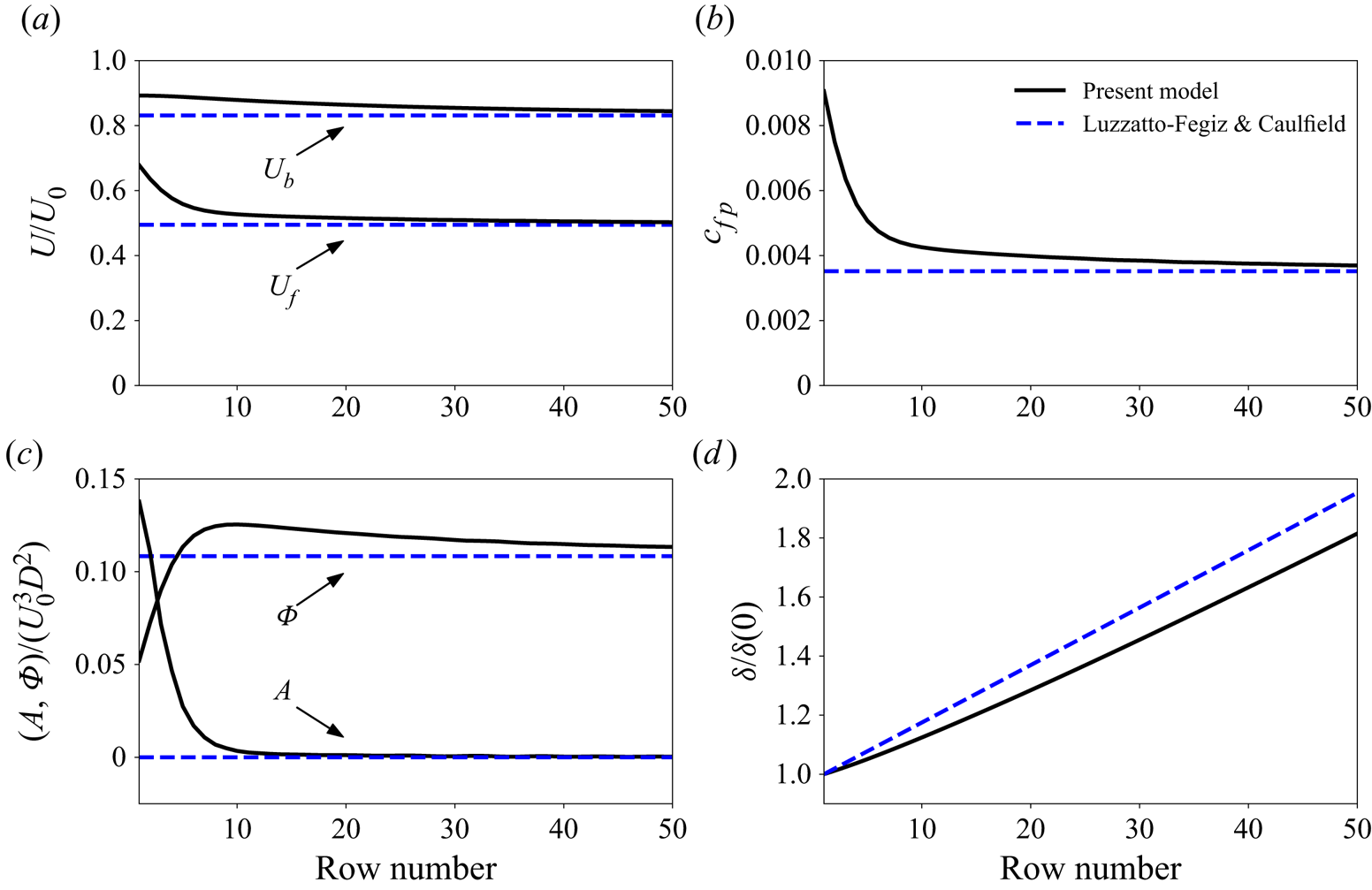
Lastly, the boundary layer is predicted to grow at a slightly lower rate in the developing part of the flow, which can be associated with the fact that the bulk velocities are also developing. Nevertheless, all the quantities of interest ( $U_f$, $U_b$, $c_{fp}$, $A$,
$A$,  $\varPhi$ and $\mathrm {d} \delta / \mathrm {d}\kern0.7pt x$) are found to asymptotically approach their ‘infinite-farm’ limit values as calculated in the work of Luzzatto-Fegiz & Caulfield (Reference Luzzatto-Fegiz and Caulfield2018), confirming that the present finite-length model is fully compatible with the original ‘infinite-farm’ entrainment model.
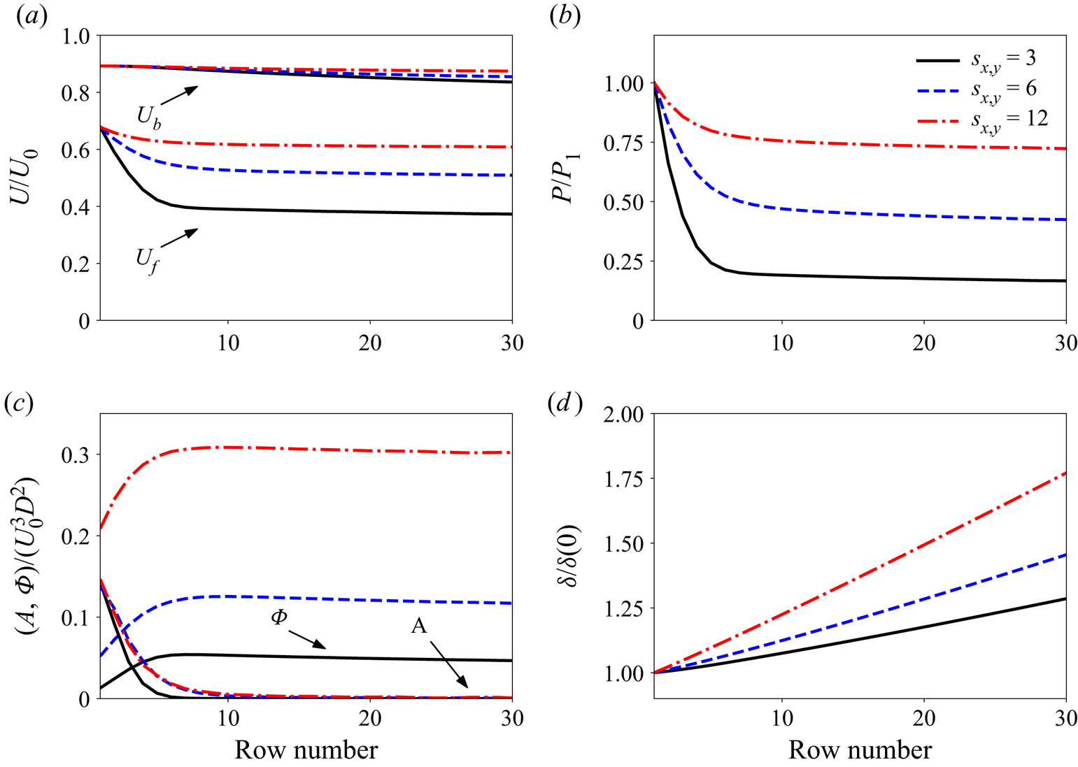
Next, we proceed to vary key parameters of the finite-length wind farm model such as the wind turbine array spacing ( $s_{x,y}=3,6$ and 12), as shown in figure 3. As expected, a larger turbine spacing allows for increased replenishment of energy between successive rows and downstream turbines are able to produce more power. However, the opposite effect is achieved once the turbine rows come closer, reaching a power reduction of 80 % after approximately the seventh row. Variations in the height of the incoming boundary layer
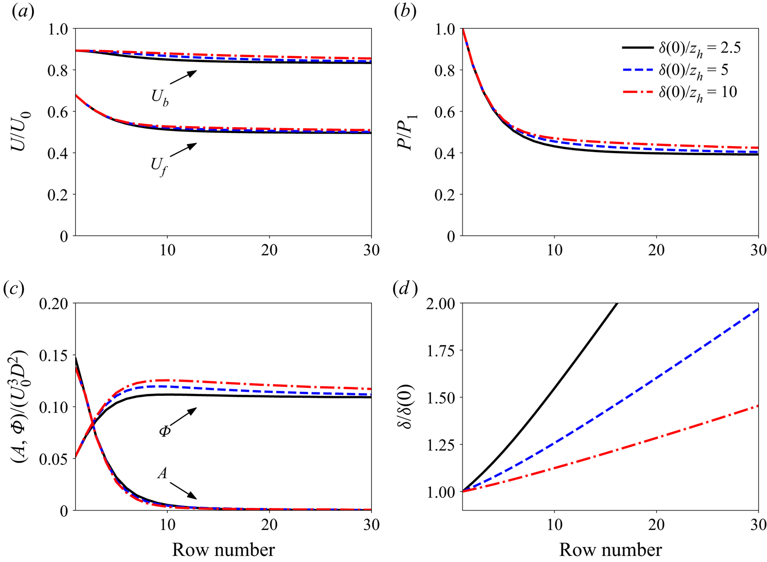
  $\delta (0)$ are considered next, namely, $\delta (0)/z_h=2.5$, 5 and 10. Allaerts & Meyers (Reference Allaerts and Meyers2017) found variations in the power output with boundary layer height, with larger heights resulting in slightly increased farm power. The differences were attributed to the amounts of energy transport by turbulence. Our simplified model (see figure 4) is able to reproduce this behaviour prior to reaching the ‘infinite-farm’ limits (which are the same in all three cases). We find that small changes are observed in mean velocity and relative wind farm power output, $P/P_1$, and that the turbulent energy flux, $\varPhi$, is negatively affected by a diminishing boundary layer height to hub height ratio. More specifically, the wind farm velocity is only little affected by the initial boundary layer height, whereas the by-pass velocity is shown to decay and adjust to its limit value faster with a decreasing initial boundary layer height. Figure 4 also shows that a smaller initial boundary layer height results in faster growth of its magnitude downstream of the entrance. Finally, an initially larger boundary layer height $\delta$ results in larger turbulent transport as indicated by the magnitude of $\varPhi$. This behaviour may again be justified by the relative changes in the magnitudes of $U_f$ and $U_b$ and the fact that $\varPhi \propto (U_b-U_f)^2$.
Model predictions for wind farms with different turbine spacings  $s_{x,y}=3,6$ and 12.
Model predictions for different inflow boundary layer heights  $\delta (0)/z_h=2.5, 5$ and 10.
2.3. Comparison with field and model wind farm data
Prior to comparing our model results with large-eddy simulation data, we make comparisons with experimental data and existing analytical models found in the literature. In particular, comparisons are made against a model of equal fidelity, i.e. the top-down model with entrance effects (Meneveau Reference Meneveau2012), and wind farm power measurements at both utility and laboratory scale. The analytical model of Meneveau (Reference Meneveau2012) represents the wind farm effect through an effective roughness model, reflected in the modified friction velocity,  $u_*$. In addition, wind farm entrance effects are incorporated by assuming a transition from a smoother to a rougher turbulent boundary layer and the formation of an internal boundary layer (IBL) that follows a $4/5$ growth rate with the downstream distance. The wind farm field and laboratory measurements include the Horns Rev I offshore wind farm, located in the North Sea (Barthelmie et al. Reference Barthelmie2007), and a wind-tunnel-scale wind farm set up and studied in the Corrsin Wind Tunnel at Johns Hopkins University (Bossuyt, Meneveau & Meyers Reference Bossuyt, Meneveau and Meyers2018a). Horns Rev I consists of eighty turbines with $D=80$ m, $z_h=70$ m and $C_T=0.7$, arranged in a $8\times 10$ grid (Meneveau Reference Meneveau2012). Data for the boundary layer are taken from Wu & Porté-Agel (Reference Wu and Porté-Agel2015), with $u_*=0.442$ m s $^{-1}$, $z_0=0.05$ m and $\delta (0)=500$ m. The model wind farm of Bossuyt et al. (Reference Bossuyt, Meneveau and Meyers2018a) consists of 100 turbines arranged in a $20 \times 5$ array. For more details about the turbines and boundary layer, the reader is referred to Bossuyt et al. (Reference Bossuyt, Meneveau and Meyers2018a).
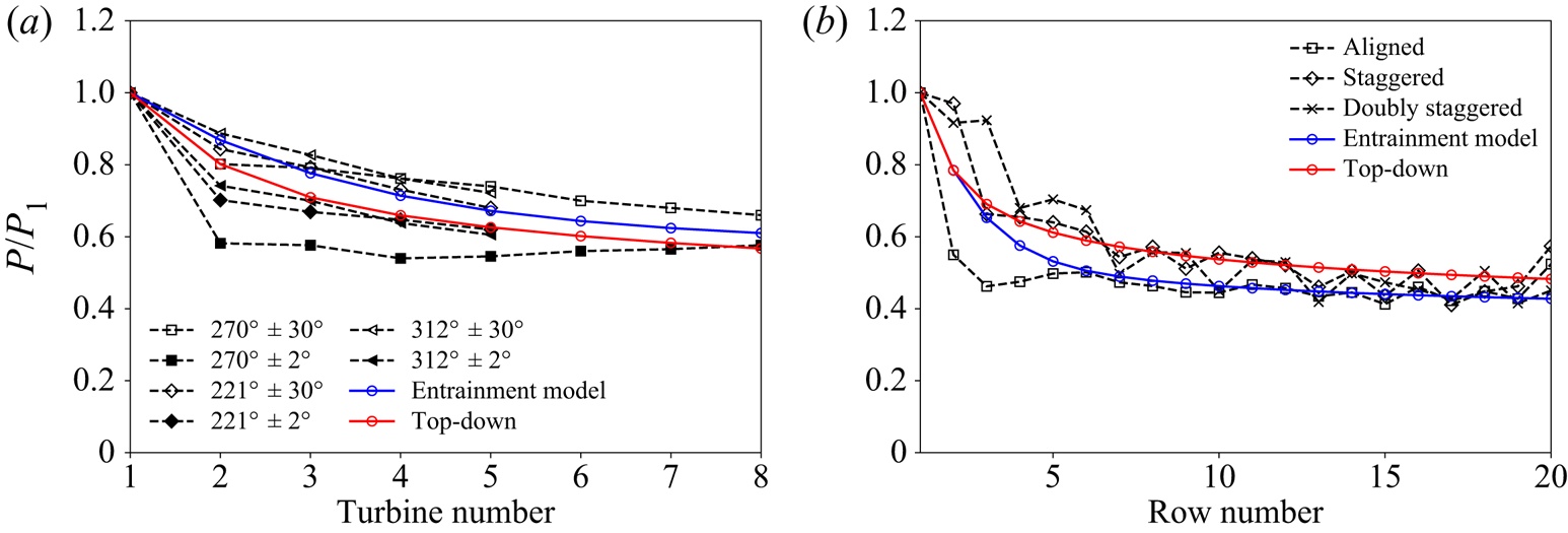
Figure 5 shows the power deficit along the turbine rows for different wind directions and measurement sectors in the case of the Horns Rev I wind farm (that effectively correspond to different arrangements) and for different farm layouts in the case of the model wind farm. In both cases, the values  $\mathcal {E}=0.16$ and $C_M=0.04$ are used in the finite-length entrainment model (see Luzzatto-Fegiz & Caulfield Reference Luzzatto-Fegiz and Caulfield2018). The two models show comparable accuracy, and both display good agreement with the field and wind tunnel measurements. For the Horns Rev wind farm case, the power predictions of the present model are slightly higher than the power obtained for the top-down model with entrance effects (Meneveau Reference Meneveau2012) while an opposite trend is reported for the model wind farm of Bossuyt et al. (Reference Bossuyt, Meneveau and Meyers2018a). We note here that one may reduce the difference between the two models by tuning the parameters of each model. Another interesting observation is that, in both cases, a marginally better agreement is found for the cases of (effectively) staggered configurations; this is related to the two models’ ‘well-mixed’ flow assumption.
Normalised power output for (a) the Horns Rev I wind farm (measurements as reported in Barthelmie et al. Reference Barthelmie2007) and (b) the model wind farm of Bossuyt et al. (Reference Bossuyt, Meneveau and Meyers2018a). Also shown are the predictions of the finite-length entrainment model and the top-down model with entrance effects (Meneveau Reference Meneveau2012).
On a higher level, we note that our model can predict wind farm power degradation without assuming either a growth rate for the IBL or requiring the far-upstream velocity field to follow the logarithmic law within the boundary layer. This allows us to further generalise our model and better interpret its results. Inherently, the imposition of an upstream boundary layer height,  $\delta (0)$, and wall roughness, $z_0$, under neutral conditions will give rise to a logarithmic profile, but these are only implicit in our model. However, our model does depend on two ad hoc parameters, namely the turbulent entrainment, $\mathcal {E}$, and the momentum exchange coefficient, $C_M$. These can be easily interpreted as bulk flow quantities that enable mixing between the assumed sublayers. Following the discussion of Luzzatto-Fegiz & Caulfield (Reference Luzzatto-Fegiz and Caulfield2018), both $\mathcal {E}$ and $C_M$ can be linked to the Obukhov length scale and therefore the boundary layer stability. In particular, $\mathcal {E}$ can vary from ${O}(1\times 10^{-4})$ for very stable boundary layers to $\mathcal {E}\approx 0.16$ for conventionally neutral conditions. In the same study, the momentum exchange coefficient, $C_M$, is shown to be weakly related to $\mathcal {E}$. An interesting observation can be made for the boundary layer growth by looking at the growth rate of the external layer, $\delta /\delta (0)$, presented in Appendix B. A 20 % difference in the value of $\mathcal {E}$ is found to affect the growth rate of $\delta$, a result which can be inherently linked back to its very definition.
3. The large-eddy simulation flow solver
3.1. Governing equations
To assist our analysis and understanding of the entrainment model parameters, we gather high-fidelity data by conducting a series of large-eddy simulations. In particular, we use WInc3D (Deskos, Laizet & Palacios Reference Deskos, Laizet and Palacios2020), a wind farm simulator, which is part of the high-order direct and large-eddy simulation (LES) framework XCompact3D (Bartholomew et al. Reference Bartholomew, Deskos, Frantz, Schuch, Lamballais and Laizet2020). The equations governing the wind farm flow dynamics are the unsteady, incompressible, filtered Navier–Stokes equations expressed in the skew-symmetric form
 $$\begin{gather} \frac{\partial \tilde{u}_i}{\partial x_i}=0, \end{gather}$$
 $$\begin{gather}\frac{\partial \tilde{u}_i}{\partial t}+\frac{1}{2}\left(\tilde{u}_j\frac{\partial \tilde{u}_i}{\partial x_j} + \frac{\partial \tilde{u}_i \tilde{u}_j}{\partial x_j}\right)={-}\frac{1}{\rho}\frac{\partial \tilde{p}}{\partial x_i}-\frac{\partial \tau_{ij}}{\partial x_j} + \frac{f_i^T}{\rho}. \end{gather}$$
The tilded variables  $\tilde {p}$ and $\tilde {u}_i=(u_x,u_y,u_z)$ are the spatially filtered components of modified pressure and velocity, respectively, and $\rho$ is the fluid density, which is considered to be constant. We note that the viscous terms have been omitted, as is typical in relevant studies, due to the high-Reynolds-number nature of the considered flows. The term $-\partial _j \tau _{ij}$ present in the momentum equation is the subfilter-scale flux, which is computed via the standard Smagorinsky model (Smagorinsky Reference Smagorinsky1963)
 \begin{equation} \tau_{ij}={-}2 \nu_T \tilde{S}_{ij},\quad \nu_T= (C_S \varDelta)^2 |\tilde{S}|, \end{equation}
where
 \begin{equation} \tilde{S}_{ij}=\frac{1}{2}\left(\frac{\partial \tilde{u}_i}{\partial x_j} + \frac{\partial \tilde{u}_j}{\partial x_i} \right) \end{equation}
is the strain-rate tensor,  $|\tilde {S}|$ is its magnitude and $\varDelta$ is the grid size. A shear-stress model is applied on the bottom wall,
 \begin{equation} \tau^{wall}(x,y,t)=\tau_w(x,y,t)\frac{\hat{\tilde{u}}_i(x,y, \Delta z/2, t)}{\sqrt{\hat{\tilde{u}}_x^2(x,y,\Delta z/2, t)+ \hat{\tilde{u}}_y^2(x,y,\Delta z/2 ,t)}}, \end{equation}
with
 \begin{equation} \tau_w(x,y,t)={-}\left[\frac{\kappa}{\ln \left(\dfrac{\Delta z /2}{z_0}\right)}\right]^2 [\hat{\tilde{u}}_x^2(x, y,\Delta z/2,t)+\hat{\tilde{u}}_y^2(x, y,\Delta z/2,t)], \end{equation}
where  $z_0$ and $\kappa =0.4$ are the wall roughness and the von Kármán constant, respectively. The $\widehat {\dots }$ denotes a Gaussian test filter corresponding to twice the grid size, $\tilde {\varDelta }=2\varDelta$, following the formulation of Bou-Zeid, Meneveau & Parlange (Reference Bou-Zeid, Meneveau and Parlange2005). Finally, the Smagorinsky coefficient $C_S$ is adjusted near the wall according to the damping function of Mason & Thomson (Reference Mason and Thomson1992),
 \begin{equation} C_S=\left(C_0^{{-}n}+\left\{\kappa \left( \frac{z}{\varDelta}+ \frac{z_0}{\varDelta}\right) \right\}^{{-}n}\right)^{{-}1/n}, \end{equation}
with  $(C_0, n)=(0.14,3)$. The above equations are discretised using sixth-order compact finite-difference schemes on a Cartesian mesh in a half-staggered arrangement and a second-order Adams–Bashforth method for time advancement (Laizet & Lamballais Reference Laizet and Lamballais2009). Parallelisation is achieved with the highly scalable 2Decomp & FFT library that implements a two-dimensional pencil decomposition of the computational domain (Laizet & Li Reference Laizet and Li2011).
3.2. Wind turbines parametrisation
Wind turbines are parametrised using an actuator disk model (ADM), which accounts for the total thrust force experienced by the turbine blades,
 \begin{equation} F_T={-}\frac{1}{2}\rho C_T U_\infty^2 \frac{\rm \pi}{4} D^2, \end{equation}
where  $C_T$ is the thrust coefficient, $U_\infty$ the upstream turbine velocity and $D$ the rotor diameter. The ADM is implemented using a methodology identical to that presented by Calaf et al. (Reference Calaf, Meneveau and Meyers2010). More specifically, the force per unit mass which is added to the right-hand side of the filtered momentum equation (3.2),
 \begin{equation} \frac{f_i^T}{\rho}={-}\frac{1}{2} C_T' V^2 \frac{\gamma(x,y,z)}{\Delta x}, \end{equation}
is calculated by assuming an induction factor  $\alpha$ and a thrust coefficient $C_T$ and using
 \begin{equation} C'_T=\frac{C_T}{(1-\alpha)^2}. \end{equation}
Here, the coefficient  $\gamma (x,y,z)$ represents the rotor region and takes values between 0 and 1. Actuator discs are allowed to have a width equal to the size of one cell, while their mesh frontal area is computed as the fraction of the area that overlaps between the cell grid points and the rotor ( $\gamma =1$ if the mesh point lies within the rotor, $\gamma =0$ if it lies outside and $\gamma$ takes an intermediate value for adjacent mesh nodes). The rotor velocity $V$ is evaluated by spatially averaging over all grid points in the wind turbine disc and time-averaging (filtering) to ensure that high-frequency velocity oscillations do not affect the rotor's thrust. The process for computing the space/time-averaged velocity $V$ is the following:
 \begin{equation} V^{n}=\alpha_{rel} \langle \tilde{u}\rangle_d +(1-\alpha_{rel}) V^{n-1},\quad \alpha_{rel}=\frac{\Delta t}{\mathcal{T}}/\left(1+\frac{\Delta t}{\mathcal{T}}\right), \end{equation}
where  $n$ and $n-1$ denote the current and previous time steps, respectively, $\langle \tilde {u}\rangle _d$ denotes the disc-averaged velocity, $\alpha _{rel}$ is the relaxation coefficient and $\Delta t$ and $\mathcal {T}$ are the time step and time window used for averaging, respectively. In previous studies (Calaf et al. Reference Calaf, Meneveau and Meyers2010; Stevens, Gayme & Meneveau Reference Stevens, Gayme and Meneveau2014a; VerHulst & Meneveau Reference VerHulst and Meneveau2014), the time scale $\mathcal {T}$ used for the low-pass filtering is associated to either the turbine or the boundary layer length and velocity scales. Here, we adopt a time scale as in Calaf et al. (Reference Calaf, Meneveau and Meyers2010), $\mathcal {T}=0.27 \delta _0/u_*$, where $\delta _0$ is the height of the incoming boundary layer and $u_*$ the friction velocity. Finally, the power output of a turbine is computed using the local thrust,
 \begin{equation} P=\frac{1}{2} \rho C'_T V^3 \frac{\rm \pi}{4} D^2. \end{equation}
3.3. The ‘inflow-recirculation’ technique
To simulate the interaction of the wind farm with atmospheric turbulence, a fully developed turbulent field is needed to represent the inlet conditions. Here, we employ a ‘single-simulation’ strategy, in which the ‘precursor’ neutral atmospheric boundary layer and wind farm regions are parts of a single computational domain, thus allowing periodic boundary conditions to be used in the horizontal directions  $x$ and $y$. Our approach is similar to but slightly different from the one used by Bossuyt, Meneveau & Meyers (Reference Bossuyt, Meneveau and Meyers2018b) or Stevens, Graham & Meneveau (Reference Stevens, Graham and Meneveau2014b), where two separate but concurrent simulations (the precursor and the wind farm one) are performed. The ‘precursor’ atmospheric flow is driven by a constant pressure gradient, added to the right-hand side of (3.2). In addition, a ‘damping layer’ is used to restrict the development of the boundary layer beyond the desired inlet height $\delta _0$ and enforce a laminar region in the outer zone. The damping layer is applied in the precursor part of the computational domain through a forcing term added to the right-hand side of the momentum equation,
 \begin{equation} F_i^{{damp}}={-}\gamma \psi(z) \frac{u_*}{\delta_0} \left(\tilde{u}_i-G\right), \end{equation}
where  $G$ is the target velocity (here computed analytically via the log law), $\gamma$ a constant (taken to be 5 in this work) and $\psi (z)$ a vertical interpolation function,
 \begin{equation} \psi(z) =
\left\{\begin{array}{@{}ll} 0, & 0 \le z< 0.95
\delta_0, \\ \dfrac{1}{2}\left[1-\cos\left({\rm \pi}
\dfrac{z-0.95 \delta_0}{0.1 \delta_0} \right)\right], &
0.95 \delta_0 \le z < 1.05 \delta_0, \\ 1, & z\ge
1.05 \delta_0. \end{array}\right.
\end{equation}
\begin{equation} \psi(z) =
\left\{\begin{array}{@{}ll} 0, & 0 \le z< 0.95
\delta_0, \\ \dfrac{1}{2}\left[1-\cos\left({\rm \pi}
\dfrac{z-0.95 \delta_0}{0.1 \delta_0} \right)\right], &
0.95 \delta_0 \le z < 1.05 \delta_0, \\ 1, & z\ge
1.05 \delta_0. \end{array}\right.
\end{equation}To achieve a recirculation of the ‘precursor’ part of the domain (controlled ABL region), a ‘fringe region’ is used to allow the reinjection of the undisturbed upstream flow downstream of the wind farm. In particular, the fringe region is placed at the end of the computational domain to interpolate the velocity field between the unperturbed pre-farm atmospheric turbulence region and the post-farm wake region. The influence of the ABL in the post-farm region is gradually increased using the following weight function:
 \begin{equation} \lambda(x) = \left\{\begin{array}{@{}ll} 0, & 0 \le x< L_s, \\ \dfrac{1}{2}\left[1-\cos\left(\dfrac{4 {\rm \pi}}{3} \dfrac{x-L_s}{ \Delta L} \right)\right], & L_s \le x< L_e-\Delta L/4, \\ 1, & L_e-\Delta L/4 \le x < L_e, \end{array}\right. \end{equation}
where  $L_s$, $L_e$ and $\Delta L=L_e-L_s$ denote the start, end and length of the fringe region, respectively. Conversely, the post-farm velocity field is gradually decreased by multiplying it by the residual term, $1-\lambda (x)$. More specifically, the velocity field in the post-farm fringe region (indicated with the subscript $()_{{post}}$) is calculated as
 \begin{equation} \tilde{u}(x_{{post}}) =\lambda(x_{{ABL}}) \tilde{u}_{{ABL}}+ (1-\lambda(x_{{post}})) \tilde{u}_{{post}} \end{equation}
for  $L_s^{ABL} \le x_{{ABL}} \le L_e^{ABL}$ and $L_s^{post} \le x_{{post}} \le L_e^{post}$, with the superscripts representing the ABL and post-farm regions. Note that for the fringe-region approach to be applied, the lengths of the two regions should be exactly the same, i.e. $\Delta L^{ABL}=\Delta L^{post}$. Finally, to avoid the appearance of statistical inhomogeneities due to the spanwise locking of large-scale turbulent structures, we make use of the shifted periodic technique proposed by Munters, Meneveau & Meyers (Reference Munters, Meneveau and Meyers2016). Thus, three fringe regions may be identified in the domain: an ABL fringe region that is used as the ‘donor’ region, the pre-farm ‘receptor’ region where the shifted periodic technique is applied and, finally, the post-wind-farm region, which is another ‘receptor’ region where the flow is readjusted back to upstream turbulence before it is circulated to the beginning of the domain via the domain's periodic boundaries. The shifted periodic technique is implemented using the same weight function as with the ABL and post-wind-farm part presented in (3.16). Schematically, the implementation of the damping layer, ‘donor’ and shifted periodic and post-farm ‘receptor’ regions is presented in figure 6.
Schematic representation of the computational domain in the employed single-simulation strategy. The precursor, fringe and damping layer regions are coloured in light, medium and dark blue, respectively. The patterned area represents the region of the precursor that is used as ‘donor’ in the ‘recirculation’ and ‘shifted periodic’ techniques.
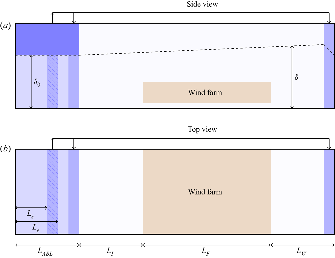
3.4. Validation study
The described methodology is validated against data from an experimental study considering boundary layers developing over finite-length model wind farms (Bossuyt et al. Reference Bossuyt, Howland, Meneveau and Meyers2017). To this end, we perform simulations of the flow over an aligned wind farm consisting of 20 rows in the streamwise direction and five turbines in the spanwise direction. The spacing between the turbines is  $s_x=7$ in the streamwise direction and $s_y=5$ in the spanwise one. The turbine diameter and hub height are $D=0.03$ m and $z_h = 0.023$ m, respectively, and $C'_T = 1.33$. The computational domain has dimensions $L_x \times L_y \times L_z = 8.7 \times 1.2 \times 0.8$ m and is discretised using three different grids: a ‘coarse’ grid consisting of $n_x \times n_y \times n_z= 1044 \times 144 \times 97$ grid nodes, a ‘medium’ grid with $n_x \times n_y \times n_z= 1392 \times 192 \times 129$ nodes and a ‘fine’ grid with $n_x \times n_y \times n_z= 2088 \times 288 \times 193$ nodes. The ‘precursor’ part of the domain extends over the first 1.8 m ( $L_{ABL} = 1.8$ m) and the first row of turbines is placed 1.2 m further downstream ( $L_I = 1.2$ m). For the boundary layer, we use the values reported by Bossuyt et al. (Reference Bossuyt, Howland, Meneveau and Meyers2017): friction velocity $u_*=0.6$ m s $^{-1}$, roughness length $z_0 = 9 \times 10^{-6}$ m and initial boundary layer height $\delta _0 = 0.16$ m. The simulations are run until a statistically stationary state is reached, and the statistics are subsequently gathered over a period corresponding to more than 10 non-dimensional time units (based on $\delta _0$ and $u_*$). Figure 7 shows the normalised mean streamwise velocity and the local streamwise turbulence intensity in the controlled region of the boundary layer (incoming flow), along with the power output of the wind farm as a function of the row number (normalised by the power of the first row). Also plotted in figure 7 are the available experimental data (Bossuyt et al. Reference Bossuyt, Howland, Meneveau and Meyers2017). Note that for the mean velocity profiles presented in figure 7, and also for the remainder of this paper, the tilde symbol denoting filtered quantities is dropped. The mean velocity and streamwise turbulence intensity profiles are both in good agreement with the experimental results. The farm power output agrees with the experimental measurements, but is slightly underpredicted in the second and last rows. This was, however, also observed in other works that numerically simulated this configuration (Bossuyt et al. Reference Bossuyt, Meneveau and Meyers2018b). The boundary layer characteristics and farm power output agree for all tested grids. The medium and fine grids also show good agreement for the mean velocity profiles at the hub height at a distance $s_xD/2$ downstream of the fifth row of turbines (also shown in figure 7). The simulations in the main body of the paper are performed with a grid that corresponds to a resolution between the medium and fine grids.
(a) Normalised mean streamwise velocity and (b) local streamwise turbulence intensity in the controlled part of the boundary layer. (c) Normalised power as a function of the row number. The shaded area indicates the experimental uncertainty. (d) Normalised mean streamwise velocity profiles at hub height  $z_h$, $s_xD/2$ downstream of the fifth row of turbines. Results from the present simulations are compared with data from the experiments of Bossuyt et al. (Reference Bossuyt, Howland, Meneveau and Meyers2017).
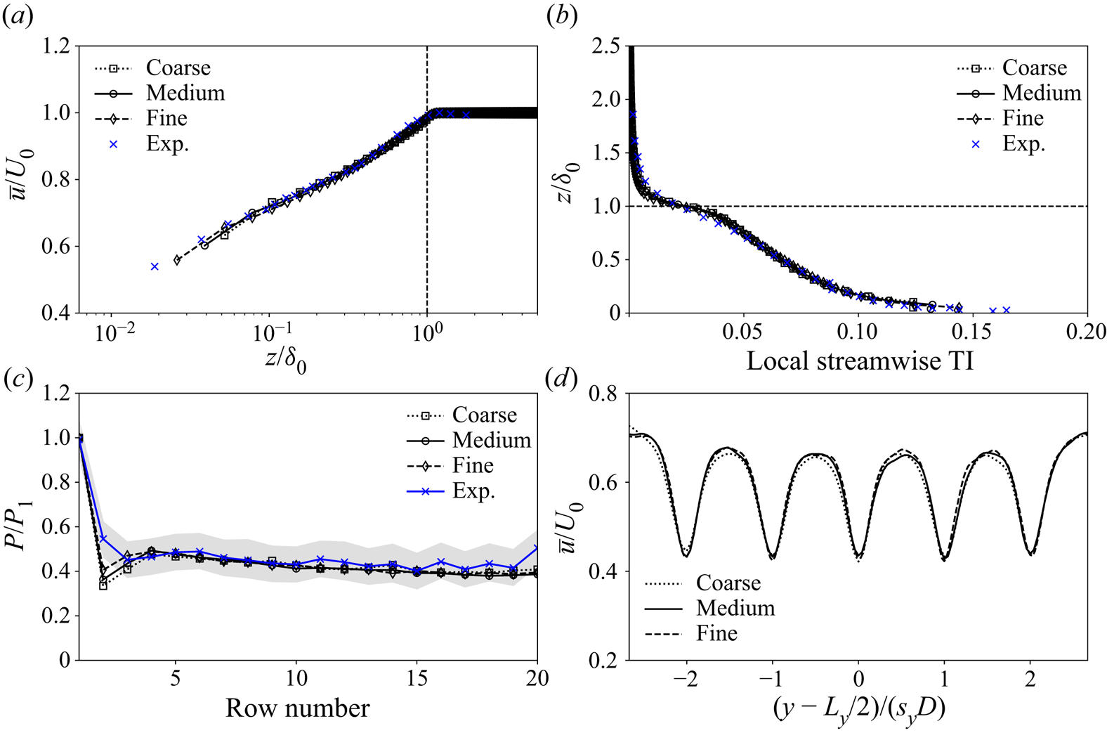
4. LES investigation of wind farm layouts
4.1. Computational set-up
We begin by considering three large finite-length wind farms with different layouts, namely, a fully aligned configuration, a half-staggered configuration and a fully staggered one. The spanwise offset angle between successive turbine rows is  $\alpha =0^\circ,\ 9.46^\circ, 18.43^\circ$ for the aligned, half-staggered and fully staggered configurations, respectively. The considered wind farms consist of 26 rows in the streamwise direction and six turbines in the spanwise direction. The spacing between the turbines is $s_x=7.85$ in the streamwise direction and $s_y=5.23$ in the spanwise direction. The turbine diameter and hub height are $D=100$ and $z_h=100$ m, respectively, and $C^\prime _T=1.33$. The computational domain has dimensions $L_x \times L_y \times L_z = 38\,465 \times 3140 \times 2000$ m and is discretised using $n_x \times n_y \times n_z= 2352 \times 192 \times 129$ points (which is equivalent to a resolution between the medium and fine grids considered in § 3.4). Periodic boundary conditions are used in the streamwise and spanwise directions. The ‘precursor’ part of the domain extends over the first 6280 m ( $L_{ABL}=6280$ m), and the first row of turbines is placed another $6280$ metres downstream ( $L_I=6280$ m). Each simulation is run until a statistically stationary state is reached and the statistics are subsequently gathered over a period corresponding to more than 15 non-dimensional time units (equal to eight hours in physical time). For the boundary layer, we use values similar to Stevens et al. (Reference Stevens, Gayme and Meneveau2014a): friction velocity $u_*=0.45$ m s $^{-1}$, roughness length $z_0=0.1$ m and initial boundary layer height $\delta _0=770$ m.
4.2. Estimation of  $\mathcal {E}$ and $C_M$


Prior to discussing the development of the flow and to be able to compare the model predictions with the LES data, we provide estimations of the entrainment and momentum transfer coefficients using data from the large-eddy simulations. In particular, the entrainment coefficient,  $\mathcal {E}$, is calculated based on its definition and the integral continuity equation (see § 2),
 \begin{equation} \mathcal{E} ={-}\overline{w_\mathcal{E}} / \left(U_0 - U_b \right),\quad \text{with}\ \overline{w_\mathcal{E}}={-}\frac{\mathrm{d}}{\mathrm{d}\kern0.7pt x} \left( {\int _0^\delta \bar{u}}\,\mathrm{d} z \right). \end{equation}
Here, we compute  $\delta$ by considering the location where the tangential turbulent stress is reduced to 5 % of its surface value (Kosović & Curry Reference Kosović and Curry2000). Figure 8 presents the row- and span-averaged values of the entrainment coefficient $\mathcal {E}$ for the different farm arrangements (row-averaging refers to averaging along the streamwise direction, $x$, from $s_xD/2$ upstream of a turbine to $s_xD/2$ downstream). The values of $\mathcal {E}$ are seen to vary with downstream distance but can be considered roughly similar for all arrangements and attain a mean value of $\mathcal {E} \simeq 0.069$. Note that longer averaging times could be beneficial for better statistical convergence with respect to $x$. Nevertheless, the measured values are found to be smaller than those considered by Luzzatto-Fegiz & Caulfield (Reference Luzzatto-Fegiz and Caulfield2018), possibly owing to the definition of $\delta$ or blockage effects in the simulations. Still, our estimates are within the range of values found in the literature (Escudier & Nicoll Reference Escudier and Nicoll1966; Paizis & Schwarz Reference Paizis and Schwarz1975; Cenedese & Adduce Reference Cenedese and Adduce2010). The similarity in the values of $\mathcal {E}$ for the different turbine arrangements may be considered as an indication that the growth of the boundary layer is to a degree independent of the farm layout and that the entrainment model can describe transport processes at the atmospheric layer irrespective of the turbines’ arrangement. Likewise, the momentum transfer coefficient $C_M$ is calculated based on its definition, provided in § 2, and is plotted along with the entrainment coefficient in figure 8. The momentum transfer coefficient decreases slowly with the streamwise distance, attaining a mean value of $C_M \simeq 0.026$, which is in agreement with measurements reported in the literature (Roshko Reference Roshko1993; Chen, Jiang & Nepf Reference Chen, Jiang and Nepf2013; Steiros, Bempedelis & Ding Reference Steiros, Bempedelis and Ding2021). Given the lack of a clear trend for the entrainment coefficient with the streamwise direction, $x$, we assume that both coefficients remain constant throughout the farm. Finally, differences between wind farm layouts appear to be small, less than approximately $10\,\%$, and hence in the model the entrainment and momentum transfer coefficients will both be assumed constant and equal to $\mathcal {E}=0.069$ and $C_M=0.026$, respectively, for all cases.
(a) Row-averaged (RA) values of the entrainment coefficient  $\mathcal {E}$ and (b) momentum transfer coefficient $C_M$ for different farm layouts. The dashed lines denote farm-averaged (FA) values.
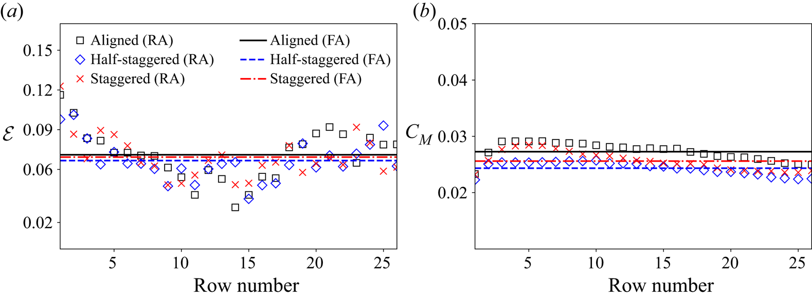
4.3. Flow development
Starting with the flow development, it is important to first examine the streamwise evolution of the boundary layer height,  $\delta$. Figure 9 shows the spanwise-averaged normalised mean streamwise velocity for the case of the aligned wind farm, along with a dashed line that represents the spanwise average of the boundary layer interface. In all subsequent plots, the first row of turbines is used as a reference point for the streamwise distance ( $x_{row 1}=0$).
Contour of spanwise-averaged normalised mean streamwise velocity for the case of the aligned wind farm. The dashed line indicates the spanwise-averaged boundary layer height. The turbines are indicated with short black lines.
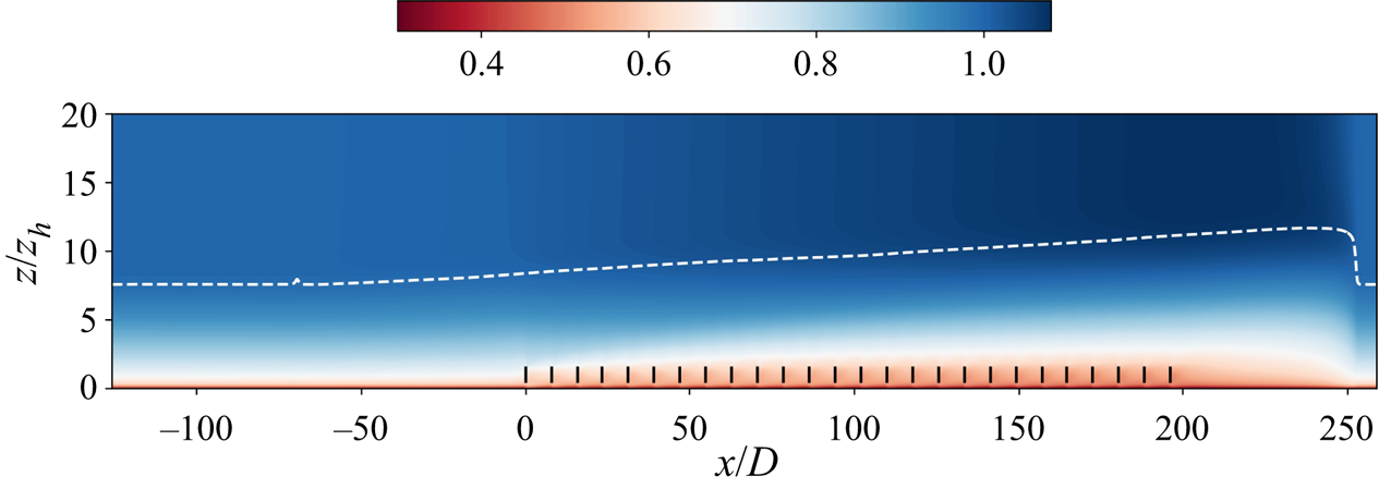
Turning our attention to the effect of different wind farm layouts (aligned, half-staggered, staggered), we present in figure 10 contours of the normalised mean streamwise velocity at hub height  $z_h$. The plotted contours correspond to the entrance region of the farm, and in particular to the first 10 rows of turbines. In the case of the aligned farm, high-velocity streaks may be observed between the turbines. Downstream turbines operate entirely within the wake of upstream turbines, with large velocity deficits established immediately after the first row. In the case of the staggered farms, the wakes are allowed more space to recover and interfere less with the downstream turbines. Hence, the velocity field is considerably more homogeneous along the spanwise direction.
Contours of normalised mean streamwise velocity at hub height  $z_h$ for the three wind farm layouts considered herein: (a) aligned, (b) half-staggered and (c) fully staggered.
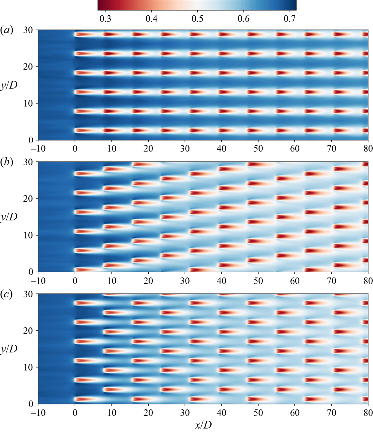
Next, we integrate the streamwise velocity according to our entrainment model layer approach to obtain the characteristic bulk velocities  $U_f$ and $U_b$, and plot them in figure 11. Here, $U_b$ is shown to be unaffected by the farm layout, whereas $U_f$ is larger for the aligned farm than for the staggered farms, owing to the streamwise streaks of high velocity that persist between the turbines. The trends predicted by the model are in agreement with the LES data – more so for the staggered cases, which display higher levels of spanwise homogeneity – but smaller in magnitude. The streamwise evolution of the boundary layer for different farm layouts is also presented in figure 11. The farm layout is shown to have only a small effect on the growth of the atmospheric boundary layer. Here, the model predictions are in good agreement with the LES data. This is because the boundary layer growth rate is directly proportional to the entrainment coefficient $\mathcal {E}$, which was extracted from the LES data. The good overall agreement (both qualitative and quantitative) between the model and the LES data confirms the ability of the model to capture the mean flow and boundary layer height evolution.
(a) Spanwise-averaged normalised characteristic velocities and (b) boundary layer height for different farm arrangements. Also plotted are the model predictions.
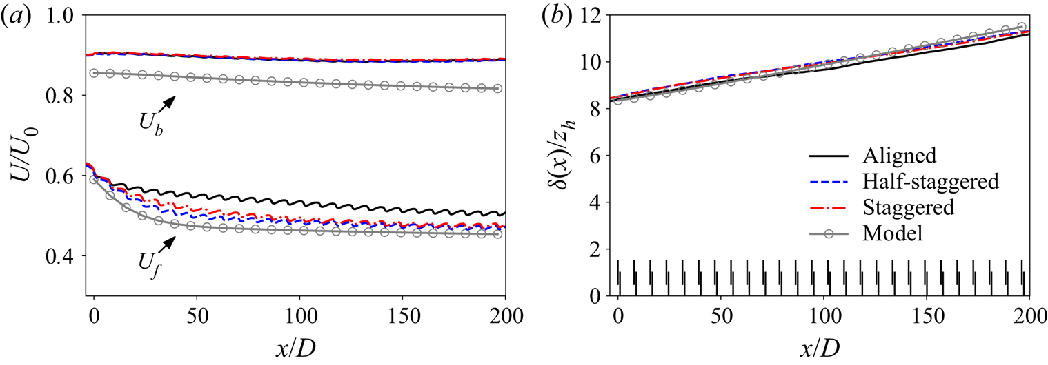
4.4. Spatial evolution of kinetic energy and wind power generation
The evolution of mean-flow kinetic energy within the wind farm can be expressed as
 \begin{equation} \underbrace{\overline{u_j} \frac{\partial \bar{K}}{\partial x_j}}_{{advection}} + \underbrace{\frac{\partial}{\partial x_j} \left( \overline{u_i} \left(\overline{u'_{i} u'_{j}} +\overline{\tau_{ij}} \right) \right)}_{{turbulent\ MKE\ flux}} + \underbrace{\overline{u_i} \frac{\partial}{\partial x_i} \left(\frac{\bar{p}}{\rho} \right)}_{{pressure\ work}} = \underbrace{\left (\overline{u'_{i} u'_{j}}+\overline{\tau_{ij}} \right) \frac{\partial \overline{u_i}}{\partial x_{j}}}_{{TKE\ production}} + \underbrace{ \overline{u_i} \frac{\overline{f_i^T}}{\rho}}_{\substack{{turbine}\\ {power}}}. \end{equation}
Equation (4.2) has been used in a number of past works (Cal et al. Reference Cal, Lebrón, Castillo, Kang and Meneveau2010; Calaf et al. Reference Calaf, Meneveau and Meyers2010; Newman et al. Reference Newman, Drew and Castillo2014; VerHulst & Meneveau Reference VerHulst and Meneveau2014; Cortina, Calaf & Cal Reference Cortina, Calaf and Cal2016; Allaerts & Meyers Reference Allaerts and Meyers2017; Andersen et al. Reference Andersen, Sørensen and Mikkelsen2017; Cortina et al. Reference Cortina, Sharma, Torres and Calaf2020) to illustrate the mechanisms that are responsible for transporting the energy of the wind to the turbines’ location and thereby contributing to wake recovery and farm performance. Traditionally, MKE transport has been studied in the context of infinite-length wind farms (e.g. Calaf et al. Reference Calaf, Meneveau and Meyers2010; Cortina et al. Reference Cortina, Calaf and Cal2016). In finite-length wind farms, the contributions of each transport mechanism are expected to differ as we move to different locations within the farm; advection dominates in the initial rows, whereas in downstream rows of large (or infinite) wind farms, energy is transported vertically from above the farm, via turbulence. Additionally, the layout of the farm is also expected to have an effect on the role of each energy transport mechanism. Here, we will be focusing on the evolution of the terms that are primarily responsible for transporting energy from the atmospheric flow into the wind farm, i.e. advection and turbulent transport (Andersen et al. Reference Andersen, Sørensen and Mikkelsen2017). Similar to the discussion in § 2, we consider control volumes that surround each row (from  $x=-s_xD/2$ to $x=s_xD/2$ upstream and downstream of each turbine row, respectively) and extend vertically from the ground to the top of the turbines $(0 < z < z_h + D/2)$. We therefore obtain
 \begin{equation} A+\varPhi-\varepsilon-P_{WT}=R, \end{equation}
where  $A$ is the advection term, $\varPhi$ is the MKE turbulent flux term, $\varepsilon$ is the turbulence kinetic energy (TKE) production term, $P_{WT}$ is the power extracted by the wind turbines and $R$ is a remainder term corresponding to pressure work and the MKE budget residual (due to errors in numerical integration, statistical convergence etc.), which was confirmed to be comparably small.
Figure 12 plots the control volume integrated advection of MKE,  $A$, as a function of the turbine row number along with the predictions of the entrainment model. Note that both the LES data and model predictions have been normalised by the reference velocity, $U_0$, and the reference length scale, $D$. The rotor diameter $D$ is used as the quantities of interest are integrated in the wind farm layer. Starting with the magnitude of the MKE advection term, we note that it decreases as we move deeper into the farm. Moreover, it is found to be larger for the aligned farm (except for the first few rows), which can be attributed to the streamwise high-velocity streaks (see figure 10). In other words, the staggered arrangements are found to be more efficient at extracting the kinetic energy available at their level. Comparing the LES results with our entrainment-based model, we find that MKE advection is not well predicted in the case of the aligned wind farm, owing to the lack of flow homogeneity along the spanwise direction. Nonetheless, the model predictions are in good agreement with the LES results for both staggered farms.
(a) MKE advection and (b) turbulent transport as a function of turbine row for different farm layouts. Also shown are the model predictions.

The contributions of the vertical turbulent transport term,  $\varPhi$, are measured via the top surface of the control volumes, i.e. at the turbine top level $z_h + D/2$. Figure 12 shows that the normalised vertical turbulent transport is larger for the staggered arrangements, with a peak observed around the fifth row, before slowly decreasing with downstream distance. The model predictions are shown to be in good agreement with the LES results (this is also true for the control volume integrated values of $\varPhi$, which are not plotted in figure 12 for clarity). As advection is no longer contributing beyond the first 10 rows, the mechanism that is responsible for transporting energy to the turbines’ location is turbulence. This is in agreement with observations of past works (e.g. Cortina et al. Reference Cortina, Sharma, Torres and Calaf2020), and therefore it can be concluded that in the deep array region, power extracted by the turbines is replenished by vertical turbulent transports.
Next, figure 13 shows the evolution of the control volume integrated TKE production term,  $\varepsilon$, within the wind farm. In particular, it is shown that TKE production is larger for the fully aligned farm layout, though differences may be observed between the staggered arrangements as well. More specifically, the half-staggered arrangement presents a slightly more uniform evolution in the initial rows. This is because more turbines operate within a ‘cleaner’ wind field. We note that the different levels of TKE production are associated with different levels of turbulent kinetic energy. This is particularly true in the case of aligned wind farms, where turbines operate within a stronger turbulence field. A closer look at the spanwise-averaged TKE production vertical profiles, shown in figure 14, reveals that the equilibrium that is expected to be established in the deep-array wind farm region can be approximately achieved only after the fifteenth row of turbines. At that point, turbulent MKE dissipation tends to $u_{*hi}^3/(\kappa z)$, where $u_{*hi}$ is the wind farm friction velocity (Frandsen Reference Frandsen1992). This is the limit proposed by Calaf et al. (Reference Calaf, Meneveau and Meyers2010) and suggests a fully developed wind farm boundary layer. It is worth noting that such conditions are not fully established even after the twentieth row of turbines.
TKE production as a function of turbine row for different farm layouts.
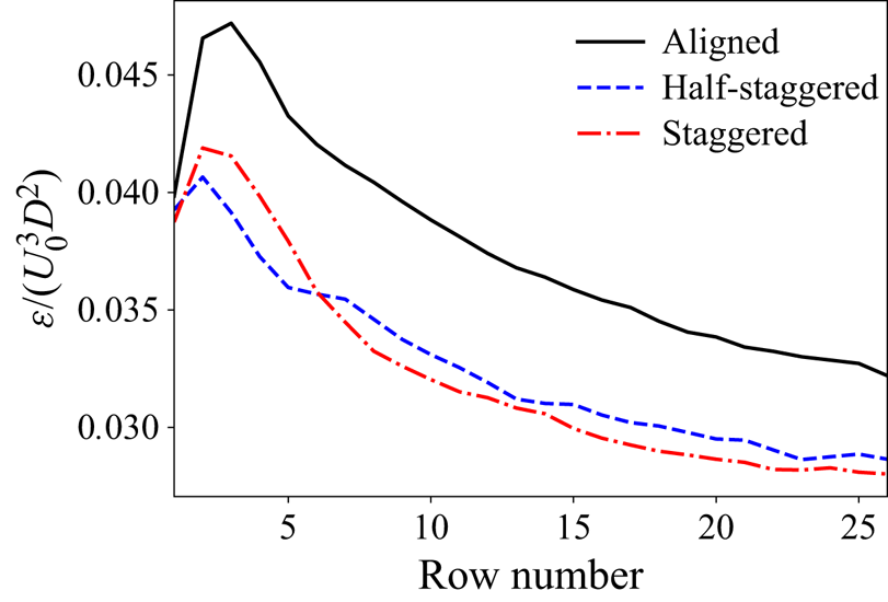
Spanwise-averaged vertical profiles of turbulent MKE dissipation for different farm layouts at different positions within the farm. Denoted with vertical dash–dotted lines are the turbine top and bottom heights. Markers are shown every two  $z$-grid nodes.
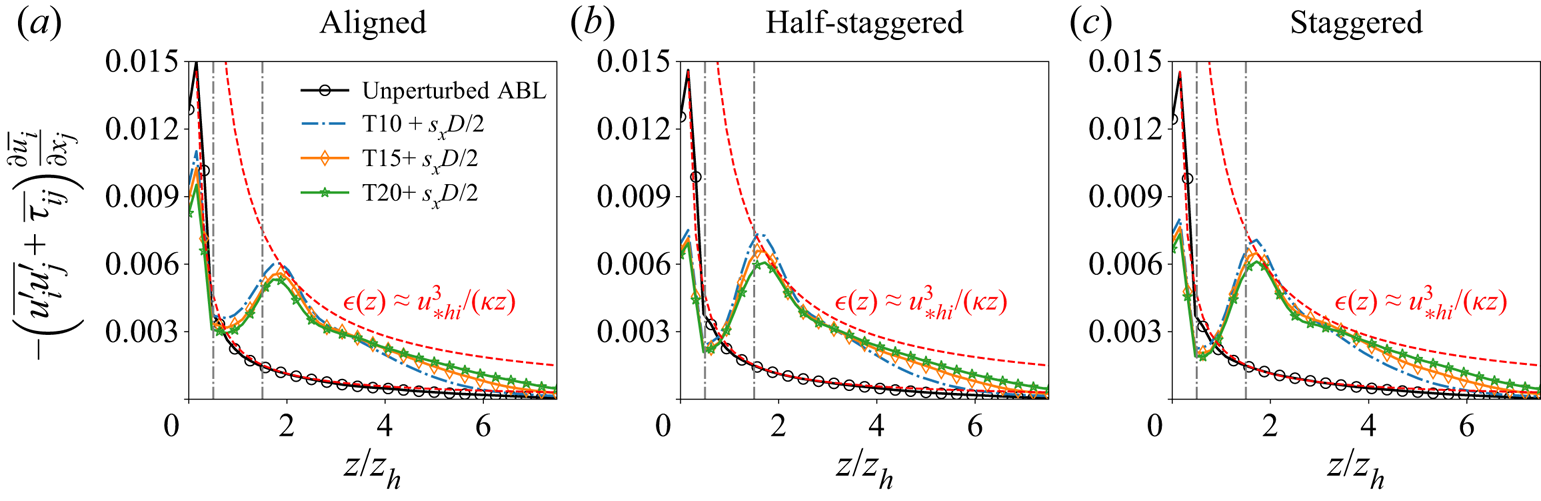
Figure 15 shows the LES data for the power of the wind turbines normalised by the power of the first row, along with the predictions of the entrainment-based model. In the case of the aligned wind farm, the ‘infinite’ power limit is established shortly after the wind farm entrance. However, the power decreases more gradually in the staggered cases, with a peak value occurring in the second row of turbines, which is attributed to blockage effects induced by the first row of turbines and results in a local acceleration of the flow in the region between the turbines. Our model predicts a decrease in power that is in accordance with the power measured in staggered wind farms. However, the power deficit predicted by the model is larger; this is related to the underprediction of the bulk velocities (see figure 11) and can also be, to a degree, attributed to blockage effects due to the relatively confined simulation domain ( $L_z=2$ km).
LES predictions of the normalised power output for different farm arrangements along with the model predictions.

4.5. Turbine spacing, operating regime and inflow conditions
Before concluding our study, we shall examine the effects of turbine spacing, operating point (thrust coefficient) and incoming atmospheric boundary layer height. To this end, we first consider two fully staggered wind farms of 26 rows each with different turbine spacings: a densely populated farm ( $s_x=5.23$, $s_y=3.49$) and a thinly populated farm ( $s_x=11.78$, $s_y=7.85$). In each case, the domain size is modified accordingly to accommodate the wind farms of different lengths. All other simulation parameters remain as described in § 4.1. Figure 16(a) shows the power output of the fully staggered wind farms with different turbine spacings. As expected, a smaller spacing between turbines leads to a decrease in power output. The model is able to capture the effects of different turbine spacings but, as previously discussed, with a slight overprediction of the power deficit when compared to the LES data. This trend is more pronounced for small spacings, suggesting that the model seems to be more accurate when the turbine wakes are interacting less. It should be noted that the coefficient of variation (standard deviation divided by the mean) of the empirical coefficients $\mathcal {E}$ and $C_M$ in the simulations with different array spacings is smaller than 10 % (8.04 % and 8.46 %, respectively) while both coefficients were assumed constant in the model.
(a) Normalised power output for different turbine spacings, (b) thrust coefficients and (c) inflow conditions. LES numerical data are represented by symbols and the model predictions by lines.

Next, we consider changes in the operating point of the turbines, i.e. in the thrust coefficient. Two scenarios are considered: one where the turbines operate with  $C_T=0.75$ ( $C^\prime _T=1.33$) and one where $C_T=0.89$ ( $C^\prime _T=2$), which corresponds to the Betz limit for maximum power extraction. As seen in figure 16(b), the turbines in downstream rows produce less power relative to the output of the first row in the high thrust coefficient case. The model captures the trends in relative power for different thrust coefficients, but overestimates the power deficit in the high-thrust-coefficient case, i.e. $C^\prime _T=2$. This may be attributed to the gradual emergence of pressure effects (which are neglected in the present analysis) when turbines operate at relatively high induction factors (Steiros & Hultmark Reference Steiros and Hultmark2018; Bempedelis & Steiros Reference Bempedelis and Steiros2022; Steiros, Bempedelis & Cicolin Reference Steiros, Bempedelis and Cicolin2022).
Finally, a simulation of a fully staggered wind farm is performed under different inflow conditions, i.e. considering a thin boundary layer where  $\delta _0/z_h=2.5$. Figure 16(c) shows that the height of the inflow boundary layer has a limited impact on the power output, with only a small decrease with decreasing boundary layer thickness. The results are in agreement with the observations of Allaerts & Meyers (Reference Allaerts and Meyers2017) for wind farms in conventionally neutral atmospheric conditions. As already discussed in § 2, the model is also shown to be able to reproduce the small decrease in power output when the atmospheric boundary layer thickness is decreased.
5. Summary and conclusions
In this work, we have proposed a model for the prediction of the flow within finite-length wind farms. The model is an extension of the work of Luzzatto-Fegiz & Caulfield (Reference Luzzatto-Fegiz and Caulfield2018) for ‘infinite-length’ farms, and makes use of the entrainment hypothesis to relate the growth of the atmospheric boundary layer to the flow and performance of the wind farm. The model approximates the flow field by dividing it into three regions (wind farm layer, by-pass layer and outer layer), with exchanges taking place at their interfaces. Our extension assumes dependence of flow quantities on the streamwise distance from the farm entrance, and may thus be used to describe both the developing and the fully developed flow regions in large wind plants. Estimations of quantities of interest for wind farm performance, such as the power output of the farm or the exchanges between the wind farm and the atmospheric boundary layer, may also be obtained. It was shown that for very large wind farms, the predictions of the newly developed model asymptotically trend to the ‘infinite-farm’ limit values of the model of Luzzatto-Fegiz & Caulfield (Reference Luzzatto-Fegiz and Caulfield2018). However, it was found that the ‘infinite-farm’ values are only approached in rows deep in the farm and in the case of very large wind farms (typically consisting of more than 15 rows).
To validate our model, we conducted a series of large-eddy simulations for a neutral atmospheric boundary layer developing over large wind farms and examined the performance and flow characteristics of farms with different turbine arrangements and inflow conditions. The LES data were also used to assist the assessment of the performance of our entrainment-based model. Measurements of the entrainment and momentum transfer coefficients at the boundary layer and farm layer interfaces, respectively, showed that they are only little affected by the wind farm layout. The boundary layer height and characteristic velocities above the wind farm layer were also found to not be significantly affected by the farm layout. However, wind farms of different layouts make different usage of the energy that is available to them, with staggered arrangements producing more power, in both the entrance rows and the deep-array region. Looking at the wind farm MKE evolution, the aligned wind farm was found to extract less power from the available resource, while also displaying increased amounts of TKE production. The turbulent transport of MKE, however, was found to evolve in a non-monotonic fashion, with its peak occurring within the developing wind farm region. The model predictions for the key flow variables and farm performance, as well as for the mechanisms of energy transport from the atmospheric wind, were found to be in good agreement with the LES data throughout the wind farm, particularly for staggered arrangements, where the spanwise homogeneity assumption of the model is more pertinent.
In future studies, we plan to carry out more simulations and further investigate the effects of turbine spacing and atmospheric conditions and their implications for the energy transport and entrainment characteristics. Together with the principles regarding the parametrisation of the empirical coefficients put forth by Luzzatto-Fegiz & Caulfield (Reference Luzzatto-Fegiz and Caulfield2018), this will pave the way for application of the finite-length entrainment model in non-neutral conditions. Moreover, considerations of the most prominent turbulent structures and their length scales may be used to promote wind farm layout designs that enable increased momentum exchanges and lead to increased overall wind farm power output.
Funding
The authors would like to thank the Engineering and Physical Sciences Research Council for the computational time made available on the UK supercomputing facility ARCHER2 via the UK Turbulence Consortium (EP/R029326/1) and via an ARCHER2 Pioneer Project. Time was also made available on Isambard via an EPSRC Tier 2 project. N.B. and S.L. would like to acknowledge the support of EPSRC grant no. EP/V000942/1. G.D. would like to acknowledge funding from the U.S. Department of Energy. This work was authored in part by the National Renewable Energy Laboratory, operated by the Alliance for Sustainable Energy, LLC, for the U.S. Department of Energy (DOE) under contract no. DE-AC36-08GO28308. Funding was provided by the U.S. DOE Office of Energy Efficiency and Renewable Energy Wind Energy Technologies Office. The views expressed in the article do not necessarily represent the views of the DOE or the U.S. Government. The U.S. Government retains and the publisher, by accepting the article for publication, acknowledges that the U.S. Government retains a non-exclusive, paid-up, irrevocable, worldwide license to publish or reproduce the published form of this work, or allow others to do so, for U.S. Government purposes.
Declaration of interests
The authors report no conflict of interest.
Appendix A. Approximate wind farm layer momentum magnitude
In this section, we provide a derivation for the approximation
 \begin{equation} \int _0^{h_f} \bar{u}^2\,\mathrm{d}z \approx h_f U_f^2(x). \end{equation}
We start by using the identity  $(\bar {u}-U_f)^2=\bar {u}^2-2\bar {u}U_f+U_f^2$ to obtain
 \begin{equation} \int _0^{h_f} \bar{u}^2\,\mathrm{d} z = \int_0^{h_f} (\bar{u}-U_f)^2\,\mathrm{d} z + \int _0^{h_f} 2\bar{u}U_f\,\mathrm{d} z - \int _0^{h_f} U_f^2\,\mathrm{d}z. \end{equation}
Since  $U_f$ is the integral layer velocity, it is independent of $z$ and therefore can be taken out of the integral, yielding
 \begin{align} \int _0^{h_f} \bar{u}^2\,\mathrm{d} z &= \int _0^{h_f} (\bar{u}-U_f)^2\,\mathrm{d} z + 2 U_f \int _0^{h_f} \bar{u}\,\mathrm{d} z - h_f U_f^2 \nonumber\\ &= \int _0^{h_f} (\bar{u}-U_f)^2\,\mathrm{d} z + 2 h_f U_f^2 - h_f U_f^2 \nonumber\\ &= \int _0^{h_f} (\bar{u}-U_f)^2\,\mathrm{d} z +h_f U_f^2 \approx h_f U_f^2. \end{align}
The last step involves the assumption  $\int _0^{h_f} (\bar {u}-U_f )^2\, \mathrm {d} z \ll \int _0^{h_f} U_f^2 \,\mathrm {d} z$. Physically, this may be interpreted as assuming the turbine wakes to follow a top-hat profile, similar to many analytical wind turbine wake models (Jensen Reference Jensen1983; Frandsen et al. Reference Frandsen, Barthelmie, Pryor, Rathmann, Larsen, Højstrup and Thøgersen2006; Bempedelis & Steiros Reference Bempedelis and Steiros2022).
Appendix B. Entrainment model sensitivity analysis
Similar to Luzzatto-Fegiz & Caulfield (Reference Luzzatto-Fegiz and Caulfield2018), we consider the effect of varying  $\mathcal {E}$ and $C_M$ by ${\pm }20\,\%$. Figure 17 shows the model predictions, where the solid lines correspond to the reference values (see § 2) and the shaded region to the effect of a ${\pm }20\,\%$ change in $\mathcal {E}$ and $C_M$. The by-pass characteristic velocity, relative turbine power output and MKE advection show little sensitivity to the changes, in contrast to the wind farm characteristic velocity, absolute power output and turbulent transport of MKE at the farm layer interface. This means that different values of $\mathcal {E}$ and $C_M$ affect the wind farm power production, as observed by Luzzatto-Fegiz & Caulfield (Reference Luzzatto-Fegiz and Caulfield2018), but that the flow develops in a qualitatively similar manner. Lastly, the boundary layer is shown to grow at a different rate as it moves deeper into the wind farm. Overall, the expected behaviour is observed, where larger values for the entrainment and momentum transfer coefficients imply larger transfers and replenishment of energy, and therefore increased farm power and faster boundary layer growth.
Model predictions for a  ${\pm }20\,\%$ change in $\mathcal {E}$ and $C_M$.
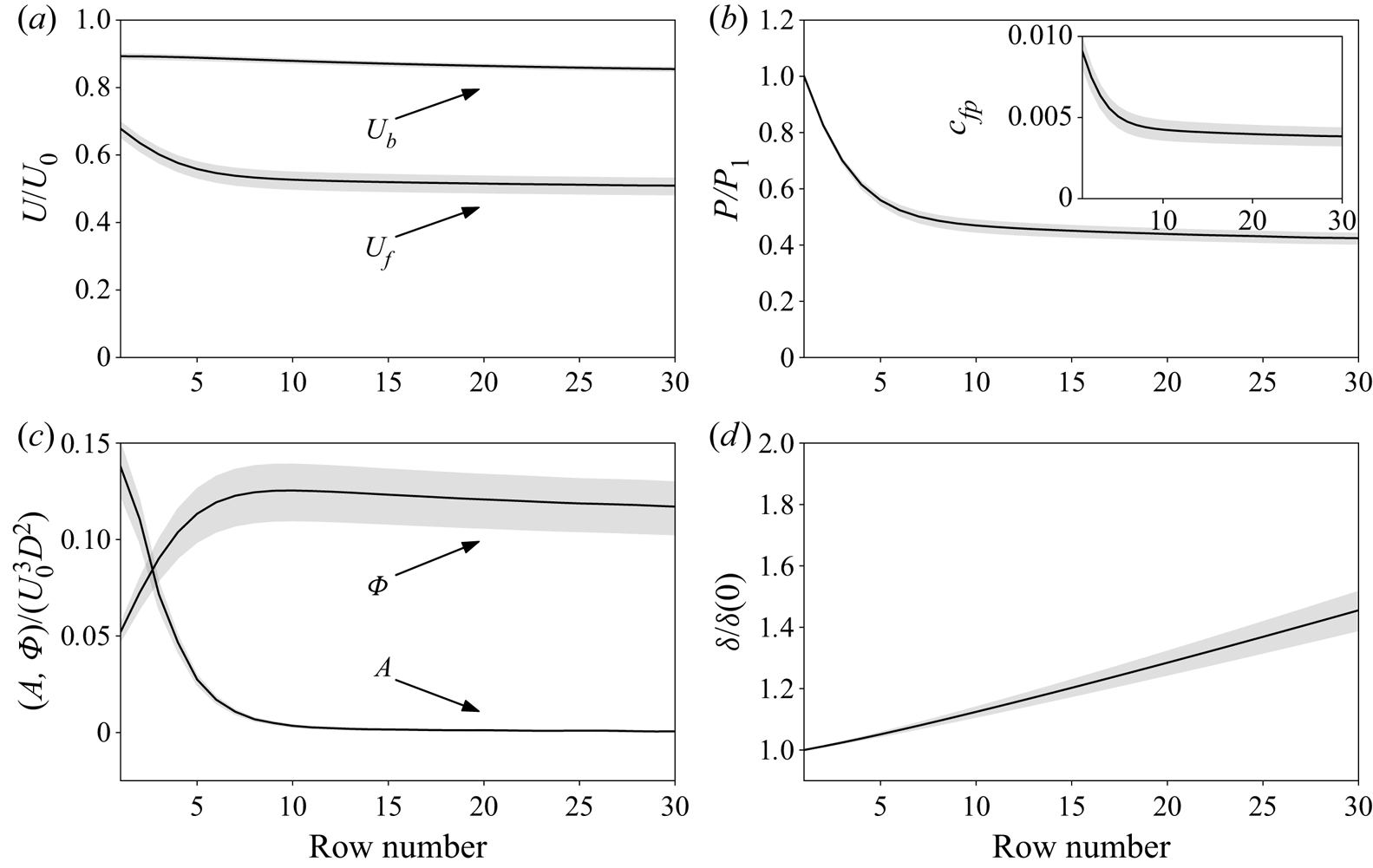


 Open access