


1 Introduction
Streamwise time-averaged vortices, known as secondary currents (SCs), can often be observed in straight open-channel flows (OCFs), where they are generated near the sidewalls due to the effects of turbulence anisotropy (e.g. Nezu & Nakagawa Reference Nezu and Nakagawa1993). SCs can also emerge within the flow cross-section if the bed is spanwise heterogeneous (e.g. Mejia-Alvarez & Christensen Reference Mejia-Alvarez and Christensen2013; Barros & Christensen Reference Barros and Christensen2014, Reference Barros and Christensen2019). Such heterogeneities can be associated with changes in bed topography (variations in bed elevation comparable to the flow outer scale, i.e. the flow depth in OCFs) and/or in bed surface roughness. As an example, mobile-bed open channels may be characterised by the natural appearance of spanwise-periodic streamwise sand or gravel ridges (e.g. Colombini & Parker Reference Colombini and Parker1995), continuous protrusions along the flow that generally feature different surface roughness from the rest of the bed.
A number of experimental and numerical studies have explored open-channel, closed-channel and boundary-layer flows over streamwise ridges with different cross-sectional shapes (e.g. Nezu & Nakagawa Reference Nezu and Nakagawa1993; Wang & Cheng Reference Wang and Cheng2006; Vanderwel & Ganapathisubramani Reference Vanderwel and Ganapathisubramani2015; Hwang & Lee Reference Hwang and Lee2018; Medjnoun, Vanderwel & Ganapathisubramani Reference Medjnoun, Vanderwel and Ganapathisubramani2018; Vanderwel et al. Reference Vanderwel, Stroh, Kriegseis, Frohnapfel and Ganapathisubramani2019; Zampiron et al. Reference Zampiron, Nikora, Cameron, Patella, Valentini and Stewart2020), alternating streamwise strips of different surface roughness (e.g. Nezu & Nakagawa Reference Nezu and Nakagawa1993; Wang & Cheng Reference Wang and Cheng2006; Willingham et al. Reference Willingham, Anderson, Christensen and Barros2014; Anderson et al. Reference Anderson, Barros, Christensen and Awasthi2015; Bai, Kevin & Monty Reference Bai, Kevin and Monty2018; Chung, Monty & Hutchins Reference Chung, Monty and Hutchins2018; Wangsawijaya et al. Reference Wangsawijaya, de Silva, Baidya, Chung, Marusic and Hutchins2018) and converging/diverging riblet patterns (e.g. Nugroho, Hutchins & Monty Reference Nugroho, Hutchins and Monty2013; Kevin et al. Reference Kevin, Bai, Pathikonda, Nugroho, Barros, Christensen and Hutchins2017; Kevin & Hutchins Reference Kevin and Hutchins2019). The majority of these works address heterogeneities in bed topography and surface roughness separately, as the examined surfaces mostly consist of ridges featuring the same surface roughness as the underlying bed (i.e. smooth ridges on a smooth wall or rough ridges on a rough wall) or variations in surface roughness without altering the bed topography.
Spanwise bed heterogeneities have been mainly found to generate SCs with upflows and associated low-momentum pathways located at ridges, at strips of lower surface roughness and above converging riblets. However, studying the effects of rows of streamwise-aligned pyramidal elements in closed-channel flow at different spanwise spacings, Yang & Anderson (Reference Yang and Anderson2018) observed a reversal in the rotation direction of the SCs at particular spacings. Their results showed that, for transverse spacings of the pyramid rows greater than the channel half-height, the rotation direction of the cells switched such that downflow regions and associated high-momentum pathways became aligned with the roughness elements. Although the reason for such an effect has not been found yet, the roughness pattern seen by Yang & Anderson (Reference Yang and Anderson2018) may indeed represent an intermediate case between topographical and surface roughness heterogeneities. Hwang & Lee (Reference Hwang and Lee2018) proposed that the rotation direction of the SCs is mainly driven by the turbulent transport of turbulent kinetic energy, which may significantly depend on the flow conditions and the characteristics of the bed heterogeneity. Downflows above the ridges were also found for ridge widths comparable to the flow outer scale (Wang & Cheng Reference Wang and Cheng2006; Hwang & Lee Reference Hwang and Lee2018) due to the appearance of additional SCs, similar to those observed by Vanderwel & Ganapathisubramani (Reference Vanderwel and Ganapathisubramani2015) for large ridge spacings relative to the boundary-layer thickness. The issue of the rotational direction of the SC cells has been recently explored in Anderson (Reference Anderson2019). The author showed that, even at the same spacing, there is a possibility of the occasional change in the direction of cell rotation that is chaotic in nature. This finding opens a new avenue for exploring secondary currents and their stability. Despite the differences in SC rotation direction, all studied surface types have been found to generate arrays of SC cells with sizes that scale with the characteristic transverse length of the roughness heterogeneity. Yang & Anderson (Reference Yang and Anderson2018) reported that, for transverse ridge spacings sufficiently smaller than the channel half-height, the induced SCs do not occupy the entire flow domain but are instead confined to the near-bed region. SCs, regardless of their origin, contribute to momentum exchange and mixing. They modify turbulence structure, sediment transport and hydraulic resistance, and thus have to be accounted for in river modelling and management systems.
SCs share a number of similarities with very-large-scale motions (VLSMs) or ‘superstructures’ (e.g. Kim & Adrian Reference Kim and Adrian1999; Hutchins & Marusic Reference Hutchins and Marusic2007; Monty et al. Reference Monty, Hutchin, Ng, Marusic and Chong2009). They both appear as large counter-rotating streamwise vortices introducing elongated streaks of alternating high- and low-momentum fluid. However, while SCs are a feature of the time-averaged velocity field, VLSMs meander laterally in time and therefore, within the framework of the Reynolds averaging, represent turbulence (e.g. Adrian & Marusic Reference Adrian and Marusic2012). Early observations consistent with the existence of very long coherent structures in the streamwise direction date back to some early works (e.g. Bullock, Cooper & Abernathy Reference Bullock, Cooper and Abernathy1978; Perry, Henbest & Chong Reference Perry, Henbest and Chong1986; Kim, Moin & Moser Reference Kim, Moin and Moser1987). However, the existence and scaling properties of VLSMs were not systematically identified until the study of Kim & Adrian (Reference Kim and Adrian1999), who characterised the long-wavelength structures (12–14 pipe radii) in pipe flows using pre-multiplied velocity spectra. VLSMs have now been extensively studied in the context of smooth-wall pipe, closed-channel and boundary-layer flows. Finding a good match between pipe and conduit flows, Monty et al. (Reference Monty, Hutchin, Ng, Marusic and Chong2009) proposed a power-law-type relationship describing the dependence of the VLSM streamwise wavelength as a function of the elevation from the bed. One important difference between the structures found in pipes and conduits and those in boundary layers is that, for boundary-layer flows, the VLSMs appear to be confined to the logarithmic layer, whereas in pipes and conduits the structures extend further into the outer flow. For this reason the term ‘superstructure’ (Hutchins & Marusic Reference Hutchins and Marusic2007) is often reserved for boundary-layer flows. In rough-bed OCFs, VLSMs have only recently been identified (Cameron, Nikora & Stewart Reference Cameron, Nikora and Stewart2017) with lengths ( ${\approx}10{-}40$ flow depths) often much longer than for pipes, conduits and boundary layers. Additionally, the length of VLSMs in OCFs has been found to depend on the roughness type, the flow width-to-depth ratio and the flow depth-to-roughness-height ratio. The origin of the VLSMs or superstructures is not yet clear, with Kim & Adrian (Reference Kim and Adrian1999) proposing that they result from the spatial alignment of shorter hairpin packets, while Hwang & Cossu (Reference Hwang and Cossu2010) considered the structures to form directly and self-sustain from a large-scale flow instability mechanism.
Given the similarities between SCs and VLSMs, it is possible that they interact with each other in some way and/or have similar generation mechanisms. Adrian & Marusic (Reference Adrian and Marusic2012) speculate that, in straight OCFs, VLSMs may in fact be some kind of instantaneous manifestation of SCs, while Nugroho et al. (Reference Nugroho, Hutchins and Monty2013) and Kevin et al. (Reference Kevin, Bai, Pathikonda, Nugroho, Barros, Christensen and Hutchins2017) suggested that roughness-induced SCs could be the result of the preferential alignment of VLSMs imposed by the bed heterogeneities. Streamwise ridges represent a convenient example of spanwise bed heterogeneity to explore potential interrelations between SCs and VLSMs, as the SCs can be systematically varied by changing the inter-ridge spacing. Despite a number of studies on the flow over streamwise ridges, the potential role of VLSMs in such flows has generally been overlooked. There are very few studies characterising the velocity spectra for flows over spanwise-heterogeneous roughness. Notable exceptions are the two boundary-layer studies of Nugroho et al. (Reference Nugroho, Hutchins and Monty2013) using riblet roughness and Wangsawijaya et al. (Reference Wangsawijaya, de Silva, Baidya, Chung, Marusic and Hutchins2018) using alternating smooth and rough strips, and the work of Awasthi & Anderson (Reference Awasthi and Anderson2018) on multi-scale roughness in closed-channel flow. All these studies report significant differences between their measured spectra and those obtained for smooth walls. The data currently available, however, are still insufficient to generalise the observed behaviour.
Additional motivation for this study comes from our preliminary measurements of the friction factor ( $f_{H}$) for fully rough beds covered with smooth streamwise-oriented ridges (Zampiron et al. Reference Zampiron, Nikora, Cameron, Patella, Valentini and Stewart2020). We found that, at ridge spacings of ${\approx}1.6$ flow depths ( $H$), the friction factor is maximised, while at spacings smaller than ${\approx}0.7H$, it is reduced below that predicted without accounting for transverse momentum fluxes. These effects are clear in figure 1(a), which shows the ratio of measured $f_{H}$ to an estimated friction factor ( $f_{EST}$) obtained following a conventional procedure known as the ‘channel divided method’ (e.g. Chow Reference Chow1959). Using this method, the channel cross-section is partitioned into ‘ridge’ regions with a hydraulically smooth surface and rough surface regions between the ridges. Appropriate friction factors and part of the total flow cross-sectional area are assigned to each region. The friction factor of the combined regions ( $f_{EST}$) is then calculated satisfying the mass conservation equation. The obtained value represents an idealised friction factor without accounting for potential effects of mean momentum exchange between the sub-regions due to, for example, SCs. The ratio $f_{H}/f_{EST}$ therefore illustrates the potential influence of SCs on the friction factor.
The objective of this study is to explore SCs and VLSMs in OCFs over hydraulically rough beds covered by streamwise ridges, for a range of ridge spacings. The structure of the paper is as follows. In § 2 the open-channel flume, the stereoscopic particle image velocimetry (PIV) measurement system and the hydraulic conditions used in the experiments are described. In § 3 we report time-averaged velocity statistics, double-averaged (in time and space) velocity and stress distributions, contours of instantaneous streamwise velocity, velocity spectra and co-spectra, two-point correlation functions and the proper orthogonal decomposition of the velocity field. Finally in § 4 the main findings of the study are summarised and discussed.
(a) Normalised friction factor  $f_{H}/f_{EST}$ as a function of the relative ridge spacing $s/H$; (b) illustration of maximum ( $H$) and mean ( $\bar{H}$) flow depths and ridge spacing ( $s$); and (c) stereoscopic PIV configuration.

2 Experimental set-up
2.1 Open-channel facility, bed roughness and hydraulic conditions
Experiments were conducted in the ‘RS’ flume in the Fluid Mechanics Laboratory of the University of Aberdeen (e.g. Stewart et al. Reference Stewart, Cameron, Nikora, Zampiron and Marusic2019). The facility consists of a recirculating open-channel flume with adjustable slope. The channel is 0.4 m wide with a working length of 10.75 m and glass sidewalls 250 mm high. Flow uniformity is assessed using a series of digital point gauges positioned along the channel. The point gauges are also used to measure flow depth by differencing measured bed and water surface elevations. Flow rate is controlled by adjusting the speed of a centrifugal pump and measured by an electromagnetic flowmeter. A series of guide vanes and honeycomb panels in the flume entrance tank secure a flow that is uniformly distributed and free of large-scale turbulence as it enters the channel.
Experimental conditions:  $s$ is ridge spacing; $H$ is maximum flow depth; $b$ is ridge width; $h$ is ridge height; $\bar{H}$ is mean flow depth (figure 1); $Q$ is flow rate; $U=Q/(B\bar{H})$ is bulk flow velocity, with $B$ the channel width; $u_{\ast }=\sqrt{g\bar{H}S_{b}}$ is shear velocity, with $g$ the gravitational acceleration and $S_{b}$ the bed slope; $Re=U\bar{H}/\unicode[STIX]{x1D708}$ is bulk Reynolds number, with $\unicode[STIX]{x1D708}$ the kinematic viscosity; $H^{+}=u_{\ast }\bar{H}/\unicode[STIX]{x1D708}$ is friction Reynolds number; $Fr=U/\sqrt{g\bar{H}}$ is Froude number; and $f_{H}=8u_{\ast }^{2}/U^{2}$ is the Darcy–Weisbach friction factor.

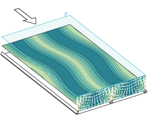
Streamwise ridges were attached to the bed of the flume using a hook-and-loop fastener system to allow easy adjustment of the spacing between adjacent ridges. The bed of the flume was completely covered by a single fabric sheet constituting the hook component, with the hooks of height  $\unicode[STIX]{x1D6E5}\approx 1.1~\text{mm}$. The hooks also served to create hydraulically rough background flow conditions typical for OCFs (i.e. rivers and canals). The ridges were constructed from continuous rigid polypropylene (PP) strips with a triangular cross-section (figure 1b). The loop component was cut into strips and attached to the bottom of the PP ridges. The total height and width of the ridges were $h=6.0~\text{mm}$ and $b=5.6~\text{mm}$ (figure 1b), respectively.
The ridge spacing ( $s$) and the hydraulic conditions for the experiments are shown in table 1. All the experimental cases have a flow depth $H\approx 50~\text{mm}$ (figure 1b) and bed slope ( $S_{b}$) of 0.2 %, resulting in: near-constant shear velocities $u_{\ast }\approx 0.032~\text{m}~\text{s}^{-1}$ (table 1); relative submergences $H/\unicode[STIX]{x1D6E5}\approx 45$ and $H/h\approx 8.5$; roughness Reynolds number $\unicode[STIX]{x1D6E5}^{+}=u_{\ast }\unicode[STIX]{x1D6E5}/\unicode[STIX]{x1D708}\approx 35$, where $\unicode[STIX]{x1D708}$ is fluid kinematic viscosity; and flow aspect ratios $B/H\approx 8$, where $B$ is channel width. The studied flows were turbulent ( $Re\approx 16\,000$, table 1), subcritical ( $Fr\approx 0.5$, table 1), uniform and statistically steady (in terms of time-averaged quantities). Stereoscopic PIV measurements were made at a streamwise distance of 7.15 m ( ${\approx}143H$) from the channel entrance, which significantly exceeded the predicted boundary-layer development length of ${\approx}35H$ obtained from the semi-empirical relationship $(1/0.33)U/u_{\ast }$ (Monin & Yaglom Reference Monin and Yaglom1971; Nikora, Goring & Biggs Reference Nikora, Goring and Biggs1998), where $U$ is bulk flow velocity (table 1). Preliminary measurements using an acoustic Doppler velocimeter at different positions along the channel also confirmed that fully developed uniform flow conditions were established at the PIV test section.
2.2 Stereoscopic particle image velocimetry
A four-camera PIV system similar to that used in Cameron et al. (Reference Cameron, Nikora and Stewart2017) was employed to perform long-duration three-component velocity measurements in a cross-flow plane (figure 1c). The combined measurement windows from the four cameras covered the entire flow width and extended from the roughness tops to the water surface. The flow region below the roughness tops could not be measured from the side-looking camera positions. Images from the Dalsa 4M180 cameras equipped with 60 mm lenses with aperture set to  $f/11$ were captured directly to a solid-state disk array at 100 f.p.s. (resulting in 50 Hz velocity fields) for a continuous duration of 120 min. The 2 h records ( ${\approx}51\,000H/U$, table 1) were adequate to capture the higher-order statistics of the largest-scale structures present in the flow, i.e. VLSMs. PIV images were analysed using an iterative deformation PIV algorithm (e.g. Cameron Reference Cameron2011). For this dataset we selected 64 pixel $\times$ 64 pixel Blackman-weighted interrogation regions. Analysis of the transfer function for this algorithm indicates a nominal resolution of 2.5 mm, which was sufficient to resolve the turbulence scales of interest in this study.
3 Results
3.1 Time-averaged velocity statistics
The effects of ridge spacing ( $s$) on time-averaged streamwise velocity ( $\bar{u}$) fields are illustrated in figure 2(a). Throughout the paper, the instantaneous velocity components in the streamwise ( $x$), transverse ( $y$) and vertical ( $z$) directions are denoted as $u$,
$u$,  $v$ and $w$, respectively. Without ridges on the bed (run s000), SC cells appear only at the flume sidewalls, and the central part of the flow is fairly two-dimensional. With the addition of ridges (runs $\text{s}020,\ldots ,\text{s}200$), the flow becomes organised into counter-rotating cells with upflow regions at the ridge locations. For very large spacings ( $s>2H$), additional weaker SC cells emerge in the inter-ridge regions. The rotation direction of the cells appears to be consistent with previous studies on ridge-covered beds (e.g. Nezu & Nakagawa Reference Nezu and Nakagawa1993; Vanderwel & Ganapathisubramani Reference Vanderwel and Ganapathisubramani2015; Hwang & Lee Reference Hwang and Lee2018). For ridge spacings $s\gtrapprox 2H$, the cells occupy the entire flow depth, whereas at smaller spacings, the cells decrease in size with $s$ while remaining attached to the bed as in Yang & Anderson (Reference Yang and Anderson2018). The emergence of sub-depth-scale SCs may be due to a favourable geometry of the ridges. Indeed, Vanderwel & Ganapathisubramani (Reference Vanderwel and Ganapathisubramani2015) studied rectangular-shaped ridges and indicated that SC cells disappeared when $s$ became small relative to the boundary-layer thickness.
(a) Distributions of streamwise velocity  $\bar{u}/U$ with $(\bar{v}/U,\bar{w}/U)$ vectors (shown only in half the cross-section for clarity); (b) SC cell-centre elevations ( $z_{sc}$) as a function of ridge spacing ( $s$); and (c) phase-averaged $\bar{v}/u_{\ast }$ and $\bar{w}/u_{\ast }$ extracted from respective vertical and horizontal transects through cell centres.

Distributions of phase-averaged (a) mean velocity with  $(\bar{v}/U,\bar{w}/U)$ vectors, (b) streamwise time-averaged vorticity, (c) turbulent kinetic energy, (d) Reynolds stress, and (e) product of velocity spatial fluctuations. Cell-centre elevations are marked by horizontal dashed lines in panel (a).

Normalised double-averaged streamwise velocity  $\langle \bar{u}\rangle /u_{\ast }$ distributions as functions of $(z-d)/\unicode[STIX]{x1D6E5}$ and of $(z-d)/H$, where $d$ is zero-plane displacement. The solid line shows $\langle \bar{u}\rangle /u_{\ast }=(1/\unicode[STIX]{x1D705})\ln ((z-d)/\unicode[STIX]{x1D6E5})+A_{\unicode[STIX]{x1D6E5}}$ with $\unicode[STIX]{x1D705}=0.41$, $d=1.1~\text{mm}$ and $A_{\unicode[STIX]{x1D6E5}}=5.5$. The vertical dashed line indicates the level of the ridge tops.

In order to reduce sampling uncertainty in the local profiles of the time-averaged quantities, they have been ‘phase’-averaged across several cells within the central part ( ${\approx}200~\text{mm}$ wide) of the channel cross-section. In other words, the averaging was applied to the subsets of profiles sampled at the same relative distance from the individual ridges (e.g. figure 3a). Such ‘phase’-averaged statistics are used throughout the paper and are presented using a new periodic transverse coordinate $-0.5\leqslant y^{\prime }/s\leqslant 0.5$, where $y^{\prime }/s=0$ is aligned with the ridge tops and $y^{\prime }/s=\pm 0.5$ is midway between adjacent ridges. Analysing the phase-averaged mean velocity distributions, we find that for $s/H\lessapprox 2$ the vertical elevation of the SC cell centres scales linearly with $s$ as $z_{sc}=d_{sc}+0.21s$, where $d_{sc}=4.6~\text{mm}$ can be considered as a zero-plane displacement for the SCs (figure 2b). Relative vertical $(z_{sc}-d_{sc})/s\approx 0.21$ and transverse $y_{sc}^{\prime }/s\approx \pm 0.20$ cell-centre coordinates appear to be independent of the ridge spacing and different from the intuitive value of 0.25, suggesting that the SC cells are neither circular nor symmetric. Such asymmetry can be observed in the distributions of the time-averaged transverse and vertical velocities ( $\bar{v}$ and $\bar{w}$, respectively) extracted from respective vertical and horizontal transects through SC cell centres (figure 2c). The upflow velocities above the ridges are approximately twice as large as the downflow velocities between ridges. Similarly, the transverse velocities near the bed are significantly higher than those above the cell centres. The asymmetric SC cell shape probably reflects that the SCs are generated and driven in the near-ridge region. We note a visible collapse in the $\bar{v}(z)$ and $\bar{w}(y)$ distributions (figure 2c), and it follows that the streamwise mean vorticity $\bar{\unicode[STIX]{x1D714}}_{x}=\unicode[STIX]{x2202}\bar{w}/\unicode[STIX]{x2202}y-\unicode[STIX]{x2202}\bar{v}/\unicode[STIX]{x2202}z$ at the centre of the cells scales with $s^{-1}$ such that the values of $\bar{\unicode[STIX]{x1D714}}_{x}s$ at that location are approximately constant for all spacings (figure 3b).
The highest values of the turbulent kinetic energy (TKE),  $0.5\overline{u_{i}^{\prime }u_{i}^{\prime }}$, are typically observed near the ridges (figure 3c). Here, $u_{i}^{\prime }=u_{i}-\bar{u}_{i}$ is the turbulent velocity fluctuation for the $i$th ( $i=1,2,3$, $u_{1}=u$, $u_{2}=v$, $u_{3}=w$) velocity component and the overbar indicates a time-averaged value. At large ridge spacings, an inter-ridge region of high turbulent energy emerges, presumably permitted by the larger scale separation between wall turbulence (which scales with $z$) and the SCs (which scale with $s$). The larger scale separation thereby allows the wall turbulence to develop with limited interaction and suppression by the SCs. The normalised Reynolds stress $-\overline{u^{\prime }w^{\prime }}/u_{\ast }^{2}$ (figure 3d) closely resembles the TKE distribution and is enhanced in the upflow regions above the ridges. The product of mean velocity spatial fluctuations $-\tilde{\bar{u}}\tilde{\bar{w}}/u_{\ast }^{2}$, where $\tilde{\bar{u}}_{i}=\bar{u}_{i}-\langle \bar{u}_{i}\rangle$ and the angular brackets denote spatial averaging within thin domains parallel to the mean bed and covering the central part of the flume involving several SC cells, is shown in figure 3(e). Similar to the Reynolds stress, $-\tilde{\bar{u}}\tilde{\bar{w}}/u_{\ast }^{2}$ attains its maximum value immediately above the ridges. However, an additional zone of large values of $-\tilde{\bar{u}}\tilde{\bar{w}}$ is also apparent in the downflow regions ( $y^{\prime }/s\approx \pm 0.5$). For small ridge spacings (s020 and s025), $-\tilde{\bar{u}}\tilde{\bar{w}}$ vanishes above the SC cells while $-\overline{u^{\prime }w^{\prime }}$ becomes homogeneous in the transverse direction. The terms $-\overline{u^{\prime }w^{\prime }}$ and $-\tilde{\bar{u}}\tilde{\bar{w}}$ are key contributors to the total spatially averaged momentum flux analysed in the next section.
3.2 Double-averaged velocity and fluid shear stress
The distributions of the normalised double-averaged streamwise velocity  $\langle \bar{u}\rangle /u_{\ast }$ are shown in figure 4. With no ridges on the bed (s000), the measured velocity distribution follows the expected logarithmic trend,
 $$\begin{eqnarray}\frac{\langle \bar{u}\rangle }{u_{\ast }}=\frac{1}{\unicode[STIX]{x1D705}}\ln \left(\frac{z-d}{\unicode[STIX]{x1D6E5}}\right)+A_{\unicode[STIX]{x1D6E5}},\end{eqnarray}$$
 up to approximately  $(z-d)/H=0.2$, with a von Kármán constant of $\unicode[STIX]{x1D705}=0.41$, a zero-plane displacement of $d=1.1~\text{mm}$ coinciding with the height ( $\unicode[STIX]{x1D6E5}$) of the micro-cylindrical roughness elements, and an offset parameter of $A_{\unicode[STIX]{x1D6E5}}=5.5$. Alternatively, expressing the velocity distribution as
 $$\begin{eqnarray}\frac{\langle \bar{u}\rangle }{u_{\ast }}=\frac{1}{\unicode[STIX]{x1D705}}\ln \left(\frac{z-d}{k_{s}}\right)+8.5,\end{eqnarray}$$
 we obtain an equivalent sand roughness of  $k_{s}=3.8~\text{mm}$ equal to $3.5\unicode[STIX]{x1D6E5}$. For the cases with ridges ( $\text{s}020,\ldots ,\text{s}200$), the near-bed double-averaged velocity distributions differ only slightly from the benchmark no-ridge case. This finding suggests the applicability of the log law for the double-averaged velocity distribution even if transverse averaging involves a few spatially heterogeneous regions such as SC cells. Away from the bed, however, the velocity distributions become stratified according to the ridge spacing due to the additional momentum transfer mechanism associated with the ridge-induced secondary currents. Note that the velocity wake is negative (i.e. below the log line in figure 4) at intermediate ridge spacings s80 and s100 that generate depth-scale secondary currents. This effect is known from previous studies of corner-induced depth-scale SCs in OCFs (e.g. Nezu & Nakagawa Reference Nezu and Nakagawa1993). At small ridge spacings s020 and s025, the velocity wake is positive, as ridge-induced SCs occupy the near-bed region only, thus minimising their effects on the outer flow.
According to the double-averaged (i.e. in time and in space) momentum conservation equation (e.g. Nikora et al. Reference Nikora, McLean, Coleman, Pokrajac, McEwan, Campbell, Aberle, Clunie and Koll2007), the fluid stress distribution  $\unicode[STIX]{x1D70F}(z)$ for steady uniform two-dimensional flows ( $\unicode[STIX]{x2202}\bar{\phantom{u}}/\unicode[STIX]{x2202}t=\unicode[STIX]{x2202}\langle \bar{\phantom{u}}\rangle /\unicode[STIX]{x2202}x=\langle \bar{v}\rangle =\langle \bar{w}\rangle =\unicode[STIX]{x2202}\langle \bar{\phantom{u}}\rangle /\unicode[STIX]{x2202}y=0$, where $t$ is time) at elevations above the roughness tops is given by
 $$\begin{eqnarray}\unicode[STIX]{x1D70F}(z)=\unicode[STIX]{x1D70C}gS_{b}(z_{ws}-z)=\unicode[STIX]{x1D70C}\unicode[STIX]{x1D708}\frac{\unicode[STIX]{x2202}\langle \bar{u}\rangle }{\unicode[STIX]{x2202}z}-\unicode[STIX]{x1D70C}\langle \overline{u^{\prime }w^{\prime }}\rangle -\unicode[STIX]{x1D70C}\langle \tilde{\bar{u}}\tilde{\bar{w}}\rangle ,\end{eqnarray}$$
 where  $\unicode[STIX]{x1D70C}$ is fluid density, $g$ is gravitational acceleration and $z_{ws}$ is the elevation of the water surface. The terms on the right-hand side are respectively referred to as the double-averaged viscous stress, the spatially averaged Reynolds stress and the dispersive (or form-induced) stress, which captures, in our case, the contribution of the secondary currents. These terms are shown in figure 5(a–c), where the transverse extent of the spatial averaging domain was limited to the central part of the channel ( ${\approx}200~\text{mm}$ wide) where sidewall effects are negligible. Whether the ridges were present or not, viscous stress (figure 5a) is small, being $\lessapprox 3\,\%$ of $\unicode[STIX]{x1D70F}$ (figure 5d). Without ridges on the bed (s000), the dispersive stress is ${\approx}0$, indicating the absence of SCs within the averaging domain (figure 5c). With the introduction of ridges, dispersive momentum fluxes appear in the lower part of the flow for $s\lessapprox H$ (s020, s025 and s050), while extending up to the water surface for $s>H$ (s080, s100 and s200). In all cases, a local increase in $\langle \tilde{\bar{u}}\tilde{\bar{w}}\rangle$ is accompanied by a comparable decrease in turbulent momentum flux $\langle \overline{u^{\prime }w^{\prime }}\rangle$ (figure 5b), such that at certain elevations $\langle \tilde{\bar{u}}\tilde{\bar{w}}\rangle \approx \langle \overline{u^{\prime }w^{\prime }}\rangle$. The sum of viscous, Reynolds and dispersive stresses generally follows the expected linear trend, $\unicode[STIX]{x1D70C}gS_{b}(z_{ws}-z)$. Near the bed, however, the measured fluid stress is underestimated by approximately 6 % due to the finite resolution of the PIV system.
(a) Double-averaged viscous stress; (b) spatially averaged Reynolds stress; (c) dispersive stress; and (d) total fluid stress. Vertical dashed lines represent the ridge tops, while the solid line in (d) is the theoretical stress distribution given by  $gS_{b}(z_{ws}-z)/u_{\ast }^{2}$.

3.3 Instantaneous velocity fields
Pseudo-instantaneous velocity fields in horizontal  $x_{\ast }$– $y$ planes at $z/H=0.5$ illustrate the qualitative differences in flow structure for the different ridge spacings (figure 6). The pseudo $x_{\ast }$ coordinate was calculated as $x_{\ast }=-tu_{c}$, where the convection velocity $u_{c}$ was assumed equal to the local double-averaged streamwise velocity $\langle \bar{u}\rangle (z)$. In the case of a bed without ridges (s000), the elongated meandering streaks of alternating high- and low-momentum fluid characteristic of VLSMs are visible (e.g. Hutchins & Marusic (Reference Hutchins and Marusic2007) and Cameron et al. (Reference Cameron, Nikora and Stewart2017) for boundary layers and OCFs, respectively). At spacings less than $H$ (s020 and s025), the VLSMs are not visible to the same extent and the flow structure is dominated by smaller-scale features. For $s>H$ (s080, s100 and s200), the planes at $z/H=0.5$ intersect the SC cells, revealing velocity fields highly organised into stripes that match the upflow and downflow regions induced by the SCs. We will explore the velocity field structure further in the next section using velocity spectra.
Distributions of ‘instantaneous’ velocities at  $z/H=0.5$ reconstructed from velocity time series. Vertical lines at the base of each part of the figure mark the ridge positions.

Distributions of pre-multiplied spectra  $k_{x}F_{uu}(k_{x})/u_{\ast }^{2}$ for (a) the case without ridges (s000) and for the cases with ridges at different spanwise locations: (b) $y^{\prime }/s=0$ (ridge centrelines), (c) $y^{\prime }/s=\pm 0.2$ (SC cell centres for $\text{s}020,\ldots ,\text{s}100$) and (d) $y^{\prime }/s=0.5$ (midway between ridges for $\text{s}020,\ldots ,\text{s}100$). Note that for the s200 case, $y^{\prime }/s=\pm 0.2$ and $y^{\prime }/s=\pm 0.5$ fall respectively in the downflow and upflow regions between SC cells (i.e. figure 2a). Lines denote LSM (solid), VLSM (dash-dotted) and SCI (long-dashed) spectral peaks. Grey vertical lines mark the mid-depth $z/H=0.5$ (dashed) and the SC cell-centre elevation $z=z_{sc}$ (dash-dotted; i.e. $z_{sc}/H\approx 0.5$ in s100 and s200).

3.4 Pre-multiplied velocity spectra
In figure 7, pre-multiplied streamwise velocity spectra,  $k_{x}F_{uu}(k_{x})/u_{\ast }^{2}$, where $k_{x}=2\unicode[STIX]{x03C0}/\unicode[STIX]{x1D706}_{x}$ is streamwise wavenumber and $\unicode[STIX]{x1D706}_{x}$ is streamwise wavelength, are presented for each ridge spacing at three selected transverse coordinates ( $y^{\prime }/s=0,\pm 0.2,\pm 0.5$), which, for the cases $\text{s}020,\ldots ,\text{s}100$, correspond to the transverse location of the ridges, the SC cell centres and midway between ridges, respectively. The spectra were initially computed in the frequency domain with averaging over 700 overlapping segments, each of 20 s duration. Taylor’s ‘frozen turbulence’ hypothesis was used to transform spectra into the wavenumber domain $k_{x}=2\unicode[STIX]{x03C0}f/\langle \bar{u}\rangle$, where $f$ is frequency. The choice of $\langle \bar{u}\rangle (z)$ as the convection velocity introduces some uncertainty into estimated length scales, as the true convection velocity may be scale-dependent. Nevertheless, the use of a constant convection velocity is consistent with previous experimental estimates of wavenumber spectra (e.g. Kim & Adrian Reference Kim and Adrian1999; Hutchins & Marusic Reference Hutchins and Marusic2007; Monty et al. Reference Monty, Hutchin, Ng, Marusic and Chong2009; Cameron et al. Reference Cameron, Nikora and Stewart2017), and thus allows comparisons with the earlier findings.
Pre-multiplied spectra (a–c)  $k_{x}F_{uu}(k_{x})/u_{\ast }^{2}$, and co-spectra (d–f) $|k_{x}C_{uv}(k_{x})|/u_{\ast }^{2}$ and (g–i) $-k_{x}C_{uw}(k_{x})/u_{\ast }^{2}$ at different spanwise locations and $z/H=0.5$.

Spectra for the case of the bed without ridges (s000, figure 7a) closely resemble those found for OCFs over spherical roughness elements in Cameron et al. (Reference Cameron, Nikora and Stewart2017). For  $z/H\gtrapprox 0.25$, they exhibit a bimodal shape corresponding to the presence of large-scale motions (LSMs) and VLSMs. The LSMs appear with a normalised wavelength $\unicode[STIX]{x1D706}_{x}/H\approx 3$, while the VLSMs have a maximum length of $25.3H$, larger than the $19.7H$ estimated from the scaling relationship $\unicode[STIX]{x1D706}_{x}/H=5.7(B/H)^{0.60}$ presented in Cameron et al. (Reference Cameron, Nikora and Stewart2017). Below $z/H=0.25$, the LSMs scale as a function of $z$, probably reflecting a transition from depth-scale eddies dominating the spectra in the outer flow, to a near-bed region where ‘attached eddies’ scaling with the distance from the wall provide the most significant contribution. The spectral pattern of VLSMs for s000 in figure 7(a) is similar to those reported for pipes and closed channels with smooth walls (e.g. Monty et al. Reference Monty, Hutchin, Ng, Marusic and Chong2009), but the length of VLSMs in OCFs in terms of flow depths appears to be approximately two times longer.
Pre-multiplied spectra (a–c)  $k_{x}F_{uu}(k_{x})/u_{\ast }^{2}$, and co-spectra (d–f) $|k_{x}C_{uv}(k_{x})|/u_{\ast }^{2}$ and (g–i) $-k_{x}C_{uw}(k_{x})/u_{\ast }^{2}$ at different spanwise locations and $z=z_{sc}$.

Pre-multiplied spectra (figure 7, figure 8 for  $z/H=0.5$, and figure 9 for $z=z_{sc}$) clearly show the significant effect of the ridges and associated SCs. VLSMs are not present when streamwise ridges are added to the bed, except s200, for which VLSMs reappear away from the ridges where SCs are weaker ( $y^{\prime }/s=\pm 0.5$, figures 7d and 8c,i). Similar observations can be made for both the streamwise auto-spectra $k_{x}F_{uu}(k_{x})$ (figures 7, 8a–c and 9a–c) and the co-spectra $k_{x}C_{uw}(k_{x})$ (figures 8g–i and 9g–i). One possible explanation for the absence of VLSMs is that the presence of streamwise ridges constrains the lateral meandering of the VLSMs such that they become locked within spatial corridors and thus contribute only to the mean velocity field, i.e. to SCs. This explanation, however, cannot be applied to the cases s020, s025 and s050, where VLSMs are absent even in the region overlying the near-bed SCs. Therefore, it is possible that at any spacing the development of VLSMs is disrupted by the strong spatial heterogeneity of the mean velocity introduced by the SCs, which in turn are formed independently of VLSMs due to turbulence anisotropy introduced by the ridges.
3.5 Secondary current instability
3.5.1 Spectral signature and two-point correlation function
Although VLSMs are generally absent when streamwise ridges are added to the bed, a new spectral feature characterised by intermediate wavelength between LSMs and VLSMs appears, mainly at  $y^{\prime }/s=\pm 0.2$ (‘SCI’, figures 7c, 8b,e and 9b,e). It emerges only for $H\lessapprox s\lessapprox 2H$ (s050, s080 and s100) in the streamwise spectra $k_{x}F_{uu}(k_{x})$, although it is visible for all cases in the co-spectra $k_{x}C_{uv}(k_{x})$. We will refer to the mechanism associated with this feature as ‘secondary current instability’ (SCI), as it appears predominantly at the interface between low- and high-momentum regions within SC cells where transverse velocity gradients ( $|\unicode[STIX]{x2202}\bar{u}/\unicode[STIX]{x2202}y|$) are highest. This can be seen in figure 10(a), which shows the spatial distribution of the maximum magnitude of $k_{x}F_{uu}(k_{x})$ and $k_{x}C_{uv}(k_{x})$. It is evident for $H\lessapprox s\lessapprox 2H$ (s050, s080 and s100) that the largest values of $k_{x}F_{uu}(k_{x})$ are located around the lines of maximum $|\unicode[STIX]{x2202}\bar{u}/\unicode[STIX]{x2202}y|$, i.e. the inflection points in the spanwise distribution of the streamwise velocity. For the smaller ridge spacings (s020 and s025), the relationship between $k_{x}F_{uu}(k_{x})$ and $\max [|\unicode[STIX]{x2202}\bar{u}/\unicode[STIX]{x2202}y|]$ is not apparent, suggesting that in these cases the SCI effect is ‘masked’ in $k_{x}F_{uu}(k_{x})$ by a competing contribution from wall-related turbulence (e.g. LSMs). The largest values of $k_{x}C_{uv}(k_{x})$ exhibit similar patterns, although a relationship between $k_{x}C_{uv}(k_{x})$ and the inflection points exists for all spacings, reflecting a capability of the co-spectra to filter out the contributions of wall-related turbulence (i.e. to enhance the SCI effect). This suggests that SCI occurs for all $s/H$ rather than only for $H\lessapprox s\lessapprox 2H$. To further explore SCI, we will examine spatial correlations of the velocity field.
Distributions of (a) phase-averaged maximum magnitude of  $k_{x}F_{uu}(k_{x})$ and $k_{x}C_{uv}(k_{x})$, and (b) two-point correlation function $R_{uu}$. Solid lines in (a) represent inflection points of $\bar{u}(y)$, while solid and dashed lines in (b) represent regions of positive and negative $R_{uu}$ values, respectively. White ‘ $+$’ symbols denote the two-point correlation reference coordinates $z_{r}=d_{sc}+0.21s$ and $y_{r}=-0.13s$.

Illustration of SCI arising from the meandering of low- and high-momentum regions associated with the instantaneous manifestation of secondary current cells.

The two-point correlation function
 $$\begin{eqnarray}R_{uu}(y_{r},z_{r},\unicode[STIX]{x0394}y,\unicode[STIX]{x0394}z)=\frac{\displaystyle \mathop{\sum }^{t}u^{\prime }(y_{r},z_{r},t)u^{\prime }(y_{r}+\unicode[STIX]{x0394}y,z_{r}+\unicode[STIX]{x0394}z,t)}{\displaystyle \left(\mathop{\sum }^{t}[u^{\prime }(y_{r},z_{r},t)]^{2}\right)^{0.5}\left(\mathop{\sum }^{t}[u^{\prime }(y_{r}+\unicode[STIX]{x0394}y,z_{r}+\unicode[STIX]{x0394}z,t)]^{2}\right)^{0.5}}\end{eqnarray}$$
 is shown in figure 10(b) for reference coordinates  $z_{r}=d_{sc}+0.21s$, matching the elevation of the SC cell centres, and $y_{r}=-0.13s$, which corresponds to the point of maximum transverse velocity gradient as shown by the white ‘ $+$’ symbols in figure 10(a). Figure 10(b) shows that, for all ridge spacings, a region of negative correlation appears adjacent to the central region of positive correlation around ( $\unicode[STIX]{x0394}z=0$, $\unicode[STIX]{x0394}y=0$). This indicates some communication between the velocity fluctuations on either side of the ridge and is consistent with low-amplitude meandering of the low-momentum zone above the ridges. Similar to the $k_{x}C_{uv}(k_{x})$ maximum magnitude distributions, it is interesting to see that s020 and s025 have similar two-point correlation patterns compared to the other ridge spacings even though SCI was not identified in their $k_{x}F_{uu}(k_{x})$ distributions. This further confirms that the SCI mechanism may persist for all ridge spacings. However, as the ridge spacing becomes small, the $k_{x}F_{uu}(k_{x})$ spectral signature of SCI is obscured by other contributions (e.g. LSMs). For s080 and s100 the correlation pattern repeats to adjacent ridges, suggesting some degree of synchronised meandering of the SC-induced low- and high-momentum regions. Similar two-point correlation patterns are found in Kevin et al. (Reference Kevin and Hutchins2019) for flow over spanwise-heterogeneous riblet roughness, despite the significantly smaller roughness elements used in their study. Wangsawijaya et al. (Reference Wangsawijaya, de Silva, Baidya, Chung, Marusic and Hutchins2018) have also identified a spectral peak in the boundary layer over alternating smooth and rough strips. Both of these cases are consistent with SCI found here for OCF over streamwise ridges.
The narrow spectral peak corresponding to SCI ( $y^{\prime }/s=\pm 0.2$, figures 7c, 8b,e and 9b,e) is indicative of a flow instability mechanism. In this case, the instability that leads to the meandering of the low- and high-momentum regions associated with SCs may be associated with the inflection points in the $\bar{u}(y)$ profile (figure 11). Inflection instabilities are typically studied in the context of plane mixing layers and jets (e.g. Michalke Reference Michalke1964; Dimotakis & Brown Reference Dimotakis and Brown1976), but have also been promoted as a key feature in the flow over vegetated canopies (e.g. Raupach, Finnigan & Brunet Reference Raupach, Finnigan and Brunet1996; Finnigan, Shaw & Patton Reference Finnigan, Shaw and Patton2009). Although the present conditions are somewhat different from those of the plane mixing layer, it is interesting to compare the scaling of the SCIs with the relationship $\unicode[STIX]{x1D706}_{x_{SCI}}\propto \unicode[STIX]{x1D6FF}_{\unicode[STIX]{x1D714}}$ predicted for mixing layers. Here, $\unicode[STIX]{x1D706}_{x_{SCI}}$ is the wavelength of the SCI obtained from pre-multiplied streamwise velocity spectra (figure 9b), $\unicode[STIX]{x1D6FF}_{\unicode[STIX]{x1D714}}$ is the vorticity thickness defined as $\unicode[STIX]{x1D6FF}_{\unicode[STIX]{x1D714}}=\unicode[STIX]{x0394}U/\max [|\unicode[STIX]{x2202}\bar{u}/\unicode[STIX]{x2202}y|]$, where $\unicode[STIX]{x0394}U$ is the difference between maximum (downflow regions) and minimum (upflow regions) values of $\bar{u}(y)$, and $\max [|\unicode[STIX]{x2202}\bar{u}/\unicode[STIX]{x2202}y|]$ is the maximum spanwise gradient of the streamwise velocity. Values obtained are shown in figure 12, where the dashed best-fitting line indicates a proportionality constant of 9.0, larger than ${\approx}4$ indicated by Dimotakis & Brown (Reference Dimotakis and Brown1976) for mixing layers, but smaller than the ${\approx}15$ reported for vegetated canopies by Finnigan et al. (Reference Finnigan, Shaw and Patton2009). From the measured data we also obtained the regression fit $\unicode[STIX]{x1D6FF}_{\unicode[STIX]{x1D714}}=0.30s$ (close to the $\unicode[STIX]{x1D6FF}_{\unicode[STIX]{x1D714}}=s/\unicode[STIX]{x03C0}$ expected for sinusoidal $\bar{u}(y)$ profiles), which leads to the perhaps more useful relationship $\unicode[STIX]{x1D706}_{x_{SCI}}=2.7s$. Interestingly, Kevin et al. (Reference Kevin and Hutchins2019) identify streamwise periodicity at a wavelength of $2.25s$ for flow over riblets, quite close to our obtained values.
SCI wavelengths versus vorticity thickness  $\unicode[STIX]{x1D6FF}_{\unicode[STIX]{x1D714}}$ at the elevation of SC cell centres.

3.5.2 Proper orthogonal decomposition
To further examine the meandering in time of low- and high-momentum zones associated with secondary currents, we use proper orthogonal decomposition (POD) to construct a low-order (smooth) representation of the instantaneous velocity fields. The POD was computed from  $M=1800$ independent snapshots of the velocity fluctuation field $\boldsymbol{u}^{\prime }(y_{i},z_{j},t_{m})$, where $\boldsymbol{u}^{\prime }=(u^{\prime },v^{\prime },w^{\prime })$ is the velocity fluctuation vector, $y_{i}$ ( $i=1,\ldots ,N_{y}$) and $z_{j}$ ( $j=1,\ldots ,N_{z}$) are transverse and bed-normal spatial coordinates, respectively, and $t_{m}$ is the time of the $m$th snapshot ( $m=1,\ldots ,M$). To ensure the independence of the velocity field snapshots as required for the POD snapshot method (e.g. Holmes et al. Reference Holmes, Lumley, Berkooz and Rowley2012), the time increment $t_{m+1}-t_{m}$ was chosen to be 2 s, which exceeded the integral time scale of the flows. The spatial domain for the computation was selected such that $y_{1}$ was midway between two ridges, $y_{N_{y}}=y_{1}+s$, $z_{1}$ corresponds to the ridge top elevation and $z_{N_{z}}$ is the free-surface level. The width of the spatial domain used for the POD computation was set to $s$ (as in Vanderwel et al. Reference Vanderwel, Stroh, Kriegseis, Frohnapfel and Ganapathisubramani2019) to allow a consistent comparison between obtained POD mode patterns for the different experiments. Following the POD snapshot method (e.g. Sirovich Reference Sirovich1987; Holmes et al. Reference Holmes, Lumley, Berkooz and Rowley2012) the $M\times M$ correlation matrix $\unicode[STIX]{x1D63E}$ was computed with elements $\unicode[STIX]{x1D624}_{mn}$ ( $n=1,\ldots ,M$) defined by
 $$\begin{eqnarray}\unicode[STIX]{x1D624}_{mn}=\mathop{\sum }_{j=1}^{N_{z}}\mathop{\sum }_{i=1}^{N_{y}}\boldsymbol{u}^{\prime }(y_{i},z_{j},t_{m})\boldsymbol{\cdot }\boldsymbol{u}^{\prime }(y_{i},z_{j},t_{n}),\end{eqnarray}$$
 where the  $\boldsymbol{\cdot }$ symbol indicates a vector dot product. Subsequently the eigenvalue problem
 $$\begin{eqnarray}\unicode[STIX]{x1D63E}\boldsymbol{v}^{k}=\unicode[STIX]{x1D706}^{k}\boldsymbol{v}^{k}\end{eqnarray}$$
 was solved, where  $\boldsymbol{v}^{k}$ is an eigenvector of length $M$ corresponding to the $k$th eigenvalue ( $\unicode[STIX]{x1D706}^{k}$, $k=1,\ldots ,M$) of $\unicode[STIX]{x1D63E}$, with the eigenvalues sorted in descending order such that $\unicode[STIX]{x1D706}^{1}>\unicode[STIX]{x1D706}^{2}>\cdots >\unicode[STIX]{x1D706}^{M}$. The POD spatial modes (or basis functions) were then computed as
 $$\begin{eqnarray}\unicode[STIX]{x1D74D}^{k}(y_{i},z_{j})=\frac{1}{\sqrt{\unicode[STIX]{x1D706}^{k}}}\mathop{\sum }_{m=1}^{M}v_{m}^{k}\boldsymbol{u}^{\prime }(y_{i},z_{j},t_{m}),\end{eqnarray}$$
 where  $v_{m}^{k}$ is the $m$th element of $\boldsymbol{v}^{k}$ and the vector $\unicode[STIX]{x1D74D}^{k}=(\unicode[STIX]{x1D713}_{u}^{k},\unicode[STIX]{x1D713}_{v}^{k},\unicode[STIX]{x1D713}_{w}^{k})$ is the $k$th POD mode. The eigenvalue $\unicode[STIX]{x1D706}^{k}$ represents the energy content of the $k$th mode and appears in (3.7) to normalise the spatial modes such that, for all $k$,
$k$,
 $$\begin{eqnarray}\mathop{\sum }_{j=1}^{N_{z}}\mathop{\sum }_{i=1}^{N_{y}}\unicode[STIX]{x1D74D}^{k}(y_{i},z_{j})\boldsymbol{\cdot }\unicode[STIX]{x1D74D}^{k}(y_{i},z_{j})=1.\end{eqnarray}$$
 Temporal coefficients  $\unicode[STIX]{x1D701}^{k}(t)$ corresponding to the $k$th mode are calculated by projecting the spatial modes onto the velocity field as
 $$\begin{eqnarray}\unicode[STIX]{x1D701}^{k}(t)=\mathop{\sum }_{j=1}^{N_{z}}\mathop{\sum }_{i=1}^{N_{y}}\boldsymbol{u}^{\prime }(y_{i},z_{j},t)\boldsymbol{\cdot }\unicode[STIX]{x1D74D}^{k}(y_{i},z_{j}).\end{eqnarray}$$
 This operation is computed for all measurement times ( $t$), not just the independent snapshots. Finally, a filtered velocity field can be reconstructed from the first $K$ POD modes as
 $$\begin{eqnarray}\dot{\boldsymbol{u}}(y_{i},z_{j},t)=\bar{\boldsymbol{u}}(y_{i},z_{j})+\mathop{\sum }_{k=1}^{K}\unicode[STIX]{x1D701}^{k}(t)\unicode[STIX]{x1D74D}^{k}(y_{i},z_{j}).\end{eqnarray}$$
 Setting  $K=M$ in (3.10), any of the independent velocity field snapshots (i.e. for $t=t_{m}$) is recovered exactly. Intermediate time steps will be recovered up to a (high-order) residual field.
Relative and cumulative energy contributions of the  $k$th POD mode.

Contours of the streamwise component of the POD spatial modes ( $\unicode[STIX]{x1D713}_{u}^{k}N_{y}N_{z}$) for $k=1,\ldots ,6$ for (a) the case without ridges and (b) the cases with ridges. Vectors represent spanwise ( $\unicode[STIX]{x1D713}_{v}^{k}N_{y}N_{z}$) and vertical ( $\unicode[STIX]{x1D713}_{w}^{k}N_{y}N_{z}$) components of the POD modes. Spanwise coordinate $y^{\prime }=0$ at the centre of the spatial domain.

Although our main focus in using POD is to examine low-order velocity field reconstructions based on (3.10), first we consider the energy distribution amongst the calculated modes (figure 13), and the velocity pattern associated with the low-order modes (figure 14). Figure 13b indicates that approximately 15 modes are needed to recover 50 % of the energy for s020, while approximately 50 modes are needed for the s100 ridge spacing. The higher energy contribution of the low-order modes for small ridge spacings probably reflects the POD domain size, which was selected to have a width of  $s$ – the smaller domain for s020 allowing a more efficient decomposition than for s100. For comparison, Vanderwel et al. (Reference Vanderwel, Stroh, Kriegseis, Frohnapfel and Ganapathisubramani2019) indicated that approximately 20 modes were required for 50 % energy recovery for their experimental measurements and numerical simulations of a boundary-layer flow over square ridges constructed from LEGO bricks. We note, however, that in general the energy contribution versus mode number curve will, in addition to the flow field, depend on the domain size used for the calculation, the total number of snapshots, the measurement resolution, and the amount of noise in the measurement. Therefore, we do not expect any universal form of the relative or cumulative energy contribution curves.
Comparing the flow patterns for each mode (figure 14), we observe surprisingly similar spatial mode patterns between our cases s050, s080 and s100 and those of Vanderwel et al. (Reference Vanderwel, Stroh, Kriegseis, Frohnapfel and Ganapathisubramani2019) despite the differences in flow type and ridge geometry. The small ridge spacing cases s020 and s025 differ significantly from the larger ridge spacings, reflecting changes to the flow structure associated with the near-bed secondary currents. In general, the spatial modes reflect vortical structures with sizes decreasing with increasing mode number.
Example of measured instantaneous velocity fields (upper plots) and the same velocity fields reconstructed using the first six POD modes plus the mean flow (lower plots) for (a) the case without ridges and (b) the cases with ridges. Vectors in the reconstructed velocity fields represent spanwise ( $v$) and vertical ( $w$) velocity components.

A sample instantaneous velocity field for each experimental case is shown in figure 15 along with the same velocity field reconstructed using only the first six POD modes. We chose to use only the first six modes  $(K=6)$ in the reconstruction as this number appeared to be sufficient to recover the largest-scale structures corresponding to VLSMs for the s000 case and SCI for the ridge cases. A movie file containing a sequence of 400 time steps (or 8 s of real time) for the measured and reconstructed velocity fields is available as supplementary movie at https://doi.org/10.1017/jfm.2020.8. In the movie sequence we can observe a low-velocity region attached to each ridge that meanders from side to side. Occasionally, after a violent lateral movement, the low-speed region dissipates and a new one forms attached to the ridge. This lateral meandering seen in the reconstructed velocity fields is further evidence of the SCI mechanism described earlier. Noting the similarity between VLSMs and SCIs (i.e. meandering low- and high-speed streaks), understanding of SCIs may lead to insights into the origin and scaling of VLSMs. Indeed, a similar instability mechanism may be responsible for the meandering of conventional VLSMs in the absence of ridges, i.e. in the case of the homogeneous rough bed.
3.6 Hydraulic resistance
The SC patterns (figure 2a) and the spectra (figures 7–9) suggest an explanation for the relative friction factor trend shown in figure 1(a). For ridge spacings between  $H$ and $2H$, SCs occupy most of the flow depth. Depth-scale SCs are highly efficient at transferring momentum towards the bed, and in this range of $s/H$ the friction factor is increased relative to the bed without ridges. As $s$ becomes smaller than $H$, the SCs become smaller and less efficient, and the friction factor drops. For $s/H<0.7$, the relative friction factor becomes smaller than for the no-ridge case. This is caused by the small near-bed secondary currents which, in addition to contributing little to the total momentum flux directly (figure 5c), also prevent the emergence of VLSMs. Depth-scale VLSMs, similar to SCs, are highly efficient at redistributing momentum and contribute significantly to the Reynolds stress for the no-ridge case (figure 8g–i). It follows that for $s/H<0.7$, the combined effects of the lack of VLSMs and the small near-bed SCs lead to the lower friction factor for these cases. These results correspond to the case of smooth ridges overlying a rough bed and it is not yet clear if they extend to smooth-ridge/smooth-bed, rough-ridge/rough-bed and other combinations.
4 Conclusions
Open-channel flow over streamwise ridges was investigated using particle image velocimetry. For ridge spacings approximately equal to two flow depths or larger ( $s\gtrapprox 2H$), the ridges generate SCs that occupy the entire flow depth, with upflow regions at the ridge locations. For $s<2H$, the size of the SC cells scales with $s$ while they remain ‘attached’ to the bed. In both cases, the SC cells were asymmetric, with vertical velocities in the upflow regions approximately twice those found in the downflow regions. For $s>2H$, in addition to the main ridge-induced SCs, further weaker cells appear in the inter-ridge regions. Velocity spectra and co-spectra showed that the ${\approx}25H$ long VLSMs identifiable in the case without ridges are absent once ridges are added to the bed at $s\lessapprox 2H$. This suggests that VLSMs cannot coexist with the strong mean flow heterogeneities due to SCs. A new spectral feature at intermediate wavelengths between LSMs and VLSMs was found. We termed the new feature ‘secondary current instability’ (SCI) as two-point correlations suggest that it is associated with synchronous meandering of the alternating low- and high-momentum regions associated with SCs. The SCI wavelength scales linearly with the vorticity thickness, similar to the inflection instabilities associated with plane mixing layers, jets and flows over vegetated canopies. These findings have implications for bed friction and tie in to our observations of increased friction factor for $s\approx 2H$ corresponding to depth-scale SCs, and reduced friction factor for $s\lessapprox 0.7H$ corresponding to small-size near-bed SCs and the absence of VLSMs. We intend to explore potential relationships between bed friction, SCs and VLSMs further using different shapes of ridges and different ridge/bed surface roughness combinations.
Acknowledgements
Financial support was provided by the EPSRC/UK grant ‘Bed friction in rough-bed free-surface flows: a theoretical framework, roughness regimes, and quantification’ (grant EP/K041088/1). Discussions with I. Marusic (University of Melbourne) and B. Ganapathisubramani (University of Southampton) are greatly appreciated.
Declaration of interests
The authors report no conflict of interest.
Supplementary movie
Supplementary movie is available at https://doi.org/10.1017/jfm.2020.8.


 Open access