


1. Introduction
Spin-up problems have been studied extensively and are mostly associated with how a bounded rotating fluid adjusts from one state of solid-body rotation to another, due to an increase in rotation rate of the confining boundaries. Previous studies have mostly considered spin-up in axisymmetric containers. The theoretical work by Greenspan & Howard (Reference Greenspan and Howard1963) described axisymmetric spin-up of a homogeneous fluid in the linear regime, i.e. for small Rossby number,  $Ro ={\rm \Delta} \varOmega /\varOmega$, where $\varOmega -{\rm \Delta} \varOmega$ and $\varOmega$ are the initial and final angular frequencies, respectively. They showed that spin-up is driven by a meridional circulation that forms in the interior of the fluid column due to the Ekman boundary layers that form at the horizontal confining boundaries. The Ekman layers transport spun-up fluid radially outwards, which is replaced by a vertical flux from the inviscid interior. At a vertical boundary, the Ekman flux is transported in vertical shear layers (i.e. Stewartson layers), which return the fluid horizontally into the inviscid interior, completing the circulation (Stewartson Reference Stewartson1957; Greenspan Reference Greenspan1965). As a result, the fluid spins up exponentially on the time scale $E^{-1/2}\varOmega ^{-1}$, where $E=\nu /\varOmega L^{2}$ is the Ekman number, $L$ a characteristic length scale and $\nu$ the fluid's kinematic viscosity. In most practical situations $E\ll 1$, and so the spin-up time scale is much larger than the Ekman-layer formation time, but small compared with the viscous diffusion time scale $E^{-1}\varOmega ^{-1}$. Numerous studies have provided verification of these results (see for example the review articles by Benton & Clark (Reference Benton and Clark1974) and Duck & Foster (Reference Duck and Foster2001)). Interestingly, Weidman (Reference Weidman1976) showed the spin-up time scale applies also to the nonlinear regime, when $Ro$ is not small. Also, Walin (Reference Walin1969) studied axisymmetric, linear spin-up in the presence of a stable linear density stratification, with buoyancy frequency $N$. In this case, the background density gradient inhibits vertical motions, preventing the formation of sidewall Stewartson layers and hence the meridional circulation. Instead, the Ekman flux arriving at the sidewall erupts directly into the inviscid interior, reaching a height (or depth) of order $S^{-1/2}L$, where $S=(N/\varOmega )^{2}$ is the Burger number. As a result, the limiting state on the spin-up time scale, $E^{-1/2}\varOmega ^{-1}$, is a spatially non-uniform rotation, with the final near-spun-up state approached only on the much longer viscous diffusion time scale, $E^{-1}\varOmega ^{-1}$.
Spin-up problems have also been studied in a variety of non-axisymmetric containers. Of particular importance is the study by Pedlosky & Greenspan (Reference Pedlosky and Greenspan1967) of linear spin-up of a homogeneous fluid in a sliced circular cylinder (i.e. a closed cylinder with its base plane inclined at angle  $\alpha$ to the horizontal). The primary motivation for this work was to gain a better understanding of ocean dynamics at midlatitudes over scales large enough to require inclusion of the $\beta$ effect. The base slope results in the formation, on a time scale $\alpha ^{-1}\varOmega ^{-1}$, of two-dimensional vorticity waves (i.e. Rossby waves) which form with alternating sense circulation, and which propagate across the slope gradually filling the fluid's interior. For $E^{1/2}\ll \alpha$ (the most relevant case), the Rossby waves are the dominant spin-up mechanism. More recently, Munro & Foster (Reference Munro and Foster2016) studied the spin-up of a linearly stratified fluid in a sliced circular cylinder, and showed that the background density gradient can significantly affect the structure and characteristics of the vorticity waves that form. In particular, when $S$ is not small, they found that the vorticity waves are confined to a region of height $S^{-1/2}L$ above the mean slope elevation, and that both the propagation speed and decay rate of the waves increase with $S$.
$S$.
However, most previous studies of non-axisymmetric spin-up have used containers with a horizontal base plane (and lid, if present). Much of this work has focused on the nonlinear case of spin-up from rest (i.e.  $Ro=1$), and was started by van Heijst (Reference van Heijst1989) who considered a variety of container geometries, including a semicircular tank and an annulus with a radial barrier. Subsequent studies have focused primarily on using rectangular and square containers (e.g. van Heijst, Davies & Davis Reference van Heijst, Davies and Davis1990; van de Konijnenberg & van Heijst Reference van de Konijnenberg and van Heijst1997; Munro, Hewitt & Foster Reference Munro, Hewitt and Foster2015). A feature common to all of these studies is that when observed relative to the corotating reference frame, the initial starting flow is two-dimensional and takes the form of a single anticyclonic cell that entirely fills the container's interior. However, vorticity generated in the sidewall boundary layers is eventually advected into the interior, resulting in the formation of cyclonic vortices in the vertical corner regions of the container. In a rectangular container, large cyclonic vortices form at the downstream end of the longer sidewalls, which grow to a size comparable to the container's width and then interact with and deform the initial anticyclone. The background rotation eventually stabilizes the flow pattern into an array of alternate anticyclonic and cyclonic cells, with the number of cells being dependent on the container's aspect ratio (see van Heijst et al. (Reference van Heijst, Davies and Davis1990), for details). This flow pattern persists but gradually decays due to the base (and lid) Ekman layers, on the time scale $E^{-1/2}\varOmega ^{-1}$ (or, alternatively, the viscous diffusion time scale if the fluid is stratified). In contrast, in a square container, which has an aspect ratio of 1 with ${\rm \pi} /2$ rotational symmetry about its central axis, the cyclonic vortices that form downstream of each sidewall do so symmetrically and throughout remain confined to the vertical corner regions of the container, with the initial anticyclone dominating the interior region (Munro et al. Reference Munro, Hewitt and Foster2015).
In contrast, studies of linear spin-up ( $Ro\ll 1$) in non-axisymmetric containers have received far less attention, where the primary focus has been on using an inclined base to study the $\beta$ effect (Pedlosky & Greenspan Reference Pedlosky and Greenspan1967; Beardsley Reference Beardsley1969, Reference Beardsley1975; Beardsley & Robbins Reference Beardsley and Robbins1975; Li et al. Reference Li, Patterson, Zhang and Kerswell2012; Munro & Foster Reference Munro and Foster2014, Reference Munro and Foster2016). However, one study of note is that by Foster & Munro (Reference Foster and Munro2012), who reported an asymptotic theory, valid for $Ro\ll E^{1/2} \ll 1$, to describe linear spin-up in a regular square container. They showed that the formation of cyclonic vortices in the container's vertical corner regions – due to the breakdown of the sidewall boundary layers – occurs on the time scale $Ro^{-1}\varOmega ^{-1}$, and so is of less significance in the linear regime. Instead, Foster & Munro (Reference Foster and Munro2012) showed that on the comparatively shorter spin-up time scale $E^{-1/2}\varOmega ^{-1}$, the sidewall boundary layers for the horizontal velocity components are inwardly growing Rayleigh layers, and the composite solution including these layers was shown to provide excellent agreement with experimental data, even when $E^{1/2}/Ro\sim O({10^{-1}})$. Foster & Munro (Reference Foster and Munro2012) also showed that on the $Ro^{-1}\varOmega ^{-1}$ time scale, the sidewall boundary layers are of the conventional (nonlinear) Prandtl type. In a subsequent study of nonlinear spin-up in a regular square container, Munro et al. (Reference Munro, Hewitt and Foster2015) showed the sidewall Prandtl boundary layers do indeed break down at a finite time of order $Ro^{-1}\varOmega ^{-1}$ following an impulsive change in rotation rate, which leads to the formation of cyclonic vortices in the container's vertical corner regions. In a related nonlinear computation, Thomas & Rhines (Reference Thomas and Rhines2002) have investigated the response of a rotating, stratified fluid to small ( $Ro\sim E^{1/2}$), spatially periodic wind-stress forcing. Both the absence of vertical walls, and their order-one Schmidt (Prandtl) number, preclude any direct relevance to what is investigated here.
Above, we noted the square cylinder is a somewhat degenerate case due to its  ${\rm \pi} /2$ rotational symmetry. As a result, cyclonic vortices that form in the vertical corner regions remain confined to the corners. There is interest, therefore, in considering linear (and nonlinear) spin-up in a container geometry which does have this property, and so here we consider spin-up in a semicircular cylinder. Previously, van Heijst (Reference van Heijst1989) studied spin-up from rest ( $Ro=1$) of a homogeneous fluid in an open semicircular cylinder, reporting observations from experiments based on streak paths generated from recordings of tracer particles suspended at the free surface, and providing a theoretical description of the initial anticyclone.
We present here a number of new results for the spin-up in the semi-circular container. First, we report on a series of experiments conducted at various Burger numbers – a measure of the intensity of the stratification. Results are presented for Rossby numbers of  $0.02$, $0.2$ and $1$. In §§ 2.3 and 2.4, instantaneous streamline pictures computed from measured vorticity maps highlight the essential features of the flow. Included as § 3 are theoretical results for the initial-value problem for the core flow. Boundary-layer solutions are discussed in § 4, which are wedded with the core flow results in § 3.3 to generate instantaneous velocity profiles across the midline of the semicircular container in § 4.1, which are compared with experimental results. The boundary-layer eruption near (downstream) corners not surprisingly controls much of what happens to the initial, anticyclone.
As we shall see here, the boundary layers on the straight wall and curved wall both erupt near their downstream corners at finite times, so the usual boundary-layer/inviscid flow methodology for constructing the overall flow field fails beyond that time. So long as corner vortices remain confined to the immediate neighbourhood of the corners and the boundary layer is not corrupted along its entire length, some comparisons may be made for velocity profiles across the middle of the tank – the ‘composite solution’ noted above. Such a procedure has been used to yield excellent comparisons of theory and experiment by Foster & Munro (Reference Foster and Munro2012) and Munro et al. (Reference Munro, Hewitt and Foster2015). Of course all of this is predicated on an a posteriori requirement that the boundary layer remain ‘thin’, and, even for the middle-of-the tank comparisons given in this paper, that is questionable. Hence, though the very short time comparisons are very good, as the corner regions begin to form and significantly alter the interior flow field, the velocity profile comparisons shown here for later times are less convincing.
2. Experiments
2.1. Apparatus and set-up
The experiments were performed using a transparent semicircular tank (radius  $L=17\ \text {cm}$, height $H=20\ \text {cm}$), mounted on a turntable with the vertical centreline through the tank's plane sidewall coincident with the axis of rotation. Figure 1 shows a basic sketch of the set-up. The tank was filled either with a homogeneous salt–water solution (density $\rho _0=1.03\ \text {g} \text {cm}^{-3}$), or a linearly stratified salt–water solution with buoyancy frequency $N=\{g(\rho _b-\rho _t)/\rho _tH\}^{1/2}$, where $\rho _t$ and $\rho _b>\rho _t$ denote the fluid densities at the top and bottom of the tank, respectively. The salt used was NaCl. The fluid column was bounded top and bottom by the tank's lid and base. The linear density gradient was produced and measured using the techniques described in Economidou & Hunt (Reference Economidou and Hunt2009). The free-drain filling technique was used.
A sketch of the experimental set-up.

With the initial set-up complete, the programmable turntable was carefully brought from rest, into anticlockwise rotation, and its angular frequency incrementally increased to the initial value  $\varOmega -{\rm \Delta} \varOmega$, over a period of between 5 and 10 h. The apparatus was then left for at least 12 h to allow the fluid to reach a state of near-solid-body rotation. (For the homogeneous salt–water solution, the spin-up period was reduced from 12 to 3 h.) The experiment was then started (at time $t^{*}=0$) by increasing the table's angular frequency to $\varOmega$.
The key parameters for the experiments are listed in table 1, where the Rossby ( $Ro$), Ekman ( $E$) and Burger ( $S$) numbers are defined as
 \begin{equation} Ro ={\rm \Delta}\varOmega/\varOmega,\quad E = \nu/\varOmega H^{2},\quad S = (N/\varOmega)^{2}. \end{equation}
Experiments were performed in the linear ( $Ro=0.02$) and nonlinear ( $Ro=0.2$ and 1) regimes, with $S$ varied between 0 and 10. The Schmidt number for NaCl in water is approximately 670 (Munro, Foster & Davies Reference Munro, Foster and Davies2010) and so effects associated with salinity diffusion are henceforth considered negligible.
A summary of the experimental conditions.

2.2. Measurements and notation
Measurements of fluid velocity were obtained using two-dimensional, two-component particle image velocimetry (PIV), applied in the horizontal midheight plane of the tank. Small, seeding particles (Pliolite) were suspended within the water column during the initial set up, and illuminated by a thin horizontal light sheet (see figure 1) of mean thickness  $\thickapprox 4$ mm. For the homogeneous case, the density of the salt–water solution ( $\rho _0$) was matched to the mean density of the particles ( $1.03\ \text {g}\ \text {cm}^{-3}$), and the fluid column stirred well to evenly distribute the particles. For the stratified case, the particles were carefully added and allowed to settle freely into suspension in a narrow horizontal band about their mean density level, with the densities $\rho _t$ and $\rho _b$ chosen to achieve the desired buoyancy frequency, $N$, while ensuring the water density at the midheight level ( $H/2$) corresponded to the mean particle density.
For times  $t^{*}\geqslant 0$, the in-plane particle motion was recorded using a digital video camera positioned above the tank (see figure 1). Both the lighting unit and camera were mounted on the turntable to allow the images to be recorded in the corotating reference frame. The images were recorded at 10 or 25 Hz (depending on the choice of $Ro$), with $1280\times 1024$ pixel resolution. Particle image velocimetry calculations were performed in Digiflow using square interrogation windows ( $17\times 17$ pixels), overlapped to achieve 11 pixel spacing between velocity vectors. The corresponding spacing between the measured velocity vectors was at most 0.4 cm. The velocity data were calculated and analysed relative to the coordinates $(x^{*},y^{*},z^{*})$ (shown in figure 1), with corresponding velocity components denoted by $(U^{*},V^{*},W^{*})$. Application of the PIV algorithm produced measurements of $U^{*}(x^{*},y^{*},t^{*})$ and $V^{*}(x^{*},y^{*},t^{*})$ in the midheight plane at $z^{*}=H/2$, together with measurements of the corresponding vertical vorticity component, which is henceforth denoted $\zeta ^{*}$.
It is convenient here to introduce the non-dimensional time, coordinates and velocity components used to analyse the experimental data:
 \begin{align} t = \varOmega t^{*},\quad (x,y,z) = L^{{-}1}(x^{*},y^{*},z^{*}),\quad (U,V,W) = (L{\rm \Delta}\varOmega)^{{-}1}(U^{*},V^{*},W^{*}). \end{align}
The flow features are best described in terms of polar coordinates  $(r,\theta,z)$, with the rotation axis located at $r=0$ and the tank's plane sidewall corresponding with $\theta =0$ and ${\rm \pi}$. The polar velocity components $(u,v)$ were calculated from $(U,V)$ using the standard transformations. The above dimensionless variables are henceforth used throughout.
2.3. Observations for  $Ro=0.02$ (linear regime)

Immediately after the tank's rotation rate had been increased, the flow observed relative to the corotating reference frame was an anticyclonic rotation completely filling the tank's interior. At early times, the Ekman layers and sidewall boundary layers are still forming, and so in the absence of Ekman suction the ‘starting flow’ is essentially inviscid and two-dimensional. Figure 2(a) shows the key features of the starting flow, for the case  $Ro=0.02$ with $S=1.6$ (experiment C in table 1). The arrows show measurements of the velocity components $(U,V)$, which are superimposed on a selection of flow streamlines; the corresponding stream function was calculated from the measured vorticity field ( $\zeta$) using a Poisson solver. The data in figure 2(a) correspond to $t=3$ (i.e. approximately half a rotation period) and at this time the container had stopped accelerating. The structure of the flow shown in figure 2(a) is the same as that reported by van Heijst (Reference van Heijst1989, see § 3.1, pp. 184–186) for the case of spin-up from rest ( $Ro=1$, $S=0$), and consists of closed-path streamlines that fill the interior domain, with the outermost streamlines being essentially parallel to the tank's sidewalls. The starting flow rotates about the vertical axis through $x=0$, $y=0.5$, which is not the centroid of the semicircular section (which is located at $x=0$, $y=4/3{\rm \pi}$).
Data from experiment C ( $\varOmega =1.04\ \text {rad}\ \text {s}^{-1}$, $Ro =0.02$ and $S=1.6$). Contours of the stream function estimated from the measured vorticity, superimposed on corresponding measurements of the velocity vectors $(U,V)$ (only every sixth vector is shown, to avoid saturation). The dimensionless times $t$ (and $tE^{1/2}$) at which the data were taken are (a) 3 (0.02), (b) 87 (0.5), (c) 173 (1.0), (d) 347 (2.0), (e) 520 (3.0), (f) 650 (3.75). The green contours (anticyclonic flow) are uniformly distributed from 0 at increments of 0.004; the blue contours (cyclonic flow) are negative and uniformly distributed from $-0.004$ at increments of $-0.004$. A scale for the velocity vectors is shown in (a).

Here,  $E^{1/2}/Ro=O({10^{-1}})$, and so the spin-up time scale ( $t\sim E^{-1/2}$) is comparable to the time scale associated with the breakdown of the sidewall boundary layers ( $t\sim Ro^{-1}$). As a result, the flow evolution at subsequent times differs significantly from that reported previously by van Heijst (Reference van Heijst1989), where $Ro=1$ and $E^{1/2}/Ro=O(10^{-3})$. That is, in the linear regime reported here, we do not observe a rapid breakdown of the sidewall boundary layers and the subsequent formation of strong cyclonic vortices in the two vertical-corner regions of the tank. Instead, the initial anticyclone throughout occupies the central region of the tank and gradually decays on the spin-up time scale, as is evident in figure 2(b–f), which shows various stages of the flow evolution for up to four spin-up times. Weak cyclonic vorticity generated in the sidewall boundary layers is gradually advected by the interior anticyclone and accumulates in the two vertical-corner regions. As a result, the vertical corners slowly fill with fluid that is largely spun up; these corner regions gradually grow in extent and deform the central anticyclone, as shown in figure 2(b–e). At subsequent times the flow structure does not change much from that shown in figure 2(e), as the initial anticyclone gradually decays and the ultimate state of solid-body rotation is approached.
The flow features shown in figure 2 are representative of what we observed for  $Ro=0.02$, for all values of $S$ considered. However, the magnitude of $S$ has a significant effect on the rate at which the fluid is spun up. This is best illustrated by figure 3(a), which shows measurements of the flow speed taken along $x=0$ at $y=0.2$ and $0.8$, which are plotted against time scaled by $E^{1/2}$, for each value of $S$ considered. Throughout, these two points are located inside the bulk structure of the central anticyclone, where the flow speed is greatest (see figure 2), and so provide a reliable measure of the state of spin-up. For $S=0$, the central anticyclone is spun up primarily by the Ekman layers that form at the containers lid and base, and so the spin-up is mostly complete at $tE^{1/2}=1$, as shown in figure 3(a). For comparison, we have also shown in figure 3(a) the Ekman decay, $U_0\exp (-2E^{1/2}t/h)$ (solid black line) that is valid for homogeneous spin-up (see § 3.3.1); here $U_0=0.47$ is the theoretical value of initial flow speed at $x=0$, $y=0.8$ (see § 3.1). The data for $S=0$ are in good agreement with the theory. As $S$ is increased, the (stable) background density gradient suppresses vertical motion, which inhibits Ekman suction and the rate of spin-up. This is shown clearly in figure 3(a). Interestingly, there appears to be little difference in the rate of spin-up for values of $S$ much bigger than 1. Finally, we note that the data for $S=0.4$ and 10 in figure 3(a) exhibit the greatest degree of scatter; this is due the relative poor-quality seeding of the PIV tracer particles, obtained after these experiments had been set up and spun up to the initial rotation rate.
The plots show measurements of flow speed,  $\sqrt {U^{2} + V^{2}}$, extracted along $x=0$, at $y=0.2$ ( $\bullet$) and $y=0.8$ ( $\circ$), and plotted against time $tE^{1/2}$ for up to four spin-up time scales: (a) $Ro=0.02$; (b) $Ro=0.2$. The data shown are for $S=0$ (black), $S=0.4$ (green), $S=1.6$ (blue), $S=3.0$ (red) and $S=10$ (cyan). Selected error bars are shown for $S=0$ and 10, which are representative. Estimates for the error bars were obtained by calculating the local standard deviation over a 2 s period about the data point in question. The black line in (a) shows the theoretical Ekman decay, $\sim \exp (-2E^{1/2}t/h)$, one would expect for a homogeneous fluid ( $S=0$).

2.4. Observations for $Ro=0.2$ (nonlinear regime)

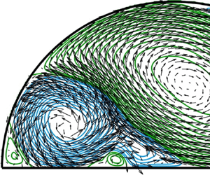
Velocity measurements and corresponding flow streamlines for  $Ro=0.2$, $S=1.6$ (experiment H in table 1) are shown in figure 4. The starting flow is shown in figure 4(a), which is qualitatively the same as that observed for $Ro=0.02$, $S=1.6$ (figure 2a). At subsequent times, however, the flow differs significantly. In this case $E^{1/2}/Ro=O(10^{-2})$, and so the time scale on which the sidewall boundary layers break down is short compared with the characteristic spin-up time scale. The data suggest the boundary layers break down after approximately one rotation period. That early boundary-layer eruption is confirmed in § 4, which leads to an eruption time of $t=7.0$. The boundary-layer breakdown results in the subsequent formation of strong cyclonic ‘secondary’ vortices in the two vertical corner regions of the tank, which grow rapidly, deforming the initial anticyclone, as shown in figure 4(b–d). As the secondary vortices grow, smaller ‘tertiary’ vortices (cyclonic and anticyclonic) form in the corner regions of the tank, as well as adjacent to the tank sidewalls, in the interstitial regions between the primary anticyclone and the secondary cyclonic cells (see figure 4d). For times $tE^{1/2}<0.5$, these much weaker tertiary vortices appear to have little effect on the bulk flow. Eventually, a dominant three-cell flow pattern emerges (figure 4e), which persists for a period, with the primary anticyclone occupying the central region of the tank, flanked either side by the two secondary cyclonic cells. During this period, the tertiary anticyclonic vortex that forms in the corner region at $(x,y)=(-1,0)$ continues to grow slowly (see figure 4e,f), until eventually a four-cell flow pattern emerges, as shown in figure 4(g). Subsequently, at $tE^{1/2}\thickapprox 2.5$, this tertiary, anticyclonic cell merges with the primary anticyclone, and a three-cell flow pattern is re-established (see figure 4h), which persists at subsequent times as the flow gradually decays due to the action of the Ekman layers at the top and bottom of each cell, and a state of solid-body rotation is approached.
Data from experiment H ( $\varOmega =1.04\ \text {rad}\ \text {s}^{-1}$, $Ro =0.2$ and $S=1.6$). Contours of the stream function estimated from the measured vorticity, superimposed on corresponding measurements of the velocity vectors $(U,V)$ (only every sixth vector is shown, to avoid saturation). The dimensionless times $t$ (and $tE^{1/2}$) at which the data were taken are (a) 3 (0.02), (b) 17 (0.1), (c) 26 (0.15), (d) 43 (0.25), (e) 87 (0.5), (f) 173 (1.0), (g) 347 (2.0), (h) 520 (3.0). The green contours (anticyclonic flow) are uniformly distributed from 0 at increments of 0.003; the blue contours (cyclonic flow) are negative and uniformly distributed from $-0.005$ at increments of $-0.005$. A scale for the velocity vectors is shown in (a).

The flow features shown in figure 4 are representative of what we observed for  $Ro=0.2$, for all values of $S$ considered. Therefore, to better understand how the flow depends on $S$, we again used measurements of the flow speed along $x=0$ at $y=0.2$ and $0.8$ to analyse the flow's rate of decay. These two points throughout remain located in the bulk structure of the primary anticyclone, which as figure 4 illustrates, is the most persistent flow feature. Hence, the measurements of flow speed at these points, which are plotted in figure 3(b) against scaled time $tE^{1/2}$, provide a reliable measure of the state of spin-up of the primary anticyclone, but are also indicative of the rate at which the bulk fluid approaches the state of solid rotation. Figure 3(b) shows that, for times $tE^{1/2}<0.5$ – this is the period in which the cyclonic corner-vortices form and the initial three-cell flow pattern emerges (see figure 4a–e) – the decay of the flow speed appears to be largely independent of $S$, except for the case $S=10$, where the rate of decay is notably slower. For times $tE^{1/2}>0.5$, the data exhibit exponential decay which appears to be consistent with the spin-up mechanism provided by the Ekman layers at the top and bottom of anticyclonic cell.
2.5. Observations for $Ro=1$ (nonlinear, spin-up from rest)

For completeness, figure 5 shows data obtained for  $Ro=1$ with $S=0$ (experiment K in table 1). In this case, $E^{1/2}/Ro=O(10^{-3})$. Comparing these data with figure 4 shows that the observed flow for $Ro=1$ is qualitatively identical to that described in § 2.4 for $Ro=0.2$; although for $Ro=1$ the flow features clearly evolve more rapidly, with secondary cyclonic corner cells that are comparatively larger, which results in greater deformation of the primary anticyclone. It is also worth noting that figure 5(g) shows the merging of the primary anticyclone with the tertiary anticyclonic cell that forms in the corner at $(x,y)=(-1,0)$ (see figure 5f); this merging event results in the subsequent emergence of the final three-cell flow pattern (shown in figure 5h), which persists at subsequent times as the flow gradually decays. (Recall, the same merging event was also observed for $Ro=0.2$.)
Data from experiment K ( $\varOmega =0.4\ \text {rad}\ \text {s}^{-1}$, $Ro =1$ and $S=0$). Contours of the stream function estimated from the measured vorticity, superimposed on corresponding measurements of the velocity vectors $(U,V)$ (only every sixth vector is shown, to avoid saturation). The dimensionless times $t$ (and $tE^{1/2}$) at which the data were taken are (a) 3 (0.03), (b) 5.4 (0.05), (c) 7.5 (0.07), (d) 9.7 (0.09), (e) 17 (0.16), (f) 32 (0.3), (g) 43 (0.4), (h) 65 (0.6). The green contours (anticyclonic flow) are uniformly distributed from 0 at increments of 0.003; the blue contours (cyclonic flow) are negative and uniformly distributed from $-0.005$ at increments of $-0.005$. A scale for the velocity vectors is shown in (a).

The experiments reported in van Heijst (Reference van Heijst1989) were likewise for  $Ro=1$ and $S=0$, although he used $\varOmega = 0.756\ \text {rad}\ \text {s}^{-1}$ (recall, we used $\varOmega = 0.4\ \text {rad}\ \text {s}^{-1}$) and a semicircular tank that was open, so the fluid's surface was free. The data in figure 5 are mostly consistent with van Heijst's observations although some key differences are notable. That is, the cyclonic corner vortices reported in van Heijst (Reference van Heijst1989) were observed to grow to an extent sufficient to fully pinch the primary anticyclone, after which the cyclonic cells were observed to merge. A likely contributing factor to this merging event is the concave parabolic free surface present in van Heijst's experiments, causing the cyclonic secondary vortices to drift inwards – an effect also reported by, for example, Carnavale, Kloosterziel & van Heijst (Reference Carnavale, Kloosterziel and van Heijst1991), van Heijst et al. (Reference van Heijst, Davies and Davis1990) and van de Konijnenberg & van Heijst (Reference van de Konijnenberg and van Heijst1997). (We thank a referee for bringing this to our attention.) Because of our flat upper boundary, we see no such effect.
At subsequent times a new anticyclonic cell was observed to form in the corner region at  $(x,y)=(-1,0)$, which led to the emergence of a final two-cell flow pattern.
3. Theoretical development of the (linear) core flow
In this section, we develop the equations and their numerical solution for the spin-up of the core. The analysis is linear, which requires only that  $Ro\ll 1$, so the presented solutions would still be marginally relevant for the $Ro=0.2$ case discussed above, were it not for the fact already noted that the vertical-wall boundary layers erupt very early in the spin-up process for $Ro=0.2$ – thereby driving the interior flow to a very different state than that predicted by the analysis below.
We take the fluid to occupy the semi-circular region  ${\mathcal {D}}=\{(r,\theta,z): 0< r<1, 0 <\theta < {\rm \pi}, 0 < z < h\}$, so $y=0$ lies along $\theta =0, {\rm \pi}$. In terms of notation, we write $\partial {\mathcal {D}}_v$ for the vertical walls and $\partial {\mathcal {D}}_h$ for the horizontal walls. It is convenient to use cylindrical polar coordinates, and so the Navier–Stokes equations are
 \begin{gather} (ru)_r + v_\theta + rw_z = 0, \end{gather}
 \begin{gather}u_t - 2v + Ro [({\bf u}\cdot \nabla)u - v^{2}/r] + p_r = E(\nabla^2 u - u/r^2 - 2v_\theta/r^2), \end{gather}
 \begin{gather}v_t + 2u + Ro [({\bf u}\cdot\nabla)v + uv/r] + p_\theta/r = E(\nabla^2 v - v/r^2 + 2u_\theta/r^2), \end{gather}
 \begin{gather}w_t + Ro({\bf u}\cdot\nabla)w + p_z ={-}\rho + E\nabla^{2} w, \end{gather}
 \begin{gather}\rho_t-Sw=0, \end{gather}
where  $(u,v,w)$ denote the velocity components in the $(r,\theta,z)$ directions. The pressure $p$ and density $\rho$ are perturbations on the background rotating, stratified state. As is usual for salt in water, we ignore the (small) diffusivity.
There are a variety of time scales in this motion: the order-one times of the Ekman-layer development and inertial, internal gravity waves; the long-time, final viscous decay for  $t=O(E^{-1})$, leading to a new steady state; and the ‘spin-up time’, $t=O(E^{-1/2})$, during which much (for moderate $S$) or not so much (for large $S$) spin-up occurs. In this section, we focus on the motion on the spin-up time scale. However, before examining the spin-up-time motion, we briefly give the result valid at very short times – before the Ekman layers begin to induce vertical motion.
3.1. Short-time behaviour
As in all impulsively started motions, the velocity vector field is irrotational, so a stream function may be used since at these early stages, the motion is purely horizontal. The vorticity equation is then easily seen to be (Foster & Munro Reference Foster and Munro2012)
 \begin{equation} \nabla_1^{2}p ={-}4, \end{equation}
where the ‘ $-4$’ is the vorticity of the pre-spin-up rigid rotation, as viewed in the frame of reference of the spun-up container, and $\nabla _1^{2}$ is the horizontal Laplacian. Thus,
 \begin{equation} u={-}p_\theta/2r,\quad v=p_r/2. \end{equation}
 The no-penetration condition is applied on  $\partial {\mathcal {D}}_v$, and then the solution is easily found, by standard separation-of-variable methods, namely,
 \begin{equation} p={-}\frac{8}{\rm \pi}\sum_{n=1}^{\infty} \frac{1-({-}1)^{n}}{(4-n^{2})n}(r^{2}-r^{n})\sin(n\theta). \end{equation}
Note that because the vertical velocity is smaller than order  $E^{1/2}$ on this time scale, the result is independent of $S$. The short-time velocity profile, $v(r,{\rm \pi} /2)$, evaluated using (3.3b) and (3.4), is plotted in figure 6 and compared with experimental data for $Ro=0.02$, obtained at time $t=3.0$.
The solid grey line shows the velocity component  $v=p_r/2$, evaluated using (3.3b) and (3.4) along $\theta ={\rm \pi} /2$, and compared with experimental data for $Ro=0.02$, obtained at time $t=3.0$. The data shown are for $S=0$ (black), $S=0.4$ (green), $S=1.6$ (blue), $S=3.0$ (red), $S=10$ (cyan). We have included estimates of uncertainty for $S=0$ (black) only, which are representative.

3.2. Flow development on the spin-up time scale
Using (3.1b) and (3.1c), the equation for the vertical vorticity component,  $\zeta$, in the absence of viscous and inertial forces is
 \begin{equation} \zeta_t-2w_z=0. \end{equation}
Combination of (3.1d) and (3.1e) gives
 \begin{equation} w={-}p_{zt}/S. \end{equation}
Then, combining (3.5) and (3.6) gives
 \begin{equation} \frac{\partial}{\partial t}[\zeta + (2/S) p_{zz}]=0. \end{equation}
If we use the reference frame of the end state, then the initial vorticity is actually  $-2$, as noted above, so
 \begin{equation} \zeta + \frac{2}{S}p_{zz} ={-}2. \end{equation}
If  $t\gg 1$, then (3.3a,b) remains valid to first order, and so the vorticity is $\zeta =\nabla _1^{2}p/2,$ and hence
 \begin{equation} \nabla_1^{2}p+\frac{4}{S}p_{zz}={-}4, \end{equation}
the generalization of (3.2) for the cases when  $p$ is dependent on $z$.
$z$.
Ekman pumping occurs on  $\partial {\mathcal {D}}_h$, and since $w=\mp E^{1/2}\zeta /2$ on $z=0,h$, (3.3a,b) and (3.6) lead to
 \begin{gather} p_{z t} ={-}\frac{S}{4}E^{1/2}\nabla_1^{2}p+{\mathcal{E}}_0\ {\rm on}\ z=0, \end{gather}
 \begin{gather}p_{z t} = \frac{S}{4}E^{1/2}\nabla_1^{2}p+{\mathcal{E}}_h\ {\rm on} z=h. \end{gather}
The symbol  ${\mathcal {E}}$ represents, as in Foster & Munro (Reference Foster and Munro2012), singular Ekman-layer eruptions at the intersections of $\partial {\mathcal {D}}_h$ and $\partial {\mathcal {D}}_v$ – a feature that we have found to be ubiquitous to non-axisymmetric, unsteady, rotating, stratified flows. That arises because no net inflow can occur into either horizontal boundary. Therefore, the quantity ${\mathcal {E}}$ must be such that
 \begin{equation} \int_0^{\rm \pi}\int_0^{1} p_{z t}\,r\,{\rm d}r\,{\rm d}\theta = 0 \ {\rm on}\ {\mathcal{D}}_h. \end{equation}
It is more convenient to use (3.9) to write (3.10a) and (3.10b) as
 \begin{gather} p_{z t} = E^{1/2}(S+p_{zz})+{\mathcal{E}}_0\ {\rm on}\ z=0, \end{gather}
 \begin{gather}p_{z t} ={-}E^{1/2}(S+p_{zz})+{\mathcal{E}}_h\ {\rm on}\ z=h. \end{gather}
For this inviscid motion, there is a no-penetration condition,
 \begin{equation} p=0\ {\rm on}\ \partial{\mathcal{D}}_v. \end{equation}
The proper form for the solution to this initial, boundary-value problem is less than obvious, because it must take account of condition (3.11). As in both Foster & Munro (Reference Foster and Munro2012) and Munro et al. (Reference Munro, Hewitt and Foster2015), the proper ansatz turns out to be
 \begin{equation} p=K_1(r,\theta,\tau) + K_2(\tau)\left(z-\frac{h}{2}\right)^{2}+P(r,\theta,z,\tau), \end{equation}
where we have introduced the spin-up time scale,
 \begin{equation} \tau=E^{1/2} t. \end{equation}
Substitution into (3.9) gives, first,
 \begin{equation} \nabla_1^{2}K_1={-}\frac{8}{S}K_2, \end{equation}
and the  $K_1$ solution may be written as the Fourier–Bessel series
 \begin{equation} K_1=\frac{8K_2}{S} \sum_{m=1}^{\infty} \sum_{n=1}^{\infty} \frac{c_{mn}b_n}{\alpha_{mn}^{2}}J_n(\alpha_{mn}r)\sin(n\theta), \end{equation}
where  $\alpha _{mn}$ is the $m^{\rm th}$ zero of $J_n(z)$.
Here,  $P$ is written also as a double Fourier series,
 \begin{equation} P=\sum_{m=1}^{\infty} \sum_{n=1}^{\infty} F_{mn}(z,\tau)J_n(\alpha_{mn}r)\sin(n\theta), \end{equation}
and its substitution into (3.9) leads to
 \begin{equation} \sum_{m=1}^{\infty}\sum_{n=1}^{\infty}(F''_{mn,\tau}-\mu_{mn}^{2}F_{mn}) J_n(\alpha_{mn}r)\sin(n\theta)={-}S. \end{equation}
Here the prime denotes a  $z$ derivative, and the subscript $\tau$ is for a $\tau$ derivative.
We here define the following:
 \begin{gather} a_{mn} = \int_0^{1}rJ_n(\alpha_{mn}r)\,{\rm d}r, \end{gather}
 \begin{gather}b_n = \frac{2}{n{\rm \pi}}[1-({-}1)^{n}], \end{gather}
 \begin{gather}c_{mn}=\frac{a_{mn}}{{\displaystyle\int_0^{1}} r J_n^{2}(\alpha_{mn}r)\,{\rm d}r}=\frac{2a_{mn}}{[J_{n-1}(\alpha_{mn})]^{2}}. \end{gather}
The orthogonality of the radial and azimuthal eigenfunctions applied to (3.19) produces the differential equation for  $\{F_{mn}\}$,
 \begin{equation} F''_{mn}-\mu_{mn}^{2}F_{mn}={-}Sc_{mn}b_n,\quad \mu_{mn}\equiv\sqrt{S}\,\alpha_{mn}/2, \end{equation}
whose solution with appropriate symmetry is
 \begin{equation} F_{mn}=\frac{Sc_{mn}b_n}{\mu_{mn}^{2}}+d_{mn}(\tau)\cosh[\mu_{mn}(z-h/2)]. \end{equation}
Note that the leading term in this expression is the impulsive start motion, so therefore  $d_{mn}(0)=0$. (Insertion of that quantity into (3.14) and (3.18) can be shown to give a result equivalent to (3.4).)
What remains are two items. First, we satisfy boundary condition (3.12a),
 \begin{align} &\sum_{m=1}^{\infty}\sum_{n=1}^{\infty} F'_{mn,\tau}(0,\tau)J_n(\alpha_{mn}r)\sin(n\theta)-K_{2,\tau}h \nonumber\\ &\quad = S+\sum_{m=1}^{\infty} \sum_{n=1}^{\infty} F''_{mn}(0,\tau)J_n(\alpha_{mn}r)\sin(n\theta)+2K_2+{\mathcal{E}}_0\ {\rm on}\ z=0. \end{align}
The condition on  $z=h$ is also satisfied by the choice of the hyperbolic cosine in (3.22). The second condition is that the area integral of the left-hand side of this equation must be zero. Therefore, substitution into (3.11) gives
 \begin{equation} hK_{2,\tau}=\sum_{m=1}^{\infty} \sum_{n=1}^{\infty} F'_{mn,\tau}(0,\tau)a_{mn}b_n. \end{equation}
Inserting solution (3.22), and integrating once in time gives
 \begin{equation} hK_2={-}\sum_{m=1}^{\infty} \sum_{n=1}^{\infty} d_{mn}(\tau) a_{mn}\mu_{mn}b_n\sinh(\mu_{mn}h/2). \end{equation}
Using orthogonality in (3.23) leads to the boundary condition
 \begin{equation} F'_{mn,\tau}(0,\tau)-F_{mn}^{\prime\prime}(0, \tau) = (S+hK_{2,\tau}+2K_2)c_{mn}b_n. \end{equation}
Substitution of (3.22) then leads to the evolution equation for  $\{d_{mn}\}$,
 \begin{equation} d_{mn,\tau}+\mu_{mn}T_{mn}^{{-}1}d_{mn}={-}\frac{S+hK_{2,\tau}+2K_2}{\mu_{mn}S_{mn}} c_{mn}b_n, \end{equation}
where
 \begin{equation} S_{mn}\equiv \sinh(\mu_{mn}h/2),\quad C_{mn}\equiv\cosh(\mu_{mn}h/2),\quad T_{mn}\equiv \tanh(\mu_{mn}h/2). \end{equation}
In the Appendix A, we give the solution that arises by setting time derivatives in these equations to zero. The ‘steady state’ is of course the long-time solution on the spin-up time scale. In § 3.3, below, we report the numerical solution to the equation set (3.27).
3.3. Numerical, unsteady solution
Numerical solution of (3.27) may be found by standard methods. We use an implicit scheme for each  $d_{mn}$, with $d_{mn}(0)=0$ as noted above. At each instant of time, the summation for $K_2$ is then performed, using (3.25).
It should be noted that, because of the eigenfunction decomposition of the solution, there is a wide range of eigenvalues for the differential equation system –  $\tanh (\mu _{mn}h/2)/\mu _{mn}$ – so the system exhibits stiffness and care must be taken to choose very small time steps. Typically, time steps of order $10^{-5}$ have proven to be adequate when truncating the Fourier–Bessel series at $50$ terms. We have found that the transient response over the ranges of $S$ studied is very rapid – coming to a steady value by $\tau \approx 0.3$ – except for $S\equiv 0$, which is a bit slower, but more of that later. So, the long, slow decay of values of $v$ on the midline $\theta ={\rm \pi} /2$ seen in figure 3 is not due to this transient process but is, as we shall see, the result of the viscous boundary layers growing into the interior.
Figure 7(a) shows computed values of the velocity component  $v$ across the tank on $\theta ={\rm \pi} /2$ for several values of $S$, at spin-up time $\tau =E^{1/2}t=1.0$. Note that spin-up is close to being achieved at this time for $S=0$ and nearly so for $S=0.4$, whereas for $S=3.0$, for example, little has changed from the initial, impulsive-start profile – shown by the grey, dashed line. Clearly these profiles do not correspond to the results discussed in § 2.3 because of the presence of boundary layers on the vertical walls. To further clarify that matter, the time evolution of the velocity component $v$, at $r=0.2$ on $\theta ={\rm \pi} /2$, is shown in figure 7(b) for each value of $S$. The plots stand in contrast with what is shown in figure 3. The reason for that is that the time scale for inviscid decay of the core flow is $E^{-1/2}$, and as we shall see in § 4, the vertical-wall boundary layers develop on a scale $Ro^{-1}$. For the case $R=0.02$, the ratio of these two scales is 0.25 to 0.39 in the experiments reported here (see table 1), and both effects occur simultaneously – hence the differences in the two figures.
(a) Core flow velocity profile along  $\theta ={\rm \pi} /2$, at $tE^{1/2}=1.0$ for $S=0$ (black), $S=0.4$ (green), $S=1.6$ (blue), $S=3.0$ (red). The grey, dashed line is the $S$-independent profile for the initial, impulsive start. Results for $S=10$ have not been included here because they are barely distinguishable from $S=3.0$. (b) Time evolution of $v$ at $r=0.2$, $\theta ={\rm \pi} /2$ for $S=0$ (black), $S=0.4$ (green), $S=1.6$ (blue), $S=3.0$ (red).

3.3.1. A limiting case: $S\rightarrow 0$

The time evolution of the flow for the non-stratified case may be found by analytical means alone; we let  $S\rightarrow 0$ in the analysis of the previous section. Expanding the solution as a perturbation series in $S$,
$S$,
 \begin{equation} p = p_0 + Sp_1 + \cdots, \end{equation}
substitution into (3.9) gives
 \begin{equation} p_{0,zz} = 0 \Rightarrow p_0 = A(r,\theta,t), \end{equation}
where the evident even symmetry has been invoked. Then, to next order,
 \begin{equation} p_{1,zz} ={-}1-\frac{1}{4}\nabla_1^{2}A. \end{equation}
Again, using even symmetry,
 \begin{equation} p_1={-}\frac{1}{2}(z-h/2)^{2}\left[1+\frac{1}{4}\nabla_1^{2}A\right]. \end{equation}
Substituting into the lower-wall boundary condition, (3.12), leads to the equation for the vorticity,
 \begin{equation} \left[\frac{\partial}{\partial t}+\frac{2E^{1/2}}{h}\right]\nabla_1^{2}A=0, \end{equation}
whose solution is
 \begin{equation} \nabla_1^{2} A=(\nabla_1^{2} A)_{t=0}e^{{-}2E^{1/2}t/h}={-}4e^{{-}2E^{1/2}t/h}. \end{equation}
So, for  $S=0$, the flow is the initial, impulsive-start motion, multiplied by the Ekman decay. For consistency with the foregoing, we may write the result as
 \begin{equation} p_0 = 4\sum_{m=1}^{\infty} \sum_{n=1}^{\infty} \frac{c_{mn}b_n}{\alpha_{mn}^{2}}J_n(\alpha_{mn}r)\sin(n \theta)\,e^{{-}2E^{1/2}t/h}. \end{equation}
(The double series here that multiplies the temporal exponential can easily be shown to be mathematically equivalent to (3.4).) Notice that the  $S=0.4$ result in figure 7 shows a rapid change near the boundary, not in evidence in this solution. The reason for that is that $S\rightarrow 0$ is a singular limit: for $S$ small but not identically zero, there is a thin layer of width $S^{1/2}$ near both $y=0+$ and $r=1-$, clearly evident in computations for small $S$. The unsteady development of the flow within this $S^{1/2}$ layer is very complicated indeed, and not given here for the sake of brevity. In Appendix A, however, we do include the steady solution for this zone.
The  $S\rightarrow 0$ limit is fascinating in an additional way. From the analysis in § 3, one can show that the damping coefficients for the eigenmodes are distinct and have absolute values that are larger than $2E^{1/2}/h$. (See Foster & Munro (Reference Foster and Munro2012) and Munro et al. (Reference Munro, Hewitt and Foster2015) for a description of a ‘normal mode’ approach to solutions of (3.27).) All are needed to describe the motion. However, as $S\rightarrow 0$, this complicated spectral structure becomes degenerate: all of the damping coefficients coalesce into the single value $2E^{1/2}/h$, evident in (3.34).
4. Sidewall boundary layers
The layers on  $\partial {\mathcal {D}}_v$ begin growing as Rayleigh layers, but continue to grow and develop as nonlinear boundary layers, as we shall see. As noted in Foster & Munro (Reference Foster and Munro2012), so long as $E =o(S^{4/3})$, the boundary layer is a conventional Prandtl boundary layer on the horizontal velocity components, but for $S$ values that are extremely small, the boundary layer is a nonlinear Stewartson ‘quarter layer’. In either case, the layer is essentially two-dimensional. Only for $E$ of the order $S^{4/3}$ is there a three-dimensional structure to the layer. Considering here the boundary layer on $y=0$, the unscaled sidewall boundary layer equation is
 \begin{equation} U_t+2{\mathcal{R}} E^{1/2} (U-U_e)+Ro(UU_x+VU_y)-U_{e t}-Ro U_eU_{ex}=E U_{yy}, \end{equation}
where  $U_e$ is obtained from the numerical results discussed in § 3.3. The quantity ${\mathcal {R}}$ multiplies the vortex-stretching term, ${\mathcal {R}}=1$ for the $S=0$ case reported in this paper, and is zero for all $S\ne 0$ cases reported here. In both situations, the layer is essentially two-dimensional, with $z$ dependence arising only parametrically through $U_e$.
We may deduce important time scale information from the equation itself. First, for very short times, the Rayleigh layer has width  $\sqrt {E t}$, but it develops into the nonlinear boundary layer whose width scales with $\sqrt {E/Ro}$, since the corresponding time scale is $Ro^{-1}$. Hence, $\tau \sim E^{1/2}/Ro$ is the characteristic time for nonlinear boundary-layer evolution. For experiments C and H (figures 2 and 4 show streamline data for these cases), that ratio is $0.25$ and $0.025$ (see table 1) for $Ro=0.02$ and $Ro=0.2$, respectively – suggestive of the order of magnitude for $\tau$ at boundary-layer breakdown.
For purposes of the standard, boundary-layer computation whose results are discussed below,  $y$ is scaled by $E^{1/4}$ and time scale $\tau$ is used. Figure 8(a) shows boundary-layer displacement thickness on the straight wall for $Ro=0.02$ and $S=1.6$, at different times. The data in figure 8(a) at time $\tau =0.05$ (blue curve) shows the boundary layer is attached to the wall, which is in agreement with the streamline data shown in figure 2(a) (which are also for $Ro=0.02$, $S=1.6$), at the slightly earlier time $\tau =0.02$. Figure 2(b), for $\tau =0.5$, shows evidence of a weak cyclonic cell in the corner region at $(x,y)=(-1,0)$, apparently still confined to the boundary layer; with an instantaneous stagnation point that has formed a distance of approximately $0.3$ from the corner, consistent with the eruption location shown by the green curve in figure 8(a), at $\tau =0.29$. Just beyond $\tau =0.5$, the boundary-layer computation fails, and clearly by the time $\tau =1$ shown in figure 2(c), the boundary layer is well separated with a well-defined corner cell.
Boundary-layer displacement thickness,  $\delta ^{+}$, scaled with $E^{1/4}$, versus distance $x$ along the straight wall, for $S=1.6$. (a) $Ro=0.02$. The times $\tau =E^{1/2}t$ for which results are shown are $0.05$ (blue), $0.10$ (black), $0.20$ (red), $0.29$ (green). (b) $Ro=0.2$. The times $\tau$ for which results are shown are $0.01$ (blue), $0.02$ (black), $0.03$ (red), $0.044$ (green).

In the case shown in figure 8(b), for  $Ro=0.2$ and $S=1.6$, the larger Rossby number not surprisingly means an earlier-time boundary-layer eruption – as expected based on the simple scaling arguments above. The calculation fails in fact at $\tau =0.0443$ for this case. Comparing figure 8(b) with experimental data in figure 4(b) (also for $Ro=0.2$ and $S=1.6$), both confirm the boundary-layer attachment at $\tau =0.02$. Clearly in figure 4(b), for $\tau =0.1$, the boundary layer has already erupted into the interior, consistent with the theoretical eruption time determined above.
Similar computations and discussion may be detailed for the boundary layer on the curved wall, but are not presented here since there is not much more to be learned from them – except to observe that the eddy forming along that wall seems to be more elongated and modifies the central core flow somewhat less.
It is interesting to compare the boundary-layer behaviour for  $S=0$. Figure 9(a) shows the displacement thickness for different times. We note that the boundary layer develops an internal eddy, seen in figure 9(b). However, the layer actually stops growing and becomes thinner as noted by the blue curve, for $\tau =4$, when the velocities are now very small. Comparing the green curve in figure 9(a) with figure 8(a), it appears that the layer is about to erupt, but that never happens. That is because $U_e$ in (4.1) is going to zero exponentially, as indicated in (3.35), so the nonlinear term in (4.1) scales with
 \begin{equation} \frac{Ro}{E^{1/2}}\, {\rm e}^{{-}2\tau/h}, \end{equation}
and hence the boundary layer at longer times (with  ${\mathcal {R}}=1$ as noted earlier) is a steady, linear Stewartson layer. It appears in this case that the eddy is wholly contained within the boundary layer, which is consistent with the instantaneous streamline image shown in figure 9(b), for $\tau =1.0$. Since for $S=0$, the edge velocity is going to zero exponentially, but the boundary layer is tending toward breakdown. These two competing effects mean that there is a critical Rossby number below which the boundary layer does not have a finite-time eruption. Computations show that that critical Rossby number is $0.022$.
Results for  $S=0$ and $Ro=0.02$. (a) Boundary-layer displacement thickness, $\delta ^{+}$, scaled with $E^{1/4}$, versus distance $x$ along the straight wall. The times $\tau =E^{1/2}t$ for which the data are shown are $0.1$ (black), $0.50$ (red), $1.0$ (green), $4.0$ (blue). (b) Instantaneous streamline pattern in the boundary layer in the vicinity of $(x,y)=(-1,0)$, at $\tau =1.0$.

4.1. Composite solutions
In order to compare with the experimental data presented in § 2, we need to combine the inviscid core solutions of § 3 with the boundary-layer calculations of § 4. The difficulty is that, over most of the time range for the flow speeds plotted in figure 3 (i.e.  $0\leqslant \tau \leqslant 4$), the boundary layers on both straight and curved walls have erupted near the corners (see figure 8), which ultimately led to the formation of cyclonic corner cells. Since the boundary layers are more-or-less intact at $x=0$, we will assume for the sake of the theory/experiment comparisons that the corner cells are isolated and do not much alter the central primary anticyclone. It is clear from the data and discussions presented in § 2 that this assumption is not valid for $Ro=0.2$ and 1, and so here comparisons are made only for the case $R=0.02$. Under that assumption, we can numerically generate a composite solution to patch together both boundary layers to the core flow to yield velocity profiles across the container, to compare with the experiments. Figure 10 shows such composite solutions at times $\tau =E^{1/2}t=0.5$ and $1.0$ (grey lines), compared with corresponding data from the experiments. To within experimental uncertainty, there is good agreement for $S=0$ and 0.4. For $S=1.6$ the correspondence is good for $0.2\leqslant r\leqslant 0.8$, at both times; however, in the regions close to the sidewalls the measured flow speed is significantly less than the composite solution. For $S=3.0$, the correspondence is less good.
Composite solutions for the velocity component  $v$ on $\theta ={\rm \pi} /2$ (thick grey lines) compared with corresponding experimental data, for times $\tau =E^{1/2}t=0.5$ (left-hand plots) and $1.0$ (right-hand plots). The data are for (a,b) $S=0$, (c,d) $S=0.4$, (e,f) $S=1.6$, (g,h) $S=3.0$.

5. Final remarks
We have presented details of the way in which a rotating, stratified fluid in a semi-circular tank adjusts to a slightly higher rotation rate, as measured by the Rossby number,  $Ro$. The flow evolution is dominated by Ekman-pumping effects in the core, and by the formation and subsequent breakdown of the vertical-wall boundary layers. The two characteristic time scales associated with these processes are $t\sim E^{-1/2}$ and $t\sim Ro^{-1}$, respectively. Here we have reported experiments for $E^{1/2}=O(10^{-2})$, $Ro=0.02$, 0.2 and 1, with the Burger number ( $S$) varied between 0 and 10. When the spin-up and boundary-layer breakdown times are comparable ( $E^{1/2}/Ro\sim 10^{-1}$), the observed flow is dominated by the gradual spin-up of the initial anticyclone, with the cyclonic vorticity generated in the sidewall boundary layers remaining confined to the immediate neighbourhood of the sidewall and corner regions. The presence of a background density gradient acts to inhibit vertical motion and Ekman pumping, and so the rate of spin-up is dependent on the strength of the fluid's stratification. In this regime we found that for $S=0$ the fluid is fully spun up after $tE^{1/2}\thickapprox 2$. However, after the same period for $S\gtrsim 1$, the regions of peak flow speed within the anticyclone had decayed to approximately 50 % of their initial value.
A markedly different flow was observed for  $E^{1/2}/Ro\sim 10^{-2}$ and $10^{-3}$, dominated by the formation of strong, cyclonic secondary vortices in the fluid near the four vertical corners of the tank, which grow rapidly and deform the initial anticyclone. Eventually, a three-cell flow pattern emerges, with the initial anticyclone occupying the tank's centre, flanked on either side by a cyclonic cell. This flow pattern persists and fluid is gradually spun up. Again, for $S=0$ the fluid is fully spun up after $tE^{1/2}\thickapprox 2$. However, after the same period for $S\gtrsim 1$, the peak flow speed within the anticyclone had decayed to approximately 30 % of the initial value, suggesting the effects associated with stratification are somewhat reduced in this regime.
For both ranges of  $E^{1/2}/Ro$, we have found that computed boundary-layer eruption times agree well with what is observed in those experiments. For $E^{1/2}/Ro\sim 10^{-1}$, the velocity profiles on the vertical midplane determined by forming a composite solution of core flow and boundary layers agree well with experiment, particularly if $S$ is not too large, because in this $Ro$ range, the corner vortices remain more-or-less confined to those corners where they first form.
Finally, there are several results in this study that stand in contrast to what has been reported for the square cylinder, in Munro et al. (Reference Munro, Hewitt and Foster2015) and Foster & Munro (Reference Foster and Munro2012). First, we were intrigued by the work reported in van Heijst (Reference van Heijst1989) for the semi-circular geometry, and wondered if, in the stratified case, we would see qualitatively different flow evolution from what we found in the square cylinder, since, while asymmetric, the square does have two planes of symmetry rather than the single plane for the semicircle. The answer to that question seems to be that the boundary-layer eruptions exert a much stronger effect on the core flow than for the square cylinder. In fact, with the corner vortices more-or-less confined to the four corners in the square cylinder case, the large core eddy is very nearly axisymmetric; from a rather näive point of view, these vortices effectively round the corners. Nothing like that happens here. That point is certainly related to a second observation, namely, that the theoretical/experimental comparisons are, at least from visual inspection, much better for the square cylinder than for the semicircle. Third, we have computed here the time evolution of the core flow, instead of determining the frequencies and mode shapes associated with the motion. The importance of that is that the actual computed nonlinear boundary-layer velocity profiles are used to construct the ‘composite velocity profiles’, rather than using the simpler Rayleigh-layer model of Foster & Munro (Reference Foster and Munro2012). Finally, we have now seen what was not so evident in the square cylinder: the decay of the interior velocities is dominated by the growth of the sidewall boundary layers, and not by the Ekman-layer-induced decay of the linear, core flow. However, since the temporal growth of the  $S=0$ wall layer is much less than for $S\ne 0$, the spin-up in that case is dominated by the ‘inviscid’ core-velocity decay.
Declaration of interests
The authors report no conflict of interest.
Appendix A. Steady-state core flow
A.1. Steady-state solution
Putting the time derivatives to zero in (3.27) leads to the equation
 \begin{equation} \tilde d_{mn}={-}\frac{S+2\tilde K_2}{\mu_{mn}^{2}C_{mn}} c_{mn}b_n. \end{equation}
The tilde denotes this steady solution. Multiplying this equation by  $a_{mn}\mu _{mn}b_n S_{mn}$, and summing over all $m$ and $n$, then using (3.25), leads to
 \begin{equation} -h\tilde K_2={-}(S+2\tilde K_2) \sum_{m=1}^{\infty} \sum_{n=1}^{\infty} \frac{a_{mn}c_{mn}b_n^{2}}{\mu_{mn}} T_{mn}. \end{equation}
Solving,
 \begin{equation} \tilde K_2=\frac{S\sigma}{2(h-\sigma)},\quad \sigma \equiv 2\sum_{m=1}^{\infty} \sum_{n=1}^{\infty} \frac{a_{mn}c_{mn}b_n^{2}}{\mu_{mn}} T_{mn}. \end{equation}
Hence, from (A1),
 \begin{equation} \tilde d_{mn}={-}\frac{Sh}{h-\sigma}\frac{c_{mn}b_n}{\mu_{mn}^{2}C_{mn}}. \end{equation}
Putting the pieces together, we have, for this steady state, that
 \begin{align} p&=\frac{4~h}{h-\sigma}\sum_{m=1}^{\infty} \sum_{n=1}^{\infty} \frac{c_{mn}b_n}{\alpha_{mn}^{2}}\left\{1-\frac{\cosh[\mu_{mn}(z-h/2)]}{C_{mn}}\right\} J_n(\alpha_{mn}r)\sin(n\theta)\nonumber\\ &\quad +\frac{S\sigma}{2(h-\sigma)}\left(z-\frac{h}{2}\right)^{2}. \end{align}
For purposes of comparison, the very short-time response is given in (3.4), and may be shown to be equivalent to
 \begin{equation} p_{\textit{short}}=4\sum_{m=1}^{\infty} \sum_{n=1}^{\infty} \frac{c_{mn}b_n}{\alpha_{mn}^{2}}J_n(\alpha_{mn}r)\sin(n\theta). \end{equation}
There are several observations to be made from (A5) and (A6) about the end of processes on this time scale. The last term in (A5), of course, merely alters the isopycnals, and is not dynamically relevant.
A.2. Comments on the steady state
We summarize below principal observations on the steady flow.
(i) From (A5), since the square bracket inside the sum is zero at both
$z=0$ and $z=h$, the fluid is fully spun up near the upper and lower boundaries for all $S$.(ii) If
$S=O(1)$, then virtually all of the core is not spun up on this time scale.(iii) For
$S=o(1)$, $\sigma =O(1)$. Careful examination of the sum indicates that $p=O(S)$ in the core, so there is a weak interior flow in this steady state, and the core is essentially spun up fully on this time scale.(iv) For
$S\gg 1$,
(A7)The number\begin{equation} \sigma = \frac{4}{S^{1/2}}\sum_{m=1}^{\infty} \sum_{n=1}^{\infty} \frac{a_{mn}c_{mn}b_n^{2}}{\alpha_{mn}}=\frac{4 \times 0.793}{S^{1/2}}. \end{equation}$0.793$ is determined by computing the double summation. Since $S$ is large, the hyperbolic functions take simple forms, and so (A5) becomes
(A8)(The last term has been dropped as noted before.) In this expression,\begin{align} p &= \frac{4~h}{h-0.793/S^{1/2}}\sum_{m=1}^{\infty} \sum_{n=1}^{\infty} \frac{c_{mn}b_n}{\alpha_{mn}^{2}}\left[1-\exp\left(-\frac{1}{2}S^{1/2}\alpha_{mn} Z\right)\right] \nonumber\\ &\quad \times J_n(\alpha_{mn}r)\sin(n\theta). \end{align}$Z=z$ in $z< h/2$ and $Z=h-z$ in $z>h/2$. So, we see that the core is still at the short-time behaviour, and the regions within $S^{-1/2}$ of each horizontal boundary are partially spun up. In fact, we see that – as we found previously in Foster & Munro (Reference Foster and Munro2012) – there is ‘over-spin’, since
(A9)in the core.\begin{equation} p \sim \left[1+\frac{3.17}{hS^{1/2}}\right]p_{short}+\text{exponentially small terms}, \end{equation}(v) Examining the initial problem (3.2), (3.12a), it is evident that both
$S\rightarrow 0$ and $S\rightarrow \infty$ are singular limits. As noted in item (iv) above, in the case of large $S$, that is seen in the layers of width $S^{-1/2}$ near top and bottom walls – immediately apparent from (A8). However, the nature of the eigenfunction expansion (A5) masks the small-$S$ structure. We noted in item (iii) the core is fully spun up for small $S$ on this time scale, but figure 7 shows a complication – in fact, there is a layer on $\partial {\mathcal {D}}_v$ in which the fluid is not fully spun up. The non-uniformity can be inferred from (A5): The hyperbolic cosine inside the square bracket is near one when its argument is very small, leading to the conclusion, (iii). However, if $\alpha _{mn}$ is sufficiently large, then the argument of the hyperbolic cosine is not small even if $S$ is small. In fact, the argument is order one when $\alpha _{mn}^{-1}$, a characteristic radial length scale, is order $S^{1/2}$. Thus, we expect a wall layer of width $S^{1/2}$ at small $S$ values. The structural details may be shown more clearly by a small-$S$ asymptotic analysis of § 3.3.1 and (3.12a), but that is not included here for brevity.(vi) As promised in § 3.3.1, the solution for the pressure in the
$S^{1/2}$ zone inside $r=1$ is given by
(A10)where\begin{equation} p=S\sum_{n=1}^{\infty} r_n \sin(n{\rm \pi} z/h)\exp\left[-\frac{2n{\rm \pi}(1-r)}{S^{1/2}h}\right], \end{equation}(A11)so the speed – order\begin{equation} r_n ={-}\frac{4 h^{2}}{n^{3}{\rm \pi}^{3}}[1-({-}1)^{n}]-\frac{h^{2}}{n{\rm \pi}}[1+({-}1)^{n}], \end{equation}$S$ in the interior, as noted above – scales with $S^{1/2}$ in this narrow region.


We have seen here that this ‘steady state’ is not really achieved as described at finite Rossby number, since the growing boundary layers on the straight wall and the half-circle erode the ‘steady’ values in the above solutions near  $\partial {\mathcal {D}}_v$.


 Open access