2.1. Derivation of the modified Orr–Sommerfeld equations with FSI extension term

To first understand the basic instability mechanisms occurring during the interaction of fluid and flexible leaflet tissue, we derive an approach incorporating FSI into the classic Orr–Sommerfeld equations. We conduct temporal LSA for multiple base flows (figure 1) in a simplified one-dimensional model with and without a flexible wall representing the valve leaflet.

Figure 1.

Streamwise velocity field in the aortic root with inserted BHV. Base flow profiles are extracted along the green line (aortic jet) with boundary conditions representing a rigid wall (blue) and flexible wall (red) for the ($b_1$) wall-bounded case, ($b_2$) pure shear flow case and ($b_3$) FSI case with flexible wall.

We study three different configurations. Configuration $b_1$ represents the aortic jet bounded by two fixed leaflets at $\tilde {y}=\pm 0.5$. Configuration $b_2$ features the same aortic jet after leaving the valve orifice. Two rigid walls represent the aortic walls at $\tilde {y}=\pm 1$ and we assume zero flow between the aortic jet and the rigid walls. In configuration $b_3$ the aortic jet is bounded by flexible leaflets at $\tilde {y}=\pm 0.5$ which separate the jet from the zero-flow region between the flexible leaflets and the rigid aortic walls at $\tilde {y}=\pm 1$. The definition of the base flow profile for the aortic jet is described in Appendix A. As the applied base flows are slightly asymmetric, we cannot exploit symmetry to retrieve strictly sinous or varicose modes, but need to consider the full domain.

The derivation of the eigenvalue problem starts with the non-dimensional incompressible Navier–Stokes equations (non-dimensional quantities indicated with a tilde) including a force density $\tilde {\boldsymbol {f}}_{{FSI}}$ which we introduce to account for the interaction between fluid and flexible wall:

(2.1)$$\begin{gather} \frac{\partial \tilde{\boldsymbol{u}}_{f}}{\partial t} + \rho_{f} (\tilde{\boldsymbol{u}}_{f} \boldsymbol{\cdot} \boldsymbol{\nabla}) \tilde{\boldsymbol{u}}_{f} ={-}\boldsymbol{\nabla} \widetilde{p_{f}} + \frac{1}{\textit{Re}} \nabla^2 \tilde{\boldsymbol{u}}_{f} + \tilde{\boldsymbol{f}}_{{FSI}}, \nonumber\\ \boldsymbol{\nabla} \boldsymbol{\cdot} \tilde{\boldsymbol{u}}_{f} = 0 . \end{gather}$$

The non-dimensionalized force density $\tilde {\boldsymbol {f}}_{{FSI}}$ depends on a material-specific constant $\xi$ (derivation described in Appendix B) and the second derivative of the wall displacements $\tilde {\eta }_{-}$ at $\tilde {y}=\tilde {y}_{-}=-0.5$ and $\tilde {\eta }_{+}$ at $\tilde {y}=\tilde {y}_{+}=0.5$ to model the effect of wall tension. It is given as

(2.2)\begin{equation} \tilde{\boldsymbol{f}}_{{FSI}} = \left(0, \delta(\tilde{y}-\tilde{y}_{-}) \xi \frac{\partial^2 \tilde{\eta}_-}{\partial \tilde{x}^2} + \delta(\tilde{y}-\tilde{y}_{+}) \xi \frac{\partial^2 \tilde{\eta}_+}{\partial \tilde{x}^2} \right). \end{equation}

This formulation with the Dirac delta function $\delta (\kern0.7pt y)$ follows the immersed boundary concept by Peskin (Reference Peskin2002). A similar problem with a main focus on flexural stiffness of the structure has been studied by Lebbal, Alizard & Pier (Reference Lebbal, Alizard and Pier2022). Here, flexural stiffness (associated with the fourth derivative of the wall displacement) is neglected because of the thin membrane-like geometry of the leaflet.

A normal mode ansatz for the perturbation velocity components $[u^{\prime },v^{\prime } ]$ and perturbation displacements $[\eta ^{\prime }_-,\eta ^{\prime }_+]$ is applied to the linearized extended Navier–Stokes equations:

(2.3)\begin{equation} [u^{\prime}, v^{\prime}, \eta^{\prime}_-, \eta^{\prime}_+ ] = [\hat{u}(\tilde{y}), \hat{v}(\tilde{y}), \hat{\eta}_-, \hat{\eta}_+ ]\exp [\mathrm{i} \alpha (\tilde{x} - c\tilde{t})], \end{equation}

with associated amplitudes $[\hat {u}(\tilde {y}), \hat {v}(\tilde {y}), \hat {\eta }_-, \hat {\eta }_+ ]$, wavenumber $\alpha$ and complex phase speed $c = \omega /\alpha$.

The displacement amplitudes $[\hat {\eta }_-,\hat {\eta }_+]$ are substituted by the vertical velocity amplitude $\hat {v}$ considering interface conditions at $\tilde {y}=[\tilde {y}_{-},\tilde {y}_{+}]$:

(2.4)$$\begin{gather} \hat{v} |_{\tilde{y}=\tilde{y}_{-}} ={-}\mathrm{i} \alpha c \hat{\eta}_{-} , \end{gather}$$

(2.5)$$\begin{gather}\hat{v} |_{\tilde{y}=\tilde{y}_{+}} ={-}\mathrm{i} \alpha c \hat{\eta}_{+} . \end{gather}$$

The insertion of the base flow profile $U = u(x_1,y_1,t ) / U_{max}$ leads to a modified Orr–Sommerfeld equation with FSI extension terms:

(2.6) \begin{align} & \left[(U-c)(\mathcal{D}^2-\alpha^2)c-U^{\prime\prime}c+\frac{\mathrm{i}}{\alpha{\textit{Re}}} (\mathcal{D}^2-\alpha^2)^2 c\right.\nonumber\\ &\left.\quad \vphantom{\frac{\mathrm{i}}{\alpha{\textit{Re}}}} -\alpha^2\delta(\tilde{y}-\tilde{y}_{-})\xi-\alpha^2 \delta(\tilde{y}-\tilde{y}_{+})\xi \right] \hat{v} = 0, \end{align}

with $\mathcal {D} = {\rm d} / {\rm d}\tilde {y}$ and the Reynolds number defined as

(2.7)\begin{equation} {\textit{Re}} = \frac{U_{max} L \rho_{f}}{\mu_{f}}, \end{equation}

with $L$ as the spanwise orifice of fully open, stable valve leaflets. In this linearized form the positions $y_\pm$ are fixed at ${\pm }0.5$.

The resulting quadratic eigenvalue problem

(2.8)\begin{equation} (c^2 \boldsymbol{\mathsf{A}} + c \boldsymbol{\mathsf{B}} + \boldsymbol{\mathsf{C}}) \hat{v} = 0 \end{equation}

is transformed into a generalized eigenvalue problem (Tisseur Reference Tisseur2000)

(2.9)\begin{equation} \begin{pmatrix} -\boldsymbol{\mathsf{B}} & -\boldsymbol{\mathsf{C}} \\ \boldsymbol{\mathsf{I}} & \boldsymbol{\mathsf{0}} \end{pmatrix}\varphi = c \begin{pmatrix} \boldsymbol{\mathsf{A}} & \boldsymbol{\mathsf{0}} \\ \boldsymbol{\mathsf{0}} & \boldsymbol{\mathsf{I}}, \end{pmatrix}\varphi \end{equation}

with $\varphi = (c \hat {v},\hat {v})^{\rm T}$ and the boundary conditions $\hat {v}={\partial \hat {v}}/{\partial \tilde {y}} = 0$ at $\tilde {y}=\pm 1$.

2.2. Temporal LSA

First, base flow $b_1$ with a flow profile between two rigid walls is analysed. It reflects the inflow condition of the aortic jet between two fixed leaflets before entering the AAo. The flow remains linearly stable up to ${\textit {Re}}=5240$.

Beforehand, we define a wavenumber region considered relevant in our later investigation of a finite valve leaflet. Taking into account its one-sided fixation and the finite leaflet length $H$, we define wavelengths $\lambda _{min} = H$ and $\lambda _{max} = 4 H$ as $\alpha _0=5.55$ and $\alpha _{1/4}=1.39$, respectively. As indicated by the schematic drawings in figure 2 and 5 the interval $[\lambda _{min},\lambda _{max}]$ defines a range of typical wavelengths observed in fluttering valve leaflets (compare, for example, with figure 6 in Becsek et al. (Reference Becsek, Pietrasanta and Obrist2020)).

Figure 2.

Growth rate $\omega _i$ as a function of wavenumber $\alpha$ for ${\textit {Re}} = 3318$ for base flow $b_2$ (blue) and base flow $b_3$ (green). Eigenfunctions and velocity fields are later given for wavenumbers $\boldsymbol {I}$ and $\boldsymbol {II}$ in figures 3 and 4.

The analysis is conducted for base flows $b_2$ and $b_3$ to quantify the effect of the flexible wall on stability regions. Growth rates $\omega _i = \mbox {Im}(c \alpha )$ for a physiologically relevant Reynolds number of $Re=3318$ (see Appendix A) are shown in figure 2. The separation of zero-flow and jet-flow regions by a flexible wall decreases the range of unstable wavenumbers to $\alpha _3=[0,12.7]$ for $b_3$ compared with the pure shear flow case $b_2$ which is unstable in $\alpha _2=[0,19.7]$. Evaluating the corresponding range of unstable physical wavelengths $\lambda$, base flow $b_2$ shows a minimum unstable wavelength of $\lambda _2=0.28H$ while base flow $b_3$ becomes unstable for a minimum wavelength of $\lambda _3 = 0.44 H$. Also, the maximum growth rate of $b_3$ is smaller and located at a lower wavenumber ($\omega _{i,3,max} = 1.32$ at $\alpha _{3}=6.0$ corresponding to $\lambda _{3} = 0.93 H$) compared with pure shear flow $b_2$ ($\omega _{i,2,max} = 1.62$ at $\alpha _{2}=8.2$ corresponding to $\lambda _{2}= 0.68 H$).

Figure 3 for $\alpha _0$ and figure 4 for $\alpha _{1/4}$ give further insight into the unstable mode pairs at ${\textit {Re}}=3318$ of base flows $b_2$ and $b_3$. Real and imaginary parts of the normalized eigenfunction $\bar {v}$ are shown together with the corresponding reconstructed two-dimensional streamwise velocity fields $\tilde {u}$. The two-dimensional velocity field is reconstructed by

(2.10)$$\begin{gather} \tilde{u}(\tilde{x},\tilde{y}) = U(\tilde{y}) + \epsilon \mbox{Re}(\bar{u}(\tilde{y}) \exp [\mathrm{i} \alpha \tilde{x}]) , \end{gather}$$

(2.11)$$\begin{gather}\tilde{v}(\tilde{x},\tilde{y}) = \epsilon \mbox{Re}(\bar{v}(\tilde{y}) \exp [\mathrm{i} \alpha \tilde{x}]) , \end{gather}$$

with $\bar {u} = \mathrm {i} \mathcal {D} \bar {v} / \alpha$ based on the continuity equation. The wall displacement $[\tilde {\eta }_{-}(\tilde {x}),\tilde {\eta }_{+}(\tilde {x})]$ is reconstructed by applying the previously defined interface conditions (2.5):

(2.12)$$\begin{gather} \tilde{\eta}_{-}(\tilde{x}) = \epsilon \mbox{Re}\left(\frac{\mathrm{i}}{c\alpha} \bar{v}|_{\tilde{y}_{-}} \exp [\mathrm{i} \alpha \tilde{x}]\right) , \end{gather}$$

(2.13)$$\begin{gather}\tilde{\eta}_{+}(\tilde{x}) = \epsilon \mbox{Re}\left(\frac{\mathrm{i}}{c\alpha} \bar{v}|_{\tilde{y}_{+}} \exp [\mathrm{i} \alpha \tilde{x}]\right). \end{gather}$$

Figure 3.

Normalized amplitude $\tilde {v}$ and dimensionless streamwise velocity field $\tilde {u}$ for $\epsilon = 0.08$ with streamlines of (a) the most unstable mode of base flow $b_2$, (b) the second most unstable mode of base flow $b_2$, (c) the most unstable mode of base flow $b_3$ and (d) the second most unstable mode of base flow $b_3$ for wavenumber $\alpha _{0}$ at ${\textit {Re}}=3318$ (corresponding to $\boldsymbol {II}$ in figure 2).

Figure 4.

Normalized amplitude $\bar {v}$ and dimensionless streamwise velocity field $\tilde {u}$ for $\epsilon = 0.08$ with streamlines of (a) the most unstable mode of base flow $b_2$, (b) the second most unstable mode of base flow $b_2$, (c) the most unstable mode of base flow $b_3$ and (d) the second most unstable mode of base flow $b_3$ for wavenumber $\alpha _{1/4}$ at ${\textit {Re}}=3318$ (corresponding to $\boldsymbol {I}$ in figure 2).

For $\alpha _0$ in figure 3, two unstable modes exist for each base flow of which one affects the upper and the other the bottom shear layer ($b_2$) or flexible wall ($b_3$). While the real part of the eigenfunction peaks at the distinct vertical location of maximum shear ($b_2$) or flexible wall ($b_3$), the location of the imaginary maximum of smaller amplitude is shifted slightly towards the jet core. Considering the reconstructed two-dimensional flow fields, base flow $b_2$ shows classical Kelvin–Helmholtz (KH) flow features within the shear layer. The addition of the flexible wall for base flow $b_3$ leads to similar flow patterns in the wall region at either $\tilde {y}_{-}$ or $\tilde {y}_{+}$. For smaller wavenumbers such as $\alpha _{1/4}$ in figure 4, we can observe an interaction between both shear layers ($b_2$) or flexible walls ($b_3$). While higher wavenumbers show a one-sided eigenfunction destabilizing the flow at only one of the vertical locations $\tilde {y}_{-}$ or $\tilde {y}_{+}$, lower wavenumbers are associated with eigenfunctions which couple the modes of both shear layers ($b_2$) or flexible walls ($b_3$).

When evaluating the neutral stability curves in figure 5, the critical Reynolds number for KH modes corresponding to configuration $b_2$ is higher (${\textit {Re}}_{KH} = 299$) than for FSI modes corresponding to configuration $b_3$ (${\textit {Re}}_{FSI} = 184$). An overlapping region of both KH and FSI modes exists for a large Reynolds number and wavenumber range which includes physiologically relevant Reynolds numbers and wavenumbers. Therefore, both instabilities (KH and FSI) are suspected to be present simultaneously after valve opening.

Figure 5.

Neutral stability curves for pure shear flow (base flow $b_2$, indicated in blue) and FSI case (base flow $b_3$, indicated in green).

Figure 6 shows the dependency of the eigenvalues on wavenumber $\alpha$ for base flows $b_2$ and $b_3$. The growth rate $\omega _i = \mbox {Im}(c \alpha )$ of the unstable eigenmode pair is displayed against the phase speed $c_r = \omega _r/\alpha$ at ${\textit {Re}}=3318$. In general, the phase speed $c_r$ decreases with increasing wavenumber for both base flow configurations. Growth rates $\omega _i$ of KH modes (base flow $b_2$) peak at higher wavenumber compared with FSI-related modes (base flow $b_3$). The FSI-related modes generally grow slower than KH modes; however, phase speeds are higher. For ${\textit {Re}}=3318$, the most unstable KH mode has a phase speed $c_r = \omega _r / \alpha$ of $c_{r,2}(\alpha _2) = 0.424$ while the most unstable FSI-related mode is faster with a phase speed of $c_{r,3}(\alpha _3) = 0.649$. In conclusion, unstable KH modes seem to grow faster than unstable FSI-related modes for their unstable wavenumber range. Also, we observe less dependency of the phase speed of the KH modes on the wavenumber. In comparison, FSI-related modes depend stronger on the wavenumber. While small wavelengths travel slowly, the phase speed of higher wavelengths is higher and varies more related to the wavenumber.

Figure 6.

Path of locus for the unstable eigenmode pairs of base flow $b_2$ (pure shear flow, blue) and base flow $b_3$ (flexible wall, green) for wavenumbers $\alpha$ at Reynolds number ${\textit {Re}}=3318$.

3.1. Governing equations and numerical method

After the investigation of instability mechanisms in a simplified one-dimensional model, we now increase the modelling complexity by conducting highly-resolved two-dimensional FSI simulations of a parametrized aortic geometry. Hereby, we aim to obtain a deeper insight into more complex flow features as well as their temporal and spatial evolution.

The interaction of valve and blood flow is implemented within an in-house high-fidelity FSI solver developed for applications including blood flow and soft tissue on hybrid high-performance computing platforms. The flow field is solved by a GPU-accelerated high-order Navier–Stokes solver based on Henniger, Obrist & Kleiser (Reference Henniger, Obrist and Kleiser2010) and Zolfaghari & Obrist (Reference Zolfaghari and Obrist2021) on a structured, staggered grid using the incompressible Navier–Stokes equations:

(3.1)\begin{equation} \left.\begin{gathered} \rho_{f} \frac{\partial \boldsymbol{u}_{f}}{\partial t} + \rho_{f} (\boldsymbol{u}_{f} \boldsymbol{\cdot} \boldsymbol{\nabla}) \boldsymbol{u}_{f} ={-}\boldsymbol{\nabla} p_{f} +\mu_{f} \Delta \boldsymbol{u}_{f} + \boldsymbol{f} ,\\ \boldsymbol{\nabla} \boldsymbol{\cdot} \boldsymbol{u}_{f} = 0, \end{gathered}\right\} \end{equation}

with the fluid density $\rho _{f}$, dynamic viscosity $\mu _{f}$, pressure $p_f$, time $t$ and, in the present case, two-dimensional fluid velocity field $\boldsymbol {u}_{f} = [u_{f,x},u_{f,y}]$. The added force term $\boldsymbol {f}$ accounts for FSI.

Temporal discretization is realized by a third-order Runge–Kutta time stepping while the fluid is spatially discretized by a sixth-order finite difference scheme.

An unstructured grid is used for the discretization of the structural domain, which is solved by a finite element solver using the full elastodynamic equations:

(3.2)\begin{equation} \rho_{s} \frac{\partial^2 \boldsymbol{u}_{s}}{\partial t^2} - \boldsymbol{\nabla}\boldsymbol{\cdot} \boldsymbol{\mathsf{P}} = 0, \end{equation}

with the structural density $\rho _{s}$, the displacement field $\boldsymbol {u}_{s}$ and the Piola–Kirchhoff stress tensor $\boldsymbol{\mathsf{P}}$.

The interaction of fluid and structure motion is realized by a modified immersed boundary method based on variational transfer with the following interface conditions:

(3.3)\begin{equation} \left.\begin{gathered} \boldsymbol{u}_{f} = \frac{\partial \boldsymbol{u}_{s}}{\partial t} ,\\ J^{{-}1} \boldsymbol{\mathsf{P}} \boldsymbol{\mathsf{F}}^{\rm T} \boldsymbol{n} = {{{\boldsymbol{\sigma}}}}_{f} \boldsymbol{n}, \end{gathered}\right\} \end{equation}

including the Cauchy stress $\boldsymbol{\sigma} _{f}$ and the deformation gradient $\boldsymbol{\mathsf{F}} = \boldsymbol {\nabla } \boldsymbol {u}_{s} + \boldsymbol{\mathsf{I}}$ with its associated determinant $J = \textrm {det} \boldsymbol{\mathsf{F}}$.

Details of the FSI solver as well as its experimental and numerical validation can be found in Nestola et al. (Reference Nestola, Becsek, Zolfaghari, Zulian, De Marinis, Krause and Obrist2019) and Becsek et al. (Reference Becsek, Pietrasanta and Obrist2020).

The two-dimensional, rectangular fluid domain is resolved with a structured grid of $2209 \times 897$ points on a domain of an extent of $11.18r_{A} \times 4.55r_{A}$ with $r_A$ as the annular radius in order to resolve the onset of hydrodynamic instabilities. Grid stretching was applied which reduces the minimal mesh width to around $35\,\mathrm {\mu }$m in the immediate vicinity of the valve. The unstructured solid grid consists of approximately $11\,300$ triangular elements.

With a time step size of $1\,\mathrm {\mu }$s, the computational time for the simulation of the systolic acceleration (200 ms) amounts to around 1500 node hours on $8$ nodes of a Cray XC40/XC50 high-performance computer.

3.2. Two-dimensional parametrized aortic model

The problem set-up in figure 7(a) is a model of an aortic root with an inserted bioprosthetic valve. The actual threefold symmetry of the three-dimensional aortic root with three sinus bulbs and corresponding valve leaflets is simplified to a two-dimensional problem by considering a mirrored longitudinal cut through the middle plane of a leaflet. Generally, the structural domain is divided into aortic wall, valve stent and valve leaflet and separated in the fluid regions as annulus ($\delta \varOmega _{A}$), sinus ($\delta \varOmega _{S}$) and AAo ($\delta \varOmega _{AAo}$). The aortic wall geometry is based on data of Haj-Ali et al. (Reference Haj-Ali, Marom, Ben Zekry, Rosenfeld and Raanani2012) and Reul et al. (Reference Reul, Vahlbruch, Giersiepen, Schmitz-Rode, Hirtz and Effert1990) and the curvature of the valve leaflets on the bioprosthetic aortic valve Edwards Intuity Elite 21 (Edwards Lifesciences, Irvine, CA, USA). Geometrical parameters are listed in table 1 which are constant throughout each analysed case.

Figure 7.

(a) Parametrized two-dimensional model of the aortic wall with inserted bioprosthetic valve. Constant parameters (black) are referenced in table 1 and variable parameters (red) in table 2. (b) Systolic acceleration defined as the inflow flow rate from the left ventricular outflow tract.

Table 1.

Constant parameters of the parametrized aortic model relative to the annular radius $r_A$.

We additionally introduce the parameters sinus height ($h_{STJ}$) and AAo radius ($r_{AAo}$) in order to evaluate the influence of aortic wall geometry on instabilities in the aortic root. Parametrization values (table 2) were chosen according to realistic anatomical ranges extracted from various studies on aortic root morphology by Bahlmann et al. (Reference Bahlmann, Nienaber, Cramariuc, Gohlke-Baerwolf, Ray, Devereux, Wachtell, Kuck, Davidsen and Gerdts2011), Buellesfeld et al. (Reference Buellesfeld2013), Mirea et al. (Reference Mirea, Maffessanti, Gripari, Tamborini, Muratori, Fusini, Claudia, Fiorentini, Plesea and Pepi2013), Vriz et al. (Reference Vriz2014) and Boraita et al. (Reference Boraita, Heras, Morales, Marina-Breysse, Canda, Rabadan, Barriopedro, Varela, De La Rosa and Tuñón2016). As a result, we define three cases: initial configuration (indicated as case A), increased sinus height (indicated as case B) and decreased AAo radius (indicated as case C).

Table 2.

Variable parameters of the parametrized aortic model relative to the annular radius $r_A$ with the parameters sinus height $h_{STJ}$ and AAo radius $r_{AAo}$. Evaluated configurations are indicated as initial configuration (A), increased sinus height (B) and decreased AAo radius (C).

The opening phase of bioprosthetic aortic valves is completed after a duration of around 20 ms. Thereafter, the valve remains in the open position before the asynchronous closing starts at a third of the full cardiac cycle corresponding to a physical time of about 0.3 s (Vennemann et al. Reference Vennemann, Rösgen, Heinisch and Obrist2018). As we aim to investigate hydrodynamic instabilities initiating laminar–turbulent transition leading to turbulent flow during early systole as shown in Becsek et al. (Reference Becsek, Pietrasanta and Obrist2020), we limit our study to the systolic acceleration phase of a duration of about 0.2 s as defined in figure 7(b).

Inflow conditions are enforced by the fringe region technique described in Nordström, Nordin & Henningson (Reference Nordström, Nordin and Henningson1999) for a periodic fluid domain. A penalization term $\boldsymbol {f}_{{fringe}} (\boldsymbol {x})$ is added to the right-hand side of the Navier–Stokes equations within a fringe region located at the left ventricular outflow tract as described in Becsek et al. (Reference Becsek, Pietrasanta and Obrist2020). A physiological inflow profile at a defined cardiac output is ensured by tuning of the fringe function. By suppressing lateral velocity components within the fringe region, entering fluctuations due to the periodic fluid domain are damped. Here, we impose a pressure difference of 8 mmHg across the fringe region corresponding to the average systolic transvalvular pressure gradient.

The fluid is modelled as incompressible and Newtonian with material properties similar to those of blood ($\mu _{f}=0.004$ Pa s, $\rho _{f}=1050$ kg m$^{-3}$). The aortic wall and the valve stent are assumed to be rigid while we apply a hyperelastic, nonlinear neo-Hookean material model with a shear modulus of $\mu _{s}=5.0\times 10^{5}$ Pa to the flexible valve leaflets. The shear modulus was tuned in order to match leaflet oscillation amplitudes extracted from a less resolved three-dimensional case of a bioprosthetic valve with leaflets modelled by a fibre-reinforced Holzapfel–Gasser–Ogden model (Holzapfel, Gasser & Ogden Reference Holzapfel, Gasser and Ogden2000). Figure 8 shows the temporal evolution of the leaflet tip displacement for four shear moduli previously applied in studies of Hiromi Spühler & Hoffman (Reference Hiromi Spühler and Hoffman2020) ($\mu _{s}=3.3\times 10^{4}$ Pa), Chandra et al. (Reference Chandra, Rajamannan and Sucosky2012) ($\mu _{s}=1.2\times 10^{5}$ Pa), Bavo et al. (Reference Bavo, Rocatello, Iannaccone, Degroote, Vierendeels and Segers2016) ($\mu _{s}=3.4\times 10^{5}$ Pa) and De Hart et al. (Reference De Hart, Peters, Schreurs and Baaijens2000) ($\mu _{s}=5.0\times 10^{5}$ Pa) in comparison with the three-dimensional simulation.

Figure 8.

Temporal evolution of leaflet tip displacements perpendicular to the longitudinal aortic axis for four shear moduli according to two-dimensional studies for a neo-Hookean model of (a) Hiromi Spühler & Hoffman (Reference Hiromi Spühler and Hoffman2020), (b) Chandra, Rajamannan & Sucosky (Reference Chandra, Rajamannan and Sucosky2012), (c) Bavo et al. (Reference Bavo, Rocatello, Iannaccone, Degroote, Vierendeels and Segers2016) and (d) De Hart et al. (Reference De Hart, Peters, Schreurs and Baaijens2000) in comparison with a less resolved three-dimensional reference study using a Holzapfel–Gasser–Ogden (HGO) model.

3.3. Numerical results

3.3.1. The influence of FSI: rigid versus flexible leaflet

To assess the effect of FSI on laminar–turbulent transition, we compare the base configuration starting with closed leaflets (case A) from figure 7 with a rigid leaflet case fixed in open position (indicated as AR). The rigid leaflet shape of case AR is extracted from the flexible case A immediately after full valve opening. In particular, we pick the deformed leaflet shape prior to the onset of (a) leaflet motion and (b) non-zero transversal velocities within the shear layer created in the wake of the leaflet (hereafter referred to as ‘leaflet shear layer’).

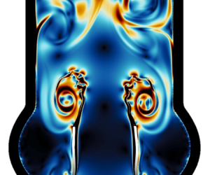
Figure 9 shows the instantaneous viscous shear stress magnitude $|{{{\tau }}}|$ at five time instances for the rigid leaflet case AR (top row) and the flexible leaflet case A (bottom row). Three main flow phenomena seem to occur sequentially for both rigid and flexible cases:

1. (i) Starting vortex (figure 9a). Early during systolic acceleration, a distinct starting vortex is formed which is advected downstream.

2. (ii) Vortex–wall interaction (figure 9b–d). The starting vortex is advected and elongates in the streamwise direction. Due to the transversal confinement by the aortic wall and the associated no-slip boundary condition at the wall, a secondary vortex is created upstream of the starting vortex. This smaller vortex rebounds from the aortic wall and moves towards the leaflet shear layer. The ejection of a secondary vortex when a sufficiently strong primary vortex (here the starting vortex) impinges at a wall is well documented (Walker et al. Reference Walker, Smith, Cerra and Doligalski1987; Orlandi & Verzicco Reference Orlandi and Verzicco1993).

3. (iii) Shear layer instability (figure 9e). When the secondary vortex reaches the outer side of the shear layer, we observe growing shear layer instabilities.

Figure 9.

Instantaneous viscous shear stress magnitude $| {{{\tau }}} |$ for (AR) rigid leaflet case and (A) flexible leaflet case for aortic wall configuration A at (a) $t=0.10$ s, (b) $t=0.1175$ s, (c) $t=0.135$ s, (d) $t=0.1525$ s and (e) $t=0.17$ s. Secondary vortical structures forming after the impingement of the starting (primary) vortex on the aortic wall are shown by the red arrows.

Both cases show growing vortical structures within the shear layer at a similar time which suggests that the general mechanisms do not seem to be influenced by the open or closed starting position of the rigid or flexible leaflet, respectively. Moreover, the occurrence of shear layer instabilities seems to be independent of mechanisms related to FSI. This is further supported by the observation that the flexible leaflets of case A remain stable during the initial onset of vortical structures reminiscent of KH-like vortex roll-up within the shear layer. This is in agreement with the LSA predicting KH modes for this flow regime.

The impact of FSI on the downstream flow field starts to become relevant during the growth phase of the shear layer instability. Figure 10 shows instantaneous shear stress magnitudes for the flexible leaflet case at time instances after those displayed in figure 9. As predicted by LSA, we observe an FSI-related instability of the flexible leaflets. While figure 10(a) shows the onset of leaflet motion, we observe a stronger influence of leaflet motion on the downstream flow field by vortex shedding from the leaflet tips in figure 10(b). This is consistent with the repeated formation of vortex rings at the valve orifice associated with oscillatory leaflet motion shown for the three-dimensional model by Becsek et al. (Reference Becsek, Pietrasanta and Obrist2020). Eventually, figure 10(c) possibly indicates another instability leading to small-scale vortices within the larger vortex downstream of the leaflets.

Figure 10.

Instantaneous viscous shear stress magnitude $|{{{\tau }}} |$ for aortic wall configuration A at (a) $t=0.1875$ s, (b) $t=0.1945$ s and (c) $t=0.2$ s.

3.3.2. Effect of aortic root geometry

To assess the influence of morphological features on instability mechanisms, we simulate the cases A (base configuration), B (increased sinus height) and C (decreased AAo radius) as defined in table 2. Instantaneous viscous shear stress magnitudes at multiple time instances throughout systolic acceleration are shown in figure 11. Cases A and B display similar temporal and spatial evolution of the starting vortex. In contrast, case C exhibits an early elongation of the starting vortex caused by the earlier vortex–wall interaction due to the narrower AAo. As described before, confinement of the downstream flow region causes the formation of a second smaller vortex approaching the leaflet shear layer (red arrows in figure 11) which is followed by instability in the leaflet shear layers. In case C, this shear layer instability appears earlier than in cases A and B (see figure 11b). Likewise, the second shear-related instability leading to smaller shear-layer vortices (green arrows) occurs also earlier for case C than for cases A and B.

Figure 11.

Instantaneous viscous shear stress magnitude $|{{{\tau }}} |$ for aortic wall configurations (A) initial configuration, (B) increased sinus height and (C) decreased AAo radius at (a) $t=0.125$ s, (b) $t=0.15$ s, (c) $t=0.175$ s and (d) $t=0.20$s. Secondary vortical structures forming after the impingement of the starting (primary) vortex on the aortic wall are shown by the red arrows.

Figure 12 shows the evolution of the transversal velocity at six leaflet thicknesses, $x=6t_L$, downstream of the instantaneous leaflet position as well as the transversal leaflet tip velocity. First, we observe the initial opening of the leaflet (completed at $t\approx 0.08$ s) which is almost identical for all three aortic configurations. After the opening phase, the leaflet remains in a stable position until the onset of transversal leaflet and fluid motion. For cases A and B, this occurs at $t\approx 0.13$ s, while we observe an earlier onset of leaflet and fluid motion for case C ($t\approx 0.11$ s). After this onset, we find growing oscillations of leaflet tip and fluid at a frequency of approximately 55 Hz. These oscillations are reminiscent of leaflet fluttering observed in BHVs in experimental studies (Vennemann et al. Reference Vennemann, Rösgen, Heinisch and Obrist2018).

Figure 12.

Temporal evolution of transversal fluid velocities extracted at $x=6t_L$ downstream of the instantaneous leaflet tip position (blue) and transversal leaflet tip velocity (black) for aortic wall configurations (a) initial configuration (case A), (b) increased sinus height (case B) and (c) decreased AAo radius (case C) with the onset of transversal oscillations indicated by the red arrow.

Although the same qualitative sequence of flow phenomena shows for every aortic wall configuration, there are major differences in the timing and onset of the different mechanisms. In particular, a shorter distance between leaflet tip and aortic wall appears to lead to earlier shear layer perturbations.