
I. INTRODUCTION
Graphical models are useful tools for describing the geometric structure of networks in numerous applications such as energy, social, sensor, biological, and transportation networks [Reference Shuman, Narang, Frossard, Ortega and Vandergheynst1] that deal with high-dimensional data. Learning from these high-dimensional data requires large computation power which is not always available [Reference Koller and Friedman2,Reference Jordan3]. The hardware limitation for different applications forces us to compromise between the accuracy of the learning algorithm and its time complexity by using the best possible approximation algorithm given the constrained graph. In other words, the main concern is to compromise between model complexity and its accuracy by choosing a simpler, yet informative model. To address this concern, many approximation algorithms are proposed for model selection and imposing structure given data. For the Gaussian distribution, the covariance selection problem is presented and studied in [Reference Dempster4,Reference Lauritzen5]. This paper goes beyond the seminal work of [Reference Huang, Liu, Pourahmadi and Liu6] on model approximation by formulating the model approximation problem as a detection problem. The detection problem allows us to look at the model approximation problem in a broader and more accurate way, by being able to study new measures to assess the approximation quality and to look at the distribution of the sufficient statistic under each hypothesis. Here, we introduce the Correlation Approximation Matrix (CAM) and use the CAM to assess the quality of the approximation by relating the CAM to information divergences (e.g. Kullback–Leibler (KL) divergence) and the Area Under the Curve (AUC). The CAM, AUC, and reverse KL divergence give new qualitative insights into the quality of the model approximation.
The ultimate purpose of the covariance selection problem is to reduce the computational complexity in various applications. One of the special approximation models is the tree approximation model. Tree approximation algorithms are among the algorithms that reduce the number of computations to get quicker approximate solutions to a variety of problems. If a tree model is used, then distributed estimation algorithms such as message passing algorithm [Reference Kschischang, Frey and Loeliger7] and the belief propagation algorithm [Reference Loeliger, Dauwels, Hu, Korl, Ping and Kschischang8] can easily be applied and are guaranteed to converge to the maximum likelihood solution.
The Chow-Liu algorithm discussed in [Reference Chow and Liu9] gives a method for constructing a tree that minimizes the KL divergence between the model and model tree approximation. The Chow-Liu Minimum Spanning Tree (MST) algorithm for Gaussian distributions is to find the optimal tree structure using a KL divergence cost function [Reference Dempster4]. The Chow-Liu MST algorithm constructs a weighted graph by computing pairwise mutual information and then utilizes one of the MST algorithms such as the Kruskal algorithm [Reference Kruskal10] or the Prim algorithm [Reference Prim11]. How good is the Chow-Liu solution that minimizes the KL divergence? Can we formulate other measures to assess the model approximation? These questions are becoming more important to answer as we study engineering applications that are modeled by larger and larger graphical models thus requiring simple model approximations. Before addressing these questions (which is the topic of this paper), we discuss other work and an application.
Other research in approximating the correlation matrix and the inverse correlation matrix with a more sparse graph representation while retaining good accuracy include the first order Markov chain approximation [Reference Kruskal10], penalized likelihood methods such as LASSO [Reference Lauritzen5,Reference Meinshausen and Buhlmann12], and graphical LASSO [Reference Friedman, Hastie and Tibshirani13]. The first order Markov chain approximation method uses a regret cost function to output first- order Markov chain structured graph [Reference Khajavi and Kuh14] by utilizing a greedy type algorithm. Penalized likelihood methods use an L1-norm penalty term in order to sparsify the graph representation and eliminate some edges. Recently, a tree approximation in a linear, underdetermined model is proposed in [Reference Khajavi15] where the solution is based on expectation, maximization algorithm combined with the Chow Liu algorithm.
Sparse modeling has many applications in distributed signal processing and machine learning over graphs. One important application is monitoring the electric power grid at the distribution level. The smart grid is a promising solution that delivers reliable energy to consumers through the power grid when there are uncertainties such as distributed renewable energy generation sources. Smart grid technologies such as smart meters and communication links are added to the distribution grid in order to obtain the high-dimensional, real-time data and information and overcome uncertainties and unforeseen faults. The future grid will incorporate distributed renewable energy generation such as solar photovoltaics, with these energy sources being intermittent and highly correlated. Here we can model both energy sources and energy users by nodes on a graph with edges representing electric feeder lines. The graphs for distribution networks can be very large with renewable energy sources adding complexity to the graphs. This necessitates the need for model selection.
This paper discusses the quality of the model selection, focusing on the Gaussian case, i.e. covariance selection problem. We ask the following important question: “given an approximation model, is the model approximation of the covariance matrix for the Gaussian model a good approximation?” To answer this question, we need to pick a closeness criterion which has to be coherent and general enough to handle a wide variety of problems and also has asymptotic justification [Reference Kadane and Lazar16]. In many applications, the – KL divergence has been proposed as a closeness criterion between the original distribution and its model approximation distribution [Reference Dempster4,Reference Chow and Liu9]. Besides that, other closeness measures and divergences are used for the model selection. One example is the use of the reverse KL divergence as the closeness criterion in variational methods to learn the desired approximation structure [Reference MacKay17].
In this paper, we bring a different perspective to quantify the quality of the model approximation problem by formulating a general detection problem. This formulation gives statistical insight on how to quantify a selected model. Also, the detection problem formulation leads to the calculation of the log-likelihood ratio test (LLRT) statistic, the KL divergence and the reverse KL divergence as well as the receiver operating characteristic (ROC) curve and the area under the ROC curve (AUC) where the AUC is used as the accuracy measure for the detection problem. The detection problem formulation is a different approach which gives us a broader view by determining whether a particular model is a good approximation or not. Remark. The AUC does not depend on a specific operating point on the ROC and broadly summarizes the entire detection framework. It also effectively combines the detection probability and the false-alarm probability into one measure. The AUC determines the inherent ability of the test to distinguish (in conventional detection problem) or not to distinguish (in model approximation problem) between two hypotheses/models. More specifically, the detection formulation and particularly the AUC gives us additional insight about any approximation since it is a way to formalize the model approximation problem. This fact is the contribution of this paper and leads to qualitative insights by computing AUC and its bounds. For Gaussian data, the LLRT statistic simplifies to an indefinite quadratic form. We define a key quantity which is the CAM. The CAM is the product of the original correlation matrix and the inverse of the model approximation correlation matrix. For Gaussian data, this matrix contains all the information needed to compute the information divergences, the ROC curve and the area under the ROC curve, i.e. the AUC. We also show the relationship between the CAM, the AUC and the Jeffreys divergence [Reference Jeffreys18], the KL divergence and the reverse KL divergence. We present an analytical expression to compute the AUC for a given CAM that can be efficiently evaluated numerically. We then show the relation between the AUC, the KL divergence, the LLRT statistics, and the ROC curve. We also present analytical upper and lower bounds for the AUC which only depend on eigenvalues of the CAM. Throughout the discussion section, we pick the tree approximation model as a well-known subset of all graphical models. The tree approximation is considered since they are widely used in literature and it is much simpler performing inference and estimation on trees rather than graphs that have cycles or loops. We perform simulations over synthetic and real data for several examples to explore and discuss our results. Simulation results indicate that 1 −AUC is decreasing exponentially as the number of nodes in the graph increases which is consistent with the analytical results obtained from the AUC upper and lower bounds.
The rest of this paper is organized as follows. In Section 2, we give a general framework for the detection problem and the corresponding sufficient test statistic, the log-likelihood ratio test. The LLRT for Gaussian data as well as its distribution under both hypotheses are also presented in this section. The ROC curve and the AUC definition, as well as an analytical expression for the AUC, are given in Section 3. Section 4 provides analytical lower and upper bounds for the AUC. The lower bound for the AUC uses the Chernoff bound and is a function of the CAM eigenvalues. The upper bound is obtained by finding a parametric relationship between the AUC and the KL and reverse KL divergences. Then, Section 5 presents the tree approximation model and provides some simulations over synthetic examples as well as real solar data examples and investigates the quality of the tree approximation based on the numerically evaluated AUC and also its analytical upper and lower bounds. Finally, Section 6 summarizes results of this paper and discusses future directions for research.
II. DETECTION PROBLEM FRAMEWORK
In this section, we present a framework to quantify the quality of a model selection. More specifically, we formulate a detection problem to distinguish between the covariance matrix of a multivariate normal distribution and an approximation of the aforementioned covariance matrix based on the given model. A key quantity, the Correlation Approximation Matrix (CAM) is introduced in this section and for Gaussian data, we can calculate the KL divergence and log-likelihood ratios, that all depend on the eigenvalues of the CAM.
A) Model selection problem
We want to approximate a multivariate distribution by the product of lower order component distributions [Reference Lewis-II19]. Let random vector X ∈ ℝn, have a distribution with parameter Θ, i.e. X ~ f X(x). We want to approximate the random vector X, with another random vector associated with the desired model.Footnote 1 Let the model random vector  $\underline {{X}}_{\cal {M}} \in {\open R}^n$ have a distribution with parameter $\Theta _{\cal M}$, associated with the desired model, i.e. $\underline {{X}} \sim f_{\underline {{X}}_{\cal M}}(\underline {{x}})$. Also, let ${\cal G}=({\cal V},\, {\cal E}_{\cal M})$ be the graph representation of the model random vector $\underline {{X}}_{\cal {M}}$ where sets ${\cal V}$ and ${\cal E}_{\cal M}$ are the set of all vertices and the set of all edges of the graph representing of $\underline {{X}}_{\cal {M}}$, respectively. Moreover, ${\cal E}_{\cal M} \subseteq \psi $ where ψ is the set of all edges of a complete graph with vertex set ${\cal V}$.
Remark
Covariance selection is presented in [Reference Dempster4]. Moreover, tree model as a special case for the model selection is discussed in subsection A.
B) General detection framework
The model selection is extensively studied in the literature [Reference Dempster4]. Minimizing the KL divergence between two distributions or the maximum likelihood criterion are proposed in many state of the art works to quantify the quality of the model approximation. A different way to look at the problem of quantifying the quality of the model approximation is to formulate a detection problem [Reference Lehmann and Romano20]. Given the set of data, the goal of the detection problem is to distinguish between the null hypothesis and the alternative hypothesis. To set up a detection problem for the model selection, we need to define these two hypotheses as follows
- The null hypothesis, ${\cal H}_0$: data are generated using the known/original distribution,
- The alternative hypothesis,
${\cal H}_1$: data are generated using the model/approximated distribution.


Given the set up for the null hypothesis and the alternative hypothesis, we need to define a test statistic to quantify the detection problem. The likelihood ratio test (the Neyman–Pearson (NP) Lemma [Reference Neyman and Pearson21]) is the most powerful test statistic where we first define the LLRT as
 $$l(\underline{{x}}) = {\log} \displaystyle{f_{\underline{{X}}}(\underline{{x}}|{\cal H}_1)\over f_{\underline{{X}}}(\underline{{x}}|{\cal H}_0)} = {\log} \displaystyle{f_{\underline{{X}}_{\cal M}}(\underline{{x}})\over f_{\underline{{X}}}(\underline{{x}})}$$
where  $f_{\underline {{X}}}(\underline {{x}}|{\cal H}_0)$ is the random vector X distribution under the null hypothesis while $f_{\underline {{X}}}(\underline {{x}}|{\cal H}_1)$ is the random vector X distribution under the alternative hypothesis.
Let l(X) be the LLRT statistic random variable. Then, we define the false-alarm probability and the detection probability by comparing the LLRT statistic under each hypothesis with a given threshold, τ, and computing the following probabilities
- The false-alarm probability, P 0(τ), under the null hypothesis,
${\cal H}_0$: $P_{0}({\brtau}) = \hbox{Pr} ( l(\underline {{X}}) \geq {\brtau} | {\cal H}_0)$,- The detection probability, P 1(τ), under the alternative hypothesis,
${\cal H}_1$: $P_{1}({\brtau}) = \hbox{Pr} ( l(\underline {{X}}) \geq {\brtau} | {\cal H}_1)$.


The NP Lemma [Reference Neyman and Pearson21] is the most powerful test at a given false-alarm rate (significant level). The most powerful test is defined by setting the false-alarm rate  $P_0 ({\brtau}) = \bar {P_0}$ and then computing the threshold value τ = τ0 such that $\Pr (l(\underline {{X}}) \geq {\brtau}_0 | {\cal H}_0 ) = \bar {P_0}$.
Definition 1
The KL divergence between two multivariate continuous distributions with probability density functions (PDF) pX(x) and qX(x) is defined as
 $${\cal D} ( p_{\underline{{X}}}(\underline{{x}})||q_{\underline{{X}}}(\underline{{x}}) ) = \displaystyle\int_{{\cal X}} p_{\underline{{X}}}(\underline{{x}}) \log \displaystyle{p_{\underline{{X}}}(\underline{{x}}) \over q_{\underline{{X}}}(\underline{{x}})} \; d \underline{{x}}$$
where  ${\cal X}$ is the feasible set.
Throughout this paper, we may use other notation such as the KL divergence between two covariance matrices for zero-mean Gaussian distribution case or the KL divergence between two random variables in order to present the KL divergence between two distributions.
Proposition 1
Expectation of the LLRT statistic under each hypothesis is
-
${\rm E} \left (l(\underline {{X}}) | {\cal H}_0 \right ) = - {\cal D}( f_{\underline {{X}}}(\underline {{x}}) || f_{\underline {{X}}_{\cal M}}(\underline {{x}}))$,-
${\rm E} \left (l(\underline {{X}}) | {\cal H}_1 \right ) = {\cal D}( f_{\underline {{X}}_{\cal M}}(\underline {{x}}) || f_{\underline {{X}}}(\underline {{x}}))$.


Proof: Proof is based on the KL divergence definition. □
Remark
The relationship between the NP lemma and the KL divergence is previously stated in [Reference Eguchi and Copas22] with the similar straightforward calculation, where the LLRT statistic loses power when the wrong distribution is used instead of the true distribution for one of these hypotheses.
In a regular detection problem framework, the NP decision rule is to accept the hypothesis  ${\cal H}_1$ if the LLRT statistic, l(x), exceeds a critical value, and reject it otherwise. Furthermore, the critical value is set based on the rejection probability of the hypothesis ${\cal H}_0$, i.e. false-alarm probability. However, we pursue a different goal in the approximation problem scenario. Our goal is to approximate a model distribution with PDF $f_{\underline {{X}}_{\cal {M}}}(\underline {{x}})$, as close as possible to the given distribution with PDF f X(x). The closeness criterion is based on the modified detection problem framework where we compute the LLRT statistic and compare it with a threshold. In an ideal case where there is no approximation error, the detection probability must be equal to the false-alarm probability for the optimal detector at all possible thresholds, i.e. the ROC curve [Reference Scharf23] that represents best detectors for all threshold values should be a line of slope 1 passing through the origin.
In the next subsection, we assume that the random vector X has zero-mean Gaussian distribution. Thus, the covariance matrix of the random vector X is the parameter of interest in the model selection, i.e. covariance selection.
C) Multivariate Gaussian distribution
Let random vector X ∈ ℝn, have a zero-mean jointly Gaussian distribution with covariance matrix  ${\bf \Sigma} _{\underline {{X}}}$, i.e. $\underline {{X}} \sim {\cal N} (\underline {0} ,\, {\bf \Sigma} _{\underline {{X}}})$ where the covariance matrix ${\bf \Sigma} _{\underline {{X}}}$ is positive-definite, ${\bf \Sigma} _{\underline {{X}}} \succ 0$. In this paper, the null hypothesis, ${\cal H}_0$, is the hypothesis that the parameter of interest is known and is equal to ${\bf \Sigma} _{\underline {{X}}}$ while the alternative hypothesis, ${\cal H}_1$, is the hypothesis that the random vector X is replaced by the model random vector $\underline {{X}}_{\cal {M}}$. In this scenario, the model random vector $\underline {{X}}_{\cal {M}}$ has a zero-mean jointly Gaussian distribution (the model approximation distribution) with covariance matrix ${\bf \Sigma} _{\underline {{X}}_{\cal {M}}}$ i.e. $\underline {{X}}_{\cal {M}} \sim {\cal N} (\underline {0} ,\, {\bf \Sigma} _{\underline {{X}}_{\cal {M}}})$ where the covariance matrix ${\bf \Sigma} _{\underline {{X}}_{\cal {M}}}$ is also positive-definite, ${\bf \Sigma} _{\underline {{X}}_{\cal {M}}} \succ 0$. Thus, the LLRT statistic for the jointly Gaussian random vectors (X and $\underline {{X}}_{\cal {M}}$) is simplified as
 $$l(\underline{{x}}) = {\log} {\displaystyle{{\cal N} (\underline{0} , {\bf \Sigma}_{\underline{{X}}_{\cal{M}}})}\over{{\cal N} (\underline{0} , {\bf \Sigma}_{\underline{{X}}})}} = - c + k(\underline{{x}}),$$
where  $c = - {1}/{2} {\log} (|{\bf \Sigma} _{\underline {{X}}} {\bf \Sigma} _{\underline {{X}}_{{\cal M}}}^{-1}|)$ is a constant and k(x) = xTKx where $\bf{K} = {1}/{2}( {\bf \Sigma} _{\underline {{X}}}^{-1} - {\bf \Sigma} _{\underline {{X}}_{\cal {M}}}^{-1})$ is an indefinite matrix with both positive and negative eigenvalues.
We define the CAM associated with the covariance selection problem and dissimilarity parameters of the CAM as follows.
Definition 2 (Correlation approximation matrix)
The CAM for the covariance selection problem is defined as  ${\bf \Delta} \triangleq {\bf \Sigma} _{\underline {{X}}} {\bf \Sigma} _{\underline {{X}}_{{\cal M}}}^{-1}$ where ${\bf \Sigma} _{\underline {{X}}_{{\cal M}}}$ is the model covariance matrix.
Definition 3 (Dissimilarity parameters for covariance selection problem)
Let  $\alpha _i \triangleq \lambda _i + \lambda _i^{-1} - 2$ for i ∈ {1, …, n} be dissimilarity parameters of the CAM correspond to the covariance selection problem where λi > 0 for i ∈ {1, …, n} are eigenvalues of the CAM.
Remark
The CAM is a positive definite matrix. Moreover, eigenvalues of the CAM contains all information necessary to compute cost functions associated with the model selection.
Theorem 1 (Covariance Selection [Reference Dempster4])
Given a multivariate Gaussian distribution with covariance matrix  ${\bf \Sigma} _{\underline {{X}}}\succ 0$, fX(x), and a model ${\cal M}$, there exists a unique approximate multivariate Gaussian distribution with covariance matrix ${\bf \Sigma} _{\underline {{X}}_{\cal {M}}}\succ 0$, $f_{\underline {{X}}_{\cal {M}}}(\underline {{x}})$, that minimize the KL divergence, ${\cal D}(f_{\underline {{X}}}(\underline {{x}})||f_{\underline {{X}}_{\cal {M}}}(\underline {{x}}))$ and satisfies the covariance selection rules, i.e. the model covariance matrix satisfies the following covariance selection rules
-
${\bf \Sigma} _{\underline {{X}}_{\cal {M}}}(i,\,i) = {\bf \Sigma} _{\underline {{X}}}(i,\,i)$, $\forall \; i \in {\cal V}$-
${\bf \Sigma} _{\underline {{X}}_{\cal {M}}}(i,\,j) = {\bf \Sigma} _{\underline {{X}}}(i,\,j)$, $\forall \; (i,\,j) \in {\cal E}_{\cal M}$-
${\bf \Sigma} _{\underline {{X}}_{\cal {M}}}^{-1}(i,\,j) = 0$, $\forall \; (i,\,j) \in {\cal E}_{\cal M}^c$


where the set  ${\cal E}_{\cal M}^c = \psi - {\cal E}_{\cal M}$ represents the complement of the set ${\cal E}_{\cal M}$.
Remark
The CAM is defined as  ${\bf \Delta} \triangleq {\bf \Sigma} _{\underline {{X}}} {\bf \Sigma} _{\underline {{X}}_{{\cal M}}}^{-1}$. Thus, the constant c can be written as $c = -{1}/{2}\log (|{\bf \Delta} |)$.
Then, for any given covariance matrix and its model covariance matrix that satisfies conditions in Theorem 1, the summation of diagonal coefficients of the CAM is equal to n, i.e. the result in Theorem 1 implies that  $tr({\bf \Delta} ) = n$. Using this result and the definition of the KL divergence for jointly Gaussian distributions, we have
 $${\cal D}(f_{\underline{{X}}}(\underline{{x}})||f_{\underline{{X}}_{\cal{M}}}(\underline{{x}})) = c + \displaystyle{1 \over 2}tr(\bf \Delta) - \displaystyle{n \over 2}$$
which results in  $c = {\cal D}(f_{\underline {{X}}}(\underline {{x}})||f_{\underline {{X}}_{\cal {M}}}(\underline {{x}}))$.
D) Covariance selection example
Here we choose the tree approximation model as an example. Figure 1 indicates two graphs: (a) the complete graph and (b) its tree approximation model where edges in the graph represent non-zero coefficients in the inverse of the covariance matrix [Reference Dempster4].
(a) The complete graph; (b) The tree approximation of the complete graph.

The correlation coefficient between each pair of adjacent nodes has been written on each edge. The correlation coefficient between each pair of nonadjacent nodes is the multiplication of all correlations on the unique path that connects those nodes. The correlation matrix for each graph is
 $${\bf \Sigma}_{\underline{{X}}} = \left[\matrix{ 1 & 0.9 & 0.9 & 0.6 \cr 0.9& 1 & 0.8 & 0.3 \cr 0.9& 0.8 & 1 & 0.7 \cr 0.6& 0.3 & 0.7 & 1 }\right]$$
and
 $${\bf \Sigma}_{\underline{{X}}_{{\cal T}}} = \left[\matrix{ 1 & 0.9 & 0.9 & 0.63 \cr 0.9 & 1 & 0.81 & 0.567 \cr 0.9 & 0.81 & 1 & 0.7 \cr 0.63& 0.567& 0.7 & 1 }\right].$$
The CAM for the above example is
 $${\bf \Delta} = \left[\matrix{ 1 & 0 & 0.0412 & -0.0588 \cr 0.0474 & 1 & 0.3042 & -0.5098 \cr 0.0474 & -0.0526 & 1 & 0 \cr 0.9789 & -1.2632 & 0.1421 & 1 }\right].$$
The CAM contains all information about the tree approximation.Footnote 2 Here we assume cases that Gaussian random variables have finite, nonzero variances. The value of the KL divergence for this example is  $-0.5 \log (|{\bf \Delta} |) = 0.6218$.
Remark
Without loss of generality, throughout this paper, we work with normalized correlation matrices, i.e. the diagonal elements of the correlation matrices are normalized to be equal to one.
E) Distribution of the LLRT statistic
The random vector X has Gaussian distribution under both hypotheses  ${\cal H}_{0}$ and ${\cal H}_{1}$. Thus under both hypotheses, the real random variable, k(X) = XTKX has a generalized chi-squared distribution, i.e. the random variable, k(X), is equal to a weighted sum of chi-squared random variables with both positive and negative weights under both hypotheses. Let us define $\underline {W} = {\bf \Sigma} _{\underline {{X}}}^{-{1}/{2}} \underline {{X}}$ under ${\cal H}_{0}$ and $\underline {Z} = {\bf \Sigma} _{\underline {{X}}_{\cal {M}}}^{-{1}/{2}} \underline {{X}}$ under ${\cal H}_{1}$, where ${\bf \Sigma} _{\underline {{X}}}^{{1}/{2}}$ and ${\bf \Sigma} _{\underline {{X}}_{\cal {M}}}^{{1}/{2}}$ are the square root of covariance matrices ${\bf \Sigma} _{\underline {{X}}}$ and ${\bf \Sigma} _{\underline {{X}}_{\cal {M}}}$, respectively. Then the random vectors $\underline {W} \sim {\cal N} (\underline {0} ,\, \bf{I})$ and $\underline {Z} \sim {\cal N} (\underline {0} ,\, \bf{I})$ are zero-mean Gaussian distributions with the same covariance matrices, I, where I is the identity matrix of dimension n. Note that, the CAM is a positive definite matrix with λ i > 0 where 1 ≤ i ≤ n. Thus, the random variable k(X), under both hypotheses ${\cal H}_0$ and ${\cal H}_1$ can be written as:
 $$K_0 \triangleq k(\underline{{X}}) | {\cal H}_0 = \displaystyle{1 \over 2} \sum_{i=1}^{n} (1 - \lambda_i) W_i^2$$
and
 $$K_1 \triangleq k(\underline{{X}}) | {\cal H}_1 = \displaystyle{1 \over 2} \sum_{i=1}^{n} (\lambda_i^{-1} - 1) Z_i^2$$
respectively, where random variables W i and Z i, are the i-th element of random vectors W and Z, respectively. Moreover, random variables  $W_i^2$ and $Z_i^2$, follow the first-order central chi-squared distribution. Note that, similarly random variable l(X)≜ − c + k(X) is defined under each hypothesis as
 $$L_0 \triangleq l(\underline{{X}}) | {\cal H}_0 = - c + K_0$$
and
 $$L_1 \triangleq l(\underline{{X}}) | {\cal H}_1 = - c + K_1.$$
Remark
As a simple consequence of the covariance selection theorem, the summation of weights for the generalized chi-squared random variable, the expectation of k(X), is zero under the hypothesis  ${\cal H}_0$, i.e. ${\rm E} (K_0) = {1}/{2} \sum _{i=1}^{n} (1 - \lambda _i) = 0$ [Reference Dempster4], and this summation is positive under the hypothesis ${\cal H}_1$, i.e. ${\rm E} (K_1) = {1}/{2} \sum _{i=1}^{n} (\lambda _i^{-1} - 1) \geq 0$.
III. THE ROC CURVE AND THE AUC COMPUTATION
In this section, we focus on studying the properties of the ROC curve and finding an analytical expression for the AUC which again depends on the eigenvalues of the CAM.
A) The ROC curve
The ROC curve is the parametric curve where the detection probability is plotted versus the false-alarm probability for all thresholds, i.e. each point on the ROC curve represents a pair of (P 0(τ), P 1(τ)) for a given threshold τ. Set z = P 0(τ) and η = P 1(τ), the ROC curve is η = h(z). If P 0(τ) has an inverse function, then the ROC curve is  $h(z)=P_1(P_0^{-1}(z))$. In general, the ROC curve, h(z), has the following properties [Reference Scharf23]
- h(z) is concave and increasing,
- h′(z) is positive and decreasing,
-
$\int _{0}^{1} h'(z) \, dz\leq 1$.

Note that, for the ROC curve, the slope of the tangent line at a given threshold, h′(z), gives the likelihood ratio for the value of the test [Reference Scharf23].
Remark
For the ROC curve for our Gaussian random vectors, we have h′(z) is positive, continuous and decreasing in the interval [0, 1] with right continuity at 0 and left continuity at 1. Moreover,
 $$\int_{0}^{1} h'(z) \, dz = 1$$
since h(0) = 0 and h(1) = 1.
Definition 4
Let  $f_{L_0}(l)$ and $f_{L_1}(l)$ be the probability density function of the random variables L0 and L1, respectively.
Lemma 1
Given the ROC curve, h(z), we can compute following KL divergences
 $${\cal D} (f_{L_1}(l) || f_{L_0}(l)) = - \int_{0}^{1} \log ( h'(z) ) \, dz.$$
and
 $$\eqalign{{\cal D} (f_{L_0}(l) || f_{L_1}(l)) & = - \int_{0}^{1} h'(z) \, \log ( h'(z) ) \, dz \cr & \mathop{=}\limits^{(\ast)} - \int_{0}^{1} \log \left( \displaystyle{d \, h^{-1}(\eta) \over d\,\eta}\right) \, d\eta}$$
where (*) holds if the ROC curve, η = h(z), has an inverse function.
Proof: These results are from the Radon–Nikodým theorem [Reference Shiryaev24]. Simple, alternative calculus-based proofs are given in Appendix A.1. □
B) Area under the curve
As discussed previously, we examine the ROC with a goal that the model approximation results in the ROC being a line of slope 1 passing through the origin. This is in contrast to the conventional detection problem where we want to distinguish between the two hypotheses and ideally have a ROC that is a unit step function. AUC is defined as the integral of the ROC curve (Fig. 2) and is a measure of accuracy in decision problems.
The ROC curve and the area under the ROC curve. Each point on the ROC curve indicates a detector with given detection and false-alarm probabilities.

Definition 5
The area under the ROC curve (AUC) is defined as
 $$ AUC = \int_{0}^{1} h(z)\, d\, z = \int_{0}^{1} P_1({\brtau}) \, d P_0({\brtau}),$$
where τ is the detection problem threshold.
Remark
The AUC is a measure of accuracy for the detection problem and 1/2 ≤ AUC ≤ 1. Note that, in conventional decision problems, the AUC is desired to be as close as possible to 1 while in approximation problem presented here we want the AUC to be close to 1/2.
Theorem 2 (Statistical property of AUC [Reference Hanley and McNeil25])
The AUC for the LLRT statistic is
 $$AUC = \hbox{Pr} ( L_1 > L_0 ).$$
Corollary 1
From Theorem 2, when PDFs for the LLRT statistic under both hypotheses exist, we can compute the AUC as
 $$ AUC = \int_{0}^{\infty} ( f_{L_1} \star f_{L_0}) (l) \,dl,$$
where  $ \left ( f_{L_1} \star f_{L_0}\right ) (l) \triangleq \int _{-\infty }^{\infty } f_{L_1}({\brtau}) \, f_{L_0}(l+{\brtau}) \, dl$ is the cross-correlation between $f_{L_1}(l)$ and $f_{L_0}(l)$.
Proof: A proof based on the definition of the AUC (2), is given in [Reference Khajavi and Kuh26]. □
Let us define the difference LLRT statistic random variable as L Δ≜L 1 − L 0. Then, we get
 $$\eqalign{AUC & = \hbox{Pr} ( L_{\Delta}>0 )\cr &= 1 - F_{L_{\Delta}} (0)}$$
where  $F_{L_{\Delta }} (l)$ is the cumulative distribution function (CDF) for random variable L Δ. Note that we define the difference LLRT statistic random variable to simplify the notation and easily show that the AUC only depends on this difference.
The two conditional random variables L 0 and L 1 are independent.Footnote 3 Thus, the cross-correlation between the corresponding two distributions is the distribution of the difference LLRT statistic, L Δ. We can write the random variable L Δ as
 $$\eqalign{L_{\Delta} &= -c + K_1 - ( -c + K_0 ) \cr & = K_1 - K_0.}$$
Replacing the definition for K 0 and K 1, we have
 $$L_{\Delta} = \displaystyle{1 \over 2} \sum_{i=1}^{n} (\lambda_i^{-1} - 1) Z_i^2 - \displaystyle{1 \over 2} \sum_{i=1}^{n} (1 - \lambda_i) W_i^2 .$$
We can rewrite the difference LLRT statistic, L Δ, in an indefinite quadratic form as
 $$L_{\Delta} = \displaystyle{1 \over 2} \underline{V}^T ({\brLambda} - {\bf I}) \underline{V}$$
where
 $$\underline{V} = \left[\matrix{ \underline{W} \cr \cr \underline{Z} }\right]$$
and
 $${\bf \Lambda} = \left[\matrix{ \lambda_1 & & & & & \cr & \ddots & & & \bf{0} & \cr & & \lambda_n & & & \cr & & & \lambda^{-1}_1 & & \cr & \bf{0} & & & \ddots & \cr & & & & & \lambda^{-1}_n \cr }\right] .$$
C) Analytical expression for AUC
To compute the CDF of random variable L Δ, we need to evaluate a multi-dimensional integral of jointly Gaussian distributions [Reference Provost and Rudiuk27] or we need to approximate this CDF [Reference Ha and Provost28]. More efficiently, as discussed in [Reference Al-Naffouri and Hassibi29] for the real-valued case, the CDF of the random variable L Δ can be expressed as a single-dimensional integral of a complex functionFootnote 4 in the following form
 $$\eqalign{F_{L_\Delta}(l) & = \displaystyle{1 \over 2 \pi } \int_{-\infty}^{\infty} \displaystyle{{e^{(l/2) (j \omega + \beta)}} \over {j \omega + \beta}}\cr & \quad \times \displaystyle{1 \over \sqrt{|{\bf{I}} + (1/2)({\bf \Lambda} - {\bf{I}})(j \omega + \beta)|}} d \omega}$$
where β > 0 is chosen such that matrix  $\bf{I} + {\beta }/{2}({\bf \Lambda} - \bf{I})$, is positive definite and simplifies the evaluation of the multivariate Gaussian integral [Reference Al-Naffouri and Hassibi29].
Special case: When  ${\bf \Lambda} = \bf{I}$, i.e. the given covariance obeys the model structure, then
 $$AUC = 1 - F_{L_{\Delta}}( 0) = 1 - \displaystyle{1 \over 2 \pi } \int_{-\infty}^{\infty} \displaystyle{1 \over j \omega + \beta} \; = \displaystyle{1 \over 2}$$
for β > 0 and is also independent of the value of the parameter β.
Picking an appropriate value for the parameter β,Footnote 5 the AUC can be numerically computed by evaluating the following one dimension complex integral
 $$\eqalign{AUC &= 1 - \displaystyle{1 \over 2 \pi } \int_{-\infty}^{\infty} \displaystyle{1 \over j \omega + \beta}\cr &\quad \times\displaystyle{1 \over \sqrt{|\bf{I} + {{1}/{2}}({\bf \Lambda} - \bf{I})(j \omega + \beta)|}} d \omega.}$$
Furthermore, since  ${\bf \Lambda} \succ 0$, choosing β = 2 and changing variable as ν = ω/2, we have
 $$ AUC= 1 - \displaystyle{1 \over 2 \pi } \int_{-\infty}^{\infty} \displaystyle{1 \over j \nu + 1} \displaystyle{1 \over \sqrt{|{\bf \Lambda} + j \nu ({\bf \Lambda} - \bf{I})|}} \; d \nu .$$
Moreover,  $|\;{\bf \Lambda} + j \nu ({\bf \Lambda} - \bf{I}) \;| = \prod _{i=1}^{p} \; ( 1 + \alpha _i \nu ^2 - j \alpha _i \nu )$. This equation shows that the AUC only depends on α i.
Remark
Since the AUC integral in (4) cannot be evaluated in closed form, it cannot be used directly in obtaining model selection algorithms. Numerical evaluation of the AUC using the one-dimensional complex integral (4) is very efficient and fast compared with the numerical evaluation of a multi-dimensional integral of jointly Gaussian CDF.
IV. ANALYTICAL BOUNDS FOR THE AUC
Section 3 derived an analytical expression for the AUC based on zero mean Gaussian distributions. In this section, we find analytical lower and upper bounds for the AUC. These bounds will give us insight on the behavior of the AUC. The lower bound for the AUC depends directly on the eigenvalues of the CAM (using Chernoff bounds) whereas the upper bound depends indirectly on the eigenvalues of the CAM through the KL and reverse KL divergences (using properties of the ROC curve).
A) Generalized asymmetric Laplace distribution
In this subsection, we present the probability density function and moment generating function for the difference LLRT statistic random variable, L Δ. We will use this result in computing the AUC bound.
The difference LLRT statistic random variable, L Δ, follows the generalized asymmetric Laplace (GAL) distributionFootnote 6 [Reference Kotz, Kozubowski and Podgorski30]. For a given i where i ∈ {1, …, n}, we define a random variable  $L_{\Delta _i}$ as
 $$ L_{\Delta_i} = \displaystyle{ \lambda_i -1 \over 2} W_i^2 - \displaystyle{ 1 - \lambda_i^{-1} \over 2} Z_i^2 .$$
Then, difference LLRT statistic random variable, L Δ, can be written as
 $$L_{\Delta}= \sum_{i=1}^{n} L_{\Delta_i}$$
where  $L_{\Delta _i}$ are independent and have GAL distributions at position 0 with mean α i/2 and PDF [Reference Kotz, Kozubowski and Podgorski30]
 $$ f_{L_{\Delta_i}} (l) = \displaystyle{e^{{l}/{2}} \over \pi \sqrt{\alpha_i}} \,K_0 \left( \sqrt{\alpha_i^{-1} + \displaystyle{1 \over 4}}\;|l| \right), \quad l \neq 0,$$
where K 0 ( − ) is the modified Bessel function of second kind [Reference Abramowitz and Stegun31]. The moment generating function (MGF) for this distribution is
 $$M_{L_{\Delta_i}} (t) = \displaystyle{1 \over \sqrt{1 - \alpha_i t - \alpha_i t^2}}$$
for all t that satisfies 1 − α i t − α i t 2 > 0. From (5), the MGF derivation for the GAL distribution is straightforward and is the multiplication of two MGFs for the chi-squared distribution.
The distribution of the difference LLRT statistic random variable, L Δ, is
 $$f_{L_{\Delta}}(l) = \mathop{\ast}\limits_{i=1}^{n} f_{L_{\Delta_i}} (l)$$
where  $\mathop{\ast}\nolimits^n_{i=1}$ is the notation we use for the convolution of n functions together. Note that, although the distribution of random variables $L_{\Delta _i}$ in (6) has a discontinuity at l=0, the distribution of random variable L Δ is continuous if there are at least two distribution with non-zero parameters, α i, in the aforementioned convolution. Moreover, the MGF for $f_{L_{\Delta }}(l)$ can be computed by multiplying MGFs for $L_{\Delta _i}$ as
 $$M_{L_{\Delta}} (t) = \prod_{i=1}^{n} M_{L_{\Delta_i}} (t)$$
for all t in the intersection of all domains of  $M_{L_{\Delta_i}} (t)$. The smallest of such intersections is − 1 < t < 0.
B) Lower bound for the AUC (Chernoff bound application)
Given the MGF for the difference LLRT statistic distribution (7), we can apply the Chernoff bound [Reference Cover and Thomas32] to find a lower bound for the AUC or upper bound for the CDF of the difference LLRT statistic random variable, L Δ, evaluated at zero).
Proposition 2
Lower bound for the AUC is
 $$ \hbox{Pr} \left( L_{\Delta}>0 \right) \geq \max \left\{ \displaystyle{1 \over 2} , 1 - e^{ - {({1}/{2})} \sum_{i=1}^{n} \log\left(1+{({\alpha_i}/{4})}\right) } \right\}$$
Proof: One-half is a trivial lower bound for AUC. To achieve a non-trivial lower bound, we apply Chernoff bound [Reference Cover and Thomas32] as follows
 $$\hbox{Pr} ( L_{\Delta}<0 ) \leq \inf_{t} \; M_{L_{\Delta}} (t).$$
To complete the proof we need to solve the right-hand-side (RHS) optimization problem.
Step 1: First derivatives of  $M_{L_{\Delta }} (t)$ is
 $$\eqalign{\displaystyle{d \over dt} M_{L_{\Delta}} (t) & = M_{L_{\Delta}} (t) \cr & \left( \displaystyle{1 \over 2} \sum_{i=1}^{n} \displaystyle{\lambda_i-1 \over 1 - (\lambda_i-1) t} + \displaystyle{\lambda_i^{-1}-1 \over 1 - (\lambda_i^{-1}-1) t} \right) \cr & = M_{L_{\Delta}} (t) (1+2 t) \sum_{i=1}^{n} \displaystyle{\alpha_i \over 2(1 - \alpha_i t - \alpha_i t^2)}.}$$
Clearly, the first derivative is zero for t = −1/2 which is in the feasible domain of the MGF for the difference LLRT statistic. Note that, the smallest feasible domain is − 1 < t < 0.
Step 2: Second derivatives of  $M_{L_{\Delta }} (t)$ is
 $$\eqalign{& \displaystyle{d^2 \over dt^2} M_{L_{\Delta}} (t) = M_{L_{\Delta}} (t)\cr &\quad\times \left( \displaystyle{1 \over 4} \sum_{i=1}^{n} \displaystyle{\lambda_i-1 \over 1 - (\lambda_i-1) t} + \displaystyle{\lambda_i^{-1}-1 \over 1 - (\lambda_i^{-1}-1) t} \right)^2 \cr &\quad+ M_{L_{\Delta}} (t)\! \left(\!\displaystyle{1 \over 4}\!\sum_{i=1}^{n}\! \displaystyle{(\lambda_i-1)^2 \over (1\,{-}\,(\lambda_i-1) t)^2}\,{+}\,\displaystyle{(\lambda_i^{-1}\,{-}\,1)^2 \over (1\,{-}\,(\lambda_i^{-1}-1) t)^2} \!\! \right).}$$
Therefore, we conclude that the second derivative is positive and thus the optimal solution to the RHS optimization problem is at t = −1/2. Replacing that in the definition of the moment generation function which results in the following bound
 $$\hbox{Pr} ( L_{\Delta}\leq0 ) < \prod_{i=1}^{n} \displaystyle{2 \over \sqrt{4+\alpha_i}}$$
which can be written as
 $$\hbox{Pr} ( L_{\Delta}>0 ) \geq 1 - \prod_{i=1}^{n} \displaystyle{2 \over \sqrt{4+\alpha_i}}$$
which completes the proof. □
C) Upper bound for the AUC
In this section, we present a parametric upper bound for the AUC, but first, we need to present the following results.
Lemma 2
Data processing inequality of the KL divergence for the LLRT statistic. We have
 $${\cal D}(f_{L_1}(l) || f_{L_0}(l)) \leq {\cal D}( f_{\underline{{X}}}(\underline{{x}}|{\cal H}_1) || f_{\underline{{X}}}(\underline{{x}}|{\cal H}_0 ))$$
and
 $${\cal D}(f_{L_0}(l) || f_{L_1}(l)) \leq {\cal D}( f_{\underline{{X}}}(\underline{{x}}|{\cal H}_0) || f_{\underline{{X}}}(\underline{{x}}|{\cal H}_1 )).$$
Proof: This lemma is a special case of the data processing property for the KL divergence [Reference Kullback33]. By picking appropriate measurable mapping, here appropriate quadratic function for each equation of the above equations, we conclude the lemma. □
Definition 6 (Feasible Region)
The AUC and the KL divergence pair lie in the feasible region (Fig. 3) for all possible detectors (ROC curves), i.e. no detector with the AUC and the KL divergence pair lie outside the feasible region.Footnote 7
Possible feasible region for the AUC and the Kl divergence pair for all possible detectors or equivalently all possible ROC curves (the KL divergence is between the LLRT statistics under different hypotheses, i.e.  ${\cal D}(f_{L_0}(l) || f_{L_1}(l))$ or ${\cal D}(f_{L_1}(l) || f_{L_0}(l))$.).

Theorem 3 (Possible feasible region for the AUC and the KL divergence)
Given the ROC curve, the parametric possible feasible region as shown in Fig. 3 can be expressed using the positive parameter a>0 as
 $$\hbox{Pr} ( L_{\Delta}>0 ) = \displaystyle{1 \over 1-e^{-a}} - \displaystyle{1 \over a}$$
and
 $${\cal D}_{l}^{\ast} \geq \log(a) + \displaystyle{a \over e^{a} - 1} - 1 - \log(1-e^{-a})$$
where
 $${\cal D}_{l}^{\ast} = \min \{ {\cal D}(f_{L_1}(l) || f_{L_0}(l)) ,\, {\cal D}(f_{L_0}(l) || f_{L_1}(l)) \}.$$
Proof: Proof is given in the Appendix A.2. □
Theorem 3 formulates the relationship between the AUC and the KL divergence. The results of this theorem is generally true for any LLRT statistic. Theorem 3 states that for any valid ROC that corresponds to a detection problem, the pair of AUC and KL divergence must lie in the possible feasible region (Fig. 3), i.e. outside of this region is infeasible. This possible feasible region results in the general upper bound for AUC.
Since computing, the distribution of the LLRT statistics is not straightforward in most cases, Proposition 3, relaxes the Theorem 3 by bounding the KL divergence between the LLRT statistics using the invariance property of KL divergence for the LLRT statistic (Lemma 2).
Proposition 3
The parametric upper bound for AUC is
 $$\hbox{Pr} ( L_{\Delta}>0 ) = \displaystyle{1 \over 1-e^{-a}} - \displaystyle{1 \over a}$$
and
 $${\cal D}^{\ast} \geq \log(a) + \displaystyle{a \over e^{a} - 1} - 1 - \log(1-e^{-a})$$
where a>0 is a positive parameter and
 $$\eqalign{{\cal D}^{\ast} & = \min \{{\cal D}( f_{\underline{{X}}}(\underline{{x}}|{\cal H}_1) || f_{\underline{{X}}}(\underline{{x}}|{\cal H}_0 )),\cr & \quad{\cal D}( f_{\underline{{X}}}(\underline{{x}}|{\cal H}_0) || f_{\underline{{X}}}(\underline{{x}}|{\cal H}_1 ))\}.}$$
Proof: Proof is based on the Lemma 2 and the possible feasible region presented in the Theorem 3. From the Lemma 2, we have
 $${\cal D}_{l}^{\ast} \leq {\cal D}^{\ast}.$$
Then, using the result in the Theorem 3, we get the parametric upper bound. □
D) Asymptotic behavior for AUC bounds
Proposition 4 (Asymptotic behavior of the lower bound)
We have
 $$\hbox{Pr} \left( L_{\Delta}>0 \right) \geq 1 - e^{-n\left(1-{{1}/{n}}\sum_{i=1}^{n}(1+{({\alpha_i})/({8})})^{-1}\right)}.$$
Proof: Applying the inequality
 $$ \displaystyle{2x \over 2+x} < \log (1+x) $$
for x>0, we achieve the result. □
Proposition 5 (Asymptotic behavior of the upper bound)
The parametric upper bound for AUC has the following asymptotic behavior
 $$\hbox{Pr} \left( L_{\Delta}>0 \right) \leq 1 - e^{-{\cal D}^{\ast}-1}$$
where  ${\cal D}^{\ast} $ is given in (9).
Proof: Proof is as follows.
 $$\eqalign{- \log \left( 1 - \hbox{Pr} \left( L_{\Delta}>0 \right) \right) & = - \log \left( \displaystyle{1 \over e^{a}-1} + \displaystyle{1 \over a} \right) \cr & \leq \log \left( a \right) \cr & \leq {\cal D}^{\ast}+1.}$$
Applying the exponential function to both sides of the above inequality, we get the upper bound. □
Remark
The asymptotic lower bound is a function of the number of nodes, n and has an exponential decaying behavior. The asymptotic upper bound also has an exponential decaying behavior with respect to KL divergence.
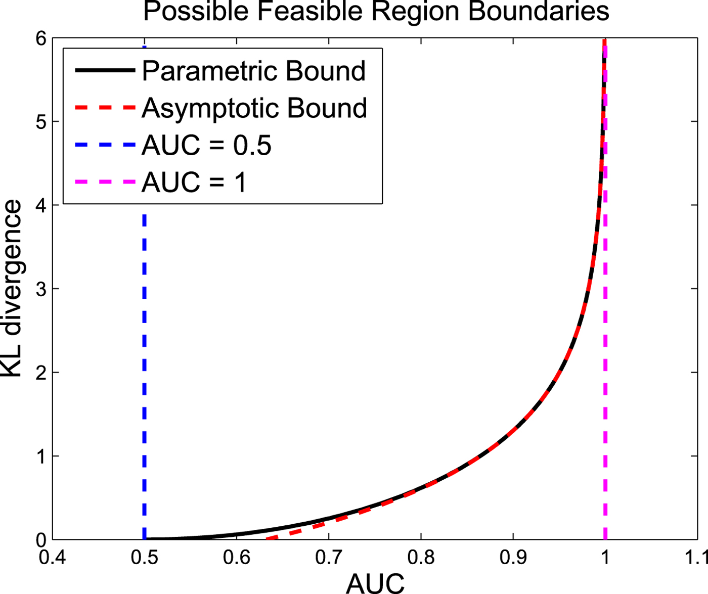
Figure 4 shows the possible feasible region and the asymptotic behavior log-scale. As it is shown in this figure, the parametric upper bound can be approximated with a straight line especially for large values of the parameter a (the result in Proposition ??). Also, Fig. 5 shows the possible feasible region and the asymptotic behavior in regular-scale.
Log-scale of the possible feasible region and its asymptotic behavior (linear line) for the AUC and the KL divergence pair for all possible detectors or equivalently all possible ROC curves (the KL divergence is between the LLRT statistics under different hypotheses, i.e.  ${\cal D}(f_{L_1}(l) || f_{L_0}(l))$ or ${\cal D}(f_{L_0}(l) || f_{L_1}(l))$.) Close-up part shows the non-linear behavior of the possible feasible region around one.

The possible feasible region boundaries and its asymptotic behavior for the AUC and the KL divergence pair for all possible detectors or equivalently all possible ROC curves (the KL divergence is between the LLRT statistics under different hypotheses, i.e.  ${\cal D}(f_{L_0}(l) || f_{L_1}(l))$ or ${\cal D}(f_{L_1}(l) || f_{L_0}(l))$.).
V. EXAMPLES AND SIMULATION RESULTS
In this section, we consider some examples of covariance matrices for Gaussian random vector X. We pick the tree structure as the graphical model corresponds to the covariance selection problem. In our simulations, we compare the numerically evaluated AUC and its lower and upper bounds and discuss their asymptotic behavior as the dimension of the graphical model, n, increases.
A) Tree approximation model
The maximum order of the lower order distributions in tree approximation problem is two, i.e. no more than pairs of variables. Let  $\underline {{X}}_{{\cal T}} \sim {\cal N} (\underline {0} ,\, {\bf \Sigma} _{\underline {{X}}_{{\cal T}}})$ have the graph representation ${\cal G}_{{\cal T}}=({\cal V},\, {\cal E}_{{\cal T}})$ where ${\cal E}_{{\cal T}} \subseteq \psi $ is a set of edges that represents a tree structure. Let $\underline {{X}}_r \sim {\cal N} (\underline {0} ,\, {\bf \Sigma} _{\underline {{X}}_r})$ have the graph representation ${\cal G}_r=({\cal V},\, {\cal E}_r)$ where ${\cal E}_r \subseteq {\cal E}_{{\cal T}}$ is the set of all edges in the graph of Xr. The joint PDF for elements of random vector Xr can be represented by joint PDFs of two variables and marginal PDFs in the following convenient form
 $$ f_{\underline{{X}}_r}(\underline{{x}}_r) = \prod_{(u,v) \in {\cal E}_r} {\displaystyle{f_{\underline{{X}}^u,\underline{{X}}^v}(\underline{{x}}^u , \underline{{x}}^v) }\over{f_{\underline{{X}}^u}(\underline{{x}}^u) f_{\underline{{X}}^v}(\underline{{x}}^v)}} \prod_{u \in {\cal V}} f_{\underline{{X}}^u}(\underline{{x}}^u).$$
Using equation (10), we can then easily construct a tree using iterative algorithms (such as the Chow-Liu algorithm [Reference Chow and Liu9] combined with the Kruskal [Reference Kruskal10] algorithm or the Prim [Reference Prim11] algorithm) by adding edges one at a time [Reference Kavcic and Moura35]. Consider the sequence of random vectors Xr with  $0\leq r \leq |{\cal E}_{{\cal T}}|$, where Xr is recursively generated by augmenting a new edge, $(i,\,j) \in {\cal E}_r$, to the graph representation of Xr−1. For the special case of Gaussian distributions, ${\bf \Sigma} _{\underline {{X}}_r}$ has the following recursive formulation [Reference Kavcic and Moura35]
 $${\bf \Sigma}_{\underline{{X}}_r}^{-1} = {\bf \Sigma}_{\underline{{X}}_{r-1}}^{-1} + {\bf \Sigma}_{i,j}^{\dagger} - {\bf \Sigma}_{i}^{\dagger} - {\bf \Sigma}_{j}^{\dagger}, \quad \forall \; 0\leq r \leq|{\cal E}_{{\cal T}}|$$
where  ${\bf \Sigma} _{i,j}^{\dagger } = [\underline {e}_i \; \underline {e}_j] {\bf \Sigma} _{i,j}^{-1} [\underline {e}_i \; \underline {e}_j]^T $ and ${\bf \Sigma} _{i}^{\dagger } = \underline {e}_i {\bf \Sigma} _{i}^{-1} \underline {e}_i^T$ where ei is a unitary vector with 1 at the i-th place and ${\bf \Sigma} _{i,j}$ and ${\bf \Sigma} _{i}$ are the 2-by-2 and 1-by-1 principle sub-matrices of ${\bf \Sigma} _{\underline {{X}}}$, with initial step ${\bf \Sigma} _{\underline {{X}}_0} = diag({\bf \Sigma} _{\underline {{X}}})$ where $diag({\bf \Sigma} _{\underline {{X}}})$ represents a diagonal matrix with diagonal elements of ${\bf \Sigma} _{\underline {{X}}}$.
Remark
For all  $0\leq r \leq |{\cal E}_{{\cal T}}|$, we have
(i)
$\hbox{tr}({\bf \Sigma} _{\underline {{X}}_r}) = \hbox{tr}({\bf \Sigma} _{\underline {{X}}}) $(ii)
$\hbox{tr}({\bf \Sigma} _{\underline {{X}}}{\bf \Sigma} _{\underline {{X}}_r}^{-1}) = n.$(iii)
${\cal D} ( f_{\underline {{X}}}(\underline {{x}}) || f_{\underline {{X}}_r}(\underline {{x}}) ) = -{1}/{2}\hbox{log}( |{\bf \Sigma} _{\underline {{X}}}{\bf \Sigma} _{\underline {{X}}_r}^{-1} |)$(iv)
$|{\bf \Sigma} _{\underline {{X}}}| \leq \ldots \leq |{\bf \Sigma} _{\underline {{X}}_r}| \leq \ldots \leq |{\bf \Sigma} _{\underline {{X}}_0}| = |diag({\bf \Sigma} _{\underline {{X}}})|$(v) H(X) ≤ … ≤ H(Xr) ≤ … ≤ H(X0)


where H(X) is differential entropy.
Tree approximation models are interesting to study since there are algorithms such as Chow-Liu [Reference Chow and Liu9] combined by the Kruskal [Reference Kruskal10] or the Prim's [Reference Prim11] that efficiently compute the model covariance matrix from the graph covariance matrix.
B) Toeplitz example
Here, we assume that the covariance matrix  $ {\bf \Sigma} _{\underline {{X}}}$ has a Toeplitz structure with ones on the diagonal elements and the correlation coefficient ρ > −(1/(n − 1)) as off-diagonal elements
 $${\bf \Sigma}_{\underline{{X}}} = \left[\matrix{ 1 & \rho & \ldots &\rho \cr \rho & \ddots & \ddots & \vdots \cr \vdots & \ddots & \ddots & \rho \cr \rho & \ldots & \rho & 1}\right].$$
For the tree structure model, all possible tree-structured distributions satisfying (10) have the same KL divergence to the original graph, i.e.  ${\cal D}( f_{\underline {{X}}}(\underline {{x}}) || f_{\underline {{X}}_{\cal T}}(\underline {{x}}))$ is constant for all possible connected tree approximation model for this example. The reason is that all the weights computed by the Chow-Liu algorithm to construct the weighted graph associated with this problem are the same and are equal to − 1/2log (1 + ρ 2), which only depends on the correlation coefficient ρ. In the sequel, we test our results for two tree structured networks: a star network and a chain network.Footnote 8
1) Star approximation
The star covariance matrix is as follows (all the nodes are connected to the first node)Footnote 9
 $${\bf \Sigma}_{\underline{{X}}_{\cal T}}^{star} = \left[\matrix{ 1 & \rho & \ldots & \ldots & \rho \cr \rho & \ddots & \rho^2 & \ldots & \rho^2 \cr \vdots & \rho^2 & \ddots & \ddots& \vdots \cr \vdots & \vdots & \ddots & \ddots & \rho^2 \cr \rho & \rho^2 & \ldots & \rho^2 & 1}\right].$$
For this example, the KL divergence and the Jeffreys divergence can be computed in closed form as
 $$\eqalign{{\cal D} (\underline{{X}}||\underline{{X}}_{star}) &= \displaystyle{1 \over 2} (n-1) \log(1+\rho)\cr &\quad - \displaystyle{1 \over 2} \log( 1 + (n-1) \rho )}$$
and
 $${\cal D}_{{\cal J}} (\underline{{X}} , \, \underline{{X}}_{star}) = \displaystyle{(n-1)(n-2) \rho^2 \over 2(1 + (n-1) \rho)}$$
respectively, where
 $${\cal D}_{{\cal J}} (\underline{{X}} , \, \underline{{X}}_{star}) = {\cal D} (\underline{{X}}||\underline{{X}}_{star}) + {\cal D} (\underline{{X}}_{star}||\underline{{X}})$$
is the Jeffreys divergence [Reference Jeffreys18]. Moreover, for large values of n, we have that
 $${\cal D} (\underline{{X}}||\underline{{X}}_{star}) \approx \displaystyle{n \over 2} \log(1+\rho)$$
and
 $${\cal D}_{{\cal J}} (\underline{{X}} , \, \underline{{X}}_{star}) \approx \displaystyle{n \over 2} \rho.$$
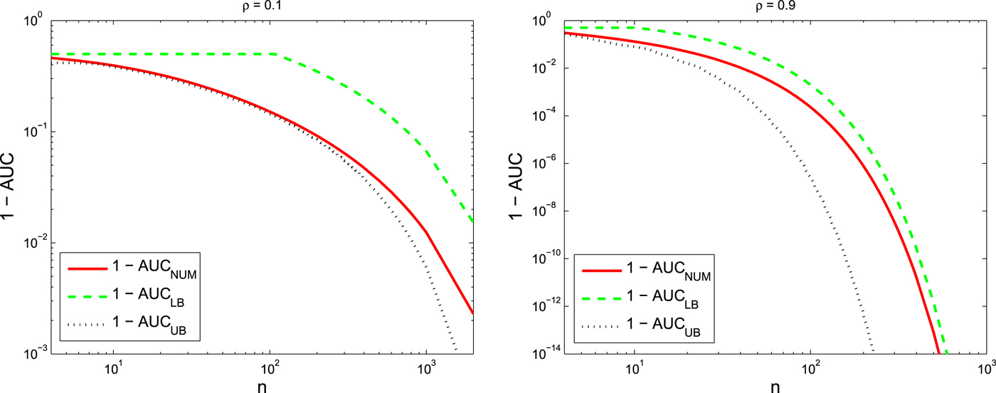
Figure 6 plots the 1 −AUC versus the dimension of the graph, n for different correlation coefficients, ρ = 0.1 and ρ = 0.9. This figure also indicates the upper bound and the lower bound for the 1 −AUC.
1 −AUC versus the dimension of the graph, n for Star approximation of the Toeplitz example with ρ = 0.1 (left) and ρ = 0.9 (right). In both figures, the numerically evaluated AUC is compared with its bounds.
2) Chain approximation
The chain covariance matrix is as follows (nodes are connected like a first order Markov chain, 1 to n)
 $${\bf \Sigma}_{\underline{{X}}_{\cal T}}^{chain} = \left[\matrix{ 1 & \rho & \rho^2 & \ldots & \rho^{n-1} \cr \rho & \ddots & \ddots & \ddots & \vdots \cr \rho^2 & \ddots & \ddots & \ddots & \rho^2 \cr \vdots & \ddots & \ddots & \ddots & \rho \cr \rho^{n-1} & \ldots & \rho^2 & \rho & 1 \cr }\right] .$$
For this example, the KL divergence and the Jeffreys divergence can be computed in closed form as
 $${\cal D} (\underline{{X}}||\underline{{X}}_{chain}) = {\cal D} (\underline{{X}}||\underline{{X}}_{star})$$
and
 $$\eqalign{&{\cal D}_{{\cal J}} (\underline{{X}} , \, \underline{{X}}_{chain}) = \displaystyle{\rho^2 \over ( 1 + (n-1) \rho )(1-\rho)}\cr & \times \left( \displaystyle{n(n-1) \over 2}- \displaystyle{n(1-\rho^n) \over 1-\rho} + \displaystyle{1-(n+1)\rho^n + n \rho^{n+1} \over (1-\rho)^2} \right)}$$
respectively. Moreover, for large values of n we have the following approximation
 $${\cal D}_{{\cal J}} (\underline{{X}} , \, \underline{{X}}_{chain}) \approx \displaystyle{n \over 2} \displaystyle{\rho \over 1 -\rho}.$$
Figure 7 plots the 1 −AUC versus the dimension of the graph, n for different correlation coefficients, ρ = 0.1 and ρ = 0.9 as well as its upper and lower bounds.
1 −AUC versus the dimension of the graph, n for Chain approximation of the Toeplitz example with ρ = 0.1 (left) and ρ = 0.9 (right). In both figures, the numerically evaluated AUC is compared with its bounds.
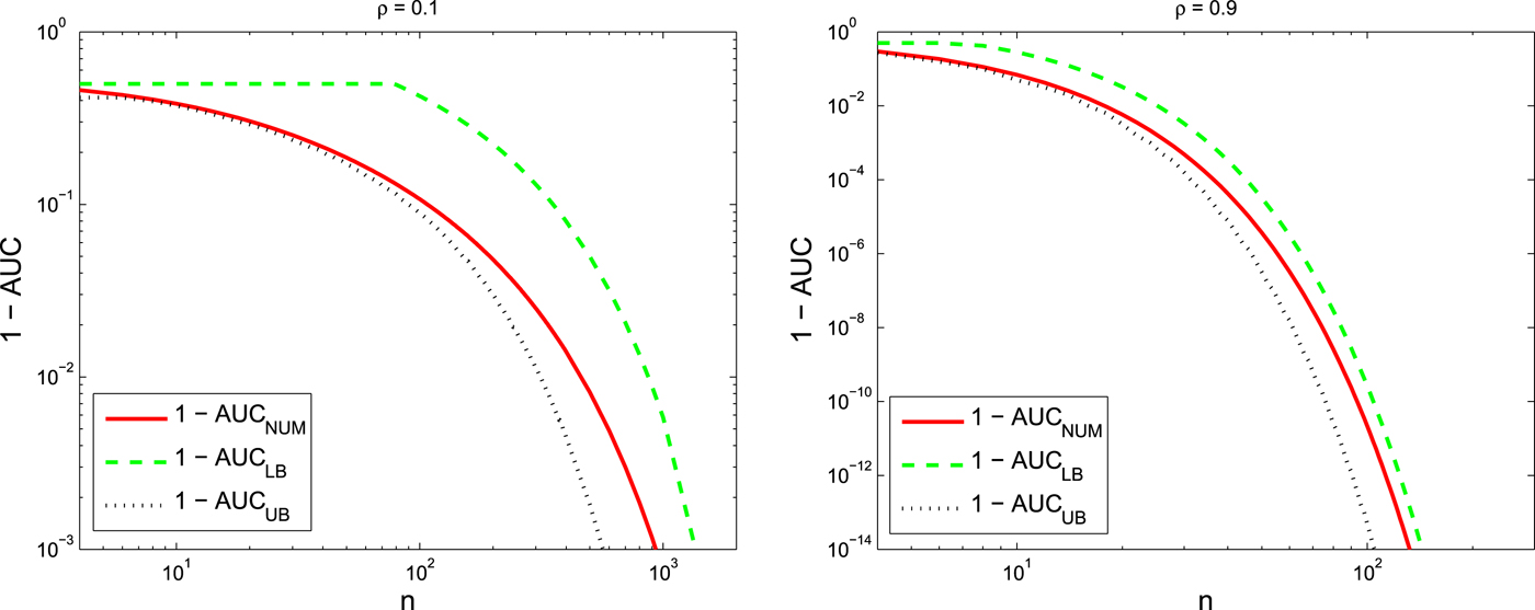
In both Figs 6 and 7,  $(1-\hbox{AUC})$ and its bounds rapidly go to 0 which means that AUC goes to one as we increase the number of nodes, n, in the graph. More precisely, bounds for $1-\hbox{AUC}$ are decaying exponentially as the dimension of the graph, n, increases which is consistent with the theory obtained for analytical bounds. Furthermore, we can conclude from these figures that a smaller ρ results in a better tree approximation, i.e. covariance matrices with smaller correlation coefficients are more like tree structure model. Moreover, comparing the AUC for the star network approximation with the AUC for the chain network approximation we conclude that the star network is a much better approximation than the chain network even though that both approximation networks have the same KL divergences. We can also interpret this fact through the analytical bounds obtained in this paper. The star network is a better approximation than the chain network since the decay rate of $1-\hbox{AUC}$ for the star network is less than its decay rate for the chain network.
Remark
The star approximation in the above example has lower AUC than the chain approximation. Practically, it means the correlation between nodes that are not connected in the approximated graphical structure gives a better approximation in the star network than the chain network.
C) Solar data
In this subsection, we look at real solar data. As discussed in the introduction, part of our motivation for this research is based on looking at distributed state estimation for microgrids with distributed renewable energy sources. Solar radiation data at these energy sources are highly correlated and we look to approximate the distribution of this data with simpler approximations that can be represented by trees. Here we see that when the number of nodes is moderately large (19) (first example) that tree approximations do not work well. However, when we have a small number of sources (6) (second example), then with the proper edge inclusion tree approximations work well.
In this Example, a covariance matrix is calculated based on datasets presented in [Reference Khajavi, Kuh and Santhanam37]. Two datasets are used from the National Renewable Energy Laboratory (NREL) website [38]. The first data set is the Oahu solar measurement grid which consists of 19 sensors (17 horizontal sensors and two tilted sensors) and the second one is the NREL solar data for 6 sites near Denver, Colorado. These two data sets are normalized using the standard normalization method and the zenith angle normalization method [Reference Khajavi, Kuh and Santhanam37] and then the unbiased estimate of the correlation matrix is computed.Footnote 10
1) The Oahu solar measurement grid dataset
From data obtained from 19 solar sensors at the island of Oahu, we computed the spatial covariance matrix during the summer season at 12:00 PM averaged over a window of 5 min. Then, the AUC and the KL divergence are computed for those tree structures that are generated using Markov Chain Monte-Carlo (MCMC) method. Figure 8 shows the distribution of those tree structures generated using MCMC method versus the KL divergence (left) and versus  $\log _{10} (1-\hbox{AUC})$
(right).Footnote 11
$\log _{10} (1-\hbox{AUC})$
(right).Footnote 11
Left: distribution of the generated trees (Normalized histogram) using MCMC versus the KL divergence and Right: distribution of the generated trees (Normalized histogram) using MCMC versus  $\log _{10} (1-\hbox{AUC})$ for the Oahu solar measurement grid dataset in summer season at 12:00 PM.

Looking back at Fig. 4, for the very small value of  $1-\hbox{AUC}$ the relationship between the KL divergence and the boundary of the possible feasible region for $-\log (1-\hbox{AUC})$ is linear. This means that if the upper bound is tight then the relationship between the KL divergence and the $-\log (1-\hbox{AUC})$ is almost linear. In Fig. 8, the maximum value of 1 −AUC for this model is < 10−3 which justifies why two distributions in Fig. 8 are scaled/mirrored of each other. Moreover, just by looking at the distribution of tree models in this example, it is obvious that most tree models have similar performance. Only a small portion of the tree models have better performance than the average tree models, but the difference is not that significant.
2) The Colorado dataset
From the solar data obtained from 6 sensors near Denver, Colorado, we computed the spatial covariance matrix during the summer season at 12:00 PM averaged over a window of 5 minutes. Then, the AUC and the KL divergence are computed for all possible tree structures. Figure 9 shows the distribution of all possible tree structures versus the KL divergence (left) and versus the AUC (right).
Left: distribution of all trees (Normalized histogram) versus the KL divergence and Right: distribution of all trees (Normalized histogram) versus the AUC for the Colorado dataset in summer season at 12:00 PM.

In the Colorado dataset, there are two sensors that are very close to each other compared with the distance between all other pairs of sensors. As a result, if the particular edge between these two sensors is in the approximated tree structure we get a smaller AUC and KL divergence compared with when that particular edge is not in the tree structure. This explains why the distribution of all trees, in this case, looks like a mixture of two distributions. This result also gives us valuable insight on how to answer the following question, “How to construct informative approximation algorithms for model selection in general.” This is an example where almost all trees that contain the particular edge between the two aforementioned sensors are good approximations while the rest of the tree models' give poor performance.
3) Two-dimensional sensor network
In this example, we create a 2D sensor network using a Gaussian kernel [Reference Rasmussen and Williams39] as follows
 $$\Sigma_{\underline{{X}}}(i,j) = \left[ e^{-{({d(i , j)^2})/({2 \sigma^2})}} \right]$$
where d(i, j) is the Euclidean distance between the i-th sensor and the j-th sensor in the 2D space. All sensors are located randomly in 2D space.Footnote 12 We set σ = 1 and generate a 2D sensor network with 20 sensors. For the 2D sensor network example, Fig. 10 shows the distribution of the generated tree structures using MCMC method versus KL divergence (left) and versus  $\log _{10} (1-\hbox{AUC})$ (right). Again we see the mirroring effect in Fig. 10 as we have an almost linear relationship between the KL divergence and $-\log (1-\hbox{AUC})$. Note that, the covariance matrix generated has one dominant eigenvalue in most cases. Furthermore, Fig. 11 plots 1 −AUC as well as its analytical upper bound and lower bound versus the dimension of the graph, n for σ = 1.3 (left) and σ = 1.8 (right). To generate this figure, we randomly generated 1000 sensor networks and then plot the averaged AUC. As we can see in this figure, the 1 −AUC and its bounds decay exponentially which is consistent with the theoretical results of this paper.
Left: Distribution of the generated trees (Normalized histogram) using MCMC versus the KL divergence and Right: distribution of the generated trees (Normalized histogram) using MCMC versus  $\log _{10} (1-\hbox{AUC})$ for the 2D sensor network example with 20 sensors and σ = 1.

1 −AUC and its bounds versus the dimension of the graph, n for σ = 1.3 (left) and σ = 1.8 (right), averaged over 1000 runs of sensor networks generated randomly.
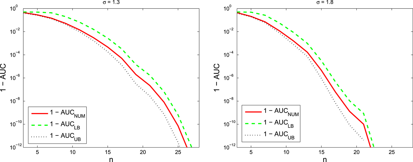
VI. CONCLUSION
In this paper, we formulate a detection problem and investigate the quality of the model selection. More specifically, we consider Gaussian distributions and discuss the covariance selection quality of a given model. We present the CAM and show its relationship with information theory divergences such as the KL divergence, the reverse KL divergence, and the Jeffreys divergence as well as the ROC curve and the area under it, i.e. the AUC, as a measure of accuracy in the detection problem framework. This paper also presents an analytical expression for the AUC that can be efficiently evaluated numerically. AUC analytical lower and upper bounds are also provided. We show that the AUC and the lower bound for the AUC depends on the eigenvalues of the CAM. Upper bounds for the AUC are obtained from finding a parametric relationship between the AUC and the KL/reverse KL divergences. We pick the tree structure as an example of an approximation model and use the Chow-Liu MST algorithm to compute the maximum likelihood tree structure approximation. Then, the quality of the Chow-Liu MST tree algorithm is investigated using the formulated detection problem. Through some examples, we show that in general, the tree approximation is not a good model as the number of nodes in the graphical model increases which is the case in high-dimensional problems such as modeling the electrical distribution grid using smart grid sensor measurements and distributed renewable energy sources. The aforementioned result is also consistent with the analytical results provided in this paper that is 1 −AUC decays exponentially as the dimension of the graph increases.
The detection framework presented in this paper can be generalized for non-Gaussian models. The AUC analytical bounds obtained in this paper can also be used in other applications that are using AUC as a relevant criterion. One example is in medicine when the AUC is used for diagnostic tests between positive instance and negative instance [Reference Johnson40] where instead of changing the coordinates we can look at the exponent of the AUC bounds. In ongoing work, we are looking at more accurate graphical approximations that involve non-tree graphs. These approximations use a variation of the CAM which we call the symmetric CAM and simple linear transformations.
ACKNOWLEDGEMENT
Portions of this paper without the theoretical justifications and detailed discussions of the detection problem was presented at the 2016 Information Theory and Application Workshop [Reference Khajavi and Kuh26]. Authors would like to thank Prof. Peter Harremoës for his helpful discussions on information divergences and assistance with Theorem 3.
FINANCIAL SUPPORT
This work was supported in part by NSF grant ECCS-1310634, the Center for Science of Information (CSoI), an NSF Science and Technology Center, under grant agreement CCF-0939370, and the University of Hawaii REIS project.
STATEMENT OF INTEREST
None.
APPENDIX
Proof of Lemma 1
The calculus-based proof for the special case of continuous PDFs is as follow. We can apply the Leibniz integral rule [Reference Flanders41] and compute the derivative of CDFs P 0(l) and P 1(l) as
 $$f_{L_0}(l) = - \displaystyle{d P_0(l) \over d l}$$
and
 $$f_{L_1}(l) = - \displaystyle{d P_1(l) \over d l}$$
since  $f_{L_0}(l)$ and $f_{L_1}(l)$ are continuous functions.Footnote 13 We have
 $$\eqalign{{\cal D} \left(f_{L_0}(l) || f_{L_1}(l)\right) &= \int_{-\infty}^{+\infty} \log \displaystyle{f_{L_0}(l) \over f_{L_1}(l)} \; f_{L_0}(l) \, dl \cr & \mathop{=}\limits^{(a)} - \int_{0}^{1} \log \displaystyle{d P_1 \over d P_0} \, d P_0 \cr & \mathop{=}\limits^{(b)} - \int_{0}^{1} \log h'(z) \, dz}$$
where equality (a) is true since we can replace PDfs  $f_{L_0}(l)$ and $f_{L_1}(l)$ using the derivative of their CDFs. Equality (b) is just a change of variable, z = P 0(l), in order to write the integral in terms of the derivative of the ROC curve. Proof for the second part of this lemma is similar to the proof of the first part.
Proof of Theorem 3
Looking back at the properties of the ROC curve, h(z), where z ∈ [0, 1], the ROC curve has to satisfy the following conditions
• C1:
$\int _{0}^{1} h'(z) dz = 1$• C2: h′(z) ≥ 0
• C3: h′(z) is decreasing

where h′(z) is the derivative of the ROC curve, h(z). Also for a given ROC curve, h(z), we can compute the AUC as
 $$\hbox{Pr} \left( L_{\Delta}>0 \right) = \int_{0}^{1} h(z) dz.$$
Then, using integration by parts, we can show that
 $$1 - \hbox{Pr} \left( L_{\Delta}>0 \right) = \int_{0}^{1} z \, h'(z) dz.$$
 To compute the possible feasible region stated in the Theorem 3, we need to optimize both of following KL divergences,  ${\cal D} (f_{L_1}(l) || f_{L_0}(l))$ and ${\cal D} (f_{L_0}(l) || f_{L_1}(l))$, with respect to the derivative of the ROC curve given a fixed AUC, $\hbox{Pr} ( L_{\Delta }>0 )$, while conditions, C1, C2, and C3 hold. To solve this optimization, we can use the method of Lagrange multiplier.
First step: Here we minimize  ${\cal D} (f_{L_1}(l) || f_{L_0}(l))$ with respect to the derivative of the ROC curve given the constraints. Optimization problem is as follow
 $$\eqalign{{\rm argmin}_{h'(z)} & - \int_{0}^{1} \log h'(z) dz \cr \hbox{s. t.} \int_{0}^{1} z \, h'(z) dz &= 1 - \hbox{Pr} \left( L_{\Delta}\gt 0 \right) \cr & \qquad\quad\hbox{C1, C2 \& C3.}}$$
To solve this optimization problem, we first write the Lagrangian. We need two coefficients a and b corresponding to conditions in optimization problem (A.1). Then, we can write the Lagrange multiplier as a function of the derivative of the ROC curve, z, a and b as follow
 $$\eqalign{& L( h'(z) , z , a , b )\cr &\quad = - \int_{0}^{1} \log h'(z) dz \cr &\qquad + a \left( \int_{0}^{1} z h'(z) dz - \left(1- \hbox{Pr} \left(L_{\Delta}>0 \right) \right) \right) \cr &\qquad + b \left( \int_{0}^{1} h'(z) dz - 1 \right).}$$
Note that, the Lagrangian, L(h′(z), z, a, b) is a convex functional [Reference Luenberger42] of h′(z). Thus, we can compute its minimum by taking its derivative with respect to h′(z). Doing so, and applying the Euler-Lagrange equation [Reference Luenberger42] we get
 $$\eqalign{\displaystyle{\delta L( h'(z) , z , a , b ) \over \delta h'(z)} & = \displaystyle{\partial L \over \partial h'} - \displaystyle{d \, \over d z}\displaystyle{\partial L \over \partial h''} \cr & = \int_{0}^{1} \left( az+b - \displaystyle{1 \over h'(z)} \right) dz.}$$
Set  $\displaystyle {\delta L( h'(z) ,\, z ,\, a ,\, b ) \over \delta h'(z)} = 0$, we get
 $$h'(z) = \displaystyle{1 \over az+b}$$
for all z ∈ [0, 1]. From C3, since h′(z) is decreasing, we can conclude that a>0. Moreover, from C1, at optimum we have  $\int _{0}^{1} h'(z) dz = 1$ and thus, we can compute one of the coefficients as $b = \displaystyle {a \over e^{a} -1}$.
Computing the AUC integral and the KL divergence using the ROC curve, we get the following parametric boundary for the possible feasible region
 $$ \hbox{Pr} ( L_{\Delta}>0 ) = \displaystyle{1 \over 1-e^{-a}} - \displaystyle{1 \over a}$$
and
 $$ {\cal D} = \log(a) + \displaystyle{a \over e^{a} - 1} - 1 - \log(1-e^{-a})$$
where  ${\cal D} = {\cal D} \left (f_{L_1}(l) || f_{L_0}(l)\right )$.
Second step: Here we minimize  ${\cal D} \left (f_{L_0}(l) ||\right .\left . f_{L_1}(l)\right )$. The Lagrange multiplier for this step is similar to the first step but it is more straightforward if we define g(η) = h −1(η). Note that using integration by parts, we can show that AUC is
 $$\hbox{Pr} ( L_{\Delta}>0 ) = \int_{0}^{1} \eta \, g'(\eta) d\eta.$$
Now, we can write the Lagrangian for the optimization problem with respect to g′(η). The Lagrangian is convex with respect to g′(η), thus taking the derivative and set it equal to zero as follow
 $$\displaystyle{\delta L( g'(\eta) , \eta , a , b ) \over \delta g'(\eta)} = 0$$
we can compute the parametric boundary for the possible feasible region. The parametric boundary, in this case, is the same as a solution in (A.3) and (A.4) with  ${\cal D} = {\cal D} (f_{L_0}(l) || f_{L_1}(l))$. Thus, combining these two steps, for the optimal boundary, we have
 $${\cal D}^{\ast}_l = \min \{ {\cal D} (f_{L_1}(l) || f_{L_0}(l)) , \, {\cal D} (f_{L_0}(l) || f_{L_1}(l)) \}.$$
Navid Tafaghodi Khajavi received B.S. degree in Electrical Engineering at Ferdowsi University, an M.S. degree in Electrical Engineering from Shahid Beheshti University, and a Ph.D. degree in Electrical Engineering from University of Hawaii at Manoa. Dr. Tafaghodi Khajavi previously worked at Shahid Beheshti University Cognitive Radio Laboratory and University of Hawaii Big Data Laboratory. He is currently working at Ford Motor Company. Dr. Tafaghodi Khajavi's research is in the area of statistical modeling and machine learning, probabilistic graphical models and big data with applications to real world problems.
Anthony Kuh received his B.S. degree in Electrical Engineering and Computer Science at the University of California, Berkeley in 1979, an M.S. degree in Electrical Engineering from Stanford University in 1980, and a Ph.D. degree in Electrical Engineering from Princeton University in 1987. Dr. Kuh previously worked at AT&T Bell Laboratories and has been on the faculty in Electrical Engineering Department at the University of Hawaii since 1986. He is currently a Professor and previously served as Department Chair. Since January, 2017 Dr. Kuh has been a program director at the National Science Foundation (NSF) in the Electrical Communications, and Cyber Systems Division. Dr. Kuh's research is in the area of neural networks and machine learning, adaptive signal processing, sensor networks, and renewable energy and smart grid applications. Dr. Kuh won an NSF Presidential Young Investigator Award, received a Distinguished Fulbright Scholar's Award working at Imperial College, London, and is an IEEE Fellow. He is currently Vice President of Technical Activities for the Asia Pacific Signal and Information Processing Association (APSIPA), is an associate editor of the APSIPA Transactions on Signal and Information Processing, and served as general co-chair of the APSIPA ASC 2018 held in Honolulu, Hawaii.


 Open access