

Warming of the climate system is unequivocal, as is now evident from observations of increases in global average air and ocean temperatures, widespread melting of snow and ice and rising global average sea level.
(IPCC, Reference Solomon, Qin, Manning, Chen, Marquis, Averyt, Tignor and Miller2007b)1. Introduction
What are the economic consequences of climate change for agriculture? What can we say about Latin American countries? According to the Fourth Assessment Report (AR4) of the IPCC, (Reference Pachauri and Reisinger2007a), in Latin America, by mid-century, increases in temperature and associated decreases in water resources are projected to lead to the gradual replacement of tropical forest by savanna in eastern Amazonia, and semi-arid vegetation will tend to be replaced by arid-land vegetation. The report also notes that there is a risk of significant reduction in water availability for agriculture and energy generation. Furthermore, the productivity of some crops as well as the livestock productivity are projected to decrease. However, the AR4 also projects an increase in soybean yields in temperate zones.
This paper studies the impact of climate change on agricultural productivity in Brazil. Brazil is an important case study for many reasons. First, it is a country where agriculture plays a key role in the national economy as well as in the international markets of agricultural commodities. Second, it has a large territory with a substantial variation in agroclimatic conditions. Not only are the long-run climate indicators quite different across regions, but also the IPCC forecasts for climate change in the country vary accordingly. Third, it is still a country where a large fraction of the rural population lives below the poverty line, with potentially high exposure risk. According to the 2000 Demographic Census, 32 per cent of the rural population lives with less than one dollar per day. Notwithstanding the positive effects of the recent redistributive policies, 14 per cent and 9.5 per cent of the rural population are characterized as poor and extremely poor, respectively, in the 2012 National Household Survey.Footnote 1 Finally, we have municipal-level data to conduct the study, which gives us almost 5,000 observations for the estimation.
We provide evidence on the effect of climate change on agricultural productivity in Brazil. Our approach is based on the estimation of a municipal-level production function in which input and crop choices provide the means of adaptation. The empirical strategy is based on a simple model of agricultural production with heterogeneity in labor skills. The model is estimated for a cross-section sample of Brazilian municipalities and simulated taking into account the IPCC projections for temperature and rainfall.
According to the IPCC, Brazil will experience an increase of 1.43°C in the average temperature and a reduction of 1.44 per cent in rainfall in the period from 2030 to 2049, which our simulations suggest will reduce the agricultural productivity by 18 per cent, with substantial heterogeneity in the different parts of the territory. The impacts on the municipalities range from −40 per cent to almost +15 per cent. The southern region of the country is expected to gain, whereas the northern and northeastern regions are expected to suffer from global warming. These results suggest that, under the current technology, climate change is likely to deepen the regional disparities across Brazilian municipalities.
Our results contribute to the literature that evaluates the consequences of climate change on agriculture in developing countries. Lybbert and Sumner, (Reference Lybbert and Sumner2012) argue that the development and diffusion of new practices in agriculture determine the capacity of farmers to mitigate and adapt to climate change. In this sense, we may observe difficulties in developing countries where agricultural productivity is relatively low, far from the technological frontier, due to lack of infrastructure or limited capital. Poverty and vulnerability in these countries are also high. Similarly, Huang et al., (Reference Huang, von Lampe and van Tongeren2011) emphasize that those production areas that are already less resilient will suffer the most because temperatures will rise further in tropical and semi-tropical latitudes.
Timmins, (Reference Timmins2006) suggests that the effects of climate change in Brazil are driven primarily by rising temperatures. Based on an endogenous land-use model, he finds that in the northeast of Brazil, warm temperatures become even warmer, making farming more difficult, whereas rising temperatures allow for a longer growing season in the south. He also observes that the effects of increasing rainfall are generally positive, except in the spring season in the southern region, where rainfall is already plentiful.
Sanghi and Mendelsohn, (Reference Sanghi and Mendelsohn2008) also present evidence of the climate change impacts on the agricultural sector in Brazil. Their estimates range from 1 to 39 per cent of annual damages, and consider the effects of global warming on net farm income and property values. A 2°C warming and 8 per cent precipitation increase scenario results in a loss of net farm income of $ 3 billion for Brazil. It is worth noting that these estimates are based on panel data of Brazilian municipalities and take into account only uniform change scenarios within the country; in practice, changes in climate may be heterogeneous in a country the size of Brazil.
In Mexico, Cohen et al., (Reference Cohen, Spring, Padilla, Paredes, Inzunza Ibarra, López and Díaz2012) report that natural disasters have increased in frequency and severity during the last few decades, leading to important economic losses in rural areas. The worsening climatic conditions affect the livelihoods and survival of numerous farmers that are dependent upon rain-fed agriculture, motivating migration flows.
In the case of India, Kumar and Gautam, (Reference Kumar and Gautam2014) suggest that the country will face more seasonal variation in temperature. Climate change represents an important threat to agriculture and food security, especially in a country where 55 per cent of the total cultivated areas do not have access to irrigation techniques. In the same direction, Sanghi and Mendelsohn, (Reference Sanghi and Mendelsohn2008) estimate a loss of 12 per cent of net farm income or $ 4 billion per year in India due to 2°C warming and an increase of 8 per cent in precipitation.
Climate change is also expected to have severe impacts in African countries, where the economic landscape depends essentially on the dynamics of climate change. The geographical location of most African countries in lower latitudes results in dramatic impacts on agriculture, forestry, energy, tourism, coastal areas and water. Countries such as Uganda, Tunisia and others have already experienced a rise in temperatures from 1 to over 3°C (Abidoye and Ayodele, Reference Abidoye and Ayodele2015).
Deressa and Hassan, (Reference Deressa and Hassan2009), in turn, emphasize the unique role of the agriculture sector in Ethiopia, where it represents approximately 50 per cent of the gross domestic product (GDP) and supports more than 80 per cent of population employment. The exposure to climate change risk is particularly important for small farms, where farmers have limited access to technology and capital. The authors estimate that even a relatively small change in temperature during winter and summer is related to a decrease of US$ 997.85 and US$ 1277.28, respectively, in net revenue per hectare. Similarly, an increase in precipitation during spring increases the net revenue per hectare by US$ 225.08, whereas increasing precipitation during winter significantly reduces net revenue by US$ 464.76.
Wood and Mendelsohn, (Reference Wood and Mendelsohn2015) also study the effects of climate change on agricultural activity in African countries. Their focus is to measure the effect of climate on agricultural net revenue on a local scale in the Fouta Djallon area of northern Guinea and southern Senegal (West Africa). The main findings show that higher temperatures and precipitation lower agricultural revenues in the economically more important rainy season, but increase revenues in the less important cool, dry season.
The remainder of the paper is organized as follows. Section 2 discusses our methodological choices based on the literature. Section 3 presents our data and section 4 provides the theoretical framework. Section 5 presents the empirical results, and concluding remarks are provided in section 6.
2. Alternative approaches to estimating the impact of climate change on agricultural production
The economic literature on the consequences of climate change is organized into two strands: the production function approach and the Ricardian approach. The first approach is the most traditional. The consequences of climate change are estimated from the association between agricultural productivity and climate measures such as temperature, rainfall or greenhouse gases levels. This association is specified as a production function in which temperature, precipitation, carbon dioxide levels and other variables are inputs (Callaway et al., Reference Callaway, Cronin, Currie and Tawil1982; Adams, Reference Adams1989; Adams et al., Reference Adams, Rosenzweig and Pearl1990). Mendelsohn et al., (Reference Mendelsohn, Nordhaus and Shaw1994, Reference Mendelsohn, Dinar, Basist and Kurukulasuriya2004, Reference Mendelsohn, Basist, Dinar, Kurukulasuriya and Williams2007a, Reference Mendelsohn, Basist, Kurukulasuriya and Dinar2007b) argue that these studies tend to overestimate the climate change damage because they ignore the capacity for adaptations that farmers can make in response to worse climatic conditions, such as the introduction of new crops, migration and occupational mobility. Conversely, the Ricardian approach assumes that land prices represent the expected present value of all net profits farmers can obtain from land (Mendelsohn et al., Reference Mendelsohn, Nordhaus and Shaw1994; Seo and Mendelsohn, Reference Seo and Mendelsohn2008a; Wood and Mendelsohn, Reference Wood and Mendelsohn2015).
Empirically, instead of studying yields of specific crops, the Ricardian approach examines how climate in different places affects the net rent or the value of farmland. Mendelsohn et al., (Reference Mendelsohn, Nordhaus and Shaw1994) explain that by directly measuring farm prices or revenues, they can estimate the direct impacts of climate on yields of different crops as well as the indirect substitution of different inputs and several kinds of potential adaptations to any climates. According to Deressa and Hassan, (Reference Deressa and Hassan2009), the most important advantage of the Ricardian model relies on its ability to take into account private adaptations. In the Ricardian model, farmers maximize profit under climate change by changing the crop mix, planting and harvesting dates, and following a host of agronomic practices.
However, Sanghi and Mendelsohn, (Reference Sanghi and Mendelsohn2008) recognize some limitations of the Ricardian approach. First of all, they emphasize that transaction costs are not taken into account, making it hard to distinguish short-term resiliency from long-term adaptation. The Ricardian approach provides a static analysis, and it does not incorporate dynamic adjustments. Second, the Ricardian approach does not take into account irrigation possibility. That might be a strong constraint of the model because agriculture heavily depends on water availability, and the climate sensitivity of rain-fed farms is indeed much higher than the climate sensitivity of irrigated farms (Kurukulasuriya et al., Reference Kurukulasuriya, Mendelsohn, Hassan and Benhin2006; Sanghi and Mendelsohn, Reference Sanghi and Mendelsohn2008; Seo and Mendelsohn, Reference Seo and Mendelsohn2008a; Wang et al., Reference Wang, Mendelsohn, Dinar, Huang, Rozelle and Zhang2008). Another important limitation of the Ricardian approach refers to the adoption of fixed prices. This assumption might lead to an overestimation of the benefits and damages of climate change, but it would not be trivial to incorporate price changes because they might be influenced by global prices (Sanghi and Mendelsohn, Reference Sanghi and Mendelsohn2008).
The choice between the two approaches is not trivial. Although the Ricardian approach accounts for a broader range of possible direct and indirect effects of climate change, it is based on the assumption that the land price is determined by the expected present value of future agricultural streams. Especially for Latin American countries, land is used not only as an agricultural input but also as a source of other benefits - ‘as a hedge against inflation, as an asset that can be liquidated to smooth consumption in the face of risk, as collateral for access to loans, as a tax shelter, or as a means of laundering illicit funds’ (de Janvry et al., Reference de Janvry, Key and Sadoulet1997). For Berry and Cline, (Reference Berry and Cline1979), ‘in countries with poorly developed capital markets, especially those with chronic inflation, landowners may prefer to hold land for speculative gain - or merely to accomplish the objective of storing of value’. Assunção (Reference Assunção2008) presents evidence compatible with the existence of a non-agricultural component of land demand, showing that land prices in Brazil increased substantially more than rental rates during periods of high macroeconomic instability.
It is also important to note that although the Ricardian approach takes adaptation into account in its measures of climate change impacts, it is not able to give insights about how farmers adapt to new climate scenarios. In this sense, Seo and Mendelsohn, (Reference Seo and Mendelsohn2008b) propose an alternative structural approach of the Ricardian model that explicitly models the underlying endogenous decisions by farmers. Seo, (Reference Seo2010, Reference Seo2015) notes that this empirical approach relies on the micro behavioral economics of global warming, that is, given the external factors such as climatic and geographic conditions, a natural resource manager is assumed to maximize the long-term profit from managing agricultural and natural resources. Thus, the theory behind this alternative model comes from a farmer's optimization decision seen as a simultaneous multiple-stage procedure. Conditional on the external factors, she/he chooses a natural resource portfolio from the full variety of portfolios available and makes decisions on the inputs and outputs of production in order to maximize the profit from the portfolio of choice. Given the profit-maximizing inputs from each farmer, it is possible to estimate the loci of profit-maximizing choices for each species across exogenous environmental factors such as temperature or precipitation (Seo and Mendelsohn, Reference Seo and Mendelsohn2008b).
The structural Ricardian analysis, or the so-called G-MAP model (short for the Geographically-scaled Microeconometric model of Adapting Portfolios in response to global warming), has already been applied to a diversity of countries and kind of farms (specialized vs. mixed). The various papers examine crops, livestock switching and specific technology adoption (such as irrigation, fertilizer and types of seeds). Seo, (Reference Seo2010), for example, investigates the adaptation portfolios in response to climate change using information on South American farmers. Kurukulasuriya and Mendelsohn, (Reference Kurukulasuriya and Mendelsohn2008), in turn, examine the impact of climate change on primary crops grown in Africa, whereas Seo and Mendelsohn, (Reference Seo and Mendelsohn2008b) study how African farmers adapt livestock management to different climatic conditions.
Following these structural Ricardian analyses, Di Falco and Veronesi, (Reference Di Falco and Veronesi2013) analyse the economic implications of different climate change adaptation strategies. In addition to investigating what is most effective – individual or collective strategies – the authors also identify the most successful strategies from a counterfactual analysis. To achieve their aim, Di Falco and Veronesi have access to a unique database on Ethiopian agriculture in which instruments are designed to study how farmers perceive climate change and adapt to new conditions. In this sense, these authors can map the full set of actual adaptation strategies implemented by individual farms. It is also worth mentioning that their empirical strategy takes into account important endogeneity issues that may lead to inconsistent estimations. Mainly, the authors estimate a multinomial endogenous switching regression model of climate change adaptation and crop net revenues using a two-stage procedure that produces selection-corrected net revenue.
Another debate in the literature is the use of climate versus weather information. The IPCC Fifth Assessment Report or AR5 (Cubasch et al., Reference Cubasch, Wuebbles, Chen, Facchini, Frame, Mahowald, Winther, Stocker, Qin, Plattner, Tignor, Allen, Boschung, Nauels, Xia, Bex and Midgley2013) emphasizes that weather describes the conditions of the atmosphere at certain places and times and takes into consideration the temperature, pressure, humidity, wind, presence of clouds, precipitation and occurrence of thunderstorms, dust storms, tornados and other special phenomena. Conversely, climate, in a narrow sense, refers to the average weather or the statistical description in terms of the mean and variability of relevant quantities, temperature, precipitation and wind over a period of time ranging from months to thousands or millions of years. The World Meteorological Organization defines a period of 30 years to average these variables and then establishes climate conditions.
Although most of the papers rely on long-run cross-section variation, based on climate data, Deschênes and Greenstone (Reference Deschênes and Greenstone2007) argue that weather variation is orthogonal to unobserved determinants of agricultural profits, which might provide consistency gains. The authors argue that estimates of any hedonic approach may confound climate with other factors and that any bias derived from omitted variables is unknown. This occurs because unmeasured characteristics, such as soil quality and the opportunity costs of the land, are important determinants of output and land values in the agricultural sector. However, the strategy of Deschênes and Greenstone (Reference Deschênes and Greenstone2007) depends largely on temporary shocks and thus does not allow for adaptation mechanisms. In this sense, it is very important to clarify that ‘climate change refers to a change in the state of the climate that can be identified (e.g., by using statistical tests) by changes in the mean and/or the variability of its properties, and that persists for an extended period, typically decades or longer’ (Cubasch et al., Reference Cubasch, Wuebbles, Chen, Facchini, Frame, Mahowald, Winther, Stocker, Qin, Plattner, Tignor, Allen, Boschung, Nauels, Xia, Bex and Midgley2013: 126).
In the same direction, Seo, (Reference Seo2013) shows that random weather fluctuations and climatic shifts are two different meteorological events and furthermore, that they have different implications for the farmers who make adaptation decisions. According to Seo, (Reference Seo2013), the panel fixed effects models, as estimated by Deschênes and Greenstone (Reference Deschênes and Greenstone2007) for example, can only reveal the impacts of random weather fluctuations on farm profits and yields, but not the impacts of climatic shifts.
One of the contributions of this paper comes from our empirical approach, which lies somewhere between the Ricardian and the production function approaches, focusing on cross-section climate variation rather than time-series weather variation. Although we explicitly specify a production function, the model from which we derive the equation for the estimation allows for adaptation in terms of the crop mix and labor mobility.
3. Data
We combine data from different sources. All variables and respective sources are shown in table 1.
Table 1. Data description

Source: Authors’ elaboration.
The information about climate comes from the Climate Research Unit (CRU) at the University of East Anglia (UEA). The information on temperature and precipitation comprises a historical average over the period from 1961 to 1990. New et al., (Reference New, Lister, Hulme and Makin2002) describe the 10’ latitude/longitude data set of mean monthly surface climate data over global land areas. In fact, the data set was built from an interpolation of station data set means for the period centered on 1961 to 1990, calculated from time series and added to the normals data set. It is important to note that the data were collected from a number of sources. In the case of South and Central America, personnel at the Centro Internacional de Agricultura Tropical (CIAT, International Center of Tropical Agriculture) have collated several thousand climatological means.Footnote 2
As noted by Randall et al., (Reference Randall, Wood, Bony, Solomon, Qin, Manning, Chen, Marquis, Averyt, Tignor and Miller2007), climate models are built on well-established physical principles and have been demonstrated to reproduce the observed features of recent climate and past climate changes. General circulation models (GCMs) give credible quantitative estimates of future climate change. GCMs are mathematical models of the general circulation of a planetary atmosphere or ocean and can be defined as spatially explicit dynamic models that simulate the three-dimensional climate system taking into account the laws of thermodynamics, momentum (Newton's second law of motion), conservation of mass and the ideal gas law (Wilby et al., Reference Wilby, Troni, Biot, Tedd, Hewitson, Smithe and Sutton2009). In this kind of model, each equation is solved at discrete points on the entire surface of the Earth and for separate layers in the atmosphere, defined by a regular grid.
According to the IPCC, (Reference Solomon, Qin, Manning, Chen, Marquis, Averyt, Tignor and Miller2007b), the atmosphere–ocean coupled GCMs (AOGCMs) are the most comprehensive climate models because they include dynamical components to describe atmospheric, ocean, land surface processes, sea ice and other components. In spite of the fact that there has been significant progress since the first IPCC report and improvements in the resolution of AOGCMs, it is worth noting that, in many cases, it is insufficient to capture the fine-scale structure of climatic variables in many regions. In such cases, the key is the regional climate models based on the empirical downscaling techniques (Christensen et al., Reference Christensen, Hewitson, Busuioc, Solomon, Qin, Manning, Chen, Marquis, Averyt, Tignor and Miller2007).
Even though the CRU also has information about climate projections, we obtain the data from the IPCC, a scientific organization set up by the World Meteorological Organization (WMO) and the United Nations Environment Programme (UNEP).Footnote 3 Our choice is based on four reasons. First of all, the models from the CRU could be considered out of date because they are based on the IPCC Third Assessment Report (TAR), not the most recent. There were significant improvements in the climate change estimates between the TAR and the Fourth Assessment Report (AR4). Second, they use only four GCMs. Third, there is false precision because the GCMs that the data set is based on all have a resolution larger than 2 degrees. Finally, only time slices for the end of the century are available.
The future scenario variables used in this paper comprise temperature and rainfall forecasts computed by the IPCC. The forecasts are based on AOGCMs and cover the period from 2030 to 2049 and consider the scenario A1B. The appendix presents detailed information regarding these models. The data are available from the IPCC as grid or raster data, with 2 degrees resolution. The forecast information for Brazil at the municipal level was built using geoprocessing toolsFootnote 4 that allow us to combine the raster data and coordinates of each Brazilian municipal seat.
The soil types were collected by Empresa Brasileira de Pesquisa Agropecuária (EMBRAPA, Brazilian Agricultural Research Institute). These variables consist of a set of 12 binary variables indicating the types of soil present in a 0.1° radius of a circumference around the center of the municipality.
Finally, the geographical coordinates (longitude, latitude and altitude) of each municipality are obtained from the Brazilian Census Bureau (IBGE), as well as our outcome variables. The agricultural output and agricultural output per hectare are averaged for the years 1997 to 2006, considering data from the Municipal Agricultural Survey (PAM) collected annually by the IBGE. We decided to consider averages to smooth out idiosyncratic shocks and thus characterize the agricultural productivity of each municipality on a longer term.
The descriptive statistics of the data are reported in table 2.
Table 2. Summary statistics

Source: Authors’ elaboration.
The temperatures in our sample of Brazilian municipalities range from 14°C to 28°C. Panel (a) of figure 1 shows that the highest average temperature levels appear at municipalities in the North and Northeast regions, which are the less developed regions in the country.

Figure 1. Average temperature and rainfall across Brazilian municipalities
The rainfall levels, as shown in table 2, range from approximately 29 to 280 mm per month. Panel (b) of figure 1 shows the geographical distribution. The Northeast region presents a large number of municipalities with low levels of precipitation.
The climate change forecasts for Brazil, derived from the IPPC projections, are depicted in figure 2. Panel (a) of figure 2 shows that the temperature is expected to increase more intensely in the North and Central-West regions. The rainfall predictions suggest an increase in precipitation in the South region and Amazônia, and a reduction in precipitation in the Central and Northeast regions (panel (b) of figure 2).

Figure 2. Predicted changes in temperature and rainfall across Brazilian municipalities
4. Theoretical framework
Consider the following Cobb–Douglas aggregate production function for each municipality i:
 $$Y_{i}=A_{i}T_{i}^{1-\alpha -\beta} K_{i}^{\alpha} L_{i}^{\beta}\exp \lpar \varepsilon_{i}\rpar ,\quad i=1,\ldots,M,$$
where Y
i
represents the total output with price normalized to 1; T
i
is the available area; K
i
and L
i
represent the amount of non-labor and labor input; A
i
is a technological factor; and $\varepsilon _{i}$
is an error term accounting for idiosyncratic determinants of the output, such as climatic shocks.
$\varepsilon _{i}$
is an error term accounting for idiosyncratic determinants of the output, such as climatic shocks.
We also assume that labor is heterogeneous – agricultural workers have different skills. A worker of type $\theta \in \lsqb 0,1\rsqb $
has productivity represented by
$\theta \in \lsqb 0,1\rsqb $
has productivity represented by $\phi \lpar \theta \rpar $
where
$\phi \lpar \theta \rpar $
where $\phi ^{\prime} >0$
and
$\phi ^{\prime} >0$
and $\phi \lpar 0\rpar =1$
. Then, the total labor input employed in a municipality i is given by:
$\phi \lpar 0\rpar =1$
. Then, the total labor input employed in a municipality i is given by:
 $$ L_{i}=\int_{0}^{1}\phi _{i}\lpar \theta \rpar L_{i}\lpar \theta \rpar d\theta,$$
where $L_{i}\lpar \theta \rpar $
is the number of workers of type θ employed in the production.
$L_{i}\lpar \theta \rpar $
is the number of workers of type θ employed in the production.
Consider now a competitive environment with no externality. For any arbitrary plot size T i , we assume that farmers in municipality i maximize the expected profit given the observed climate conditions C i :
 $$\eqalign{&\max_{K_{i},L_{i}} E\left( A_{i}T_{i}^{1-\alpha -\beta} K_{i}^{\alpha} \left( \int_{0}^{1}\phi_{i}\lpar \theta \rpar L_{i}\lpar \theta \rpar d\theta \right)^{\beta} exp \lpar \varepsilon_{i}\rpar -r_{i}K_{i}\right. \cr &\quad \left.-\int_{0}^{1}w_{i}\lpar \theta \rpar L_{i}\lpar \theta \rpar d\theta \vert C_{i}\right).}$$
The first-order conditions for $K_{i}^{\ast} $
and
$K_{i}^{\ast} $
and $L_{i}^{\ast} \lpar \theta \rpar $
,
$L_{i}^{\ast} \lpar \theta \rpar $
, $\theta \in \lsqb 0,1\rsqb $
are given by:
$\theta \in \lsqb 0,1\rsqb $
are given by:
 $$\alpha E\left( \left. {Y_{i}^{\ast} \over K_{i}^{\ast}} \right\vert C_{i} \right) = r_{i},$$
 $$\beta E\left( \left. {Y_{i}^{\ast} \over L_{i}^{\ast}} \right\vert C_{i} \right) \phi_{i}\lpar \theta \rpar = w_{i}\lpar \theta \rpar, \quad \hbox{for all} \theta \in \lsqb 0,1\rsqb. $$
The system (3)–(4) shows that the expected marginal revenue is equal to the marginal cost of each input. Moreover, equation (4) implies that ${w_{i}\lpar \theta \rpar \over \phi_{i} \lpar \theta \rpar} = {w_{i}\lpar \theta^{\prime} \rpar \over \phi_{i} \lpar \theta^{\prime} \rpar} $
for all θ,
${w_{i}\lpar \theta \rpar \over \phi_{i} \lpar \theta \rpar} = {w_{i}\lpar \theta^{\prime} \rpar \over \phi_{i} \lpar \theta^{\prime} \rpar} $
for all θ, $\theta^{\prime} \in \lsqb 0,1\rsqb $
. Thus, we have that
$\theta^{\prime} \in \lsqb 0,1\rsqb $
. Thus, we have that
 $$ w_{i}\lpar \theta \rpar = \phi_{i}\lpar \theta \rpar w_{i}\lpar 0\rpar.$$
Equation (5) shows that the wage schedule is completely determined by the baseline wage $w_{i}\lpar 0\rpar $
and the productivity function
$w_{i}\lpar 0\rpar $
and the productivity function $\phi_{i}\lpar \theta\rpar $
because workers of different abilities are substitutes. The optimal amount of non-labor and labor inputs is given by
$\phi_{i}\lpar \theta\rpar $
because workers of different abilities are substitutes. The optimal amount of non-labor and labor inputs is given by
 $$K_{i}^{\ast} = T_{i}\left({A_{i} \over r_{i}^{1 - \beta} w_{i}\lpar 0\rpar^{\beta}} \alpha^{1 - \beta} \beta^{\beta} E(exp (\varepsilon_{i})\vert C_{i})\right) ^{1 \over 1 - \alpha -\beta};$$
 $$L_{i}^{\ast} =\int_{0}^{1} \phi_{i}\lpar \theta \rpar L_{i}^{\ast} \lpar \theta \rpar d \theta = T_{i}\left({A_{i} \over r_{i}^{\alpha} w_{i} \lpar 0\rpar^{1 - \alpha}} \alpha^{\alpha} \beta^{1 - \alpha} E(exp (\varepsilon_{i})\vert C_{i})\right)^{1 \over 1-\alpha -\beta}.$$
Finally, the agricultural output for the municipality with land endowment of T i is given by
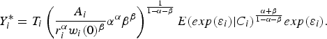 $$Y_{i}^{\ast} = T_{i}\left({A_{i} \over r_{i}^{\alpha} w_{i}\lpar 0\rpar^{\beta}} \alpha^{\alpha} \beta^{\beta} \right) ^{1 \over 1 - \alpha -\beta} E(exp (\varepsilon_{i})\vert C_{i})^{\alpha +\beta \over 1 - \alpha -\beta} exp \lpar \varepsilon_{i}\rpar. $$
In addition to the agricultural sector, we also assume there is a subsistence activity in the economy that provides a very low income $\bar{w}$
which is typically below the poverty and indigence levels of income. This subsistence activity does not require any special skill and, therefore, is available to everyone in the economy. As a consequence, it establishes a lower bound for the baseline wage rate, i.e.,
$\bar{w}$
which is typically below the poverty and indigence levels of income. This subsistence activity does not require any special skill and, therefore, is available to everyone in the economy. As a consequence, it establishes a lower bound for the baseline wage rate, i.e., $w_{i}\lpar 0\rpar \geq \bar{w}$
. This structure is commonly used in the occupational choice literature.Footnote
5
$w_{i}\lpar 0\rpar \geq \bar{w}$
. This structure is commonly used in the occupational choice literature.Footnote
5
We now adopt three assumptions to drive our empirical analysis.
Assumption A1
There is perfect capital mobility across municipalities: r i =r for all i=1, …, M.
Assumption A2
The total factor productivity is determined by a constant A and an idiosyncratic term υ
i
across municipalities that is independent from C
i
: $A_{i}=A\exp \lpar \upsilon_{i}\rpar $
.
$A_{i}=A\exp \lpar \upsilon_{i}\rpar $
.
Assumption A3
The number of unskilled workers (those with type θ=0) is large enough to assure that $w_{i}\lpar 0\rpar = \bar{w}$
for all i=1, …, M.
$w_{i}\lpar 0\rpar = \bar{w}$
for all i=1, …, M.
Assumptions A1 and A2 determine that all municipalities face the same capital return and do not present systematic technological differences. Assumption A3 captures the fact that most of the Brazilian municipalities have a significant fraction of the population living in poverty or even indigence conditions.
Assumption A3 states that the subsistence activity yields the same income in all municipalities.Footnote
6
This assumption is also adopted in Jeong and Townsend, (Reference Jeong and Townsend2007, Reference Jeong and Townsend2008). As a result, it means that migration (and its effect on the labor market) does not affect our analysis of agricultural productivity in our case. As shown by equation (5), the whole wage schedule in this case is completely determined by the productivity parameters $\phi_{i}\lpar \theta\rpar $
and the subsistence wage
$\phi_{i}\lpar \theta\rpar $
and the subsistence wage $\bar{w}$
.
$\bar{w}$
.
Under assumptions A1–A3, the direct effect of climate change on the agricultural output per hectare can be obtained by the following regression:
 $$\ln \left({Y_{i} \over T_{i}} \right) = \gamma _{0} + \gamma \lpar C_{i}\rpar +u_{i}, $$
where $\gamma_{0} \equiv {1 \over 1 - \alpha - \beta} \ln \left({A \over r^{\alpha}\bar{w}^{\beta} } \alpha^{\alpha} \beta^{\beta} \right) $
,
$\gamma_{0} \equiv {1 \over 1 - \alpha - \beta} \ln \left({A \over r^{\alpha}\bar{w}^{\beta} } \alpha^{\alpha} \beta^{\beta} \right) $
, $\gamma \lpar C_{i}\rpar \equiv {\alpha +\beta \over 1 - \alpha - \beta} \ln \lpar E(exp (\varepsilon_{i})\vert C_{i})\rpar $
and
$\gamma \lpar C_{i}\rpar \equiv {\alpha +\beta \over 1 - \alpha - \beta} \ln \lpar E(exp (\varepsilon_{i})\vert C_{i})\rpar $
and $u_{i} = \varepsilon _{i} + \upsilon_{i}$
. Specification (9) captures all of the direct effects of climate on agricultural productivity. Our dependent variable in this first exercise is the aggregate agricultural output per hectare for each municipality. Thus, we can interpret crop choice as embedded in the input choice. However, this analysis with assumptions A1–A3 ignores the effects of climate change that work through prices and technology adaptation.
$u_{i} = \varepsilon _{i} + \upsilon_{i}$
. Specification (9) captures all of the direct effects of climate on agricultural productivity. Our dependent variable in this first exercise is the aggregate agricultural output per hectare for each municipality. Thus, we can interpret crop choice as embedded in the input choice. However, this analysis with assumptions A1–A3 ignores the effects of climate change that work through prices and technology adaptation.
5. Empirical characterization
We now estimate (9) using cross-section variation from the Brazilian municipalities. The vector C i contains the available and observed variables regarding climate conditions for municipality i: temperature, rainfall and soil types. For the cases of temperature and precipitation, we consider a quadratic specification following Mendelsohn et al., (Reference Mendelsohn, Nordhaus and Shaw1994). The soil information is introduced as a set of dummy variables indicating each of the predominant soil types in each municipality.
In the estimation of the effect of climate change on agricultural productivity, through equation (9), it is important to notice that we only have simulated data for temperature and precipitation. We do not have forecasts for soil types, although soil conditions might be affected, in principle, by climate change. If we introduce it into the regression and keep it constant for the simulation, we may underestimate the effect of climate change on agricultural productivity. Conversely, part of the soil conditions are not affected by climate and, therefore, this can improve our estimates. Thus, we report our main results with and without conditioning on soil conditions. The results are reported in table 3. A comparison of the marginal effects of temperature and rainfall are presented in figure 3.

Figure 3. Marginal effect of temperature and rainfall
Table 3. Effect of climate on agricultural output per hectare

Note: Standard errors in parentheses. * significant at 10%; ** significant at 5%; *** significant at 1%.
Source: Authors’ elaboration.
As expected, the importance of temperature and rainfall decreases when we include soil dummies (in column 2) and geographical locations (in column 3). The largest change is observed with the latitude and longitude coordinates. The differences between the marginal effects with and without soil types are comparatively less important, especially if we restrict our attention to the relevant values – more than 20°C and less than 150 mm per month. Hereafter, we take the specification with soil types (column 2) as our preferred equation for agricultural productivity.
5.1. Simulations
The impact of climate change on agricultural productivity is estimated through equation (9). We now consider the vector of climate information for each municipality C i as containing information on temperature, rainfall and soil types. Then, we use the IPCC projection for temperature and rainfall for the period of 2030 to 2049 to build a different climate vector for each municipality, Ĉ i . The expected agricultural output per hectare in each municipality, under the new climate conditions, is given by:
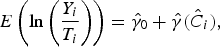 $$E\left( \ln \left({Y_{i} \over T_{i}} \right) \right) = \hat{\gamma}_{0} + \hat{\gamma} \lpar \hat{C}_{i}\rpar, $$
where $\hat{\gamma}_{0}$
and
$\hat{\gamma}_{0}$
and $\hat{\gamma}\lpar \cdot \rpar $
correspond to the estimates reported in column 2 of table 3.
$\hat{\gamma}\lpar \cdot \rpar $
correspond to the estimates reported in column 2 of table 3.
The difference in agricultural productivity due to climate change can be computed by
 $$\Delta E\left( \ln \left( {Y_{i} \over T_{i}} \right) \right) = \lpar \hat{\gamma}_{0} + \hat{\gamma} \lpar \hat{C}_{i}\rpar \rpar - \lpar \hat{\gamma}_{0} + \hat{\gamma}\lpar C_{i}\rpar \rpar, $$
where the first term is the expected agricultural output per hectare in each municipality under new climate conditions $\lpar \hat{C}_{i}\rpar $
and the second term is the expected agricultural output per hectare in each municipality under present climate conditions
$\lpar \hat{C}_{i}\rpar $
and the second term is the expected agricultural output per hectare in each municipality under present climate conditions $\lpar C_{i}\rpar $
.
$\lpar C_{i}\rpar $
.
From the predicted agricultural output per hectare, we can obtain the percentage change in agricultural productivity given by the climate change in each municipality. A map with the impact for all Brazilian municipalities is depicted in figure 4, and the results aggregated for Brazilian states, macro regions and the whole country are presented in table 4.

Figure 4. Effects of climate change on agricultural output
Table 4. Simulated effects of climate change on agricultural output her hectare

Note: The reported values are the weighted average at the state level of forecasts and simulated climate change effects at the municipal level. Simulated climate change effects at the municipal level and their confidence interval are available upon request to the authors.
Source: Authors’ elaboration.
Considering the whole country, the increase of 6.57 per cent in the average temperature along with the decrease of 0.71 per cent in rainfall leads to a reduction of 18 per cent in the agricultural productivity. We can also see that the impact is very heterogeneous in the country. The state-level impacts range from −37 per cent in Rondônia State to 1 per cent in Santa Catarina. The impact on the North is substantially higher than the impact on the South; such results coincide with the results of Timmins, (Reference Timmins2006). These estimates are also in accordance with previous results by Sanghi and Mendelsohn, (Reference Sanghi and Mendelsohn2008), which estimate annual damages in the agricultural sector in Brazil from 1 to 39 per cent.
An underlying assumption of the exercise above is the absence of technological responses to the new climate conditions. The results are predicted using the imputation of climate forecasts on current agricultural technological status. However, the cross-section comparisons across municipalities or states reveal how intense the technological gains should be to mitigate the impact of climate change in each municipality or state.
The results from the simulations suggest that climate change is likely to increase regional disparities across Brazilian states and municipalities because the most affected areas are those that already show lower productivity. The need for adaptation measures is higher in the poorer areas of Brazil.
6. Conclusion
The paper investigates the impact of climate change on agricultural productivity in Brazil. We present a simple model to guide the empirical analysis. The model is estimated and simulated taking into account IPCC predictions about temperature and rainfall. The results suggest that global warming is expected to generate significant effects in the country, but also that the impact is heterogeneous in the territory. Although the average effect is adverse, there are winners and losers in the process. Climate change is likely to increase regional disparities across Brazilian municipalities and states.
Appendix: GCMs used in the analysis
Table A1. Description of the data


