


1. Introduction
Hydraulic fractures occur naturally during ice calving, the sudden draining of glacial lakes, the formation of magma-driven dykes and sills, and the failure of dams. Hydraulic fractures are also engineered by injecting a viscous fluid into rock in the following contexts: the process of enhanced hydrocarbon recovery, enhanced geothermal production, waste remediation and disposal, preconditioning in mining, and, at a smaller scale, miniature hydraulic fractures propagated and then allowed to recede in order to determine the leak-off coefficient and the in situ stress. At the end of the injection phase, either the borehole is shut-in, or fluid from the fracture is allowed to flow back or is extracted by pumping. This paper considers the first of these injection cessation scenarios resulting in deflation of the hydraulic fractures due to fluid loss to the porous medium, which comprises three phases: continued propagation while the fluid pressure adjusts to the cessation of injection; deflation during arrest; and recession until closure. This paper focuses on the similarity solutions that emerge during the last of these phases as the fracture approaches closure.
Hitherto, hydraulic fracture research has concentrated mainly on modelling propagating hydraulic fractures to determine the evolving fracture footprint. However, there are also good reasons to model hydraulic fracture deflation and recession – in particular, to develop a rigorous model to interpret the decline in the borehole pressure after shut-in, which is used frequently to measure the leak-off coefficient or to identify the closure pressure to determine the minimum in situ stress  $\sigma _0$. Since thus far there has been no rigorous treatment of a deflating and receding hydraulic fracture, current leak-off identification assumes that the hydraulic fracture deflates with the same footprint at the time of shut-in (Nolte Reference Nolte1979; Economides & Nolte Reference Economides and Nolte2000), and for stress measurement, there is no clear way to pinpoint the closure pressure from the pressure–time record. The propagation of radially symmetric hydraulic fractures between shut-in and arrest has been subjected to rigorous study only recently by Mori & Lecampion (Reference Mori and Lecampion2021), while, to our knowledge, existing models of recession have been purely numerical and accomplished by implementing a minimum aperture constraint whose magnitude is determined arbitrarily, which can impact the solution significantly (Desroches & Thiercelin Reference Desroches and Thiercelin1993; Adachi et al. Reference Adachi, Siebrits, Peirce and Desroches2007; McClure & Horne Reference McClure and Horne2013; Mohammadnejad & Andrade Reference Mohammadnejad and Andrade2016; Zanganeh, Clarkson & Hawkes Reference Zanganeh, Clarkson and Hawkes2017). Laboratory hydraulic fracture experiments in a porous solid rely on active acoustic monitoring in order to infer the fracture front locations as the hydraulic fracture evolves (De Pater et al. Reference De Pater, Desroches, Groenenboom and Weijers1996; van Dam, de Pater & Romijn Reference van Dam, de Pater and Romijn2000). These experiments have reported expansion of the fracture footprint beyond shut-in and contraction of the footprint after arrest. However, accurate locations of the evolving fluid and fracture fronts in such experiments are extremely difficult to achieve. There is thus also a compelling need for rigorous semi-analytical solutions for deflating and receding hydraulic fractures to calibrate numerical models.
Recent research (Adachi & Detournay Reference Adachi and Detournay2008; Peirce & Detournay Reference Peirce and Detournay2008; Lecampion et al. Reference Lecampion2013; Peirce Reference Peirce2015, Reference Peirce2016; Dontsov & Peirce Reference Dontsov and Peirce2017) has established that constructing accurate and efficient numerical models for propagating hydraulic fractures benefits significantly from embedding the appropriate tip asymptote at the computational mesh scale. For advancing hydraulic fractures in rock with a non-zero toughness, the propagation criterion is based on the classic square root asymptote from linear elastic fracture mechanics (LEFM). However, depending on the dominant physical process relevant at the computational length scale, it may not be the LEFM propagation criterion that is the primary determinant of the location of the free boundary, but the asymptote corresponding to that dominant physical process. This has led to extensive research dedicated to identifying the multiscale tip asymptotes for propagating hydraulic fractures (Garagash, Detournay & Adachi Reference Garagash, Detournay and Adachi2011; Dontsov & Peirce Reference Dontsov and Peirce2015; Detournay Reference Detournay2016).
Unlike the case for propagation, there is no ‘recession criterion’, so in this paper we use local analysis in the tip region to establish that for a receding hydraulic fracture, the aperture increases linearly with distance from the tip. This linearly varying tip aperture provides the asymptote appropriate for locating the receding fracture front. In addition, the regularity of this tip behaviour motivates the development of a similarity solution in the form of a power series.
In § 2, we develop the mathematical model describing a receding hydraulic fracture. In § 3, we derive the linear recession asymptote. In § 4, we develop the similarity solution for a receding hydraulic fracture close to closure and provide a comparison to numerical solutions generated by an algorithm that incorporates the linear recession asymptote. We demonstrate the use of the sunset solution to estimate the leak-off coefficient by treating the numerical solution as a proxy for laboratory or field measurements; we also use the sunset solution to estimate the scaling of the duration of recession in terms of a dimensionless shut-in time. In § 5, we make some concluding remarks.
2. Mathematical model
2.1. Assumptions
The mathematical model describing the dynamics of a fluid-driven fracture needs to account for the dominant physical processes involved, such as: the deformation of the rock due to fracture opening; a criterion for fracture growth; a description of the fluid flow within the fracture; and the leak-off of fluid to the surrounding porous medium. In order that the model be tractable, we make the following simplifying assumptions. (i) The fracture propagates in a linear elastic solid characterized by Young's modulus  $E$ and Poisson's ratio $\nu$. (ii) Growth of the fracture is assumed to be mode I according to LEFM, and modulated by the fracture toughness $K_{Ic}$. (iii) Fluid flow within the fracture is assumed to be laminar and follows lubrication theory, while the fluid is assumed to be incompressible and Newtonian with a dynamic viscosity $\mu$. (iv) Leak-off is governed by an inverse square root relationship to the exposure time and is characterized by the leak-off coefficient $C'$; this coefficient can be interpreted either as $C'=2C_L$, where $C_L$ is the Carter leak-off coefficient applicable for a cake-building fracturing fluid (Carter Reference Carter1957), or in terms of the permeability coefficient of the host rock under conditions discussed in detail in § 4.5.5. (v) There is a uniform far-field stress $\sigma _0$ normal to the fracture plane. (vi) The solid medium is assumed to be homogeneous so that $E$,
$E$,  $\nu$, $K_{Ic}$ and $C'$ are all constant. (vii) We assume that the fluid and fracture fronts coalesce.
Since we consider only the recession dynamics of the hydraulic fracture, the fracture toughness does not enter the model explicitly. However, the homogeneity of fracture toughness, and other material parameters characterizing the solid, are relevant in that we assume that the fracture has grown symmetrically about the injection point up to the point of arrest.
2.2. Governing equations for a receding hydraulic fracture in a permeable medium
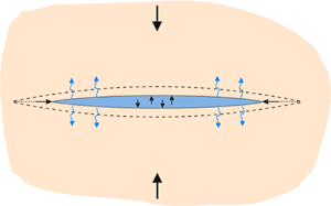
The analysis in this paper applies to two different fracture geometries: a symmetric linear fracture in a state of plane strain, which we will refer to as a KGD fracture (Khristianovic & Zheltov Reference Khristianovic and Zheltov1955; Geertsma & de Klerk Reference Geertsma and de Klerk1969; Adachi et al. Reference Adachi, Siebrits, Peirce and Desroches2007), and a planar fracture that is radially symmetric (Abé, Mura & Keer Reference Abé, Mura and Keer1976; Abé, Keer & Mura Reference Abé, Keer and Mura1979; Savitski & Detournay Reference Savitski and Detournay2002; Adachi et al. Reference Adachi, Siebrits, Peirce and Desroches2007). For the KGD fracture, the crack is in a state of plane strain as it is assumed to extend to plus and minus infinity in the out-of-plane direction perpendicular to the section shown in figure 1, while the radial fracture occupies the planar region formed by rotating the section shown in figure 1 about the axis formed by the wellbore.
Cross-section of the plane strain (KGD) and radial geometries between the wellbore and the tip.

We locate the origin of the  ${r}$-coordinate system at the injection point as shown in figure 1. The KGD fracture is confined to the line segment $r\in (-R,R)$, and because of symmetry, we need to consider only the interval $(0,R)$, where $R$ represents the fracture half-length. For the radial fracture, symmetry about the wellbore axis implies no angular dependence so the independent variable $r\in (0,R)$ describes completely the fracture's planar footprint of radius $R$. The primary unknowns in this hydraulic fracture problem are the fracture aperture $w$, the fluid pressure $p_f$ or the net pressure $p=p_f-\sigma _0$, and the fracture half-length or radius $R(t)$. It is convenient to seek a similarity solution in terms of a stretched coordinate system $s=r/R(t)$. The unknown functions in this coordinate system will be represented by lower-case symbols ${w}({s},t)$ and ${p}({s},t)$. It is also convenient to introduce a coordinate $\hat {r}$ located at the tip and pointing inwards towards the centre of the hydraulic fracture. The corresponding stretched coordinate located at the tip $s=1$ is represented by $\hat {s}=1-s$, and the unknown functions in this case are $\hat {w}(\hat {s},t)$ and $\hat {p}(\hat {s},t)$. To unify the formulae between the KGD and radial cases in the development that follows, we use a dimension parameter $\delta$ that is 1 for the KGD case and 2 for the radial case.
The solution depends on the following four alternate material parameters that are introduced to keep formulae uncluttered by unnecessary constants: the plane strain modulus  $E^{\prime }={E}/({1-\nu ^{2}})$, the alternate viscosity $\mu ^{\prime }=12\mu$, the alternate fracture toughness $K^{\prime }=( {32}/{{\rm \pi} })^{1/2}K_{Ic}$, and the leak-off coefficient $C'$. The fracture toughness is zero during recession and therefore will not enter the model equations for recession explicitly. However, since the hydraulic fracture solution at the onset of recession depends on the whole history of propagation through the history-dependent leak-off term, the receding hydraulic fracture solution will depend implicitly on the toughness and the injection rate. We will see that this history dependence attenuates as time progresses farther from the point of arrest.
2.2.1. Elasticity
For a KGD or radial fracture with radius  $R$ in an infinite homogeneous linear elastic solid, the relationship between the fracture aperture ${w}$, which is in elastic equilibrium with the imposed pressure ${p}$, can be represented (Hills et al. Reference Hills, Kelly, Dai and Korsunsky1996; Dontsov Reference Dontsov2016, Reference Dontsov2017) by an integral equation of the form
 \begin{equation} p(s,t)={-}\frac{E^{\prime }}{2{\rm \pi} R}\int_{0}^{1} M(s,s^{\prime })\,\frac{\partial w}{\partial s^{\prime }}\, {\rm d} s^{\prime}, \end{equation}
where for the symmetric KGD fracture, the kernel  $M(s,s^{\prime })$ is
 \begin{equation} M(\rho ,s)=\frac{s}{s^{2}-\rho^{2}}, \end{equation}
while for the radially symmetric fracture,  $M(s,s^{\prime })$ is given by
 \begin{equation} M(\rho ,s)=\left\{ \begin{array}{@{}ll} \displaystyle \dfrac{1}{\rho }\,K \left(\dfrac{s^{2}}{\rho^{2}}\right)+\dfrac{\rho }{s^{2}-\rho^{2}}\,E \left(\dfrac{s^{2}}{\rho^{2}}\right), & \rho >s ,\\ \displaystyle \dfrac{s}{s^{2}-\rho^{2}}\,E \left(\dfrac{s^{2}}{\rho^{2}}\right), & \rho < s , \end{array} \right. \end{equation}
where  $K(\cdot )$ and $E(\cdot )$ are complete elliptic integrals of the first and second kind, respectively.
We observe that the expression in (2.2) has been obtained from the following integral equation with a Cauchy kernel by exploiting symmetry:
 \begin{equation} p(s,t)={-}\frac{E^{\prime }}{4{\rm \pi} R}\int_{{-}1}^{1}\, \frac{\partial w}{\partial s^{\prime }}\frac{1}{s^{\prime }-s}\, {\rm d} s^{\prime }={-}\frac{E^{\prime }}{ 4{\rm \pi} R} \int_{0}^{2}\frac{\partial \hat{w}}{\partial \hat{s}^{\prime }}\, \frac{1}{\hat{s}^{\prime }-\hat{s}}\, {\rm d} \hat{s}^{\prime}.\end{equation}
Shifting to the tip coordinate  $\hat {s}$ in (2.4), the first integral reduces to the second integral.
Singularity structure of the kernel functions:
If we consider source points  $s=\rho \pm \varepsilon$ a small distance $\varepsilon$ either side of the receiving point $\rho$, and expand both kernel functions $M$ given in (2.2) and (2.3), we then observe that the dominant behaviour of both kernel functions reduce to that of the Cauchy kernel given in (2.4):
 \begin{equation} M(\rho ,\rho \pm \varepsilon )={\pm} \frac{1}{2\varepsilon }+ \cdots \sim \frac{1}{2(s-\rho )},\end{equation}
where for the KGD case the next term in the expansion is  $1/4$, and for the radial case the next term in the expansion is $O(\log (\varepsilon ))$ – both of which, upon integration over a finite interval, yield a result that is finite. Thus the dominant behaviour for the pressure field can be determined by considering the Cauchy kernels given in (2.4) and (2.5).
Given the dominant behaviour of the Cauchy kernel, we will make use of the following integral in the analysis of the pressure associated with an aperture that is a power law:
 \begin{equation} \int_{0}^{a}\frac{\hat{s}^{\kappa }}{\hat{s}-\hat{\rho}}\, {\rm d} \hat{s}=f(\hat{\rho},\kappa )\,\hat{\rho}^{\kappa }+a^{\kappa }\sum_{m=0}^{u_{\kappa }} \frac{1}{\kappa -m}\left( \frac{\hat{\rho} }{a} \right)^{m},\end{equation}
where  $f(\hat {\rho },\kappa )=-{\rm \pi} \cot ({\rm \pi} \kappa )$ and $u_{\kappa }=\infty$ for $-1<\kappa \notin \mathbb {Z}^{+}=\{ 0,1,\ldots \}$, while $f(\hat {\rho },n )=\log | ({\hat {\rho } -a})/{\hat {\rho } }|$ and $u_{n}=n-1$ for $\kappa =n\in \mathbb {Z}^{+}$. Typically, asymptotic analysis for propagating hydraulic fractures considers a semi-infinite hydraulic fracture in a state of plane strain moving at a constant velocity (Garagash et al. Reference Garagash, Detournay and Adachi2011; Dontsov & Peirce Reference Dontsov and Peirce2015). The relevant integral in that case can be obtained by letting $a\rightarrow \infty$ in (2.6), which yields the important result that a power law with $-1<\kappa <0$ is an eigenfunction of the integral operator on the left-hand side of (2.6), since the summation on the right-hand side of (2.6) vanishes. In § 3, we will see that power laws with $-1<\kappa <0$ fail to yield a dominant balance for a receding hydraulic fracture, so the eigenfunction result needs to be extended to include values of $\kappa \ge 0$. For the integral to converge for $\kappa \ge 0$, it is necessary to restrict to $a<\infty$ and to establish the dominant behaviour of the integral operator in (2.6).
2.2.2. Lubrication
By combining Poiseuille's law with the continuity equation, we obtain the lubrication equation (Savitski & Detournay Reference Savitski and Detournay2002; Dontsov Reference Dontsov2016, Reference Dontsov2017) relating  $w(s,t)$ and $p(s,t)$, which, expressed in terms of the stretched coordinate $s$, is
 \begin{equation} \frac{\partial w}{\partial t}-s\,\frac{\dot{R}}{R}\,\frac{\partial w}{\partial s}=\frac{1}{\mu^{\prime}R^{2}s^{\delta -1}}\,\frac{\partial }{\partial s} \left( s^{\delta -1}w^{3}\,\frac{\partial p}{\partial s} \right) -g(s,t), \end{equation}
where  $\delta$ is the dimension parameter defined above, which is 1 for the KGD case, and 2 for the radial case. Fluid loss to the permeable rock is assumed to follow the inverse square root leak-off model
 \begin{equation} {g}(s,t)=\frac{C'}{\sqrt{t-t_{0}({s},t)}},\end{equation}
in which  $t_{0}({s},t)$ denotes the time of first exposure of point $s$ to the fracturing fluid. After arrest, $\dot {R}\le 0$, and as a result previously unfractured rock is no longer added to the hydraulic fracture so that the leak-off term ${g}$ is no longer singular. Indeed, beyond the arrest time, ${g}$ becomes progressively more spatially uniform. Thus in order to perform a local analysis to determine the asymptotic behaviour near the tip after arrest, to first order, ${g}$ will be assumed to be spatially homogeneous in the tip region, and denoted by $\hat {g}_0(t)$.
2.2.3. Initial and boundary conditions for the receding fracture
Initial conditions: At the onset of recession  $t=t_r$, the initial conditions are
 \begin{equation} R(t_r)=R_r,\quad w(s,t_r) = w_r(s), \quad \text{where } s=r/R_r. \end{equation}
Boundary conditions: For coalescent fluid and fracture fronts, the boundary conditions at the crack tip  $s=1$ are given by zero fracture opening and zero flux conditions (see Detournay & Peirce Reference Detournay and Peirce2014)
 \begin{equation} w(1,t)=0,\quad w^{3}\,\boldsymbol{\nabla} p|_{s=1}=0. \end{equation}
3. Linear asymptote for recession  $\dot {R}<0$

Since we are interested in the behaviour of the solution near the tip, we assume power-law asymptotic solutions of the form
 \begin{equation} \hat{w}\overset{\hat{s}\rightarrow 0}{\sim }A(t)\,\hat{s}^{\lambda }. \quad \tfrac{1}{2}\leq \lambda \leq 1, \end{equation}
The lower bound restriction on  $\lambda$ is required to ensure that the elastic energy release rate at the crack tip remains finite (see Rice Reference Rice1968), while the upper bound constraint is required since the power law (3.1) cannot satisfy the lubrication and elasticity equations simultaneously if $\lambda >1$. Using (2.5) and (2.6) with $\kappa =\lambda -1$, we obtain the following expression for the leading behaviour for the tip pressure:
 \begin{equation} \hat{p}\sim \left\{ \begin{array}{@{}ll} \dfrac{AE^{\prime}\lambda }{4}\cot ({\rm \pi} \lambda)\,\hat{s}^{\lambda -1}, & \dfrac{1}{2}\leq \lambda <1, \\ \dfrac{AE^{\prime}}{4{\rm \pi}}\ln \hat{s}+C, & \lambda =1. \end{array} \right. \end{equation}
Rewriting the lubrication (2.7) in terms of the tip coordinate  $\hat {s}$, we obtain
 \begin{equation} \frac{\partial \hat{w}}{\partial t}+(1-\hat{s})\,\frac{\dot{R}}{R}\,\frac{ \partial \hat{w}}{\partial \hat{s}}=\frac{1}{\mu^{\prime }R^{2}(1-\hat{s} )^{\delta -1}}\,\frac{\partial }{\partial \hat{s}}\left( (1-\hat{s})^{\delta -1}\hat{w}^{3}\,\frac{\partial \hat{p}}{\partial \hat{s}}\right) -\hat{g}. \end{equation}
Now, for  $\frac {1}{2}\leq \lambda <1$, (3.1) and (3.2) imply that the leading behaviours of the terms in (3.3) are
 \begin{gather*} \frac{\partial \hat {w}}{\partial t}\sim \dot {A}\hat {s}^{\lambda },\\ (1-\hat {s})\frac{\dot {R}}{R}\frac{\partial \hat {w}}{\partial \hat {s}}\sim \frac{\dot {R}}{R} A\lambda \hat {s}^{\lambda -1},\\ \frac{1}{\mu ^{\prime }R^{2}(1-\hat {s})^{\delta -1}}\frac{\partial }{\partial \hat {s}} \left( (1-\hat {s})^{\delta -1}w^{3} \frac{\partial \hat {p}}{\partial \hat {s}} \right) \sim \frac{E^{\prime }A^{4}}{\mu ^{\prime }R^{3}} \lambda (\lambda \,{-}\,1) \left(\lambda - \frac {1}{2}\right)\cot ({\rm \pi} \lambda )\, \hat {s}^{4\lambda -3}\end{gather*}
and
 \[\hat {g} \sim \hat {g}_0(t).\]
Thus if  $\frac {1}{2}\leq \lambda <1$ and $\dot {R}<0$, then a dominant balance with $\hat {g}_0(t)$ is not possible since $\hat {s}^{\lambda -1}$ will become infinite. So the only admissible balance is between the second term in (3.3) and $\hat {g}_0(t)$, which yields the linear asymptote $\lambda =1$,
 \begin{equation} \hat{w}=\frac{\hat{g}_{0}}{| \dot{R}| }\,R\hat{s}=\frac{\hat{g}_{0} }{| \dot{R}| }\,\hat{r}, \end{equation}
while the first and third terms in (3.3) match at the next order. The multiscale asymptotics of deflating hydraulic fractures, which includes the linear asymptote (3.4), has been considered recently in Peirce & Detournay (Reference Peirce and Detournay2022).
To illustrate the theoretical developments that follow, we use numerical solutions for receding KGD and radial fractures, which employ the implicit moving mesh algorithms (IMMAs) described in Dontsov (Reference Dontsov2016, Reference Dontsov2017), amended to use the linear asymptote (3.4) to locate the free boundary of the receding fracture.
4. Self-similarity close to closure – the sunset solution
In this subsection, we analyse the solution for a receding fracture close to the closure time  $t_{c}$, and show that in this case the fracture aperture asymptotes to a parabolic shape.
4.1. Reverse time equations
In order to simplify the analysis, we rewrite the governing equations in terms of the reverse time  $t'=t_{c}-t$. In this case, $\dot {R}(t')>0$ for recession, and the elasticity (2.1) remains unchanged, while the signs are changed in the last two terms in (3.3). For the collapsing hydraulic fracture, the current time $t$ is assumed to be sufficiently more advanced than the initiation times active in the collapsing fracture, i.e. $t \gg t_0(s,t)$, that the leak-off term may be considered to be approximately constant, so that ${g}$ is replaced by the constant $g_{0}$. The lubrication (3.3) expressed in terms of the reverse time $t^{\prime }$ becomes
 \begin{equation} \frac{\partial \hat{w}}{\partial t^{\prime }}+(1-\hat{s})\,\frac{\dot{R}}{R}\,\frac{ \partial \hat{w}}{\partial \hat{s}}={-}\frac{1}{\mu^{\prime }R^{2}}\,\frac{\partial }{ \partial \hat{s}}\left(w^{3}\,\frac{\partial \hat{p}}{ \partial \hat{s}}\right) +\frac{(\delta-1)w^{3}}{\mu^{\prime}R^{2}(1-\hat{s})}\,\frac{\partial \hat{p}}{\partial \hat{s}}+g_{0}. \end{equation}
Note that the second term on the right-hand side of (4.1) is not present in the KGD case  $\delta =1$. We observe that these reverse time equations are equivalent to those of an inflating fracture subjected to a constant source distributed throughout its growing length.
4.2. Similarity ansatz
We look for a similarity solution to this ‘growing’ hydraulic fracture driven by an influx of fluid from a constant distributed source in terms of  $s=r/R(t^{\prime })$ by assuming a solution of the form
 \begin{equation} w(s,t^{\prime })=t^{\prime \alpha }\,W(s),\quad p(s,t^{\prime })=t^{\prime \beta }\,P(s),\quad R(t^{\prime })=\varLambda t^{\prime\gamma }. \end{equation}
Note that for the reverse time,  $t^{\prime }=0$ represents the time of closure.
4.3. Fracture volume
Define the average fracture aperture  $\bar {w}$ to be
 \begin{equation} \bar{w}=\delta\int_{0}^{1}w(s,t^{\prime})\,s^{\delta-1}\, {\rm d} s=t^{\prime\alpha }\delta\int_{0}^{1}W(s)\,s^{\delta-1}\, {\rm d} s=t^{\prime\alpha }\bar{W}. \end{equation}
The crack volume  $V_{c}$ can be expressed in terms of the similarity variables as
 \begin{equation} V_{c}(t)=\bar{w}{\rm \pi}^{\delta-1}R^{\delta}={\rm \pi}^{\delta-1} \varLambda^{\delta}t^{\prime{\alpha +\delta\gamma}}\bar{W}. \end{equation}
Since the rate of change of volume should match the rate of efflux of fluid, it follows that
 \begin{equation} \dot{V_{c}}={\rm \pi}^{\delta-1}\varLambda^{\delta} (\alpha +\delta\gamma ) t^{\prime{\alpha +\delta\gamma -1}} \bar{W}=g_{0}{\rm \pi}^{\delta-1}R^{\delta}=g_{0}{\rm \pi}^{\delta-1} \varLambda^{\delta}t^{\prime\delta\gamma }. \end{equation}
Matching powers, we obtain
 \begin{equation} \alpha =1 \quad \text{and} \quad \bar{W}= \frac{g_{0}}{1+\delta\gamma}.\end{equation}
4.4. Tip asymptotics and Taylor expansion
Now,  $w(s,t^{\prime })=\hat {w}(\hat {s},t^{\prime })=t^{\prime }\,W(s)=t^{\prime }\,W(1-\hat {s})$ and, motivated by the linear asymptote in (3.4), we assume a Taylor expansion for $W$ about $s=1$ in powers of $\hat {s}$ of the form
 \begin{equation} \hat{w}(\hat{s},t^{\prime})=t^{\prime}\sum_{n=1}^{\infty } \frac{({-}1)^{n}w_{n}}{n!}\,\hat{s}^{n},\end{equation}
where  $w_{n}=({{\rm d}^{n}W}/{{\rm d} s^{n}})| _{s =1}$ and $w_0=W(1)=0$.
Taking time and space derivatives of (4.7), the left-hand side of (4.1) can be written in the form
 \begin{equation} \frac{\partial \hat{w}}{\partial t^{\prime}}+(1-\hat{s})\,\frac{\dot{R}}{R}\,\frac{ \partial \hat{w}}{\partial \hat{s}}={-}\gamma w_{1}+\sum_{n=1}^{\infty }({-}1)^{n}\,\frac{( 1-n\gamma ) w_{n}-\gamma w_{n+1}}{n!}\,\hat{s}^{n}. \end{equation}
Using (2.6) to determine the action of the Cauchy operator on each of the terms in (4.7), we obtain the following expansion for the dominant terms in the pressure  $\hat {p}$:
 \begin{equation} \hat{p}\sim \frac{E^{\prime }t^{\prime {1-\gamma}}}{4{\rm \pi} \varLambda } \sum_{n=1}^{\infty }\frac{({-}1)^{n}w_{n}}{(n-1)!}\,\hat{\rho}^{n-1}\log \hat{\rho}.\end{equation}
Comparing (4.2a–c) and (4.9), it follows that the time exponent of the pressure  $\beta$ is given by
 \begin{equation} \beta=1-\gamma.\end{equation}
Using the expansion (4.9) for the pressure, the leading behaviour of the flux gradient can be shown to be of the form
 \begin{equation} \frac{1}{R^{2}}\,\frac{\partial }{\partial \hat{s}} \left( \frac{w^{3}}{\mu^{\prime }}\,\frac{\partial \hat{p}}{\partial \hat{s}}\right) \sim \frac{E^{\prime }t^{\prime {4-3\gamma}}}{4{\rm \pi} \mu^{\prime }\varLambda^{3}}\,( 2w_{1}^{4} \hat{s}-3w_{1}^{3}w_{2}\hat{s}^{2}\log \hat{s}+\cdots ).\end{equation}
We note that in (4.1), the leading behaviour of the additional pressure gradient term
 \[ \frac{1}{R^{2}(1-\hat {s})}\frac{{w^{3}}}{{\mu ^{\prime }}} \frac{{\partial \hat {p}}}{{\partial \hat {s}}}\sim \frac{{E^{\prime }t^{\prime {4-3\gamma }}}}{{4{\rm \pi} \mu ^{\prime }\varLambda ^{3}}} w_{1}^{4}\hat {s}^{2},\]
which appears only for the radial case  $\delta =2$, is subdominant to that in (4.11). We observe that the terms in the expansion of the flux gradient (4.11) are all of the form
 \begin{equation} \frac{t^{\prime {4-3\gamma}}}{\varLambda^{3}}\,\hat{s}^{m} ( c_{m}\log \hat{s}+d_{m}) , \end{equation}
where  $c_{m}$ and $d_{m}$ are constants. Numerical evidence suggests that as it approaches closure, the fracture accelerates rather than slowing down, which implies that $\gamma <1$. Thus in the small time limit $t^{\prime }\ll 1$, it follows that $t^{\prime {4-3\gamma }}\ll 1$ and we can neglect the flux terms on the right-hand side of (4.1). The significance of the emerging subdominance of the pressure gradient terms in (4.1) in the limit $t^{\prime }\ll 1$ is profound as it signifies a decoupling of the elastic force balance equation from the fluid conservation equation, so that essentially, the remaining dominant terms in (4.1) enforce a local kinematic condition between the fluid leak-off velocity and the rate of decrease of the aperture and radius of the receding fracture.
Now matching the powers of  $\hat {s}$ in (4.8) to the only non-zero term $g_0$ on the right-hand side of (4.1) (assuming that the flux terms are negligible on this time scale), we obtain the following value for $w_{1}$ and recursion for $w_{n}$, $n > 1$:
 \begin{equation} w_{1}={-}g_{0}/\gamma \quad \text{and} \quad w_{n+1}=\frac{( 1-n\gamma ) }{ \gamma }\,w_{n}. \end{equation}
From this recursion, it follows that
 \begin{equation} w_{n}={-}( 1-\gamma ) ( 1-2\gamma ) \ldots ( 1-( n-1) \gamma ) g_{0}/\gamma^{n}. \end{equation}
Substituting these values for  $w_{n}$ into (4.7), we obtain the following expansion:
 \begin{equation} \hat{w}(\hat{s},t^{\prime})=g_{0}t^{\prime} \left[ \frac{1}{\gamma }\,\hat{s}+\sum_{n=2}^{ \infty }\frac{({-}1)^{n+1} ( 1-\gamma ) ( 1-2\gamma ) \ldots ( 1- ( n-1 ) \gamma ) }{n!\,\gamma^{n}}\,\hat{s}^{n} \right]. \end{equation}
 Note that the power series (4.15) provides a local solution centred on the fracture tip, which converges only for  $\hat {s}<1$ and will not yield a global solution valid at the centre of the fracture $\hat {s}=1$. However, we observe from (4.15) that for $\gamma <1$, there are a countable infinity of global solutions valid for $0\le \hat {s}\le 1$, each corresponding to the reciprocals $\gamma =1/2,1/3,\ldots, 1/N,\ldots$ of the integers greater than $2$, which terminate for finite $N$ to polynomial solutions. Indeed, for $\gamma =1/N$, $N\geq 2$, the series solution (4.15) terminates after $N$ terms to yield the globally valid solution of degree $N$:
$N$:
 \begin{equation} \hat{w}(\hat{s},t^{\prime})=g_{0}t^{\prime}({-}1)^{N} [ 1-( 1-\hat{s})^{N}]. \end{equation}
 From (4.16), we observe that the solutions for  $N$ odd are aphysical since $\hat {w}(\hat {x},t)<0$, so only solutions with even powers of $N$ are admissible. Furthermore, from (4.16), we also see that all these polynomial solutions satisfy the symmetry condition $({\partial \hat {w}}/{\partial \hat {s}})(1,t) = 0$ and have $N-1$ derivatives that vanish at the centre of the fracture $\hat {s}=1$. The gradient at the fracture tip, $({\partial \hat {w}}/{\partial \hat {s}})(0,t^{\prime }) = {g_{0}t^{\prime }( -1)^{N}N}$, increases with $N$ so, of these even polynomials, the solution corresponding to $\gamma = 1/2$ is the last remaining admissible shape as the fracture approaches closure. Thus the polynomial associated with $\gamma = 1/2$ forms an attractor for the receding fracture solution, which we call the sunset solution.
4.5. The sunset solution
4.5.1. Closed-form expression for the sunset solution
The similarity solution corresponding to  $\gamma = 1/2$, when expressed as a function of $s$, is given by
 \begin{equation} w(s,t^{\prime})=g_{0}t^{\prime}( 1-s^{2}),\quad s =r/R , \quad R =\varLambda t^{\prime {1/2}}. \end{equation}
The pressure  $p$ can be determined explicitly for the KGD case by substituting (4.17) into (2.1) and using the kernel given in (2.2):
 \begin{equation} p_{KGD}(s,t)=\frac{t^{\prime}E^{\prime }g_{0}}{2{\rm \pi} R} \left[ 2+s\log \left| \frac{ 1-s}{1+s}\right| \right]. \end{equation}
Similarly, the pressure  $p$ for the radial case can be determined numerically by substituting (4.17) into (2.1) and using the kernel (2.3). For the radial sunset solution, the pressure at the wellbore $s=0$ can be shown to be
 \begin{equation} p_{rad}(0,t)=\frac{t^{\prime} E^{\prime }g_{0}}{2R}. \end{equation}
Since  $\gamma = 1/2$ for the sunset solution, it follows from (4.18), (4.19) or (4.10) that the time exponent for the pressure is $\beta =1-\gamma =1/2$. In order to close the solution to the forward problem for a receding hydraulic fracture with initial conditions (2.9a,b), the only remaining parameter to specify is the prefactor $\varLambda$ in the power law for $R$ defined in (4.2c).
In figure 2, we provide IMMA solution results (indicated by solid black curves) for a receding radial hydraulic fracture on the interval  $t \in [t_r,t_c)$, i.e. from the time of initiation of recession $t_r$ to the time of closure $t_c$. Because of its practical importance, and since the results for the KGD case are essentially similar, we choose to provide these results for only the radial case. The solution depicted in figure 2 corresponds to the dimensionless parameters $(\phi ^V,\omega )=(2,10^{-6})$ defined in § 4.6. In figure 2(a), we plot the scaled fracture radius $R/R(t_r)$ as a function of the scaled reverse time $t^{\prime }/t_r$ on a log–log scale. The dashed red line represents the log–linear regression using data points sampled near $t\sim t_c$, whose gradient is $0.49$, in close agreement with the exponent $\gamma = 1/2$ for the fracture radius of the sunset solution given in (4.17). In figure 2(b), we plot the scaled wellbore aperture $w(0,t)/w(0,t_r)$ (referenced to the left-hand vertical axis) plotted as a function of the scaled reverse time $t^{\prime }/t_r$. The dashed red line represents a linear regression using data points sampled near $t\sim t_c$. The dash-dotted blue curve (referenced to the right-hand vertical axis) represents the decaying leak-off term $g$. The horizontal dashed blue line represents the estimate of $g_0$ obtained from the gradient of the dashed red line.
(a) Plot of the scaled fracture radius  $R/R(t_r)$ (solid black) as a function of the scaled reverse time $t^{\prime }/t_r$. (b) The scaled wellbore aperture $w(0,t)/w(0,t_r)$ (solid black) referenced to the left-hand vertical axis plotted as a function of the scaled reverse time $t^{\prime }/t_r$. The decaying leak-off term g (dash-dotted blue) referenced to the right-hand vertical axis is plotted as a function of $t'/t_r$.

4.5.2. Estimating the time to closure and closing the forward problem
For the receding fracture,  $\varLambda$ will be determined by the amount of fluid in the fracture at a given radius $R$ on the way to closure. Indeed, using the initial conditions (2.9a,b), assuming that $g$ is constant over the period of recession, and using (4.4) and (4.6a,b), it is possible to obtain the following estimate of the time from the initiation of recession to closure:
 \begin{equation} t_{c}-t_r\sim \frac{\delta (2+\delta )}{2g_{0}} \int_{0}^{1}w_{r}(s)\,s^{ \delta -1}\, {\rm d} s.\end{equation}
To illustrate this estimate, consider the example shown in figure 2 and use the average value over the interval  $[t_r,t_c)$ of $g\sim 50$. We obtain the estimate $(t_c-t_r)\sim 7\times 10^{-4}$, which is close to that obtained from the numerical solution $(t_c-t_r)\sim 6.13 \times 10^{-4}$. Now $\varLambda$ can be determined from the initial radius $R_r$ and the expression for $R$ in (4.2c).
4.5.3. Estimating the leak-off coefficient $C^{\prime }$

We have seen that the solution of the forward problem comprising the coupled equations (2.1) and (2.7) subject to the initial (2.9a,b) and boundary (2.10a,b) conditions reduces, in the asymptotic limit  $t\rightarrow t_c$, to the sunset solution (4.17). However, unlike the initial conditions that define a propagating fracture, which are that $w\equiv 0$ and $R\equiv 0$ at $t=0$, the initial conditions (2.9a,b) for a receding fracture are not known a priori. Indeed, the only feasible way to establish reasonable initial conditions for $R_r$ and $w_r$ is via a numerical solution. This involves modelling a hydraulic fracture that has completed the propagation and deflation at rest phases, and is at the point of transition to recession, in order to establish the initial conditions $R_r$ and $w_r$. In addition, the history embedded in the trigger time function $t_0(s,t)$ needs to be determined in order to be able to evaluate the leak-off function $g$ during recession. From a practical point of view, none of this information can be inferred from quantities that can be measured, so it would seem that there is little practical utility in the sunset solution when posed as a forward initial–boundary value problem since it relies for its initial conditions on a numerical algorithm that, in itself, is quite adequate for determining the receding fracture solution. Thus a preliminary assessment would suggest that the primary significance of the sunset solution is that it establishes the theoretical result that this class of receding fractures reduces to a self-similar form as the fracture approaches closure.
However, the similarity solution is, by definition, an asymptotic solution determined in the limit  $t^{\prime } \rightarrow 0$, which is devoid of history dependence and is also dependent not on the detailed functional form of the aperture but rather on the radius and initial fracture volume at the start of recession, as can be seen from the estimate (4.20). It is also significant that the sunset solution emerges only because the flux term (4.11) becomes subdominant to the other terms in (4.1) in the limit $t^{\prime } \rightarrow 0$, which essentially reduces (4.1) to a local kinematic condition relating the receding aperture evolution to the leak-off function $g$. It can be seen from (4.11) that this separation of dynamics from kinematics in the decoupling of elasticity from fluid flow removes the dependence of the sunset solution on two of the four fundamental material parameters defined in § 2.1, namely, the dynamic viscosity $\mu ^{\prime }$ and plane strain modulus $E^{\prime }$. We also observe that because the receding fracture does not break new rock, the solution does not depend directly on the fracture toughness $K'$. It is this decoupling of kinematics from dynamics that is responsible for the particularly simple form of the sunset solution (4.17) and its dependence on the single material parameter $C^{\prime }$ through $g_0$.
Potentially, the isolation of the single fundamental parameter  $C^{\prime }$ by the novel sunset solution could lead to a new procedure to estimate $C^{\prime }$ from decaying aperture measurements, which has hitherto not been explored in field or laboratory experiments. We reason as follows. First, we note that since the fracture is shrinking to its initial footprint as it closes, it follows that $t_{0}({s},t)\overset {t\rightarrow t_{c}}{\rightarrow }0$ for all points within the receding fracture footprint. Thus from (2.8), we obtain the following approximation for $g_{0}$:
 \begin{equation} {g}(s,t)\sim g_{0}(t)\overset{t\rightarrow t_{c}}{\sim } \frac{C^{\prime }}{\sqrt{t}}.\end{equation}
We note that  $t$ is available readily since it is simply the time elapsed since the initiation of the fracture. As an illustration of this procedure, consider the numerical solution for the decaying fracture aperture represented by the solid black curve in figure 2(b) to be a proxy for the closing fracture aperture measurement from the field or a laboratory experiment. From the sunset solution (4.17), we see that the gradient of the dashed red line in figure 2(b) provides an estimate of the leak-off velocity close to the closure time, $g_0 \overset {t\rightarrow t_{c}}{\approx }34$, whose value is illustrated by the horizontal dashed blue line referenced to the right-hand axis in that figure. The closure time in this case is $\sqrt {t_c} \sim 2.9 \times 10^{-2}$, which along with (4.21) enables us to obtain the estimate
 \begin{equation} C^{\prime }\approx g_{0}(t_{c})\,\sqrt{t_{c}}=0.986.\end{equation}
Comparing the estimate provided in (4.22) with the value of  $C^{\prime }=1$ used to generate the numerical solution, we see that the error in the estimate of $C^{\prime }$ provided by the sunset solution is less than $2\,\%$.
4.5.4. Asymptotic estimate for the radius $R(t')$

If the wellbore fluid pressure is also monitored (and it is assumed that the far-field stress  $\sigma _0$ was known from the closure pressure) and one knows $g_0(t_c)$ from the aperture closure measurements, then (4.18) and (4.19) also provide the following a posteriori asymptotic estimate for the decaying fracture length/radius $R$:
$R$:
 \begin{equation} R(t^{\prime })\sim \frac{t^{\prime }E^{\prime }\,g_{0}(t_{c})}{2^{\delta -1} {\rm \pi}^{2-\delta}\,p(0,t^{\prime })}. \end{equation}
4.5.5. Order of magnitude estimate for the permeability $k$

As mentioned in § 2.1, the leak-off coefficient  $C'$ has a dual interpretation. For a cake-building fracturing fluid, $C'$ is twice the classical Carter's leak-off coefficient $C_{L}$, but for Newtonian fluids (such as water) that do not plug the pores of the rock, $C'$ can be interpreted in terms of the rock permeability. This interpretation requires that the diffusion length – the thickness of the region adjacent to the fracture wall where the pore pressure is perturbed from its initial or far-field value $p_{0}$ – is small compared to the fracture dimension. Indeed, the early-time solution of the diffusion equation indicates that $C'$ can then be expressed as
 \begin{equation} C'=\frac{2k(\sigma_{0}-p_{0})}{\mu\sqrt{{\rm \pi} c}},\end{equation}
since the net pressure  $p_{f}-\sigma _{0}$ is small compared to $\sigma _{0}-p_{0}$, so that $p_{f}-p_{0}\approx \sigma _{0}-p_{0}$. In the above expression, $k$ is the intrinsic permeability of the rock, $\mu$ is the viscosity of the fracturing fluid assumed to be the same as the viscosity of the pore fluid, and $c$ is the diffusivity coefficient. Noting that $c$ can be written as $k/\mu S$, where $S$ is the storage coefficient, which can be approximated as $\phi /K_{f}$ (with $\phi$ denoting the porosity, and $K_{f}$ the bulk modulus of the fluid), the permeability $k$ can be expressed as
 \begin{equation} k=\frac{{\rm \pi} C'^{2}\mu K_{f}}{4\phi(\sigma_{0}-p_{0})^{2}}.\end{equation}
This expression provides a means to estimate the permeability  $k$ from $C'$, if the other parameters in (4.25) can be estimated. It must be remembered that the permeability varies by many orders in rocks, and that a realistic expectation is that this procedure will result in only an order of magnitude estimate for $k$.
$k$.
4.6. Regimes of deflation and scaling law for the duration of recession
4.6.1. Scaling before shut-in
In this subsubsection, we consider the scalings associated with KGD and radial fractures driven to propagate by the injection of a viscous fluid at a constant rate  $Q_{0}$ having dimensions $[ {L^{1+\delta }}/{T}]$. Following Lister (Reference Lister1990), we define three pressures fundamental to the hydraulic fracture process, namely, the pressure drop due to viscous flow in the crack $p_{m}$, the pressure required to open the crack in the elastic medium $p_{e}$, and the crack extension pressure $p_{k}$, whose magnitudes scale as follows:
 \begin{equation} p_{m}\sim \frac{\mu^{\prime }R^{2-\delta }Q_{0}}{w^{3}},\quad p_{e}\sim \frac{E^{\prime }w}{R}\quad \text{and} \quad p_{k}\sim \frac{K^{\prime }}{R^{1/2}}. \end{equation}
There are also three fundamental volumes that need to be accounted for in the injection and leak-off process, namely, the injected volume  $V_{i}$, the volume of fluid contained in the fracture $V_{f}$, and the volume of fluid that has leaked off $V_{c}$, whose magnitudes scale as follows:
 \begin{equation} V_{i}\sim Q_{0}t,\quad V_{f}\sim wR^{\delta }\quad \text{and} \quad V_{c}\sim C^{\prime }\sqrt{t}\,R^{\delta }. \end{equation}
Following Detournay (Reference Detournay2016), the viscous scaling ( $m$-scaling) can be identified by requiring that $p_{m}\sim p_{e}$, while the storage scaling can be identified by requiring that $V_{i}\sim V_{f}$, from which it follows that the length/radius $R_{m}$ and aperture $w_{m}$ scales for the viscous storage scaling are given by, respectively,
 \begin{equation} R_{m}\sim \left( \frac{E^{\prime }Q_{0}^{3} t^{4}}{\mu^{\prime }}\right)^{{1}/({3\delta +3})}, \quad w_{m}\sim \left( \frac{\mu^{\prime \delta }Q_{0}^{3} t^{3-\delta }}{E^{\prime \delta }}\right)^{{1}/({3\delta +3})},\end{equation}
while the dimensionless toughness  $\mathcal {K}_{m}$ and leak-off coefficient $\mathcal {C}_{m}$ become
 \begin{align} \mathcal{K}_{m}:=\frac{p_{k}}{p_{e}}\sim \left( \frac{K^{\prime 14\delta -10}t^{2(\delta -1)}}{E^{\prime 10\delta -7}\mu^{\prime 4\delta -3} Q_{0}^{2\delta -1}}\right)^{{1}/({14\delta -10})},\quad \mathcal{C}_{m}:=\frac{V_{c}}{V_{i}}\sim \left( \frac{C^{\prime 12\delta-6}E^{\prime 3\delta -2}t^{6\delta -5}}{\mu^{\prime 3\delta -2} Q_{0}^{3\delta }}\right)^{{1}/({12\delta -6})}.\end{align}
The viscous leak-off scaling ( $\tilde {m}$-scaling) can be obtained by requiring $V_{i}\sim V_{c}$ instead of $V_{i}\sim V_{f}$, from which it follows that the length/radius $R_{\tilde {m}}$ and aperture $w_{\tilde {m}}$ scales for the viscous leak-off scaling are given by, respectively,
 \begin{equation} R_{\tilde{m}}\sim \left( \frac{Q_{0}^{2}t}{C^{\prime 2 }} \right)^{{1}/{2\delta }},\quad w_{\tilde{m}}\sim \left( \frac{\mu^{\prime 3\delta -2}Q_{0}^{3 \delta }t}{E^{\prime 3\delta -2}C^{\prime 2}}\right)^{{1}/({ 12\delta -8})}. \end{equation}
We observe from (4.29a,b) that the dimensionless toughness for a fracture driven by a constant injection rate  $Q_{0}$ is independent of time for a KGD fracture $\delta =1$, and increases with time for a radial fracture $\delta =2$. The dimensionless leak-off coefficients for both KGD and radial fractures driven by a constant injection rate $Q_{0}$ increase with time. We also observe that the transition time $t_{mk}$ from viscosity- to toughness-dominated propagation (which is valid only in the radial case $\delta =2$, since $\mathcal {K}_{m}$ is time-independent in the KGD case $\delta =1$) and the transition time $t_{m\tilde {m}}$ from viscosity-storage-dominated propagation to leak-off-dominated propagation are given by
 \begin{equation} t_{mk}=\left( \frac{E^{\prime 10\delta -7}\mu^{\prime 4\delta -3}Q_{0}^{2\delta -1}}{K^{\prime 14\delta -10}}\right)^{{1}/{2(\delta -1)}},\quad t_{m\tilde{m}}=\left( \frac{\mu^{\prime 3\delta -2}Q_{0}^{3\delta }}{ E^{\prime 3\delta -2}C^{\prime 12\delta -6}}\right)^{{1}/({6\delta -5})},\end{equation}
while the propagation regime parameter  $\phi$ (valid only for the radial case) is defined to be
 \begin{equation} \phi = \frac{t_{mk}}{t_{m\tilde{m}}} =\left(\frac{E^{\prime 11}\mu^{\prime 3}C^{\prime 4}Q_{0}}{K^{\prime 14}}\right)^{{9}/{14}}. \end{equation}
4.6.2. Scaling for a radial fracture after shut-in
In practice, the evolution of a hydraulic fracture involves propagation due to the injection of a fluid at flux  $Q_{0}$ (considered here to be constant) followed by shut-in at a certain time $t_{s}$, after which the fracture may continue to propagate (depending on the regime of propagation at shut-in) until ultimately it comes to rest either due to excessive leak-off or because the stress intensity factor has dropped below the critical fracture toughness. In the latter case, there is an arrest period during which the stress intensity factor $K$ decreases as the fracture continues to lose volume until $K=0$, at which point transition to recession is initiated and the fracture starts to recede. The appropriate scaling for the dynamics of a hydraulic fracture with a fixed injected volume $V_{0}$ can be obtained directly from those of a fracture driven by a constant flux $Q_{0}$ given in (4.28a,b) and (4.29a,b) by making the simple substitution $Q_{0}=V_{0}/t$. In this case, the length/radius $R_{m}^{V}(t)$ and aperture $w_{m}^{V}(t)$ scaling factors are given by
 \begin{equation} R_{m}^{V}(t)\sim \left( \frac{E^{\prime }V_{0}^{3}t}{\mu^{\prime }}\right) ^{{1}/({3\delta +3})}\quad \text{and} \quad w_{m}^{V}(t)\sim \left( \frac{\mu^{\prime \delta }V_{0}^{3}}{E^{\prime \delta }t^{\delta }}\right)^{{1}/({ 3\delta +3})}. \end{equation}
 Here, we have followed Mori & Lecampion (Reference Mori and Lecampion2021) and used the superscript  $V$ to denote the scaling for a fracture with a fixed injected volume $V_{0}$ at time $t$. The corresponding leak-off ( $\tilde {m}$-scaling) length/radius $R_{\tilde {m} }^{V}(t)$ and aperture $w_{\tilde {m}}^{V}(t)$ scalings for a hydraulic fracture with a fixed injected volume $V_{0}$ are
 \begin{equation} R_{\tilde{m}}^{V}(t)\sim \left( \frac{V_{0}^{2}}{C^{\prime 2 }t}\right)^{{1}/{2\delta }}\quad \text{and} \quad w_{\tilde{m}}^{V}(t)\sim \left( \frac{\mu^{\prime 3\delta -2}V_{0}^{3\delta }}{E^{\prime 3\delta -2}C^{\prime 2}t^{3\delta -1}} \right)^{{1}/({12\delta -8})}. \end{equation}
The dimensionless toughness and leak-off parameters for a hydraulic fracture with a fixed injected volume  $V_{0}$ are $\mathcal {K} _{m}^{V}(t)=( {t}/{t_{mk}^{V}})^{({4\delta -3})/({14\delta -10})}$ and $\mathcal {C}_{m}^{V}(t)=( {t}/{t_{m\tilde {m}}^{V}} )^{({9\delta -5})/({12\delta -6})}$, where
 \begin{align} t_{mk}^{V}=\left( \frac{\mu^{\prime 4\delta -3}E^{\prime 10\delta -7}V_{0}^{2\delta -1}}{K^{\prime 14\delta -10}}\right)^{{1}/({4\delta -3})}\quad \text{and} \quad t_{m\tilde{m}}^{V}=\left( \frac{\mu^{\prime 3\delta -2}V_{0}^{3\delta }}{E^{\prime 3\delta -2}C^{\prime 12\delta -6}}\right)^{{1}/({9\delta -5})}. \end{align}
 We define the following arrest regime parameter  $\phi ^{V}$ for KGD and radial hydraulic fractures with a fixed injected volume to characterize the modes of arrest:
 \begin{equation} \phi^{V}=\frac{t_{mk}^{V}}{t_{m\tilde{m}}^{V}}= \left( \frac{\mu^{\prime 2\delta +1}E^{\prime 8\delta +5}C^{\prime 4\delta +2}V_{0}}{K^{\prime 10\delta +6}}\right)^{({8\delta -7})/({61\delta -57})}.\end{equation}
We observe that the parameter  $\phi ^{V}$ defined in (4.36) has no meaning in the zero toughness case since $t_{mk}^{V}=\infty$.
4.6.3. Characteristic power law for the duration of recession
Since recession does not depend directly on the rock toughness  $K^{\prime }$, we expect the recession phase to be largely independent of $\phi ^{V}$. Because the recession process that we consider is driven by leak-off, which persists through propagation, arrest and recession, we choose to define the dimensionless shut-in time $\omega$ as the ratio of the shut-in time $t_{s}$ to the storage–leak-off transition time $t_{m\tilde {m}}$, i.e.
 \begin{equation} \omega =\frac{t_{s}}{t_{m\tilde{m}}} .\end{equation}
Now making use of (4.31a,b) and (4.35a,b), the following relationship can be established between the fixed injected volume transition time  $t_{m\tilde {m}}^{V}$ and the constant injection rate storage–leak-off transition time $t_{m\tilde {m}}$ in terms of the dimensionless shut-in parameter $\omega$:
 \begin{equation} t_{m\tilde{m}}^{V}=t_{m\tilde{m}}\omega^{{3\delta }/({9\delta -5})} =t_{s}\omega^{({5-6\delta })/({9\delta -5})}, \end{equation}
where the second relationship in (4.38) comes directly from the definition of  $\omega$.
Modes of arrest and recession: Using (4.38) and (4.36), we now characterize the way in which the arrest time  $t_a$ and recession time $t_r$ are impacted by the relative magnitudes of $\phi ^{V}$ and $\omega$.
(i) Consider
$\phi ^{V}\ll 1$.
(a) If
$\omega \ll 1$, then it follows from (4.38) and (4.36) that
(4.39)so after shut-in, arrest will be determined by\begin{equation} t_{s}\ \&\ t_{mk}^{V}\ll t_{m\tilde{m}}^{V}\ll t_{m\tilde{m}}, \end{equation}$t_{a}\sim t_{mk}^{V}$, and recession will be determined by $t_{r}\sim t_{m\tilde {m}}^{V}$.(b) If
$\omega \gg 1$, then it follows from (4.38) and (4.36) that
(4.40)so after shut-in, arrest and recession will be determined by\begin{equation} t_{m\tilde{m}}\ \&\ t_{mk}^{V}\ll t_{m\tilde{m}}^{V}\ll t_{s}, \end{equation}$t_{a}\sim t_{r}\sim t_{s}$.
(ii) Consider
$\phi ^{V}\gg 1$.
(a) If
$\omega \ll 1$, then it follows from (4.38) and (4.36) that
(4.41)so after shut-in, arrest and recession will be determined by\begin{equation} t_{s}\ll t_{m\tilde{m}}^{V}\ll t_{m\tilde{m}}\ \&\ t_{mk}^{V}, \end{equation}$t_{m \tilde {m}}^{V}$, i.e. $t_{a}\sim t_{r}\sim t_{m\tilde {m}}^{V}$.(b) If
$\omega \gg 1$, then it follows from (4.38) and (4.36) that
(4.42)so after shut-in, arrest and recession will be determined by\begin{equation} t_{m\tilde{m}}\ll t_{m\tilde{m}}^{V}\ll t_{s}\ \&\ t_{mk}^{V}, \end{equation}$t_{a}\sim t_{r}\sim t_{s}$.


Typical field values of  $\phi ^V$ and $\omega$:
We have seen that the two dimensionless parameters  $\phi ^V$ and $\omega$ characterize the fracture arrest and the nature of transition to recession, respectively. To establish typical field values for these parameters, assume the following ranges of material parameters that are encountered typically in the field: $E^{\prime }\sim 1\unicode{x2013}30\ \mathrm {GPa}$, $\mu ^{\prime }\sim 10^{-2}\unicode{x2013}10 \mathrm {Pa}\ \mathrm {s}$, $C^{\prime }\sim 10^{-5}\unicode{x2013}10^{-8} \mathrm {m\ s}^{-1/2}$, $K^{\prime }\sim 0.3\unicode{x2013}3 \mathrm {MPa}\, \mathrm {m}^{1/2}$, $t_{s}\sim 3600\ \mathrm {s}$ and $Q_{0}\sim 10^{-5}\unicode{x2013}10^{-3}\ \mathrm {m}^{2}\ \mathrm {s}^{-1}$ for KGD hydraulic fractures, and $Q_{0}\sim 10^{-3}\unicode{x2013}10^{-1}\ \mathrm {m}^{3}\ \mathrm {s}^{-1}$ for radial hydraulic fractures. For these ranges of material and injection parameters, the ranges of the dimensionless parameters for KGD hydraulic fractures are $10^{-23}\lesssim \omega _{{KGD}}\lesssim 10$ and $10^{-11}\lesssim \phi _{{KGD}}^{V}\lesssim 10^{4}$, while for radial hydraulic fractures they are $10^{-10}\lesssim \omega _{{RAD}}\lesssim 3$ and $10^{-10}\lesssim \phi _{{RAD}}^{V}\lesssim 10^{4}$.
4.6.4. Scaling law for the duration of recession $t_{c}-t_{r}$

In this subsubsection, we use the sunset solution to provide the estimate
 \begin{equation} t_{c}-t_{r}\sim \frac{w_{r}\sqrt{t_{r}}}{C^{\prime }},\end{equation}
where  $t_{c}$ is the closure time, $t_{r}$ is the time of initiation of recession, and $w_{r}$ is an estimate of the fracture aperture at the start of recession.
Small shut-in time  $\omega \ll 1$:
Since in this limit  $t_{r}\sim t_{m\tilde {m}}^{V}$, we use (4.33a,b) to provide the estimate $w_{r}=w_{m}^{V}(t_{m\tilde {m}}^{V})\sim$ $w_{s} \omega ^{{\delta ( 6\delta -5) }/{3( \delta +1) ( 9\delta -5) }}$, where $w_{s}$ is the aperture at shut-in, which from ( 4.28a,b) has the estimate $w_{s}\sim C^{\prime }t_{m\tilde {m} }^{1/2}\omega ^{{1}/({6\delta -3})}$. Now substituting these estimates into (4.43) and using (4.38), we obtain the following scaling for the duration of recession:
 \begin{equation} t_{c}-t_{r}\overset{\omega \ll 1}{\sim } t_{m\tilde{m}} \omega^{{3\delta}/({9\delta -5})}.\end{equation}
Comparing (4.44) and (4.38), we see that  $t_{c}\sim 2t_{r}$, which implies that at the time recession starts, only some fraction (roughly half) of the fluid has leaked off, so that the time $t_{c}-t_{r}$ that the fracture takes to recede is of the same order as the time it took to get to the point of recession $t_{r}$. In order to demonstrate this further, we consider the asymptotics of the efficiency $\eta (t)$ defined to be the ratio of the volume of fluid enclosed in the fracture $V_f(t)$ at any time $t$ to the volume of fluid that has been injected into the fracture $V_i(t)$ until time $t$, i.e. $\eta (t):={V_f(t)}/{V_{i}(t)}$, where $V_{i}=Q_{0}[ t( 1-H(t-t_{s})) +t_{s}\,H(t-t_{s})]$ and $H(t)$ is the Heaviside step function. We now use (4.34a,b) to obtain the following estimate for $\eta _{r}$:
 \begin{equation} \eta _{r}\sim \frac{w_{\tilde{m}}^{V}(t_{\tilde{m}}^{V})R_{\tilde{m}}^{V}(t_{ \tilde{m}}^{V})^{\delta }}{V_{0}}=1. \end{equation}
Now, we know that  $\eta (t)<1$ for $t>0$, so the estimate $\eta _{r}= O(1)$ established in (4.45) should be interpreted as demonstrating that the efficiency at the start of recession, $\eta _r<1$, does not depend on $\omega$ for small values of $\omega$.
Large shut-in time  $\omega \gg 1$: Since in this limit $t_{r}\sim t_{s}$, we use (4.30a,b) to provide the estimate $w_{r}\sim w_{s}\sim C^{\prime }t_{m\tilde {m} }^{1/2}\omega ^{{1}/({12\delta -8})}$, where $w_{s}$ is the aperture at shut-in. Now substituting these estimates into (4.43), we obtain the following scaling for the duration of recession:
 \begin{equation} t_{c}-t_{r}\overset{\omega \gg 1}{\sim }t_{m\tilde{m}} \omega^{({6\delta -3})/({12\delta -8})}.\end{equation}
We use (4.30a,b) to obtain the following estimate for the efficiency  $\eta _{r}$:
 \begin{equation} \eta _{r}\sim \eta (t_{s})\sim \frac{w_{\tilde{m}}(t_{s})\,R_{\tilde{m} }(t_{s})^{\delta }}{V_{0}}=\omega^{({5-6\delta})/({12\delta -8})}. \end{equation}
This establishes the rate at which the efficiency at the start of recession  $\eta _r$ decreases to zero for large values of $\omega$. We also observe from (4.38), (4.46) and (4.47) that $\eta _{r}\sim \omega ^{({5-6\delta })/({12\delta -8})}\sim ({t_{c}-t_{r}})/{t_{s}}$.
Comparison of the scaling for the duration of recession with numerical results: The solid black curves in figure 3(a) indicate the duration of recession to storage–leak-off transition time ratios  $(t_c-t_r)/t_{m\tilde {m}}$ for KGD fractures $\delta =1$ all plotted as functions of $\omega$ for a range of values of the regime parameter $\phi ^{V}=10^{j}$, $j\in \{-3,-2,-1,-\frac {3}{4},-\frac {1}{2},-\frac {1}{4},0, \frac {1}{4},\frac {1}{2},\frac {3}{4},1,2,3\}$. We observe that the duration of recession in this case, $t_{c}-t_{r}$, is independent of $\phi ^V$. The dashed red line represents the log–linear regression of the case $\phi ^V=1$ using the first few data points, which has gradient $0.746$, in close agreement with the exponent $3/4$ determined by the scaling in the limit $\omega \ll 1$ given in (4.44). The scaling in the limit $\omega \gg 1$ given in (4.46) also yields the exponent $3/4$ when $\delta =1$, which is consistent with the numerical result shown in figure 3(a). The solid black curves in 3(b) indicate the duration of recession to storage–leak-off transition time ratios $(t_c-t_r)/t_{m\tilde {m}}$ for radial fractures $\delta =2$ all plotted as functions of $\omega$ for the range of values of the regime parameter $\phi ^V \in \{0.05,0.1,0.2,0.5,1,1.25, 1.5,2,3\}$. We observe that the duration of recession $t_{c}-t_{r}$ is also independent of $\phi ^V$ for this case. The dashed red line has gradient $0.46$, close to the exponent $6/13$ obtained from the small $\omega$ scaling given in (4.44) when the value $\delta =2$ is used. The dash-dotted blue line has gradient $0.54$, close to the exponent $9/16$ obtained from the large $\omega$ scaling given in (4.44) with $\delta =2$.
The solid black lines indicate the duration of recession to storage–leak-off transition time ratios  $(t_c-t_r)/t_{m\tilde {m}}$ plotted as functions of $\omega$ for a range of values of the regime parameter $\phi ^V$. The KGD case $\delta =1$ is plotted in (a), and the dashed red line represents the log–linear regression of the case $\phi ^V=1$ using the first few data points. The radial case $\delta =2$ is plotted in (b), and the dashed red and dash-dotted blue lines represent the log–linear regressions of the case $\phi ^V=1$ using the first/last few data points.

In figure 4(a), we plot the efficiency at the initiation of recession  $\eta _r$ as a function of $\omega$ for the KGD case $\delta =1$ for three selected values of the arrest regime parameter $\phi ^{V}=10^{j}$, $j\in \{-2,0, 3\}$. The curve corresponding to $\phi ^{V}=10^{-2}$ is indicated by the ${\bullet }$ symbol at the abscissa $\omega =10^{-12}$, and for the other two curves, $\eta _r$ increases with increasing $\phi ^{V}$. We observe that $\eta _r$ develops a horizontal asymptote for small values of $\omega$, which is consistent with the scaling result (4.45). A log–linear regression, sampled for the few largest values of $\omega$, yields gradient $-0.2$, which is not far from the large $\omega$ scaling estimate (4.46), which yields the exponent $-1/4$ for $\delta =1$. The underestimation of the gradient by the numerical scheme for large $\omega$ is due to the limit on the feasibility of exploring much smaller values of $\eta _r$ associated with large $\omega$ numerically, which would be required for the asymptote to become fully developed. In figure 4(b), we plot the efficiency at the initiation of recession $\eta _r$ as a function of $\omega$ for the radial case $\delta =2$ for three selected values of the arrest regime parameter $\phi ^V \in \{0.05,0.1,3\}$. The curve corresponding to $\phi ^{V}=0.05$ is indicated by the ${\bullet }$ symbol at the abscissa $\omega =10^{-7}$, and for the other two curves, $\eta _r$ increases with increasing $\phi ^{V}$. We observe that $\eta _r$ develops a horizontal asymptote for small values of $\omega$, which is consistent with the scaling result (4.45). A log–linear regression, sampled for the few largest values of $\omega$, yields gradient $-0.38$, which is not far from the large $\omega$ scaling estimate (4.46), which yields the exponent $-7/16$ for $\delta =2$. As in the KGD case, the numerical estimate for this exponent underestimates the exponent established by scaling because of the challenge in exploring values $\eta _r \ll 1$.
The efficiency  $\eta _r$ plotted as functions of $\omega$ for three selected values of the regime parameter $\phi ^V$. The KGD case $\delta =1$ is plotted in (a) for $\phi ^{V}=10^{j},\ j\in \{-2 ( \text {indicated by } {\bullet }),0, 3\}$. The radial case $\delta =2$ is plotted in (b) for $\phi ^V \in \{0.05 ( \text {indicated by } {\bullet }),0.1,3\}$.

4.7. Comparison between numerical and sunset solutions close to closure
We now compare the sunset solution to numerical solutions for receding radial fractures, which use the IMMA described in § 3. Because of the practical importance of the radial solution, and the close resemblance of the analogous KGD comparisons, we restrict the comparison presented here to the radial case alone.
To establish the numerical solution and trigger time history  $t_0(s)$ for the comparison, the fracture is allowed to propagate while driven by an inlet flux $Q_0$ that is applied at $r=0$ until the shut-in time $t_s$. After shut-in, there is no further injection of fluid and the fracture is allowed to propagate further until it arrests at the radius $R_r$. After arrest, the fracture is allowed to deflate until the stress intensity factor is $K=0$ at the critical fracture aperture $w_r$, at which point it starts to recede. Once recession starts, the numerical scheme then uses the linear asymptote (3.4) to track the fracture as it recedes until the time of closure.
In figure 5, we plot the fracture apertures  $w$, sampled at five distinct times $t\in [t_r,t_c)$ during the recession process, scaled to the maximum aperture at shut-in $w_s$, and plotted as a function of the radial coordinate $r$ scaled to $R_s$ – the hydraulic fracture radius at shut-in. To illustrate the ubiquity of the sunset solution, we provide solutions for the following values of the dimensionless parameter pair $(\phi ^V,\omega ):$ (a) $(0.05,10^{-6})$, (b) $(2,10^{-6})$, (c) $(0.05,10)$, and (d) $(2,10)$. These values have been chosen to represent very different modes of arrest and initiation of recession. The IMMA numerical solutions are indicated by the solid black curves. Each of these curves is marked by one of the symbols ${\bullet }$, ${\blacksquare}$, ${\blacklozenge}$, ${\blacktriangle }$, ${\blacktriangleright }$ at the wellbore $r=0$, which correspond to the scaled sample times $t/t_s$ given in table 1. The symbol ${\bullet }$ at the wellbore $r=0$ denotes the aperture at the onset of recession at time $t_r$.
Fracture apertures  $w$ scaled to the maximum fracture aperture at shut-in, $w_s$, as a function of $r$ scaled to the fracture radius at shut-in, $R_s$, corresponding to the following values of parameter pair $(\phi ^V,\omega )$: (a) $(0.05,10^{-6})$, (b) $(2,10^{-6})$, (c) $(0.05,10)$, and (d) $(2,10)$. In each case: the IMMA solution is denoted by the solid black curve; the sunset solution (4.17) for which $N=2$ and $\gamma =1/2$ with wellbore apertures and radii taken from the IMMA solution is indicated by the dash-dotted blue curve; the similarity solution (4.16) corresponding to $N=4$ and $\gamma =1/4$ with wellbore apertures and radii taken from the IMMA solution is represented by the curve with the black dots; the sunset solution (4.17) with $\gamma =1/2$ and coefficients $g_0$ and $\varLambda$ obtained from the IMMA solution is indicated by the dashed red curves.

The scaled sample times  $t/t_s$ corresponding to each of the markers in figure 5.

One of the objectives of figure 5 is to provide a comparison between the sunset solution (4.17) for which  $N=2$ and $\gamma =1/2$, the next physically admissible similarity solution (4.16) corresponding to $N=4$ and $\gamma =1/4$, and the IMMA numerical solution. In order to focus on a comparison between the functional forms of the two similarity solutions and the IMMA solution, for a typical sample time $t_k$, we replace the coefficient $g_0 (t_c-t_k)$ for the similarity solutions by $w_{{IMMA}}(0,t_k)$, and the radius $\varLambda (t_c-t_k)^{\gamma }$ by $R_{{IMMA}}(t_k)$. In figure 5, the sunset solution (4.17) for which $N=2$ is represented by the dash-dotted blue curves, while the next-highest-degree similarity solution (4.16) with $N=4$ is represented by the black dotted curve. We observe that as the fracture approaches closure, $t_k\rightarrow t_c$, the solid black IMMA solution and the dash-dotted blue curve corresponding to the sunset solution converge, while the fourth-degree similarity solution represented by the black dotted curve remains distinct for all sample times. This confirms that the second-degree sunset solution (4.17) is an attractor for the receding hydraulic fracture, while the higher-degree similarity solutions in (4.16) are not.
As mentioned in § 4.5.3, the sunset solution, when posed as a forward initial-value problem, has little practical value since the fundamental parameters  $g_0$ and $\varLambda$ need to be determined from a numerical solution. However, to illustrate that the sunset solution (4.17) in which the two fundamental parameters $g_0$ and $\varLambda$ have been determined from the numerical solution does indeed converge to the IMMA numerical solution as the fracture approaches closure, we use linear regression such as that used to determine the dashed red lines plotted in figure 2 to determine estimates for $g_0$ and $\varLambda$. In figure 5, dashed red curves represent the sunset solution that uses the values of $g_0$ and $\varLambda$ obtained by regression. Consistent with the dashed red lines shown in figure 2, the sunset solution overestimates the radius $R$ and underestimates the aperture $w$ at the onset of recession; however, the sunset solution and the IMMA numerical solutions converge rapidly as $t\rightarrow t_c$.
5. Summary
This paper considers the dynamics of deflating and receding KGD and radial hydraulic fractures in permeable elastic media after fluid injection has ceased. Local analysis of the coupled equations yields the linear aperture asymptote  $\hat {w}\sim \hat {s}$ appropriate for modelling receding hydraulic fractures. Similarity solutions for receding hydraulic fractures close to the point of closure are developed. Since the aperture is regular at the tip, it is possible to expand the similarity solution in a power series about this point. By choosing the decay exponent $\gamma$ of $R$ to be $\gamma =1/N$ for $N \ge 2$ a positive integer, the power series terminates to yield a countable infinity of polynomial solutions that are valid globally. The increase of the tip gradients of these polynomial solutions with their degree $N$ indicates that ultimately, the receding fractures will approach the lowest-degree admissible solution for which $\gamma =1/2$. Thus the sunset solution, comprising the second-degree similarity solution with $\gamma =1/2$, forms an attractor for receding hydraulic fractures. The characteristic asymptotic behaviour of the sunset solution, $w \overset {t\rightarrow t_c}{\sim }(t_c-t)$ and $R \overset {t\rightarrow t_c}{\sim } (t_c-t)^{1/2}$, is confirmed by numerical solutions that embed the linear recession asymptote. Sunset solutions near the closure time show close agreement with the corresponding numerical solutions, for receding fractures for a wide range of values of the dimensionless shut-in time $\omega$ and arrest regime parameter $\phi ^V$. It is also possible to use the sunset solution to estimate the time elapsed from the onset of recession to the closure time, assuming that the fracture aperture and radius at the start of recession are given. The sunset solution is also used to establish how the duration of recession scales with the dimensionless shut-in time $\omega$.
The sunset solution manifests itself as a result of a fundamental decoupling of the elastic equilibrium equation and the fluid conservation equation caused by the emerging subdominance of the pressure gradient term in the lubrication equation as the fracture approaches closure. The dominant balance of the remaining leading terms essentially reduces the lubrication equation to a local kinematic condition on the rate of decrease in fracture aperture and radius and the leak-off velocity. As a result of this decoupling of dynamics from kinematics, the sunset solution depends on only the leak-off coefficient  $C'$ – just one of the four fundamental material parameters $E'$,
$E'$,  $\mu '$, $K'$ and $C'$ that determine the evolution of a hydraulic fracture. Because the sunset solution isolates the leak-off coefficient, it affords the opportunity to estimate $C'$ from laboratory or field measurements of the declining fracture aperture, which hitherto did not exist. Using the numerical solution as a proxy for laboratory or field measurements, we demonstrate that it is possible to use the sunset solution to estimate the leak-off coefficient $C'$ to within an accuracy of $2\,\%$.
The potential opportunities for further investigation provided by the sunset solution are manifold. There are direct benefits of this special solution such as: being able to calibrate numerical algorithms that use a width constraint to model receding hydraulic fractures; and the prospect of exploring in laboratory and field experiments potential new ways to estimate the leak-off coefficient  $C'$, the asymptotic estimates for the receding fracture radius $R(t')$, and the order of magnitude estimates for the intrinsic rock permeability $k$. In addition, the simple time signature of the fracture aperture of the sunset solution $w\sim t^{\prime }$ may provide an elementary test to identify whether the fracture has intersected a fault, for example, which we would expect to have a very different signature; or the corresponding behaviour for the wellbore pressure $p\sim t^{\prime 1/2}$ may provide a new way to identify the closure pressure.
Summary of important results and definitions:
(i) Sunset solution. Let
$t^{\prime }=t_c-t$, where $t_c$ is the closure time. Then in the limit $t^{\prime }\rightarrow 0$, receding KGD ($\delta =1$) and radial ($\delta =2$) hydraulic fractures asymptote to the similarity solution whose aperture $w(s,t^{\prime })$ and wellbore pressure $p(0,t^{\prime })$ are given by
(5.1a,b)where\begin{align} w(s,t^{\prime })=g_{0}t^{\prime}( 1-s^{2}) , \quad p(0,t^{\prime })=\frac{ t^{\prime }E^{\prime }g_{0}}{2^{\delta -1} {\rm \pi}^{2-\delta }R}, \quad s=r/R, R=\varLambda t^{\prime {1/2}}, \end{align}$\varLambda$ is a parameter that can be determined, for example, if the aperture profile $w_{r}$ at the start of recession is known (see (4.20)).(ii) Estimate of
$C^{\prime }$. Assuming that using (5.1a), $g_{0}(t_{c})$ can be determined from wellbore aperture closure measurements, and $t_c$ is the elapsed time since the initiation of the fracture to the time of closure, from (4.21) we have the following formula to estimate the alternate leak-off coefficient $C^{\prime }$:
(5.2)Using this estimate of\begin{equation} C^{\prime }\approx g_{0}(t_{c})\,\sqrt{t_{c}}. \end{equation}$C'$, it is also possible to obtain an order of magnitude estimate for the rock permeability $k$ as described in § 4.5.5.(iii) A posteriori asymptotic estimate for
$R(t)$. If the wellbore fluid pressure is also monitored (and it is assumed that the far-field stress $\sigma _0$ is known from the closure pressure) and $g_{0}(t_{c})$ has been determined from the aperture closure measurements, then (5.1b) also provides the following a posteriori asymptotic estimate for the fracture radius:
(5.3)\begin{equation} R(t^{\prime })\sim \frac{t^{\prime }E^{\prime }\,g_{0}(t_{c})}{2^{\delta -1}{\rm \pi}^{2-\delta }\,p(0,t^{\prime })}. \end{equation}(iv) Dimensionless shut-in time
$\omega$ and arrest regime parameter $\phi ^V$. Assuming a constant injection rate $Q_0$ followed by a cessation of injection at a shut-in time $t_s$, we define the dimensionless shut-in time $\omega$ and arrest regime parameter $\phi ^{V}$ as
(5.4a,b)where\begin{equation} \omega =\frac{t_{s}}{t_{m\tilde{m}}}\quad \text{and} \quad \phi^{V}=\frac{t_{mk}^{V}}{ t_{m\tilde{m}}^{V}}, \end{equation}$t_{m\tilde {m}}$ is the storage–leak-off transition time defined in (4.31b), and $t_{mk}^{V}$ and $t_{m\tilde {m}}^{V}$ are the fixed injected volume viscosity–toughness and storage–leak-off transition times defined in (4.35a,b).(v) Modes of recession. It follows directly from (4.38) that the time of initiation of recession
$t_{r}$ is characterized as follows:
(5.5)\begin{equation} \left.\begin{array}{c@{}} \text{if }\omega \ll 1,\text{ then }t_{s}\ll t_{r}\sim t_{m\tilde{m} }^{V}\ll t_{m\tilde{m}}; \\ \text{if }\omega \gg 1,\text{ then }t_{m\tilde{m}}\ll t_{m\tilde{m} }^{V}\ll t_{s}\sim t_{r}. \end{array}\right\} \end{equation}(vi) Scaling of the duration of recession
$t_c-t_r$. The sunset solution (5.1a,b) can be used to establish the following scalings for the duration of recession $t_c-t_r$ and the efficiency at the start of recession $\eta _{r}$:
(5.6)\begin{equation} \left.\begin{array}{c@{}} t_{c}-t_{r}\overset{\omega \ll 1}{\sim }t_{m\tilde{m}} \omega^{{3\delta}/({9\delta -5})}\quad\text{and}\quad \eta _{r} =O(1), \\ t_{c}-t_{r}\overset{\omega \ll 1}{\sim }t_{m\tilde{m}}\omega ^{({6\delta -3})/({12\delta -8})}\quad\text{and}\quad \eta _{r} \sim \omega^{({5\delta -6})/({ 12\delta -8})} \end{array}\right\} \end{equation}


Funding
A.P. was supported by the Natural Sciences and Engineering Research Council of Canada (NSERC) (grant no. RGPIN-2015-06039). E.D. was supported by the Bennett Chair at the UMN.
Declaration of interests
The authors report no conflict of interest.


 Open access