


1 Introduction
The contact process (CP) is a model for epidemics on graphs, described by a continuous-time Markovian dynamics, in which each vertex is in one of two states: infected or healthy. Infected vertices infect each of their healthy neighbors with a constant rate
 $\lambda $
, while also healing at a constant rate
$\lambda $
, while also healing at a constant rate
 $1$
. The model was first introduced by Harris in 1974 [Reference Harris32], who studied it on the integer lattice. Since then, much work has been done to characterize the behavior of the process also on infinite trees and locally tree-like finite graphs. The focus of this line of research has been to establish phase transitions in the long-term behavior of the process, as the spreading rate
$1$
. The model was first introduced by Harris in 1974 [Reference Harris32], who studied it on the integer lattice. Since then, much work has been done to characterize the behavior of the process also on infinite trees and locally tree-like finite graphs. The focus of this line of research has been to establish phase transitions in the long-term behavior of the process, as the spreading rate
 $\lambda $
varies. A series of works [Reference Liggett46, Reference Pemantle57, Reference Stacey65] showed that the process on the infinite d-ary tree (
$\lambda $
varies. A series of works [Reference Liggett46, Reference Pemantle57, Reference Stacey65] showed that the process on the infinite d-ary tree (
 $d\ge 2$
), with an initial infection at the root, has three possible phases separated by two critical values
$d\ge 2$
), with an initial infection at the root, has three possible phases separated by two critical values
 $0<\lambda _{c,1}<\lambda _{c,2}$
: when
$0<\lambda _{c,1}<\lambda _{c,2}$
: when
 $\lambda <\lambda _{c,1}$
the process undergoes eventual extinction, when
$\lambda <\lambda _{c,1}$
the process undergoes eventual extinction, when
 $\lambda \in (\lambda _{c,1}, \lambda _{c,2})$
there is “global but not local” survival, and when
$\lambda \in (\lambda _{c,1}, \lambda _{c,2})$
there is “global but not local” survival, and when
 $\lambda>\lambda _{c,2}$
there is “local” survival of the infection (see Definition 1.3). More recently, studying the process on Galton-Watson trees, the combination of the results in [Reference Huang and Durrett34] and [Reference Bhamidi, Nam, Nguyen and Sly6] showed that models with exponentially decaying offspring distributions always have an extinction phase (
$\lambda>\lambda _{c,2}$
there is “local” survival of the infection (see Definition 1.3). More recently, studying the process on Galton-Watson trees, the combination of the results in [Reference Huang and Durrett34] and [Reference Bhamidi, Nam, Nguyen and Sly6] showed that models with exponentially decaying offspring distributions always have an extinction phase (
 $\lambda _{c,1}>0$
), whereas subexponentially decaying offspring distributions lead to local survival for any positive value of
$\lambda _{c,1}>0$
), whereas subexponentially decaying offspring distributions lead to local survival for any positive value of
 $\lambda $
due to the persistence of the infection around high-degree vertices, that is,
$\lambda $
due to the persistence of the infection around high-degree vertices, that is,
 $\lambda _{c,1}=\lambda _{c,2}=0$
in this case.
$\lambda _{c,1}=\lambda _{c,2}=0$
in this case.
Motivated by the latter results, we introduce a variant of the original contact process, where we slow down the spread of the infection around high-degree vertices in a degree-dependent way, in order not to let “superspreaders” scale up the infection rate linearly in their degree. Our results show that this change in the dynamics can reveal topological features of the graphs hidden from the classical versions, whose behaviours tend to depend strongly on the highest-degree vertices. Further, it allows us to observe different phases of the process on the same underlying graph caused by only a slight change in the process dynamics.
Our results, informally. In the degree-dependent contact process, the total infection rate from a high-degree infected vertex shall only grow polynomially with its degree, with an exponent less than one. Gradually increasing the penalty on the infection rate, we prove that the new process qualitatively differs from the classical version. In particular, we obtain new phase diagrams for Galton-Watson trees: as soon as the total infection rate from a high-degree vertex scales less than the square root of its degree, high-degree vertices no longer maintain the infection, but their local surroundings heal quickly, and the process shows local extinction for small
 $\lambda $
, yielding
$\lambda $
, yielding
 $\lambda _{c,2}>0$
, on any tree in fact (not just Galton-Watson trees). On Galton-Watson trees, if the offspring distribution is sufficiently heavy tailed (i.e., heavier than
$\lambda _{c,2}>0$
, on any tree in fact (not just Galton-Watson trees). On Galton-Watson trees, if the offspring distribution is sufficiently heavy tailed (i.e., heavier than
 $x^{-\alpha _c}$
for some critical
$x^{-\alpha _c}$
for some critical
 $\alpha _c$
depending on the degree-dependent penalty on the infection rate), then the degree-penalized CP survives globally but not locally (i.e.,
$\alpha _c$
depending on the degree-dependent penalty on the infection rate), then the degree-penalized CP survives globally but not locally (i.e.,
 $\lambda _{c,1}=0$
but
$\lambda _{c,1}=0$
but
 $\lambda _{c,2}>0$
). However, if the tail is lighter, i.e., the offspring distribution has finite
$\lambda _{c,2}>0$
). However, if the tail is lighter, i.e., the offspring distribution has finite
 $\alpha _c$
-th moment (with
$\alpha _c$
-th moment (with
 $\alpha _c<1$
), then CP has an extinction phase (i.e.,
$\alpha _c<1$
), then CP has an extinction phase (i.e.,
 $\lambda _{c,1}>0$
). Here we find it surprising that subexponential distributions as heavy as infinite mean power laws can also show extinction. We also establish the corresponding phase diagrams for large finite random graphs with prescribed degree distributions (the configuration model), in terms of the length of time the infection survives on them. Here, tree-based recursion techniques break down, and we develop new methods to treat the extinction phase when
$\lambda _{c,1}>0$
). Here we find it surprising that subexponential distributions as heavy as infinite mean power laws can also show extinction. We also establish the corresponding phase diagrams for large finite random graphs with prescribed degree distributions (the configuration model), in terms of the length of time the infection survives on them. Here, tree-based recursion techniques break down, and we develop new methods to treat the extinction phase when
 $\lambda _{c,1}>0$
, which work as soon as the offspring distribution has finite variance. In the phase when high-degree vertices no longer maintain the infection for a long time, but the Galton-Watson tree show global survival for small
$\lambda _{c,1}>0$
, which work as soon as the offspring distribution has finite variance. In the phase when high-degree vertices no longer maintain the infection for a long time, but the Galton-Watson tree show global survival for small
 $\lambda>0$
, we find new structures – k-cores existing on constant degree vertices only – that maintain the infection globally on the graph for a long time. All our results are also valid for the corresponding branching random walks as well. See a summary of our main results in Table 1 where we briefly explain the main parameters. We defer mentioning more related work to Section 2.1. From the point of view of epidemic modeling, an important message of our results is that the change in the phases can be obtained by only changing the dynamics of the process around high-degree vertices (i.e., increasing the degree-penalization), while keeping the underlying graph/contact network intact.
$\lambda>0$
, we find new structures – k-cores existing on constant degree vertices only – that maintain the infection globally on the graph for a long time. All our results are also valid for the corresponding branching random walks as well. See a summary of our main results in Table 1 where we briefly explain the main parameters. We defer mentioning more related work to Section 2.1. From the point of view of epidemic modeling, an important message of our results is that the change in the phases can be obtained by only changing the dynamics of the process around high-degree vertices (i.e., increasing the degree-penalization), while keeping the underlying graph/contact network intact.
Summary of our main results: phases of degree-dependent contact process. Let
 $u, v$
be two vertices with degrees
$u, v$
be two vertices with degrees
 $d_u, d_v$
, respectively, connected by and edge. Then the infection rate across the edge
$d_u, d_v$
, respectively, connected by and edge. Then the infection rate across the edge
 $(u,v)$
is
$(u,v)$
is
 $\lambda /f(d_u,d_v)=\lambda / (d_u d_v)^\mu $
in the case of the product penalty, and
$\lambda /f(d_u,d_v)=\lambda / (d_u d_v)^\mu $
in the case of the product penalty, and
 $\lambda /f(d_u,d_v)=\lambda /\max \{d_u, d_v\}^\mu $
in the case of the max penalty. The second column shows the phases when the underlying graph is a Galton-Watson tree with offspring distribution D, and initially only the root is infected. Here,
$\lambda /f(d_u,d_v)=\lambda /\max \{d_u, d_v\}^\mu $
in the case of the max penalty. The second column shows the phases when the underlying graph is a Galton-Watson tree with offspring distribution D, and initially only the root is infected. Here,
 $\alpha $
denotes the power-law tail-exponent, that is,
$\alpha $
denotes the power-law tail-exponent, that is,
 $\mathbb {P}(D\ge z)\asymp z^{-\alpha }$
. The third column shows the phases when the underlying graph is a configuration model with degree sequence
$\mathbb {P}(D\ge z)\asymp z^{-\alpha }$
. The third column shows the phases when the underlying graph is a configuration model with degree sequence
 $\underline {d}_n$
, and initially all the vertices are infected. Here,
$\underline {d}_n$
, and initially all the vertices are infected. Here,
 $\tau $
denotes the exponent of the limiting mass function, that is,
$\tau $
denotes the exponent of the limiting mass function, that is,
 $\mathbb {P}(D\ge z)\asymp z^{-(\tau -1)}$
. We allow not just pure power laws, see Definitions 1.7–1.8 and Assumptions 1.10–1.12 for weaker assumptions. Some technical conditions are omitted in the table. For
$\mathbb {P}(D\ge z)\asymp z^{-(\tau -1)}$
. We allow not just pure power laws, see Definitions 1.7–1.8 and Assumptions 1.10–1.12 for weaker assumptions. Some technical conditions are omitted in the table. For
 $\mu \in [1/2, 1) $
on the configuration model, fast extinction occurs when
$\mu \in [1/2, 1) $
on the configuration model, fast extinction occurs when
 $\tau>3$
, including any other lighter tails, not just power laws.
$\tau>3$
, including any other lighter tails, not just power laws.

Applied and theoretical motivation for our model. While this paper is theoretical in nature, the choice of degree-dependent transmission rates comes directly from applications. Actual contacts do not scale linearly with network connectivity due to limited time or awareness [Reference Feldman and Janssen27, Reference Kroy44, Reference Wang, Xiong, Wang, Cai, Wu, Wang and Chen71]. Even individuals who spread an atypically large number of pathogens cause only sublinearly many new cases even via indirect spreading [Reference Slater, Mitchell, Whitlock, Fyock, Pradhan, Knupfer, Schukken and Louzoun64]. Degree-dependent transmission rates have been used to model the sublinear impact of superspreaders as a function of contacts in applications ranging from infection spreading to information spread in communication networks [Reference Giuraniuc, Hatchett, Indekeu, Leone, Castillo, Van Schaeybroeck and Vanderzande29, Reference Karsai, Juhász and Iglói39, Reference Miritello, Moro, Lara, Martínez-López, Belchamber, Roberts and Dunbar49]. Two versions of the degree-dependent contact process were proposed and studied empirically in [Reference Wang, Xiong, Wang, Cai, Wu, Wang and Chen71, Reference Yang, Zhou, Xie, Lai and Wang72]. Also related are the degree-dependent bond percolation and Ising model [Reference Andrade, Andrade and Herrmann2, Reference Hooyberghs, Van Schaeybroeck, Moreira, Andrade, Herrmann and Indekeu33] and topology-biased random walks in the applied literature [Reference Bonaventura, Nicosia and Latora13, Reference Ding and Li23, Reference Lee, Yook and Kim45, Reference Pu, Li and Yang59, Reference Zlatić, Gabrielli and Caldarelli73], in which the transition probabilities from a vertex depend on the degrees of its neighbors. All these works assume a polynomial dependence on the degrees. On the theoretical side, the recent degree-dependent first passage percolation (dd-FPP) [Reference Komjáthy, Lapinskas and Lengler40, Reference Komjáthy, Lapinskas, Lengler and Schaller41, Reference Komjáthy, Lapinskas, Lengler and Schaller42] uses the same “degree-penalization” that we shall assume, combined with the first passage percolation dynamics where reinfections to a vertex are not possible. Our results show that the phase-transition points of degree-penalized CP differ from those of dd-FPP. Reinfection in CP makes both the results and the proof techniques different. See more in Section 2.1 below.
1.1 Degree-penalized infection processes: main definitions
We now define the processes considered in this paper. These processes take place on an underlying graph, which is undirected, but not necessarily simple, that is, we allow multiple edges and loops, see Section 1.2 for the underlying graphs we use. We use the convention that the degree of a vertex is the number of nonloop edges incident to it (counted with multiplicity) plus twice the number of loops incident to it. More formally, for a graph
 $G=(V,E)$
we denote by
$G=(V,E)$
we denote by
 $e(u,v)$
the number of edges between vertices
$e(u,v)$
the number of edges between vertices
 $u,v\in V$
, and by
$u,v\in V$
, and by
 $N(v)$
the neighborhood of
$N(v)$
the neighborhood of
 $v\in V$
, the set of vertices u for which
$v\in V$
, the set of vertices u for which
 $e(u,v)\ge 1$
. For a vector
$e(u,v)\ge 1$
. For a vector
 ${\underline {x}}\in {\mathbb {N}}^V$
(where
${\underline {x}}\in {\mathbb {N}}^V$
(where
 ${\mathbb {N}}=\{0,1,2,\ldots \}$
), we let
${\mathbb {N}}=\{0,1,2,\ldots \}$
), we let
 $|{\underline {x}}|:=\sum _{v\in V} x(v)$
be its
$|{\underline {x}}|:=\sum _{v\in V} x(v)$
be its
 $1$
-norm.
$1$
-norm.
Definition 1.1 (Degree-penalized contact process).
Consider a graph
 $G=(V,E)$
, with
$G=(V,E)$
, with
 $d_v$
denoting the degree of vertex
$d_v$
denoting the degree of vertex
 $v\in V$
. Let
$v\in V$
. Let
 $f(x,y)>1$
be a function of two variables,
$f(x,y)>1$
be a function of two variables,
 $\lambda>0$
, and
$\lambda>0$
, and
 ${\underline {\xi }}_0\in \{0,1\}^V$
. For
${\underline {\xi }}_0\in \{0,1\}^V$
. For
 $u,v\in V$
let
$u,v\in V$
let
 $r(u,v)=\lambda \cdot e(u,v)/f(d_u, d_v)$
. We define
$r(u,v)=\lambda \cdot e(u,v)/f(d_u, d_v)$
. We define
 ${\mathrm {CP}}_{f,\lambda }(G, {\underline {\xi }}_0)=({\underline {\xi }}_t)_{t\ge 0}=(\xi _t(v))_{v\in V, t\ge 0}$
to be the following continuous-time Markov process on the state space
${\mathrm {CP}}_{f,\lambda }(G, {\underline {\xi }}_0)=({\underline {\xi }}_t)_{t\ge 0}=(\xi _t(v))_{v\in V, t\ge 0}$
to be the following continuous-time Markov process on the state space
 $\{0,1\}^V$
. The process starts from the state
$\{0,1\}^V$
. The process starts from the state
 ${\underline {\xi }}_0$
at time
${\underline {\xi }}_0$
at time
 $t=0$
, and evolves according to the following transition rates:
$t=0$
, and evolves according to the following transition rates:
where ![]() denotes the vector with entry
denotes the vector with entry
 $1$
at position v, and zero entries at all other positions.
$1$
at position v, and zero entries at all other positions.
Strictly speaking, the above is not an actual mathematical definition. In case the graph is finite, the description using jump rates is entirely satisfactory (one can think of exponential waiting times governing the dynamics). However, as is well-known in the particle systems literature, the treatment of infinite graphs is more subtle [Reference Liggett47]. We include the above only as a first indication of how the process behaves, but we define the contact process to be the process obtained from the Poisson graphical construction (see Section 3.1 below).
We refer to vertices v with
 $\xi _t(v)=1$
as infected at time t, and to all other vertices as healthy at time t, and consequently
$\xi _t(v)=1$
as infected at time t, and to all other vertices as healthy at time t, and consequently
 $|\xi _t|$
is the number of infected vertices at time t. Describing the process less formally, each infected vertex u heals at rate
$|\xi _t|$
is the number of infected vertices at time t. Describing the process less formally, each infected vertex u heals at rate
 $1$
, and during the time it is infected, it infects each of its healthy neighbors v at rate
$1$
, and during the time it is infected, it infects each of its healthy neighbors v at rate
 $r(u,v)=\lambda \cdot e(u,v)/f(d_u, d_v)$
, where
$r(u,v)=\lambda \cdot e(u,v)/f(d_u, d_v)$
, where
 $e(u,v)$
is the number of edges between u and v. A common choice for
$e(u,v)$
is the number of edges between u and v. A common choice for
 ${\underline {\xi }}_0$
we take is
${\underline {\xi }}_0$
we take is
 $\underline {1}_G$
, the all-
$\underline {1}_G$
, the all-
 $1$
vector on the vertex set V of G. This choice is a theoretical tool in our analysis, as the process starting from this initial state stochastically dominates the process starting from any other initial state.
$1$
vector on the vertex set V of G. This choice is a theoretical tool in our analysis, as the process starting from this initial state stochastically dominates the process starting from any other initial state.
A process related to the contact process is the branching random walk on the same graph. Branching random walks are known to stochastically dominate the contact process, since they consider the vertices of the graph as locations that infected particles can occupy, and they allow more than one infected particles per vertex. In comparison, in the contact process only one particle per vertex is allowed. In our setting, the degree-penalized branching random walk turns out to be useful for upper bounds when proving extinction.
Definition 1.2 (Degree-penalized branching random walk).
Consider a graph
 $G=(V,E)$
, with
$G=(V,E)$
, with
 $d_v$
denoting the degree of vertex
$d_v$
denoting the degree of vertex
 $v\in V$
and
$v\in V$
and
 $e(u,v)$
the number of edges between u and v. Let
$e(u,v)$
the number of edges between u and v. Let
 $f(x,y)>1$
be a function of two variables,
$f(x,y)>1$
be a function of two variables,
 $\lambda>0$
, and
$\lambda>0$
, and
 ${\underline {x}}_0\in {\mathbb {N}}^V$
. For
${\underline {x}}_0\in {\mathbb {N}}^V$
. For
 $u,v\in V$
let
$u,v\in V$
let
 $r(u,v)=\lambda \cdot e(u,v)/f(d_u, d_v)$
. We define
$r(u,v)=\lambda \cdot e(u,v)/f(d_u, d_v)$
. We define
 ${\mathrm {BRW}}_{f,\lambda }(G, {\underline {x}}_0)=({\underline {x}}_t)_{t\ge 0}=(x_t(v))_{v\in V, t\ge 0}$
to be the following continuous-time Markov process on the state space
${\mathrm {BRW}}_{f,\lambda }(G, {\underline {x}}_0)=({\underline {x}}_t)_{t\ge 0}=(x_t(v))_{v\in V, t\ge 0}$
to be the following continuous-time Markov process on the state space
 ${\mathbb {N}}^V$
. The process starts from the state
${\mathbb {N}}^V$
. The process starts from the state
 ${\underline {x}}_0$
at time
${\underline {x}}_0$
at time
 $t=0$
, and evolves according to the following transition rates:
$t=0$
, and evolves according to the following transition rates:
Similarly to Definition 1.1, this definition works for finite graphs; we give a more general mathematical definition using particle genealogies in Definitions 3.4–3.5 below. Informally, we think of
 $x_t(v)$
as the number of particles at location v at time t. Then each particle dies at rate
$x_t(v)$
as the number of particles at location v at time t. Then each particle dies at rate
 $1$
, independently of everything else, and each particle located at u reproduces to every neighboring vertex v at rate
$1$
, independently of everything else, and each particle located at u reproduces to every neighboring vertex v at rate
 $r(u,v)=\lambda \cdot e(u,v)/f(d_u, d_v)$
.
$r(u,v)=\lambda \cdot e(u,v)/f(d_u, d_v)$
.
In what follows we study the qualitative long-term behavior of the above processes, for small infection parameters
 $\lambda>0$
. The following definition summarizes the possible phases that can occur on graphs, first with (countably) infinitely many vertices, and then on graphs with finitely many vertices. Here, and in the following,
$\lambda>0$
. The following definition summarizes the possible phases that can occur on graphs, first with (countably) infinitely many vertices, and then on graphs with finitely many vertices. Here, and in the following,
 ${\underline {0}}$
denotes the all-zero vector (on the relevant index set).
${\underline {0}}$
denotes the all-zero vector (on the relevant index set).
Definition 1.3 (Modes of survival).
Given a graph
 $G=(V,E)$
, a penalty function
$G=(V,E)$
, a penalty function
 $f(x,y)>0$
and some
$f(x,y)>0$
and some
 $\lambda>0$
, consider either the process
$\lambda>0$
, consider either the process
 $({\underline {\xi }}_t)_{t\ge 0}={\mathrm {CP}}_{f,\lambda }(G,{\underline {\xi }}_0)$
or the process
$({\underline {\xi }}_t)_{t\ge 0}={\mathrm {CP}}_{f,\lambda }(G,{\underline {\xi }}_0)$
or the process
 $({\underline {x}}_t)_{t\ge 0}={\mathrm {BRW}}_{f,\lambda }(G,{\underline {x}}_0)$
with respective fixed starting states
$({\underline {x}}_t)_{t\ge 0}={\mathrm {BRW}}_{f,\lambda }(G,{\underline {x}}_0)$
with respective fixed starting states
 ${\underline {\xi }}_0\in \{0,1\}^V$
and
${\underline {\xi }}_0\in \{0,1\}^V$
and
 ${\underline {x}}_0\in {\mathbb {N}}^V$
. If
${\underline {x}}_0\in {\mathbb {N}}^V$
. If
 $|V|={\infty }$
, we say that the process exhibits
$|V|={\infty }$
, we say that the process exhibits
-
(i) almost sure extinction if, with probability 1, there exists some
 $T<{\infty }$
such that
${\underline {\xi }}_t={\underline {0}}$
(respectively,
${\underline {x}}_t={\underline {0}}$
) for all
$t{\ge } T$
,
$T<{\infty }$
such that
${\underline {\xi }}_t={\underline {0}}$
(respectively,
${\underline {x}}_t={\underline {0}}$
) for all
$t{\ge } T$
, -
(ii) global survival if, with positive probability,
${\underline {\xi }}_t\ne {\underline {0}}$
(respectively
${\underline {x}}_t\ne {\underline {0}}$
), for all
$t\ge 0$
. -
(iii) local survival if, with positive probability, there exists
$v\in V$
such that for any
$t\ge 0$
there exists some
$s>t$
such that
$\xi _s(v)=1$
(respectively,
$x_s(v)\ge 1$
).


For any underlying graph G and respective initial states
 ${\underline {\xi }}_0 \in \{0,1\}^V$
and
${\underline {\xi }}_0 \in \{0,1\}^V$
and
 ${\underline {x}}_0 \in {\mathbb {N}}^V$
of
${\underline {x}}_0 \in {\mathbb {N}}^V$
of
 ${\mathrm {CP}}_{f,\lambda }$
and
${\mathrm {CP}}_{f,\lambda }$
and
 ${\mathrm {BRW}}_{f,\lambda }$
, let us define the (possibly infinite) extinction time, and for a vertex
${\mathrm {BRW}}_{f,\lambda }$
, let us define the (possibly infinite) extinction time, and for a vertex
 $v\in G$
the local extinction time at v
$v\in G$
the local extinction time at v
 $$ \begin{align*} \begin{aligned} T_{\mathrm{ext}}^{\mathrm{cp}}(G, {\underline{\xi}}_0)&=\inf\{t\ge 0:\ {\underline{\xi}}_t={\underline{0}}\},\quad T_{\mathrm{ext}}^{\mathrm{cp}}(G, {\underline{\xi}}_0,v)=\inf\{t\ge 0:\ \xi_{t'}(v)=0\ \forall t'\ge t\}, \\T_{\mathrm{ext}}^{\mathrm{brw}}(G, {\underline{x}}_0)&=\inf\{t\ge 0:\ {\underline{x}}_t={\underline{0}}\},\quad T_{\mathrm{ext}}^{\mathrm{brw}}(G, {\underline{x}}_0,v)=\inf\{t\ge 0:\ x_{t'}(v)=0\ \forall t'\ge t\}. \end{aligned} \end{align*} $$
We note some remarks: First, local survival in (iii) implies global survival in (ii). Second, only global (but not local) survival means that (ii) holds, whereas for any choice
 $v\in V$
almost surely there exists some
$v\in V$
almost surely there exists some
 $T_v>0$
such that
$T_v>0$
such that
 $\xi _t(v)=0$
(resp.,
$\xi _t(v)=0$
(resp.,
 $x_t(v)=0$
) for all
$x_t(v)=0$
) for all
 $t>T_v$
. Finally, provided that
$t>T_v$
. Finally, provided that
 $0< |{\underline {\xi }}_0|<\infty $
(resp.,
$0< |{\underline {\xi }}_0|<\infty $
(resp.,
 $0< |{\underline {x}}_0|<\infty $
), and that the graph G is connected, the phase that occurs among (i)–(iii) does not depend on the initial state
$0< |{\underline {x}}_0|<\infty $
), and that the graph G is connected, the phase that occurs among (i)–(iii) does not depend on the initial state
 ${\underline {\xi }}_0$
(resp.,
${\underline {\xi }}_0$
(resp.,
 ${\underline {x}}_0$
).
${\underline {x}}_0$
).
1.2 Definition of the underlying graphs
Next, we define the graph models that we focus on.
Definition 1.4 (Galton-Watson tree).
Given a non-negative integer-valued random variable D, we define the Galton-Watson (GW) tree with offspring distribution D as follows. Let
 $\varnothing $
be a distinguished vertex, called the root of the tree.
$\varnothing $
be a distinguished vertex, called the root of the tree.
 $\{\varnothing \}$
is generation 0 of the tree, and its cardinality is
$\{\varnothing \}$
is generation 0 of the tree, and its cardinality is
 $Z_0=1$
. Let
$Z_0=1$
. Let
 $(D_{i,j})_{i=0,j=1}^\infty $
be an array of iid copies of D. Then we recursively define generation
$(D_{i,j})_{i=0,j=1}^\infty $
be an array of iid copies of D. Then we recursively define generation
 $i+1$
of the tree for
$i+1$
of the tree for
 $i=0,1\ldots $
in the following way. For each vertex j (
$i=0,1\ldots $
in the following way. For each vertex j (
 $j=1,\ldots ,Z_i$
) of generation i we assign
$j=1,\ldots ,Z_i$
) of generation i we assign
 $D_{i,j}$
many offspring, connect them to vertex j, forming together generation
$D_{i,j}$
many offspring, connect them to vertex j, forming together generation
 $i+1$
, that is, generation
$i+1$
, that is, generation
 $i+1$
has cardinality
$i+1$
has cardinality
 $Z_{i+1}=\sum _{j=1}^{Z_i}D_{i,j}$
. We call the resulting finite or infinite tree a realization of the Galton-Watson tree.
$Z_{i+1}=\sum _{j=1}^{Z_i}D_{i,j}$
. We call the resulting finite or infinite tree a realization of the Galton-Watson tree.
Our results, in an important regime, extend to any random or deterministic tree as well, as long as it grows at most exponentially almost surely, a concept which we define now.
Definition 1.5 (Branching number of a tree).
Let
 $\mathcal {T}$
be an infinite tree, and let
$\mathcal {T}$
be an infinite tree, and let
 $Z_N(\mathcal {T}):=|\mathrm {Gen}_N(\mathcal {T})|$
be the size of generation N. Then we define the (possibly infinite) “upper” branching number of T as
$Z_N(\mathcal {T}):=|\mathrm {Gen}_N(\mathcal {T})|$
be the size of generation N. Then we define the (possibly infinite) “upper” branching number of T as
 $$ \begin{align} \overline{\mathrm{br}}(T):=\limsup_{N\to\infty} Z_N(\mathcal{T})^{1/N}. \end{align} $$
Definition 1.6 (Spherically symmetric tree).
Given a positive integer-valued sequence
 $\underline d:=(d_0, d_1, d_2, \dots )$
, we define the Spherically Symmetric Tree (SST) with degree sequence
$\underline d:=(d_0, d_1, d_2, \dots )$
, we define the Spherically Symmetric Tree (SST) with degree sequence
 $\underline d$
,
$\underline d$
,
 $\mathrm {SST}(\underline d)$
as follows. Let
$\mathrm {SST}(\underline d)$
as follows. Let
 $\varnothing $
be the root of the tree having
$\varnothing $
be the root of the tree having
 $d_\varnothing :=d_0$
many offspring. Then
$d_\varnothing :=d_0$
many offspring. Then
 $\mathrm {SST}(\underline d)$
is the tree where each vertex in generation i has
$\mathrm {SST}(\underline d)$
is the tree where each vertex in generation i has
 $d_i$
many offspring.
$d_i$
many offspring.
The following two definitions describe two important classes of degree distributions that we use for Galton-Watson trees.
Definition 1.7 (Weak power-law tails).
Consider a distribution D on
 $\{0,1, \dots \}$
. We say that the tail of D weakly follows a power law with tail-exponent
$\{0,1, \dots \}$
. We say that the tail of D weakly follows a power law with tail-exponent
 $\alpha>0$
if for all fixed
$\alpha>0$
if for all fixed
 $\varepsilon>0$
there exists a constant
$\varepsilon>0$
there exists a constant
 $z_0(\varepsilon )>1$
, such that whenever
$z_0(\varepsilon )>1$
, such that whenever
 $z>z_0(\varepsilon )$
,
$z>z_0(\varepsilon )$
,
 $$ \begin{align} \frac{1}{z^{\alpha+\varepsilon}}\le \mathbb{P}(D \ge z ) \le \frac{1}{z^{\alpha-\varepsilon}}. \end{align} $$
In the numerators in (6) we could have allowed a slowly varying function as well, but those can be ignored by adjusting
 $z_0(\varepsilon )$
, due to Potter’s theorem [Reference Bingham, Goldie, Teugels and Teugels8], since any slowly varying function
$z_0(\varepsilon )$
, due to Potter’s theorem [Reference Bingham, Goldie, Teugels and Teugels8], since any slowly varying function
 $\ell (x)$
satisfies
$\ell (x)$
satisfies
 $x^{-\varepsilon }\ll \ell (x)\ll x^{\varepsilon }$
for all
$x^{-\varepsilon }\ll \ell (x)\ll x^{\varepsilon }$
for all
 $\varepsilon>0$
as
$\varepsilon>0$
as
 $x\to \infty $
. Pure power-law distributions satisfy (6) with
$x\to \infty $
. Pure power-law distributions satisfy (6) with
 $\varepsilon =0$
, in this case the constant
$\varepsilon =0$
, in this case the constant
 $1$
in the numerators of the upper and lower bounds may change. The next definition considers a similar domination, but now with stretched exponential tails:
$1$
in the numerators of the upper and lower bounds may change. The next definition considers a similar domination, but now with stretched exponential tails:
Definition 1.8 (Heavier than stretched exponential tails).
Consider a distribution D on
 $\{0,1, \dots \}$
. We say that D is heavier than stretched exponential with stretch-exponent
$\{0,1, \dots \}$
. We say that D is heavier than stretched exponential with stretch-exponent
 $\zeta>0$
if there exists a function
$\zeta>0$
if there exists a function
 $g: {\mathbb {N}}\to [0, \infty )$
such that
$g: {\mathbb {N}}\to [0, \infty )$
such that
 $g(x)\to 0$
as
$g(x)\to 0$
as
 $x\to \infty $
, and an infinite sequence of nonnegative numbers
$x\to \infty $
, and an infinite sequence of nonnegative numbers
 $z_1<z_2<\dots $
such that for
$z_1<z_2<\dots $
such that for
 $i\ge 1$
,
$i\ge 1$
,
 $$ \begin{align} \mathbb{P}\big(D =z_i \big) \ge \exp( - g(z_i)z_i^\zeta). \end{align} $$
An equivalent statement to (7) is
 $$\begin{align*}\liminf_{z\to \infty} \frac{-\log (\mathbb{P}(D =z ))}{z^\zeta}=0. \end{align*}$$
We comment that in case of stretched exponential distributions, the tail
 $\mathbb {P}(D\ge K)$
and the mass function
$\mathbb {P}(D\ge K)$
and the mass function
 $\mathbb {P}(D=K)$
are a polynomial prefactor away, which can be incorporated in the function g.
$\mathbb {P}(D=K)$
are a polynomial prefactor away, which can be incorporated in the function g.
The next definition gives the finite random graph model that we consider in this paper: the configuration model with a given degree sequence [Reference Bollobás12, Reference Molloy and Reed50].
Definition 1.9 (Configuration model).
Given a positive integer n, and a sequence
 $\underline d_n:=(d_1, \dots , d_n)$
of nonnegative integers with
$\underline d_n:=(d_1, \dots , d_n)$
of nonnegative integers with
 $h_n:=\sum _{i=1}^n d_n$
even, we define the configuration model
$h_n:=\sum _{i=1}^n d_n$
even, we define the configuration model
 $\mathrm {CM}(\underline d_n)$
as a distribution on (multi)graphs constructed as follows. We take n vertices, and assign
$\mathrm {CM}(\underline d_n)$
as a distribution on (multi)graphs constructed as follows. We take n vertices, and assign
 $d_1,d_2,\ldots ,d_n$
“half-edges” to them, respectively. Then we take a uniformly random pairing of the set of half-edges, and to each such pair we associate an edge in
$d_1,d_2,\ldots ,d_n$
“half-edges” to them, respectively. Then we take a uniformly random pairing of the set of half-edges, and to each such pair we associate an edge in
 $\mathrm {CM}(\underline d_n)$
between the respective vertices.
$\mathrm {CM}(\underline d_n)$
between the respective vertices.
In Definition 1.9, in the degree sequence
 $\underline d_n=(d_1^{\scriptscriptstyle {(n)}}, d_2^{\scriptscriptstyle {(n)}}, \dots , d_n^{\scriptscriptstyle {(n)}})$
we allow that the degrees depend on n. If it is not confusing we drop the superscript
$\underline d_n=(d_1^{\scriptscriptstyle {(n)}}, d_2^{\scriptscriptstyle {(n)}}, \dots , d_n^{\scriptscriptstyle {(n)}})$
we allow that the degrees depend on n. If it is not confusing we drop the superscript
 $(n)$
from the degree sequence. When the degree sequence is random, (e.g., coming from an iid sequence
$(n)$
from the degree sequence. When the degree sequence is random, (e.g., coming from an iid sequence
 $D_1, D_2, \dots $
), then one may add an extra half-edge to
$D_1, D_2, \dots $
), then one may add an extra half-edge to
 $D_n$
when
$D_n$
when
 $\sum _{i=1}^nD_i$
is odd. This will not affect the “regularity” assumptions on the degree sequence below. The configuration model is a locally tree-like graph: its local weak limit is a Galton-Watson tree [Reference Aldous and Steele1, Reference Benjamini and Schramm4]. We expect that our results extend to other nongeometric graph models with branching processes as their local weak limit, for example, the Erdős-Rényi random graph, the Chung-Lu or Norros-Reitu model, rank-
$\sum _{i=1}^nD_i$
is odd. This will not affect the “regularity” assumptions on the degree sequence below. The configuration model is a locally tree-like graph: its local weak limit is a Galton-Watson tree [Reference Aldous and Steele1, Reference Benjamini and Schramm4]. We expect that our results extend to other nongeometric graph models with branching processes as their local weak limit, for example, the Erdős-Rényi random graph, the Chung-Lu or Norros-Reitu model, rank-
 $1$
inhomogeneous random graphs [Reference Erdős and Rényi26, Reference Chung and Lu18, Reference Reittu and Norros60, Reference Bollobás, Janson and Riordan11], and so on.
$1$
inhomogeneous random graphs [Reference Erdős and Rényi26, Reference Chung and Lu18, Reference Reittu and Norros60, Reference Bollobás, Janson and Riordan11], and so on.
We define the empirical mass function
 $\nu _n$
of the degrees and the corresponding cumulative distribution function (cdf) for all
$\nu _n$
of the degrees and the corresponding cumulative distribution function (cdf) for all
 $z\ge 0$
as
$z\ge 0$
as

Let
 $D_n$
be a random variable with distribution
$D_n$
be a random variable with distribution
 $\nu _n$
. To be able to relate different elements of the sequence
$\nu _n$
. To be able to relate different elements of the sequence
 $\mathrm {CM}(\underline d_n)$
to each other, we pose the following regularity assumption, common in the literature [Reference Molloy and Reed50, Reference Molloy and Reed51, Reference Janson and Luczak37].
$\mathrm {CM}(\underline d_n)$
to each other, we pose the following regularity assumption, common in the literature [Reference Molloy and Reed50, Reference Molloy and Reed51, Reference Janson and Luczak37].
Assumption 1.10 (Regularity assumptions on the degrees).
Consider the configuration model in Definition 1.9. We assume that the sequence
 $(\underline d_n)_{n\ge 1}=((d_1, d_2, \dots , d_n))_{n\ge 1}$
satisfies the following:
$(\underline d_n)_{n\ge 1}=((d_1, d_2, \dots , d_n))_{n\ge 1}$
satisfies the following:
-
a)
$D_n$
with cdf
$F_n(z)$
in (8) converges in distribution to some a.s. finite random variable D with
$\mathbb {E}[D]\in (0,\infty )$
. We denote the cdf of D by
$F_D$
. -
b)
$\lim _{n\to \infty }\mathbb {E}[D_n]=\mathbb {E}[D]$
. In particular, for any constant
$M\ge 0$
,


Formulating power-law assumptions about a sequence of empirical distributions is slightly different than about a single distribution, since the minimal mass in the model with n vertices is
 $1/n$
and the maximal degree is n-dependent and finite. Hence, we formulate the next assumption, which ensures that the empirical distribution
$1/n$
and the maximal degree is n-dependent and finite. Hence, we formulate the next assumption, which ensures that the empirical distribution
 $F_n$
follows a (possibly truncated) weak power law.
$F_n$
follows a (possibly truncated) weak power law.
Assumption 1.11 (Power-law empirical degrees).
We say that the empirical distribution of
 $(\underline d_n)_{n\ge 1}$
follows a weak (possibly truncated) power law with exponent
$(\underline d_n)_{n\ge 1}$
follows a weak (possibly truncated) power law with exponent
 $\tau> 1$
with exponent-error
$\tau> 1$
with exponent-error
 $\varepsilon \ge 0$
, if there exist constants
$\varepsilon \ge 0$
, if there exist constants
 $c_\ell , c_u, z_0=z_0(\varepsilon ), n_0(\varepsilon )>0$
and a function
$c_\ell , c_u, z_0=z_0(\varepsilon ), n_0(\varepsilon )>0$
and a function
 $z^{\scriptscriptstyle {(\ell )}}_{\max }(\varepsilon ,n)\to \infty $
as
$z^{\scriptscriptstyle {(\ell )}}_{\max }(\varepsilon ,n)\to \infty $
as
 $n\to \infty $
such that for all
$n\to \infty $
such that for all
 $n\ge n_0(\varepsilon )$
,
$n\ge n_0(\varepsilon )$
,
 $F_n(z)$
in (8) satisfies
$F_n(z)$
in (8) satisfies
 $$ \begin{align} \frac{c_\ell}{z^{(\tau-1)(1+\varepsilon)}}\le 1-F_n(z) \le \frac{c_u}{z^{(\tau-1)(1-\varepsilon)}}, \end{align} $$
for all
 $z\in [z_0,z^{\scriptscriptstyle {(\ell )}}_{\max }(\varepsilon ,n)]$
, while the upper bound holds for all
$z\in [z_0,z^{\scriptscriptstyle {(\ell )}}_{\max }(\varepsilon ,n)]$
, while the upper bound holds for all
 $z\ge z_0$
. In this case we call
$z\ge z_0$
. In this case we call
 $\tau -1$
the tail-exponent, consistent with Definition 1.7.
$\tau -1$
the tail-exponent, consistent with Definition 1.7.
When the degrees are coming from an iid sample of a distribution D that satisfies (6) with some
 $\tau ,\varepsilon $
, then one can use Chernoff bounds to show that Assumption 1.11 is also satisfied with a slightly larger
$\tau ,\varepsilon $
, then one can use Chernoff bounds to show that Assumption 1.11 is also satisfied with a slightly larger
 $\varepsilon $
and
$\varepsilon $
and
 $z_{\max }(\varepsilon ,n)$
can be chosen slightly below the typical maximum degree among iid degrees, which is
$z_{\max }(\varepsilon ,n)$
can be chosen slightly below the typical maximum degree among iid degrees, which is
 $n^{(1- \varepsilon )/(\tau -1)}$
with high probability. However, in Assumption 1.11 we also allow for much lower
$n^{(1- \varepsilon )/(\tau -1)}$
with high probability. However, in Assumption 1.11 we also allow for much lower
 $z_{\max }^{\scriptscriptstyle {(\ell )}}(\varepsilon ,n)$
. In such cases we talk about truncated power-law degrees. Since the truncation value
$z_{\max }^{\scriptscriptstyle {(\ell )}}(\varepsilon ,n)$
. In such cases we talk about truncated power-law degrees. Since the truncation value
 $z^{\scriptscriptstyle {(\ell )}}_{\max }(\varepsilon ,n)\to \infty $
as
$z^{\scriptscriptstyle {(\ell )}}_{\max }(\varepsilon ,n)\to \infty $
as
 $n\to \infty $
, the limiting distribution D satisfies (9) for all (fixed)
$n\to \infty $
, the limiting distribution D satisfies (9) for all (fixed)
 $z\ge z_0$
. We also comment that if
$z\ge z_0$
. We also comment that if
 $\varepsilon>0$
, by slightly increasing
$\varepsilon>0$
, by slightly increasing
 $\varepsilon $
and
$\varepsilon $
and
 $z_0$
if necessary, one may choose
$z_0$
if necessary, one may choose
 $c_\ell =c_u=1$
. Further, if instead of (9), one has the bounds
$c_\ell =c_u=1$
. Further, if instead of (9), one has the bounds
 $$ \begin{align} \ell_1(z) z^{-(\tau-1)} \le 1-F_n(z)\le \ell_2(z) z^{-(\tau-1)} \end{align} $$
for some slowly varying functions
 $\ell _1, \ell _2$
, then (9) holds for any
$\ell _1, \ell _2$
, then (9) holds for any
 $\varepsilon>0$
, since
$\varepsilon>0$
, since
 $z^{-\varepsilon }\ll \ell _1(z)\le \ell _2(z)\ll z^{\varepsilon }$
by Potter’s theorem [Reference Bingham, Goldie, Teugels and Teugels8]. Then
$z^{-\varepsilon }\ll \ell _1(z)\le \ell _2(z)\ll z^{\varepsilon }$
by Potter’s theorem [Reference Bingham, Goldie, Teugels and Teugels8]. Then
 $z_0$
may depend on
$z_0$
may depend on
 $\varepsilon $
. In one of our results below, we additionally require the following assumption on the maximum degree and the empirical mass function.
$\varepsilon $
. In one of our results below, we additionally require the following assumption on the maximum degree and the empirical mass function.
Assumption 1.12. We assume that there is an
 $\varepsilon>0$
such that there exists constants
$\varepsilon>0$
such that there exists constants
 $n_0(\varepsilon ), z_0(\varepsilon ), C_u>0$
, such the empirical measure
$n_0(\varepsilon ), z_0(\varepsilon ), C_u>0$
, such the empirical measure
 $\nu _n$
in (8) satisfies, for all
$\nu _n$
in (8) satisfies, for all
 $n>n_0(\varepsilon )$
,
$n>n_0(\varepsilon )$
,
 $$ \begin{align} &\nu_n(z) \le \frac{C_u}{z^{\tau(1-\varepsilon)}} \quad\mbox{ for all } z\ge z_0(\varepsilon),\end{align} $$
 $$ \begin{align} &\max_{i\le n} d_i \le C_u n^{1/(\tau(1-\varepsilon)-1)}. \end{align} $$
The first condition implies the upper bound in Assumption 1.11, since (11) implies that
 $\nu _n((z,\infty ))\le \sum _{i\ge z} c_u i^{-\tau (1-\varepsilon )}=c_u' z^{-(\tau -1)+\tau \varepsilon }= c_u' z^{-(\tau -1)(1-\varepsilon ')}$
with
$\nu _n((z,\infty ))\le \sum _{i\ge z} c_u i^{-\tau (1-\varepsilon )}=c_u' z^{-(\tau -1)+\tau \varepsilon }= c_u' z^{-(\tau -1)(1-\varepsilon ')}$
with
 $\varepsilon ':=\varepsilon \tau /(\tau -1)$
. The second condition is also quite natural, and both conditions hold for the empirical measure of iid degrees whp, as the following example shows. The proof can be found on page 74 in the Appendix.
$\varepsilon ':=\varepsilon \tau /(\tau -1)$
. The second condition is also quite natural, and both conditions hold for the empirical measure of iid degrees whp, as the following example shows. The proof can be found on page 74 in the Appendix.
Example 1.13 (Iid degrees).
Suppose ![]() where
where
 $(D_{n,i})_{i\le n}$
are iid from a distribution D satisfying Definition 1.7 with some
$(D_{n,i})_{i\le n}$
are iid from a distribution D satisfying Definition 1.7 with some
 $\alpha $
. Then
$\alpha $
. Then
 $(\underline d_n)_{n\ge 1}$
with high probability satisfies Assumptions 1.10, 1.11 with
$(\underline d_n)_{n\ge 1}$
with high probability satisfies Assumptions 1.10, 1.11 with
 $\tau =\alpha +1$
and any
$\tau =\alpha +1$
and any
 $\varepsilon> 0$
, and
$\varepsilon> 0$
, and
 $z_{\max }^{(\ell )}(\varepsilon , n)=n^{1/(\alpha (1+\varepsilon ))}$
in Assumption 1.11, that is, with
$z_{\max }^{(\ell )}(\varepsilon , n)=n^{1/(\alpha (1+\varepsilon ))}$
in Assumption 1.11, that is, with
 $z_0(\varepsilon /2)$
from Definition 1.7,
$z_0(\varepsilon /2)$
from Definition 1.7,
 $$ \begin{align} \begin{aligned} \mathbb{P}\left(\begin{array}{c}\forall z\ge z_0(\varepsilon/2): 1-F_n(z) \le z^{-\alpha(1-\varepsilon)} \mbox{ and }\\[0.1cm] \forall z\in[z_0(\varepsilon/2), n^{1/(\alpha(1+\varepsilon))}]: 1-F_n(z) \ge z^{-\alpha(1+\varepsilon)} \end{array} \right) \to 1. \end{aligned} \end{align} $$
Further, D satisfying Definition 1.7 for some
 $\alpha $
implies that (12) holds whp with
$\alpha $
implies that (12) holds whp with
 $\tau =\alpha +1$
and any
$\tau =\alpha +1$
and any
 $\varepsilon>0$
, that is,
$\varepsilon>0$
, that is,
 $\mathbb {P}(\max D_{n,i} \le n^{1/(\alpha (1-\varepsilon ))}) \to 1$
. If D satisfies also that for all
$\mathbb {P}(\max D_{n,i} \le n^{1/(\alpha (1-\varepsilon ))}) \to 1$
. If D satisfies also that for all
 $\varepsilon>0$
there exists
$\varepsilon>0$
there exists
 $z_0(\varepsilon )$
, such that for all
$z_0(\varepsilon )$
, such that for all
 $z\ge z_0(\varepsilon )$
,
$z\ge z_0(\varepsilon )$
,
 $$ \begin{align} \mathbb{P}(D=z) \le z^{-\tau(1-\varepsilon)}, \end{align} $$
then the empirical measure
 $\nu _n(z)$
of
$\nu _n(z)$
of
 $\underline d_n$
also satisfies (11) with any
$\underline d_n$
also satisfies (11) with any
 $\varepsilon>1/\tau $
. That is, for all
$\varepsilon>1/\tau $
. That is, for all
 $\varepsilon '>0$
,
$\varepsilon '>0$
,
 $$ \begin{align} \mathbb{P}\Big( \forall z\ge z_0(\varepsilon): \nu_n(z) \le z^{-\tau(1-1/\tau +\varepsilon)} = z^{-(\tau-1+\varepsilon')} \Big) \to 1. \end{align} $$
Finally, if one considers truncated power-law distributions with
 $\max _{n,i} D_{n,i}=o(n^{1/\tau })$
, then for all
$\max _{n,i} D_{n,i}=o(n^{1/\tau })$
, then for all
 $\varepsilon>0$
 $$ \begin{align} \mathbb{P}\Big( \forall z\ge z_0(\varepsilon): \nu_n(z) \le z^{-\tau(1-\varepsilon)} \Big) \to 1. \end{align} $$
While (15) seems rather weak, it is essentially best possible. Namely, using the lower bound one can show that the vertices with maximal degree are of order
 $n^{(1+o(1))/(\tau -1)}$
, and when there is a single vertex with degree in this range, then the upper bound in (15) can be sharp. Examples on truncated power-law degree distributions can be found in [Reference van der Hofstad and Komjáthy68, Example 1.20, 1.21] where graph distances are discussed under truncation. Here, as soon as the maximal degree is
$n^{(1+o(1))/(\tau -1)}$
, and when there is a single vertex with degree in this range, then the upper bound in (15) can be sharp. Examples on truncated power-law degree distributions can be found in [Reference van der Hofstad and Komjáthy68, Example 1.20, 1.21] where graph distances are discussed under truncation. Here, as soon as the maximal degree is
 $o(n^{1/\tau })$
, the true
$o(n^{1/\tau })$
, the true
 $\tau $
can be recovered also for point-masses with any
$\tau $
can be recovered also for point-masses with any
 $\varepsilon>0$
in (16).
$\varepsilon>0$
in (16).
2 Results
We focus on the behavior of degree-penalized CP and BRW for small values of
 $\lambda>0$
. Table 1 contains a simplified summary of our results. We first state our results on the product penalty, that is, when
$\lambda>0$
. Table 1 contains a simplified summary of our results. We first state our results on the product penalty, that is, when
 $f(x,y)=(xy)^\mu $
for some
$f(x,y)=(xy)^\mu $
for some
 $\mu \ge 0$
in Definitions 1.1 and 1.2. We based this choice on a slightly related model, degree-dependent first passage percolation [Reference Komjáthy, Lapinskas and Lengler40], where this penalty function is proven to show rich phenomena for first passage percolation. Some of our results extend to polynomial penalty functions as well; see Remark 2.4 below. We start with results on Galton-Watson trees. On a Galton-Watson tree, the degree of a nonroot vertex v equals its number of offspring plus
$\mu \ge 0$
in Definitions 1.1 and 1.2. We based this choice on a slightly related model, degree-dependent first passage percolation [Reference Komjáthy, Lapinskas and Lengler40], where this penalty function is proven to show rich phenomena for first passage percolation. Some of our results extend to polynomial penalty functions as well; see Remark 2.4 below. We start with results on Galton-Watson trees. On a Galton-Watson tree, the degree of a nonroot vertex v equals its number of offspring plus
 $1$
. Survival proofs for the contact process are often based on the “star”-graph strategy. This means that an infected high-degree vertex of degree K survives
$1$
. Survival proofs for the contact process are often based on the “star”-graph strategy. This means that an infected high-degree vertex of degree K survives
 $\exp (\Theta (\lambda ^2 K ))$
long time with high probability where the infection is sustained by repeated reinfections from the surrounding K neighbors. If the rate is changed to
$\exp (\Theta (\lambda ^2 K ))$
long time with high probability where the infection is sustained by repeated reinfections from the surrounding K neighbors. If the rate is changed to
 $\lambda '=\lambda K^{-\mu }$
around this vertex, then a vertex of degree K survives
$\lambda '=\lambda K^{-\mu }$
around this vertex, then a vertex of degree K survives
 $\exp (\Theta (\lambda ^2 K^{1-2\mu }))$
long, which grows with the degree K only if
$\exp (\Theta (\lambda ^2 K^{1-2\mu }))$
long, which grows with the degree K only if
 $\mu <1/2$
. This intuition suggest a phase transition at
$\mu <1/2$
. This intuition suggest a phase transition at
 $\mu =1/2$
that we confirm in the following theorems:
$\mu =1/2$
that we confirm in the following theorems:
Theorem 2.1 (Product penalty with
$\mu <1/2$
on Galton-Watson trees).

Let
 $\mathcal {T}$
be an infinite Galton-Watson tree with offspring distribution D, so that
$\mathcal {T}$
be an infinite Galton-Watson tree with offspring distribution D, so that
 $p_0=\mathbb {P}(D=0)=0$
. Consider the degree-penalized contact process
$p_0=\mathbb {P}(D=0)=0$
. Consider the degree-penalized contact process
 ${\mathrm {CP}}_{f,\lambda }$
and branching random walk
${\mathrm {CP}}_{f,\lambda }$
and branching random walk
 ${\mathrm {BRW}}_{f,\lambda }$
with penalty function
${\mathrm {BRW}}_{f,\lambda }$
with penalty function
 $f(x,y)=(xy)^\mu $
in Definitions 1.1 and 1.2 for some
$f(x,y)=(xy)^\mu $
in Definitions 1.1 and 1.2 for some
 $\mu \in [0,1/2)$
.
$\mu \in [0,1/2)$
.
When the tail of D is heavier than stretched-exponential with stretch-exponent
 $1-2\mu $
(as in Definition 1.8), then for all
$1-2\mu $
(as in Definition 1.8), then for all
 $\lambda>0$
,
$\lambda>0$
, ![]() and
and ![]() both show local survival, for almost all realizations
both show local survival, for almost all realizations
 $\mathcal {T}$
of the Galton-Watson tree, that is,
$\mathcal {T}$
of the Galton-Watson tree, that is,
 $\lambda _{c,1}=\lambda _{c,2}=0$
.
$\lambda _{c,1}=\lambda _{c,2}=0$
.
By setting
 $\mu =0$
, we recover the result for classical CP: if the tail of D is heavier than exponential then there is local survival [Reference Huang and Durrett34]. Theorem 2.1 generalizes this result for any
$\mu =0$
, we recover the result for classical CP: if the tail of D is heavier than exponential then there is local survival [Reference Huang and Durrett34]. Theorem 2.1 generalizes this result for any
 $\mu <1/2$
, and we see a phase transition point at
$\mu <1/2$
, and we see a phase transition point at
 $\mu =1/2$
. The counterpart of this theorem for
$\mu =1/2$
. The counterpart of this theorem for
 $\mu \ge 1/2$
holds generally on any graph.
$\mu \ge 1/2$
holds generally on any graph.
Theorem 2.2 (Product penalty with
$\mu \ge 1/2$
).

Consider the degree-penalized contact process
 ${\mathrm {CP}}_{f,\lambda }$
and branching random walk
${\mathrm {CP}}_{f,\lambda }$
and branching random walk
 ${\mathrm {BRW}}_{f,\lambda }$
with penalty function
${\mathrm {BRW}}_{f,\lambda }$
with penalty function
 $f(x,y)=(xy)^\mu $
in Definitions 1.1 and 1.2 for some
$f(x,y)=(xy)^\mu $
in Definitions 1.1 and 1.2 for some
 $\mu \ge 1/2$
. Then
$\mu \ge 1/2$
. Then
 $\lambda _{c,1}>1$
, equivalently, for all
$\lambda _{c,1}>1$
, equivalently, for all
 $\lambda < 1$
,
$\lambda < 1$
,
 ${\mathrm {CP}}_{f,\lambda }(G, \underline {\xi }_0)$
and
${\mathrm {CP}}_{f,\lambda }(G, \underline {\xi }_0)$
and
 ${\mathrm {BRW}}_{f,\lambda }(G, \underline {\xi }_0)$
both go extinct almost surely on any (finite or infinite) graph G whenever
${\mathrm {BRW}}_{f,\lambda }(G, \underline {\xi }_0)$
both go extinct almost surely on any (finite or infinite) graph G whenever
 $|{\underline {\xi }}_0|<\infty $
(respectively,
$|{\underline {\xi }}_0|<\infty $
(respectively,
 $|{\underline {x}}_0|<\infty $
) almost surely. Further,
$|{\underline {x}}_0|<\infty $
) almost surely. Further,
 $$ \begin{align} \mathbb E[T_{\mathrm{ext}}^{\mathrm{cp}}(G, {\underline{\xi}}_0)\mid G, {\underline{\xi}}_0]\le \mathbb E[T_{\mathrm{ext}}^{\mathrm{brw}}(G, {\underline{\xi}}_0)\mid G, {\underline{\xi}}_0]\le \sum_{v\in V} \xi_0(v) d_v^{1-\mu}/(1-\lambda) \end{align} $$
and
 $\mathbb {P}(T_{\mathrm {ext}}^{\mathrm {cp}}(G, {\underline {\xi }}_0)>t)$
and
$\mathbb {P}(T_{\mathrm {ext}}^{\mathrm {cp}}(G, {\underline {\xi }}_0)>t)$
and
 $\mathbb {P}(T_{\mathrm {ext}}^{\mathrm {brw}}(G, {\underline {\xi }}_0)>t)$
both decay (at least) exponentially in t at a rate of at least
$\mathbb {P}(T_{\mathrm {ext}}^{\mathrm {brw}}(G, {\underline {\xi }}_0)>t)$
both decay (at least) exponentially in t at a rate of at least
 $1-\lambda $
.
$1-\lambda $
.
This result is novel. Intuitively, it shows that when the average number of infections to neighbors is at most
 $\lambda $
times the square root of the degree, then
$\lambda $
times the square root of the degree, then
 $\lambda _{c,1}=0$
on any graph. This is especially counterintuitive on graphs/trees with power-law degree distribution, since without penalization those have
$\lambda _{c,1}=0$
on any graph. This is especially counterintuitive on graphs/trees with power-law degree distribution, since without penalization those have
 $\lambda _{c,1}=\lambda _{c,2}=0$
by [Reference Huang and Durrett34], and the penalization for
$\lambda _{c,1}=\lambda _{c,2}=0$
by [Reference Huang and Durrett34], and the penalization for
 $\mu \le 1$
is not yet strong enough to suppress the power laws: since the average number of infections out of a vertex is polynomial of the degrees (
$\mu \le 1$
is not yet strong enough to suppress the power laws: since the average number of infections out of a vertex is polynomial of the degrees (
 $\Theta (\lambda \deg (v)^{1-\mu })$
, which still follows a power law when
$\Theta (\lambda \deg (v)^{1-\mu })$
, which still follows a power law when
 $\deg (v)$
does so. The bound (17) bounds the mean extinction time as a function of the initially infected set. If G is finite,
$\deg (v)$
does so. The bound (17) bounds the mean extinction time as a function of the initially infected set. If G is finite,
 $\xi _0(v)=1$
for all v, then the bound is linear in the number of edges of G.
$\xi _0(v)=1$
for all v, then the bound is linear in the number of edges of G.
Our next theorem is about the same processes on the configuration model. For the sake of simplicity, we assume that
 $\min _{i\le n}d_i\ge 3$
, ensuring that for all sufficiently large n,
$\min _{i\le n}d_i\ge 3$
, ensuring that for all sufficiently large n,
 $\mathrm {CM}(\underline d_n)$
on n vertices has a giant component
$\mathrm {CM}(\underline d_n)$
on n vertices has a giant component
 $\mathcal {C}_n^{\scriptscriptstyle {(1)}}$
containing
$\mathcal {C}_n^{\scriptscriptstyle {(1)}}$
containing
 $n(1-o(1))$
many vertices with probability that tends to
$n(1-o(1))$
many vertices with probability that tends to
 $1$
as
$1$
as
 $n\to \infty $
, see [Reference Molloy and Reed50, Reference Molloy and Reed51]. We use the
$n\to \infty $
, see [Reference Molloy and Reed50, Reference Molloy and Reed51]. We use the
 $O_{\mathbb {P}}, \Theta _{\mathbb {P}}$
-notation in the standard way, see notation at the end of Section 2.1. By
$O_{\mathbb {P}}, \Theta _{\mathbb {P}}$
-notation in the standard way, see notation at the end of Section 2.1. By
 $\mathrm {poly}(n)$
we denote polynomial functions of n (with an arbitrary but finite exponent).
$\mathrm {poly}(n)$
we denote polynomial functions of n (with an arbitrary but finite exponent).
Theorem 2.3 (Product penalty on CM).
Let
 $G_n:=\mathrm {CM}(\underline d_n)$
be the configuration model in Definition 1.9 on the degree sequence
$G_n:=\mathrm {CM}(\underline d_n)$
be the configuration model in Definition 1.9 on the degree sequence
 $\underline d_n=(d_1, \dots , d_n)$
. Consider the degree-penalized contact process
$\underline d_n=(d_1, \dots , d_n)$
. Consider the degree-penalized contact process
 ${\mathrm {CP}}_{f,\lambda }$
and branching random walk
${\mathrm {CP}}_{f,\lambda }$
and branching random walk
 ${\mathrm {BRW}}_{f,\lambda }$
with penalty function
${\mathrm {BRW}}_{f,\lambda }$
with penalty function
 $f(x,y)=(xy)^\mu $
for some
$f(x,y)=(xy)^\mu $
for some
 $\mu \ge 0$
from Definition 1.1 and 1.2.
$\mu \ge 0$
from Definition 1.1 and 1.2.
-
(a) Let
$\mu <1/2$
, and
$\underline d_n$
satisfy the regularity assumptions in Assumption 1.10 with
$\min _{i\le n}d_i\ge 3$
, so that D has heavier tails than stretched-exponential with stretch-exponent
$1-2\mu $
(as in Definition 1.8). Then for all
$\lambda>0$
, both
${\mathrm {CP}}_{f,\lambda }(G_n, \underline 1_{G_n} )$
and
${\mathrm {BRW}}_{f,\lambda }(G_n, \underline 1_{G_n})$
survive at least until
$\Theta _{\mathbb {P}}(\exp (Cn))$
long time. -
(b) Let
$\mu \ge 1/2$
. Then for all fixed
$\lambda < 1$
, both
${\mathrm {CP}}_{f,\lambda }(G_n, \underline 1_{G_n})$
and
${\mathrm {BRW}}_{f,\lambda }(G_n, \underline 1_{G_n})$
go extinct in
$O_{\mathbb {P}}(\sum d_i^{1-\mu })=O_{\mathbb {P}}(|E(G_n)|)$
.


There results are stated in the annealed setting, as the
 $O_{\mathrm {\mathbb {P}}}, \Theta _{\mathbb {P}}$
notation can accommodate the errors coming from bad realizations of
$O_{\mathrm {\mathbb {P}}}, \Theta _{\mathbb {P}}$
notation can accommodate the errors coming from bad realizations of
 $G_n$
. However, part (b) is a direct application of Theorem 2.2, and as such it can be strengthened to the quenched setting, and noting that
$G_n$
. However, part (b) is a direct application of Theorem 2.2, and as such it can be strengthened to the quenched setting, and noting that
 $1-\mu \le 1$
, the bound on the extinction time is linear in the number of edges of
$1-\mu \le 1$
, the bound on the extinction time is linear in the number of edges of
 $G_n$
.
$G_n$
.
Part (a) here recovers the result of [Reference Bhamidi, Nam, Nguyen and Sly6] for classical CP by setting
 $\mu =0$
, and generalizes it for
$\mu =0$
, and generalizes it for
 $\mu \in (0,1/2)$
. The phase transition at
$\mu \in (0,1/2)$
. The phase transition at
 $\mu =1/2$
occurs again: Part (b) is again novel and it is the finite graph analogue of Theorem 2.2. It shows that on finite graphs extinction happens quickly when
$\mu =1/2$
occurs again: Part (b) is again novel and it is the finite graph analogue of Theorem 2.2. It shows that on finite graphs extinction happens quickly when
 $\mu \ge 1/2$
. Starting from the all-infected state on
$\mu \ge 1/2$
. Starting from the all-infected state on
 $G_n$
is not a serious restriction. In part (a), when started from a single vertex, that is,
$G_n$
is not a serious restriction. In part (a), when started from a single vertex, that is, ![]() , the process has a positive probability of reaching a large pandemic, and the same result – long survival – is valid with positive probability. See [Reference Bhamidi, Nam, Nguyen and Sly6] on how to move between a single vertex and all vertices as starting states.
, the process has a positive probability of reaching a large pandemic, and the same result – long survival – is valid with positive probability. See [Reference Bhamidi, Nam, Nguyen and Sly6] on how to move between a single vertex and all vertices as starting states.
Remark 2.4 (Polynomial penalties).
The proof of Theorems 2.2 and 2.3 (b) are based on supermartingale arguments. They also work more generally for any penalty function
 $f_1(x,y)=x^{\mu }y^{\nu }$
with
$f_1(x,y)=x^{\mu }y^{\nu }$
with
 $\mu +\nu \ge 1$
under the same conditions, that is, for all graphs G, whenever
$\mu +\nu \ge 1$
under the same conditions, that is, for all graphs G, whenever
 $\lambda <1$
and initial infected set
$\lambda <1$
and initial infected set
 $\xi _0$
is finite. In particular, with
$\xi _0$
is finite. In particular, with
 $x_t(v)$
the number of particles on vertex v in the BRW, the supermartingale is of the form
$x_t(v)$
the number of particles on vertex v in the BRW, the supermartingale is of the form
 $M_t=\sum _v x_t(v) d_v^\beta $
for some
$M_t=\sum _v x_t(v) d_v^\beta $
for some
 $\beta \in [1-\mu , \nu ]$
. Using the same supermartingale, it is thus straightforward to extend the result from monomials to polynomials of the form
$\beta \in [1-\mu , \nu ]$
. Using the same supermartingale, it is thus straightforward to extend the result from monomials to polynomials of the form
 $$\begin{align*}f_2(x,y)=\sum_{i\in {\mathbb{N}}} a_i x^{\mu_i}y^{\nu_i}\end{align*}$$
with at least one term, say the first one, satisfying
 $\mu _1+\nu _1\ge 1$
, and all
$\mu _1+\nu _1\ge 1$
, and all
 $a_i\ge 0$
. In this case we can guarantee extinction whenever
$a_i\ge 0$
. In this case we can guarantee extinction whenever
 $\lambda <a_1$
, using the stochastic domination of
$\lambda <a_1$
, using the stochastic domination of
 ${\mathrm {CP}}_{f_2, \lambda }$
by
${\mathrm {CP}}_{f_2, \lambda }$
by
 ${\mathrm {CP}}_{a_1 f_1, \lambda }={\mathrm {CP}}_{f_1, \lambda /a_1}$
, since the penalty is higher in process with
${\mathrm {CP}}_{a_1 f_1, \lambda }={\mathrm {CP}}_{f_1, \lambda /a_1}$
, since the penalty is higher in process with
 $f_2$
, leading to smaller infection rates, see (20) below. By the same reasoning, the proof of Theorem 2.2 also extends to processes with penalty function
$f_2$
, leading to smaller infection rates, see (20) below. By the same reasoning, the proof of Theorem 2.2 also extends to processes with penalty function
 $$\begin{align*}f_3(x,y) := 1\Big/\sum_{i\in {\mathbb{N}}} a_i x^{-\mu_i}y^{-\nu_i}, \quad \mbox{with}\quad \sum_{i\in {\mathbb{N}}} a_i<\infty\end{align*}$$
whenever
 $(\mu _i,\nu _i)_{i\in {\mathbb {N}}}$
are such that and there is a unique dominant term (say the first one) in the following sense:
$(\mu _i,\nu _i)_{i\in {\mathbb {N}}}$
are such that and there is a unique dominant term (say the first one) in the following sense:
 $\mu _1\le \mu _i$
and
$\mu _1\le \mu _i$
and
 $\nu _1\le \nu _i$
for every
$\nu _1\le \nu _i$
for every
 $i\in {\mathbb {N}}$
and
$i\in {\mathbb {N}}$
and
 $\mu _1+\nu _1\ge 1$
. We then bound the infection rates from above as follows:
$\mu _1+\nu _1\ge 1$
. We then bound the infection rates from above as follows:
 $$\begin{align*}\lambda/f_3(d_u,d_v)=\lambda\sum_i a_i d_u^{-\mu_i}d_v^{-\nu_i}\le\lambda\Big(\sum_i a_i\Big) d_u^{-\mu_1}d_v^{-\nu_1}=\lambda\Big(\sum_i a_i\Big)\Big/f_1(d_u, d_v),\end{align*}$$
with
 $f_1(x, y)=x^{\mu _1}y^{\mu _1}$
. So, using stochastic domination, whenever
$f_1(x, y)=x^{\mu _1}y^{\mu _1}$
. So, using stochastic domination, whenever
 $\lambda < \left (\sum _i a_i\right )^{-1}$
, Theorem 2.2 is still valid by the first part of the remark.
$\lambda < \left (\sum _i a_i\right )^{-1}$
, Theorem 2.2 is still valid by the first part of the remark.
It turns out that – instead of the product penalty – switching to a class of penalty functions f that are monomials of
 $\max (x,y)$
shows a richer behavior, and we see an extra phase when
$\max (x,y)$
shows a richer behavior, and we see an extra phase when
 $\mu $
crosses
$\mu $
crosses
 $1$
.
$1$
.
Theorem 2.5 (Max penalty on GW trees).
Let
 $\mathcal {T}$
be an infinite Galton-Watson tree with offspring distribution D, so that
$\mathcal {T}$
be an infinite Galton-Watson tree with offspring distribution D, so that
 $\mathbb {P}(D=0)=0$
. Consider the degree-penalized contact process
$\mathbb {P}(D=0)=0$
. Consider the degree-penalized contact process
 ${\mathrm {CP}}_{f,\lambda }$
and branching random walk
${\mathrm {CP}}_{f,\lambda }$
and branching random walk
 ${\mathrm {BRW}}_{f,\lambda }$
with penalty function
${\mathrm {BRW}}_{f,\lambda }$
with penalty function
 $f(x,y)=\max (x,y)^\mu $
for some
$f(x,y)=\max (x,y)^\mu $
for some
 $\mu \ge 0$
in Definitions 1.1 and 1.2.
$\mu \ge 0$
in Definitions 1.1 and 1.2.
-
(a) Let
$\mu <1/2$
, and the tail of D be heavier than stretched-exponential with stretch-exponent
$1-2\mu $
, (as in Definition 1.8). Then
$\lambda _{c,2}=\lambda _{c,2}=0$
, that is, for all
$\lambda>0$
, the contact process and both show local survival, for almost all realizations
$\mathcal {T}$
of the Galton-Watson tree. -
(b) Let
$\mu \in [1/2, 1)$
,
$\alpha \in (0,1-\mu )$
, and the tail of D weakly follow a power law with tail-exponent
$\alpha $
(as in Definition 1.7). Then
$\lambda _{c,1}=0$
and
$\lambda _{c,2}>0$
. In particular, for
$\lambda \in (0,1/2)$
, and both show local extinction and global survival, for almost all realizations
$\mathcal {T}$
of the Galton-Watson tree. -
(c) Let
$\mu \in [1/2, 1)$
, and
$\mathbb {E}[D^{1-\mu }]<\infty $
. Then
$\lambda _{c,1}>0$
. In particular, for
$\lambda <1/(2\mathbb {E}[D^{1-\mu }])$
, the processes and both go extinct almost surely, for almost all realizations
$\mathcal {T}$
of the Galton-Watson tree.


Part (a) here again recovers classical results [Reference Huang and Durrett34] when
 $\mu =0$
. Whenever
$\mu =0$
. Whenever
 $\mu \ge 1/2$
, we see two new phases: if the offspring distribution has very heavy tails (part (b)), then local extinction still occurs (see Theorem 2.6 below) and the process survives by escaping to infinity for any
$\mu \ge 1/2$
, we see two new phases: if the offspring distribution has very heavy tails (part (b)), then local extinction still occurs (see Theorem 2.6 below) and the process survives by escaping to infinity for any
 $\lambda>0$
, that is,
$\lambda>0$
, that is,
 $\lambda _{c,1}=0$
for almost all realizations of the Galton-Watson tree. If the offspring distribution has slightly lighter tails (but could still be a power law with infinite mean) in part (c), then global extinction occurs for small
$\lambda _{c,1}=0$
for almost all realizations of the Galton-Watson tree. If the offspring distribution has slightly lighter tails (but could still be a power law with infinite mean) in part (c), then global extinction occurs for small
 $\lambda $
. The fact that the boundary between these two phases depends on the exact power-law tail has not been observed before in the contact process literature on static graphs [Reference Chatterjee and Durrett17]. Note that
$\lambda $
. The fact that the boundary between these two phases depends on the exact power-law tail has not been observed before in the contact process literature on static graphs [Reference Chatterjee and Durrett17]. Note that
 $\alpha <1-\mu $
in part (b) means that
$\alpha <1-\mu $
in part (b) means that
 $\mathbb {E}[D^{1-\mu }]=\infty $
, and for power-law degrees with
$\mathbb {E}[D^{1-\mu }]=\infty $
, and for power-law degrees with
 $\alpha>1-\mu $
, we have
$\alpha>1-\mu $
, we have
 $\mathbb {E}[D^{1-\mu }]<\infty $
. In this sense part (b) and (c) are almost matching and we leave out only the case
$\mathbb {E}[D^{1-\mu }]<\infty $
. In this sense part (b) and (c) are almost matching and we leave out only the case
 $\alpha =1-\mu $
, where the (potentially present) slowly varying function multiplying the power-law decay shall play a decisive role in survival vs extinction (see below (6)). To avoid technical difficulties of tail-estimates, we decided to leave out this boundary case. Part (c) above is also valid more generally, see Corollary 2.7 below. To prove both local extinction (in part (b)) and global extinction (part (c)), we develop a new technique that we call loop erasure of infection paths, see Section 2.1 and Figure 1. This technique is robust, and can be used to obtain stronger results on extinction more generally, hence we state them separately. Note that there is some overlap between Theorem 2.5 and the theorem below.
$\alpha =1-\mu $
, where the (potentially present) slowly varying function multiplying the power-law decay shall play a decisive role in survival vs extinction (see below (6)). To avoid technical difficulties of tail-estimates, we decided to leave out this boundary case. Part (c) above is also valid more generally, see Corollary 2.7 below. To prove both local extinction (in part (b)) and global extinction (part (c)), we develop a new technique that we call loop erasure of infection paths, see Section 2.1 and Figure 1. This technique is robust, and can be used to obtain stronger results on extinction more generally, hence we state them separately. Note that there is some overlap between Theorem 2.5 and the theorem below.
Theorem 2.6 (Max penalty on trees and graphs).
Let
 $\mathcal {T}$
be any (possibly infinite) rooted tree with root
$\mathcal {T}$
be any (possibly infinite) rooted tree with root
 $\varnothing $
. Consider the degree-penalized contact process
$\varnothing $
. Consider the degree-penalized contact process
 ${\mathrm {CP}}_{f,\lambda }$
and branching random walk
${\mathrm {CP}}_{f,\lambda }$
and branching random walk
 ${\mathrm {BRW}}_{f,\lambda }$
with penalty function
${\mathrm {BRW}}_{f,\lambda }$
with penalty function
 $f(x,y)=\max (x,y)^\mu $
for some
$f(x,y)=\max (x,y)^\mu $
for some
 $\mu \ge 0$
.
$\mu \ge 0$
.
-
(a) Let
$\mu \ge 1/2$
. Then
$\lambda _{c,2}>0$
, that is, for all
$\lambda <1/2$
, the processes
${\mathrm {CP}}_{f,\lambda }(\mathcal {T}, {\underline {\xi }}_0)$
and
${\mathrm {BRW}}_{f,\lambda }(\mathcal {T}, {\underline {x}}_0)$
both show local extinction almost surely, whenever
$|{\underline {\xi }}_0|<\infty $
(resp.,
$|{\underline {x}}_0|<\infty $
) almost surely. In this case we further have that for any
$v\in \mathcal {T}$
, the tail-distributions of the local extinction times
$T_{\mathrm {ext}}^{\mathrm {cp}}(\mathcal {T}, {\underline {\xi }}_0,v)$
,
$T_{\mathrm {ext}}^{\mathrm {brw}}(\mathcal {T}, {\underline {x}}_0,v)$
decay exponentially in t. -
(b) Let
$\mu \ge 1$
. Then
$\lambda _{c,1}>0$
, that is, for all
$\lambda < 1$
, the processes
${\mathrm {CP}}_{f,\lambda }(G, {\underline {\xi }}_0)$
and
${\mathrm {BRW}}_{f,\lambda }(G, {\underline {x}}_0)$
both go extinct almost surely on any (finite or infinite) graph G whenever
$|{\underline {\xi }}_0|<\infty $
(resp.,
$|{\underline {x}}_0|<\infty $
) almost surely, hence also on any tree
$\mathcal {T}$
. Further, the bound (17) is also valid here on the extinction times, which decay at least exponentially in t with rate at least
$1-\lambda $
.


Part (b) here is the max-penalty analogue of Theorem 2.2 which considers the product penalty with
 $\mu \ge 1/2$
. In the regime
$\mu \ge 1/2$
. In the regime
 $\mu \in [1/2,1)$
we see a surprising difference: for the max-penalty we can only guarantee local extinction on trees, whereas for the product penalty we see global extinction on all graphs. For the max-penalty CP on Galton-Watson trees, global survival but local extinction occurs for all small
$\mu \in [1/2,1)$
we see a surprising difference: for the max-penalty we can only guarantee local extinction on trees, whereas for the product penalty we see global extinction on all graphs. For the max-penalty CP on Galton-Watson trees, global survival but local extinction occurs for all small
 $\lambda $
when
$\lambda $
when
 $\mathbb {E}[D^{1-\mu }]=\infty $
, see Theorem 2.5(b), which is a new phase in the CP literature. The reason for this difference is that under the product penalty it is much harder for the infection to spread between two superspreaders than under the max-penalty, and in the max-penalty case with
$\mathbb {E}[D^{1-\mu }]=\infty $
, see Theorem 2.5(b), which is a new phase in the CP literature. The reason for this difference is that under the product penalty it is much harder for the infection to spread between two superspreaders than under the max-penalty, and in the max-penalty case with
 $\mathbb {E}[D^{1-\mu }]=\infty $
the infection can escape to infinity via a ray of superspreaders of growing degree.
$\mathbb {E}[D^{1-\mu }]=\infty $
the infection can escape to infinity via a ray of superspreaders of growing degree.
Here, we prove Theorem 2.6(a) using again the loop erasure of infection paths technique of Theorem 2.5(b-c). It follows from the proof of Theorems 2.5(c) and Theorem 2.6(a) that (local-global) extinction for small
 $\lambda>0$
happens on any tree with at most exponential growth. Recall the upper branching number
$\lambda>0$
happens on any tree with at most exponential growth. Recall the upper branching number
 $\overline {\mathrm {br}}(\mathcal {T})$
from Definition 1.5.
$\overline {\mathrm {br}}(\mathcal {T})$
from Definition 1.5.
Corollary 2.7 (Trees with finite branching number).
Let
 $\mathcal {T}$
be a rooted tree with
$\mathcal {T}$
be a rooted tree with
 $\overline {\mathrm {br}}(\mathcal {T}):=b<\infty $
, and consider
$\overline {\mathrm {br}}(\mathcal {T}):=b<\infty $
, and consider
 ${\mathrm {CP}}_{f,\lambda }$
and
${\mathrm {CP}}_{f,\lambda }$
and
 ${\mathrm {BRW}}_{f,\lambda }$
on
${\mathrm {BRW}}_{f,\lambda }$
on
 $\mathcal {T}$
with penalty function
$\mathcal {T}$
with penalty function
 $f(x,y)=\max (x,y)^\mu $
with
$f(x,y)=\max (x,y)^\mu $
with
 $\mu \ge 1/2$
. Then for all
$\mu \ge 1/2$
. Then for all
 $\lambda <b^{-1}/2$
, the processes
$\lambda <b^{-1}/2$
, the processes ![]() and
and ![]() both go extinct almost surely.
both go extinct almost surely.
Let
 $\mathcal {T}$
be a spherically symmetric tree with degree sequence
$\mathcal {T}$
be a spherically symmetric tree with degree sequence
 $\underline d=(d_0, d_1, d_2, \dots )$
satisfying
$\underline d=(d_0, d_1, d_2, \dots )$
satisfying
 $\overline {\mathrm {br}}(\mathcal {T}):=b<\infty $
. Then for all
$\overline {\mathrm {br}}(\mathcal {T}):=b<\infty $
. Then for all
 $\lambda < b^{-(1-\mu )}/2$
, the processes
$\lambda < b^{-(1-\mu )}/2$
, the processes ![]() and
and ![]() both go extinct almost surely.
both go extinct almost surely.
For spherically symmetric trees, finiteness of the upper branching number
 $\overline {\mathrm {br}}(\mathcal {T})$
is equivalent to requiring that
$\overline {\mathrm {br}}(\mathcal {T})$
is equivalent to requiring that
 $\log \overline {\mathrm {br}}(\mathcal {T}) =\limsup _{N \to \infty } \frac {1}{N} \sum _{i=1}^N \log (d_i) < \infty $
. The requirement on
$\log \overline {\mathrm {br}}(\mathcal {T}) =\limsup _{N \to \infty } \frac {1}{N} \sum _{i=1}^N \log (d_i) < \infty $
. The requirement on
 $\lambda $
in Corollary 2.7 for SSTs is slightly milder than for arbitrary trees with finite upper branching number. Our last theorems describes the behavior of degree-penalized processes with maximum penalty on the configuration model.
$\lambda $
in Corollary 2.7 for SSTs is slightly milder than for arbitrary trees with finite upper branching number. Our last theorems describes the behavior of degree-penalized processes with maximum penalty on the configuration model.
Theorem 2.8 (Max penalty on CM, long-survival regimes).
Let
 $G_n:=\mathrm {CM}(\underline d_n)$
be the configuration model in Definition 1.9 on the degree sequence
$G_n:=\mathrm {CM}(\underline d_n)$
be the configuration model in Definition 1.9 on the degree sequence
 $\underline d_n=(d_1, \dots , d_n)$
that satisfies the regularity assumptions in Assumption 1.10. Consider the degree-penalized contact process
$\underline d_n=(d_1, \dots , d_n)$
that satisfies the regularity assumptions in Assumption 1.10. Consider the degree-penalized contact process
 ${\mathrm {CP}}_{f,\lambda }$
and branching random walk
${\mathrm {CP}}_{f,\lambda }$
and branching random walk
 ${\mathrm {BRW}}_{f,\lambda }$
with penalty function
${\mathrm {BRW}}_{f,\lambda }$
with penalty function
 $f(x,y)=\max (x,y)^\mu $
.
$f(x,y)=\max (x,y)^\mu $
.
-
(a) Let
$\mu <1/2$
, and the tail of D be heavier than stretched-exponential with stretch-exponent
$1-2\mu $
(in the sense of Definition 1.8), and
$\min _{i\le n}d_i\ge 3$
. Then for all
$\lambda>0$
the process
${\mathrm {CP}}_{f,\lambda }(G_n, \underline 1_{G_n} )$
survives at least until
$\Theta _{\mathbb {P}}(\exp (Cn))$
long time. -
(b) Let
$\mu \in [1/2, 1)$
, and
$(\underline d_n)_{n\ge 1}$
satisfy the power-law empirical degree Assumption 1.11 with exponent
$\tau $
and exponent-error
$\varepsilon \ge 0$
, with (18)Then for all
$$ \begin{align} \mu<\big(3-\tau -\varepsilon(\tau-1)\big)\cdot\frac{1-\varepsilon}{1+\varepsilon}. \end{align} $$
$\lambda>0$
the process
${\mathrm {CP}}_{f,\lambda }(G_n, \underline 1_{G_n})$
survives until
$\Theta _{\mathbb {P}}(\exp (Cn))$
long time.


Part (a) and (b) here both show long survival; the difference is that when
 $\mu <1/2$
, the requirement on the degree distribution is very mild, while one needs sufficiently heavy power-law degrees for long survival when
$\mu <1/2$
, the requirement on the degree distribution is very mild, while one needs sufficiently heavy power-law degrees for long survival when
 $\mu \le 1/2$
(essentially,
$\mu \le 1/2$
(essentially,
 $\tau <3-\mu $
). We emphasize that the
$\tau <3-\mu $
). We emphasize that the
 $\Theta _{\mathbb {P}}$
notation implies that the results are annealed over the graphs, bad realizations are swallowed by the error there, and the proofs indeed find structures that sustain the infection for a long time, that are only “whp” present in
$\Theta _{\mathbb {P}}$
notation implies that the results are annealed over the graphs, bad realizations are swallowed by the error there, and the proofs indeed find structures that sustain the infection for a long time, that are only “whp” present in
 $G_n$
but are not present in “almost all realizations” of
$G_n$
but are not present in “almost all realizations” of
 $G_n$
for fixed n. Part (a) here again recovers the result for the classical CP [Reference Bhamidi, Nam, Nguyen and Sly6] by setting
$G_n$
for fixed n. Part (a) here again recovers the result for the classical CP [Reference Bhamidi, Nam, Nguyen and Sly6] by setting
 $\mu =0$
. Part (b) is a novel phase; it is the finite-graph analogue of Theorem 2.5(b), as we explain now. As the error in the power-law exponent
$\mu =0$
. Part (b) is a novel phase; it is the finite-graph analogue of Theorem 2.5(b), as we explain now. As the error in the power-law exponent
 $\varepsilon \downarrow 0$
, the condition in (18) simplifies to
$\varepsilon \downarrow 0$
, the condition in (18) simplifies to
 $\mu <3-\tau $
, which is equivalent to the condition that
$\mu <3-\tau $
, which is equivalent to the condition that
 $\alpha :=\tau -2<1-\mu $
in Theorem 2.5. Here
$\alpha :=\tau -2<1-\mu $
in Theorem 2.5. Here
 $\alpha =\tau -2$
is the tail-exponent of the size-biased version of D, say
$\alpha =\tau -2$
is the tail-exponent of the size-biased version of D, say
 $\widetilde D$
, which can be shown to weakly follow a power law with
$\widetilde D$
, which can be shown to weakly follow a power law with
 $\alpha =\tau -2>0$
in the sense of Definition 1.7. The local weak limit of the configuration model is a Galton-Watson tree with a version of the size-biased degree distribution
$\alpha =\tau -2>0$
in the sense of Definition 1.7. The local weak limit of the configuration model is a Galton-Watson tree with a version of the size-biased degree distribution
 $\widetilde D$
. Theorem 2.5(b) describes that when
$\widetilde D$
. Theorem 2.5(b) describes that when
 $\mu \in [1/2, 1)$
, on a weak power-law GW tree the processes both survive globally exactly when
$\mu \in [1/2, 1)$
, on a weak power-law GW tree the processes both survive globally exactly when
 $\alpha <1-\mu $
. Hence, this theorem reflects the analogous Theorem 2.5(b) on Galton-Watson trees, showing that global survival (but local extinction) there implies long survival for the corresponding configuration model. Our last theorem states fast extinction on the configuration model, and admittedly it has the most involved proof.
$\alpha <1-\mu $
. Hence, this theorem reflects the analogous Theorem 2.5(b) on Galton-Watson trees, showing that global survival (but local extinction) there implies long survival for the corresponding configuration model. Our last theorem states fast extinction on the configuration model, and admittedly it has the most involved proof.
Theorem 2.9 (Max penalty on CM, fast extinction regimes).
Consider the configuration model
 $G_n:=\mathrm {CM}(\underline d_n)$
in Definition 1.9 on the degree sequence
$G_n:=\mathrm {CM}(\underline d_n)$
in Definition 1.9 on the degree sequence
 $\underline d_n=(d_1, \dots , d_n)$
. Consider the degree-penalized contact process
$\underline d_n=(d_1, \dots , d_n)$
. Consider the degree-penalized contact process
 ${\mathrm {CP}}_{f,\lambda }$
and branching random walk
${\mathrm {CP}}_{f,\lambda }$
and branching random walk
 ${\mathrm {BRW}}_{f,\lambda }$
with penalty function
${\mathrm {BRW}}_{f,\lambda }$
with penalty function
 $f(x,y)=\max (x,y)^\mu $
.
$f(x,y)=\max (x,y)^\mu $
.
-
(a) Let
$\mu \in [1/2, 1)$
, and
$(\underline d_n)_{n\ge 1}$
satisfy the regularity assumptions in Assumption 1.10, and the power-law empirical degrees of Assumption 1.11–1.12 with exponent
$\tau $
and exponent-error
$\varepsilon \ge 0$
with
$\tau (1-\varepsilon )>3$
. Then for all
$\lambda $
small enough the processes
${\mathrm {CP}}_{f,\lambda }(G_n, \underline 1_{G_n})$
and
${\mathrm {BRW}}_{f,\lambda }(G_n, \underline 1_{G_n})$
both go extinct in
$\Theta _{\mathbb {P}}(\log n)$
time. -
(b) Let
$\mu \ge 1$
. Then for all
$\lambda < 1$
, the processes
${\mathrm {CP}}_{f,\lambda }(G_n, \underline 1_{G_n})$
and
${\mathrm {BRW}}_{f,\lambda }(G_n, \underline 1_{G_n})$
both go extinct in
$O_{\mathbb {P}}(\mathrm {poly}(n))$
time, whenever it holds for
$(\underline d_n)$
that
$\sum _{i=1}^n d_i^{1-\mu }=O_{\mathbb {P}}(\mathrm {poly}(n))$
.


The results of this theorem, especially part (a) are novel in the contact process literature. First, CP dies out on power-law configuration models when, on average, a vertex transmits the infection to fewer neighbors than the square root of its degree. Second, we could prove that the extinction happens extremely fast, in
 $\Theta (\log n)$
time, using our new technique of loop erasure of infection paths combined with new structural results on the configuration model with
$\Theta (\log n)$
time, using our new technique of loop erasure of infection paths combined with new structural results on the configuration model with
 $\tau>3$
itself. Namely, we developed the loop erasure technique for trees where loops of infection paths are back-and-forth, and we erase these back-and-forth steps gradually. However, we cannot erase nontrivial loops. To be able to push the technique through for the configuration model with
$\tau>3$
itself. Namely, we developed the loop erasure technique for trees where loops of infection paths are back-and-forth, and we erase these back-and-forth steps gradually. However, we cannot erase nontrivial loops. To be able to push the technique through for the configuration model with
 $\tau>3$
power law degrees, we develop strong bounds on the surplus edges of neighborhoods, which also controls the number of nontrivial loops, see below. The best currently known bounds for the extinction time on graphs whose degree distribution has infinite support are polynomial [Reference Bhamidi, Nam, Nguyen and Sly6], using recursive techniques on subtrees. On d-regular graphs, extinction of CP in its subcritical regime also happens in
$\tau>3$
power law degrees, we develop strong bounds on the surplus edges of neighborhoods, which also controls the number of nontrivial loops, see below. The best currently known bounds for the extinction time on graphs whose degree distribution has infinite support are polynomial [Reference Bhamidi, Nam, Nguyen and Sly6], using recursive techniques on subtrees. On d-regular graphs, extinction of CP in its subcritical regime also happens in
 $\Theta (\log n)$
time [Reference Mourrat and Valesin56]. Theorem 2.9(a) is the counterpart of Theorem 2.8(b), that is, it shows fast extinction on the configuration model with power-law degrees with sufficiently light tail. For long survival, Theorem 2.8(b) essentially requires
$\Theta (\log n)$
time [Reference Mourrat and Valesin56]. Theorem 2.9(a) is the counterpart of Theorem 2.8(b), that is, it shows fast extinction on the configuration model with power-law degrees with sufficiently light tail. For long survival, Theorem 2.8(b) essentially requires
 $\mu <3-\tau $
, equivalently,
$\mu <3-\tau $
, equivalently,
 $\tau>3-\mu $
. Here in Theorem 2.9(a) to prove extinction we need essentially
$\tau>3-\mu $
. Here in Theorem 2.9(a) to prove extinction we need essentially
 $\tau>3$
, that is, we leave the cases when
$\tau>3$
, that is, we leave the cases when
 $\tau \in ( 3-\mu , 3)$
open. We show that when
$\tau \in ( 3-\mu , 3)$
open. We show that when
 $\tau>3$
, the local weak limit GW tree can be embedded until
$\tau>3$
, the local weak limit GW tree can be embedded until
 $\Theta (\log n)$
generations and with only a bounded number of surplus edges for all n vertices all-at-once, see Proposition 5.1, which might be interesting in its own right. We can then relate extinction of the CP/BRW on this new structure using a modified version of our methodology of loop erasure of infection paths also accommodating the presence of a few cycles in
$\Theta (\log n)$
generations and with only a bounded number of surplus edges for all n vertices all-at-once, see Proposition 5.1, which might be interesting in its own right. We can then relate extinction of the CP/BRW on this new structure using a modified version of our methodology of loop erasure of infection paths also accommodating the presence of a few cycles in
 $\Theta (\log n)$
neighborhoods (see below in Section 2.1) so that CP/BRW never reaches the last generation of the “local weak limit + few surplus edges” approximation.
$\Theta (\log n)$
neighborhoods (see below in Section 2.1) so that CP/BRW never reaches the last generation of the “local weak limit + few surplus edges” approximation.
When
 $\tau <3$
, the configuration model looks structurally very different: the Galton-Watson tree forming the local weak limit of the configuration model has infinite mean, so it grows doubly-exponentially, and can be embedded into the configuration model only until
$\tau <3$
, the configuration model looks structurally very different: the Galton-Watson tree forming the local weak limit of the configuration model has infinite mean, so it grows doubly-exponentially, and can be embedded into the configuration model only until
 $\Theta (\log \log n)$
generations, and with many surplus edges (i.e., edges beyond the number of vertices
$\Theta (\log \log n)$
generations, and with many surplus edges (i.e., edges beyond the number of vertices
 $-1$
that form the tree). On the one hand the
$-1$
that form the tree). On the one hand the
 $\Theta (\log \log n)$
generations of the embedding are too short and leave a good probability for CP/BRW to escape the embedded tree, and on the other hand there are too many additional cycles on the embedded tree that might boost the performance of CP/BRW. This causes the gap in the theorem, and so to prove extinction when
$\Theta (\log \log n)$
generations of the embedding are too short and leave a good probability for CP/BRW to escape the embedded tree, and on the other hand there are too many additional cycles on the embedded tree that might boost the performance of CP/BRW. This causes the gap in the theorem, and so to prove extinction when
 $\tau \in (3-\mu , 3)$
on the configuration model remains open.
$\tau \in (3-\mu , 3)$
on the configuration model remains open.
2.1 Background, discussion and overview of proof techniques
In the following we highlight our novel proof techniques and their relation to the literature. The overview follows the structure of the rest of the paper.
Novel methodology: loop erasure in the space of infection paths (Sections 4 and 5). In Sections 4.5, 4.6 for the proof of Theorems 2.5(c) and 2.6(a) we develop a new recursive path counting argument on the space of infection paths, where we essentially carry out a (probability-weighted) loop erasure on the set of possible infection paths. Then we relate the probability that
 ${\mathrm {BRW}}_{f,\lambda }$
survives on
${\mathrm {BRW}}_{f,\lambda }$
survives on
 $\mathcal {T}$
to the product of degrees
$\mathcal {T}$
to the product of degrees
 $\prod _{i=1}^t d_{\pi _i}^{1-\mu }$
summed over nonbacktracking paths, called rays
$\prod _{i=1}^t d_{\pi _i}^{1-\mu }$
summed over nonbacktracking paths, called rays
 $\pi =(\pi _0=\varnothing , \pi _1, \pi _2, \dots , )$
on the tree, that is, paths that always go downwards. See Figure 1 for an illustration.
$\pi =(\pi _0=\varnothing , \pi _1, \pi _2, \dots , )$
on the tree, that is, paths that always go downwards. See Figure 1 for an illustration.
To extend the same result to the configuration model, that is, to prove Theorem 2.9(a) (in Section 5), we need to handle loops in the underlying graph. First in Lemma 5.2 we develop a new moment bound for the total size of GW trees with power-law offspring distribution with n-dependent maximum degree, (i.e., coming from the empirical degrees of the configuration model) valid for all
 $\tau>3$
. We use this new bound to show that whp the following holds for configuration models with
$\tau>3$
. We use this new bound to show that whp the following holds for configuration models with
 $\tau>3$
on n vertices: for some small
$\tau>3$
on n vertices: for some small
 $\delta>0$
, the
$\delta>0$
, the
 $\delta \log n$
graph-neighborhood of every vertex only has at most a constant
$\delta \log n$
graph-neighborhood of every vertex only has at most a constant
 $\ell $
many surplus edges, that is, upon removing at most
$\ell $
many surplus edges, that is, upon removing at most
 $\ell $
edges the
$\ell $
edges the
 $\delta \log n$
neighborhood becomes a tree. This result, Proposition 5.1, may be of independent interest. Returning to the degree-penalized contact process on the configuration model, we extend the (probability weighted) loop-erasure method that we developed for trees, to graphs with a bounded number of surplus edges, which is a nontrivial adaptation itself.
$\delta \log n$
neighborhood becomes a tree. This result, Proposition 5.1, may be of independent interest. Returning to the degree-penalized contact process on the configuration model, we extend the (probability weighted) loop-erasure method that we developed for trees, to graphs with a bounded number of surplus edges, which is a nontrivial adaptation itself.
Survival on GW-trees with stretched-exponential-tailed offspring (Section 6). Theorem 2.1 is the generalization of the result by Huang and Durrett [Reference Huang and Durrett34], where the authors prove that the classical contact process shows local survival on Galton-Watson trees whenever the offspring distribution has no exponential moments, that is, for all
 $c>0$
, it holds that
$c>0$
, it holds that
 $\mathbb {E}[\mathrm {e}^{cD}]=\infty $
. When we set
$\mathbb {E}[\mathrm {e}^{cD}]=\infty $
. When we set
 $\mu =0$
in our degree penalised CP, we get back this result. For the degree-penalized versions, (i.e.,
$\mu =0$
in our degree penalised CP, we get back this result. For the degree-penalized versions, (i.e.,
 $\mu \ge 0$
) due to the penalties, the same condition is not sufficient for the proofs to carry through. For our proofs to hold, we need that D has heavier tails than stretched exponential with stretch exponent that is strictly less than
$\mu \ge 0$
) due to the penalties, the same condition is not sufficient for the proofs to carry through. For our proofs to hold, we need that D has heavier tails than stretched exponential with stretch exponent that is strictly less than
 $1-2\mu $
, as in Definition 1.8. We leave it an open question whether this condition in Theorem 2.1 is sharp. For the classical contact process on Galton-Watson trees, the no-exponential-moments condition is sharp, as shown by Bhamidi, Nam, Nguyen and Sly [Reference Bhamidi, Nam, Nguyen and Sly6].
$1-2\mu $
, as in Definition 1.8. We leave it an open question whether this condition in Theorem 2.1 is sharp. For the classical contact process on Galton-Watson trees, the no-exponential-moments condition is sharp, as shown by Bhamidi, Nam, Nguyen and Sly [Reference Bhamidi, Nam, Nguyen and Sly6].
The combination of Theorems 2.1 and 2.2 shows that the product penalty has a phase transition at
 $\mu =1/2$
. The usual argument that star-graph maintain the infection, as introduced by Chatterjee and Durrett [Reference Chatterjee and Durrett17], gives a back-of-the-envelope calculation that suggests this phase transition. Namely, a star-graph has a central vertex of degree say K, connected to K leaves or very low-degree vertices. The degree-penalized contact process on this structure survives typically for a time that is
$\mu =1/2$
. The usual argument that star-graph maintain the infection, as introduced by Chatterjee and Durrett [Reference Chatterjee and Durrett17], gives a back-of-the-envelope calculation that suggests this phase transition. Namely, a star-graph has a central vertex of degree say K, connected to K leaves or very low-degree vertices. The degree-penalized contact process on this structure survives typically for a time that is
 $\Omega _{\mathbb {P}}(\exp (\lambda ^2 K^{1-2\mu }))$
. Hence, whenever
$\Omega _{\mathbb {P}}(\exp (\lambda ^2 K^{1-2\mu }))$
. Hence, whenever
 $1-2\mu>0$
, star-graphs survive long enough to infect other star-graphs embedded in the graph, provided these stars are not too far away from each other, that is, at most the logarithm of the survival time, giving at most
$1-2\mu>0$
, star-graphs survive long enough to infect other star-graphs embedded in the graph, provided these stars are not too far away from each other, that is, at most the logarithm of the survival time, giving at most
 $o(K^{1-2\mu })$
away. The stretched-exponential condition on the tail of D ensures that we can find stars within this distance of each other. For the infection to be able to pass between the stars, we also need to ensure that the path connecting the stars only contain low-degree vertices, so that the penalty does not hinder the infection from passing. This is new compared to the classical contact process, see Section 6.2.
$o(K^{1-2\mu })$
away. The stretched-exponential condition on the tail of D ensures that we can find stars within this distance of each other. For the infection to be able to pass between the stars, we also need to ensure that the path connecting the stars only contain low-degree vertices, so that the penalty does not hinder the infection from passing. This is new compared to the classical contact process, see Section 6.2.
Local extinction and global survival for small
 $\lambda $
on power-law GW-trees. The combination of Theorems 2.5 and 2.6 shows that for the max-penalty when
$\lambda $
on power-law GW-trees. The combination of Theorems 2.5 and 2.6 shows that for the max-penalty when
 $\mu \in (1/2, 1)$
, on a Galton-Watson tree, local extinction but global survival happens for any small
$\mu \in (1/2, 1)$
, on a Galton-Watson tree, local extinction but global survival happens for any small
 $\lambda>0$
and D has a power-law tail with tail-exponent
$\lambda>0$
and D has a power-law tail with tail-exponent
 $\alpha <1-\mu $
. The behavior for large rates (
$\alpha <1-\mu $
. The behavior for large rates (
 $\lambda>1$
) may depend on the exact offspring distribution, and the contact process and the branching random walk may differ in behavior, see the work of Pemantle and Stacey [Reference Pemantle and Stacey58]. Comparing Theorems 2.5 and 2.6 for the max-penalty with the corresponding Theorems 2.1 and 2.2 for the product penalty, we see that the phase of
$\lambda>1$
) may depend on the exact offspring distribution, and the contact process and the branching random walk may differ in behavior, see the work of Pemantle and Stacey [Reference Pemantle and Stacey58]. Comparing Theorems 2.5 and 2.6 for the max-penalty with the corresponding Theorems 2.1 and 2.2 for the product penalty, we see that the phase of
 $\mu \ge 1/2$
for the max-penalty is subdivided into three different sub-phases, and the almost-sure extinction on arbitrary graphs requires
$\mu \ge 1/2$
for the max-penalty is subdivided into three different sub-phases, and the almost-sure extinction on arbitrary graphs requires
 $\mu \ge 1$
for the max-penalty, c.f.
$\mu \ge 1$
for the max-penalty, c.f.
 $\mu \ge 1/2$
for the product penalty. The subphases of max penalty with
$\mu \ge 1/2$
for the product penalty. The subphases of max penalty with
 $\mu \in [1/2,1)$
(Theorem 2.5(b)–(c)) are novel, since they provide the first natural static graph model where the contact process on power-law degree graphs can be subcritical (c) and show only global survival (b); and the exact condition also depends on the exact power-law exponent. For dynamical graphs a similar phenomenon occurs, see the recent work of Jacob, Linker and Mörters [Reference Jacob, Linker and Mörters36].
$\mu \in [1/2,1)$
(Theorem 2.5(b)–(c)) are novel, since they provide the first natural static graph model where the contact process on power-law degree graphs can be subcritical (c) and show only global survival (b); and the exact condition also depends on the exact power-law exponent. For dynamical graphs a similar phenomenon occurs, see the recent work of Jacob, Linker and Mörters [Reference Jacob, Linker and Mörters36].
Survival proofs: k-cores sustain the infection when stars heal quickly (Section 7). When
 $\mu \ge 1/2$
, in the degree-penalized contact process, star-graphs heal essentially immediately and hence the usual arguments that they maintain the infection for a long time break down. In this regime on the GW tree, when the offspring distribution is sufficiently heavy-tailed (so that the
$\mu \ge 1/2$
, in the degree-penalized contact process, star-graphs heal essentially immediately and hence the usual arguments that they maintain the infection for a long time break down. In this regime on the GW tree, when the offspring distribution is sufficiently heavy-tailed (so that the
 $(1-\mu -\varepsilon )$
th moment is infinite for some
$(1-\mu -\varepsilon )$
th moment is infinite for some
 $\varepsilon>0$
), we prove that contact process shows local extinction but global survival by escaping to infinity, by Theorem 2.6(a) and Theorem 2.5(b).
$\varepsilon>0$
), we prove that contact process shows local extinction but global survival by escaping to infinity, by Theorem 2.6(a) and Theorem 2.5(b).
In the configuration model with the same local weak limit, we find a new sub-graph that maintains the infection exponentially long in n. Extending the results of Janson and Luczak [Reference Janson and Luczak37] we show that a k-core
 $H_n\subseteq G_n$
is present whp whenever
$H_n\subseteq G_n$
is present whp whenever
 $\tau \in (2,3)$
, with size linear in n, on vertices with degree
$\tau \in (2,3)$
, with size linear in n, on vertices with degree
 $k^{(1+ \eta )/(3-\tau )}$
, for some small
$k^{(1+ \eta )/(3-\tau )}$
, for some small
 $\eta =\eta (\varepsilon )$
. The heuristic idea is that within
$\eta =\eta (\varepsilon )$
. The heuristic idea is that within
 $H_n$
, the expected number of vertices that an infected vertex infects before healing is (ignoring the
$H_n$
, the expected number of vertices that an infected vertex infects before healing is (ignoring the
 $\eta $
error in the exponent, and denoting by
$\eta $
error in the exponent, and denoting by
 $\deg _G(v)$
the degree of a vertex in the graph G):
$\deg _G(v)$
the degree of a vertex in the graph G):
 $$\begin{align*}\deg_{H_n}(u) r(u,v) = \deg_{H_n}(u) \lambda(\deg_{G_n} (u)\vee \deg_{G_n}(v))^{-\mu} \approx k \lambda k^{-\mu/(3-\tau)}\approx \lambda k^{1-\mu/(3-\tau)},\end{align*}$$
which grows with k whenever
 $\mu <3-\tau $
. We then show that when we choose k a large
$\mu <3-\tau $
. We then show that when we choose k a large
 $\lambda $
-dependent constant, the graph
$\lambda $
-dependent constant, the graph
 $H_n$
sustains the contact process exponentially long. As far as we know this is the first model where k-cores are directly used to maintain the infection process.
$H_n$
sustains the contact process exponentially long. As far as we know this is the first model where k-cores are directly used to maintain the infection process.
Long survival on the configuration model with stretched exponential degree distribution (Section 8). In the regime where
 $\mu <1/2$
, a star-graph of degree j maintains the infection long enough to pass it to a neighboring star-graph if the graph-distance between them is
$\mu <1/2$
, a star-graph of degree j maintains the infection long enough to pass it to a neighboring star-graph if the graph-distance between them is
 $o(j^{1-2\mu })$
. This idea will lead to Theorem 2.3 (a) and, as a consequence, Theorem 2.8 (a). Our proof here is an almost direct adaptation of the argument in [Reference Bhamidi, Nam, Nguyen and Sly6] where we embed an expander-graph of stars with degree approximately j into the original graph so that each edge of the expander corresponds to a path of length
$o(j^{1-2\mu })$
. This idea will lead to Theorem 2.3 (a) and, as a consequence, Theorem 2.8 (a). Our proof here is an almost direct adaptation of the argument in [Reference Bhamidi, Nam, Nguyen and Sly6] where we embed an expander-graph of stars with degree approximately j into the original graph so that each edge of the expander corresponds to a path of length
 $o(j^{1-2\mu })$
. This leads to the condition of heavier than stretched exponential degree distributions with the exponent at most
$o(j^{1-2\mu })$
. This leads to the condition of heavier than stretched exponential degree distributions with the exponent at most
 $1-2\mu $
.
$1-2\mu $
.
Another CP-model with degree-dependent transmission rates. Wei Su in [Reference Su66] studies a degree-penalized contact process and branching random walk with the asymmetric penalty function
 $f(x,y)=x$
. This penalty function implies that the total rate of infection from every vertex v is a constant
$f(x,y)=x$
. This penalty function implies that the total rate of infection from every vertex v is a constant
 $\lambda>0$
, irrespective of the degree of v. In this case, CP can be coupled to a “usual” un-penalized BRW on the GW tree with Poisson(
$\lambda>0$
, irrespective of the degree of v. In this case, CP can be coupled to a “usual” un-penalized BRW on the GW tree with Poisson(
 $\lambda $
) total offspring, and finer results can be obtained on Galton-Watson trees, not just the small
$\lambda $
) total offspring, and finer results can be obtained on Galton-Watson trees, not just the small
 $\lambda>0$
behavior. For BRW, extinction occurs when
$\lambda>0$
behavior. For BRW, extinction occurs when
 $\lambda <1$
, and local vs. only global survival depends on whether
$\lambda <1$
, and local vs. only global survival depends on whether
 $\lambda>1/ r(\mathcal {T})$
or not, where
$\lambda>1/ r(\mathcal {T})$
or not, where
 $r(\mathcal {T})$
is the spectral radius of the underlying tree with respect to symmetric random walk. For the contact process, the minimal degree in the Galton-Watson tree is decisive, see [Reference Su66, Theorems 3.1, 4.2].
$r(\mathcal {T})$
is the spectral radius of the underlying tree with respect to symmetric random walk. For the contact process, the minimal degree in the Galton-Watson tree is decisive, see [Reference Su66, Theorems 3.1, 4.2].
Comparison to degree-dependent FPP. In a sequence of papers, Komjáthy et al. [Reference Komjáthy, Lapinskas and Lengler40, Reference Komjáthy, Lapinskas, Lengler and Schaller41, Reference Komjáthy, Lapinskas, Lengler and Schaller42] study non-Markovian degree-dependent first passage percolation (dd-FPP) on spatial graphs with power-law degrees with exponent
 $\tau $
. In dd-FPP, there is no healing, and hence, reinfections are not allowed. When one considers exponentially distributed transmission times, the degree-dependence there is similar to the product penalty here. Despite the similar transition rates, the results are entirely different for the two processes. The main phase transition point in our results,
$\tau $
. In dd-FPP, there is no healing, and hence, reinfections are not allowed. When one considers exponentially distributed transmission times, the degree-dependence there is similar to the product penalty here. Despite the similar transition rates, the results are entirely different for the two processes. The main phase transition point in our results,
 $\mu =1/2$
is completely absent in dd-FPP: this transition point emanates from reinfecting the same high-degree vertex over and over. Explosion (reaching infinitely many individuals in finite time) stops happening in dd-FPP when
$\mu =1/2$
is completely absent in dd-FPP: this transition point emanates from reinfecting the same high-degree vertex over and over. Explosion (reaching infinitely many individuals in finite time) stops happening in dd-FPP when
 $\mu <(3-\tau )/2$
, see [Reference Komjáthy, Lapinskas and Lengler40]. The other two papers [Reference Komjáthy, Lapinskas, Lengler and Schaller41, Reference Komjáthy, Lapinskas, Lengler and Schaller42] study the rate of growth in time of the infection cluster on geometric inhomogeneous random graphs. The underlying geometry there is crucial, and the three phases are: stretched exponential, polynomial faster than the dimension, and polynomial growth proportional to
$\mu <(3-\tau )/2$
, see [Reference Komjáthy, Lapinskas and Lengler40]. The other two papers [Reference Komjáthy, Lapinskas, Lengler and Schaller41, Reference Komjáthy, Lapinskas, Lengler and Schaller42] study the rate of growth in time of the infection cluster on geometric inhomogeneous random graphs. The underlying geometry there is crucial, and the three phases are: stretched exponential, polynomial faster than the dimension, and polynomial growth proportional to
 $t^d$
. The proof techniques mostly consist of renormalization techniques. We leave the question of spatial underlying graphs for degree-penalized CP for future projects.
$t^d$
. The proof techniques mostly consist of renormalization techniques. We leave the question of spatial underlying graphs for degree-penalized CP for future projects.
Further directions. We believe that most of our results can be relatively easily adapted to graphs with GW trees as local weak limits, for example, the Chung-Lu or Norros-Reitu models or even to general inhomogeneous random graphs [Reference Bollobás, Janson and Riordan11, Reference Chung and Lu18, Reference Reittu and Norros60]. Our current proof techniques pose the restriction that they all rely on tree-based arguments or “almost” tree-based arguments. It would be interesting to see how far this can be relaxed. Sparse random intersection graphs [Reference Bloznelis9, Reference Bloznelis10, Reference Deijfen and Kets20, Reference Karonski, Scheinerman and Singer-Cohen38, Reference Singer63] or random intersection graphs with communities (where not every community is a complete graph [Reference Van Der Hofstad, Komjáthy and Vadon69, Reference van der Hofstad, Komjáthy and Vadon70]) provide a natural candidate for this. These graphs are no longer locally tree-like, yet there is an embedded tree-like structure formed by the communities [Reference Van Der Hofstad, Komjáthy and Vadon69]. Another interesting direction is to develop robust techniques that can extend our results (beyond the
 $\mu \ge 1$
case) to spatial graphs with inhomogeneous degree distributions, for instance to geometric inhomogeneous random graphs [Reference Bringmann, Keusch and Lengler14], scale-free percolation [Reference Deijfen, Van der Hofstad and Hooghiemstra21], or the hyperbolic random graph [Reference Krioukov, Papadopoulos, Kitsak, Vahdat and Boguná43]. A coupling argument to the related degree-dependent first passage percolation [Reference Komjáthy, Lapinskas and Lengler40], which explodes also exactly when
$\mu \ge 1$
case) to spatial graphs with inhomogeneous degree distributions, for instance to geometric inhomogeneous random graphs [Reference Bringmann, Keusch and Lengler14], scale-free percolation [Reference Deijfen, Van der Hofstad and Hooghiemstra21], or the hyperbolic random graph [Reference Krioukov, Papadopoulos, Kitsak, Vahdat and Boguná43]. A coupling argument to the related degree-dependent first passage percolation [Reference Komjáthy, Lapinskas and Lengler40], which explodes also exactly when
 $\alpha :=\tau -2<1-\mu $
, indicates that at least Theorem 2.5(b) on global survival must carry through for these graphs. Considering the recent growth phases of degree-dependent first passage percolation (1-FPP) in [Reference Komjáthy, Lapinskas, Lengler and Schaller41, Reference Komjáthy, Lapinskas, Lengler and Schaller42], it is an intriguing question to ask whether the front of the degree-dependent contact process started from the origin and conditioned to survive, follows the same universality classes of growth as the 1-FPP spreading process.
$\alpha :=\tau -2<1-\mu $
, indicates that at least Theorem 2.5(b) on global survival must carry through for these graphs. Considering the recent growth phases of degree-dependent first passage percolation (1-FPP) in [Reference Komjáthy, Lapinskas, Lengler and Schaller41, Reference Komjáthy, Lapinskas, Lengler and Schaller42], it is an intriguing question to ask whether the front of the degree-dependent contact process started from the origin and conditioned to survive, follows the same universality classes of growth as the 1-FPP spreading process.
Metastable behavior of the original contact process on finite graphs is a lively field of research starting with [Reference Cassandro, Galves, Olivieri and Vares16]; see also [Reference Durrett and Schonmann25, Reference Mountford, Mourrat, Valesin and Yao52, Reference Mountford54, Reference Mountford55, Reference Schapira and Valesin61, Reference Schonmann62]. See [Reference Berger, Borgs, Chayes and Saberi5, Reference Can15, Reference Chatterjee and Durrett17, Reference Mountford, Valesin and Yao53] for results on power-law preferential attachment models and configuration models, [Reference Linker, Mitsche, Schapira and Valesin48] on hyperbolic random graphs, [Reference da Silva, Oliveira and Valesin19, Reference Jacob, Linker and Moerters35, Reference Jacob, Linker and Mörters36] on dynamically evolving graphs, and [Reference Gracar and Grauer30] on spatial random graphs. Further studying metastability of the degree-penalized processes here (for instance, investigating metastable densities) is an interesting future direction.
Organization of the rest of the paper: Before the proofs we introduce some necessary terminology and preliminary facts about the contact process and branching random walks in Section 3. Then, in Section 4 we give the proofs of Theorems 2.2, 2.3(b), 2.5(c), 2.6(a), (b) and 2.9(c). In Section 5 we prove Theorem 2.9(a). Section 6 contains the proofs of Theorems 2.1 and 2.5(a), (b). In Section 7 we provide the proof of Theorem 2.8(b). Finally, in Section 8 we give a sketch of the proofs of Theorems 2.3(a) and 2.8(a).
Notation: When we compare degrees of vertices in graphs on the same vertex set, we use the notation
 $\deg _G(v)$
for the degree of vertex v within graph G. Unless specified, we always think of graphs as undirected. With a slight abuse of notation, we use
$\deg _G(v)$
for the degree of vertex v within graph G. Unless specified, we always think of graphs as undirected. With a slight abuse of notation, we use
 $|G|$
as a shorthand for
$|G|$
as a shorthand for
 $|V(G)|$
, the number of vertices in G.
$|V(G)|$
, the number of vertices in G.
We use the abbreviations “rhs” and “lhs” for “right-hand side” and “left-hand side” (of an equation), “iid” for “independent and identically distributed” and “whp” for “with high probability,” that is, with probability converging to 1 as the size of the underlying graph (the number of its vertices) tends to infinity. For a deterministic function
 $g(n)$
, we say that a sequence of random variables
$g(n)$
, we say that a sequence of random variables
 $X_n=o_{\mathbb {P}}(g(n))$
, if the sequence
$X_n=o_{\mathbb {P}}(g(n))$
, if the sequence
 $(X_n/g(n))_{n\ge 1}$
tends to
$(X_n/g(n))_{n\ge 1}$
tends to
 $0$
in probability, and we say that
$0$
in probability, and we say that
 $X_n=O_{\mathbb {P}}(g(n))$
if
$X_n=O_{\mathbb {P}}(g(n))$
if
 $(X_n/g(n))_{n\ge 1}$
is a tight sequence of random variables. Similarly,
$(X_n/g(n))_{n\ge 1}$
is a tight sequence of random variables. Similarly,
 $X_n=\Omega _{\mathbb {P}}(g(n))$
if
$X_n=\Omega _{\mathbb {P}}(g(n))$
if
 $(g(n)/X_n)_{n\ge 1}$
is a tight sequence, and finally, we say that
$(g(n)/X_n)_{n\ge 1}$
is a tight sequence, and finally, we say that
 $X_n=\Theta _{\mathbb {P}}(g(n))$
if
$X_n=\Theta _{\mathbb {P}}(g(n))$
if
 $X_n=O_{\mathbb {P}}(g(n))$
and
$X_n=O_{\mathbb {P}}(g(n))$
and
 $X_n=\Omega _{\mathbb {P}}(g(n))$
both hold.
$X_n=\Omega _{\mathbb {P}}(g(n))$
both hold.
3 Preliminaries
In this section we describe some basic properties of the contact process and the underlying random graphs that will be used throughout the paper.
3.1 Graphical construction of the contact process
We briefly discuss the graphical construction of the contact process, based on Section 6.2 of [Reference Grimmett31]. The graphical construction provides the mathematical definition of the contact process, and is useful for various coupling arguments. The idea is to record the infection and healing events of the contact process
 ${\mathrm {CP}}_{f,\lambda }(G,{\underline {\xi }}_0)$
on the space-time domain
${\mathrm {CP}}_{f,\lambda }(G,{\underline {\xi }}_0)$
on the space-time domain
 $V\times [0,\infty )$
. For a Poisson point process
$V\times [0,\infty )$
. For a Poisson point process
 $\mathrm {PPP}$
on
$\mathrm {PPP}$
on
 $[0,\infty )$
, we say that
$[0,\infty )$
, we say that
 $t\in \mathrm {PPP}$
if t is an arrival time (a point) in the given
$t\in \mathrm {PPP}$
if t is an arrival time (a point) in the given
 $\mathrm {PPP}$
. Further,
$\mathrm {PPP}$
. Further,
 $\mathrm {PPP}(I)$
denotes the set of points that fall in the set
$\mathrm {PPP}(I)$
denotes the set of points that fall in the set
 $I\subseteq R$
.
$I\subseteq R$
.
Definition 3.1 (Graphical construction of CP).
For a graph
 $G=(V,E)$
, consider for each
$G=(V,E)$
, consider for each
 $v\in V$
an independent Poisson process
$v\in V$
an independent Poisson process
 $\mathrm {PPP}_v$
with rate 1, and, independently of these, further independent Poisson processes
$\mathrm {PPP}_v$
with rate 1, and, independently of these, further independent Poisson processes
 $\mathrm {PPP}_{uv}$
for each
$\mathrm {PPP}_{uv}$
for each
 $u,v\in V$
with corresponding rate
$u,v\in V$
with corresponding rate
 $r(u,v)=\lambda \cdot e(u,v)/f(d_u,d_v)$
. The healing events in (1) form a subset of the arrival times of
$r(u,v)=\lambda \cdot e(u,v)/f(d_u,d_v)$
. The healing events in (1) form a subset of the arrival times of
 $(\mathrm {PPP}_v)_{v\in V}$
, and the infection events in (2) form a subset of the arrival times of
$(\mathrm {PPP}_v)_{v\in V}$
, and the infection events in (2) form a subset of the arrival times of
 $(\mathrm {PPP}_{uv})_{\{u,v\}\in E}$
that we describe now.
$(\mathrm {PPP}_{uv})_{\{u,v\}\in E}$
that we describe now.
We define an infection path as a sequence
 $\{(v_0,t_0),(v_0,t_1),(v_1,t_1),(v_1,t_2),\ldots ,(v_k,t_{k+1})\}$
with vertices
$\{(v_0,t_0),(v_0,t_1),(v_1,t_1),(v_1,t_2),\ldots ,(v_k,t_{k+1})\}$
with vertices
 $v_0,v_1,\ldots ,v_k\in V$
and times
$v_0,v_1,\ldots ,v_k\in V$
and times
 $t_0\le t_1\le \ldots \le t_{k+1}$
such that
$t_0\le t_1\le \ldots \le t_{k+1}$
such that
-
(i)
$\mathrm {PPP}_{v_i}([t_i,t_{i+1}])=\emptyset $
for each
$i\in \{0,\ldots ,k\}$
, and -
(ii)
$t_i\in \mathrm {PPP}_{v_{i-1}v_i}$
for each
$i\in \{1,\ldots ,k\}$
.


Then, we set
that is, we say u is infected at time t if the space-time point
 $(u,t)$
can be reached by an infection path started at some infected v at time
$(u,t)$
can be reached by an infection path started at some infected v at time
 $0$
. Here, and in the future, with a slight abuse of notation we use the convention that
$0$
. Here, and in the future, with a slight abuse of notation we use the convention that
 $v\in {\underline {\xi }}_t$
means that
$v\in {\underline {\xi }}_t$
means that
 ${\underline {\xi }}_t(v)=1$
for the
${\underline {\xi }}_t(v)=1$
for the
 $0$
-
$0$
-
 $1$
vector
$1$
vector
 ${\underline {\xi }}_t$
(i.e., we also treat
${\underline {\xi }}_t$
(i.e., we also treat
 ${\underline {\xi }}_t$
as a set).
${\underline {\xi }}_t$
as a set).
We define the contact process to be the process obtained from (19). Note that we do not exclude the possibility of finite-time explosion, meaning that a process started from finitely many infections reaches infinitely many infections in finite time.
This definition is useful for coupling contact processes with different initial conditions and different spreading rates. The following is an easy consequence of the graphical construction.
Corollary 3.2. For two penalty functions
 $f_1, f_2$
for which
$f_1, f_2$
for which
 $f_1(x,y)\ge f_2(x,y)$
holds for all
$f_1(x,y)\ge f_2(x,y)$
holds for all
 $x,y \ge 1$
, it holds on any graph G and arbitrary initial starting state
$x,y \ge 1$
, it holds on any graph G and arbitrary initial starting state
 ${\underline {\xi }}_0$
and any
${\underline {\xi }}_0$
and any
 $\lambda>0$
that
$\lambda>0$
that
 $$ \begin{align} {\mathrm{CP}}_{f_1,\lambda}(G,{\underline{\xi}}_0) \ {\buildrel d \over \le }\ {\mathrm{CP}}_{f_2,\lambda}(G,{\underline{\xi}}_0). \end{align} $$
Proof. The stochastic domination in (20) is the consequence of a standard coupling argument: construct the graphical construction of
 ${\mathrm {CP}}_{f_2,\lambda }(G,{\underline {\xi }}_0)$
, that is, of the process with higher infection rates
${\mathrm {CP}}_{f_2,\lambda }(G,{\underline {\xi }}_0)$
, that is, of the process with higher infection rates
 $(\lambda /f_2(u,v))_{u,v}$
. Then, independently for different pairs
$(\lambda /f_2(u,v))_{u,v}$
. Then, independently for different pairs
 $uv$
, on
$uv$
, on
 $\mathrm {PPP}_{uv}$
, keep every infection event (point) with probability
$\mathrm {PPP}_{uv}$
, keep every infection event (point) with probability
 $(\lambda /f_1(u,v)) / (\lambda /f_2(u,v) ) = f_2(u,v)/f_1(u,v)$
, independently across points. The thinned PPP has rate
$(\lambda /f_1(u,v)) / (\lambda /f_2(u,v) ) = f_2(u,v)/f_1(u,v)$
, independently across points. The thinned PPP has rate
 $\lambda f_1(u,v)$
, hence we obtain a graphical construction of
$\lambda f_1(u,v)$
, hence we obtain a graphical construction of
 ${\mathrm {CP}}_{f_1,\lambda }(G,{\underline {\xi }}_0)$
. This joint realization of the two processes gives a coupling of
${\mathrm {CP}}_{f_1,\lambda }(G,{\underline {\xi }}_0)$
. This joint realization of the two processes gives a coupling of
 ${\mathrm {CP}}_{f_1,\lambda }(G,{\underline {\xi }}_0)$
and
${\mathrm {CP}}_{f_1,\lambda }(G,{\underline {\xi }}_0)$
and
 ${\mathrm {CP}}_{f_2,\lambda }(G,{\underline {\xi }}_0)$
, so that every infection event in the former process is also an infection event in the latter process. This finishes the proof of (20).
${\mathrm {CP}}_{f_2,\lambda }(G,{\underline {\xi }}_0)$
, so that every infection event in the former process is also an infection event in the latter process. This finishes the proof of (20).
For the branching random walk, we adopt a different definition: we construct the process via particle genealogies. Heuristically speaking, every infected particle can trace back its infection via a finite-length chain of particles to a particle infected initially. In the next section we make this notion precise.
3.2 Genealogic branching random walks
We now describe a construction of branching random walks that keeps track of not only the number of particles per site, but also of the genealogy of particles. The advantage of defining the process via genealogies is that it allows us to treat the process both “locally” as well as “globally”: it is possible that the process locally is well-behaving (even dies out) while at the same time it escapes to infinity in finite time, called explosion. Even if this latter event happens, the genealogical definition allows for (local) particle-chains also beyond the explosion time. This will be useful for proofs to show both local and global extinction, which are based on counting particles with given genealogies. Recall that for two vertices u and v in a graph G, we write
 $\mathrm {e}(u,v)$
to denote the number of edges between u and v.
$\mathrm {e}(u,v)$
to denote the number of edges between u and v.
Definition 3.3 (Set of genealogical labels).
Given a graph
 $G=(V, E)$
, we let
$G=(V, E)$
, we let
 $\mathscr {T} = \mathscr {T}(G)$
be the set
$\mathscr {T} = \mathscr {T}(G)$
be the set
 $$\begin{align*}\mathscr{T}:= \{(u_0,\ldots,u_m): m \in {\mathbb{N}},\; u_0,\ldots, u_m \in V,\; e(u_i,u_{i+1})> 0 \text{ for all }i\}.\end{align*}$$
An element
 $\pi = (u_0,\ldots ,u_m) \in \mathscr {T}$
will be a genealogical label attributed to certain particles that occupy
$\pi = (u_0,\ldots ,u_m) \in \mathscr {T}$
will be a genealogical label attributed to certain particles that occupy
 $u_m$
, the final vertex in the sequence. More specifically, a particle occupying
$u_m$
, the final vertex in the sequence. More specifically, a particle occupying
 $u_m$
receives label
$u_m$
receives label
 $\pi $
if it has the following genealogical history: its oldest ancestor particle (present at time 0) was at
$\pi $
if it has the following genealogical history: its oldest ancestor particle (present at time 0) was at
 $u_0$
and gave birth to its next ancestor particle at
$u_0$
and gave birth to its next ancestor particle at
 $u_1$
, which then gave birth to its next ancestor particle at
$u_1$
, which then gave birth to its next ancestor particle at
 $u_2$
, …, which then gave birth to the particle in question, at
$u_2$
, …, which then gave birth to the particle in question, at
 $u_m$
. Hence, the label
$u_m$
. Hence, the label
 $\pi $
lists the vertices occupied by the ancestors of the particle (and the particle itself), in chronological order. In particular, a particle present at vertex v at time
$\pi $
lists the vertices occupied by the ancestors of the particle (and the particle itself), in chronological order. In particular, a particle present at vertex v at time
 $0$
receives the label
$0$
receives the label
 $(v)$
.
$(v)$
.
For
 $\pi =(u_0,\ldots ,u_m) \in \mathscr {T}$
, we define
$\pi =(u_0,\ldots ,u_m) \in \mathscr {T}$
, we define
 $$ \begin{align} \begin{array}{ll} \mathfrak{l}(\pi) := m& (\text{length of } \pi),\\ \mathfrak{s}(\pi) := u_m& (\text{end-location of } \pi). \end{array} \end{align} $$
In case
 $m \ge 1$
, we also let
$m \ge 1$
, we also let
 $$\begin{align*}\begin{array}{ll} \mathfrak{p}(\pi) := (u_0,\ldots,u_{m-1})&(\text{parent path of } \pi). \end{array}\end{align*}$$
Definition 3.4 (Degree-penalized genealogic branching random walk).
Consider a graph
 $G=(V,E)$
, with
$G=(V,E)$
, with
 $d_v$
denoting the degree of vertex
$d_v$
denoting the degree of vertex
 $v\in V$
. Let
$v\in V$
. Let
 $f(x,y)\ge 1$
be a function of two variables and
$f(x,y)\ge 1$
be a function of two variables and
 $\lambda>0$
; for
$\lambda>0$
; for
 $u,v\in V$
let
$u,v\in V$
let
 $r(u,v)=\lambda \cdot \mathrm {e}(u,v)/f(d_u, d_v)$
. Also let
$r(u,v)=\lambda \cdot \mathrm {e}(u,v)/f(d_u, d_v)$
. Also let
 ${\underline {x}}_0\in {\mathbb {N}}^V$
. We define
${\underline {x}}_0\in {\mathbb {N}}^V$
. We define
 $\mathrm {GBRW}_{f,\lambda }(G,\underline {x}_0) = (\underline {y}_t)_{t \ge 0} = ({y}_t(\pi ))_{\pi \in \mathscr {T},t \ge 0}$
to be the following continuous-time Markov process on the state space
$\mathrm {GBRW}_{f,\lambda }(G,\underline {x}_0) = (\underline {y}_t)_{t \ge 0} = ({y}_t(\pi ))_{\pi \in \mathscr {T},t \ge 0}$
to be the following continuous-time Markov process on the state space
 ${\mathbb {N}}^{\mathscr {T}}$
. The process starts at time
${\mathbb {N}}^{\mathscr {T}}$
. The process starts at time
 $t=0$
from the state
$t=0$
from the state
 $\underline y_0$
defined by
$\underline y_0$
defined by
 $$\begin{align*}y_0(\pi) = \begin{cases} x_0(\mathfrak{s}(\pi))&\text{if } \mathfrak{l}(\pi) = 0;\\ 0&\text{otherwise,}\end{cases}\end{align*}$$
and evolves according to the following transition rates:
We interpret
 $y_t(\pi )$
as the number of particles with label
$y_t(\pi )$
as the number of particles with label
 $\pi $
at time t. Guided by this interpretation, we obtain the degree-penalized branching random walk from
$\pi $
at time t. Guided by this interpretation, we obtain the degree-penalized branching random walk from
 $\mathrm {GBRW}_{f,\lambda }$
as a projection, defined next.
$\mathrm {GBRW}_{f,\lambda }$
as a projection, defined next.
Definition 3.5. Let
 $(\underline {y}_t)_{t \ge 0} = \mathrm {GBRW}_{f,\lambda }(G,\underline {x}_0)$
, and define
$(\underline {y}_t)_{t \ge 0} = \mathrm {GBRW}_{f,\lambda }(G,\underline {x}_0)$
, and define
 $$ \begin{align} {x}_t(v) = \sum_{\pi \in \mathscr{T}:\ \mathfrak{s}(\pi)=v} {y}_t(\pi),\quad t> 0,\;v \in V.\end{align} $$
Then, we call
 $(\underline {x}_t)_{t \ge 0} = (x_t(v))_{v \in V,t \ge 0}$
the degree-penalized branching random walk on G with rate
$(\underline {x}_t)_{t \ge 0} = (x_t(v))_{v \in V,t \ge 0}$
the degree-penalized branching random walk on G with rate
 $\lambda $
, penalization function f, and initial configuration
$\lambda $
, penalization function f, and initial configuration
 $\underline {x}_0$
.
$\underline {x}_0$
.
We show that this definition is consistent with Defintion 1.2 by computing the transition rates. Let
 $(\underline {x}_t)_{t \ge 0}$
be the process obtained from
$(\underline {x}_t)_{t \ge 0}$
be the process obtained from
 $(\underline {y}_t)_{t \ge 0}$
as in (24). For each
$(\underline {y}_t)_{t \ge 0}$
as in (24). For each
 $v \in V$
, the transition
$v \in V$
, the transition ![]() occurs with rate
occurs with rate
 $$\begin{align*}\sum_{\pi \in \mathscr{T}:\ \mathfrak{s}(\pi) = v} {y}(\pi) = {x}(v),\end{align*}$$
and the transition ![]() occurs with rate
occurs with rate
 $$\begin{align*}\sum_{\substack{\pi \in \mathscr{T}:\ \mathfrak{s}(\pi) = v,\\ \mathfrak{l}(\pi)\ge 1}} y(\mathfrak{p}(\pi)) \cdot r(\mathfrak{s}(\mathfrak{p}(\pi)),\mathfrak{s}(\pi)) = \sum_{w \in V}\sum_{\substack{\pi' \in \mathscr{T}:\\\mathfrak{s}(\pi')= w}} y(\pi')\cdot r(w,v) = \sum_{w \in V} x(w)\cdot r(w,v),\end{align*}$$
where we used (24) to obtain the last equality.
In the statement of the following lemma, we interpret products of the form
 $\prod _{i=0}^{m-1}$
as
$\prod _{i=0}^{m-1}$
as
 $1$
when
$1$
when
 $m = 0$
.
$m = 0$
.
Lemma 3.6 (Expectation formulas for genealogic branching random walks).
Let
 $(\underline {y}_t)_{t \ge 0} = \mathrm {GBRW}_{f,\lambda }(G,\underline {x}_0)$
, and let
$(\underline {y}_t)_{t \ge 0} = \mathrm {GBRW}_{f,\lambda }(G,\underline {x}_0)$
, and let
 $\pi = (u_0,\ldots ,u_m) \in \mathscr {T}$
.
$\pi = (u_0,\ldots ,u_m) \in \mathscr {T}$
.
-
(a) For any
$t \ge 0$
, we have (25)
$$ \begin{align} \mathbb{E}[y_t(\pi)] =\frac{t^m}{m!}\mathrm{e}^{-t} \cdot\Big(x_0(u_0) \prod_{i=0}^{m-1} r(u_i,u_{i+1})\Big). \end{align} $$
-
(b) Define
(26)that is, in case
$$ \begin{align} Z(\pi):= \begin{cases} x_0(u_0)&\text{if } \pi = (u_0);\\[.2cm] \#\{t> 0: y_t(\pi) = y_{t-}(\pi)+1\}&\text{otherwise,}\end{cases} \end{align} $$
$\pi $
has length zero (so that
$\pi = (u_0)$
),
$Z(\pi )$
is the number of initial particles
$x_0(u_0)$
, and in case
$m=\mathfrak {l}(\pi ) \ge 1$
,
$Z(\pi )$
is the number of particles with label
$\pi $
ever born. Then, (27)
$$ \begin{align} \mathbb{E}[Z(\pi)] = z(\pi)= x_0(u_0) \prod_{i=0}^{m-1} r(u_i,u_{i+1}). \end{align} $$


Before the proof we mention that the factor
 $\mathrm {e}^{-t} t^m/m!$
is the density of a Gamma random variable with parameters
$\mathrm {e}^{-t} t^m/m!$
is the density of a Gamma random variable with parameters
 $1$
and
$1$
and
 $m+1$
, that is, the convolution of
$m+1$
, that is, the convolution of
 $m+1$
iid Exp
$m+1$
iid Exp
 $(1)$
random variables. Intuitively this factor comes from the convolution of the healing times of the
$(1)$
random variables. Intuitively this factor comes from the convolution of the healing times of the
 $m+1$
vertices on the path
$m+1$
vertices on the path
 $u_0, \dots , u_m$
.
$u_0, \dots , u_m$
.
Proof. Proof of part (a). We argue by induction in
 $m = \mathfrak {l}(\pi )$
. In case
$m = \mathfrak {l}(\pi )$
. In case
 $m=0$
, we have
$m=0$
, we have
 $\pi = (u_0)$
, and the process
$\pi = (u_0)$
, and the process
 $(y_s(\pi ))_{s \ge 0}$
is a continuous-time Markov chain that starts at
$(y_s(\pi ))_{s \ge 0}$
is a continuous-time Markov chain that starts at
 $y_0(\pi ) = x_0(u_0)$
at time 0 and can only decrease, doing so with rate
$y_0(\pi ) = x_0(u_0)$
at time 0 and can only decrease, doing so with rate
 $y_s(\pi )$
at any time
$y_s(\pi )$
at any time
 $s \ge 0$
. If we interpret the state of this chain as a number of particles, where each particle dies with rate 1 (and no particles are born), then the probability that a particle is still alive at time t is
$s \ge 0$
. If we interpret the state of this chain as a number of particles, where each particle dies with rate 1 (and no particles are born), then the probability that a particle is still alive at time t is
 $\mathrm {e}^{-t}$
, so the expected number of living particles at time t is
$\mathrm {e}^{-t}$
, so the expected number of living particles at time t is
 $x_0(u_0)\mathrm {e}^{-t}$
, as desired.
$x_0(u_0)\mathrm {e}^{-t}$
, as desired.
Now assume that
 $m \ge 1$
and the statement in (25) holds for all
$m \ge 1$
and the statement in (25) holds for all
 $\pi '\in \mathscr {T}$
with
$\pi '\in \mathscr {T}$
with
 $\mathfrak {l}(\pi ')\le m-1$
. Let
$\mathfrak {l}(\pi ')\le m-1$
. Let
 $$\begin{align*}\pi_0 = (u_0),\quad \pi_1 = (u_0,u_1),\quad \ldots, \quad \pi_m = \pi = (u_0,\ldots,u_m),\end{align*}$$
and let
 $\mathcal {F}$
be the
$\mathcal {F}$
be the
 $\sigma $
-algebra generated by
$\sigma $
-algebra generated by
 $$\begin{align*}\{y_s(\pi_i): 1 \le i \le m-1,\; s \ge 0\}.\end{align*}$$
Conditioned on
 $\mathcal {F}$
, the process
$\mathcal {F}$
, the process
 $(y_s(\pi ))_{s \ge 0}$
is an
$(y_s(\pi ))_{s \ge 0}$
is an
 ${\mathbb {N}}$
-valued (time-inhomogeneous) Markov process that starts at
${\mathbb {N}}$
-valued (time-inhomogeneous) Markov process that starts at
 $0$
at time
$0$
at time
 $0$
and, at any time
$0$
and, at any time
 $s \ge 0$
, increases by
$s \ge 0$
, increases by
 $1$
with rate
$1$
with rate
 $$\begin{align*}y_s(\pi_{m-1})r(\mathfrak{s}(\mathfrak{p}(\pi)),\mathfrak{s}(\pi)) = y_s(\pi_{m-1})r(u_{m-1},u_m),\end{align*}$$
and decreases by
 $1$
with rate
$1$
with rate
 $y_s(\pi )$
, by (23) and (22). Again seeing this process as counting particles (which as before die with rate 1, but now can also be born with a time-dependent rate), the conditional expectation of the number of particles at time t is
$y_s(\pi )$
, by (23) and (22). Again seeing this process as counting particles (which as before die with rate 1, but now can also be born with a time-dependent rate), the conditional expectation of the number of particles at time t is
 $$\begin{align*}\mathbb{E}[y_t(\pi)\mid \mathcal{F}] = r(u_{m-1},u_m)\cdot \int_0^t y_s(\pi_{m-1})\cdot \mathrm{e}^{-(t-s)}\;\mathrm{d}s.\end{align*}$$
Taking expectation and using Tonelli’s theorem, this gives
 $$\begin{align*}\mathbb{E}[y_t(\pi)] = r(u_{m-1},u_m)\cdot \int_0^t \mathbb{E}[y_s(\pi_{m-1})]\cdot \mathrm{e}^{-(t-s)}\;\mathrm{d}s.\end{align*}$$
Using this recursively m times, and then using the base induction case
 $\mathbb {E}[y_s(\pi _0)] = x_0(u_0)\mathrm {e}^{-s}$
, we obtain
$\mathbb {E}[y_s(\pi _0)] = x_0(u_0)\mathrm {e}^{-s}$
, we obtain
 $$ \begin{align*} &\mathbb{E}[y_t(\pi)] \\& \quad = x_0(u_0) \prod_{i=0}^{m-1}r(u_{i-1},u_i) \int_0^t \int_{s_1}^t \cdots \int_{s_{m-1}}^t \mathrm{e}^{-s_1} \mathrm{e}^{-(s_2-s_1)}\cdots \mathrm{e}^{-(s_m-s_{m-1})} \mathrm{e}^{-(t-s_m)}\;\mathrm{d}s_m\cdots \mathrm{d}s_1\\& \quad = x_0(u_0) \prod_{i=0}^{m-1}r(u_{i-1},u_i)\cdot \mathrm{e}^{-t}\cdot \frac{t^m}{m!}. \end{align*} $$
Proof of part (b). In case
 $\mathfrak {l}(\pi ) = 0$
, the statement is obvious, using the fact that
$\mathfrak {l}(\pi ) = 0$
, the statement is obvious, using the fact that
 $y_0((v)) = x_0(v)$
for all v. Assume that
$y_0((v)) = x_0(v)$
for all v. Assume that
 $\mathfrak {l}(\pi ) = m \ge 1$
, and write
$\mathfrak {l}(\pi ) = m \ge 1$
, and write
 $\pi = (u_0,\ldots ,u_{m})$
. Since the transition
$\pi = (u_0,\ldots ,u_{m})$
. Since the transition ![]() occurs with rate
occurs with rate
 $\underline {y}(\mathfrak {p}(\pi ))\cdot r(u_{m-1},u_{m})$
by (23), we have
$\underline {y}(\mathfrak {p}(\pi ))\cdot r(u_{m-1},u_{m})$
by (23), we have
 $$ \begin{align*} \mathbb{E}[Z(\pi)] &= r(u_{m-1},u_{m})\cdot \mathbb{E}\left[\int_0^\infty y_t(\mathfrak{p}(\pi))\;\mathrm{d}t\right]\\ &= r(u_{m-1},u_{m})\cdot \mathbb{E}\left[\int_0^\infty y_t((u_0,\ldots,u_{m-1}))\;\mathrm{d}t\right]. \end{align*} $$
Using Tonelli’s theorem and (25) on the right-hand side, we obtain
 $$ \begin{align*} \mathbb{E}[Z(\pi)] = r(u_{m-1},u_{m}) \cdot \left(x_0(u_0) \prod_{i=0}^{m-2}r(u_i,u_{i+1}) \right) \cdot \underbrace{\int_0^\infty \frac{t^{m-1}}{(m-1)!}\mathrm{e}^{-t}\;\mathrm{d}t}_{=1}, \end{align*} $$
as desired.
Corollary 3.7. Let
 $(\underline {y}_t)_{t \ge 0} = \mathrm {GBRW}_{f,\lambda }(G,\underline {x}_0)$
, and let
$(\underline {y}_t)_{t \ge 0} = \mathrm {GBRW}_{f,\lambda }(G,\underline {x}_0)$
, and let
 $\pi \in \mathscr {T}$
with
$\pi \in \mathscr {T}$
with
 $m = \mathfrak {l}(\pi )$
. Let
$m = \mathfrak {l}(\pi )$
. Let
 $X_{m+1}$
be a
$X_{m+1}$
be a
 $\mathrm {Gamma}(1,m+1)$
random variable, that is, with density
$\mathrm {Gamma}(1,m+1)$
random variable, that is, with density
 $f_m(s)=e^{-s}s^m/m!$
. For any
$f_m(s)=e^{-s}s^m/m!$
. For any
 $t \ge 0$
, we have
$t \ge 0$
, we have
 $$ \begin{align} \mathbb{P}(y_s(\pi)> 0 \text{ for some } s \ge t) \le e \cdot \mathbb{E}[Z(\pi)] \cdot \mathbb{P}(X_{m+1} \ge t). \end{align} $$
Proof. Let
 $$\begin{align*}\unicode{x3c4}:= \inf\{s \ge t:\;y_s(\pi)> 0\},\end{align*}$$
so that the left-hand side of (28) equals
 $\mathbb {P}(\unicode{x3c4} < \infty )$
. Next, define the event
$\mathbb {P}(\unicode{x3c4} < \infty )$
. Next, define the event
 $$\begin{align*}\mathcal{A}:= \{\unicode{x3c4} < \infty,\; y_s(\pi)> 0 \text{ for all } s \in [\unicode{x3c4},\unicode{x3c4}+1]\}.\end{align*}$$
It is easy to check that
 $$ \begin{align} \mathbb{P}(\mathcal{A}) \ge \mathbb{P}(\unicode{x3c4} < \infty) \cdot \mathrm{e}^{-1}. \end{align} $$
Using first Tonelli’s theorem and then the fact that
 $y_s(\pi )$
is integer-valued, we have
$y_s(\pi )$
is integer-valued, we have

Now, the right-hand side is bounded from below by

where the equality follows from the definition of
 $\mathcal {A}$
. Also using (29), we have thus obtained
$\mathcal {A}$
. Also using (29), we have thus obtained
 $$\begin{align*}\mathbb{P}(y_s(\pi)> 0 \text{ for some } s \ge t)=\mathbb{P}(\unicode{x3c4} < \infty) \le \mathrm{e} \int_t^\infty \mathbb{E}[y_s(\pi)]\;\mathrm{d}s.\end{align*}$$
The desired bound in (28) now follows from (25) in Lemma 3.6 (a).
The last statement in this section states the stochastic domination between the contact process and branching random walk.
Lemma 3.8 (Domination of contact process by branching random walk).
Given any graph
 $G=(V,E)$
, parameters
$G=(V,E)$
, parameters
 $f:\mathbb R^2\to [0, \infty )$
,
$f:\mathbb R^2\to [0, \infty )$
,
 $\lambda>0$
, and starting state
$\lambda>0$
, and starting state
 ${\underline {\xi }}_0\in \{0,1\}^V$
, it holds that
${\underline {\xi }}_0\in \{0,1\}^V$
, it holds that
 $$ \begin{align} ({\underline{\xi}}_t)_{t\ge 0}={\mathrm{CP}}_{f,\lambda}(G,{\underline{\xi}}_0) \ {\buildrel d \over \le } \ {\mathrm{BRW}}_{f,\lambda}(G,{\underline{\xi}}_0)=({\underline{x}}_t)_{t\ge 0}. \end{align} $$
This is a well-known result which can be proved either by comparison of transition rates or a coupling using a graphical construction. See [Reference Liggett47, p.34] for details of the latter approach; here we omit further details.
4 Extinction proofs via particle counting and martingales
In this section we prove several results relating to global, local or fast extinction. We start by showing Theorem 2.2 on global extinction for the product penalty with
 $\mu \ge 1/2$
in Section 4.1. Theorem 2.3 (in Section 4.2), Theorem 2.6(b) (in Section 4.3) and Theorem 2.9(b) (in Section 4.4) will all be straightforward consequences. Then we establish the other extinction phases for the max-penalty, showing local extinction on all trees – Theorem 2.6(a) – for
$\mu \ge 1/2$
in Section 4.1. Theorem 2.3 (in Section 4.2), Theorem 2.6(b) (in Section 4.3) and Theorem 2.9(b) (in Section 4.4) will all be straightforward consequences. Then we establish the other extinction phases for the max-penalty, showing local extinction on all trees – Theorem 2.6(a) – for
 $\mu \ge 1/2$
in Section 4.5. We then prove global extinction on GW trees with finite
$\mu \ge 1/2$
in Section 4.5. We then prove global extinction on GW trees with finite
 $(1-\mu )$
th moment – Theorem 2.5(c) – in Section 4.6.
$(1-\mu )$
th moment – Theorem 2.5(c) – in Section 4.6.
4.1 Product penalty: global extinction for all graphs when
$\mu \ge 1/2$
via martingales

We start by establishing the subcritical phase for the product penalty (Theorem 2.2). Here, the result holds generally for any underlying graph, not just a Galton-Watson tree, and any monomial penalty function with polynomial-degree at least
 $1$
:
$1$
:
Claim 4.1 (Supermartingale for global extinction).
Let
 $f(x,y)=a x^\mu y^\nu $
for some
$f(x,y)=a x^\mu y^\nu $
for some
 $a> 0$
and
$a> 0$
and
 $\mu ,\nu \ge 0$
such that
$\mu ,\nu \ge 0$
such that
 $\mu +\nu \ge 1$
, and let
$\mu +\nu \ge 1$
, and let
 $G=(V,E)$
be an arbitrary finite graph. Consider the process
$G=(V,E)$
be an arbitrary finite graph. Consider the process
 $(x_t(v))_{t\ge 0, v\in V}={\mathrm {BRW}}_{f,\lambda }(G, {\underline {x}}_0)$
for
$(x_t(v))_{t\ge 0, v\in V}={\mathrm {BRW}}_{f,\lambda }(G, {\underline {x}}_0)$
for
 $\lambda>0$
on a finite graph G, starting from a given state
$\lambda>0$
on a finite graph G, starting from a given state
 $\underline {x}_0\in {\mathbb {N}}^{V}$
. Define, for any
$\underline {x}_0\in {\mathbb {N}}^{V}$
. Define, for any
 $\alpha \in [1-\mu ,\nu ]$
,
$\alpha \in [1-\mu ,\nu ]$
,
 $$\begin{align*}M_t:=\sum_{v\in V}x_t(v)d_v^\alpha.\end{align*}$$
Then, whenever
 $\sum _{v\in V}x_0(v)d_v^\alpha <\infty $
, the process
$\sum _{v\in V}x_0(v)d_v^\alpha <\infty $
, the process
 $(M_t)_{t\ge 0}$
is a supermartingale with respect to the filtration
$(M_t)_{t\ge 0}$
is a supermartingale with respect to the filtration
 $\mathcal {F}_t=\sigma \big ((x_s(v))_{v\in V(G),s\le t}\big )$
for all
$\mathcal {F}_t=\sigma \big ((x_s(v))_{v\in V(G),s\le t}\big )$
for all
 $\lambda \in (0,a]$
and a strict supermartingale when
$\lambda \in (0,a]$
and a strict supermartingale when
 $\lambda \in (0,a)$
.
$\lambda \in (0,a)$
.
Proof. We start by observing that the interval
 $[1-\mu ,\nu ]$
is nonempty since
$[1-\mu ,\nu ]$
is nonempty since
 $\mu +\nu \ge 1$
. To prove the supermartingale property we analyze the expected increments of
$\mu +\nu \ge 1$
. To prove the supermartingale property we analyze the expected increments of
 $(M_t)_{t\ge 0}$
, using the definition of
$(M_t)_{t\ge 0}$
, using the definition of
 ${\mathrm {BRW}}_{f,\lambda }$
in Def. 1.2. Here we use the transition rates for computations instead of the construction in Definition 3.5. This is justified since we assume that the graph is finite. The change in
${\mathrm {BRW}}_{f,\lambda }$
in Def. 1.2. Here we use the transition rates for computations instead of the construction in Definition 3.5. This is justified since we assume that the graph is finite. The change in
 $M_t$
may come from either a particle disappearing at v due to a death event, or from a new particle appearing at v due to reproduction events from neighboring particles. We obtain, using the rates in (3) and (4) with
$M_t$
may come from either a particle disappearing at v due to a death event, or from a new particle appearing at v due to reproduction events from neighboring particles. We obtain, using the rates in (3) and (4) with
 $r(u,v)=\lambda e(u,v)/f(d_u,d_v)$
, that
$r(u,v)=\lambda e(u,v)/f(d_u,d_v)$
, that
 $$ \begin{align*} \mathbb{E}[M_{t+\mathrm{d}t}-M_t \mid \mathcal{F}_t]&=\mathbb{E}\left[\left.\sum_{v\in V(G)} (x_{t+\mathrm{d}t}(v)-x_t(v))d_v^\alpha \;\right|\; \mathcal{F}_t\right]\\ &=\sum_{v\in V(G)}\Bigg(-x_t(v)+\sum_{u\in N(v)} x_t(u)r(u,v)\Bigg)\mathrm{d}t\cdot d_v^\alpha\\ &=-M_t\mathrm{d}t+\sum_{v\in V(G)}\sum_{u\in N(v)}x_t(u)\cdot [\lambda e(u,v)/f(d_u,d_v)]\cdot d_v^\alpha\mathrm{d}t. \end{align*} $$
We substitute
 $f(d_u,d_v)=a d_u^{\mu }d_v^{\nu }$
in the last line above, and use that
$f(d_u,d_v)=a d_u^{\mu }d_v^{\nu }$
in the last line above, and use that
 $d_v^{\alpha -\nu }\le 1$
by the assumption that
$d_v^{\alpha -\nu }\le 1$
by the assumption that
 $\alpha \le \nu $
to obtain that:
$\alpha \le \nu $
to obtain that:
 $$ \begin{align*} \mathbb{E}[M_{t+\mathrm{d}t}-M_t \mid \mathcal{F}_t] &=-M_t\mathrm{d}t+(\lambda/a)\cdot\sum_{v\in V(G)}\sum_{u\in N(v)}x_t(u) e(u,v)d_u^{-\mu}d_v^{\alpha-\nu}\mathrm{d}t\\ &\le-M_t\mathrm{d}t+(\lambda/a)\cdot\sum_{v\in V(G)}\sum_{u\in N(v)}x_t(u) e(u,v)d_u^{-\mu}\mathrm{d}t. \end{align*} $$
Exchanging the sums and using that
 $\sum _{v\in V}e(u,v)=d_u$
(see Notation in Section 1), we obtain
$\sum _{v\in V}e(u,v)=d_u$
(see Notation in Section 1), we obtain
 $$ \begin{align*} \mathbb{E}[M_{t+\mathrm{d}t}-M_t \mid \mathcal{F}_t]\le-M_t\mathrm{d}t+(\lambda/a)\cdot\sum_{u\in V(G)} x_t(u) d_u^{1-\mu}\mathrm{d}t. \end{align*} $$
Finally, since
 $d_u\ge 0$
is an integer,
$d_u\ge 0$
is an integer,
 $d_u^{1-\mu }\le d_u^{\alpha }$
holds by the assumption
$d_u^{1-\mu }\le d_u^{\alpha }$
holds by the assumption
 $1-\mu \le \alpha $
. Hence,
$1-\mu \le \alpha $
. Hence,
 $$ \begin{align} \mathbb{E}[M_{t+\mathrm{d}t}-M_t \mid \mathcal{F}_t]\le -M_t\mathrm{d}t+(\lambda/a)\cdot\sum_{u\in V(G)} x_t(u) d_u^\alpha\mathrm{d}t=[(\lambda/a)-1]\cdot M_t\mathrm{d}t. \end{align} $$
Since
 $M_t\ge 0$
, for
$M_t\ge 0$
, for
 $\lambda \le a$
we obtain the supermartingale property, as
$\lambda \le a$
we obtain the supermartingale property, as
 $[(\lambda /a)-1]\cdot M_t\mathrm {d}t\le 0$
, with strict inequality when
$[(\lambda /a)-1]\cdot M_t\mathrm {d}t\le 0$
, with strict inequality when
 $\lambda <a$
. The finiteness of the initial state
$\lambda <a$
. The finiteness of the initial state
 $M_0$
is ensured by the assumption that
$M_0$
is ensured by the assumption that
 $M_0=\sum _{v\in V} x_0(v)d_v^\alpha <\infty $
. This finishes the proof.
$M_0=\sum _{v\in V} x_0(v)d_v^\alpha <\infty $
. This finishes the proof.
Proof of Theorem 2.2.
Let G be a finite graph. Without loss of generality we may assume that all vertices in G have degree at least
 $1$
. Indeed, if G contained a (finite) number of vertices with degree
$1$
. Indeed, if G contained a (finite) number of vertices with degree
 $0$
, the contact process on those, starting from any
$0$
, the contact process on those, starting from any
 ${\underline {\xi }}_0$
with finitely many infected vertices, reduces to a pure death process where each particle dies at rate
${\underline {\xi }}_0$
with finitely many infected vertices, reduces to a pure death process where each particle dies at rate
 $1$
. This is because infection cannot happen to and from these vertices. This process goes almost surely extinct. Hence we assume wlog that
$1$
. This is because infection cannot happen to and from these vertices. This process goes almost surely extinct. Hence we assume wlog that
 $d_v\ge 1$
for all
$d_v\ge 1$
for all
 $v\in V$
.
$v\in V$
.
By Lemma 3.8, it is sufficient to prove the almost sure extinction of
 ${\mathrm {BRW}}_{f,\lambda }(G, {\underline {\xi }}_0)$
for any
${\mathrm {BRW}}_{f,\lambda }(G, {\underline {\xi }}_0)$
for any
 $\xi _0$
that is almost surely finite, that is,
$\xi _0$
that is almost surely finite, that is,
 $\sum _{v\in V} \xi _0(v)<\infty $
almost surely. Fix now any such realization of the initial state. Then, since only finitely many coordinates are nonzero,
$\sum _{v\in V} \xi _0(v)<\infty $
almost surely. Fix now any such realization of the initial state. Then, since only finitely many coordinates are nonzero,
 $\sum _{v\in V} \xi _0(v) d_v^\alpha =\sum _{v\in V} x_0(v) d_v^\alpha <\infty $
also holds for any
$\sum _{v\in V} \xi _0(v) d_v^\alpha =\sum _{v\in V} x_0(v) d_v^\alpha <\infty $
also holds for any
 $\alpha>0$
. We assumed
$\alpha>0$
. We assumed
 $\lambda \in (0,1)$
also in Theorem 2.2. Hence, the conditions of Claim 4.1 are satisfied with
$\lambda \in (0,1)$
also in Theorem 2.2. Hence, the conditions of Claim 4.1 are satisfied with
 $\nu =\mu \ge 1/2$
, and we can set
$\nu =\mu \ge 1/2$
, and we can set
 $\alpha =1-\mu $
there to obtain the non-negative (strict) supermartingale
$\alpha =1-\mu $
there to obtain the non-negative (strict) supermartingale
 $(M_t)_{t\ge 0}$
, (i.e., not a martingale).
$(M_t)_{t\ge 0}$
, (i.e., not a martingale).
Apply Doob’s martingale convergence theorem for the non-negative supermartingale
 $(M_t)_{t\ge 0}$
. Since
$(M_t)_{t\ge 0}$
. Since
 $(M_t)_{t\ge 0}\ge 0$
cannot take values in
$(M_t)_{t\ge 0}\ge 0$
cannot take values in
 $(0,1)$
, (as
$(0,1)$
, (as
 $d_v\ge 1$
and
$d_v\ge 1$
and
 $x_t(v)\in {\mathbb {N}}$
for all v) its almost sure limit can only be
$x_t(v)\in {\mathbb {N}}$
for all v) its almost sure limit can only be
 $0$
. Therefore, almost surely
$0$
. Therefore, almost surely
 $M_t=0$
for large enough t. By the coupling between
$M_t=0$
for large enough t. By the coupling between
 ${\mathrm {CP}}_{f,\lambda }$
and
${\mathrm {CP}}_{f,\lambda }$
and
 ${\mathrm {BRW}}_{f,\lambda }$
and that
${\mathrm {BRW}}_{f,\lambda }$
and that
 $d_v^{1-\mu }\ge 1$
whenever
$d_v^{1-\mu }\ge 1$
whenever
 $d_v\ge 1$
, we obtain that
$d_v\ge 1$
, we obtain that
 $$\begin{align*}\sum_{v\in V} \xi_t(v) \le \sum_{v\in V} x_t(v)d_v^{1-\mu} =M_t \ {\buildrel a.s. \over \longrightarrow}\ 0 \end{align*}$$
implying global extinction. To compute the extinction time, by definition,
 $T_{\mathrm {ext}}(G, {\underline {\xi }}_0)\ge t$
implies the existence of at least one infected particle at time t. Since
$T_{\mathrm {ext}}(G, {\underline {\xi }}_0)\ge t$
implies the existence of at least one infected particle at time t. Since
 $1-\mu>0$
and
$1-\mu>0$
and
 $d_v\ge 1$
for all v, the existence of at least one infected particle at time t in turn implies
$d_v\ge 1$
for all v, the existence of at least one infected particle at time t in turn implies
 $M_t\ge 1$
. By Markov’s inequality, and since
$M_t\ge 1$
. By Markov’s inequality, and since
 $M_0=|{\underline {\xi }}_0|$
, taking expectation of (31) and solving the resulting differential equation for
$M_0=|{\underline {\xi }}_0|$
, taking expectation of (31) and solving the resulting differential equation for
 $\mathbb E[M_t \mid G, {\underline {\xi }}_0]$
yields for all
$\mathbb E[M_t \mid G, {\underline {\xi }}_0]$
yields for all
 $\lambda \le 1$
:
$\lambda \le 1$
:
 $$ \begin{align*} \mathbb{P}(T_{\mathrm{ext}}(G, {\underline{\xi}}_0) \ge t \mid G, {\underline{\xi}}_0) &\le \mathbb{P}(M_t\ge 1\mid G, {\underline{\xi}}_0) \le \mathbb E[M_t\mid G, {\underline{\xi}}_0]\\ &\le \Big(\sum_{v\in V}\xi_0(v)d_v^{1-\mu}\Big)\exp(-(1-\lambda) t). \end{align*} $$
Hence,
 $$ \begin{align*} \mathbb{E}[T_{\mathrm{ext}}(G, {\underline{\xi}}_0) \mid G, {\underline{\xi}}_0]&\le \int_{0}^{\infty} \Big(\sum_{v\in V}\xi_0(v)d_v^{1-\mu}\Big)\exp(-(1-\lambda) t) \mathrm dt\\ &= \Big(\sum_{v\in V}\xi_0(v)d_v^{1-\mu}\Big)/(1-\lambda). \end{align*} $$
This finishes the proof for finite graphs. To extend the result to infinite graphs, we can take an exhausting sequence of sets
 $V_n$
(increasing finite subgraphs whose union is the whole graph) and work with the transition rates inherited from the original infinite graph and take a monotone limit; we omit the details.
$V_n$
(increasing finite subgraphs whose union is the whole graph) and work with the transition rates inherited from the original infinite graph and take a monotone limit; we omit the details.
The extensions in Remark 2.4 follow immediately from the stochastic domination in (20) and then the martingale argument applied to the monomial obtained.
4.2 Product-penalty: fast extinction on the configuration model when
$\mu \ge 1/2$

We obtain Theorem 2.3(b) as an immediate consequence of Theorem 2.2, since it applies for arbitrary finite graphs as well.
Proof of Theorem 2.3(b).
The bound in (17) in Theorem 2.2 applied to the configuration model
 $G_n$
yields that
$G_n$
yields that
 $\mathbb E[T^{\mathrm {cp}}_{\mathrm {ext}}(G_n, \underline 1_{G_n})| (d_i)_{i\le n}]\le \sum _{i=1}^n d_i^{1-\mu }/(1-\lambda )$
. Fast extinction now follows by using the assumption that
$\mathbb E[T^{\mathrm {cp}}_{\mathrm {ext}}(G_n, \underline 1_{G_n})| (d_i)_{i\le n}]\le \sum _{i=1}^n d_i^{1-\mu }/(1-\lambda )$
. Fast extinction now follows by using the assumption that
 $\sum _{i=1}^n d_i^{1-\mu }=O_{\mathbb {P}}(\mathrm {poly}(n))$
. Assumption 1.10 implies that
$\sum _{i=1}^n d_i^{1-\mu }=O_{\mathbb {P}}(\mathrm {poly}(n))$
. Assumption 1.10 implies that
 $\max _{i\le n} d_i=o(n)$
, so then this condition is automatically satisfied, but it holds even in a much larger class of degree sequences
$\max _{i\le n} d_i=o(n)$
, so then this condition is automatically satisfied, but it holds even in a much larger class of degree sequences
 $(\underline d_n)$
that do not grow superpolynomially.
$(\underline d_n)$
that do not grow superpolynomially.
4.3 Max-penalty: global extinction for all graphs when
$\mu \ge 1$

Global extinction in Theorem 2.6(b) is a straightforward consequence of that in Theorem 2.2.
Proof of Theorem 2.6(b).
For all
 $\mu \ge 0$
,
$\mu \ge 0$
,
 $$\begin{align*}f_1(x,y):=\max(x,y)^\mu \ge x^{\mu/2}y^{\mu/2}=:f_2(x,y)\end{align*}$$
holds for all
 $x,y\ge 1$
. Hence, the stochastic domination in (20) applies and
$x,y\ge 1$
. Hence, the stochastic domination in (20) applies and
 ${\mathrm {CP}}_{f_1,\lambda }\ {\buildrel d \over \le }\ {\mathrm {CP}}_{f_2,\lambda }$
. Since the exponent in
${\mathrm {CP}}_{f_1,\lambda }\ {\buildrel d \over \le }\ {\mathrm {CP}}_{f_2,\lambda }$
. Since the exponent in
 $f_2$
is
$f_2$
is
 $\mu /2\ge 1/2$
by the assumption that
$\mu /2\ge 1/2$
by the assumption that
 $\mu \ge 1$
, Theorem 2.2 applies for
$\mu \ge 1$
, Theorem 2.2 applies for
 ${\mathrm {CP}}_{f_2,\lambda }$
, and the process goes extinct for all
${\mathrm {CP}}_{f_2,\lambda }$
, and the process goes extinct for all
 $\lambda <1$
. Hence, so does
$\lambda <1$
. Hence, so does
 ${\mathrm {CP}}_{f_1,\lambda }$
.
${\mathrm {CP}}_{f_1,\lambda }$
.
4.4 Max-penalty: fast extinction on the configuration model when
$\mu \ge 1$

Fast extinction in Theorem 2.9(b) follows from Theorem 2.3(b) in a similarly straightforward way.
4.5 Max-penalty: Loop erasure in particle counting when
$\mu \in [1/2,1)$

To prove local extinction, and also global extinction later under the max-penalty, we go back to the construction of genealogic branching random walks from Section 3.2. We use Lemma 3.6 and bound the number of total particles ever born, decomposed along genealogical paths. We first give some definitions.
For a graph
 $G = (V,E)$
, we will take throughout this section the infection-rate function to be
$G = (V,E)$
, we will take throughout this section the infection-rate function to be
 $$ \begin{align} r(u,v)= \frac{\lambda\cdot \mathrm{e}(u,v)}{\max(d_u,d_v)^\mu},\quad u,v \in V. \end{align} $$
Recall that
 $\mathscr {T}=\mathscr {T}(G)$
denotes the set of genealogical labels in G, as in Definition 3.3, and
$\mathscr {T}=\mathscr {T}(G)$
denotes the set of genealogical labels in G, as in Definition 3.3, and
 $Z(\pi )$
from (26). We define, for
$Z(\pi )$
from (26). We define, for
 $\pi = (\pi _0,\ldots ,\pi _m) \in \mathscr {T}$
,
$\pi = (\pi _0,\ldots ,\pi _m) \in \mathscr {T}$
,
 $$ \begin{align} z(\pi) := \prod_{i=0}^{m-1} r(\pi_i,\pi_{i+1}) = \lambda^{m}\cdot \prod_{i=0}^{m-1}\frac{\mathrm{e}(\pi_i,\pi_{i+1})}{\max(d_{\pi_i},d_{\pi_{i+1}})^\mu}, \end{align} $$
with
 $z(\pi ) = 1$
if the length of the path
$z(\pi ) = 1$
if the length of the path
 $\mathfrak {l}(\pi ) = 0$
. Note that, by Lemma 3.6(b),
$\mathfrak {l}(\pi ) = 0$
. Note that, by Lemma 3.6(b),
 $z(\pi )=\mathbb {E}[Z(\pi )]$
, the expected number of particles with label
$z(\pi )=\mathbb {E}[Z(\pi )]$
, the expected number of particles with label
 $\pi $
ever born, in a genealogical branching process with birth rate
$\pi $
ever born, in a genealogical branching process with birth rate
 $\lambda $
, maximum-penalty function with exponent
$\lambda $
, maximum-penalty function with exponent
 $\mu $
, and started with a single particle with label
$\mu $
, and started with a single particle with label
 $(\pi _0)$
.
$(\pi _0)$
.
Definition 4.2 (Backtracking steps).
Let
 $G = (V,E)$
be a graph. Given a path
$G = (V,E)$
be a graph. Given a path
 $\pi = (\pi _1,\ldots ,\pi _m) \in \mathscr {T}$
with length
$\pi = (\pi _1,\ldots ,\pi _m) \in \mathscr {T}$
with length
 $\mathfrak {l}(\pi ) = m \ge 2$
, we define
$\mathfrak {l}(\pi ) = m \ge 2$
, we define
 $$ \begin{align} \tau(\pi):= \min\{i \ge 2:\; \pi_i = \pi_{i-2} \neq \pi_{i-1}\} \end{align} $$
(with the convention
 $\min \varnothing = \infty $
). That is,
$\min \varnothing = \infty $
). That is,
 $\tau (\pi )$
is the first index on the path when
$\tau (\pi )$
is the first index on the path when
 $\pi $
returns to a vertex u right after having jumped away from it to a different vertex v. We informally refer to this kind of motion
$\pi $
returns to a vertex u right after having jumped away from it to a different vertex v. We informally refer to this kind of motion
 $u \to v \to u$
(with
$u \to v \to u$
(with
 $u \neq v$
) as a backtracking step. For
$u \neq v$
) as a backtracking step. For
 $\pi $
with
$\pi $
with
 $\tau (\pi ) < \infty $
, we define
$\tau (\pi ) < \infty $
, we define
 $$ \begin{align} g(\pi):= (\pi_0,\ldots,\pi_{\tau-2},\pi_{\tau+1},\ldots,\pi_{\mathfrak{l}(\pi)}),\end{align} $$
that is,
 $g(\pi )$
is the path obtained by removing the first backtracking step of
$g(\pi )$
is the path obtained by removing the first backtracking step of
 $\pi $
. We define
$\pi $
. We define
 $g^{-1}(\pi )=\{\pi ': g(\pi ')=\pi \}$
as the set of paths that map to
$g^{-1}(\pi )=\{\pi ': g(\pi ')=\pi \}$
as the set of paths that map to
 $\pi $
under g.
$\pi $
under g.
We clarify that traversal of self-loops, even multiple times, is not considered a backtracking step for the above definition.
Illustration of the loop erasure technique: two potential infection paths
 $\pi ^{(1)}$
(left) and
$\pi ^{(1)}$
(left) and
 $\pi ^{(2)}$
(right) both lead to the same rectified path
$\pi ^{(2)}$
(right) both lead to the same rectified path
 $\pi $
(middle). The figure also shows the definition of
$\pi $
(middle). The figure also shows the definition of
 $\tau $
and g in Definition 4.2.
$\tau $
and g in Definition 4.2.

Claim 4.3 (Removal of one backtracking step).
Let
 $G=(V,E)$
be a graph,
$G=(V,E)$
be a graph,
 $\lambda> 0$
and
$\lambda> 0$
and
 $\mu \ge 1/2$
. Let
$\mu \ge 1/2$
. Let
 $z(\cdot )$
be as in (33). For any
$z(\cdot )$
be as in (33). For any
 $\pi \in \mathscr {T}$
and any index
$\pi \in \mathscr {T}$
and any index
 $a \in {\mathbb {N}}$
, we have
$a \in {\mathbb {N}}$
, we have
 $$ \begin{align} \sum_{ \pi' \in g^{-1}(\pi):\ \tau(\pi') = a}z(\pi') \le \lambda^2\cdot z(\pi) \max_{v: v\neq \pi_{a-2}}e(\pi_{a-2},v). \end{align} $$
Proof. Fix
 $\pi $
and a as in the statement of the lemma. Write
$\pi $
and a as in the statement of the lemma. Write
 $\pi = (\pi _0,\ldots ,\pi _m)$
, where
$\pi = (\pi _0,\ldots ,\pi _m)$
, where
 $m = \mathfrak {l}(\pi )$
. We assume that the set
$m = \mathfrak {l}(\pi )$
. We assume that the set
 $\{\pi ' \in g^{-1}(\pi ):\; \tau (\pi ') = a\}$
is nonempty, as the desired inequality is trivial otherwise. By (34) we then have
$\{\pi ' \in g^{-1}(\pi ):\; \tau (\pi ') = a\}$
is nonempty, as the desired inequality is trivial otherwise. By (34) we then have
 $a \in \{2,\ldots , m+2\}$
, and any
$a \in \{2,\ldots , m+2\}$
, and any
 $\pi ' \in g^{-1}(\pi )$
with
$\pi ' \in g^{-1}(\pi )$
with
 $\tau (\pi ') = a$
and
$\tau (\pi ') = a$
and
 $\pi $
are of the form
$\pi $
are of the form
 $$ \begin{align} \pi' = (\pi_0,\ldots, \pi_{a-3}, u,v,u,\pi_{a-1}, \ldots, \pi_m),\qquad \pi=(\pi_0, \ldots, \pi_{a-3}, u, \pi_{a-1}, \ldots, \pi_m), \end{align} $$
where
 $u = \pi _{a-2}=\pi {a-2}=\pi ^{\prime }_a$
and v is a neighbor of u (with
$u = \pi _{a-2}=\pi {a-2}=\pi ^{\prime }_a$
and v is a neighbor of u (with
 $v \neq u$
). (We obtain that the next vertex on the path
$v \neq u$
). (We obtain that the next vertex on the path
 $\pi $
has index
$\pi $
has index
 $a-1$
by the erasure of the
$a-1$
by the erasure of the
 $(a-2)$
nd (u) and
$(a-2)$
nd (u) and
 $(a-1)$
th vertex (v) on
$(a-1)$
th vertex (v) on
 $\pi '$
). Then, by (33),
$\pi '$
). Then, by (33),
 $$ \begin{align*} z(\pi') = r(u,v)^2\cdot z(\pi) = \left(\frac{\lambda\cdot \mathrm{e}(u,v)}{\max(d_u,d_v)^\mu}\right)^2 \cdot z(\pi) \le \frac{\lambda^2\cdot \mathrm{e}(u,v)^{2}}{(d_u)^{2\mu} } \cdot z(\pi), \end{align*} $$
and
 $$ \begin{align*} \sum_{\pi' \in g^{-1}(\pi):\ \tau(\pi') = a}z(\pi') &\le \frac{\lambda^2\cdot z(\pi)}{(d_u)^{2\mu}} \sum_{v:v\neq u} \mathrm{e}(u,v)^{2}\le \frac{\lambda^2\cdot z(\pi)}{(d_u)^{2\mu}} \cdot d_u \cdot \max_{v: v\neq u}e(u,v) \\ &= \lambda^2\cdot z(\pi)\cdot (d_u)^{1-2\mu} \cdot \max_{v: v\neq u}e(u,v)\le \lambda^2\cdot z(\pi) \cdot \max_{v: v\neq \pi_{a-2}}e(\pi_{a-2},v) , \end{align*} $$
where the last inequality follows from
 $d_u \ge 1$
and
$d_u \ge 1$
and
 $\mu \ge 1/2$
, and that
$\mu \ge 1/2$
, and that
 $u=\pi _{a-2}$
.
$u=\pi _{a-2}$
.
With
 $g(\pi )$
the path obtained from
$g(\pi )$
the path obtained from
 $\pi $
by the erasure of its first backtracking step in (35), let us write
$\pi $
by the erasure of its first backtracking step in (35), let us write
 $$\begin{align*}g^{(1)} := g,\quad g^{(k+1)} := g \circ g^{(k)},\; k \ge 0.\end{align*}$$
In the statement and proof of the following lemma, to avoid summations with long subscripts, for any set A and any function
 $h:A \to \mathbb {R}$
, we write
$h:A \to \mathbb {R}$
, we write
 $\sum \{h(x): x\in A\} = \sum _{x \in A} h(x)$
(with the convention that this is zero when A is empty).
$\sum \{h(x): x\in A\} = \sum _{x \in A} h(x)$
(with the convention that this is zero when A is empty).
Lemma 4.4 (Removal of multiple backtracking steps).
Let G,
 $\lambda $
,
$\lambda $
,
 $\mu $
, f and
$\mu $
, f and
 $z(\cdot )$
be as in Claim 4.3. Fix
$z(\cdot )$
be as in Claim 4.3. Fix
 $\pi \in \mathscr {T}$
. Then, for any
$\pi \in \mathscr {T}$
. Then, for any
 $k \ge 1$
and any sequence of positive integers
$k \ge 1$
and any sequence of positive integers
 $(a_1,\ldots ,a_k)$
, we have
$(a_1,\ldots ,a_k)$
, we have
 $$ \begin{align*} \sum&\left\{ z(\pi'):\begin{array}{l} \;\pi' \in (g^{(k)})^{-1}(\pi),\\[.1cm] \tau(\pi') = a_1,\; \tau(g(\pi')) = a_2,\;\ldots,\; \tau(g^{(k-1)}(\pi')) = a_k \end{array} \right\}\\ &\le \Big(\max_{\substack{u,v\in G\\ v\neq u}}e(u,v)\Big)^k\lambda^{2k}\cdot z(\pi). \end{align*} $$
Proof. The proof is by induction on k, the case
 $k=1$
being Claim 4.3. Assume the statement has been proved for k, and fix
$k=1$
being Claim 4.3. Assume the statement has been proved for k, and fix
 $\pi \in \mathscr {T}$
and a sequence
$\pi \in \mathscr {T}$
and a sequence
 $(a_1,\ldots ,a_{k+1})$
. Then, since
$(a_1,\ldots ,a_{k+1})$
. Then, since
 $\tau $
gives the location of the first backtracking step,
$\tau $
gives the location of the first backtracking step,
 $$ \begin{align} &\sum\left\{ z(\pi'): \;\pi' \in (g^{(k+1)})^{-1}(\pi),\; \tau(\pi') = a_1,\; \ldots,\; \tau(g^{(k)}(\pi')) = a_{k+1} \right\}\nonumber\\& \quad = \sum\left\{\sum\left\{ z(\pi'): \begin{array}{l} \pi' \in g^{-1}(\pi"),\\[.1cm]\tau(\pi') = a_1 \end{array} \right\}: \begin{array}{l} \pi" \in (g^{(k)})^{-1}(\pi),\\[.1cm] \tau(\pi") = a_2,\; \ldots,\; \tau(g^{(k-1)}(\pi")) = a_{k+1} \end{array}\right\}. \end{align} $$
By Claim 4.3, for each
 $\pi "$
, the inner sum above is smaller than
$\pi "$
, the inner sum above is smaller than
 $$\begin{align*}\lambda^2 z(\pi") \max_{v: v\neq \pi^{\prime\prime}_{a_1-2}}e(\pi^{\prime\prime}_{a_1-2},v)\le \lambda^2 z(\pi") \max_{u,v \in G: v\neq u}e(u,v),\end{align*}$$
so the double sum in (38) is smaller than
 $$ \begin{align*} \max_{u,v \in G: v\neq u}e(u,v)\lambda^2 \cdot \sum \left\{z(\pi"): \pi" \in (g^{(k)})^{-1}(\pi),\; \tau(\pi") = a_2,\; \ldots,\; \tau(g^{k-1}(\pi")) = a_{k+1} \right\}. \end{align*} $$
Using the induction hypothesis, this is smaller than
 $\big (\max _{u,v \in G: v\neq u}\big )^{k+1}\lambda ^{2(k+1)}z(\pi )$
, as required.
$\big (\max _{u,v \in G: v\neq u}\big )^{k+1}\lambda ^{2(k+1)}z(\pi )$
, as required.
We would now like to use the above lemma to obtain a bound involving all possible sequences
 $(a_1,\ldots ,a_k)$
. Before doing so, we prove the following simple fact.
$(a_1,\ldots ,a_k)$
. Before doing so, we prove the following simple fact.
Claim 4.5. Let G be a graph and
 $\pi \in \mathscr {T}$
be such that
$\pi \in \mathscr {T}$
be such that
 $\tau (\pi ) < \infty $
and
$\tau (\pi ) < \infty $
and
 $\tau (g(\pi )) < \infty $
. Then,
$\tau (g(\pi )) < \infty $
. Then,
 $$\begin{align*}\tau(g(\pi)) \ge \tau(\pi) - 1.\end{align*}$$
Proof. This follows from the observation that the sub-path
 $(\pi _0,\ldots ,\pi _{\tau -2})$
remains intact after applying g to
$(\pi _0,\ldots ,\pi _{\tau -2})$
remains intact after applying g to
 $\pi $
, and this sub-path contains no backtracking steps by the minimality of
$\pi $
, and this sub-path contains no backtracking steps by the minimality of
 $\tau (\pi )$
.
$\tau (\pi )$
.
Corollary 4.6. Let G,
 $\lambda $
,
$\lambda $
,
 $\mu $
and f be as in Claim 4.3. Fix
$\mu $
and f be as in Claim 4.3. Fix
 $\pi \in \mathscr {T}$
and
$\pi \in \mathscr {T}$
and
 $k \ge 1$
. Then,
$k \ge 1$
. Then,
 $$ \begin{align} \sum_{ \pi' \in (g^{(k)})^{-1}(\pi)} z(\pi') \le 2^{\mathfrak{l}(\pi)}\cdot \Big(4\lambda^2\big(\max_{\substack{u,v\in G\\ v\neq u}}e(u,v)\big)\Big)^k \cdot z(\pi). \end{align} $$
Proof. Fix
 $\pi $
and k as in the statement. Define
$\pi $
and k as in the statement. Define
 $$\begin{align*}\mathcal{A}:= \{(\tau(\pi'),\tau(g(\pi')),\ldots, \tau(g^{(k-1)}(\pi'))):\; \pi' \in (g^{(k)})^{-1}(\pi)\}.\end{align*}$$
That is, for a single
 $\pi ' \in (g^{(k)})^{-1}(\pi )$
, the sequence
$\pi ' \in (g^{(k)})^{-1}(\pi )$
, the sequence
 $(\tau (\pi '),\tau (g(\pi ')),\ldots , \tau (g^{(k-1)}(\pi ')))$
gives the locations – that is, not the vertex but its index on the “current” path – of loop erasure when we sequentially apply g, k times, on the path
$(\tau (\pi '),\tau (g(\pi ')),\ldots , \tau (g^{(k-1)}(\pi ')))$
gives the locations – that is, not the vertex but its index on the “current” path – of loop erasure when we sequentially apply g, k times, on the path
 $\pi '$
.
$\pi '$
.
 $\mathcal {A}$
is then the set of all sequences of length k that can be obtained by taking
$\mathcal {A}$
is then the set of all sequences of length k that can be obtained by taking
 $\pi ' \in (g^{(k)})^{-1}(\pi )$
and applying
$\pi ' \in (g^{(k)})^{-1}(\pi )$
and applying
 $\tau $
,
$\tau $
,
 $\tau \circ g$
,
$\tau \circ g$
,
 $\ldots $
,
$\ldots $
,
 $\tau \circ g^{(k-1)}$
to
$\tau \circ g^{(k-1)}$
to
 $\pi '$
. By Lemma 4.4, the left-hand side of (39) is smaller than
$\pi '$
. By Lemma 4.4, the left-hand side of (39) is smaller than
 $$\begin{align*}\sum_{ \pi' \in (g^{(k)})^{-1}(\pi)} z(\pi')\le\Big(\max_{u,v \in G: v\neq u}e(u,v)\Big)^{k}\lambda^{2k}z(\pi)\cdot |\mathcal{A}|.\end{align*}$$
The desired bound will then follow from the inequality
 $|\mathcal {A}| \le 2^{\mathfrak {l}(\pi )+2k}$
, which we now prove.
$|\mathcal {A}| \le 2^{\mathfrak {l}(\pi )+2k}$
, which we now prove.
For each
 $\pi ' \in (g^{(k)})^{-1}(\pi )$
, we add
$\pi ' \in (g^{(k)})^{-1}(\pi )$
, we add
 $2(i-1)$
to the location of the ith erasure in the sequential application of loop erasure g on
$2(i-1)$
to the location of the ith erasure in the sequential application of loop erasure g on
 $\pi '$
, which, by Claim 4.5 leads to a a strictly increasing sequence of numbers, that is, we define
$\pi '$
, which, by Claim 4.5 leads to a a strictly increasing sequence of numbers, that is, we define
 $$\begin{align*}c_i(\pi'):= \tau(g^{(i-1)}(\pi')) + 2(i-1),\quad i \in \{1,\ldots, k\}\end{align*}$$
(with
 $g^{(0)}(\pi ') =\pi '$
). Note that
$g^{(0)}(\pi ') =\pi '$
). Note that
 $$ \begin{align*} c_k(\pi') &= \tau(g^{(k-1)}(\pi')) + 2(k-1) \le \mathfrak{l}(g^{(k-1)}(\pi')) + 2(k-1) \\ &= \mathfrak{l}(\pi)+2 + 2(k-1) = \mathfrak{l}(\pi) + 2k. \end{align*} $$
Moreover, for
 $i \in \{1, \ldots , k-1\}$
,
$i \in \{1, \ldots , k-1\}$
,
 $$\begin{align*}c_{i+1}(\pi') - c_i(\pi') = \tau(g^{(i)}(\pi')) - \tau(g^{(i-1)}(\pi')) + 2,\end{align*}$$
which is positive by Claim 4.5. These considerations show that
 $(c_1(\pi '),\ldots ,c_k(\pi '))$
is an increasing sequence in
$(c_1(\pi '),\ldots ,c_k(\pi '))$
is an increasing sequence in
 $\{1,\ldots ,\mathfrak {l}(\pi )+2k\}$
. Therefore,
$\{1,\ldots ,\mathfrak {l}(\pi )+2k\}$
. Therefore,
 $\mathcal {A}$
can be mapped injectively into the set of increasing sequences with k elements in
$\mathcal {A}$
can be mapped injectively into the set of increasing sequences with k elements in
 $\{1,\ldots ,\mathfrak {l}(\pi ) +2k\}$
. It is a combinatorial exercise to show that the number of such sequences is
$\{1,\ldots ,\mathfrak {l}(\pi ) +2k\}$
. It is a combinatorial exercise to show that the number of such sequences is
 $\binom {\mathfrak {l}(\pi )+2k} {k} \le 2^{\mathfrak {l}(\pi )+2k}$
.
$\binom {\mathfrak {l}(\pi )+2k} {k} \le 2^{\mathfrak {l}(\pi )+2k}$
.
Proof of Theorem 2.6(a).
By Lemma 3.8 it is enough to prove the result for the branching random walk. Assume that
 $\mu \ge 1/2$
and
$\mu \ge 1/2$
and
 $\lambda < 1/2$
. Let
$\lambda < 1/2$
. Let
 $\mathcal {T}$
be a tree with a root
$\mathcal {T}$
be a tree with a root
 $\varnothing $
. For each vertex u of
$\varnothing $
. For each vertex u of
 $\mathcal {T}$
, let
$\mathcal {T}$
, let
 $\pi _{\downarrow u}$
denote the geodesic path from
$\pi _{\downarrow u}$
denote the geodesic path from
 $\varnothing $
to u. Consider the branching random walk on
$\varnothing $
to u. Consider the branching random walk on
 $\mathcal {T}$
with penalty function
$\mathcal {T}$
with penalty function
 $f(x,y) = \max (x,y)^\mu $
, birth rate
$f(x,y) = \max (x,y)^\mu $
, birth rate
 $\mu $
and initial configuration consisting of a single particle, located at the root. For this process, let
$\mu $
and initial configuration consisting of a single particle, located at the root. For this process, let
 $Z(\cdot )$
be as in (26) and
$Z(\cdot )$
be as in (26) and
 $z(\cdot )$
be as in (33); note that by (27), we have
$z(\cdot )$
be as in (33); note that by (27), we have
 $\mathbb {E}[Z(\pi )] = z(\pi )$
for any
$\mathbb {E}[Z(\pi )] = z(\pi )$
for any
 $\pi \in \mathscr {T}$
. Further, let
$\pi \in \mathscr {T}$
. Further, let
 $\mathscr {T}_0=\{\pi \in \mathscr {T}:\ \pi _0=\varnothing \}$
denote the set of paths in
$\mathscr {T}_0=\{\pi \in \mathscr {T}:\ \pi _0=\varnothing \}$
denote the set of paths in
 $\mathcal {T}$
that start at the root. Then, since
$\mathcal {T}$
that start at the root. Then, since
 $\mathcal {T}$
is a tree and
$\mathcal {T}$
is a tree and
 $e(u,v)\in \{0,1\}$
for all pairs
$e(u,v)\in \{0,1\}$
for all pairs
 $u,v\in \mathcal {T}$
,
$u,v\in \mathcal {T}$
,
 $$ \begin{align} \sum_{\pi \in \mathscr{T}_0:\ \mathfrak{s}(\pi) = u}\mathbb{E} \left[Z(\pi) \right]&= \sum_{\pi \in \mathscr{T}_0:\ \mathfrak{s}(\pi) = u}z(\pi) = \sum_{k=0}^\infty \; \;\sum_{\pi \in (g^{(k)})^{-1}(\pi_{\downarrow u})} z(\pi) \nonumber\\& \le z(\pi_{\downarrow u}) \cdot 2^{\mathfrak{l}(\pi_{\downarrow u})}\cdot \sum_{k=0}^\infty (4\lambda^2)^k = \frac{2^{\mathfrak{l}(\pi_{\downarrow u})}}{1-4\lambda^2}\cdot z(\pi_{\downarrow u}), \end{align} $$
where the inequality follows from Corollary 4.6. Since the right-hand side above is finite, we see that the expectation of the number of particles ever born at u is finite, so this number is almost surely finite. This proves local extinction for the initial configuration in which there is a single particle at the root. As already observed, this implies local extinction for the branching random walk, and also the contact process, started from any finite initial configuration.
To prove the exponential decay of the local extinction time, we will use Corollary 3.7 to write, for any
 $t>0$
,
$t>0$
,

where
 $X_{m}$
is a Gamma(
$X_{m}$
is a Gamma(
 $1,m$
) variable for any
$1,m$
) variable for any
 $m>0$
. Let
$m>0$
. Let
 $\alpha \in (0,1)$
be a constant specified later. Further bounding the right-hand side of (41), we write
$\alpha \in (0,1)$
be a constant specified later. Further bounding the right-hand side of (41), we write

First, we bound the first sum on the right-hand side of (42). Noting that
 $X_{\lfloor \alpha t\rfloor }$
stochastically dominates
$X_{\lfloor \alpha t\rfloor }$
stochastically dominates
 $X_{\mathfrak {l}(\pi )+1}$
when
$X_{\mathfrak {l}(\pi )+1}$
when
 $\mathfrak {l}(\pi )<\lfloor \alpha t\rfloor $
, and using Corollary 4.6 we get
$\mathfrak {l}(\pi )<\lfloor \alpha t\rfloor $
, and using Corollary 4.6 we get
 $$ \begin{align} \sum_{\substack{ \pi \in \mathscr{T}_0:\ \mathfrak{s}(\pi) = u, \\ \mathfrak{l}(\pi)<\lfloor\alpha t\rfloor}}e\cdot z(\pi)&\cdot\mathbb{P}(X_{\mathfrak{l}(\pi)+1}\ge t)\le e\cdot \mathbb{P}(X_{\lfloor\alpha t\rfloor}\ge t)\cdot\sum_{r=\mathfrak{l}(\pi_{\downarrow}(u))}^{\lfloor\alpha t\rfloor-1}\sum_{\substack{ \pi \in \mathscr{T}_0:\ \mathfrak{s}(\pi) = u, \\ \mathfrak{l}(\pi)=r}}z(\pi)\nonumber\\ &\le e\cdot \mathbb{P}(X_{\lfloor\alpha t\rfloor}\ge t)\cdot z(\pi_{\downarrow}(u))\cdot2^{\mathfrak{l}(\pi_{\downarrow}(u))}\sum_{k=0}^{(\lfloor\alpha t\rfloor-1-\mathfrak{l}(\pi_{\downarrow}(u)))/2}(4\lambda^2)^k. \end{align} $$
Since
 $\lambda <1/2$
, the sum on the right-hand side of (43) is bounded by
$\lambda <1/2$
, the sum on the right-hand side of (43) is bounded by
 $1/(1-4\lambda ^2)$
. By (33), we have
$1/(1-4\lambda ^2)$
. By (33), we have
 $$ \begin{align} z(\pi_{\downarrow}(u))=\lambda^{\mathfrak{l}(\pi_{\downarrow}(u))}\prod_{i=0}^{\mathfrak{l}(\pi_{\downarrow}(u))-1}(\max(d_{\pi_i},d_{\pi_{i+1}}))^{-\mu}\le(2^{-\mu}\lambda)^{\mathfrak{l}(\pi_{\downarrow}(u))}. \end{align} $$
Combining (43) and (44) to further upper bound the right-hand side of (43) yields
 $$ \begin{align} \sum_{\substack{ \pi \in \mathscr{T}_0:\ \mathfrak{s}(\pi) = u, \\ \mathfrak{l}(\pi)<\lfloor\alpha t\rfloor}}e\cdot z(\pi)\cdot\mathbb{P}(X_{\mathfrak{l}(\pi)+1}\ge t)\le \frac{e}{1-4\lambda^2}\cdot \mathbb{P}(X_{\lfloor\alpha t\rfloor}\ge t)\cdot (2^{1-\mu}\lambda)^{\mathfrak{l}(\pi_{\downarrow}(u))}. \end{align} $$
To bound the probabilistic term on the right-hand side of (45), we use the large deviation principle for Gamma variables to write
 $$ \begin{align*} \mathbb{P}(X_{\lfloor\alpha t\rfloor}\ge t)\le e^{-\lfloor\alpha t\rfloor I_{\mathrm{exp}}(1/\alpha)}, \end{align*} $$
where
 $I_{\mathrm {exp}}$
is the large deviation rate function of the exponential distribution with parameter
$I_{\mathrm {exp}}$
is the large deviation rate function of the exponential distribution with parameter
 $1$
, defined as
$1$
, defined as
 $$ \begin{align} I_{\mathrm{exp}}(a)=a-1+\log(1/a) \end{align} $$
for
 $a>1$
. As a result, we get
$a>1$
. As a result, we get
 $$ \begin{align} \sum_{\substack{ \pi \in \mathscr{T}_0:\ \mathfrak{s}(\pi) = u, \\ \mathfrak{l}(\pi)<\lfloor\alpha t\rfloor}}e\cdot z(\pi)\cdot\mathbb{P}(X_{\mathfrak{l}(\pi)+1}\ge t)\le \frac{e\cdot (2^{1-\mu}\lambda)^{\mathfrak{l}(\pi_{\downarrow}(u))}}{1-4\lambda^2}\cdot e^{-\lfloor\alpha t\rfloor I_{\mathrm{exp}}(1/\alpha)}. \end{align} $$
Next, we bound the second sum on the right-hand side of (42). Similarly to (43), again using Corollary 4.6, we get
 $$ \begin{align} \sum_{\substack{ \pi \in \mathscr{T}_0:\ \mathfrak{s}(\pi) = u, \\ \mathfrak{l}(\pi)\ge\lfloor\alpha t\rfloor}}e\cdot z(\pi)\le e\cdot z(\pi_{\downarrow}(u))\cdot2^{\mathfrak{l}(\pi_{\downarrow}(u))}\sum_{k=(\lfloor\alpha t\rfloor-\mathfrak{l}(\pi_{\downarrow}(u)))/2}^{\infty}(4\lambda^2)^k. \end{align} $$
Bounding
 $z(\pi _{\downarrow }(u))$
as in (44), and evaluating the geometric sum in (48) yields
$z(\pi _{\downarrow }(u))$
as in (44), and evaluating the geometric sum in (48) yields
 $$ \begin{align} \sum_{\substack{ \pi \in \mathscr{T}_0:\ \mathfrak{s}(\pi) = u, \\ \mathfrak{l}(\pi)\ge\lfloor\alpha t\rfloor}}e\cdot z(\pi)&\le e\cdot (2^{1-\mu}\lambda)^{\mathfrak{l}(\pi_{\downarrow}(u))}\cdot\frac{(4\lambda^2)^{(\lfloor\alpha t\rfloor-\mathfrak{l}(\pi_{\downarrow}(u)))/2}}{1-4\lambda^2}\nonumber\\ &=\frac{e\cdot 2^{-\mu\mathfrak{l}(\pi_{\downarrow}(u))}}{1-4\lambda^2}\cdot (2\lambda)^{\lfloor\alpha t\rfloor}. \end{align} $$
Substituting the bounds (47) and (49) into (42) yields
For
 $\lambda <1/2$
, (50) shows the exponential decay of the local extinction time at u. Since the first term on the right-hand side is increasing in
$\lambda <1/2$
, (50) shows the exponential decay of the local extinction time at u. Since the first term on the right-hand side is increasing in
 $\alpha $
, whereas the second term is decreasing, the optimized bound is given by
$\alpha $
, whereas the second term is decreasing, the optimized bound is given by
 $\alpha =\alpha ^\star $
, where
$\alpha =\alpha ^\star $
, where
 $\alpha ^\star $
is the solution of
$\alpha ^\star $
is the solution of
 $$ \begin{align} e^{-\lfloor\alpha^\star t\rfloor I_{\mathrm{exp}}(1/\alpha^\star)}=(2\lambda)^{\lfloor\alpha^\star t\rfloor}. \end{align} $$
Using (46), (51) simplifies to
 $$ \begin{align} 1/\alpha^\star-1+\log(\alpha^\star)=-\log(2\lambda). \end{align} $$
Since the left-hand side of (52) is strictly decreasing from
 $\infty $
to
$\infty $
to
 $0$
as
$0$
as
 $\alpha ^\star $
increases from
$\alpha ^\star $
increases from
 $0$
to
$0$
to
 $1$
, there is exactly one solution
$1$
, there is exactly one solution
 $\alpha ^\star \in (0,1)$
for any given
$\alpha ^\star \in (0,1)$
for any given
 $\lambda <1/2$
. This finishes the proof for
$\lambda <1/2$
. This finishes the proof for ![]() .
.
To extend the argument to any starting state
 ${\underline {x}}_0$
with
${\underline {x}}_0$
with
 $|{\underline {x}}_0|<\infty $
, we make two observations. First, since the above argument is valid for any tree
$|{\underline {x}}_0|<\infty $
, we make two observations. First, since the above argument is valid for any tree
 $\mathcal {T}$
with any fixed root
$\mathcal {T}$
with any fixed root
 $\varnothing $
, (by rerooting the tree) this implies that
$\varnothing $
, (by rerooting the tree) this implies that
for any
 $u,v\in \mathcal {T}$
and
$u,v\in \mathcal {T}$
and
 $t>0$
(for
$t>0$
(for
 $\lambda <1/2$
). Here, the constant
$\lambda <1/2$
). Here, the constant
 $c_1(v)$
further depends on
$c_1(v)$
further depends on
 $u,\lambda ,\mu $
, while
$u,\lambda ,\mu $
, while
 $c_2$
depends on
$c_2$
depends on
 $\lambda $
, but, importantly, not on v. Second, when
$\lambda $
, but, importantly, not on v. Second, when
 $({\underline {x}}_t)_{t\ge 0}={\mathrm {BRW}}_{f,\lambda }(\mathcal {T},{\underline {x}}_0)$
, then by the independent behavior of the particles in BRW, we have that
$({\underline {x}}_t)_{t\ge 0}={\mathrm {BRW}}_{f,\lambda }(\mathcal {T},{\underline {x}}_0)$
, then by the independent behavior of the particles in BRW, we have that
 $$ \begin{align} ({\underline{x}}_t)_{t\ge 0}\stackrel{d}{=}\left(\sum_{v:x_0(v)>0}\sum_{i=1}^{x_0(v)}{\underline{x}}^{(v,i)}_t\right)_{t\ge 0}, \end{align} $$
where
 $({\underline {x}}^{(v,i)}_t)_{v,i}$
are independent realizations of the processes
$({\underline {x}}^{(v,i)}_t)_{v,i}$
are independent realizations of the processes ![]() . Hence, if
. Hence, if
 $T_{\mathrm {ext}}^{(v,i,u)}$
denotes the local extinction time of
$T_{\mathrm {ext}}^{(v,i,u)}$
denotes the local extinction time of
 $({\underline {x}}^{(v,i)}_t)_{t\ge 0}$
at u, then a union bound combined with (53) gives
$({\underline {x}}^{(v,i)}_t)_{t\ge 0}$
at u, then a union bound combined with (53) gives
 $$ \begin{align*} \mathbb{P}\left(T_{\mathrm{ext}}^{\mathrm{brw}}(\mathcal{T},{\underline{x}}_0,u)>t\right)&=\mathbb{P}\left(\max_{v,i} T_{\mathrm{ext}}^{(v,i,u)}>t\right)\\&\le\sum_{v:x_0(v)>0}\sum_{i=1}^{x_0(v)}\mathbb{P}\left(T_{\mathrm{ext}}^{(v,i,u)}>t\right)\le\sum_{v:x_0(v)>0}\sum_{i=1}^{x_0(v)} c_1(v)e^{-c_2 t}, \end{align*} $$
that is, exponential decay of the distribution of the local extinction time (with the same constant in the exponent for any
 $|{\underline {x}}_0|$
). This finishes the proof.
$|{\underline {x}}_0|$
). This finishes the proof.
4.6 Max-penalty: global extinction on trees when growth is limited
In this section, we consider rooted trees. The root will always be denoted by
 $\varnothing $
. We always assume that trees have no loops or parallel edges. For any vertex u of
$\varnothing $
. We always assume that trees have no loops or parallel edges. For any vertex u of
 $\mathcal {T}$
, we keep using the notation
$\mathcal {T}$
, we keep using the notation
 $\pi _{\downarrow u}$
for the geodesic from
$\pi _{\downarrow u}$
for the geodesic from
 $\varnothing $
to u. Given
$\varnothing $
to u. Given
 $\mu> 0$
, for each vertex u in
$\mu> 0$
, for each vertex u in
 $\mathcal {T}$
we let
$\mathcal {T}$
we let
 $$ \begin{align} \zeta(u):=\prod_{i=0}^{\mathfrak{l}(\pi)-1} {\max(d_{\pi_i},d_{\pi_{i+1}})^{-\mu}},\quad \text{where }\pi = \pi_{\downarrow u}, \end{align} $$
so that (recalling (33), and recalling that we exclude parallel edges, so that
 $\mathrm {e}(\pi _i,\pi _{i+1}) = 1$
) we have
$\mathrm {e}(\pi _i,\pi _{i+1}) = 1$
) we have
 $$ \begin{align} z(\pi_{\downarrow u}) = \lambda^{\mathfrak{l}(\pi_{\downarrow u})}\cdot \zeta(u). \end{align} $$
We will write
 $\mathrm {Gen}_N(\mathcal {T})$
for the set of vertices at graph distance N from
$\mathrm {Gen}_N(\mathcal {T})$
for the set of vertices at graph distance N from
 $\varnothing $
, for
$\varnothing $
, for
 $N \in {\mathbb {N}}$
.
$N \in {\mathbb {N}}$
.
Lemma 4.7. Let
 $\mathcal {T}$
be a tree with root
$\mathcal {T}$
be a tree with root
 $\varnothing $
. Fix
$\varnothing $
. Fix
 $\mu \in [1/2,1)$
,
$\mu \in [1/2,1)$
,
 $\lambda> 0$
and assume that
$\lambda> 0$
and assume that
 $$ \begin{align} \sum_{N=0}^\infty (2\lambda)^N \sum_{u \in \mathrm{Gen}_N(\mathcal{T})} \zeta(u) < \infty. \end{align} $$
Then, ![]() with penalty function
with penalty function
 $f(x,y) = \max (x,y)^\mu $
goes extinct globally.
$f(x,y) = \max (x,y)^\mu $
goes extinct globally.
Proof. We continue using the notation
 $\mathscr {T}_0=\{\pi \in \mathscr {T}:\ \pi _0=\varnothing \}$
for the set of paths in
$\mathscr {T}_0=\{\pi \in \mathscr {T}:\ \pi _0=\varnothing \}$
for the set of paths in
 $\mathcal {T}$
that start at the root. Repeating the estimate in (40) and using (56), for any
$\mathcal {T}$
that start at the root. Repeating the estimate in (40) and using (56), for any
 $N \in {\mathbb {N}}$
and any vertex
$N \in {\mathbb {N}}$
and any vertex
 $u \in \mathrm {Gen}_N(\mathcal {T})$
we have
$u \in \mathrm {Gen}_N(\mathcal {T})$
we have
 $\mathfrak {l}(\pi _{\downarrow u})=N$
, so summing over all infection paths ending at u gives
$\mathfrak {l}(\pi _{\downarrow u})=N$
, so summing over all infection paths ending at u gives
 $$ \begin{align*} \sum_{\pi \in \mathscr{T}_0:\ \mathfrak{s}(\pi) = u}\mathbb{E}[Z(\pi)] =\sum_{\pi \in \mathscr{T}_0:\ \mathfrak{s}(\pi) = u} z(\pi) \le \frac{(2\lambda)^N}{1-4\lambda^2}\cdot \zeta(u). \end{align*} $$
Then, when summing over all infection paths in the tree, we have
 $$ \begin{align*} \sum_{\pi \in \mathscr{T}_0} \mathbb{E}[Z(\pi)] &= \sum_{N=0}^\infty\; \sum_{u \in \mathrm{Gen}_N(\mathcal{T})}\; \sum_{\pi \in \mathscr{T}_0:\ \mathfrak{s}(\pi) = u}\mathbb{E}[Z(\pi)]\\ &\le \frac{1}{1-4\lambda^2} \sum_{N=0}^\infty (2\lambda)^N \sum_{u \in \mathrm{Gen}_N(\mathcal{T})} \zeta(u)< \infty \end{align*} $$
by the assumption. This shows that, starting from a single particle at the root, the expected number of particles ever born (overall in
 $\mathcal {T}$
) is finite, so this number is finite almost surely. This implies global extinction.
$\mathcal {T}$
) is finite, so this number is finite almost surely. This implies global extinction.
In the applications we have in mind, rather than verifying (57) directly, we will verify that
 $$ \begin{align} \sum_{N=1}^\infty (2\lambda)^N \sum_{u \in \mathrm{Gen}_N(\mathcal{T})} \tilde{\zeta}(u) < \infty, \end{align} $$
where
 $\tilde {\zeta }(u)$
is defined for all
$\tilde {\zeta }(u)$
is defined for all
 $u \neq \varnothing $
by
$u \neq \varnothing $
by
 $$ \begin{align} \tilde{\zeta}(u):= {(d_{\varnothing})^{-\mu}} \cdot \prod_{i=1}^{\mathfrak{l}(\pi)-1} {(d_{\pi_i}-1)^{-\mu}},\quad \text{where }\pi = \pi_{\downarrow u} \end{align} $$
where
 $d_{\pi _i}\ge 2$
as we assumed no vertices are leaves in the tree. We leave
$d_{\pi _i}\ge 2$
as we assumed no vertices are leaves in the tree. We leave
 $\tilde {\zeta }$
undefined at the root. Clearly, by (55),
$\tilde {\zeta }$
undefined at the root. Clearly, by (55),
 $ \zeta (u)\le \tilde {\zeta }(u) $
for all
$ \zeta (u)\le \tilde {\zeta }(u) $
for all
 $u \neq \varnothing $
, so (58) implies (57).
$u \neq \varnothing $
, so (58) implies (57).
Proof of Theorem 2.5(c).
We assume that the offspring distribution of the Galton-Watson tree satisfies
 $\mathbb {E}[D^{1-\mu }] < \infty $
. We claim that, for any
$\mathbb {E}[D^{1-\mu }] < \infty $
. We claim that, for any
 $N \ge 1$
,
$N \ge 1$
,
 $$ \begin{align} \mathbb{E}\left[\sum_{u \in \mathrm{Gen}_N(\mathcal{T})} \tilde{\zeta}(u)\right] = (\mathbb{E}[D^{1-\mu}])^N. \end{align} $$
This is obvious in case
 $N=1$
. Assume that it has been proved for N. Recalling that
$N=1$
. Assume that it has been proved for N. Recalling that
 $d_v\ge 2$
for all v except possibly the root, for the induction step, by (59), we note that
$d_v\ge 2$
for all v except possibly the root, for the induction step, by (59), we note that
 $$ \begin{align} \sum_{u \in \mathrm{Gen}_{N+1}(\mathcal{T})} \tilde{\zeta}(u) &= \sum_{v \in \mathrm{Gen}_N(\mathcal{T})} \tilde{\zeta}(v) \sum_{\substack{u \in \mathrm{Gen}_{N+1}(\mathcal{T}):\\u \sim v}} {(d_v-1)^{-\mu}} \nonumber \\&=\sum_{v \in \mathrm{Gen}_N(\mathcal{T})} \tilde{\zeta}(v)\cdot (d_v - 1)\cdot {(d_v-1)^{-\mu}} = \sum_{v \in \mathrm{Gen}_N(\mathcal{T})} \tilde{\zeta}(v)\cdot (d_v-1)^{1-\mu}. \end{align} $$
Let
 $\mathcal {T}_N$
denote the truncation of
$\mathcal {T}_N$
denote the truncation of
 $\mathcal {T}$
at generation N, that is,
$\mathcal {T}$
at generation N, that is,
 $\mathcal {T}_N$
is the subgraph of
$\mathcal {T}_N$
is the subgraph of
 $\mathcal {T}$
induced by the set of vertices at graph distance at most N from
$\mathcal {T}$
induced by the set of vertices at graph distance at most N from
 $\varnothing $
. Note that
$\varnothing $
. Note that
 $\mathcal {T}_N$
does not include information about the offsprings of vertices in generation N, and conditioned on
$\mathcal {T}_N$
does not include information about the offsprings of vertices in generation N, and conditioned on
 $\mathcal {T}_N$
, the sizes of these offsprings are iid, with same law as D. Taking expectations in (61), we have
$\mathcal {T}_N$
, the sizes of these offsprings are iid, with same law as D. Taking expectations in (61), we have
 $$ \begin{align*} \mathbb{E}\left[\sum_{u \in \mathrm{Gen}_{N+1}(\mathcal{T})} \tilde{\zeta}(u) \right]&= \mathbb{E}\left[ \mathbb{E}\left[\left.\sum_{v \in \mathrm{Gen}_N(\mathcal{T})} \tilde{\zeta}(v)\cdot (d_v-1)^{1-\mu}\right| \mathcal{T}_N\right]\right]\\&=\mathbb{E}\left[ \sum_{v \in \mathrm{Gen}_N(\mathcal{T})}\tilde{\zeta}(v)\cdot\mathbb{E}\left[ \left. (d_v-1)^{1-\mu}\right| \mathcal{T}_N\right]\right]\\&=\mathbb{E}\left[ \sum_{v \in \mathrm{Gen}_N(\mathcal{T})}\tilde{\zeta}(v)\right]\cdot \mathbb{E}[D^{1-\mu}] = (\mathbb{E}[D^{1-\mu}])^{N+1}, \end{align*} $$
where the last equality follows from the induction hypothesis. This completes the proof of (60).
Now, if
 $\lambda < (2\mathbb {E}[D^{1-\mu }])^{-1}$
, then
$\lambda < (2\mathbb {E}[D^{1-\mu }])^{-1}$
, then
 $$\begin{align*}\mathbb{E}\left[ \sum_{N=1}^\infty (2\lambda)^N \cdot \sum_{u \in \mathrm{Gen}_N(\mathcal{T})} \tilde{\zeta}(u) \right] = \sum_{N=1}^\infty (2\lambda \cdot \mathbb{E}[D^{1-\mu}])^N < \infty.\end{align*}$$
Hence,
 $\sum _{N=1}^\infty (2\lambda )^N \cdot \sum _{u \in \mathrm {Gen}_N(\mathcal {T})} \tilde {\zeta }(u)$
is finite for almost all realizations of
$\sum _{N=1}^\infty (2\lambda )^N \cdot \sum _{u \in \mathrm {Gen}_N(\mathcal {T})} \tilde {\zeta }(u)$
is finite for almost all realizations of
 $\mathcal {T}$
. It then follows from Lemma 4.7 (and the observation following its proof) that there is global extinction of the penalized branching random walk for almost every realization of
$\mathcal {T}$
. It then follows from Lemma 4.7 (and the observation following its proof) that there is global extinction of the penalized branching random walk for almost every realization of
 $\mathcal {T}$
.
$\mathcal {T}$
.
We now see further applications of Lemma 4.7, the proof of Corollary 2.7.
Proof of Corollary 2.7.
The case of trees with finite upper branching number b follows from verifying condition (57) with the simple bound
 $\zeta (u) \le 1$
for all u. For the case of spherically symmetric trees, we can verify condition (58) directly instead of working with the branching number. Note that, for any
$\zeta (u) \le 1$
for all u. For the case of spherically symmetric trees, we can verify condition (58) directly instead of working with the branching number. Note that, for any
 $N \ge 1$
, we have
$N \ge 1$
, we have
 $$\begin{align*}\tilde{\zeta}(u) = (d_0)^{-\mu} \prod_{i=1}^{N-1} (d_i-1)^{-\mu} \quad \text{for any } u \in\mathrm{Gen}_N(\mathcal{T}),\end{align*}$$
so
 $$\begin{align*}\sum_{u \in \mathrm{Gen}_N(\mathcal{T})} \tilde{\zeta}(u) = (d_0)^{-\mu} \prod_{i=1}^{N-1} (d_i-1)^{-\mu} \cdot |\mathrm{Gen}_N(\mathcal{T})| = (d_0)^{1-\mu}\prod_{i=1}^{N-1}(d_i -1)^{1-\mu},\end{align*}$$
and then
 $$ \begin{align*} &(2\lambda)^N\sum_{u \in \mathrm{Gen}_N(\mathcal{T})} \tilde{\zeta}(u)\\& \quad = \exp\left\{N \left(\log(2) + \log(\lambda) + \frac{(1-\mu)(\log d_0)}{N} + \frac{1-\mu}{N} \sum_{i=1}^{N-1} \log(d_i-1) \right) \right\}. \end{align*} $$
Now, it is easy to check that
 $\limsup 1/N\cdot \sum _{i=1}^{N-1} \log (d_i-1)\le \log \overline {\mathrm {br}}(\mathcal {T})$
, so if
$\limsup 1/N\cdot \sum _{i=1}^{N-1} \log (d_i-1)\le \log \overline {\mathrm {br}}(\mathcal {T})$
, so if
 $\lambda < \mathrm {e}^{-(1-\mu )\log \overline {\mathrm {br}}(\mathcal {T})}/2$
, then there exists
$\lambda < \mathrm {e}^{-(1-\mu )\log \overline {\mathrm {br}}(\mathcal {T})}/2$
, then there exists
 $c < 0$
such that the expression inside parentheses above is smaller than c for N large enough. It readily follows that (58) is satisfied, so global extinction follows from Lemma 4.7.
$c < 0$
such that the expression inside parentheses above is smaller than c for N large enough. It readily follows that (58) is satisfied, so global extinction follows from Lemma 4.7.
4.7 Max-penalty: fast extinction when
$\mu \in [1/2,1)$

We close this section by proving a result that bounds the survival of
 ${\mathrm {BRW}}_{f,\lambda }$
for
${\mathrm {BRW}}_{f,\lambda }$
for
 $f(x,y)=\max (x,y)^\mu $
,
$f(x,y)=\max (x,y)^\mu $
,
 $\mu \in [1/2,1)$
on any graph, both in space and in time. We will use this result in Section 5 to prove Theorem 2.9(a), stating that the max-penalty contact process goes quickly extinct on the configuration model whenever
$\mu \in [1/2,1)$
on any graph, both in space and in time. We will use this result in Section 5 to prove Theorem 2.9(a), stating that the max-penalty contact process goes quickly extinct on the configuration model whenever
 $\tau>3$
.
$\tau>3$
.
We again go back to the genealogic branching random walk construction of Section 3.2. For a graph
 $G=(V,E)$
, recall the definition of the set of genealogical labels
$G=(V,E)$
, recall the definition of the set of genealogical labels
 $\mathscr {T}$
from Definition 3.3, the notations
$\mathscr {T}$
from Definition 3.3, the notations
 $\mathfrak {l}(\pi )$
and
$\mathfrak {l}(\pi )$
and
 $\mathfrak {s}(\pi )$
, the construction of
$\mathfrak {s}(\pi )$
, the construction of
 $(\underline {y}_t)_{t \ge 0}$
in Definition 3.4 and its relation to the branching random walk
$(\underline {y}_t)_{t \ge 0}$
in Definition 3.4 and its relation to the branching random walk
 $(\underline {x}_t)_{t \ge 0}$
given in Lemma 3.5. Here we will take these processes with birth rate
$(\underline {x}_t)_{t \ge 0}$
given in Lemma 3.5. Here we will take these processes with birth rate
 $\lambda $
and max-penalty function with exponent
$\lambda $
and max-penalty function with exponent
 $\mu $
,
$\mu $
,
 $f(x,y) = \max (x,y)^\mu $
, so that
$f(x,y) = \max (x,y)^\mu $
, so that
 $r(\cdot ,\cdot )$
is as in (32). As before, for
$r(\cdot ,\cdot )$
is as in (32). As before, for
 $\pi $
with
$\pi $
with
 $\mathfrak {l}(\pi ) \ge 1$
,
$\mathfrak {l}(\pi ) \ge 1$
,
 $Z(\pi )$
denotes the number of particles with label
$Z(\pi )$
denotes the number of particles with label
 $\pi $
born in the whole history of the process. We let
$\pi $
born in the whole history of the process. We let
 $z(\cdot )$
be as in (33). Finally, recall the first backtracking index
$z(\cdot )$
be as in (33). Finally, recall the first backtracking index
 $\tau (\cdot )$
and the backtracking erasure function
$\tau (\cdot )$
and the backtracking erasure function
 $g(\cdot )$
from Definition 4.2.
$g(\cdot )$
from Definition 4.2.
Lemma 4.8. Let
 $\mu \in [1/2,1)$
and
$\mu \in [1/2,1)$
and
 $G= (V,E)$
be a graph with a distinguished vertex
$G= (V,E)$
be a graph with a distinguished vertex
 $\bar {v}$
. Assume that for some constant
$\bar {v}$
. Assume that for some constant
 $\ell>0$
,
$\ell>0$
,
 $\mathrm {e}(u,v) \le \ell $
for any
$\mathrm {e}(u,v) \le \ell $
for any
 $u,v \in V$
. Fix
$u,v \in V$
. Fix
 $N \ge 2$
and let
$N \ge 2$
and let
 $b_N$
denote the number of non-backtracking paths of length at most N started at
$b_N$
denote the number of non-backtracking paths of length at most N started at
 $\bar {v}$
,
$\bar {v}$
,
 $$ \begin{align} b_N:=|\{\pi \in \mathscr{T}:\; \pi_0 = \bar{v},\; \mathfrak{l}(\pi) \le N,\; \tau(\pi) = \infty\}|. \end{align} $$
Consider the penalized branching random walk
 $(\underline {x}_t^{(\bar v)})_{t \ge 0}$
on G with penalization function
$(\underline {x}_t^{(\bar v)})_{t \ge 0}$
on G with penalization function
 $f(x,y)= \max (x,y)^\mu $
, birth rate
$f(x,y)= \max (x,y)^\mu $
, birth rate
 $\lambda <1/(4\ell )$
and started from a single particle, located at
$\lambda <1/(4\ell )$
and started from a single particle, located at
 $\bar {v}$
. Then, for any fixed constant
$\bar {v}$
. Then, for any fixed constant
 $C>1$
,
$C>1$
,
 $$ \begin{align} \begin{aligned} \mathbb{P}&\left( \begin{array}{l} (\underline{x}^{(\bar v)}_t) \text{ dies before time } CN, \text{ and never reaches }\\ \text{ any vertex at graph distance } N \text{ from } \bar{v}\end{array} \right)\\ &> 1 - 2b_N\Big (\mathrm e \ell\cdot (4\ell\lambda)^N + \mathrm{e}^{-N(C-1)^2/(2C)}\Big). \end{aligned} \end{align} $$
Proof. Let
 $(\underline {y}_t)_{t \ge 0}$
be the genealogic branching random walk corresponding to
$(\underline {y}_t)_{t \ge 0}$
be the genealogic branching random walk corresponding to
 $(\underline {x}_t)_{t \ge 0}$
as in Lemma 3.5; in particular,
$(\underline {x}_t)_{t \ge 0}$
as in Lemma 3.5; in particular,
 ${y}_0((\bar {v})) = 1$
and
${y}_0((\bar {v})) = 1$
and
 ${y}_0(\pi ) = 0$
for any
${y}_0(\pi ) = 0$
for any
 $\pi \neq \bar {v}$
. We note that
$\pi \neq \bar {v}$
. We note that
 $$ \begin{align*} &\left\{ (\underline{x}_t) \text{ is alive at time } CN, \text{ or reaches some vertex at distance } N \text{ from } \bar{v} \right\} \\ &\subset \{y_{CN}(\pi)> 0 \text{ for some } \pi \in \mathscr{T} \text{ with } \pi_0 = \bar{v},\; \mathfrak{l}(\pi) <N \}\\ &\quad\cup \{y_t(\pi)>0 \text{ for some } \pi \in \mathscr{T} \text{ with } \pi_0 = \bar{v},\; \mathfrak{l}(\pi) = N \text{ and some } t > 0\}. \end{align*} $$
Using a union bound and the inequalities
 $\mathbb {P}(y_{CN}(\pi )> 0) \le \mathbb {E}[y_{CN}(\pi )]$
and
$\mathbb {P}(y_{CN}(\pi )> 0) \le \mathbb {E}[y_{CN}(\pi )]$
and
 $\mathbb {P}(y_t(\pi )> 0 \text { for some } t) \le \mathrm {e} \cdot \mathbb {E}[Z(\pi )] = \mathrm e \cdot z(\pi )$
from Corollary 3.7, we have
$\mathbb {P}(y_t(\pi )> 0 \text { for some } t) \le \mathrm {e} \cdot \mathbb {E}[Z(\pi )] = \mathrm e \cdot z(\pi )$
from Corollary 3.7, we have
 $$ \begin{align} \mathbb{P}\left(\begin{array}{l} (\underline{x}_t) \text{ is alive at time } CN, \text{ or reaches }\\ \text{some vertex at distance } N \text{ from } \bar{v} \end{array}\right) \le \sum_{\substack{\pi \in \mathscr{T}:\\\pi_0 = \bar{v},\\\mathfrak{l}(\pi) < N }} \mathbb{E}[y_{CN}(\pi)] + \mathrm{e}\cdot \sum_{\substack{\pi \in \mathscr{T}:\\ \pi_0 = \bar{v},\\ \mathfrak{l}(\pi) = N}}z(\pi). \end{align} $$
We bound the two sums in the rhs separately. Using (33) the following bound holds for any path:
 $$ \begin{align} z(\pi) \le (\ell\lambda)^{\mathfrak{l}(\pi)},\end{align} $$
which follows from
 $\max (d_u,d_v)^\mu \ge 1$
and the assumption that
$\max (d_u,d_v)^\mu \ge 1$
and the assumption that
 $\mathrm {e}(u,v) \le \ell $
.
$\mathrm {e}(u,v) \le \ell $
.
We first deal with the second sum in (64). Recall that if
 $\pi ' \in (g^{(k)})^{-1}(\pi )$
, then
$\pi ' \in (g^{(k)})^{-1}(\pi )$
, then
 $\mathfrak {l}(\pi ') = \mathfrak {l}(\pi )+2k$
. Then, we break the sum as follows:
$\mathfrak {l}(\pi ') = \mathfrak {l}(\pi )+2k$
. Then, we break the sum as follows:
 $$ \begin{align*} \sum_{\substack{\pi : \pi_0 = \bar{v},\\ \mathfrak{l}(\pi) = N}} z(\pi) &= \sum_{\substack{(m,k):\\ m+2k = N}} \; \sum_{\substack{ \pi: \pi_0 = \bar{v},\\ \mathfrak{l}(\pi) = m,\\ \tau(\pi) = \infty}} \;\sum_{\pi' \in (g^{(k)})^{-1}(\pi)}\; z(\pi'). \end{align*} $$
Using (39) in Corollary 4.6, the right-hand side is at most
 $$\begin{align*}\sum_{\substack{\pi : \pi_0 = \bar{v},\\ \mathfrak{l}(\pi) = N}} z(\pi)\le \sum_{\substack{(m,k):\\ m+2k = N}} \; \sum_{\substack{ \pi: \pi_0 = \bar{v},\\ \mathfrak{l}(\pi) = m,\\ \tau(\pi) = \infty}} \;2^m\cdot (4\lambda^2\ell)^k \cdot z(\pi).\end{align*}$$
Using (65) and
 $b_N$
from (62), this is at most
$b_N$
from (62), this is at most
 $$ \begin{align*}\sum_{\substack{(m,k):\\ m+2k = N}} \; &\sum_{\substack{ \pi: \pi_0 = \bar{v},\\ \mathfrak{l}(\pi) = m,\\ \tau(\pi) = \infty}} \;2^m\cdot (4\ell\lambda^2)^k \cdot (\ell\lambda)^m\\ &= \sum_{\substack{(m,k):\\ m+2k = N}} (4\ell)^{m+k}\cdot \lambda^{m+2k} \cdot |\{\pi:\; \pi_0 = \bar{v},\; \mathfrak{l}(\pi) = m,\; \tau(\pi) = \infty\}|\\[.2cm] &\le b_N\cdot \sum_{\substack{(m,k):\\ m+2k = N}} (4\ell)^{m+k}\cdot \lambda^{m+2k}. \end{align*} $$
Using that
 $m+2k=N$
implies that
$m+2k=N$
implies that
 $m+k=(N+m)/2$
for each
$m+k=(N+m)/2$
for each
 $m\in {0, \dots , N}$
, the above sum is at most
$m\in {0, \dots , N}$
, the above sum is at most
 $$ \begin{align} \sum_{\substack{\pi : \pi_0 = \bar{v},\\ \mathfrak{l}(\pi) = N}} z(\pi)&\le b_N\cdot \sum_{m=0}^N (4\ell)^{(N+m)/2}\cdot \lambda^N = (2\ell^{1/2}\lambda)^N\cdot b_N\cdot \sum_{m=0}^N (2\ell^{1/2})^m \nonumber \\ &\le 2\ell^{1/2}(4\ell\lambda)^N\cdot b_N. \end{align} $$
We now turn to the first term in (64). Using (25), we have
 $$ \begin{align} \sum_{\substack{\pi: \pi_0 = \bar{v},\\\mathfrak{l}(\pi) < N}} \mathbb{E}[y_{CN}(\pi)] \le \left( \max_{0 \le m < N} \frac{(CN)^m}{m!} \mathrm{e}^{-CN}\right) \cdot \sum_{\substack{\pi: \pi_0 = \bar{v},\\ \mathfrak{l}(\pi) < N}} z(\pi). \end{align} $$
Let us bound the sum in the right-hand side using (39) with
 $\max e(u,v)\le \ell $
and then (65) as
$\max e(u,v)\le \ell $
and then (65) as
 $$ \begin{align*} \sum_{\substack{\pi: \pi_0 = \bar{v},\\ \mathfrak{l}(\pi) < N}} z(\pi) &\le \sum_{\substack{\pi: \pi_0= \bar{v},\\ \mathfrak{l}(\pi) <N,\\ \tau(\pi) = \infty}} \;\sum_{k=0}^\infty \;\sum_{\pi' \in (g^{(k)})^{-1}(\pi)} z(\pi')\\ &\stackrel{({39})}{\le} \frac{1}{1-4\ell\lambda^2}\sum_{\substack{\pi: \pi_0= \bar{v},\\ \mathfrak{l}(\pi) <N,\\ \tau(\pi) = \infty}}2^{\mathfrak{l}(\pi)} z(\pi) \stackrel{(65)}{\le} \frac{1}{1-4\ell\lambda^2} \sum_{\substack{\pi: \pi_0= \bar{v},\\ \mathfrak{l}(\pi) <N,\\ \tau(\pi) = \infty}} (2\ell\lambda)^{\mathfrak{l}(\pi)}. \end{align*} $$
Since
 $\lambda < 1/(4\ell )$
with
$\lambda < 1/(4\ell )$
with
 $\ell \ge 1$
, we have
$\ell \ge 1$
, we have
 $\frac {1}{1-4\ell \lambda ^2} < 2$
and
$\frac {1}{1-4\ell \lambda ^2} < 2$
and
 $2\ell \lambda < 1/2 < 1$
, so the last factor in (67) is smaller than
$2\ell \lambda < 1/2 < 1$
, so the last factor in (67) is smaller than
 $$ \begin{align} 2|\{\pi: \pi_0 = \bar{v},\; \mathfrak{l}(\pi) < N,\;\tau(\pi) = \infty\}| \le 2b_N.\end{align} $$
Next, the expression inside the maximum in (67) equals
 $\mathbb {P}(W = m)$
for W having the
$\mathbb {P}(W = m)$
for W having the
 $\mathrm {Poisson}(CN)$
distribution. We bound
$\mathrm {Poisson}(CN)$
distribution. We bound
 $$\begin{align*}\max_{0 \le m < N} \mathbb{P}(W = m) \le \mathbb{P}(W \le N).\end{align*}$$
We use a Chernoff bound for Poisson random variables: for
 $X \sim \mathrm {Poisson}(\nu )$
we have
$X \sim \mathrm {Poisson}(\nu )$
we have
 $\mathbb {P}(X \le \nu - t) \le \mathrm {e}^{-t^2/(2\nu )}$
, see [Reference van der Hofstad67, Exercise 2.21]. This gives
$\mathbb {P}(X \le \nu - t) \le \mathrm {e}^{-t^2/(2\nu )}$
, see [Reference van der Hofstad67, Exercise 2.21]. This gives
 $$\begin{align*}\mathbb{P}(W \le N) \le \exp\left\{- \frac{(CN-N)^2}{2CN} \right\} = \exp\left\{-\frac{(C-1)^2}{2C}\cdot N\right\}.\end{align*}$$
Combining this with (68) in (67) and (66) completes the proof of (63).
5 The configuration model: fast extinction via loop erasure
In this section we prove Theorem 2.9(a). This theorem says that the contact process
 ${\mathrm {CP}}_{f,\lambda }$
and the branching random walk
${\mathrm {CP}}_{f,\lambda }$
and the branching random walk
 ${\mathrm {BRW}}_{f,\lambda }$
go extinct quickly for small
${\mathrm {BRW}}_{f,\lambda }$
go extinct quickly for small
 $\lambda>0$
on the configuration model when
$\lambda>0$
on the configuration model when
 $f(x,y)=\max (x,y)^{\mu }$
with
$f(x,y)=\max (x,y)^{\mu }$
with
 $\mu \in [1/2, 1)$
and the degree distribution is lighter than a power-law with exponent
$\mu \in [1/2, 1)$
and the degree distribution is lighter than a power-law with exponent
 $\tau>3$
. The proof idea is the following. Fixing a large constant
$\tau>3$
. The proof idea is the following. Fixing a large constant
 $\ell $
, first, we show that with probability
$\ell $
, first, we show that with probability
 $1-o(1/n)$
, there are at most
$1-o(1/n)$
, there are at most
 $\ell $
surplus edges in the r-neighborhood
$\ell $
surplus edges in the r-neighborhood
 $B_{r}(u_n)$
of a uniformly chosen vertex
$B_{r}(u_n)$
of a uniformly chosen vertex
 $u_n$
with
$u_n$
with
 $r=\delta \log n$
for some small
$r=\delta \log n$
for some small
 $\delta>0$
. That is, one can remove at most
$\delta>0$
. That is, one can remove at most
 $\ell $
edges from
$\ell $
edges from
 $B_{\delta \log n}(u_n)$
to obtain a tree. Then, we apply Lemma 4.8 to show that the expected number of particles of
$B_{\delta \log n}(u_n)$
to obtain a tree. Then, we apply Lemma 4.8 to show that the expected number of particles of
 ${\mathrm {BRW}}_{f,\lambda }$
on infection paths in
${\mathrm {BRW}}_{f,\lambda }$
on infection paths in
 $B_{\delta \log n}(u_n)$
that reach the boundary
$B_{\delta \log n}(u_n)$
that reach the boundary
 $\partial B_{\delta \log n}(u_n)$
decays exponentially for small
$\partial B_{\delta \log n}(u_n)$
decays exponentially for small
 $\lambda $
. This implies that
$\lambda $
. This implies that
 ${\mathrm {BRW}}_{f,\lambda }$
dies out inside
${\mathrm {BRW}}_{f,\lambda }$
dies out inside
 $B_{\delta \log n}(u_n)$
before reaching
$B_{\delta \log n}(u_n)$
before reaching
 $\partial B_{\delta \log n}(u_n)$
with probability at least
$\partial B_{\delta \log n}(u_n)$
with probability at least
 $1-o(1/n)$
. A union bound over the n vertices then finishes the proof.
$1-o(1/n)$
. A union bound over the n vertices then finishes the proof.
Our first goal is to prove a statement about the surplus edges of
 $B_{\delta \log n}(u_n)$
, and then we move on to the analysis of infection paths of
$B_{\delta \log n}(u_n)$
, and then we move on to the analysis of infection paths of
 ${\mathrm {BRW}}_{f,\lambda }$
. The number of surplus edges of a (sub)graph
${\mathrm {BRW}}_{f,\lambda }$
. The number of surplus edges of a (sub)graph
 $H=(V_H, E_H)$
is given by
$H=(V_H, E_H)$
is given by
 $|E_H| - (|V_H|-1)$
. Recall the configuration model from Definition 1.9 and that
$|E_H| - (|V_H|-1)$
. Recall the configuration model from Definition 1.9 and that
 $e(u,v)$
denotes the number of edges between vertices
$e(u,v)$
denotes the number of edges between vertices
 $u,v$
.
$u,v$
.
Proposition 5.1. Consider the configuration model with degree sequence
 $\underline d_n$
satisfying Assumption 1.10, and Assumptions 1.11 and 1.12 with some
$\underline d_n$
satisfying Assumption 1.10, and Assumptions 1.11 and 1.12 with some
 $\tau , \varepsilon , c_u, z_0$
(for all sufficiently large n) with
$\tau , \varepsilon , c_u, z_0$
(for all sufficiently large n) with
 $\tau (1-\varepsilon )>3$
. Fix some
$\tau (1-\varepsilon )>3$
. Fix some
 $\delta>0$
. Let
$\delta>0$
. Let
 $u_n$
be a uniformly chosen vertex in
$u_n$
be a uniformly chosen vertex in
 $[n]$
and let
$[n]$
and let
 $\mathrm {Surp}_{\delta \log n}(u_n)$
denote the number of surplus edges in
$\mathrm {Surp}_{\delta \log n}(u_n)$
denote the number of surplus edges in
 $B_{\delta \log n}(u_n)$
. Then, for all
$B_{\delta \log n}(u_n)$
. Then, for all
 $\varepsilon '\in (0, (\tau (1-\varepsilon )-3)/2$
there exists
$\varepsilon '\in (0, (\tau (1-\varepsilon )-3)/2$
there exists
 $\delta>0$
and
$\delta>0$
and
 $\delta '>0$
so that for any
$\delta '>0$
so that for any
 $\ell>(\tau (1-\varepsilon )-1)/(\tau (1-\varepsilon )-3-2\varepsilon ')$
 $$ \begin{align} \mathbb{P}(|B_{\delta\log n}(u_n)| \ge n^{(1+\varepsilon')/(\tau(1-\varepsilon)-1)} \text{ or }\mathrm{Surp}_{\delta \log n}(u_n) \ge \ell) \le n^{-1-\delta'} \end{align} $$
Finally, for any
 $\ell> 3 \vee (\tau (1-\varepsilon )-1)/(\tau (1-\varepsilon )-3)$
, there exists some
$\ell> 3 \vee (\tau (1-\varepsilon )-1)/(\tau (1-\varepsilon )-3)$
, there exists some
 $\delta '>0$
that
$\delta '>0$
that
 $$ \begin{align} \mathbb{P}(\max_{u,v\in[n]} e(u,v) \ge \ell) \le n^{-1-\delta'}. \end{align} $$
Observe that with probability
 $1/n$
the root’s degree is the maximal degree in the graph, which can be as high as
$1/n$
the root’s degree is the maximal degree in the graph, which can be as high as
 $O(n^{1/(\tau (1-\varepsilon )-1})$
, so
$O(n^{1/(\tau (1-\varepsilon )-1})$
, so
 $\varepsilon '>0$
in (69) is necessary for the bound to be true. The condition
$\varepsilon '>0$
in (69) is necessary for the bound to be true. The condition
 $\varepsilon '\in (0, (\tau (1-\varepsilon )-3)/2$
ensures on the one hand that
$\varepsilon '\in (0, (\tau (1-\varepsilon )-3)/2$
ensures on the one hand that
 $\zeta :=(1+\varepsilon ')/(\tau (1-\varepsilon )-1)<1/2$
and on the other hand that the required lower bound
$\zeta :=(1+\varepsilon ')/(\tau (1-\varepsilon )-1)<1/2$
and on the other hand that the required lower bound
 $(\tau (1-\varepsilon )-1)/(\tau (1-\varepsilon )-3-2\varepsilon ')=1/(1-2\zeta )$
on
$(\tau (1-\varepsilon )-1)/(\tau (1-\varepsilon )-3-2\varepsilon ')=1/(1-2\zeta )$
on
 $\ell $
is positive. If one aims to bound the maximal multiplicity of edges inside
$\ell $
is positive. If one aims to bound the maximal multiplicity of edges inside
 $B_{\delta \log n}$
, the inequality (69) also includes that, since multiple edges also count as surplus edges. For generality we include the stronger result in (70) here.
$B_{\delta \log n}$
, the inequality (69) also includes that, since multiple edges also count as surplus edges. For generality we include the stronger result in (70) here.
The proof is based on a breadth-first-search exploration process of
 $B_{\delta \log n}(u_n)$
, and a coupling to a (power-law) branching process tree
$B_{\delta \log n}(u_n)$
, and a coupling to a (power-law) branching process tree
 $\mathcal {T}^{\#}_{\delta \log n}$
so that the tree contains
$\mathcal {T}^{\#}_{\delta \log n}$
so that the tree contains
 $B_{\delta \log n}(u_n)$
. First we give a good bound on the size of the tree that holds with probability
$B_{\delta \log n}(u_n)$
. First we give a good bound on the size of the tree that holds with probability
 $1-o(1/n)$
. When the offspring distribution decays exponentially, this is fairly easy, but when it follows for instance a power law, we need to develop some new bounds.
$1-o(1/n)$
. When the offspring distribution decays exponentially, this is fairly easy, but when it follows for instance a power law, we need to develop some new bounds.
Hence, the next lemma bounds the kth moment of the size of (truncated) power-law BP trees, but before that, we give some definitions. Let
 $(\zeta _n)_{n\ge 1}$
be a sequence of discrete measures on
$(\zeta _n)_{n\ge 1}$
be a sequence of discrete measures on
 ${\mathbb {N}}$
that satisfies
${\mathbb {N}}$
that satisfies
 $$ \begin{align} \tau' \notin {\mathbb{N}}: \quad \zeta_n(z)&\le c_u z^{-(\tau'-1)},\qquad M_n:=\max \mathrm{support}(\zeta_n) \le C_u n^{1/(\tau'-1)}, \end{align} $$
Usually
 $\zeta _n$
is the size-biased measure of an empirical degree sequence
$\zeta _n$
is the size-biased measure of an empirical degree sequence
 $\underline {d}_n$
satisfying Assumptions 1.10 and (1.12). For each integer
$\underline {d}_n$
satisfying Assumptions 1.10 and (1.12). For each integer
 $k \ge 1$
, there exists
$k \ge 1$
, there exists
 ${C}_k> 0$
such that, if n is large enough, the k-th moment can be bounded by an integral of the rhs of (71) yields that the kth moment
${C}_k> 0$
such that, if n is large enough, the k-th moment can be bounded by an integral of the rhs of (71) yields that the kth moment
 $$ \begin{align} \sum_{z=1}^{M_n} z^k \cdot \zeta_n(z) \le c_u+\sum_{z=1}^{M_n} c_u z^{k-(\tau'-1)}\le {C}_k \cdot n^{h_k} \end{align} $$
where
 $$ \begin{align} h_k:= \max\left\{(k+1)/(\tau'-1)-1,\;0\right\}. \end{align} $$
Whenever
 $\tau '>2$
, the coefficient of
$\tau '>2$
, the coefficient of
 $k+1$
in
$k+1$
in
 $h_k$
is positive but less than
$h_k$
is positive but less than
 $1$
. Thus,
$1$
. Thus,
 $k \mapsto h_k$
is non-decreasing and, due to the additive term
$k \mapsto h_k$
is non-decreasing and, due to the additive term
 $-1$
, for any
$-1$
, for any
 $k,\ell $
, the super-additivity property holds:
$k,\ell $
, the super-additivity property holds:
 $$ \begin{align} h_k+ h_{\ell} \le h_{k+\ell}. \end{align} $$
Lemma 5.2. Let
 $\mathcal {T}^{\#}$
be a Galton-Watson tree with offspring distribution
$\mathcal {T}^{\#}$
be a Galton-Watson tree with offspring distribution
 $\zeta _n$
satisfying (71) with
$\zeta _n$
satisfying (71) with
 $\tau '>3$
, and for each r, let
$\tau '>3$
, and for each r, let
 $Z_r$
be the size of its generation r. For any integer
$Z_r$
be the size of its generation r. For any integer
 $k \ge 1$
, there exists
$k \ge 1$
, there exists
 $\mathfrak {C}_k> 0$
such that the following holds for all sufficiently large n:
$\mathfrak {C}_k> 0$
such that the following holds for all sufficiently large n:
 $$ \begin{align} \mathbb{E}[(Z_r)^k] \le \mathfrak{C}_k \cdot n^{h_k} \cdot \mathrm{e}^{\mathfrak{C}_k r}\qquad \text{for all } r \ge 0. \end{align} $$
The criterion
 $\tau '>3$
is important: this guarantees that the mean offspring
$\tau '>3$
is important: this guarantees that the mean offspring
 $\mathbb {E}[\mathcal {X}]=\mathbb {E}[\mathcal {X}_n]$
does not grow with n. BPs with
$\mathbb {E}[\mathcal {X}]=\mathbb {E}[\mathcal {X}_n]$
does not grow with n. BPs with
 $\tau '\in (2,3)$
grow doubly-exponentially, and (75) does not hold for them. The importance here is that the rhs of (75) only depends on the generation number r exponentially, that is, the constant
$\tau '\in (2,3)$
grow doubly-exponentially, and (75) does not hold for them. The importance here is that the rhs of (75) only depends on the generation number r exponentially, that is, the constant
 $\mathfrak {C}_k$
in the exponential growth does not depend on n. This is non-trivial, since the k-th moment of the offspring distribution itself does, but it only enters the bound once, as the prefactor
$\mathfrak {C}_k$
in the exponential growth does not depend on n. This is non-trivial, since the k-th moment of the offspring distribution itself does, but it only enters the bound once, as the prefactor
 $n^{h_k}$
.
$n^{h_k}$
.
Proof of Lemma 5.2.
We will argue by induction over k. Let
 $\mathcal {X}$
be a random variable distributed as
$\mathcal {X}$
be a random variable distributed as
 $\zeta _n$
(we will generally omit the dependence on n).
$\zeta _n$
(we will generally omit the dependence on n).
For the base case
 $k = 1$
, recalling (75), note that
$k = 1$
, recalling (75), note that
 $h_1 = 0$
since
$h_1 = 0$
since
 $\tau '> 2$
; hence,
$\tau '> 2$
; hence,
 $\mathbb {E}[\mathcal {X}]$
is bounded by the constant
$\mathbb {E}[\mathcal {X}]$
is bounded by the constant
 ${C}_1$
which does not depend on n (equivalently, in
${C}_1$
which does not depend on n (equivalently, in
 $h_k$
the maximum is at
$h_k$
the maximum is at
 $0$
in (73)). The right-hand side of (75) is satisfied in this case since
$0$
in (73)). The right-hand side of (75) is satisfied in this case since
 $$\begin{align*}\mathbb{E}[Z_r] = \mathbb{E}[\mathcal{X}]^r \le ({C}_1)^r = n^{h_1} \cdot \mathrm{e}^{\log(C_1) r}.\end{align*}$$
Now assume that we have proved (75) for
 $j=1,\ldots ,k-1$
, that is, assume that we have already found constants
$j=1,\ldots ,k-1$
, that is, assume that we have already found constants
 $\mathfrak {C}_1,\ldots ,\mathfrak {C}_{k-1}$
such that
$\mathfrak {C}_1,\ldots ,\mathfrak {C}_{k-1}$
such that
 $$ \begin{align} \mathbb{E}[(Z_r)^j] \le \mathfrak{C}_{j} \cdot n^{h_{j}} \cdot \mathrm{e}^{\mathfrak{C}_{j} r} \qquad \text{for all } j \in \{1,\ldots, k-1\} \text{ and all } r \ge 0, \end{align} $$
and we want to find
 $\mathfrak {C}_{k}$
so that (75) holds. Let
$\mathfrak {C}_{k}$
so that (75) holds. Let
 $\mathfrak {f}(s)$
denote the probability-generating function of
$\mathfrak {f}(s)$
denote the probability-generating function of
 $\mathcal {X}$
,
$\mathcal {X}$
,
 $$\begin{align*}\mathfrak{f}(s):= \sum_{z \ge 1} s^z \cdot \mathbb{P}(\mathcal{X} = z) =: \sum_{z \ge 1} s^z \cdot \widehat{\nu}_n(z), \qquad s \in \mathbb{R}. \end{align*}$$
Since
 $\zeta _n$
has finite support,
$\zeta _n$
has finite support,
 $\mathfrak {f}$
is well defined for any s; it is also infinitely differentiable, with derivative of order m at
$\mathfrak {f}$
is well defined for any s; it is also infinitely differentiable, with derivative of order m at
 $s=1$
satisfying
$s=1$
satisfying
 $$\begin{align*}\mathfrak{f}^{(m)}(1) = \mathbb{E}[\mathcal{X} (\mathcal{X}-1) \cdots (\mathcal{X}-m+1)].\end{align*}$$
For any
 $r \in {\mathbb {N}}$
, let
$r \in {\mathbb {N}}$
, let
 $\mathfrak {f}_r$
denote the r-fold composition of
$\mathfrak {f}_r$
denote the r-fold composition of
 $\mathfrak {f}$
with itself (i.e.,
$\mathfrak {f}$
with itself (i.e.,
 $\mathfrak {f}_0$
is the identity function,
$\mathfrak {f}_0$
is the identity function,
 $\mathfrak {f}_1 = \mathfrak {f}$
and
$\mathfrak {f}_1 = \mathfrak {f}$
and
 $\mathfrak {f}_r = \mathfrak {f} \circ \mathfrak {f}_{r-1}$
for
$\mathfrak {f}_r = \mathfrak {f} \circ \mathfrak {f}_{r-1}$
for
 $r>1$
). It is well-known that
$r>1$
). It is well-known that
 $\mathfrak {f}_r$
is the probability-generating function of
$\mathfrak {f}_r$
is the probability-generating function of
 $Z_r$
[Reference Athreya, Ney and Ney3], which is again well defined and infinitely differentiable for all s,
$Z_r$
[Reference Athreya, Ney and Ney3], which is again well defined and infinitely differentiable for all s,
 $$\begin{align*}\mathfrak{f}_r(s) = \sum_{z =1}^\infty s^z \cdot \mathbb{P}(Z_r = z), \quad s \in \mathbb{R}, \quad \mbox{ and } \quad \mathfrak{f}_r^{(m)}(1) = \mathbb{E}[Z_r(Z_r-1)\cdots (Z_r -m+1)]. \end{align*}$$
We claim that there exists
 $\mathfrak {C}_{k}'>0$
such that
$\mathfrak {C}_{k}'>0$
such that
 $$ \begin{align} \mathfrak{f}_r^{(k)}(1) \le \mathfrak{C}_{k}' \cdot n^{h_{k}} \cdot \mathrm{e}^{\mathfrak{C}_{k}' r} \qquad \text{for all }r \ge 0. \end{align} $$
Before proving this, let us show how to use it together with the induction hypothesis to obtain (75) (with a constant
 $\mathfrak {C}_{k}$
that is possibly different from
$\mathfrak {C}_{k}$
that is possibly different from
 $\mathfrak {C}_{k}'$
). We bound
$\mathfrak {C}_{k}'$
). We bound
 $$ \begin{align*} \mathbb{E}[(Z_r)^{k}] &\le \mathbb{E}[Z_r (Z_r-1) \cdots (Z_r -(k-1))]\\& \quad + | \mathbb{E}[(Z_r)^{k}]- \mathbb{E}[Z_r (Z_r-1) \cdots (Z_r -(k-1))]|\\&\le \mathfrak{f}_r^{(k)}(1) + \sum_{j=1}^{k-1} |a_{k-1,j}| \cdot \mathbb{E}[Z_r^j], \end{align*} $$
where
 $a_{k-1,j}$
is the coefficient of
$a_{k-1,j}$
is the coefficient of
 $x^j$
in the polynomial
$x^j$
in the polynomial
 $x(x-1)\cdots (x-(k-1))$
. By (77) and the induction hypothesis, the right-hand side above is smaller than
$x(x-1)\cdots (x-(k-1))$
. By (77) and the induction hypothesis, the right-hand side above is smaller than
 $$\begin{align*}\mathbb{E}[(Z_r)^{k}]\le \mathfrak{C}_{k}' \cdot n^{h_{k}} \cdot \mathrm{e}^{\mathfrak{C}_{k}' r} + \sum_{j=1}^{k-1} |a_{k-1,j}| \cdot \mathfrak{C}_j \cdot n^{h_j} \cdot \mathrm{e}^{\mathfrak{C}_j r}.\end{align*}$$
Since
 $j \mapsto h_j$
is increasing, we can choose
$j \mapsto h_j$
is increasing, we can choose
 $\mathfrak {C}_{k}$
(not depending on n or r) such that the above expression is smaller than
$\mathfrak {C}_{k}$
(not depending on n or r) such that the above expression is smaller than
 $\mathfrak {C}_{k} \cdot n^{h_{k}} \cdot \mathrm {e}^{\mathfrak {C}_{k}r}$
for all r. This proves (75) once (77) is proved. To prove (77), fix
$\mathfrak {C}_{k} \cdot n^{h_{k}} \cdot \mathrm {e}^{\mathfrak {C}_{k}r}$
for all r. This proves (75) once (77) is proved. To prove (77), fix
 $r \ge 1$
. We start by writing
$r \ge 1$
. We start by writing
 $$ \begin{align}\mathfrak{f}_{r}^{(k)}(1) = (\mathfrak{f}\circ \mathfrak{f}_{r-1})^{(k)}(1).\end{align} $$
We will use the chain rule for higher-order derivatives (also known as Faà di Bruno’s formula); let us briefly state it. Let
 $f,g: I \to \mathbb {R}$
be functions defined in an open interval I containing
$f,g: I \to \mathbb {R}$
be functions defined in an open interval I containing
 $s \in \mathbb {R}$
. Fix
$s \in \mathbb {R}$
. Fix
 $k \in {\mathbb {N}}$
and assume that f and g are k times differentiable in s. Let
$k \in {\mathbb {N}}$
and assume that f and g are k times differentiable in s. Let
 $\mathcal {P}_k$
denote the set of partitions of
$\mathcal {P}_k$
denote the set of partitions of
 $\{1,\ldots , k\}$
. For some
$\{1,\ldots , k\}$
. For some
 $\mathcal {P}=\{B_1, \dots , B_\ell \}\in \mathcal {P}_k$
, we let
$\mathcal {P}=\{B_1, \dots , B_\ell \}\in \mathcal {P}_k$
, we let
 $|\mathcal {P}|=\ell $
be the number of blocks in
$|\mathcal {P}|=\ell $
be the number of blocks in
 $\mathcal {P}$
, and for
$\mathcal {P}$
, and for
 $B\in \mathcal {P}$
similarly we write
$B\in \mathcal {P}$
similarly we write
 $|B|$
for the number of elements in B. Let then
$|B|$
for the number of elements in B. Let then
 $\mathcal {P}_{k,\ell }\subset \mathcal {P}_k$
be the set of partitions containing
$\mathcal {P}_{k,\ell }\subset \mathcal {P}_k$
be the set of partitions containing
 $\ell $
blocks. Then,
$\ell $
blocks. Then,
 $$ \begin{align*}(f \circ g)^{(k)}(s) &= \sum_{\mathcal{P} \in \mathcal{P}_k} f^{(|\mathcal{P}|)}(g(s)) \cdot \prod_{B \in \mathcal{P}} g^{(|B|)}(s)\\ &=\sum_{\ell=1}^k \sum_{\{B_1, \dots, B_\ell\} \in \mathcal{P}_{m,\ell}} f^{(\ell)}(g(s)) \cdot \prod_{j=1}^\ell g^{(|B_j|)}(s), \end{align*} $$
Using this formula with
 $f=\mathfrak f$
and
$f=\mathfrak f$
and
 $g=\mathfrak f_{r-1}$
(together with
$g=\mathfrak f_{r-1}$
(together with
 $\mathfrak {f}_{r-1}(1)=1$
) in (78), we have
$\mathfrak {f}_{r-1}(1)=1$
) in (78), we have
 $$ \begin{align} \mathfrak{f}_{r}^{(k)}(1)= (\mathfrak{f}\circ \mathfrak{f}_{r-1})^{(k)}(1) = \sum_{\ell=1}^k \sum_{\{B_1, \dots, B_\ell\} \in \mathcal{P}_{k,\ell}} \mathfrak f^{(\ell)}(1) \cdot \prod_{j=1}^\ell \mathfrak f_{r-1}^{(|B_j|)}(1). \end{align} $$
We now inspect each term in (79). The value
 $\ell =1$
gives the trivial partition which consists of a single block
$\ell =1$
gives the trivial partition which consists of a single block
 $\{1,\ldots ,k\}$
. The corresponding term is
$\{1,\ldots ,k\}$
. The corresponding term is
 $$ \begin{align} \mathfrak{f}'(1) \cdot \mathfrak{f}_{r-1}^{(k)}(1) = \mathbb{E}[\mathcal{X}] \cdot \mathfrak{f}_{r-1}^{(k)}(1) \qquad \mbox{when } \ell=1.\end{align} $$
Now fix a partition
 $\mathcal {P} = \{B_1,\ldots , B_\ell \}$
with
$\mathcal {P} = \{B_1,\ldots , B_\ell \}$
with
 $\ell \ge 2$
. The corresponding term in (79) equals
$\ell \ge 2$
. The corresponding term in (79) equals
 $$ \begin{align*} \mathfrak{f}^{(\ell)}(1) \cdot \prod_{j=1}^\ell \mathfrak{f}_{r-1}^{(|B_j|)}(1)&= \mathbb{E}[\mathcal{X} (\mathcal{X}-1)\cdots (\mathcal{X}-\ell+1)]\\ &\quad \cdot \prod_{j\le\ell} \mathbb{E}[Z_{r-1}(Z_{r-1}-1) \cdots (Z_{r-1}-|B_j|+1)]\\ &\le \mathbb{E}[\mathcal{X}^\ell] \cdot \prod_{j\le \ell} \mathbb{E}[(Z_{r-1})^{|B_j|}] \stackrel{(72)}{\le} C_\ell \cdot n^{h_\ell} \cdot \prod_{j\le \ell} \mathbb{E}[(Z_{r-1})^{|B_j|}]. \end{align*} $$
Since
 $\ell \ge 2$
, each block has size
$\ell \ge 2$
, each block has size
 $|B_j| < k$
. We thus use the induction hypothesis (76) to bound the rhs as
$|B_j| < k$
. We thus use the induction hypothesis (76) to bound the rhs as
 $$ \begin{align} \nonumber \mathfrak{f}^{(\ell)}(1) \cdot \prod_{j=1}^\ell \mathfrak{f}_{r-1}^{(|B_j|)}(1)&\le C_\ell \cdot n^{h_\ell} \cdot \prod_{j=1}^\ell \mathfrak{C}_{|B_j|} \cdot n^{h_{|B_j|}} \cdot \mathrm{e}^{\mathfrak{C}_{|B_j|} (r-1) } \\ \nonumber &= C_\ell \Big(\prod_{j=1}^\ell \mathfrak{C}_{|B_j|} \cdot \mathrm{e}^{\sum_{j=1}^\ell \mathfrak{C}_{|B_j|} \cdot (r-1)}\Big) \cdot n^{h_\ell + \sum_{j=1}^\ell h_{|B_j|}}\\ &\le c'\mathrm{e}^{C'(r-1)} \cdot n^{h_\ell + \sum_{j=1}^\ell h_{|B_j|}}, \end{align} $$
where
 $c', C'$
are constants that neither depend on r nor on the partition
$c', C'$
are constants that neither depend on r nor on the partition
 $\mathcal {P}$
, and are given by
$\mathcal {P}$
, and are given by
 $$\begin{align*}c':= (\max_{i \le k} C_i) \cdot (\max_{i\le k-1} \mathfrak{C}_i)^{k},\qquad C':= k\cdot \max_{i \le k-1} \mathfrak{C}_i. \end{align*}$$
We inspect the exponent of n that appears in (81), and set out to prove the inequality
 $$ \begin{align} h_\ell + \sum_{j\le \ell} h_{|B_j|} \le h_{k}. \end{align} $$
We consider two cases. The first case is when
 $h_\ell = 0$
. The superadditivity (74) yields that
$h_\ell = 0$
. The superadditivity (74) yields that
 $$\begin{align*}h_\ell + \sum_{j\le \ell}h_{|B_j|} \le h_{\sum |B_j|} = h_{k}.\end{align*}$$
The second case is
 $h_\ell> 0$
, with a more involved proof. Recall
$h_\ell> 0$
, with a more involved proof. Recall
 $h_k$
from (73). We write
$h_k$
from (73). We write
 $\alpha := \frac {1}{\tau '-1}$
and
$\alpha := \frac {1}{\tau '-1}$
and
 $\beta := 1- \frac {1}{\tau '-1}$
, so that
$\beta := 1- \frac {1}{\tau '-1}$
, so that
 $h_i = \max (\alpha i - \beta ,0)$
for any i, and carry out some formal rearrangements:
$h_i = \max (\alpha i - \beta ,0)$
for any i, and carry out some formal rearrangements:
 $$ \begin{align*} h_\ell + \sum_{j\le \ell} h_{|B_j|} &= \alpha \ell - \beta + \sum_{j:h_{|B_j|}>0} (\alpha |B_j| - \beta)= -\beta+ \sum_{j=1}^\ell \alpha +\sum_{j:h_{|B_j|} >0} (\alpha |B_j| - \beta)\\ &= -\beta+ \sum_{j:h_{|B_j|} = 0} \alpha + \sum_{j:h_{|B_j|} > 0} (\alpha|B_j| + \alpha - \beta)\\ &\le -\beta+\sum_{j:h_{|B_j|} = 0} \alpha|B_j| + \sum_{j:h_{|B_j|} > 0} (\alpha|B_j| + \alpha - \beta). \end{align*} $$
By the assumption in the lemma that
 $\tau '>3$
,
$\tau '>3$
,
 $\alpha -\beta < 0$
. Since
$\alpha -\beta < 0$
. Since
 $\{B_1, \dots , B_\ell \} \in \mathcal {P}_{k,\ell }$
, that is, the blocks partition
$\{B_1, \dots , B_\ell \} \in \mathcal {P}_{k,\ell }$
, that is, the blocks partition
 $\{1,\dots , k\}$
,
$\{1,\dots , k\}$
,
 $\sum _{j\le \ell }|B_j| =k$
holds which gives that
$\sum _{j\le \ell }|B_j| =k$
holds which gives that
 $$\begin{align*}h_\ell + \sum_{j\le \ell} h_{|B_j|}\le -\beta+\sum_{j:h_{|B_j|} = 0} \alpha|B_j| + \sum_{j:h_{|B_j|}> 0} \alpha|B_j| = \alpha k - \beta = h_{k}.\end{align*}$$
This completes the proof of (82). We substitute it as an upper bound in (81) to obtain that for any
 $\mathcal {P}\in \mathcal {P}_{k,\ell }$
for any
$\mathcal {P}\in \mathcal {P}_{k,\ell }$
for any
 $\ell \ge 2$
,
$\ell \ge 2$
,
 $$\begin{align*}\mathfrak{f}^{(\ell)}(1) \cdot \prod_{B \in \mathcal{P}} \mathfrak{f}_{r-1}^{(|B|)}(1) \le c' \mathrm{e}^{C'(r-1)} \cdot n^{h_{k}}.\end{align*}$$
Substituting this bound into (79) and using (80) for
 $\ell =1$
, we arrive at
$\ell =1$
, we arrive at
 $$\begin{align*}\mathfrak{f}_{r}^{(k)}(1) \le c" \mathrm{e}^{C'(r-1)} \cdot n^{h_{k}}+ \mathbb{E}[\mathcal{X}] \cdot \mathfrak{f}^{(k)}_{r-1}(1),\end{align*}$$
where
 $c":= c' \cdot |\mathcal {P}_k|=c'2^k$
. This bound can now be used recursively: the same inequality (with
$c":= c' \cdot |\mathcal {P}_k|=c'2^k$
. This bound can now be used recursively: the same inequality (with
 $(r,r-1)$
replaced by
$(r,r-1)$
replaced by
 $(r-1,r-2)$
) can be used to bound
$(r-1,r-2)$
) can be used to bound
 $\mathfrak {f}^{(k)}_{r-1}(1)$
on the right-hand side, and then further. This gives
$\mathfrak {f}^{(k)}_{r-1}(1)$
on the right-hand side, and then further. This gives
 $$ \begin{align*} \mathfrak{f}_{r}^{(k)}(1) &\le c" \mathrm{e}^{C'(r-1)} \cdot n^{h_{k}} \cdot (1 + \mathbb{E}[\mathcal{X}] + \mathbb{E}[\mathcal{X}]^2+\cdots + \mathbb{E}[\mathcal{X}]^r)\\ &\le c" \mathrm{e}^{C'(r-1)} \cdot \mathbb{E}[\mathcal{X}]^{r+1} \cdot n^{h_{k}}. \end{align*} $$
Now, we can choose
 $\mathfrak {C}_{k}'> 0$
such that the right-hand side above is smaller than
$\mathfrak {C}_{k}'> 0$
such that the right-hand side above is smaller than
 $\mathfrak {C}_{k}' \mathrm {e}^{\mathfrak {C}_{k}' r} \cdot n^{h_{k}}$
for all r. This completes the proof of (77).
$\mathfrak {C}_{k}' \mathrm {e}^{\mathfrak {C}_{k}' r} \cdot n^{h_{k}}$
for all r. This completes the proof of (77).
We now proceed to embed
 $B_r(u_n)$
in Proposition 5.1 to a branching process that satisfies the conditions of Lemma 5.2. Recall
$B_r(u_n)$
in Proposition 5.1 to a branching process that satisfies the conditions of Lemma 5.2. Recall
 $\nu _n(z)=n_z/n$
from (8). Define the size-biased version and the down-shifted size-biased version of
$\nu _n(z)=n_z/n$
from (8). Define the size-biased version and the down-shifted size-biased version of
 $\nu _n$
as
$\nu _n$
as
 $$ \begin{align} \nu_n^\star(z):=\frac{z\nu_n(z)}{\mathbb{E}[D_n]}, \qquad\mbox{and}\qquad \widetilde\nu_n(z):=\frac{(z+1) \nu_n(z+1)}{\mathbb{E}[D_n]} = \frac{(z+1)n_{z+1}}{\sum_{i\le n}d_i}. \end{align} $$
If
 $D_n \sim \nu _n, D_n^\star \sim \nu _n^\star $
, then
$D_n \sim \nu _n, D_n^\star \sim \nu _n^\star $
, then
 $D_n^\star -1\sim \widetilde \nu _n$
. It is well-known that
$D_n^\star -1\sim \widetilde \nu _n$
. It is well-known that
 $\nu _n \ {\buildrel d\over \le }\ \nu _n^\star $
, that is, the size-biased version of a random variable on
$\nu _n \ {\buildrel d\over \le }\ \nu _n^\star $
, that is, the size-biased version of a random variable on
 ${\mathbb {N}}$
stochastically dominates the original measure. This follows from Harris’ inequality:
${\mathbb {N}}$
stochastically dominates the original measure. This follows from Harris’ inequality: ![]() for any
for any
 $z>0$
. The next definition makes the tail of any starting distribution
$z>0$
. The next definition makes the tail of any starting distribution
 $\nu $
having a
$\nu $
having a
 $q>1$
moment slightly heavier so that it also stochastically dominates
$q>1$
moment slightly heavier so that it also stochastically dominates
 $\nu $
.
$\nu $
.
Definition 5.3 (
$\eta $
-heavier-transformation of a probability measure).

Let
 $\nu $
be a probability measure so that
$\nu $
be a probability measure so that
 $\nu (z)\le z^{-\tau '}$
holds for all sufficiently large
$\nu (z)\le z^{-\tau '}$
holds for all sufficiently large
 $z>0$
. Let
$z>0$
. Let
 $\eta $
satisfy that
$\eta $
satisfy that
 $\tau '(1-\eta )>1$
, and given a distribution
$\tau '(1-\eta )>1$
, and given a distribution
 $\nu $
, let
$\nu $
, let
 $z_0^{\#}\ge 1$
be the smallest integer that satisfy the following:
$z_0^{\#}\ge 1$
be the smallest integer that satisfy the following:
 $$ \begin{align} \begin{aligned} \min_{z\ge z_0^{\#}: \nu(i)\neq 0} \nu(i)^{-\eta} &\ge 8/7, \qquad \sum_{z\ge z_0^{\#}} \nu(i)^{1-\eta} < 7/8. \end{aligned} \end{align} $$
Choose a normalizing factor
 $Z:=Z(\eta , \nu )$
so that the following measure is a probability measure:
$Z:=Z(\eta , \nu )$
so that the following measure is a probability measure:
 $$ \begin{align} \nu^{\#}(z):=\begin{cases} 0 \quad&\mbox{if } z\le z_0^{\#}, \\ \nu(z)^{1-\eta}/Z \qquad &\mbox{if } z> z_0^{\#}\end{cases} \end{align} $$
The choice
 $7/8$
is quite arbitrary in (84), any number strictly less than
$7/8$
is quite arbitrary in (84), any number strictly less than
 $1$
would serve our purposes.
$1$
would serve our purposes.
Claim 5.4 (Stochastic domination between
$\nu $
and
$\nu ^{\#}$
).


Let
 $\nu $
be a probability measure so that for some
$\nu $
be a probability measure so that for some
 $\tau '>1$
,
$\tau '>1$
,
 $\nu (z)\le z^{-\tau '}$
holds for all sufficiently large
$\nu (z)\le z^{-\tau '}$
holds for all sufficiently large
 $z>0$
. Then the measure
$z>0$
. Then the measure
 $ \nu ^{\#}$
exists and stochastically dominates
$ \nu ^{\#}$
exists and stochastically dominates
 $\nu $
for all
$\nu $
for all
 $\eta $
satisfying
$\eta $
satisfying
 $\tau '(1-\eta )>1$
, and has finite q-th moment for all
$\tau '(1-\eta )>1$
, and has finite q-th moment for all
 $q<\tau '(1-\eta )-1$
. Finally,
$q<\tau '(1-\eta )-1$
. Finally,
 $Z<7/8$
.
$Z<7/8$
.
Proof. Suppose the measure exists. Then
 $Z<7/8$
follows from the second criterion in (84) since
$Z<7/8$
follows from the second criterion in (84) since
 $Z=\sum _{i>z_0^{\#}} \nu (i)^{1-\eta }\le 7/8$
. For
$Z=\sum _{i>z_0^{\#}} \nu (i)^{1-\eta }\le 7/8$
. For
 $z\le z_0^{\#}$
,
$z\le z_0^{\#}$
,
 $\nu ^{\#}([0,z])\le \nu ([0,z])$
is immediate from the first row in (85). For
$\nu ^{\#}([0,z])\le \nu ([0,z])$
is immediate from the first row in (85). For
 $z>z_0^{\#}$
, we aim to show
$z>z_0^{\#}$
, we aim to show
 $\nu ((z,\infty ))\le \nu ^{\#}((z,\infty ))$
, which is equivalent to
$\nu ((z,\infty ))\le \nu ^{\#}((z,\infty ))$
, which is equivalent to
 $$\begin{align*}Z\sum_{i>z} \nu(i) \le \sum_{i>z} \nu(i)^{1-\eta}, \end{align*}$$
which holds since
 $Z<7/8$
and
$Z<7/8$
and
 $\nu (i)<1$
implies that
$\nu (i)<1$
implies that
 $\nu (i)\le \nu (i)^{1-\eta }$
for each
$\nu (i)\le \nu (i)^{1-\eta }$
for each
 $i>z$
. To see the moment conditions, for all
$i>z$
. To see the moment conditions, for all
 $z\ge 1$
it holds that
$z\ge 1$
it holds that
 $Z\nu ^{\#}(z)\le \nu (z)^{1-\eta }$
, and so the qth moment is finite whenever
$Z\nu ^{\#}(z)\le \nu (z)^{1-\eta }$
, and so the qth moment is finite whenever
 $ \sum _{z\ge z_0^\#} z^q \nu (z)^{1-\eta }<\infty $
, which in turn is at most
$ \sum _{z\ge z_0^\#} z^q \nu (z)^{1-\eta }<\infty $
, which in turn is at most
 $\sum _{z\ge z_0^\#} z^q z^{-\tau '(1-\eta )}$
. This sum is convergent if
$\sum _{z\ge z_0^\#} z^q z^{-\tau '(1-\eta )}$
. This sum is convergent if
 $q-\tau '(1-\eta )<-1$
, equivalently if
$q-\tau '(1-\eta )<-1$
, equivalently if
 $q<\tau '(1-\eta )-1$
. This also gives with
$q<\tau '(1-\eta )-1$
. This also gives with
 $q=0$
that
$q=0$
that
 $\tau '(1-\eta )>1$
is indeed sufficient for
$\tau '(1-\eta )>1$
is indeed sufficient for
 $z_0^{\#}$
in (84) to exist and the normalizing factor Z to be finite.
$z_0^{\#}$
in (84) to exist and the normalizing factor Z to be finite.
The following exploration process gradually constructs the configuration model by matching half-edges sequentially in a way that reveals the graph neighborhood of a vertex
 $v_0$
,
$v_0$
,
 $B_r(v_0)$
, in a breadth-first search manner. The exploration also immediately couples the r-neighborhood
$B_r(v_0)$
, in a breadth-first search manner. The exploration also immediately couples the r-neighborhood
 $B_r(v_0)$
to the first r generations of a random rooted tree
$B_r(v_0)$
to the first r generations of a random rooted tree
 $\mathcal {T}^{\mathrm {expl}}_r$
so that
$\mathcal {T}^{\mathrm {expl}}_r$
so that
 $|B_r(v_0)|\le |\mathcal {T}^{\mathrm {expl}}_r|$
holds a.s. under the coupling.
$|B_r(v_0)|\le |\mathcal {T}^{\mathrm {expl}}_r|$
holds a.s. under the coupling.
Construction 5.5 (Exploration of the neighborhood of a vertex).
We take as input a degree sequence
 $\underline d_n$
, a starting vertex
$\underline d_n$
, a starting vertex
 $v_0$
, a target radius r, and an additional offspring distribution
$v_0$
, a target radius r, and an additional offspring distribution
 $\zeta $
. The coupled exploration of
$\zeta $
. The coupled exploration of
 $B_r(v_0)$
in the configuration model
$B_r(v_0)$
in the configuration model
 $\mathrm {CM}(\underline d_n)$
is then as follows:
$\mathrm {CM}(\underline d_n)$
is then as follows:
Step 0. Initialization. To initialize, we set
 $v_0$
active and reveal its half-edges (say
$v_0$
active and reveal its half-edges (say
 $h_1, \dots h_{d_{v_0}}$
) and set also all of its half-edges active. We introduce the list of the active vertices
$h_1, \dots h_{d_{v_0}}$
) and set also all of its half-edges active. We introduce the list of the active vertices
 $A_v(0):=\{v_0\}$
and of the active half-edges
$A_v(0):=\{v_0\}$
and of the active half-edges
 $A_h(0):=\{h_1, \dots , h_{d_{v_0}}\}$
, and we set
$A_h(0):=\{h_1, \dots , h_{d_{v_0}}\}$
, and we set
 $\mathrm {Ex}_v(0):=\emptyset , \mathrm {Ex}_h(0):=\emptyset $
for the list of explored vertices and half-edges, respectively.
$\mathrm {Ex}_v(0):=\emptyset , \mathrm {Ex}_h(0):=\emptyset $
for the list of explored vertices and half-edges, respectively.
Step s. Exploring a half-edge. In each discrete step
 $s\ge 1$
we take the first half-edge
$s\ge 1$
we take the first half-edge
 $h_s$
from
$h_s$
from
 $A_h(s-1)$
, in a first-in-first-out (breadth-first search) order, and reveal the half-edge
$A_h(s-1)$
, in a first-in-first-out (breadth-first search) order, and reveal the half-edge
 $m(h_s)$
it is matched to. We then append
$m(h_s)$
it is matched to. We then append
 $h_s$
and
$h_s$
and
 $m(h_s)$
to the end of the list of explored half-edges
$m(h_s)$
to the end of the list of explored half-edges
 $\mathrm {Ex}_h(s-1)$
, obtaining
$\mathrm {Ex}_h(s-1)$
, obtaining
 $\mathrm {Ex}_h(s)$
, and we remove
$\mathrm {Ex}_h(s)$
, and we remove
 $h_s$
from the active half-edges
$h_s$
from the active half-edges
 $A_h(s-1)$
, and also remove
$A_h(s-1)$
, and also remove
 $m(h_s)$
from it if it happened to belong to
$m(h_s)$
from it if it happened to belong to
 $A_h(s-1)$
. Then we carry out three more substeps:
$A_h(s-1)$
. Then we carry out three more substeps:
Substep s.(i): Adding newly discovered vertices. If the vertex
 $v(m(h_s))$
that
$v(m(h_s))$
that
 $m(h_s)$
is attached to is a new vertex, that is, not in
$m(h_s)$
is attached to is a new vertex, that is, not in
 $A_v(s-1)$
, then we append
$A_v(s-1)$
, then we append
 $v(m(h_s))$
to the end of the list
$v(m(h_s))$
to the end of the list
 $A_v(s-1)$
, obtaining
$A_v(s-1)$
, obtaining
 $A_v(s)$
, and we append the remaining
$A_v(s)$
, and we append the remaining
 $X_s^{\scriptscriptstyle {(n)}}$
many half-edges of
$X_s^{\scriptscriptstyle {(n)}}$
many half-edges of
 $v(m(h_s))$
to the end of the active half-edge list, obtaining
$v(m(h_s))$
to the end of the active half-edge list, obtaining
 $A_h(s)$
. We call
$A_h(s)$
. We call
 $X_s^{\scriptscriptstyle {(n)}}$
the forward degree of the vertex discovered in step s.
$X_s^{\scriptscriptstyle {(n)}}$
the forward degree of the vertex discovered in step s.
Substep s.(ii) Handling loops and creating ghost subtrees. If, however, the half-edge
 $m(h_s)$
is already active and it is attached to an active vertex
$m(h_s)$
is already active and it is attached to an active vertex
 $v(m(h_s))$
, then we call this a collision at step s. This creates a loop and hence a surplus edge in
$v(m(h_s))$
, then we call this a collision at step s. This creates a loop and hence a surplus edge in
 $B_r(v_0)$
. We then do the following: in
$B_r(v_0)$
. We then do the following: in
 $B_r(v_0)$
we create the loop formed by
$B_r(v_0)$
we create the loop formed by
 $(h_s, m(h_s))$
, and in
$(h_s, m(h_s))$
, and in
 $\mathcal {T}^{\mathrm {expl}}_r$
we create two “ghost” subtrees as follows. Let
$\mathcal {T}^{\mathrm {expl}}_r$
we create two “ghost” subtrees as follows. Let
 $r_1:=d_G(v_0, v(h_s)), r_2:=d_G(v_0, v(m(h_s)))$
, respectively. We then sample two independent branching processes,
$r_1:=d_G(v_0, v(h_s)), r_2:=d_G(v_0, v(m(h_s)))$
, respectively. We then sample two independent branching processes,
 $\mathcal {T}^{\#, s1}_{r -r_1}$
and
$\mathcal {T}^{\#, s1}_{r -r_1}$
and
 $\mathcal {T}^{\#,s2}_{r -r_2}$
with offspring distribution
$\mathcal {T}^{\#,s2}_{r -r_2}$
with offspring distribution
 $\zeta $
, (the first one has depth
$\zeta $
, (the first one has depth
 $r-r_1$
while the second one has depth
$r-r_1$
while the second one has depth
 $r-r_2$
) and attach their root to the half-edges
$r-r_2$
) and attach their root to the half-edges
 $h_s$
and
$h_s$
and
 $m(h_s)$
respectively, and add these ghost-subtrees to
$m(h_s)$
respectively, and add these ghost-subtrees to
 $\mathcal {T}_r^{\mathrm {expl}}$
.
$\mathcal {T}_r^{\mathrm {expl}}$
.
Substep s.(iii): Checking for vertices being fully explored. If the half-edges of the vertices
 $v(h_s)$
and/or
$v(h_s)$
and/or
 $v(m(h_s))$
are all explored after substep s.(ii), then we append
$v(m(h_s))$
are all explored after substep s.(ii), then we append
 $v(h_s)$
and/or
$v(h_s)$
and/or
 $v(m(h_s))$
also to the set of explored vertices
$v(m(h_s))$
also to the set of explored vertices
 $\mathrm {Ex}_v(s)$
, otherwise we keep them active.
$\mathrm {Ex}_v(s)$
, otherwise we keep them active.
Stopping condition. The exploration stops when we have matched all half-edges belonging to vertices at graph distance
 $r -1$
from
$r -1$
from
 $v_0$
. We denote the number of needed steps by
$v_0$
. We denote the number of needed steps by
 $t(r)$
.
$t(r)$
.
Output. The output is the graph
 $B_r(v_0)$
and the tree
$B_r(v_0)$
and the tree
 $\mathcal {T}_r^{\mathrm {\mathrm {expl}}}$
. We denote the number of half-edges added in step s to the active half-edges by
$\mathcal {T}_r^{\mathrm {\mathrm {expl}}}$
. We denote the number of half-edges added in step s to the active half-edges by
 $X_s^{\scriptscriptstyle {(n)}}$
, giving the random sequence
$X_s^{\scriptscriptstyle {(n)}}$
, giving the random sequence
 $X_1^{\scriptscriptstyle {(n)}}, X_2^{\scriptscriptstyle {(n)}}, \dots , X_{t(r)}^{\scriptscriptstyle {(n)}}$
, with the convention that we set
$X_1^{\scriptscriptstyle {(n)}}, X_2^{\scriptscriptstyle {(n)}}, \dots , X_{t(r)}^{\scriptscriptstyle {(n)}}$
, with the convention that we set
 $X_s^{\scriptscriptstyle {(n)}}:=0$
if a collision have occurred at step s and no new vertex was added. We denote by
$X_s^{\scriptscriptstyle {(n)}}:=0$
if a collision have occurred at step s and no new vertex was added. We denote by
 $\mathrm {Coll}_r(v_0)$
the number of collisions that occurred during the process.
$\mathrm {Coll}_r(v_0)$
the number of collisions that occurred during the process.
Observation 5.6. The exploration reveals the whole graph (including all loops) within
 $B_{r-1}(v_0)$
, and also the size of
$B_{r-1}(v_0)$
, and also the size of
 $B_{r}(v_0)$
. To see the latter, by the stopping condition, we have explored all vertices in generation
$B_{r}(v_0)$
. To see the latter, by the stopping condition, we have explored all vertices in generation
 $r-1$
, and their forward degrees, say
$r-1$
, and their forward degrees, say
 $X_{s_{r-1}}^{\scriptscriptstyle {(n)}}, \dots , X_{t_{r-1}}^{\scriptscriptstyle {(n)}}$
are thus known. Matching then all these half-edges reveals edges between at least one vertex in generation
$X_{s_{r-1}}^{\scriptscriptstyle {(n)}}, \dots , X_{t_{r-1}}^{\scriptscriptstyle {(n)}}$
are thus known. Matching then all these half-edges reveals edges between at least one vertex in generation
 $r-1$
, and the other vertex can be either in generation
$r-1$
, and the other vertex can be either in generation
 $r-1$
or r. For each edge where the other vertex is also in generation
$r-1$
or r. For each edge where the other vertex is also in generation
 $r-1$
, a loop between two vertices in generation
$r-1$
, a loop between two vertices in generation
 $r-1$
arises, and the size of
$r-1$
arises, and the size of
 $B_{r}(v_0)$
is reduced by
$B_{r}(v_0)$
is reduced by
 $2$
compared to
$2$
compared to
 $\sum _{i\in [s_{r-1}, t_{r-1}]} X_{i}^{\scriptscriptstyle {(n)}}$
. Each collision where two edges lead to the same vertex in generation r, reduces the size of
$\sum _{i\in [s_{r-1}, t_{r-1}]} X_{i}^{\scriptscriptstyle {(n)}}$
. Each collision where two edges lead to the same vertex in generation r, reduces the size of
 $B_{r}(v_0)$
compared to
$B_{r}(v_0)$
compared to
 $\sum _{i\in [s_{r-1}, t_{r-1}]} X_{i}^{\scriptscriptstyle {(n)}}$
by
$\sum _{i\in [s_{r-1}, t_{r-1}]} X_{i}^{\scriptscriptstyle {(n)}}$
by
 $1$
. Note that
$1$
. Note that
 $|B_r(v_0)|\le |\mathcal {T}_r^{\mathrm {expl}}|$
for any offspring distribution
$|B_r(v_0)|\le |\mathcal {T}_r^{\mathrm {expl}}|$
for any offspring distribution
 $\zeta $
.
$\zeta $
.
Observation 5.7. All surplus edges are either self-loops, multiple edges, or between two vertices, say
 $v, v'$
so that the distance between
$v, v'$
so that the distance between
 $|d_G(u_n, v)-d_G(u_n, v')|\le 1$
. Indeed, when a surplus edge is created, the half-edge
$|d_G(u_n, v)-d_G(u_n, v')|\le 1$
. Indeed, when a surplus edge is created, the half-edge
 $h_s$
is matched to an active half-edge in
$h_s$
is matched to an active half-edge in
 $A_h(s-1)$
. All half-edges in
$A_h(s-1)$
. All half-edges in
 $A_h(s-1)$
either belong to the same generation as
$A_h(s-1)$
either belong to the same generation as
 $v(h_s)$
or they belong to the next generation.
$v(h_s)$
or they belong to the next generation.
Recall the size biasing from (83) and the hash-transformation of a measure from (85) in Definition 5.3.
Lemma 5.8. Consider Construction 5.5 started from a uniformly chosen vertex
 $v_0:=u_n$
on the configuration model
$v_0:=u_n$
on the configuration model
 $\mathrm {CM}(\underline d_n)$
so that
$\mathrm {CM}(\underline d_n)$
so that
 $(\underline d_n)_{n\ge 1}$
satisfies Assumptions 1.10 and 1.12 with some
$(\underline d_n)_{n\ge 1}$
satisfies Assumptions 1.10 and 1.12 with some
 $\tau , \varepsilon , c_u, z_0$
for all sufficiently large n so that
$\tau , \varepsilon , c_u, z_0$
for all sufficiently large n so that
 $\tau (1-\varepsilon )>2$
in (11). Let
$\tau (1-\varepsilon )>2$
in (11). Let
 $\eta>0$
be so that
$\eta>0$
be so that
 $(\tau (1-\varepsilon )-1)(1-\eta )>1$
. Assume that the number of exploration steps
$(\tau (1-\varepsilon )-1)(1-\eta )>1$
. Assume that the number of exploration steps
 $t(r)\le \sum _{i\in [n]}d_i/17$
. Then, for all sufficiently large n, the forward-degree sequence
$t(r)\le \sum _{i\in [n]}d_i/17$
. Then, for all sufficiently large n, the forward-degree sequence
 $(X_s^{\scriptscriptstyle {(n)}})_{s\le t(r)}$
is stochastically dominated by an iid sequence
$(X_s^{\scriptscriptstyle {(n)}})_{s\le t(r)}$
is stochastically dominated by an iid sequence
 $(Y_s)_{s\le t(r)}$
from
$(Y_s)_{s\le t(r)}$
from
 $(\nu _n^\star )^{\#}$
defined from (83) and (85). Under Assumption 1.12 this measure satisfies for some constant
$(\nu _n^\star )^{\#}$
defined from (83) and (85). Under Assumption 1.12 this measure satisfies for some constant
 $c_u'$
:
$c_u'$
:
 $$ \begin{align} (\nu_n^\star)^{\#}(z) \le c_u' z^{-(\tau(1-\varepsilon)-1)(1-\eta)}. \end{align} $$
As a result, there exists a coupling
 $B_r(u_n)\subseteq \mathcal {T}_r^{\mathrm {expl}}\subseteq \mathcal {T}^{\#}_r$
where
$B_r(u_n)\subseteq \mathcal {T}_r^{\mathrm {expl}}\subseteq \mathcal {T}^{\#}_r$
where
 $\mathcal {T}^{\#}_r$
is the first r generations of a branching process having iid offspring from
$\mathcal {T}^{\#}_r$
is the first r generations of a branching process having iid offspring from
 $(\nu _n^\star )^{\#}(z)$
.
$(\nu _n^\star )^{\#}(z)$
.
Remark 5.9. With the same method it could also be proved that
 $(X_s^{\scriptscriptstyle {(n)}})_{s\le t(r)}$
is stochastically dominated by an iid sequence
$(X_s^{\scriptscriptstyle {(n)}})_{s\le t(r)}$
is stochastically dominated by an iid sequence
 $(Z_s)_{s\le t(r)}$
from
$(Z_s)_{s\le t(r)}$
from
 $(\widetilde \nu _n)^{\#}$
defined from (83) and (85), the
$(\widetilde \nu _n)^{\#}$
defined from (83) and (85), the
 $\eta $
-heavier transformation of the down-shifted size-biased version of
$\eta $
-heavier transformation of the down-shifted size-biased version of
 $\nu _n$
. In that case, however, the root’s degree
$\nu _n$
. In that case, however, the root’s degree
 $d_{u_n}$
cannot necessarily be dominated by
$d_{u_n}$
cannot necessarily be dominated by
 $(\widetilde \nu _n)^{\#}$
. Further,
$(\widetilde \nu _n)^{\#}$
. Further,
 $(\widetilde \nu _n)^{\#}$
and
$(\widetilde \nu _n)^{\#}$
and
 $(\nu _n^\star )^{\#}$
both satisfy the same inequality (86), so for simplicity we dominate by a “usual” GW tree
$(\nu _n^\star )^{\#}$
both satisfy the same inequality (86), so for simplicity we dominate by a “usual” GW tree
 $\mathcal {T}_r^{\#}$
where all vertices have the same offspring distribution.
$\mathcal {T}_r^{\#}$
where all vertices have the same offspring distribution.
The proof will follow from the following statement and Construction 5.5.
Claim 5.10 (Domination and size-biasing during the exploration).
Let
 $\nu _n$
be the empirical measure of
$\nu _n$
be the empirical measure of
 $\underline d_n=(d_1, \dots d_n)$
in (8) satisfying that
$\underline d_n=(d_1, \dots d_n)$
in (8) satisfying that
 $\nu _n^\star (z)\le c_u z^{-\tau '}$
for all
$\nu _n^\star (z)\le c_u z^{-\tau '}$
for all
 $z\ge z_0$
for some
$z\ge z_0$
for some
 $\tau '>1$
in (83). For a subset
$\tau '>1$
in (83). For a subset
 $\Delta \subset [\sum _{i\le n}d_i]$
, remove the half-edges with label in
$\Delta \subset [\sum _{i\le n}d_i]$
, remove the half-edges with label in
 $\Delta $
to obtain a new degree sequence
$\Delta $
to obtain a new degree sequence ![]() , and let
, and let
 $\nu _{n,\Delta }^\star $
denote the size-biased version of the empirical distribution of
$\nu _{n,\Delta }^\star $
denote the size-biased version of the empirical distribution of
 $\underline d_n^{\Delta }$
. Then, for any choice of
$\underline d_n^{\Delta }$
. Then, for any choice of
 $\Delta $
with
$\Delta $
with
 $|\Delta |\le (\sum _{i\in [n]}d_i)/8$
,
$|\Delta |\le (\sum _{i\in [n]}d_i)/8$
,
 $\nu _{n,\Delta }^\star $
is stochastically dominated by
$\nu _{n,\Delta }^\star $
is stochastically dominated by
 $(\nu _n^\star )^{\#}$
for any
$(\nu _n^\star )^{\#}$
for any
 $\eta $
so that
$\eta $
so that
 $\tau '(1-\eta )>1$
.
$\tau '(1-\eta )>1$
.
Proof. We assume here that
 $\nu _n^\star (z)\le c_u z^{-\tau '}$
for all
$\nu _n^\star (z)\le c_u z^{-\tau '}$
for all
 $z\ge z_0$
. Then, Claim 5.4 gives that
$z\ge z_0$
. Then, Claim 5.4 gives that
 $\nu _n^\star $
is stochastically dominated by
$\nu _n^\star $
is stochastically dominated by
 $(\nu _n^\star )^{\#}$
whenever
$(\nu _n^\star )^{\#}$
whenever
 $\tau '(1-\eta )>1$
. So when
$\tau '(1-\eta )>1$
. So when
 $\Delta =\emptyset $
then the statement holds. Recall that
$\Delta =\emptyset $
then the statement holds. Recall that
 $\nu _n(z)=n_z/n$
, and let
$\nu _n(z)=n_z/n$
, and let
 $h_n:=\sum _{i\in [n]}d_i$
. Then
$h_n:=\sum _{i\in [n]}d_i$
. Then ![]() since we removed
since we removed
 $|\Delta |$
many half-edges. Recall
$|\Delta |$
many half-edges. Recall
 $z_0^\#$
from (84) and (85). Let us first consider any
$z_0^\#$
from (84) and (85). Let us first consider any
 $z<z_0^\#$
. Clearly
$z<z_0^\#$
. Clearly
 $\nu _{n,\Delta }^\star ([0,z])\ge 0$
while
$\nu _{n,\Delta }^\star ([0,z])\ge 0$
while
 $(\nu _{n}^\star )^\#([0,z])=0$
so the criterion for stochastic domination
$(\nu _{n}^\star )^\#([0,z])=0$
so the criterion for stochastic domination
 $\nu _{n,\Delta }^\star ([0,z])\ge (\nu _{n}^\star )^\#([0,z])$
holds in this case. Let now
$\nu _{n,\Delta }^\star ([0,z])\ge (\nu _{n}^\star )^\#([0,z])$
holds in this case. Let now
 $z\ge z_0^{\#}$
. Observe that all degrees can only decrease by removing half-edges, hence writing
$z\ge z_0^{\#}$
. Observe that all degrees can only decrease by removing half-edges, hence writing ![]() for the number of vertices of degree i after removing the half-edges with label in
for the number of vertices of degree i after removing the half-edges with label in
 $\Delta $
, it holds that
$\Delta $
, it holds that
 $\sum _{i>z}i n_{i}'\le \sum _{i>z}i n_{i}$
relating to (83). Now we look at the upper tail using that
$\sum _{i>z}i n_{i}'\le \sum _{i>z}i n_{i}$
relating to (83). Now we look at the upper tail using that
 $|\Delta |\le n\mathbb {E}[D_n]/8$
 $$ \begin{align*} \nu_{n,\Delta}^\star((z,\infty))=\frac{\sum_{i>z}i n_{i}'}{h_n-|\Delta|}\le \frac{\sum_{i> z}i n_{i}}{n\mathbb{E}[D_n](1-1/8)} = \nu_n^\star((z,\infty))\cdot 8/7. \end{align*} $$
At the same time, using that
 $Z<7/8$
in Claim 5.4, the tail of
$Z<7/8$
in Claim 5.4, the tail of
 $(\nu _n^\star )^\#$
satisfies:
$(\nu _n^\star )^\#$
satisfies:
 $$\begin{align*}(\nu_n^\star)^{\#}((z,\infty))=\frac1Z\Big(\sum_{i>z}\nu_n^\star(i)^{1-\eta}\Big)\le \nu_n^\star((z,\infty))/Z \ge\nu_n^\star((z,\infty))\cdot 8/7. \end{align*}$$
Hence the stochastic domination criterion
 $\nu _{n,\Delta }^\star ((z,\infty ))\le (\nu _n^\star )^{\#}((z,\infty ))$
is satisfied.
$\nu _{n,\Delta }^\star ((z,\infty ))\le (\nu _n^\star )^{\#}((z,\infty ))$
is satisfied.
Proof of Lemma 5.8.
Let us write
 $h_n:=\sum _{i\le n}d_i$
. Consider step (s) of Construction 5.5, when we match half-edge
$h_n:=\sum _{i\le n}d_i$
. Consider step (s) of Construction 5.5, when we match half-edge
 $h_s$
. Its pair
$h_s$
. Its pair
 $m(h_s)$
is chosen uniformly among the available
$m(h_s)$
is chosen uniformly among the available
 $h_n-2s-1$
many half-edges at step s. At this point the half-edges not available for matching to
$h_n-2s-1$
many half-edges at step s. At this point the half-edges not available for matching to
 $h_s$
form the set
$h_s$
form the set
 $\Delta _s:=\mathrm {Ex}_h(s-1)\cup \{h_s\}$
. Consider the “available” degrees at this moment, say
$\Delta _s:=\mathrm {Ex}_h(s-1)\cup \{h_s\}$
. Consider the “available” degrees at this moment, say ![]() , where
, where
 $d_j^{\scriptscriptstyle {(s)}}$
is the number of not-matched half-edges of vertex j before step s if
$d_j^{\scriptscriptstyle {(s)}}$
is the number of not-matched half-edges of vertex j before step s if
 $h_s$
is not attached to vertex j and
$h_s$
is not attached to vertex j and
 $1$
less if
$1$
less if
 $h_s$
is attached to vertex j. Since we choose the half-edge
$h_s$
is attached to vertex j. Since we choose the half-edge
 $m(h_s)$
uniformly at random from the currently available half-edges, the vertex
$m(h_s)$
uniformly at random from the currently available half-edges, the vertex
 $v(m(h_s))$
that
$v(m(h_s))$
that
 $m(h_s)$
is attached to is chosen size-biasedly from
$m(h_s)$
is attached to is chosen size-biasedly from
 $\underline d_n^{(s)}$
, conditionally independently of previous matchings, that is, its forward degree then
$\underline d_n^{(s)}$
, conditionally independently of previous matchings, that is, its forward degree then

with
 $\Delta _s:=\mathrm {Ex}_h(s-1)\cup \{h_s\}$
. In particular
$\Delta _s:=\mathrm {Ex}_h(s-1)\cup \{h_s\}$
. In particular
 $X_s^{\scriptscriptstyle {(n)}}+1$
follows the measure
$X_s^{\scriptscriptstyle {(n)}}+1$
follows the measure
 $\nu _{n, \Delta _s}^\star (i)$
in Claim 5.10. Thus, let us apply Claim 5.4 with
$\nu _{n, \Delta _s}^\star (i)$
in Claim 5.10. Thus, let us apply Claim 5.4 with
 $\Delta _s:=\mathrm {Ex}_h(s-1)\cup \{h_s\}$
, that is, removing the set of unavailable half-edges. Since
$\Delta _s:=\mathrm {Ex}_h(s-1)\cup \{h_s\}$
, that is, removing the set of unavailable half-edges. Since
 $t_r\le h_n/17$
, we have
$t_r\le h_n/17$
, we have
 $|\Delta _s|\le 2h_n/17+1\le h_n/8$
so Claim 5.10 applies. By Claim 5.10, the measure
$|\Delta _s|\le 2h_n/17+1\le h_n/8$
so Claim 5.10 applies. By Claim 5.10, the measure
 $\nu _{n, \Delta _s}^\star (i)$
is stochastically dominated by
$\nu _{n, \Delta _s}^\star (i)$
is stochastically dominated by
 $(\nu _n^\star )^\#$
for each s, so let
$(\nu _n^\star )^\#$
for each s, so let
 $Y_s $
be such a random variable. Using the conditional independence of the consecutive matchings, one can thus construct a coupling where
$Y_s $
be such a random variable. Using the conditional independence of the consecutive matchings, one can thus construct a coupling where
 $X_s^{\scriptscriptstyle {(n)}}\le X_s^{\scriptscriptstyle {(n)}}+1\le Y_s$
and
$X_s^{\scriptscriptstyle {(n)}}\le X_s^{\scriptscriptstyle {(n)}}+1\le Y_s$
and
 $Y_s$
are iid from
$Y_s$
are iid from
 $(\nu _n^\star )^\#$
. Further, since
$(\nu _n^\star )^\#$
. Further, since
 $u_n$
is a vertex chosen uniformly at random, the root’s degree
$u_n$
is a vertex chosen uniformly at random, the root’s degree
 $d_{u_n}$
has distribution
$d_{u_n}$
has distribution
 $\nu _n$
. By below (83), the measure
$\nu _n$
. By below (83), the measure
 $\nu _n^\star $
stochastically dominates
$\nu _n^\star $
stochastically dominates
 $\nu _n$
. So it holds that
$\nu _n$
. So it holds that
 $$\begin{align*}\nu_n\ {\buildrel d\over \le}\ \nu_n^\star\ {\buildrel d\over \le}\ (\nu_n^\star)^{\#}, \end{align*}$$
and thus one can construct a coupling where
 $d_{u_n}\le Y_0$
with
$d_{u_n}\le Y_0$
with
 $Y_0$
from
$Y_0$
from
 $(\nu _n^\star )^{\#}$
. To finish, recall that whenever the exploration discovers a loop at some step s, it appends two ghost subtrees to the half-edges
$(\nu _n^\star )^{\#}$
. To finish, recall that whenever the exploration discovers a loop at some step s, it appends two ghost subtrees to the half-edges
 $h_s$
and
$h_s$
and
 $m(h_s)$
exactly so that their last generation ends at distance r from
$m(h_s)$
exactly so that their last generation ends at distance r from
 $u_n$
. Setting the offspring distribution of these branching processes to be also
$u_n$
. Setting the offspring distribution of these branching processes to be also
 $(\nu _n^\star )^{\#}$
gives then a coupling where
$(\nu _n^\star )^{\#}$
gives then a coupling where
 $B_r(0)$
is embedded in
$B_r(0)$
is embedded in
 $\mathcal {T}_r^{\mathrm {expl}}$
which are both embedded in
$\mathcal {T}_r^{\mathrm {expl}}$
which are both embedded in
 $\mathcal {T}^{\#}_r$
, a branching process where all vertices have iid degree from
$\mathcal {T}^{\#}_r$
, a branching process where all vertices have iid degree from
 $\widehat \nu _n$
.
$\widehat \nu _n$
.
Using Assumption 1.12 we now bound
 $(\nu _n^\star )^\#(z)$
for all
$(\nu _n^\star )^\#(z)$
for all
 $z\ge z_0^\#\vee z_0$
. Since we assumed
$z\ge z_0^\#\vee z_0$
. Since we assumed
 $\nu _n(z)\le c_u z^{-\tau (1-\varepsilon )}$
with
$\nu _n(z)\le c_u z^{-\tau (1-\varepsilon )}$
with
 $\tau (1-\varepsilon )>2$
, it holds for some finite constant
$\tau (1-\varepsilon )>2$
, it holds for some finite constant
 $\overline m$
that
$\overline m$
that
 $\mathbb {E}[D_n]<\overline m<\infty $
uniformly for all n, and Assumption 1.10 also ensures that
$\mathbb {E}[D_n]<\overline m<\infty $
uniformly for all n, and Assumption 1.10 also ensures that
 $\mathbb {E}[D_n]\ge \underline m$
for some
$\mathbb {E}[D_n]\ge \underline m$
for some
 $\underline m$
, uniformly for all n. Hence
$\underline m$
, uniformly for all n. Hence
 $\nu _n^\star (z)\le c_u (z+1) z^{-\tau (1-\varepsilon )}/\underline m$
for all n and all
$\nu _n^\star (z)\le c_u (z+1) z^{-\tau (1-\varepsilon )}/\underline m$
for all n and all
 $z\ge z_0$
. Finally, for all
$z\ge z_0$
. Finally, for all
 $z\ge z_0^\#\vee z_0$
 $$\begin{align*}(\nu_n^\star)^{\#}(z)=\frac{1}{Z}\nu_n^\star(z)^{1-\eta}=\frac{c_u^{1-\eta}}{Z \underline m^{1-\eta}}z^{1-\eta}z^{-\tau(1-\varepsilon)(1-\eta)}\le c_u' z^{-(\tau(1-\varepsilon)-1)(1-\eta)}, \end{align*}$$
which proves (86). The condition
 $(\tau (1-\varepsilon )-1)(1-\eta )>1$
is necessary for the hash-measure to exist in Claim 5.4.
$(\tau (1-\varepsilon )-1)(1-\eta )>1$
is necessary for the hash-measure to exist in Claim 5.4.
We are ready to prove Proposition 5.1.
Proof of Proposition 5.1.
We start by applying Lemma 5.8. This gives that
 $B_r(u_n)$
is contained in a BP tree
$B_r(u_n)$
is contained in a BP tree
 $\mathcal {T}_r^{\#}$
as long as the number of half-edges explored is
$\mathcal {T}_r^{\#}$
as long as the number of half-edges explored is
 $t(r)<n\mathbb {E}[D_n]/17$
, with offspring distribution
$t(r)<n\mathbb {E}[D_n]/17$
, with offspring distribution
 $\widehat \nu _n$
defined in (86). Next, we ensure that this measure satisfies the conditions (71) so that we can use the moment bounds of Lemma 5.2. To see (71) is satisfied, we observe that
$\widehat \nu _n$
defined in (86). Next, we ensure that this measure satisfies the conditions (71) so that we can use the moment bounds of Lemma 5.2. To see (71) is satisfied, we observe that
 $\widehat \nu _n$
has power-law exponent
$\widehat \nu _n$
has power-law exponent
 $\tau '-1:=(\tau (1-\varepsilon )-1)(1-\eta )>2$
, that is,
$\tau '-1:=(\tau (1-\varepsilon )-1)(1-\eta )>2$
, that is,
 $\tau '>3$
, and we can easily ensure that
$\tau '>3$
, and we can easily ensure that
 $\tau '\notin {\mathbb {N}}$
by changing
$\tau '\notin {\mathbb {N}}$
by changing
 $\eta $
if necessary. The condition on the maximum of the support in (71) follows from Assumption 1.12 since the exponent
$\eta $
if necessary. The condition on the maximum of the support in (71) follows from Assumption 1.12 since the exponent
 $1/(\tau (1-\varepsilon )-1)$
there is less than
$1/(\tau (1-\varepsilon )-1)$
there is less than
 $1/(\tau '-1)$
which is allowed in (71). Hence Lemma 5.2 is applicable for the BP tree
$1/(\tau '-1)$
which is allowed in (71). Hence Lemma 5.2 is applicable for the BP tree
 $\mathcal {T}_r^{\#}$
in Lemma 5.8.
$\mathcal {T}_r^{\#}$
in Lemma 5.8.
By Observation 5.6, in order to also bound the surplus edges in
 $B_{\delta \log n}$
we need to reveal the size of one more generation, and so we set out to bound
$B_{\delta \log n}$
we need to reveal the size of one more generation, and so we set out to bound
 $|\mathcal {T}^{\#}_{\delta \log n+1}|$
for some
$|\mathcal {T}^{\#}_{\delta \log n+1}|$
for some
 $\delta>0$
. Set
$\delta>0$
. Set
 $r_n:=\delta \log n+1$
. Let
$r_n:=\delta \log n+1$
. Let
 $k\in {\mathbb {N}}$
, and
$k\in {\mathbb {N}}$
, and
 $\zeta>0$
to be determined later. We use first the increasing function
$\zeta>0$
to be determined later. We use first the increasing function
 $x^k$
, then Markov’s inequality, and then Minkowski’s inequality in the second inequality:
$x^k$
, then Markov’s inequality, and then Minkowski’s inequality in the second inequality:
 $$ \begin{align*} \mathbb{P}\big(|\mathcal{T}_{r_n}^{\#}|\ge n^{\zeta}\big)=\mathbb{P}\big((|\mathcal{T}_{r_n}^{\#}|)^k\ge n^{k\zeta}\big)\le n^{-k\zeta} \mathbb{E}\left[\left(\sum_{i\le k_n}Z_i\right)^k\right] \le n^{-k\zeta} \left(\sum_{i\le r_n} \mathbb{E}\big[Z_i^k\big]^{1/k} \right)^k. \end{align*} $$
We now apply Lemma 5.2 on
 $\mathbb {E}[Z_i^k]$
for each
$\mathbb {E}[Z_i^k]$
for each
 $i\le r_n$
:
$i\le r_n$
:
 $$ \begin{align*} \mathbb{P}\big((|\mathcal{T}_{r_n}^{\#}|)^k\ge n^{k\zeta}\big)\le n^{-k\zeta} \left(\sum_{i\le r_n} (\mathfrak{C}_k \cdot n^{h_k}\cdot \mathrm{e}^{\mathfrak{C}_k i})^{1/k} \right)^k = n^{-k\zeta}\cdot \mathfrak{C}_k \cdot n^{h_k} \left(\sum_{i\le r_n} \mathrm{e}^{\mathfrak C_k i/k} \right)^{k}. \end{align*} $$
The sum on the rhs is geometric and since
 $\mathfrak C_k>0$
, it is at most
$\mathfrak C_k>0$
, it is at most
 $C' \mathrm {e}^{(\mathfrak {C}_k/k) r_n}$
for some constant
$C' \mathrm {e}^{(\mathfrak {C}_k/k) r_n}$
for some constant
 $C'$
, with
$C'$
, with
 $r_n=\delta \log n+1$
, which gives
$r_n=\delta \log n+1$
, which gives
 $$ \begin{align*} \mathbb{P}\big((|\mathcal{T}_{r_n}^{\#}|)^k\ge n^{k\zeta}\big)\le n^{-k\zeta}\cdot \mathfrak{C}_k \cdot n^{h_k} C^{{\prime}k} n^{\delta \mathfrak C_k} = C n^{-k \zeta + h_k + \delta \mathfrak C_k}. \end{align*} $$
We inspect the exponent of n. Recall that
 $h_k=((k+1)/(\tau '-1)-1) \vee 0$
from (73). Since
$h_k=((k+1)/(\tau '-1)-1) \vee 0$
from (73). Since
 $\tau '-1>2$
, we may write
$\tau '-1>2$
, we may write
 $$ \begin{align} -k \zeta + h_k + \delta \mathfrak C_k = -k(\zeta-\tfrac{1}{\tau'-1}) - (1-\tfrac{1}{\tau'-1})+\delta \mathfrak C_k.\end{align} $$
The exponent of n can be made strictly less than
 $-1$
for sufficiently large k if
$-1$
for sufficiently large k if
 $\zeta>1/(\tau '-1)$
. Since
$\zeta>1/(\tau '-1)$
. Since
 $\tau '-1=(\tau (1-\varepsilon )-1)(1-\eta )$
with
$\tau '-1=(\tau (1-\varepsilon )-1)(1-\eta )$
with
 $\eta $
arbitrarily small, this yields the formulation
$\eta $
arbitrarily small, this yields the formulation
 $|B_{\delta \log n}(u_n)|> n^{(1+\varepsilon ')/(\tau (1-\varepsilon )-1)}$
in (69) of the proposition. For any such
$|B_{\delta \log n}(u_n)|> n^{(1+\varepsilon ')/(\tau (1-\varepsilon )-1)}$
in (69) of the proposition. For any such
 $\zeta $
one can now choose
$\zeta $
one can now choose
 $k\in {\mathbb {N}}$
so large that the exponent goes below
$k\in {\mathbb {N}}$
so large that the exponent goes below
 $-1$
, in particular any k satisfying
$-1$
, in particular any k satisfying
 $k> \zeta /(\tau '-1)-1$
is a good choice. Given k, one now chooses
$k> \zeta /(\tau '-1)-1$
is a good choice. Given k, one now chooses
 $\delta $
small enough so that the whole exponent in (87) still stays below
$\delta $
small enough so that the whole exponent in (87) still stays below
 $-1$
, giving also
$-1$
, giving also
 $\delta '>0$
.
$\delta '>0$
.
By the coupling
 $B_{\delta \log n}(u_n)\subseteq B_{\delta \log n+1}(u_n)\subseteq \mathcal {T}_{\delta \log n+1}^{\#}$
, we have just proved
$B_{\delta \log n}(u_n)\subseteq B_{\delta \log n+1}(u_n)\subseteq \mathcal {T}_{\delta \log n+1}^{\#}$
, we have just proved
 $$ \begin{align} \mathbb{P}(\mathcal{A}_{\mathrm{size}}):=\mathbb{P}\big( |B_{\delta \log n+1}(u_n)| \le n^{(1+\varepsilon')/(\tau(1-\varepsilon)-1)}\big) \ge 1-n^{-1-\delta'}, \end{align} $$
and then by monotonicity
 $\{|B_{\delta \log n}(u_n)| \le n^{(1+\varepsilon ')/(\tau (1-\varepsilon )-1)}\}$
also holds with the same error probability. Now we start bounding the surplus edges inside
$\{|B_{\delta \log n}(u_n)| \le n^{(1+\varepsilon ')/(\tau (1-\varepsilon )-1)}\}$
also holds with the same error probability. Now we start bounding the surplus edges inside
 $B_{\delta \log n}(u_n)$
. On the event
$B_{\delta \log n}(u_n)$
. On the event
 $\mathcal {A}_{\mathrm {size}}$
, the exploration in Construction 5.5 finishes in
$\mathcal {A}_{\mathrm {size}}$
, the exploration in Construction 5.5 finishes in
 $t(\delta \log n)\le n^{\zeta }$
with
$t(\delta \log n)\le n^{\zeta }$
with
 $\zeta :=(1+\varepsilon ')/(\tau (1-\varepsilon )-1)$
steps, and by Observation 5.6, the exploration reveals
$\zeta :=(1+\varepsilon ')/(\tau (1-\varepsilon )-1)$
steps, and by Observation 5.6, the exploration reveals
 $B_{\delta \log n}(u_n)$
and all surplus edges inside. We estimate the probability of a collision from above at each step of the exploration. When the exploration is at step s, a collision happens if the half-edge
$B_{\delta \log n}(u_n)$
and all surplus edges inside. We estimate the probability of a collision from above at each step of the exploration. When the exploration is at step s, a collision happens if the half-edge
 $h_s$
is matched to one of the active half-edges in
$h_s$
is matched to one of the active half-edges in
 $A_h(s-1)$
, see substep s.(ii) in Construction 5.5. The size of
$A_h(s-1)$
, see substep s.(ii) in Construction 5.5. The size of
 $A_h(s-1)$
is at any time no more than the total size of
$A_h(s-1)$
is at any time no more than the total size of
 $B_{\delta \log n +1}(u_n)$
, that is, at most
$B_{\delta \log n +1}(u_n)$
, that is, at most
 $n^{\zeta }$
. Hence, since
$n^{\zeta }$
. Hence, since
 $s\le n^\zeta $
on
$s\le n^\zeta $
on
 $\mathcal {A}_{\mathrm {size}}$
also, and so
$\mathcal {A}_{\mathrm {size}}$
also, and so
 $$\begin{align*}\mathbb{P}(\mbox{a surplus edge is created at step } s)\le \frac{n^{\zeta}}{h_n-2s-1}\le \frac{2}{\mathbb{E}[D_n]}n^{\zeta-1}:=cn^{\zeta-1},\end{align*}$$
uniformly for all
 $s\le n^\zeta $
, and conditionally independent of other steps. One can thus dominate the sequence of indicators of whether a surplus edge is created at step s by an iid sequence of
$s\le n^\zeta $
, and conditionally independent of other steps. One can thus dominate the sequence of indicators of whether a surplus edge is created at step s by an iid sequence of
 $n^\zeta $
many Bernoulli random variables with mean
$n^\zeta $
many Bernoulli random variables with mean
 $2n^{\zeta -1} \mathbb {E}[D_n]$
. Thus, the number of collisions is at most
$2n^{\zeta -1} \mathbb {E}[D_n]$
. Thus, the number of collisions is at most
 $\mathrm {Bin}(n^{\zeta }, c n^{\zeta -1})$
. Since
$\mathrm {Bin}(n^{\zeta }, c n^{\zeta -1})$
. Since
 $\zeta =(1+\varepsilon ')/(\tau (1-\varepsilon )-1)$
, and we assumed
$\zeta =(1+\varepsilon ')/(\tau (1-\varepsilon )-1)$
, and we assumed
 $\tau (1-\varepsilon )-1>2$
and
$\tau (1-\varepsilon )-1>2$
and
 $\varepsilon '\in (0, (\tau (1-\varepsilon )-3)/2$
, we have
$\varepsilon '\in (0, (\tau (1-\varepsilon )-3)/2$
, we have
 $\zeta <1/2$
, and so the mean,
$\zeta <1/2$
, and so the mean,
 $\Theta (n^{2\zeta -1})$
tends to zero for
$\Theta (n^{2\zeta -1})$
tends to zero for
 $\varepsilon '$
in this interval. For some
$\varepsilon '$
in this interval. For some
 $\ell $
to be chosen later, we bound
$\ell $
to be chosen later, we bound
 $$ \begin{align*} \mathbb{P}( \mathrm{Surp}_{\delta \log n}(u_n) \ge \ell \mid \mathcal{A}_{\mathrm{size}})&\le \mathbb{P}(\mathrm{Bin}(n^{\zeta}, cn^{\zeta-1})\ge \ell)\\ &\le \sum_{i\ge \ell} \binom{n^\zeta}{i} (cn^{\zeta-1})^i \le \sum_{i=\ell}^{\infty} (cn^{2\zeta-1})^i \le c' n^{(2\zeta-1)\ell}, \end{align*} $$
where we used that
 $\binom {n^\zeta }{i}\le n^{\zeta i}$
, and that the geometric sum in the middle has base less than
$\binom {n^\zeta }{i}\le n^{\zeta i}$
, and that the geometric sum in the middle has base less than
 $1$
for all sufficiently large n since
$1$
for all sufficiently large n since
 $2\zeta -1<0$
. Choose now
$2\zeta -1<0$
. Choose now
 $\ell $
so large that the exponent of n on the rhs,
$\ell $
so large that the exponent of n on the rhs,
 $(2\zeta -1)\ell <-1$
, that is,
$(2\zeta -1)\ell <-1$
, that is,
 $\ell>1/(1-2\zeta )$
. Then one has for some
$\ell>1/(1-2\zeta )$
. Then one has for some
 $\delta '>0$
that
$\delta '>0$
that
 $$ \begin{align}\mathbb{P}( \mathrm{Surp}_{\delta \log n}(u_n)\ge \ell \mid \mathcal{A}_{\mathrm{size}}) \le n^{-1-\delta'}. \end{align} $$
One can compute using
 $\zeta $
that
$\zeta $
that
 $\ell \ge \tfrac {\tau (1-\varepsilon )-1}{\tau (1-\varepsilon ) -3 -2\varepsilon '}$
which also shows that
$\ell \ge \tfrac {\tau (1-\varepsilon )-1}{\tau (1-\varepsilon ) -3 -2\varepsilon '}$
which also shows that
 $\tau (1-\varepsilon )>3$
is necessary for the argument to work. Combining now (88) with (89) with a union bound finishes the proof of (69). Finally we estimate the maximal multiplicity of the edges in the whole graph. We introduce
$\tau (1-\varepsilon )>3$
is necessary for the argument to work. Combining now (88) with (89) with a union bound finishes the proof of (69). Finally we estimate the maximal multiplicity of the edges in the whole graph. We introduce ![]() if there are at least
if there are at least
 $\ell $
edges between vertex u and v. Then by Markov’s inequality, and pairing
$\ell $
edges between vertex u and v. Then by Markov’s inequality, and pairing
 $\ell $
chosen half-edges from u and from v together yields that
$\ell $
chosen half-edges from u and from v together yields that

for some constant
 $c>0$
. Using (11) and (12) in Assumption 1.12, with
$c>0$
. Using (11) and (12) in Assumption 1.12, with
 $M_n:=C_u n^{1/(\tau (1-\varepsilon )-1)}$
and so one bounds the moment as
$M_n:=C_u n^{1/(\tau (1-\varepsilon )-1)}$
and so one bounds the moment as
 $$ \begin{align*} \mathbb{E}[D_n^\ell] &\le \sum_{z\le M_n} c_u z^{\ell-\tau(1-\varepsilon)} \le c \int_1^{M_n} z^{\ell-\tau(1-\varepsilon)} \mathrm dz\\ &\le C M_n^{(\ell+1-\tau(1-\varepsilon))\vee 0} = n^{(\ell/(\tau(1-\varepsilon)-1) -1)\vee 0}, \end{align*} $$
similarly to
 $h_\ell $
in (73). If now the maximum is at
$h_\ell $
in (73). If now the maximum is at
 $0$
in the exponent, one obtains
$0$
in the exponent, one obtains
 $\ell>3$
is necessary for the exponent to be below
$\ell>3$
is necessary for the exponent to be below
 $-1$
, and if the maximum is at the other term
$-1$
, and if the maximum is at the other term
 $\ell /(\tau (1-\varepsilon )-1) -1$
then one obtains
$\ell /(\tau (1-\varepsilon )-1) -1$
then one obtains
 $\ell>(\tau (1-\varepsilon )-1)/(\tau (1-\varepsilon )-3)$
then the exponent in (90) is less than
$\ell>(\tau (1-\varepsilon )-1)/(\tau (1-\varepsilon )-3)$
then the exponent in (90) is less than
 $-1$
. Hence
$-1$
. Hence
 $\ell> 3\vee (\tau (1-\varepsilon )-1)/(\tau (1-\varepsilon )-3)$
is a sufficient choice, finishing the proof of (70) and thus the proposition.
$\ell> 3\vee (\tau (1-\varepsilon )-1)/(\tau (1-\varepsilon )-3)$
is a sufficient choice, finishing the proof of (70) and thus the proposition.
With Proposition 5.1 at hand, we now move on to analyze the contact process on
 $B_{\delta \log n}(u_n)$
. On the event in (69),
$B_{\delta \log n}(u_n)$
. On the event in (69),
 $B_{\delta \log n}(u_n)$
has at most
$B_{\delta \log n}(u_n)$
has at most
 $\ell $
surplus edges. By Observation 5.7, all the surplus edges created during the exploration are either self-loops, multiple edges, or the distance between the root
$\ell $
surplus edges. By Observation 5.7, all the surplus edges created during the exploration are either self-loops, multiple edges, or the distance between the root
 $u_n$
and the two end-vertices of the surplus edge differ by at most
$u_n$
and the two end-vertices of the surplus edge differ by at most
 $1$
. We will apply the next lemma to bound the number of nonbacktracking infection paths of the contact process on
$1$
. We will apply the next lemma to bound the number of nonbacktracking infection paths of the contact process on
 $B_{\delta \log n}(u_n)$
.
$B_{\delta \log n}(u_n)$
.
Recall from Definition 3.3 that
 $\mathscr {T}(G)$
denotes the genealogical label of particles in the contact process, equivalently, the set of possible infection paths
$\mathscr {T}(G)$
denotes the genealogical label of particles in the contact process, equivalently, the set of possible infection paths
 $\pi $
on G. Recall also that
$\pi $
on G. Recall also that
 $\mathfrak {l}(\pi )$
is the length of the path (number of edges) from (21), while
$\mathfrak {l}(\pi )$
is the length of the path (number of edges) from (21), while
 $\tau (\pi )$
in (34) denotes the location of the first backtracking step on the path, with the convention that
$\tau (\pi )$
in (34) denotes the location of the first backtracking step on the path, with the convention that
 $\tau (\pi )=\infty $
if the path is nonbacktracking.
$\tau (\pi )=\infty $
if the path is nonbacktracking.
Lemma 5.11. Let
 $\mathcal {T} = (V,E)$
be a tree with root
$\mathcal {T} = (V,E)$
be a tree with root
 $\varnothing $
; assume that
$\varnothing $
; assume that
 $\mathcal {T}$
has no self-loops or parallel edges. Let
$\mathcal {T}$
has no self-loops or parallel edges. Let
 $N, k \in {\mathbb {N}}$
. Let
$N, k \in {\mathbb {N}}$
. Let
 $u_1,v_1,u_2,v_2,\ldots ,u_k,v_k\in V$
be (not necessarily distinct) vertices such that for all
$u_1,v_1,u_2,v_2,\ldots ,u_k,v_k\in V$
be (not necessarily distinct) vertices such that for all
 $i\in \{1,\ldots ,k\}$
 $$ \begin{align} 0\le\mathrm{dist}_{\mathcal{T}}(\varnothing,u_i)\le\mathrm{dist}_{\mathcal{T}}(\varnothing,v_i)\le\mathrm{dist}_{\mathcal{T}}(\varnothing,u_i)+1. \end{align} $$
Consider another graph
 $\mathcal {T}^{(k)}$
on the same vertex set V, with edge set
$\mathcal {T}^{(k)}$
on the same vertex set V, with edge set
 $E':=E\cup \{u_1,v_1\}\cup \ldots \cup \{u_k,v_k\}$
. Let
$E':=E\cup \{u_1,v_1\}\cup \ldots \cup \{u_k,v_k\}$
. Let
 $\mathcal {T}_N:= \{v \in V:\; \mathrm {dist}_{\mathcal {T}}(\varnothing ,v) \le N\}$
as before, and define
$\mathcal {T}_N:= \{v \in V:\; \mathrm {dist}_{\mathcal {T}}(\varnothing ,v) \le N\}$
as before, and define
 $$ \begin{align} \mathcal{B}_N:= \{\pi \in \mathscr{T}(\mathcal{T}^{(k)}):\; \pi_0 = \varnothing,\; \mathfrak{l}(\pi) \le N,\; \tau(\pi) = \infty\}. \end{align} $$
Then
 $|\mathcal {B}_N|\le (2k+1)^N |\mathcal {T}_N|$
.
$|\mathcal {B}_N|\le (2k+1)^N |\mathcal {T}_N|$
.
The lemma allows for self-loops and multiple edges, these also satisfy (91).
Proof. We start by introducing a labeling of the directed edges of any path
 $\pi \in \mathcal {B}_N$
, describing whether the edge uses a surplus edge in one of the two possible directions, or the edge is not a surplus edge. So introducing the symbol o for the latter, we define the set of possible labels
$\pi \in \mathcal {B}_N$
, describing whether the edge uses a surplus edge in one of the two possible directions, or the edge is not a surplus edge. So introducing the symbol o for the latter, we define the set of possible labels
 $\mathcal {L}$
, and we then introduce
$\mathcal {L}$
, and we then introduce
 $\mathrm {Seq}_N$
as the set of length-N sequences with elements from
$\mathrm {Seq}_N$
as the set of length-N sequences with elements from
 $\mathcal {L}$
with a vertex in
$\mathcal {L}$
with a vertex in
 $\mathcal {T}$
appended at the end:
$\mathcal {T}$
appended at the end:
 $$ \begin{align} \mathcal{L}&:=\bigcup_{1\le i\le k}\{(u_i,v_i),(v_i,u_i)\}\cup\{o\}, \end{align} $$
 $$ \begin{align} \mathrm{Seq}_N&:=\{(s_1,s_2,\ldots,s_N,v):\ s_j\in\mathcal{L},v\in V, \mathrm{dist}_{\mathcal{T}}(\varnothing,v)\le N\}. \end{align} $$
Observe that
 $|\mathcal {L}|\le 2k+1$
(self-loops and multiple edges can make this inequality strict) and thus
$|\mathcal {L}|\le 2k+1$
(self-loops and multiple edges can make this inequality strict) and thus
 $|\mathrm {Seq}_N|\le (2k+1)^N |\mathcal {T}_N|$
. Therefore, if we show that there is an injection from
$|\mathrm {Seq}_N|\le (2k+1)^N |\mathcal {T}_N|$
. Therefore, if we show that there is an injection from
 $\mathcal {B}_N$
to
$\mathcal {B}_N$
to
 $\mathrm {Seq}_N$
, it will yield
$\mathrm {Seq}_N$
, it will yield
 $$\begin{align*}|\mathcal{B}_N|\le|\mathrm{Seq}_N|\le(2k+1)^N |\mathcal{T}_N|,\end{align*}$$
proving the lemma. We now construct this injection.
Fix any
 $\pi =(\pi _0,\pi _1,\ldots ,\pi _m)\in \mathcal {B}_N$
, where
$\pi =(\pi _0,\pi _1,\ldots ,\pi _m)\in \mathcal {B}_N$
, where
 $m=\mathfrak {l}(\pi )$
. We think of this path as the sequence
$m=\mathfrak {l}(\pi )$
. We think of this path as the sequence
 $(e_1, e_2, \ldots , e_m)$
with
$(e_1, e_2, \ldots , e_m)$
with
 $e_j=(\pi _{j-1}, \pi _j)$
a directed edge. By the definition of
$e_j=(\pi _{j-1}, \pi _j)$
a directed edge. By the definition of
 $\mathcal {B}_N$
in (92),
$\mathcal {B}_N$
in (92),
 $m\le N$
. Recalling the labels from (93), for each
$m\le N$
. Recalling the labels from (93), for each
 $1\le j\le m$
define
$1\le j\le m$
define
 $$ \begin{align*} s_j:= \begin{cases} (u_i,v_i)&\text{if } e_j=(u_i,v_i) \text{ for some } i\le k,\\ (v_i,u_i)&\text{if } e_j=(v_i,u_i) \text{ for some } i\le k,\\ o&\text{otherwise}. \end{cases} \end{align*} $$
Furthermore, define
 $s_j=o$
for each
$s_j=o$
for each
 $m+1\le j\le N$
, and finally, let
$m+1\le j\le N$
, and finally, let
 $v=\pi _{m}$
. By the condition (91), each edge in
$v=\pi _{m}$
. By the condition (91), each edge in
 $\pi $
can only change the distance from
$\pi $
can only change the distance from
 $\varnothing $
by at most
$\varnothing $
by at most
 $1$
, thus
$1$
, thus
 $\mathrm {dist}_{\mathcal {T}}(\varnothing ,v)\le N$
. Hence, we associate a vector
$\mathrm {dist}_{\mathcal {T}}(\varnothing ,v)\le N$
. Hence, we associate a vector
 $L(\pi ):=(s_1,\ldots ,s_N,v)\in \mathrm {Seq}_N$
to each
$L(\pi ):=(s_1,\ldots ,s_N,v)\in \mathrm {Seq}_N$
to each
 $\pi \in \mathcal {B}_N$
. We will show that this mapping is injective, that is,
$\pi \in \mathcal {B}_N$
. We will show that this mapping is injective, that is,
 $(s_1,\ldots ,s_N,v)$
uniquely encodes the path
$(s_1,\ldots ,s_N,v)$
uniquely encodes the path
 $\pi $
.
$\pi $
.
For each
 $1\le j\le N$
the label
$1\le j\le N$
the label
 $s_j$
reveals whether the edge
$s_j$
reveals whether the edge
 $e_j$
crosses one of the surplus edges
$e_j$
crosses one of the surplus edges
 $\{u_i,v_i\}$
, and if so, in which direction. Between two consecutive crossings,
$\{u_i,v_i\}$
, and if so, in which direction. Between two consecutive crossings,
 $\pi $
is a nonbacktracking path on the edges of the tree
$\pi $
is a nonbacktracking path on the edges of the tree
 $\mathcal {T}$
, hence it is uniquely determined, since in a tree there is a single nonbacktracking path between any two vertices: for example, if
$\mathcal {T}$
, hence it is uniquely determined, since in a tree there is a single nonbacktracking path between any two vertices: for example, if
 $s_j=(u_i,v_i)$
and
$s_j=(u_i,v_i)$
and
 $s_{j'}=(u_{i'},v_{i'})$
for
$s_{j'}=(u_{i'},v_{i'})$
for
 $j<j'$
and
$j<j'$
and
 $s_{j+1}=\ldots =s_{j'-1}=o$
, then
$s_{j+1}=\ldots =s_{j'-1}=o$
, then
 $(\pi _j,\ldots ,\pi _{j'-1})$
is the unique geodesic (i.e., nonbacktracking shortest path) in
$(\pi _j,\ldots ,\pi _{j'-1})$
is the unique geodesic (i.e., nonbacktracking shortest path) in
 $\mathcal {T}$
from
$\mathcal {T}$
from
 $v_i$
to
$v_i$
to
 $u_{i'}$
. A similar argument shows that if
$u_{i'}$
. A similar argument shows that if
 $j_{\mathrm {max}}=\max \{j:s_j\ne o\}$
, then
$j_{\mathrm {max}}=\max \{j:s_j\ne o\}$
, then
 $(\pi _{j_{\mathrm {max}}},\ldots ,\pi _{\mathfrak {l}(\pi )})$
is the unique geodesic in
$(\pi _{j_{\mathrm {max}}},\ldots ,\pi _{\mathfrak {l}(\pi )})$
is the unique geodesic in
 $\mathcal {T}$
from the endpoint of
$\mathcal {T}$
from the endpoint of
 $s_{j_{\mathrm {max}}}$
to v, the endpoint of
$s_{j_{\mathrm {max}}}$
to v, the endpoint of
 $\pi $
. This shows that the defined map is indeed injective, finishing the proof.
$\pi $
. This shows that the defined map is indeed injective, finishing the proof.
Proof of Theorem 2.9(a).
Let
 $G_n$
be a realization of
$G_n$
be a realization of
 $\mathrm {CM}(\underline d_n)$
. Recalling from Lemma 3.8 the stochastic domination between CP and BRW, and that a branching random walk with initial configuration
$\mathrm {CM}(\underline d_n)$
. Recalling from Lemma 3.8 the stochastic domination between CP and BRW, and that a branching random walk with initial configuration
 ${\underline {\xi }}_0$
can be realized as the sum of independent BRWs, each started from a single particle present in
${\underline {\xi }}_0$
can be realized as the sum of independent BRWs, each started from a single particle present in
 ${\underline {\xi }}_0$
, we obtain that
${\underline {\xi }}_0$
, we obtain that

where the branching random walks
 ${\underline {x}}_t^{(v)}$
are independent given
${\underline {x}}_t^{(v)}$
are independent given
 $G_n$
. Let now
$G_n$
. Let now
 $T_{\mathrm {ext}}$
denote the extinction time of
$T_{\mathrm {ext}}$
denote the extinction time of
 ${\mathrm {BRW}}_{f,\lambda }(G_n,\underline 1_{G_n} )$
, and let
${\mathrm {BRW}}_{f,\lambda }(G_n,\underline 1_{G_n} )$
, and let
 $T_{\mathrm {ext}}^{(v)}$
denote the extinction time of
$T_{\mathrm {ext}}^{(v)}$
denote the extinction time of
 $ {\underline {x}}_t^{(v)}$
. Then
$ {\underline {x}}_t^{(v)}$
. Then
 $T_{\mathrm {ext}}=\max _{v\in [n]} T_{\mathrm {ext}}^{(v)}$
. Hence for any
$T_{\mathrm {ext}}=\max _{v\in [n]} T_{\mathrm {ext}}^{(v)}$
. Hence for any
 $t>0$
,
$t>0$
,
 $$ \begin{align} \mathbb{P}\big(T_{\mathrm{ext}}>t\big) =\mathbb{P}\big(\exists v\in[n]: T_{\mathrm{ext}}^{(v)}>t\big)\le n \cdot\Big(\frac{1}{n}\sum_{v\in[n]} \mathbb{P}\big(T_{\mathrm{ext}}^{(v)}>t\big)\Big)=n\cdot \mathbb{P}\big( T_{\mathrm{ext}}^{(u_n)}>t\big), \end{align} $$
where
 $u_n$
is a uniformly chosen vertex. We will show that for some
$u_n$
is a uniformly chosen vertex. We will show that for some
 $C>0$
,
$C>0$
,
 $\mathbb {P}\big ( T_{\mathrm {ext}}^{(u_n)}>C\log n\big )=o(1/n)$
. which then shows that the extinction time is
$\mathbb {P}\big ( T_{\mathrm {ext}}^{(u_n)}>C\log n\big )=o(1/n)$
. which then shows that the extinction time is
 $O_{\mathbb {P}}(\log n)$
by (95).
$O_{\mathbb {P}}(\log n)$
by (95).
We first apply Proposition 5.1, which is applicable since its conditions coincide with that of Theorem 2.9(a). Proposition 5.1 then gives constants
 $\delta , \delta ', \varepsilon ', \ell>0$
and
$\delta , \delta ', \varepsilon ', \ell>0$
and
 $\zeta :=(1+\varepsilon ')/(\tau (1-\varepsilon )-1)<1/2$
so that the event
$\zeta :=(1+\varepsilon ')/(\tau (1-\varepsilon )-1)<1/2$
so that the event
 $$ \begin{align*} \mathcal{A}_{\mathrm{good}}(u_n):=\{\max_{u,v\in[n]} e(u,v)\le \ell\}\cap\Big\{|B_{\delta\log n}(u _n)|\le n^{\zeta}\Big\}\cap \big\{ \mathrm{Surp}_{\delta \log n}(u_n)\le\ell\big\} \end{align*} $$
holds with probability
 $1-2n^{-1-\delta '}$
. On the event
$1-2n^{-1-\delta '}$
. On the event
 $\mathcal {A}_{\mathrm {good}}(u_n)$
, there are at most
$\mathcal {A}_{\mathrm {good}}(u_n)$
, there are at most
 $\ell $
surplus edges in
$\ell $
surplus edges in
 $B_{\delta \log n}(u_n)$
, so we may apply Lemma 5.11 to see that the set of nonbacktracking infections paths in
$B_{\delta \log n}(u_n)$
, so we may apply Lemma 5.11 to see that the set of nonbacktracking infections paths in
 $B_{\delta \log n}(u_n)=\mathcal {T}^{(\ell )}$
starting at
$B_{\delta \log n}(u_n)=\mathcal {T}^{(\ell )}$
starting at
 $u_n$
of length
$u_n$
of length
 $N=\delta \log n$
, defined in (92) satisfies on the event
$N=\delta \log n$
, defined in (92) satisfies on the event
 $\mathcal {A}_{\mathrm {good}}(u_n)$
that
$\mathcal {A}_{\mathrm {good}}(u_n)$
that
 $$ \begin{align*} |\mathcal{B}_{\delta \log n}|\le (2\ell+1)^{\delta \log n} |\mathcal{T}_{\delta\log n} | \le n^{\delta \log(2\ell+1)} |B_{\delta \log n}(u_n)| \le n^{\zeta+\delta \log(2\ell+1)}. \end{align*} $$
Now we apply Lemma 4.8, with
 $\ell $
as the maximal number of multiple edges and
$\ell $
as the maximal number of multiple edges and
 $\bar v:=u_n$
. The main result there, (63) turns into, with
$\bar v:=u_n$
. The main result there, (63) turns into, with
 $N=\delta \log n$
and
$N=\delta \log n$
and
 $\lambda <1/(4\ell )$
,
$\lambda <1/(4\ell )$
,
 $$ \begin{align} \begin{aligned} \mathbb{P}&\left( \begin{array}{l} (\underline{x}^{(u_n)}_t) \text{ dies before time } C\delta \log n, \text{ and never reaches }\\ \text{ any vertex at graph distance } \delta \log n \text{ from } u_n\end{array} \right) \\ &\qquad \qquad \qquad> 1 - 2|\mathcal{B}_{\delta \log n}|\Big (\mathrm e \ell\cdot (4\ell\lambda)^{\delta \log n} + \mathrm{e}^{-\delta \log n(C-1)^2/(2C)}\Big)\\ &\qquad \qquad\qquad \ge 1- 2 n^{\zeta+ \delta \log (2\ell+1)}\Big( \mathrm{e} \ell n^{-\delta |\log(4\ell \lambda)| } + n^{-\delta (C-1)^{2}/2C}\Big). \end{aligned} \end{align} $$
Distributing the brackets, there are two error terms, the first one is
 $$\begin{align*}2e\ell \cdot n^{\zeta + \delta \log (2\ell +1) -\delta |\log (4\ell\lambda)|} \le n^{-1-\delta'}\end{align*}$$
whenever
 $4\ell \lambda $
is small enough so that the exponent of n goes below
$4\ell \lambda $
is small enough so that the exponent of n goes below
 $-1-\delta '$
, in particular when
$-1-\delta '$
, in particular when
 $$ \begin{align}\lambda < \frac{1}{4\ell} \exp\Big( -\tfrac{1}{\delta} (1+\delta'+\zeta+\delta \log (2\ell+1))\Big).\end{align} $$
The second error term is
 $$\begin{align*}2 n^{\zeta + \delta \log (2\ell +1) -\delta (C-1)^2/(2C)}\le n^{-1-\delta'} \end{align*}$$
whenever C is so large that the exponent of n goes below
 $-1-\delta '$
, in particular using that
$-1-\delta '$
, in particular using that
 $(C-1)^2/(2C)> (C-1)/4$
the exponent is below
$(C-1)^2/(2C)> (C-1)/4$
the exponent is below
 $-1$
whenever
$-1$
whenever
 $$\begin{align*}C>1+ 4 \tfrac{1}{\delta}(1+\delta'+\zeta + \delta \log (2\ell+1)). \end{align*}$$
This shows that for all
 $\lambda $
sufficiently small (satisfying (97)), the event in (96) holds with probability at least
$\lambda $
sufficiently small (satisfying (97)), the event in (96) holds with probability at least
 $1- n^{-1-\delta '}$
. On this event, the process
$1- n^{-1-\delta '}$
. On this event, the process
 ${\underline {x}}_t^{(u_n)}$
never leaves the ball
${\underline {x}}_t^{(u_n)}$
never leaves the ball
 $B_{\delta \log n}(u_n)$
, in particular the process never sees other parts of the graph. In other words, extinction of
$B_{\delta \log n}(u_n)$
, in particular the process never sees other parts of the graph. In other words, extinction of
 ${\underline {x}}_t^{(u_n)}$
on
${\underline {x}}_t^{(u_n)}$
on
 $B_{\delta \log n}(u_n)$
without reaching the boundary of
$B_{\delta \log n}(u_n)$
without reaching the boundary of
 $B_{\delta \log n}(u_n)$
implies extinction of
$B_{\delta \log n}(u_n)$
implies extinction of
 ${\underline {x}}_t^{(u_n)}$
on
${\underline {x}}_t^{(u_n)}$
on
 $G_n$
. Hence, the event
$G_n$
. Hence, the event
 $\{ T_{\mathrm {ext}}^{(u_n)}> C\delta \log n\}$
is covered by the complement of the event in (96),
$\{ T_{\mathrm {ext}}^{(u_n)}> C\delta \log n\}$
is covered by the complement of the event in (96),
 $\mathbb {P}(T_{\mathrm {ext}}^{(u_n)}> C\delta \log n)\le 2n^{-1-\delta '}$
. Substituting this back to (95) finishes the proof.
$\mathbb {P}(T_{\mathrm {ext}}^{(u_n)}> C\delta \log n)\le 2n^{-1-\delta '}$
. Substituting this back to (95) finishes the proof.
6 Proofs of survival on Galton-Watson trees
In this section we present proofs of survival regimes. We start with (only) global survival – Theorem 2.5(b), then we prove Theorems 2.1 and 2.5 (a) in Section 6.2.
6.1 Max-penalty: global survival via infinite infection rays on heavy tailed GW trees
To prove global survival for the max-penalty with
 $\mu \in [1/2,1)$
on GW trees with sufficiently fat-tailed offspring distributions, that is, Theorem 2.5(b), we will show the existence of a (random) infinite ray in the Galton-Watson tree on which the infection survives forever.
$\mu \in [1/2,1)$
on GW trees with sufficiently fat-tailed offspring distributions, that is, Theorem 2.5(b), we will show the existence of a (random) infinite ray in the Galton-Watson tree on which the infection survives forever.
Definition 6.1 (Down-directed contact process).
Let
 $\mathcal {T}$
be any (given) tree with root
$\mathcal {T}$
be any (given) tree with root
 $\varnothing $
. Consider the directed graph
$\varnothing $
. Consider the directed graph
 $\mathcal {T}^{\downarrow } $
where each edge
$\mathcal {T}^{\downarrow } $
where each edge
 $\{u,v\}$
of
$\{u,v\}$
of
 $\mathcal {T}$
is directed away from the root, that is, from parent to child. Then we denote by
$\mathcal {T}$
is directed away from the root, that is, from parent to child. Then we denote by
 ${\mathrm {CP}}_{f,\lambda }^{\downarrow }(\mathcal {T}, {\underline {\xi }}_0)=({\underline {\xi }}_t^{\downarrow })_{t\ge 1}$
the degree-penalized contact process in Definition 1.1 on the directed graph
${\mathrm {CP}}_{f,\lambda }^{\downarrow }(\mathcal {T}, {\underline {\xi }}_0)=({\underline {\xi }}_t^{\downarrow })_{t\ge 1}$
the degree-penalized contact process in Definition 1.1 on the directed graph
 $\mathcal {T}^{\downarrow }$
with initial state
$\mathcal {T}^{\downarrow }$
with initial state
 ${\underline {\xi }}_0$
.
${\underline {\xi }}_0$
.
One can obtain the down-directed contact process
 $\mathcal {T}^{\downarrow }(\mathcal {T}, {\underline {\xi }}_0)$
from the graphical construction of the original
$\mathcal {T}^{\downarrow }(\mathcal {T}, {\underline {\xi }}_0)$
from the graphical construction of the original
 ${\mathrm {CP}}_{f,\lambda }(\mathcal {T}, {\underline {\xi }}_0)$
by deleting the Poisson point processes that represent infections from child to parent (i.e., upward in the tree), and leaving only those infection paths intact which only contain parent-to-child infection events. Hence, for every given tree
${\mathrm {CP}}_{f,\lambda }(\mathcal {T}, {\underline {\xi }}_0)$
by deleting the Poisson point processes that represent infections from child to parent (i.e., upward in the tree), and leaving only those infection paths intact which only contain parent-to-child infection events. Hence, for every given tree
 $\mathcal {T}$
and starting state
$\mathcal {T}$
and starting state
 ${\underline {\xi }}_0\in \{0,1\}^{V(\mathcal {T})}$
it holds that
${\underline {\xi }}_0\in \{0,1\}^{V(\mathcal {T})}$
it holds that
 $$ \begin{align} {\mathrm{CP}}_{f,\lambda}^{\downarrow}(\mathcal{T}, {\underline{\xi}}_0)\ {\buildrel d \over \le} \ {\mathrm{CP}}_{f,\lambda}(\mathcal{T}, {\underline{\xi}}_0). \end{align} $$
The next proposition shows that
 ${\mathrm {CP}}_{f,\lambda }^{\downarrow }$
survives globally with positive probability on a Galton-Watson tree:
${\mathrm {CP}}_{f,\lambda }^{\downarrow }$
survives globally with positive probability on a Galton-Watson tree:
Proposition 6.2. Let
 $\mathcal {T}$
be a Galton-Watson tree with offspring distribution D satisfying Definition 1.7 for some
$\mathcal {T}$
be a Galton-Watson tree with offspring distribution D satisfying Definition 1.7 for some
 $\alpha>0$
and
$\alpha>0$
and
 $\mathbb {P}(D\ge 1)=1$
. Suppose
$\mathbb {P}(D\ge 1)=1$
. Suppose
 $f(x,y)=\max (x,y)^\mu $
, and moreover
$f(x,y)=\max (x,y)^\mu $
, and moreover
 $\mu +\alpha <1$
. Then the down-directed contact process
$\mu +\alpha <1$
. Then the down-directed contact process ![]() exhibits global survival with positive probability on
exhibits global survival with positive probability on
 $\mathcal {T}$
for any
$\mathcal {T}$
for any
 $\lambda>0$
, for almost all realizations
$\lambda>0$
, for almost all realizations
 $\mathcal {T}$
of the Galton-Watson tree.
$\mathcal {T}$
of the Galton-Watson tree.
Proof of Theorem 2.5(b).
The result follows from Proposition 6.2 by using the stochastic domination in (98).
Proof of Proposition 6.2.
In this proof we denote by
 $D_v=d_v-1$
the out-degree (number of children) of the vertex v in
$D_v=d_v-1$
the out-degree (number of children) of the vertex v in
 $\mathcal {T}^{\downarrow }$
. Let
$\mathcal {T}^{\downarrow }$
. Let
 $\mathcal {A}_{\mathrm {glob}}$
be the event that
$\mathcal {A}_{\mathrm {glob}}$
be the event that ![]() survives globally. Let
survives globally. Let
 $\mathcal {B}_K=\{\exists t_0\ge 0, \exists v\in V(\mathcal {T}), \deg (v)\ge K: \xi ^{\downarrow }_{t_0}(v)=1\}$
be the event that
$\mathcal {B}_K=\{\exists t_0\ge 0, \exists v\in V(\mathcal {T}), \deg (v)\ge K: \xi ^{\downarrow }_{t_0}(v)=1\}$
be the event that
 ${\mathrm {CP}}_{f,\lambda }^\downarrow $
ever reaches a vertex with degree at least K for a large enough K decided later. This event has strictly positive probability
${\mathrm {CP}}_{f,\lambda }^\downarrow $
ever reaches a vertex with degree at least K for a large enough K decided later. This event has strictly positive probability
 $p_K$
with lower bound depending only on K, since
$p_K$
with lower bound depending only on K, since
 $p_K\ge \mathbb {P}(D_\varnothing \ge K)>0$
.
$p_K\ge \mathbb {P}(D_\varnothing \ge K)>0$
.
 $$ \begin{align} \mathbb{P}(\mathcal{A}_{\mathrm{glob}})\ge\mathbb{P}(\mathcal{B}_K)\mathbb{P}(\mathcal{A}_{\mathrm{glob}} \mid \mathcal{B}_K), \end{align} $$
so it is enough to show that
 $\mathbb {P}(\mathcal {A}_{\mathrm {glob}} \mid \mathcal {B}_K)>0$
for some large enough K. Fix some constants
$\mathbb {P}(\mathcal {A}_{\mathrm {glob}} \mid \mathcal {B}_K)>0$
for some large enough K. Fix some constants
 $1<s_1<s_2$
to be chosen later.
$1<s_1<s_2$
to be chosen later.
Consider a vertex v with degree
 $D_v= L\ge K$
in the Galton-Watson tree and let
$D_v= L\ge K$
in the Galton-Watson tree and let
 $\mathcal {N}(v, [L^{s_1},L^{s_2}])$
and
$\mathcal {N}(v, [L^{s_1},L^{s_2}])$
and
 $N(v, [L^{s_1},L^{s_2}])$
be the set and number of children of v in
$N(v, [L^{s_1},L^{s_2}])$
be the set and number of children of v in
 $\mathcal {T}$
with degrees in
$\mathcal {T}$
with degrees in
 $[L^{s_1},L^{s_2}]$
, respectively. Since the children have iid degrees,
$[L^{s_1},L^{s_2}]$
, respectively. Since the children have iid degrees,
 $N(v,[L^{s_1},L^{s_2}]))$
is binomially distributed with parameters L and
$N(v,[L^{s_1},L^{s_2}]))$
is binomially distributed with parameters L and
 $\mathbb {P}(D\in [L^{s_1},L^{s_2}])$
. We bound its mean from below using (6). Given some
$\mathbb {P}(D\in [L^{s_1},L^{s_2}])$
. We bound its mean from below using (6). Given some
 $\varepsilon \in [0, \alpha (s_2-s_1)/(s_2+s_1))$
, assuming
$\varepsilon \in [0, \alpha (s_2-s_1)/(s_2+s_1))$
, assuming
 $L>K_0(\varepsilon )$
so that (6) holds,
$L>K_0(\varepsilon )$
so that (6) holds,
 $$\begin{align*}\begin{aligned} \mathbb{E}[&N(v, [L^{s_1},L^{s_2}])\mid D_v= L]= L\big(\mathbb{P}(D\ge L^{s_1})-\mathbb{P}(D\ge L^{s_2})\big)\\ &\ge L \Big(\frac{1}{L^{s_1(\alpha+\varepsilon)}}- \frac{1}{L^{s_2(\alpha-\varepsilon)}}\Big) = L^{1-\alpha s_1-\varepsilon s_1}\left(1- L^{-\alpha(s_2-s_1)+\varepsilon(s_2+s_1)}\right). \end{aligned}\end{align*}$$
By the assumption that
 $s_2>s_1$
and
$s_2>s_1$
and
 $\varepsilon <\alpha (s_2-s_1)/(s_2+s_1)$
, we obtain the existence of
$\varepsilon <\alpha (s_2-s_1)/(s_2+s_1)$
, we obtain the existence of
 $K_1(\varepsilon , s_2, s_1, \alpha )$
such that the second factor on the rhs above is at least
$K_1(\varepsilon , s_2, s_1, \alpha )$
such that the second factor on the rhs above is at least
 $1/2$
for all
$1/2$
for all
 $L>K_1(\varepsilon , s_2, s_1, \alpha )\vee K_0(\varepsilon )$
. Hence for all such L,
$L>K_1(\varepsilon , s_2, s_1, \alpha )\vee K_0(\varepsilon )$
. Hence for all such L,
 $$ \begin{align} \mathbb{E}\big[N(v, [L^{s_1},L^{s_2}])\mid D_v= L\big) \ge L^{1-\alpha s_1-\varepsilon s_1}/2. \end{align} $$
We now require that
 $s_1, \varepsilon $
is such that
$s_1, \varepsilon $
is such that
 $1-\alpha s_1 -\varepsilon s_1>0$
, then the mean tends to infinity with L. Using now Chernoff’s bound on this Binomial random variable we obtain that
$1-\alpha s_1 -\varepsilon s_1>0$
, then the mean tends to infinity with L. Using now Chernoff’s bound on this Binomial random variable we obtain that
 $$ \begin{align} \begin{aligned} \mathbb{P}(\mathcal{A}_{1}(v,L) | D_v=L)&:=\mathbb{P}\big( N(v, [L^{s_1},L^{s_2}])> L^{1-\alpha s_1-\varepsilon s_1}/4 \mid D_v= L \big)\\ &\ge 1-\exp\big( - L^{1-\alpha s_1-\varepsilon s_1}/48\big)=:1-\mathrm{err}_1(L). \end{aligned} \end{align} $$
Assume now that
 ${\mathrm {CP}}_{f,\lambda }^{\downarrow }$
has reached vertex v at some time, and that
${\mathrm {CP}}_{f,\lambda }^{\downarrow }$
has reached vertex v at some time, and that
 $\mathcal {A}_{1}(v,L)$
holds for v. Let now
$\mathcal {A}_{1}(v,L)$
holds for v. Let now
 $\mathcal {A}_2(v,L)$
be the event that v infects at least one of the first
$\mathcal {A}_2(v,L)$
be the event that v infects at least one of the first
 $L^{1-\alpha s_1-\varepsilon s_1}/4$
many children within the set
$L^{1-\alpha s_1-\varepsilon s_1}/4$
many children within the set
 $\mathcal {N}(v, [L^{s_1}, L^{s_2}])$
before healing. We bound the complement of this event using that the degree of such a child is in the interval
$\mathcal {N}(v, [L^{s_1}, L^{s_2}])$
before healing. We bound the complement of this event using that the degree of such a child is in the interval
 $[L^{s_1}, L^{s_2}]$
, which gives that the infection rate from v to any child
$[L^{s_1}, L^{s_2}]$
, which gives that the infection rate from v to any child
 ${u\in \mathcal {N}(v, [L^{s_1}, L^{s_2}])}$
is at least
${u\in \mathcal {N}(v, [L^{s_1}, L^{s_2}])}$
is at least
 $r(v,u)=\lambda \max (L, D_u)^{-\mu }\ge \lambda L^{-\mu s_2}$
(since we assumed that
$r(v,u)=\lambda \max (L, D_u)^{-\mu }\ge \lambda L^{-\mu s_2}$
(since we assumed that
 ${s_2> s_1>1}$
). We obtain that
${s_2> s_1>1}$
). We obtain that
 $$ \begin{align} \mathbb{P}&(\neg \mathcal{A}_2(v,L) \mid v \mbox{ ever infected}, D_v=L, \mathcal{A}_1(v,L) ) \nonumber\\ &= \frac{1}{1+\sum\{r(v,u_i):u_i \in \mathcal{N}(v, [L^{s_1}, L^{s_2}]), i \le L^{1-\alpha s_1-\varepsilon s_1}/4\}} \le \frac{1}{1+\lambda L^{1-\alpha s_1-\mu s_2-\varepsilon s_1}/4} \nonumber\\ &\le 8\lambda^{-1}L^{-(1-\alpha s_1-\mu s_2-\varepsilon s_1)}=:\mathrm{err}_2(L), \end{align} $$
where we used that L is sufficiently large, and the assumption that
 $1-\alpha s_1-\mu s_2-\varepsilon s_1>0$
to obtain the last line. This assumption can be satisfied with
$1-\alpha s_1-\mu s_2-\varepsilon s_1>0$
to obtain the last line. This assumption can be satisfied with
 $s_2>s_1>1$
and
$s_2>s_1>1$
and
 $\varepsilon>0$
small enough whenever
$\varepsilon>0$
small enough whenever
 $1-\alpha -\mu>0$
, which is true since we assumed
$1-\alpha -\mu>0$
, which is true since we assumed
 $\alpha +\mu <1$
. Also note that it cannot be satisfied when
$\alpha +\mu <1$
. Also note that it cannot be satisfied when
 $\alpha +\mu \ge 1$
.
$\alpha +\mu \ge 1$
.
We use the error bound in (102) repeatedly. Let now
 $v_0$
be the first vertex reached by
$v_0$
be the first vertex reached by
 ${\mathrm {CP}}_{f,\lambda }^{\downarrow }$
with degree at least K in the event
${\mathrm {CP}}_{f,\lambda }^{\downarrow }$
with degree at least K in the event
 $\mathcal {B}_K$
in (99), and let
$\mathcal {B}_K$
in (99), and let
 $D_{v_0}$
denote its random degree. We now define a random infection ray
$D_{v_0}$
denote its random degree. We now define a random infection ray
 $(v_0, v_1, \dots , v_m, v_{m+1} \dots )$
recursively. Suppose we already defined
$(v_0, v_1, \dots , v_m, v_{m+1} \dots )$
recursively. Suppose we already defined
 $(v_0, \dots , v_m)$
for some
$(v_0, \dots , v_m)$
for some
 $m\ge 0$
, and their degrees
$m\ge 0$
, and their degrees
 $(D_{v_0}, \dots , D_{v_m})$
. We now check whether the event
$(D_{v_0}, \dots , D_{v_m})$
. We now check whether the event
 $\mathcal {A}_1(v_m, D_{v_m})\cap \mathcal {A}_{2}(v_m, D_{v_m})$
holds, and if so, then we choose any vertex
$\mathcal {A}_1(v_m, D_{v_m})\cap \mathcal {A}_{2}(v_m, D_{v_m})$
holds, and if so, then we choose any vertex
 $v_{m+1}\in \mathcal {N}(v_m, [D_{v_m}^{s_1}, D_{v_m}^{s_2}])$
that is infected by
$v_{m+1}\in \mathcal {N}(v_m, [D_{v_m}^{s_1}, D_{v_m}^{s_2}])$
that is infected by
 $v_m$
before
$v_m$
before
 $v_m$
heals. We now obtain the existence of an infinite ray by taking the limit of the nested sequence of events:
$v_m$
heals. We now obtain the existence of an infinite ray by taking the limit of the nested sequence of events:
 $$\begin{align*}\begin{aligned} \mathbb{P}\big( (v_0, \dots, v_m, \dots) \mbox{ exists}\big)&=\lim_{m_0\to \infty} \mathbb{P}\Big(\cap_{m\le m_0} \{v_{m+1} \mbox{ exists}\}\Big)\\ &= \lim_{m_0\to \infty} \prod_{m=0}^{m_0} \mathbb{P}\Big( v_{m+1} \mbox{ exists} \mid (v_0, \dots, v_{m}) \mbox{ exists}\Big), \end{aligned}\end{align*}$$
We denote by
 $\mathcal {F}_{m}$
the sigma-algebra generated by
$\mathcal {F}_{m}$
the sigma-algebra generated by
 $$\begin{align*}\cup_{i\le m-1}\{\mathcal{A}_1(v_i, D_{v_i}), \mathcal{A}_2(v_i, D_{v_i}), v_i, D_{v_i}\} \cup \{v_{m},D_{v_m}\}.\end{align*}$$
That is, we reveal the degree and existence of
 $v_m$
, but not whether
$v_m$
, but not whether
 $\mathcal {A}_1(v_m, D_{v_m}) \cap \mathcal {A}_2(v_m, D_{v_m})$
holds since those events already give
$\mathcal {A}_1(v_m, D_{v_m}) \cap \mathcal {A}_2(v_m, D_{v_m})$
holds since those events already give
 $v_{m+1}$
. Using this sigma-algebra, we can use the Markov property of
$v_{m+1}$
. Using this sigma-algebra, we can use the Markov property of
 ${\mathrm {CP}}_{f,\lambda }^{\downarrow }$
, lower bound the probability of existence of
${\mathrm {CP}}_{f,\lambda }^{\downarrow }$
, lower bound the probability of existence of
 $v_{0}$
by
$v_{0}$
by
 $\mathbb {P}(\mathcal {B}_K)$
, and that of
$\mathbb {P}(\mathcal {B}_K)$
, and that of
 $v_{m+1}$
by the conditional probability of
$v_{m+1}$
by the conditional probability of
 $\mathcal {A}_1(v_m, D_{v_m})\cap \mathcal {A}_{2}(v_m, D_{v_m})$
to obtain
$\mathcal {A}_1(v_m, D_{v_m})\cap \mathcal {A}_{2}(v_m, D_{v_m})$
to obtain
 $$ \begin{align} \mathbb{P}\big( (v_0, &\dots, v_m, \dots)\mbox{ exists}\big)\nonumber\\ &\ge \lim_{m_0\to \infty}\mathbb{P}(\mathcal{B}_K)\mathbb{E}\Bigg[\prod_{m=0}^{m_0} \mathbb{P}\Big(\mathcal{A}_1(v_{m}, D_{v_m}) \cap \mathcal{A}_2(v_m, D_{v_m})\mid \mathcal{F}_{m}\Big)\bigg] \nonumber\\ & \ge\mathbb{P}(\mathcal{B}_K)\lim_{m_0\to \infty}\Bigg[\prod_{m=1}^{m_0} \mathbb{P}\Big(\mathcal{A}_1(v_m, D_{v_m}) \cap \mathcal{A}_2(v_m, D_{v_m})\mid v_{m} \mbox{ ever infected}, D_{v_{m}}\Big)\Bigg]. \end{align} $$
Observe that now the calculations in (101) and (102) apply, and the mth factor is, conditionally on
 $D_{v_m}$
, at least
$D_{v_m}$
, at least
 $1-\mathrm {err}_1(D_{v_m})-\mathrm {err}_2(D_{v_m})$
. We inductively show that the mth factor in the product above is at least
$1-\mathrm {err}_1(D_{v_m})-\mathrm {err}_2(D_{v_m})$
. We inductively show that the mth factor in the product above is at least
 $$ \begin{align} 1-\mathrm{err}_1(K^{s_1^m})-\mathrm{err}_2(K^{s_1^m}), \end{align} $$
by showing that
 $D_{v_m}\ge K^{s_1^m}$
whenever
$D_{v_m}\ge K^{s_1^m}$
whenever
 $v_m$
exists. Monotonicity of
$v_m$
exists. Monotonicity of
 $\mathrm {err}_1(L)+\mathrm {err}_2(L)$
in L then immediately yields the lower bound (104), as follows. Since we assumed
$\mathrm {err}_1(L)+\mathrm {err}_2(L)$
in L then immediately yields the lower bound (104), as follows. Since we assumed
 $D_{v_0}\ge K=K^{s_1^0}$
, the induction starts. Assume now that
$D_{v_0}\ge K=K^{s_1^0}$
, the induction starts. Assume now that
 $D_{v_{m-1}}\ge K^{s_1^{m-1}}$
. Then per definition, (see below (102)),
$D_{v_{m-1}}\ge K^{s_1^{m-1}}$
. Then per definition, (see below (102)),
 $D_{v_m}\in [D_{v_{m-1}}^{s_1}, D_{v_{m-1}}^{s_2}]$
. Using now the induction hypothesis immediately gives (104). Hence, we return to (103), for a.e. realization in the conditional expectation the lower bound in (104) holds, hence,
$D_{v_m}\in [D_{v_{m-1}}^{s_1}, D_{v_{m-1}}^{s_2}]$
. Using now the induction hypothesis immediately gives (104). Hence, we return to (103), for a.e. realization in the conditional expectation the lower bound in (104) holds, hence,
 $$ \begin{align} \begin{aligned} \mathbb{P}\big( (v_0, \dots, v_m, \dots) \mbox{ exists}\big)&\ge \mathbb{P}(\mathcal{B}_K)\prod_{i=1}^{\infty} ( 1-\mathrm{err}_1(K^{s_1^m})-\mathrm{err}_2(K^{s_1^m}))\\ &\ge \mathbb{P}(\mathcal{B}_K)\Big( 1- \sum_{m=0}^\infty \mathrm{err}_1(K^{s_1^m})+\mathrm{err}_2(K^{s_1^m}) \Big). \end{aligned}\end{align} $$
Using the values of
 $\mathrm {err}_1(K^{s_1^m})+\mathrm {err}_2(K^{s_1^m})$
from (101), (102), given that
$\mathrm {err}_1(K^{s_1^m})+\mathrm {err}_2(K^{s_1^m})$
from (101), (102), given that
 $$ \begin{align} 1<s_1<s_2, \qquad 1-\alpha s_1-\mu s_2-\varepsilon s_1>0, \qquad 1-\alpha s_1 - \varepsilon s_1>0, \end{align} $$
the sum on the right hand side is summable in m, and both terms decrease faster then geometrically in m, hence they are dominated by a constant times their first term:
 $$ \begin{align} \sum_{m=0}^{\infty}\exp(- K^{s_1^m(1-\alpha s_1 - \varepsilon s_1)}/48)&+\sum_{m=0}^{\infty}8\lambda^{-1} K^{-s_1^m(1-\alpha s_1-\mu s_2-\varepsilon s_1)}\nonumber\\&\le C \exp(-K^{1-\alpha s_1 - \varepsilon s_1}/48) + C \lambda^{-1} K^{-(1-\alpha s_1-\mu s_2-\varepsilon s_1)}. \end{align} $$
One can check that the system of inequalities in (106) is solvable whenever
 $1-\alpha -\mu>0$
. Namely, choose first
$1-\alpha -\mu>0$
. Namely, choose first
 $1<s_1< s_2$
close enough to
$1<s_1< s_2$
close enough to
 $1$
so that
$1$
so that
 $1-\alpha s_1-\mu s_2>0$
holds. Choose then
$1-\alpha s_1-\mu s_2>0$
holds. Choose then
 $\varepsilon>0$
small enough so that (100) and (106) hold as well, and finally one can set K sufficiently large so that all inequalities above are valid. In particular, given now any
$\varepsilon>0$
small enough so that (100) and (106) hold as well, and finally one can set K sufficiently large so that all inequalities above are valid. In particular, given now any
 $\lambda>0$
(i.e., small), one can choose K sufficiently large so that the sum in (107) is at most
$\lambda>0$
(i.e., small), one can choose K sufficiently large so that the sum in (107) is at most
 $1/2$
, and then we obtain in (105) that an infinite infection ray exists with probability at least
$1/2$
, and then we obtain in (105) that an infinite infection ray exists with probability at least
 $\mathbb {P}(\mathcal {A}_K)/2$
, which is strictly positive. Hence, global survival occurs with strictly positive probability, whenever
$\mathbb {P}(\mathcal {A}_K)/2$
, which is strictly positive. Hence, global survival occurs with strictly positive probability, whenever
 $\alpha +\mu <1$
, finishing the proof.
$\alpha +\mu <1$
, finishing the proof.
6.2 Product penalty: local survival using a row of star-graphs when
$\mu <1/2$

We will prove local survival of
 ${\mathrm {CP}}_{f,\lambda }$
(for both product and maximum penalty) when
${\mathrm {CP}}_{f,\lambda }$
(for both product and maximum penalty) when
 $\mu \in [0, 1/2)$
on the Galton-Watson tree, with at last stretched exponential offspring distributions, that is, Theorem 2.1 in multiple steps.
$\mu \in [0, 1/2)$
on the Galton-Watson tree, with at last stretched exponential offspring distributions, that is, Theorem 2.1 in multiple steps.
The idea is the following: As a direct consequence of known results about star graphs that goes back to Berger, Borgs, Chayes and Saberi [Reference Berger, Borgs, Chayes and Saberi5], in Claim 6.6 we prove that when
 $\mu <1/2$
, the infection survives on a star-graph of degree K, which consists of a degree-K vertex and its degree-
$\mu <1/2$
, the infection survives on a star-graph of degree K, which consists of a degree-K vertex and its degree-
 $1$
neighbors, for a time
$1$
neighbors, for a time
 $T_K=\exp (\Theta (\lambda ^2 K^{1-2\mu }))$
with probability very close to
$T_K=\exp (\Theta (\lambda ^2 K^{1-2\mu }))$
with probability very close to
 $1$
. Moreover, throughout this time the star will be infested, by which we mean that a sufficiently high fraction of its vertices are infected.
$1$
. Moreover, throughout this time the star will be infested, by which we mean that a sufficiently high fraction of its vertices are infected.
We then show that a star-graph that is infested for time
 $T_K$
, sends the infection through a path of length
$T_K$
, sends the infection through a path of length
 $\ell $
to another such star-graph with probability close to
$\ell $
to another such star-graph with probability close to
 $1$
if and only if
$1$
if and only if
 $\ell = o(\log T_K)$
. Hence we need that
$\ell = o(\log T_K)$
. Hence we need that
 $\ell =o(K^{1-2\mu })$
so that the infection successfully infests another star-graph.
$\ell =o(K^{1-2\mu })$
so that the infection successfully infests another star-graph.
Let
 $H_{K, \ell (K)}$
be a graph that consists of a one-ended infinite row of star-graphs of degree K,
$H_{K, \ell (K)}$
be a graph that consists of a one-ended infinite row of star-graphs of degree K,
 $(v_1,v_2, \dots )$
, with paths of length
$(v_1,v_2, \dots )$
, with paths of length
 $\ell (K)=o(K^{1-2\mu })$
between two consecutive stars. We show that the degree-penalized contact process survives forever on
$\ell (K)=o(K^{1-2\mu })$
between two consecutive stars. We show that the degree-penalized contact process survives forever on
 $H_{K, \ell (K)}$
with positive probability, as long as K is sufficiently large compared to
$H_{K, \ell (K)}$
with positive probability, as long as K is sufficiently large compared to
 $\lambda $
. We do this by mapping the process on
$\lambda $
. We do this by mapping the process on
 $H_{K, \ell (K)}$
to a discrete time analog of the contact process on
$H_{K, \ell (K)}$
to a discrete time analog of the contact process on
 ${\mathbb {N}}_+=\{1,2,\dots \}$
corresponding to the infinite row of star-graphs
${\mathbb {N}}_+=\{1,2,\dots \}$
corresponding to the infinite row of star-graphs
 $(v_1, v_2, \dots )$
.
$(v_1, v_2, \dots )$
.
Finally, we prove that
 $H_{K, \ell (K)}$
can be embedded almost surely in a Galton-Watson tree
$H_{K, \ell (K)}$
can be embedded almost surely in a Galton-Watson tree
 $\mathcal {T}_D$
in a way that in the embedding, every vertex in
$\mathcal {T}_D$
in a way that in the embedding, every vertex in
 $H_{K, \ell (K)}$
has degree at most M times its degree in
$H_{K, \ell (K)}$
has degree at most M times its degree in
 $H_{K, \ell (K)}$
. This only changes
$H_{K, \ell (K)}$
. This only changes
 $\lambda $
in the arguments above by a constant factor, that is, to
$\lambda $
in the arguments above by a constant factor, that is, to
 $\tilde \lambda :=\lambda /M^{2\mu }$
, so if
$\tilde \lambda :=\lambda /M^{2\mu }$
, so if
 ${\mathrm {CP}}_{f,\lambda }$
survives on
${\mathrm {CP}}_{f,\lambda }$
survives on
 $H_{K, \ell (K)}$
whenever K is sufficiently large, then the same is true for
$H_{K, \ell (K)}$
whenever K is sufficiently large, then the same is true for
 ${\mathrm {CP}}_{f, \tilde \lambda }$
by increasing K if necessary. For the embedding to be possible, the tail of D must be heavier than stretched exponential with stretch-exponent
${\mathrm {CP}}_{f, \tilde \lambda }$
by increasing K if necessary. For the embedding to be possible, the tail of D must be heavier than stretched exponential with stretch-exponent
 $1-2\mu $
, in the sense of Definition 1.8, which is the mildest condition possible for this proof to work.
$1-2\mu $
, in the sense of Definition 1.8, which is the mildest condition possible for this proof to work.
6.2.1 Embedding stars in the Galton-Watson tree
We now make the former outline precise, starting with the definition of the infinite row of star-graphs and the embedding that does not increase degrees too much.
Definition 6.3 (Infinite path of stars and M-embedding).
Given two integers
 $K, \ell \ge 1$
, let
$K, \ell \ge 1$
, let
 $H=H_{K,\ell }$
be an infinite graph defined as follows: we start by taking an infinite path
$H=H_{K,\ell }$
be an infinite graph defined as follows: we start by taking an infinite path
 $(v_1, \mathcal {P}_1, v_2, \mathcal {P}_2, \dots , v_i, \mathcal {P}_i, v_{i+1}, \dots )$
, where for all
$(v_1, \mathcal {P}_1, v_2, \mathcal {P}_2, \dots , v_i, \mathcal {P}_i, v_{i+1}, \dots )$
, where for all
 $i\ge 1$
the paths
$i\ge 1$
the paths
 $\mathcal {P}_i=(u_1^{\scriptscriptstyle {(i)}}, \dots , u_\ell ^{\scriptscriptstyle {(i)}})$
have length
$\mathcal {P}_i=(u_1^{\scriptscriptstyle {(i)}}, \dots , u_\ell ^{\scriptscriptstyle {(i)}})$
have length
 $\ell $
, and then to each
$\ell $
, and then to each
 $v_i, i\in {\mathbb {N}}$
we attach K additional neighbors
$v_i, i\in {\mathbb {N}}$
we attach K additional neighbors
 $w_1^{\scriptscriptstyle {(i)}}, \dots , w_{K}^{\scriptscriptstyle {(i)}}$
, each with
$w_1^{\scriptscriptstyle {(i)}}, \dots , w_{K}^{\scriptscriptstyle {(i)}}$
, each with
 $\deg _H(w_j^{\scriptscriptstyle {(i)}})=1$
, which we call leaves. We call K the star-degree of
$\deg _H(w_j^{\scriptscriptstyle {(i)}})=1$
, which we call leaves. We call K the star-degree of
 $H_{K, \ell }$
and
$H_{K, \ell }$
and
 $\ell $
the connecting-path length, which might depend on K. See Figure 2.
$\ell $
the connecting-path length, which might depend on K. See Figure 2.
The graph
 $H_{K,\ell (K)}$
.
$H_{K,\ell (K)}$
.

We say that
 $H=H_{K,\ell }$
is (degree-factor) M-embedded in a graph G if G contains
$H=H_{K,\ell }$
is (degree-factor) M-embedded in a graph G if G contains
 $H_{K,\ell }$
as subgraph, and for all vertices
$H_{K,\ell }$
as subgraph, and for all vertices
 $v\in H_{K, \ell }\subseteq G$
it holds that
$v\in H_{K, \ell }\subseteq G$
it holds that
 $$ \begin{align} \frac{\deg_G(v)}{\deg_H(v)}\le M. \end{align} $$
The next lemma shows that for large K,
 $H_{K,\ell }$
can be M-embedded almost surely into a Galton-Watson tree
$H_{K,\ell }$
can be M-embedded almost surely into a Galton-Watson tree
 $\mathcal {T}$
with offspring distribution D. The proof reveals that the tail of D determines the minimal
$\mathcal {T}$
with offspring distribution D. The proof reveals that the tail of D determines the minimal
 $\ell =\ell (K)$
that is possible for the embedding to hold almost surely.
$\ell =\ell (K)$
that is possible for the embedding to hold almost surely.
Lemma 6.4. Let
 $\mathcal {T}$
be a Galton-Watson tree with degree distribution D so that the tail of D is heavier than stretched exponential with stretch-exponent
$\mathcal {T}$
be a Galton-Watson tree with degree distribution D so that the tail of D is heavier than stretched exponential with stretch-exponent
 $1-2\mu $
, in the sense of Definition 1.8, along the infinite sequence
$1-2\mu $
, in the sense of Definition 1.8, along the infinite sequence
 $(z_i)_{i\ge 1}$
, and prefactor
$(z_i)_{i\ge 1}$
, and prefactor
 $g(z)\to 0$
as
$g(z)\to 0$
as
 $z\to 0$
. Then there exists a constant
$z\to 0$
. Then there exists a constant
 $M\ge 1$
, such that
$M\ge 1$
, such that
 $H_{K, \ell (K)}$
can be M-embedded in
$H_{K, \ell (K)}$
can be M-embedded in
 $\mathcal {T}$
for all sufficiently large K such that
$\mathcal {T}$
for all sufficiently large K such that
 $2K\in \{z_i, i\ge 1\}$
, for almost all realizations of
$2K\in \{z_i, i\ge 1\}$
, for almost all realizations of
 $\mathcal {T}$
, whenever
$\mathcal {T}$
, whenever
 $$ \begin{align} \ell(K)\ge 2^{1-2\mu} \sqrt{g(2K)} K^{1-2\mu} = o(K^{1-2\mu}). \end{align} $$
Proof. First, fix some small constant
 $\varepsilon>0$
decided later. Let
$\varepsilon>0$
decided later. Let
 $\mathbb {E}[D]:=q>1$
, and define
$\mathbb {E}[D]:=q>1$
, and define ![]() , that is, the distribution where
, that is, the distribution where
 $\mathbb {P}(D_{M}=0)=\mathbb {P}(D=0)+\mathbb {P}(D\ge M)$
and
$\mathbb {P}(D_{M}=0)=\mathbb {P}(D=0)+\mathbb {P}(D\ge M)$
and
 $\mathbb {P}(D_{M}=k)=\mathbb {P}(D=k)$
for all
$\mathbb {P}(D_{M}=k)=\mathbb {P}(D=k)$
for all
 $k\in [1,M)$
. Given
$k\in [1,M)$
. Given
 $\varepsilon>0$
, we choose
$\varepsilon>0$
, we choose
 $M>2$
such that both of the following inequalities hold:
$M>2$
such that both of the following inequalities hold:

It is clear that
 $D_{M}$
can be coupled to D such that
$D_{M}$
can be coupled to D such that
 $\mathbb {P}(D_{M} \le D)=1$
, and this embedding can be done for each vertex of the original Galton Watson tree
$\mathbb {P}(D_{M} \le D)=1$
, and this embedding can be done for each vertex of the original Galton Watson tree
 $\mathcal {T}$
, obtaining a sub-forest
$\mathcal {T}$
, obtaining a sub-forest
 $\mathcal {F}_{M}$
of
$\mathcal {F}_{M}$
of
 $\mathcal {T}$
. The embedding can be done by first sampling
$\mathcal {T}$
. The embedding can be done by first sampling
 $D_v \sim D$
many children for each vertex v, and then accepting the number of offspring as it is when
$D_v \sim D$
many children for each vertex v, and then accepting the number of offspring as it is when
 $D_v$
is between
$D_v$
is between
 $0$
and
$0$
and
 $M-1$
, but setting the degree of v in
$M-1$
, but setting the degree of v in
 $\mathcal {F}_M$
to be
$\mathcal {F}_M$
to be
 $0$
when
$0$
when
 $D_v\ge M$
. We will denote the distribution of a single tree in
$D_v\ge M$
. We will denote the distribution of a single tree in
 $\mathcal {F}_M$
by
$\mathcal {F}_M$
by
 $\mathcal {T}_M$
, which is a branching process with offspring distribution
$\mathcal {T}_M$
, which is a branching process with offspring distribution
 $D_M$
.
$D_M$
.
Define the event, for
 $2K\in \{z_i\}_{i\ge 1}$
,
$2K\in \{z_i\}_{i\ge 1}$
,
 $$\begin{align*}\mathcal{A}_1:=\{ \exists v\in \mathcal{T}: D_v = 2K\}.\end{align*}$$
Since we assumed
 $\mathbb {P}(D=0)=0$
,
$\mathbb {P}(D=0)=0$
,
 $\mathcal {T}$
survives almost surely and so
$\mathcal {T}$
survives almost surely and so
 $\mathbb {P}(\mathcal {A}_1)=1$
. Take then the vertex
$\mathbb {P}(\mathcal {A}_1)=1$
. Take then the vertex
 $v\in \mathcal {T}$
that is closest to the root
$v\in \mathcal {T}$
that is closest to the root
 $\varnothing $
and has
$\varnothing $
and has
 $D_v =2K$
, and set it to
$D_v =2K$
, and set it to
 $v_1$
in
$v_1$
in
 $H_{K, \ell }$
of the embedding. Clearly
$H_{K, \ell }$
of the embedding. Clearly
 $v_1$
then satisfies (108) since its degree in
$v_1$
then satisfies (108) since its degree in
 $\mathcal {T}$
is
$\mathcal {T}$
is
 $2K\le MK$
by our assumption that
$2K\le MK$
by our assumption that
 $M\ge 2$
.
$M\ge 2$
.
Similarly as in the proof of Proposition 6.2 below (99), let
 $\mathcal {N}(v, [a,b]), N(v, [a,b])$
denote the set and number of children of a vertex
$\mathcal {N}(v, [a,b]), N(v, [a,b])$
denote the set and number of children of a vertex
 $v\in \mathcal {T}$
with offspring in the interval
$v\in \mathcal {T}$
with offspring in the interval
 $[a,b]$
. Consider now the event
$[a,b]$
. Consider now the event
 $\mathcal {A}_{\text {child}}(v_1):=\{ N(v_1, [0,M) ) \ge K+1\}$
. Since
$\mathcal {A}_{\text {child}}(v_1):=\{ N(v_1, [0,M) ) \ge K+1\}$
. Since
 $D_{v_1}= 2K$
per assumption, and the children of
$D_{v_1}= 2K$
per assumption, and the children of
 $v_1$
have iid degrees, using (110), each of these children has offspring less than M with probability at least
$v_1$
have iid degrees, using (110), each of these children has offspring less than M with probability at least
 $1-\varepsilon $
. Hence, using the concentration of Binomial random variables (e.g., a Chernoff’s bound), whenever
$1-\varepsilon $
. Hence, using the concentration of Binomial random variables (e.g., a Chernoff’s bound), whenever
 $\varepsilon <1/8$
(which we safely assume), for all K sufficiently large,
$\varepsilon <1/8$
(which we safely assume), for all K sufficiently large,
 $$ \begin{align} \begin{aligned} \mathbb{P}\big(\mathcal{A}_{\text{child}}(v_1)\big) &=\mathbb{P}\big(N(v_1, [0,M) ) \ge K+1\big)\\ &\ge \mathbb{P}( \ \mathrm{Bin}(2K, 1-\varepsilon)> K) \ge 1-\mathrm{e}^{-K/12}. \end{aligned} \end{align} $$
On the event
 $\mathcal {A}_{\text {child}}(v_1)$
, we label by
$\mathcal {A}_{\text {child}}(v_1)$
, we label by
 $w_1,w_2,\ldots ,w_{K+1}$
the first
$w_1,w_2,\ldots ,w_{K+1}$
the first
 $K+1$
children in
$K+1$
children in
 $\mathcal {N}(v_1, [0,M))$
. Including the edge towards
$\mathcal {N}(v_1, [0,M))$
. Including the edge towards
 $v_1$
, the total degree of any of these vertices in
$v_1$
, the total degree of any of these vertices in
 $\mathcal {T}$
is at most M, satisfying thus the degree factor M in (108). So,
$\mathcal {T}$
is at most M, satisfying thus the degree factor M in (108). So,
 $v_1$
and any K out of the children
$v_1$
and any K out of the children
 $w_1, \dots , w_{K+1}$
may serve as the embedding of
$w_1, \dots , w_{K+1}$
may serve as the embedding of
 $w_1^{\scriptscriptstyle {(1)}}, \dots , w_{K}^{\scriptscriptstyle {(1)}}$
of
$w_1^{\scriptscriptstyle {(1)}}, \dots , w_{K}^{\scriptscriptstyle {(1)}}$
of
 $H_{K, \ell }$
, and any one of these children may take the role of
$H_{K, \ell }$
, and any one of these children may take the role of
 $u_1^{\scriptscriptstyle {(1)}}$
of the path
$u_1^{\scriptscriptstyle {(1)}}$
of the path
 $\mathcal P_1$
in
$\mathcal P_1$
in
 $H_{K, \ell }$
.
$H_{K, \ell }$
.
From each of these vertices
 $w_i$
we start the (embedded) branching process
$w_i$
we start the (embedded) branching process
 $\mathcal {T}_{M}(w_i)\subseteq \mathcal {T}(w_i)$
with offspring distribution
$\mathcal {T}_{M}(w_i)\subseteq \mathcal {T}(w_i)$
with offspring distribution
 $D_{M}$
. Let the number of descendants of
$D_{M}$
. Let the number of descendants of
 $w_i$
in
$w_i$
in
 $\mathcal {T}_{M}(w_i)$
in generation
$\mathcal {T}_{M}(w_i)$
in generation
 $\ell $
(that is, of distance
$\ell $
(that is, of distance
 $\ell $
from
$\ell $
from
 $w_i$
) be
$w_i$
) be
 $Z^{(i)}_{\ell }$
for each
$Z^{(i)}_{\ell }$
for each
 $\ell \ge 1$
. It is well-known that
$\ell \ge 1$
. It is well-known that
 $W^{(i)}_{\ell }:=Z^{(i)}_{\ell }/q_M^{\ell }$
is a martingale for each i [Reference Athreya, Ney and Ney3], and that
$W^{(i)}_{\ell }:=Z^{(i)}_{\ell }/q_M^{\ell }$
is a martingale for each i [Reference Athreya, Ney and Ney3], and that
 $\lim _{\ell \to \infty }W^{(i)}_{\ell }=W^{(i)}_{\infty }$
exists a.s. Since
$\lim _{\ell \to \infty }W^{(i)}_{\ell }=W^{(i)}_{\infty }$
exists a.s. Since
 $\mathbb {E}[D_M]=q_M>1+2\varepsilon $
, this branching process is supercritical, and because
$\mathbb {E}[D_M]=q_M>1+2\varepsilon $
, this branching process is supercritical, and because
 $D_{M}$
is bounded by M, the Kesten-Stigum Theorem gives that
$D_{M}$
is bounded by M, the Kesten-Stigum Theorem gives that
 $\eta :=\mathbb {P}(W^{(i)}_{\infty }\ne 0)>0$
is the probability that the corresponding branching process
$\eta :=\mathbb {P}(W^{(i)}_{\infty }\ne 0)>0$
is the probability that the corresponding branching process
 $\mathcal {T}_M$
survives indefinitely. It follows then that, for any i,
$\mathcal {T}_M$
survives indefinitely. It follows then that, for any i,
 $$\begin{align*}\lim_{\ell\to\infty}\mathbb{P}(Z^{(i)}_{\ell}\ge (q_M-\varepsilon)^{\ell})= \lim_{\ell\to\infty}\mathbb{P}\left(\frac{Z^{(i)}_{\ell}}{q_M^{\ell}}\ge \left(\frac{q_M-\varepsilon}{q_M}\right)^{\ell}\right)=\mathbb{P}(W^{(i)}_{\infty}> 0)=\eta. \end{align*}$$
By (110),
 $q_M-\varepsilon>1+\varepsilon $
and consequently, there exists a (deterministic)
$q_M-\varepsilon>1+\varepsilon $
and consequently, there exists a (deterministic)
 $\ell _0$
only depending on
$\ell _0$
only depending on
 $D_{M}$
(but not on K) such that for all
$D_{M}$
(but not on K) such that for all
 $\ell>\ell _0$
we have
$\ell>\ell _0$
we have
 $$ \begin{align} \mathbb{P}(\mathcal{B}_i):=\mathbb{P}(Z^{(i)}_{\ell}\ge (q_M-\varepsilon)^{\ell})\ge\eta/2. \end{align} $$
Denote the set of individuals in the
 $\ell $
-th generation of
$\ell $
-th generation of
 $\mathcal {T}_M(w_i)$
by
$\mathcal {T}_M(w_i)$
by
 $\mathcal {G}^{(i)}_{\ell }$
for each
$\mathcal {G}^{(i)}_{\ell }$
for each
 $i=1,2,\ldots ,K$
, and let
$i=1,2,\ldots ,K$
, and let
 $\mathcal {G}_{\ell }=\cup _{i=1}^K\mathcal {G}^{(i)}_{\ell }$
. Since
$\mathcal {G}_{\ell }=\cup _{i=1}^K\mathcal {G}^{(i)}_{\ell }$
. Since
 $(w_i)_{i\le K}$
are siblings,
$(w_i)_{i\le K}$
are siblings,
 $\mathcal {G}_\ell $
is embedded in
$\mathcal {G}_\ell $
is embedded in
 $\mathcal {T}$
also in the same (possibly other than
$\mathcal {T}$
also in the same (possibly other than
 $\ell $
) generation. We now return to the original branching process
$\ell $
) generation. We now return to the original branching process
 $\mathcal {T}$
for a single generation. For each
$\mathcal {T}$
for a single generation. For each
 $v\in \mathcal {G}_{\ell }$
consider i.i.d. copies
$v\in \mathcal {G}_{\ell }$
consider i.i.d. copies
 $D_v$
of D (that is, without the truncation at M used so far), and define the events for
$D_v$
of D (that is, without the truncation at M used so far), and define the events for
 $i\le K$
:
$i\le K$
:
 $$ \begin{align} \widetilde{\mathcal{B}}_i&:=\{\exists u_{\scriptscriptstyle{(i)}}\in\mathcal{G}^{(i)}_{\ell}:\ D_{u_{\scriptscriptstyle{(i)}}}= 2K\} \end{align} $$
for each
 $i=1,\ldots ,K+1$
. By (112) we have
$i=1,\ldots ,K+1$
. By (112) we have
 $\mathbb {P}(\mathcal {B}_i)\ge \eta /2$
. Furthermore, since on the event
$\mathbb {P}(\mathcal {B}_i)\ge \eta /2$
. Furthermore, since on the event
 $\mathcal {B}_i$
 $$ \begin{align*} \mathbb{P}(\neg \widetilde{\mathcal{B}}_i\mid \mathcal{B}_i)&\le \big(1-\mathbb{P}( D= 2K)\big)^{(q_M-\varepsilon)^{\ell}}\\ &\le \exp\Big(-\mathbb{P}(D=2K)(q_M-\varepsilon)^{\ell}\Big). \end{align*} $$
Since we have assumed
 $2K\!\in \!\{z_i\}_{i\ge 1}$
in Definition 1.8, we can use the bound
$2K\!\in \!\{z_i\}_{i\ge 1}$
in Definition 1.8, we can use the bound
 $$\begin{align*}\mathbb{P}(D\!=\!2K)\ge\exp(-g(2K) (2K)^{1-2\mu})\end{align*}$$
for the function
 $g(2K)\to 0$
as
$g(2K)\to 0$
as
 $K\to 0$
in Definition 1.8. Hence,
$K\to 0$
in Definition 1.8. Hence,
 $g(2K)=o(\sqrt {g(2K)})$
but at the same time
$g(2K)=o(\sqrt {g(2K)})$
but at the same time
 $\sqrt {g(2K)}\to 0$
as
$\sqrt {g(2K)}\to 0$
as
 $K\to \infty $
. We then also use that
$K\to \infty $
. We then also use that
 $q_M-\varepsilon>1+\varepsilon $
by assumption, and so by choosing
$q_M-\varepsilon>1+\varepsilon $
by assumption, and so by choosing
 $\ell =\ell (K)\ge \sqrt {g(2K)} (2K)^{1-2\mu }$
, one can compute that
$\ell =\ell (K)\ge \sqrt {g(2K)} (2K)^{1-2\mu }$
, one can compute that
 $(2K)^{1-2\mu }(\sqrt {g(2K)}\log (q_M-\varepsilon )-g(2K))\to \infty $
and so for all sufficiently large K it holds that
$(2K)^{1-2\mu }(\sqrt {g(2K)}\log (q_M-\varepsilon )-g(2K))\to \infty $
and so for all sufficiently large K it holds that
 $$ \begin{align} \begin{aligned} \mathbb{P}(\neg \widetilde{\mathcal{B}}_i\mid \mathcal{B}_i)&\le\exp\Big(-\mathrm{e}^{-g(2K) (2K)^{1-2\mu}}(q_M-\varepsilon)^{\ell(K)}\Big)\\ &\le \exp\big(-\mathrm{e}^{ (2K)^{1-2\mu} ( \sqrt{g(2K)}\log(q_M-\varepsilon) - g(2K))}\big) \le 1/2. \end{aligned} \end{align} $$
Combining (112) and (114) yields
 $$ \begin{align*} \mathbb{P}(\widetilde{\mathcal{B}}_i)\ge\mathbb{P}(\mathcal{B}_i)\cdot\mathbb{P}(\widetilde{\mathcal{B}}_i\mid \mathcal{B}_i) \ge (\eta/2)\cdot (1/2) \ge \eta/4. \end{align*} $$
Now we define the event that at least two events
 $\widetilde {\mathcal {B}}_i, \widetilde {\mathcal {B}}_j$
happen for
$\widetilde {\mathcal {B}}_i, \widetilde {\mathcal {B}}_j$
happen for
 $v_1$
:
$v_1$
:
 $$ \begin{align} \widetilde{\mathcal{A}}(v_1)&:=\{\exists i, j:\ i\neq j : \widetilde{\mathcal{B}}_i\cap \widetilde{\mathcal{B}}_j \mbox{ holds}\}. \end{align} $$
Now consider the number of indices
 $i\le K+1$
for which
$i\le K+1$
for which
 $\widetilde {\mathcal {B}}_i$
holds. By (113), on the event
$\widetilde {\mathcal {B}}_i$
holds. By (113), on the event
 $\mathcal {A}_{\text {child}}(v_1)$
in (111), this number stochastically dominates a binomial random variable with parameters
$\mathcal {A}_{\text {child}}(v_1)$
in (111), this number stochastically dominates a binomial random variable with parameters
 $K+1$
and
$K+1$
and
 $\eta /4$
. Hence, by the definition of
$\eta /4$
. Hence, by the definition of
 $\widetilde {\mathcal {A}}(v_1)$
in (115), it holds for some constant
$\widetilde {\mathcal {A}}(v_1)$
in (115), it holds for some constant
 $c(\eta )>0$
that
$c(\eta )>0$
that
 $$ \begin{align*} \mathbb{P}(\widetilde{\mathcal{A}}(v_1)\mid \mathcal{A}_{\text{child}}(v_1))&\ge \mathbb{P}(\mathrm{Bin}(K+1, \eta/4)\ge 2)\\ &=1-(1-\eta/4)^{K+1}-K(\eta/4)(1-\eta/4)^{K} \ge 1-\mathrm{e}^{-c(\eta) K}. \end{align*} $$
Combining this with (111), we obtain that for all sufficiently large K,
 $$ \begin{align} \mathbb{P}(\mathcal{A}_{\text{child}}(v_1)\cap \widetilde{\mathcal{A}}(v_1)) \ge 1- \mathrm{e}^{-c(\eta) K} - \mathrm{e}^{-K/12}\ge 1-\varepsilon. \end{align} $$
On the event
 $\tilde {\mathcal {A}}(v_1)\cap \mathcal {A}_{\text {child}}(v_1)$
, there are two vertices
$\tilde {\mathcal {A}}(v_1)\cap \mathcal {A}_{\text {child}}(v_1)$
, there are two vertices
 $v_{2,1}, v_{2,2}$
such that their most recent common ancestor is the starting vertex
$v_{2,1}, v_{2,2}$
such that their most recent common ancestor is the starting vertex
 $v_1$
, and
$v_1$
, and
 $\deg (v_{2,1}),\deg (v_{2,2})=2K $
, and
$\deg (v_{2,1}),\deg (v_{2,2})=2K $
, and
 $d_G(v_{1},v_{2,1})=d_G(v_1,v_{2,2})=\ell (K) \ge \sqrt {g(2K)}(2K)^{1-2\mu }$
with
$d_G(v_{1},v_{2,1})=d_G(v_1,v_{2,2})=\ell (K) \ge \sqrt {g(2K)}(2K)^{1-2\mu }$
with
 $\ell (K)=o(K^{1-2\mu })$
, and the paths
$\ell (K)=o(K^{1-2\mu })$
, and the paths
 $\mathcal {P}_{1,1}, \mathcal P_{1,2}$
joining v with
$\mathcal {P}_{1,1}, \mathcal P_{1,2}$
joining v with
 $v_{2,1}$
and
$v_{2,1}$
and
 $v_{2,2}$
respectively are edge-disjoint with all internal vertices having degree at most M. Observe that
$v_{2,2}$
respectively are edge-disjoint with all internal vertices having degree at most M. Observe that
 $(v_1, \mathcal P_{1,1}, v_{2,1})$
and
$(v_1, \mathcal P_{1,1}, v_{2,1})$
and
 $(v_1, \mathcal P_{1,2}, v_{2,2})$
both serve as a factor M-embedding of the vertices in
$(v_1, \mathcal P_{1,2}, v_{2,2})$
both serve as a factor M-embedding of the vertices in
 $(v_1, \mathcal P_1, v_2)$
in
$(v_1, \mathcal P_1, v_2)$
in
 $H_{K, \ell (K) }$
, hence we may choose any of them for the embedding. Further, the vertices
$H_{K, \ell (K) }$
, hence we may choose any of them for the embedding. Further, the vertices
 $v_{2,1}$
and
$v_{2,1}$
and
 $v_{2,2}$
have degree
$v_{2,2}$
have degree
 $2K$
in
$2K$
in
 $\mathcal {T}$
, hence, using the argument between (111) and (115), one can repetitively apply the procedure of checking whether the events
$\mathcal {T}$
, hence, using the argument between (111) and (115), one can repetitively apply the procedure of checking whether the events
 $\mathcal {A}_{\text {child}}(\cdot ) \cap \tilde {\mathcal {A}}(\cdot )$
hold for these vertices, and the vertices then found by either
$\mathcal {A}_{\text {child}}(\cdot ) \cap \tilde {\mathcal {A}}(\cdot )$
hold for these vertices, and the vertices then found by either
 $\mathcal {A}_{\text {child}}(v_{2,1}) \cap \tilde {\mathcal {A}}(v_{2,1})$
or
$\mathcal {A}_{\text {child}}(v_{2,1}) \cap \tilde {\mathcal {A}}(v_{2,1})$
or
 $\mathcal {A}_{\text {child}}(v_{2,2}) \cap \tilde {\mathcal {A}}(v_{2,2})$
may all serve as the embedding of the path
$\mathcal {A}_{\text {child}}(v_{2,2}) \cap \tilde {\mathcal {A}}(v_{2,2})$
may all serve as the embedding of the path
 $\mathcal P_2$
and
$\mathcal P_2$
and
 $v_3$
, and so on.
$v_3$
, and so on.
We thus consider an auxiliary “renormalised” branching process. We say that
 $v_1$
has
$v_1$
has
 $2$
children (in this case
$2$
children (in this case
 $v_{2,1}, v_{2,2}$
) with probability (at least)
$v_{2,1}, v_{2,2}$
) with probability (at least)
 $1-\varepsilon $
in (116) and
$1-\varepsilon $
in (116) and
 $0$
otherwise. Observe that the path leading to any vertex in generation j of this branching process serves as an M-embedding of
$0$
otherwise. Observe that the path leading to any vertex in generation j of this branching process serves as an M-embedding of
 $(v_1, \mathcal {P}_1, v_2, \dots , \mathcal {P}_{j-1}, v_j)$
. This renormalised branching process is supercritical. Hence, it survives with positive probability, giving that the M-embedding of the infinite graph
$(v_1, \mathcal {P}_1, v_2, \dots , \mathcal {P}_{j-1}, v_j)$
. This renormalised branching process is supercritical. Hence, it survives with positive probability, giving that the M-embedding of the infinite graph
 $H_{K, \ell (K)}$
exists in
$H_{K, \ell (K)}$
exists in
 $\mathcal {T}$
, starting from
$\mathcal {T}$
, starting from
 $v_1$
, with positive probability. Kolmogorov’s 0-1 law finishes the proof that
$v_1$
, with positive probability. Kolmogorov’s 0-1 law finishes the proof that
 $\mathcal {T}$
then has a proper M-embedding of
$\mathcal {T}$
then has a proper M-embedding of
 $H_{K, \ell (K)}$
somewhere in
$H_{K, \ell (K)}$
somewhere in
 $\mathcal {T}$
with probability
$\mathcal {T}$
with probability
 $1$
.
$1$
.
We now define star-graphs (subgraphs of
 $H_{K, \ell }$
) and the notion of infested stars.
$H_{K, \ell }$
) and the notion of infested stars.
Definition 6.5. A star-graph S of degree K is a graph which consists of one vertex v of degree
 $\deg _S(v)=K$
(its center) and its K neighbors
$\deg _S(v)=K$
(its center) and its K neighbors
 $(w_i)_{i\le K}$
, each of degree
$(w_i)_{i\le K}$
, each of degree
 $\deg _S(w_i)=1$
that we call leaves. Consider the classical contact process with infection rate r on S. We will call such a star r-infested at some time t by the contact process if at least
$\deg _S(w_i)=1$
that we call leaves. Consider the classical contact process with infection rate r on S. We will call such a star r-infested at some time t by the contact process if at least
 $r K/(16e^2)$
of its leaves are infected.
$r K/(16e^2)$
of its leaves are infected.
The next claim adapts [Reference Mountford, Valesin and Yao53, Lemma 3.1] to the degree-penalized contact process on S. The claim shows that starting with only the center infected, a star-graph is
 $\lambda K^{-\mu }$
-infested for a time interval of length
$\lambda K^{-\mu }$
-infested for a time interval of length
 $T_K\ge \exp (c r^2 K)= \exp (c\lambda ^2 K^{1-2\mu })$
with high probability, and during this time-interval the center vertex v is infected more than half of the time. Writing r for the rate of infection of the classical contact process on a star-graph, [Reference Mountford, Valesin and Yao53, Lemma 3.1] holds under the condition that
$T_K\ge \exp (c r^2 K)= \exp (c\lambda ^2 K^{1-2\mu })$
with high probability, and during this time-interval the center vertex v is infected more than half of the time. Writing r for the rate of infection of the classical contact process on a star-graph, [Reference Mountford, Valesin and Yao53, Lemma 3.1] holds under the condition that
 $r^2 K$
is uniformly bounded away from
$r^2 K$
is uniformly bounded away from
 $0$
. Since in the degree-penalized CP, the rate across the edges of the star-graph is
$0$
. Since in the degree-penalized CP, the rate across the edges of the star-graph is
 $r=\lambda K^{-\mu }$
, we shall require that
$r=\lambda K^{-\mu }$
, we shall require that
 $\lambda ^2 K^{1-2\mu }$
is uniformly bounded away from
$\lambda ^2 K^{1-2\mu }$
is uniformly bounded away from
 $0$
.
$0$
.
Claim 6.6 (Lemma 3.1 of [Reference Mountford, Valesin and Yao53] adapted).
Assume
 $\mu <1/2$
,
$\mu <1/2$
,
 $\lambda <1$
. Consider a star-graph S of degree K with center v. Let
$\lambda <1$
. Consider a star-graph S of degree K with center v. Let
 $\xi _t$
denote the contact process
$\xi _t$
denote the contact process
 ${\mathrm {CP}}$
on S where
${\mathrm {CP}}$
on S where
 $r(v,u)=r(u,v)=\lambda /K^\mu $
. Then there exists a constant
$r(v,u)=r(u,v)=\lambda /K^\mu $
. Then there exists a constant
 $c_1>0$
such that
$c_1>0$
such that
 $$ \begin{align}\mathbb{P}\left(|{\underline{\xi}}_1|\ge\lambda K^{1-\mu}/(4e)\mid \xi_0(v)=1\right)\ge (1-e^{-c_1\lambda K^{1-\mu}})/e. \end{align} $$
Further, let
 $T_K:=\exp (c_1\lambda ^2 K^{1-2\mu })$
. If
$T_K:=\exp (c_1\lambda ^2 K^{1-2\mu })$
. If
 $\lambda ^2 K^{1-2\mu }>32e^2$
, then
$\lambda ^2 K^{1-2\mu }>32e^2$
, then
 $$ \begin{align} \mathbb{P}\Big({\underline{\xi}}_{T_K}\ne\underline{0}\ \Big|\ |{\underline{\xi}}_0|\ge\lambda K^{1-\mu}/(8e)\Big)\ge 1-e^{-c_1\lambda^2 K^{1-2\mu}}=:1-\mathrm{err}_{\lambda,K}. \end{align} $$
Moreover,
 $$ \begin{align} \mathbb{P}\Bigg(S&\text{ is } \lambda K^{-\mu}\text{-infested for all } t\in\left[0,T_K\right] \text{ and } \int_{0}^{T_K} \xi_t(v) \ge T_K/2\ \Big|\ |{\underline{\xi}}_0|\ge\lambda K^{1-\mu}/(8e)\Bigg)\nonumber\\ &\qquad\ge 1-\mathrm{err}_{\lambda,K}. \end{align} $$
The proof of Claim 6.6 is very similar to [Reference Mountford, Valesin and Yao53, Lemma 3.1], therefore we include it in the Appendix.
6.2.2 Contact process on an infinite line of stars
We continue by studying the spread of the infection on
 $H_{K, \ell (K)}$
. In particular, we prove that the probability that an infested star passes on the infestation to a neighboring star in
$H_{K, \ell (K)}$
. In particular, we prove that the probability that an infested star passes on the infestation to a neighboring star in
 $H_{K, \ell (K)}$
can be made arbitrarily close to
$H_{K, \ell (K)}$
can be made arbitrarily close to
 $1$
with the right choice of the parameters.
$1$
with the right choice of the parameters.
Claim 6.7. For each fixed small
 $\lambda>0$
and
$\lambda>0$
and
 $\delta>0$
there is a
$\delta>0$
there is a
 $K_{\lambda , \delta }$
such that the following holds for all
$K_{\lambda , \delta }$
such that the following holds for all
 $K\ge K_{\lambda , \delta }$
. Consider the degree-penalized contact process
$K\ge K_{\lambda , \delta }$
. Consider the degree-penalized contact process
 ${\mathrm {CP}}_{f,\lambda }$
on
${\mathrm {CP}}_{f,\lambda }$
on
 $H_{K, \ell (K)}$
with
$H_{K, \ell (K)}$
with
 $f=(xy)^{\mu }$
for some
$f=(xy)^{\mu }$
for some
 $\mu <1/2$
. Consider two consecutive stars
$\mu <1/2$
. Consider two consecutive stars
 $v_i, v_{i+1}$
in
$v_i, v_{i+1}$
in
 $H_{K, \ell (K)}$
in Definition 6.3, with
$H_{K, \ell (K)}$
in Definition 6.3, with
 $\ell (K)=o(K^{1-2\mu })$
, and let
$\ell (K)=o(K^{1-2\mu })$
, and let
 $T_K:=\exp (c_1\lambda ^2 K^{1-2\mu })$
from Claim 6.6. Suppose that
$T_K:=\exp (c_1\lambda ^2 K^{1-2\mu })$
from Claim 6.6. Suppose that
 $v_i$
is
$v_i$
is
 $\lambda K^{-\mu }$
-infested at some time
$\lambda K^{-\mu }$
-infested at some time
 $t_0$
. Then at time
$t_0$
. Then at time
 $t_0+T_K$
,
$t_0+T_K$
,
 $v_{i+1}$
is
$v_{i+1}$
is
 $\lambda K^{-\mu }$
-infested with probability at least
$\lambda K^{-\mu }$
-infested with probability at least
 $1-\delta $
.
$1-\delta $
.
Proof. In Definition 6.3, we denoted the vertices on the path
 $\mathcal {P}_i$
connecting
$\mathcal {P}_i$
connecting
 $v_i$
to
$v_i$
to
 $v_{i+1}$
by
$v_{i+1}$
by
 $u_1^{\scriptscriptstyle {(i)}}, u_2^{\scriptscriptstyle {(i)}}, \dots u_{\ell }^{\scriptscriptstyle {(i)}}$
. In this proof we will omit the superscript and denote absolute constant factors by c that we specify on the go. Further,
$u_1^{\scriptscriptstyle {(i)}}, u_2^{\scriptscriptstyle {(i)}}, \dots u_{\ell }^{\scriptscriptstyle {(i)}}$
. In this proof we will omit the superscript and denote absolute constant factors by c that we specify on the go. Further,
 $|\cdot |$
means the Lebesgue measure of a set in
$|\cdot |$
means the Lebesgue measure of a set in
 $\mathbb {R}$
. We define the event and bound its probability from below using (119):
$\mathbb {R}$
. We define the event and bound its probability from below using (119):
 $$ \begin{align} \mathbb{P}(\mathcal{A}_1(v_i)) :=\{ v_i \mbox{ is }\lambda K^{-\mu}\mbox{-infested for all } t\in [t_0, t_0+T_K]\} \ge 1-\mathrm{e}^{c_1 \lambda^2 K^{1-2\mu}}\ge 1-\delta/8, \end{align} $$
whenever
 $K\ge \log (8/\delta ) \lambda ^{-2/(1-2\mu )}/c_1=:K_0(\delta )$
. For some
$K\ge \log (8/\delta ) \lambda ^{-2/(1-2\mu )}/c_1=:K_0(\delta )$
. For some
 $t_K$
to be determined later, partition the time interval
$t_K$
to be determined later, partition the time interval
 $[t_0, t_0+T_K]$
into
$[t_0, t_0+T_K]$
into
 $m_K= \lfloor T_K/t_K\rfloor $
disjoint consecutive intervals of length
$m_K= \lfloor T_K/t_K\rfloor $
disjoint consecutive intervals of length
 $t_K$
followed by one potentially shorter time interval, denoted by
$t_K$
followed by one potentially shorter time interval, denoted by
 $J_1, \dots J_{m_K}$
and
$J_1, \dots J_{m_K}$
and
 $J_{m_K+1}$
(for the remaining time of length
$J_{m_K+1}$
(for the remaining time of length
 $T_K-m_Kt_K\le t_K$
). We would like to use the infested status of the star around
$T_K-m_Kt_K\le t_K$
). We would like to use the infested status of the star around
 $v_i$
to help transmit the infection along the path
$v_i$
to help transmit the infection along the path
 $v_i, u_1^{\scriptscriptstyle {(i)}}, \dots , u_\ell ^{\scriptscriptstyle {(i)}}$
. For this we start with establishing that
$v_i, u_1^{\scriptscriptstyle {(i)}}, \dots , u_\ell ^{\scriptscriptstyle {(i)}}$
. For this we start with establishing that
 $v_i$
itself is in an infected state shortly after the beginning of the time interval
$v_i$
itself is in an infected state shortly after the beginning of the time interval
 $J_j$
. While the probability of such an event is not explicitly mentioned in Claim 6.6, it can be obtained from its proof. Namely, since
$J_j$
. While the probability of such an event is not explicitly mentioned in Claim 6.6, it can be obtained from its proof. Namely, since
 $v_i$
is infested at time
$v_i$
is infested at time
 $t_0$
by assumption, it is also infested for all times
$t_0$
by assumption, it is also infested for all times
 $t\in [t_0, t_0+T_K]$
, and the proof of Claim 6.6 reveals that
$t\in [t_0, t_0+T_K]$
, and the proof of Claim 6.6 reveals that
 $\xi _t(v_i)$
stochastically dominates a two-state Markov chain (say
$\xi _t(v_i)$
stochastically dominates a two-state Markov chain (say
 $\eta _t$
) on
$\eta _t$
) on
 $\{0,1\}$
with transition rate
$\{0,1\}$
with transition rate
 $q_{0,1}=\lambda ^2K^{1-2\mu }/(16\mathrm {e}^2)$
and
$q_{0,1}=\lambda ^2K^{1-2\mu }/(16\mathrm {e}^2)$
and
 $q_{1,0}=1$
. So, regardless of the value of
$q_{1,0}=1$
. So, regardless of the value of
 $\xi _{J_j^-}(v_i)$
, the value of
$\xi _{J_j^-}(v_i)$
, the value of
 $\xi _{J_j^-+1}(v_i)$
stochastically dominates the value of
$\xi _{J_j^-+1}(v_i)$
stochastically dominates the value of
 $\eta _{1}|\{\eta _0=0\}$
, which equals
$\eta _{1}|\{\eta _0=0\}$
, which equals
 $1$
with probability more than
$1$
with probability more than
 $1/2$
. Formally, for each interval
$1/2$
. Formally, for each interval
 $J_j=[J_j^-, J_j^+)$
with
$J_j=[J_j^-, J_j^+)$
with
 $j\le m_K$
, let
$j\le m_K$
, let
 $\tau _j$
denote the first time in
$\tau _j$
denote the first time in
 $J_j$
when
$J_j$
when
 $\xi _t(v_i)=1$
. Define then the event that
$\xi _t(v_i)=1$
. Define then the event that
 $$ \begin{align} \mathcal{A}_2(J_j):=\{\tau_j \le J_j^-+ 1\}. \end{align} $$
Then by the above argument,
 $\mathbb {P}(\mathcal {A}_2(J_j))\ge 1/2$
for all
$\mathbb {P}(\mathcal {A}_2(J_j))\ge 1/2$
for all
 $J_j$
, and the Markov property of the process ensures that
$J_j$
, and the Markov property of the process ensures that
 $\mathcal {A}_2(J_j)_{j\le m_k}$
are independent. Then Chernoff’s bound yields that
$\mathcal {A}_2(J_j)_{j\le m_k}$
are independent. Then Chernoff’s bound yields that
 $$ \begin{align} \begin{aligned} \mathbb{P}(\mathcal{A}_3(v_i))&:=\mathbb{P}\big( \#\{j\le m_K: \mathcal{A}_2(J_j) \mbox{ holds}\} \ge m_K/4 \big) \\ &\ge \mathbb{P}\big(\mathrm{Bin}(m_K, 1/2)\ge m_K /4 \big) \ge 1- \mathrm{e}^{- c m_k }, \end{aligned} \end{align} $$
for
 $c=1/48$
. Consider now
$c=1/48$
. Consider now
 $\{j: \mathcal {A}_2(J_j) \text { holds}\}$
, and for each such j, call such
$\{j: \mathcal {A}_2(J_j) \text { holds}\}$
, and for each such j, call such
 $J_j$
successful if there is some time
$J_j$
successful if there is some time
 $t\in J_j$
when at least
$t\in J_j$
when at least
 $\lambda K^{1-\mu }/(4e)$
many leaves in the star-graph of
$\lambda K^{1-\mu }/(4e)$
many leaves in the star-graph of
 $v_{i+1}$
are infected. We now lower bound the probability of the event that
$v_{i+1}$
are infected. We now lower bound the probability of the event that
 $J_j$
is successful conditioned on
$J_j$
is successful conditioned on
 $\mathcal {A}_2(J_j)$
, as follows. Define a sequence of time-moments
$\mathcal {A}_2(J_j)$
, as follows. Define a sequence of time-moments
 $s_h:=\tau _j+h 4^\mu $
for
$s_h:=\tau _j+h 4^\mu $
for
 $h\in \{0, \dots , \ell +1\}$
, and for
$h\in \{0, \dots , \ell +1\}$
, and for
 $h=1,\dots , \ell $
we recursively check whether
$h=1,\dots , \ell $
we recursively check whether
 $u_h$
is infected at time
$u_h$
is infected at time
 $s_h$
, given that
$s_h$
, given that
 $u_{h-1}$
is infected at
$u_{h-1}$
is infected at
 $s_{h-1}$
(setting
$s_{h-1}$
(setting
 $u_0:=v_i$
), and that whether
$u_0:=v_i$
), and that whether
 $v_{i+1}=:u_{\ell +1}$
is infected at time
$v_{i+1}=:u_{\ell +1}$
is infected at time
 $s_{\ell +1}$
given that
$s_{\ell +1}$
given that
 $u_\ell $
is infected at time
$u_\ell $
is infected at time
 $s_\ell $
. We also set
$s_\ell $
. We also set
 $s_{\ell +2}:=s_{\ell +1}+1$
and check whether at least
$s_{\ell +2}:=s_{\ell +1}+1$
and check whether at least
 $\lambda K^{1-\mu }/(4e)$
many leaves in the star of
$\lambda K^{1-\mu }/(4e)$
many leaves in the star of
 $v_{i+1}$
are infected at time
$v_{i+1}$
are infected at time
 $s_{\ell +2}$
, given that
$s_{\ell +2}$
, given that
 $v_{i+1}$
is infected at time
$v_{i+1}$
is infected at time
 $s_{\ell +1}$
. We shall thus bound, for some constant c, the time-interval lengths and their number as
$s_{\ell +1}$
. We shall thus bound, for some constant c, the time-interval lengths and their number as
 $$ \begin{align} t_K:=4^\mu (\ell+2)+2 \le (4^\mu\vee 2) (\ell+3), \qquad m_K=\lfloor T_K/t_K\rfloor \ge c \,T_K /\ell. \end{align} $$
Returning to an interval
 $J_j$
being successful, denote the infection status of the set of leaves in the star around
$J_j$
being successful, denote the infection status of the set of leaves in the star around
 $v_{i+1}$
by
$v_{i+1}$
by
 ${\underline {\xi }}^{(i+1)}_t$
. Then, using the strong Markov property, we can lower bound
${\underline {\xi }}^{(i+1)}_t$
. Then, using the strong Markov property, we can lower bound
 $$ \begin{align} \mathbb{P}&(J_j \mbox{ successful} \mid \mathcal{A}_2(J_j ))\ge \mathbb{P}\big( |{\underline{\xi}}^{(i+1)}_{s_{\ell+2}}|\ge \lambda K^{1-\mu}/(4e) \mid \xi_{\tau_j}(v_i)=1 \big) \end{align} $$
 $$ \begin{align} &\ge \mathbb{P}(\xi_{s_1}(u_1)=1\mid \xi_{\tau_j}(v_i)=1 )\prod_{h=2}^{\ell+1}\mathbb{P}\Big( \xi_{s_h}(u_h) = 1\mid \xi_{s_{h-1}}(u_{h-1})=1\Big) \end{align} $$
 $$ \begin{align} &\qquad\cdot \mathbb{P}( |{\underline{\xi}}^{(i+1)}_{s_{\ell+2}}|\ge \lambda K^{1-\mu}/(4e)\mid \xi_{s_{\ell+1}}(v_{i+1})=1). \end{align} $$
On the last factor we shall use Claim 6.6 shortly, but first we bound the probability of each other factor in (125) from below by requiring that the sender vertex
 $u_{h-1}$
infects
$u_{h-1}$
infects
 $u_{h}$
during a time interval of length
$u_{h}$
during a time interval of length
 $4^\mu $
from below, and then
$4^\mu $
from below, and then
 $u_h$
stays infected for the rest of the time-interval. More generally, along an edge
$u_h$
stays infected for the rest of the time-interval. More generally, along an edge
 $(u,v)$
, for any two time-moments
$(u,v)$
, for any two time-moments
 $t<t'$
, with infection rate r along the edge,
$t<t'$
, with infection rate r along the edge,
 $$\begin{align*}\begin{aligned} \mathbb{P}(\xi_{t'}(v) = 1 \mid \xi_{t}(u) = 1 ) \ge \int_{\tau=0}^{t'-t} (\mathrm{e}^{-\tau})(r \mathrm{e}^{- r\tau}) \mathrm{e}^{-((t'-t)-\tau)}\mathrm d\tau =\mathrm{e}^{-(t'-t)} \Big(1-\mathrm{e}^{-r (t'-t)}\Big). \end{aligned} \end{align*}$$
On the path
 $(u_0, u_1, u_2, \dots , u_\ell , u_{\ell +1})$
(with
$(u_0, u_1, u_2, \dots , u_\ell , u_{\ell +1})$
(with
 $u_0:=v_i$
,
$u_0:=v_i$
,
 $u_{\ell +1}:=v_{i+1}$
), we apply this lower bound with
$u_{\ell +1}:=v_{i+1}$
), we apply this lower bound with
 $t'-t=4^\mu $
along each edge, with rates
$t'-t=4^\mu $
along each edge, with rates
 $r(u_{h-1}, u_{h})= \lambda /4^{\mu }$
for all
$r(u_{h-1}, u_{h})= \lambda /4^{\mu }$
for all
 $h\in \{2, \dots , \ell \}$
, and
$h\in \{2, \dots , \ell \}$
, and
 $r(u_0, u_1)=r(u_\ell , u_{\ell +1})=\lambda /(2K)^{\mu }$
. For (126), we recall that
$r(u_0, u_1)=r(u_\ell , u_{\ell +1})=\lambda /(2K)^{\mu }$
. For (126), we recall that
 $s_{\ell +2}-s_{\ell +1}=1$
, so here (117) directly applies, hence
$s_{\ell +2}-s_{\ell +1}=1$
, so here (117) directly applies, hence
 $$ \begin{align*} \begin{aligned} \mathbb{P}(J_j \mbox{ is successful}\mid \mathcal{A}_2(J_j)) &\ge \mathrm{e}^{-1}(1-\mathrm{e}^{-c_1 \lambda K^{1-\mu}}) \\ &\qquad \cdot \Big(\mathrm{e}^{-4^\mu} \big(1-\mathrm{e}^{-4^\mu\lambda/(2K)^{\mu}}\big)\Big)^2\prod_{h=1}^{\ell}\mathrm{e}^{-4^\mu} \Big(1-\mathrm{e}^{-4^\mu\cdot\lambda/4^{\mu}}\Big). \end{aligned} \end{align*} $$
Then we may apply that
 $1-\mathrm {e}^{-x}\ge x/2$
for all
$1-\mathrm {e}^{-x}\ge x/2$
for all
 $x<1/2$
to arrive at
$x<1/2$
to arrive at
 $$ \begin{align} \begin{aligned} \mathbb{P}(J_j \mbox{ is successful}\mid \mathcal{A}_2(J_j) ) &\ge (1-\mathrm{e}^{-c_1 \lambda K^{1-\mu}}) e^{-4^\mu(\ell+2)-1} (\lambda/2)^{\ell} (2K)^{-2\mu}\\ &\ge c(c_2 \lambda)^{\ell}K^{-2\mu}=:q_{K}, \end{aligned} \end{align} $$
for some constant
 $c>0$
and
$c>0$
and
 $c_2:=\mathrm {e}^{-4^\mu }/2$
, as long as
$c_2:=\mathrm {e}^{-4^\mu }/2$
, as long as
 $(1-\mathrm {e}^{-c_1 \lambda K^{1-\mu }})\ge 1/2$
which is ensured since we already assumed
$(1-\mathrm {e}^{-c_1 \lambda K^{1-\mu }})\ge 1/2$
which is ensured since we already assumed
 $K\ge K_0(\delta )$
at (120). Since the time-intervals are disjoint, on
$K\ge K_0(\delta )$
at (120). Since the time-intervals are disjoint, on
 $\mathcal {A}_3(v_i)$
from (122), by the strong Markov property, the indicators of the events
$\mathcal {A}_3(v_i)$
from (122), by the strong Markov property, the indicators of the events
 $\{J_j \mbox { successful}\} $
stochastically dominate
$\{J_j \mbox { successful}\} $
stochastically dominate
 $m_K/4$
independent trials (with
$m_K/4$
independent trials (with
 $m_K$
from (123)), each with success probability
$m_K$
from (123)), each with success probability
 $q_{K}$
from (127). Let
$q_{K}$
from (127). Let
 $\mathcal {A}_4(v_i)$
be the event that at least one of the intervals is successful. Then
$\mathcal {A}_4(v_i)$
be the event that at least one of the intervals is successful. Then
 $$ \begin{align} \mathbb{P}(\mathcal{A}_4(v_i)\mid \mathcal{A}_1(v_i)\cap \mathcal{A}_3(v_i)) \ge 1- (1-q_K)^{m_K/4} \ge 1- \mathrm{e}^{-m_Kq_K/4}, \end{align} $$
where we used that
 $1-x\ge \mathrm {e}^{-x/2}$
for all
$1-x\ge \mathrm {e}^{-x/2}$
for all
 $x<1/4$
, which is applicable since
$x<1/4$
, which is applicable since
 $q_K$
in (127) tends to
$q_K$
in (127) tends to
 $0$
with K. We now analyze the exponent
$0$
with K. We now analyze the exponent
 $m_Kq_K$
as a function of K on the rhs of (128).The assumption in this claim is that
$m_Kq_K$
as a function of K on the rhs of (128).The assumption in this claim is that
 $\ell (K)=o(K^{1-2\mu })$
(in contrast to (109) which is more specific). So, we may assume wlog that
$\ell (K)=o(K^{1-2\mu })$
(in contrast to (109) which is more specific). So, we may assume wlog that
 $\ell (K)$
can be written in the form
$\ell (K)$
can be written in the form
 $$ \begin{align} \ell(K):=\widetilde g(K) K^{1-2\mu} \qquad \mbox{for} \qquad \widetilde g(K)\to 0 \mbox{ as } K\to \infty. \end{align} $$
Recalling from (119) that
 $T_K=\exp (c_1 \lambda ^2 K^{1-2\mu })$
, and
$T_K=\exp (c_1 \lambda ^2 K^{1-2\mu })$
, and
 $m_K\ge cT_K/\ell (K)$
from (123), as well as (127), we obtain using the fact that
$m_K\ge cT_K/\ell (K)$
from (123), as well as (127), we obtain using the fact that
 $1/\ell (K)\ge K^{-(1-2\mu )}$
:
$1/\ell (K)\ge K^{-(1-2\mu )}$
:
 $$ \begin{align*} \begin{aligned} m_Kq_K&\ge c (T_K/\ell) \cdot (c_2 \lambda)^{\ell}K^{-2\mu} = c\exp\bigg( c_1 \lambda^2 K^{1-2\mu} + \widetilde g(K) K^{1-2\mu} \log(c_2\lambda)\bigg) K^{-1}\\ &=c \exp\bigg( \lambda^2 K^{1-2\mu} (c_1 - \widetilde g(K) |\log(c_2\lambda)|/\lambda^2 ) - \log (K)\bigg). \end{aligned} \end{align*} $$
We now argue that for any small fixed
 $\lambda>0$
we can choose K sufficiently large so that the rhs tends to infinity. First choose
$\lambda>0$
we can choose K sufficiently large so that the rhs tends to infinity. First choose
 $K(g, \lambda )$
so large that for all
$K(g, \lambda )$
so large that for all
 $K\ge K(g,\lambda )$
the inequality
$K\ge K(g,\lambda )$
the inequality
 $$\begin{align*}\widetilde g(K) |\log(c_2\lambda)|/\lambda^2 < c_1/2\end{align*}$$
holds. This is doable since
 $\widetilde g(K)\to 0$
. For all
$\widetilde g(K)\to 0$
. For all
 $K>K(g,\lambda )$
we thus have
$K>K(g,\lambda )$
we thus have
 $$\begin{align*}m_Kq_K \ge C \exp\bigg( \lambda^2 K^{1-2\mu} c_1/2 - \log (K)\bigg). \end{align*}$$
We now further increase
 $K(g, \lambda )$
if necessary so that
$K(g, \lambda )$
if necessary so that
 $ m_Kq_K\ge \log (8/\delta )/c.$
(We comment that by wlog assuming a monotonically decreasing
$ m_Kq_K\ge \log (8/\delta )/c.$
(We comment that by wlog assuming a monotonically decreasing
 $\widetilde g$
, the minimal
$\widetilde g$
, the minimal
 $K({g, \lambda })$
can be chosen as a constant multiple of
$K({g, \lambda })$
can be chosen as a constant multiple of
 $$\begin{align*}\widetilde g^{(-1)}\big( c_1 \lambda^2/ (2|\log (c_2\lambda)|)\big)\vee \lambda^{-(2+\varepsilon)/(1-2\mu)}\end{align*}$$
for some
 $\varepsilon>0$
, for all
$\varepsilon>0$
, for all
 $\lambda $
sufficiently small.) Returning to (128), and using (120), (122) we see that
$\lambda $
sufficiently small.) Returning to (128), and using (120), (122) we see that
 $$\begin{align*}\mathbb{P}(\mathcal{A}_4(v_i)\mid \mathcal{A}_3(v_i)\cap \mathcal{A}_1(v_i))\ge 1-\delta/8 \quad \mbox{and}\quad \mathbb{P}(\mathcal{A}_4(v_i)\cap \mathcal{A}_3(v_i)\cap \mathcal{A}_1(v_i)) \ge 1-\delta/2.\end{align*}$$
On the event
 $\mathcal {A}_4(v_i)\cap \mathcal {A}_3(v_i)\cap \mathcal {A}_1(v_i)$
, at least one
$\mathcal {A}_4(v_i)\cap \mathcal {A}_3(v_i)\cap \mathcal {A}_1(v_i)$
, at least one
 $J_j$
is successful, and by (124), that means that at least
$J_j$
is successful, and by (124), that means that at least
 $\lambda K^{1-2\mu }/(4e)$
leaves in the star of
$\lambda K^{1-2\mu }/(4e)$
leaves in the star of
 $v_{i+1}$
are infected at some time in the interval
$v_{i+1}$
are infected at some time in the interval
 $[t_0, t_0+T_K]$
. Using the strong Markov property, and applying now (119),
$[t_0, t_0+T_K]$
. Using the strong Markov property, and applying now (119),
 $v_{i+1}$
stays
$v_{i+1}$
stays
 $\lambda K^{-\mu }$
infested during the rest of the time interval
$\lambda K^{-\mu }$
infested during the rest of the time interval
 $[t_0, t_0+T_K]$
with probability
$[t_0, t_0+T_K]$
with probability
 $1-\exp (-c_1\lambda ^2K^{1-2\mu })\ge 1-\delta /4$
by our initial assumption that
$1-\exp (-c_1\lambda ^2K^{1-2\mu })\ge 1-\delta /4$
by our initial assumption that
 $K\ge K_0(\delta )$
. This finishes the proof.
$K\ge K_0(\delta )$
. This finishes the proof.
6.2.3 Local survival through renormalization
Having established Lemma 6.4 and Claim 6.7 we are in a position to prove Theorems 2.1 and 2.5(a) by showing that the embedded structure
 $H_{K,\ell (K)}$
sustains the infection (locally) indefinitely with positive probability. This is formalized below in Lemma 6.8. The proof of this has two steps. The first step is a time-renormalization. Based on the results of Claim 6.7, we prove that on
$H_{K,\ell (K)}$
sustains the infection (locally) indefinitely with positive probability. This is formalized below in Lemma 6.8. The proof of this has two steps. The first step is a time-renormalization. Based on the results of Claim 6.7, we prove that on
 $H_{K, \ell (K)}$
the infection moves between neighboring centers with large enough probability on a specified discrete time-scale, leading to a renormalized version of the contact process on
$H_{K, \ell (K)}$
the infection moves between neighboring centers with large enough probability on a specified discrete time-scale, leading to a renormalized version of the contact process on
 ${\mathbb {N}}$
. The second step is to establish a relationship between this renormalized contact process and a certain oriented percolation model, which then can be analyzed by techniques from percolation theory, involving a Peierls-type argument. This connection was already used in [Reference Durrett and Griffeath24] to derive various results for the contact process on
${\mathbb {N}}$
. The second step is to establish a relationship between this renormalized contact process and a certain oriented percolation model, which then can be analyzed by techniques from percolation theory, involving a Peierls-type argument. This connection was already used in [Reference Durrett and Griffeath24] to derive various results for the contact process on
 $\mathbb {Z}$
.
$\mathbb {Z}$
.
Lemma 6.8. For any fixed
 $\mu <1/2$
and
$\mu <1/2$
and
 $\lambda>0$
, there is a
$\lambda>0$
, there is a
 $K_0(\lambda )$
such that the following holds for all
$K_0(\lambda )$
such that the following holds for all
 $K>K_0(\lambda )$
. Let
$K>K_0(\lambda )$
. Let
 $H=H_{K, \ell (K)}$
be the graph defined in Definition 6.3 with
$H=H_{K, \ell (K)}$
be the graph defined in Definition 6.3 with
 $\ell (K)=o(K^{1-2\mu })$
and with
$\ell (K)=o(K^{1-2\mu })$
and with
 $v_1$
being the center of its first star. Consider the penalty function
$v_1$
being the center of its first star. Consider the penalty function
 $f(x,y)=(xy)^\mu $
. Then both the contact process
$f(x,y)=(xy)^\mu $
. Then both the contact process ![]() and
and ![]() exhibit local survival with positive probability.
exhibit local survival with positive probability.
Proof. By the stochastic domination between ![]() and
and ![]() in Lemma 3.8, it is enough to prove the statement for
in Lemma 3.8, it is enough to prove the statement for ![]() . For fixed
. For fixed
 $\lambda>0$
, we choose a small
$\lambda>0$
, we choose a small
 $\delta>0$
specified later. Then we choose K large enough such that
$\delta>0$
specified later. Then we choose K large enough such that
 $K\ge K_{\lambda ,\delta }$
as in Claim 6.7. Finally, let
$K\ge K_{\lambda ,\delta }$
as in Claim 6.7. Finally, let
 $T_K=\exp (c_1\lambda ^2 K^{1-2\mu })$
as in Claim 6.6. Then, Claim 6.7 yields the following: for any
$T_K=\exp (c_1\lambda ^2 K^{1-2\mu })$
as in Claim 6.6. Then, Claim 6.7 yields the following: for any
 $v_i$
in
$v_i$
in
 $H_{K,\ell (K})$
, if
$H_{K,\ell (K})$
, if
 $v_i$
is
$v_i$
is
 $\lambda K^{-\mu }$
-infested at some time
$\lambda K^{-\mu }$
-infested at some time
 $t_0$
, then
$t_0$
, then
 $v_{i+1}$
is
$v_{i+1}$
is
 $\lambda K^{-\mu }$
-infested by
$\lambda K^{-\mu }$
-infested by
 $v_i$
at time
$v_i$
at time
 $t_0+T_K$
with probability at least
$t_0+T_K$
with probability at least
 $1-\delta $
, and the same holds for
$1-\delta $
, and the same holds for
 $v_{i-1}$
when
$v_{i-1}$
when
 $i\ge 2$
. (However, these two events are not necessarily independent.) Throughout this proof, the term “infested” will refer to “
$i\ge 2$
. (However, these two events are not necessarily independent.) Throughout this proof, the term “infested” will refer to “
 $\lambda K^{-\mu }$
-infested.”
$\lambda K^{-\mu }$
-infested.”
Now we construct an oriented percolation model, which we couple with ![]() so that it dominates from below
so that it dominates from below ![]() restricted to the vertices
restricted to the vertices
 $\{v_1,v_2,\ldots \}$
at times
$\{v_1,v_2,\ldots \}$
at times
 $\{T_K,2T_K,\ldots \}$
. Let
$\{T_K,2T_K,\ldots \}$
. Let
 $\mathcal {H}$
be an oriented graph on the vertex set
$\mathcal {H}$
be an oriented graph on the vertex set
 $$ \begin{align*} V_{\mathcal{H}}=\{(x,y)\in \mathbb{Z}^+\times\mathbb{Z}^+: x+y\text{ even}\} \end{align*} $$
with the oriented (equivalently, directed) edge set
 $$ \begin{align} E_{\mathcal{H}}=\{((x_1,y_1),(x_2,y_1+1))\in V_{\mathcal{H}}\times V_{\mathcal{H}}: |x_2-x_1|=1\}. \end{align} $$
Observe that
 $\mathcal {H}$
is isomorphic to a subgraph (a cone) of
$\mathcal {H}$
is isomorphic to a subgraph (a cone) of
 $\mathbb {Z}^+\times \mathbb {Z}^+$
as a graph but the edges are “diagonal” and have Euclidean length
$\mathbb {Z}^+\times \mathbb {Z}^+$
as a graph but the edges are “diagonal” and have Euclidean length
 $\sqrt {2}$
. In
$\sqrt {2}$
. In
 $\mathcal {H}$
, we will refer to the vertex sets
$\mathcal {H}$
, we will refer to the vertex sets
 $\{(x,1)\}_{x\in \mathbb {Z}^+}$
and
$\{(x,1)\}_{x\in \mathbb {Z}^+}$
and
 $\{(1,y)\}_{y\in \mathbb {Z}^+}$
as the x- and y-axis, respectively. For every oriented edge
$\{(1,y)\}_{y\in \mathbb {Z}^+}$
as the x- and y-axis, respectively. For every oriented edge
 $e=((x_1,y_1),(x_2,y_2))$
– where
$e=((x_1,y_1),(x_2,y_2))$
– where
 $y_2=y_1+1$
and
$y_2=y_1+1$
and
 $x_2=x_1\pm 1$
by (130) – define the event
$x_2=x_1\pm 1$
by (130) – define the event
 $\mathcal {A}_e=\mathcal {A}_{(x_1,y_1),(x_2,y_2)}$
that either
$\mathcal {A}_e=\mathcal {A}_{(x_1,y_1),(x_2,y_2)}$
that either
 $v_{x_1}$
is not infested at time
$v_{x_1}$
is not infested at time
 $y_1 T_K$
, or
$y_1 T_K$
, or
 $v_{x_1}$
is infested at time
$v_{x_1}$
is infested at time
 $y_1 T_K$
and it infests
$y_1 T_K$
and it infests
 $v_{x_2}$
by time
$v_{x_2}$
by time
 $y_2 T_K$
in the sense of Claim 6.7. The same claim shows that
$y_2 T_K$
in the sense of Claim 6.7. The same claim shows that
 $$ \begin{align} \mathbb{P}(\mathcal{A}_e)\ge 1-\delta \quad\text{for every }e\in E_{\mathcal{H}}. \end{align} $$
Now let
 $\eta :V_{\mathcal {H}}\to \{0,1\}$
be a function on the vertices of
$\eta :V_{\mathcal {H}}\to \{0,1\}$
be a function on the vertices of
 $\mathcal {H}$
defined recursively as
$\mathcal {H}$
defined recursively as

Define the event
which exactly corresponds to
 $\eta ((1,1))=1$
. Then, conditioned on
$\eta ((1,1))=1$
. Then, conditioned on
 $\mathcal {I}_1$
,
$\mathcal {I}_1$
,
 $\eta (x,y)=1$
exactly when there is an “infestation” path
$\eta (x,y)=1$
exactly when there is an “infestation” path
 $\pi $
of length
$\pi $
of length
 $\mathfrak {l}(\pi )=y$
through stars
$\mathfrak {l}(\pi )=y$
through stars
 $(v_{\pi _1}=v_1, v_{\pi _2}, \dots , v_{\pi _y}=v_x)$
so that
$(v_{\pi _1}=v_1, v_{\pi _2}, \dots , v_{\pi _y}=v_x)$
so that
 $v_{\pi _j}$
is infested by
$v_{\pi _j}$
is infested by
 $v_{\pi _{j-1}}$
at time
$v_{\pi _{j-1}}$
at time
 $jT_K$
. So, on
$jT_K$
. So, on
 $\mathcal {I}_1$
,
$\mathcal {I}_1$
,
 $$ \begin{align} \big(\eta(x,y)\big)_{(x,y)\in V_{\mathcal{H}}}\ {\buildrel d \over \le}\ \big(\xi_{y T_K}(v_x)\big)_{(x,y)\in V_{\mathcal{H}}}. \end{align} $$
We now define a subgraph of
 $\mathcal {H}$
. Let us declare each edge
$\mathcal {H}$
. Let us declare each edge
 $e\in E_{\mathcal {H}}$
open if and only if
$e\in E_{\mathcal {H}}$
open if and only if ![]() , closed otherwise, and denote the graph of open edges by
, closed otherwise, and denote the graph of open edges by
 $G(\mathcal {H})$
. This is a percolation model, where the outgoing edges from a vertex
$G(\mathcal {H})$
. This is a percolation model, where the outgoing edges from a vertex
 $(x,y)$
are dependent, however, the outgoing edges from distinct vertices are independent due to the strong Markov property and Claim 6.7. The open connected component of
$(x,y)$
are dependent, however, the outgoing edges from distinct vertices are independent due to the strong Markov property and Claim 6.7. The open connected component of
 $(1,1)$
is
$(1,1)$
is
 $$ \begin{align} \mathcal{C}_{(1,1)}=\{(x,y)\in V_{\mathcal{H}}: \text{ there is an oriented path of open edges from } (1,1) \text{ to } (x,y)\}. \end{align} $$
Then, comparing
 $\mathcal {C}_{(1,1)}$
to
$\mathcal {C}_{(1,1)}$
to
 $\{(x,y):\eta (x,y)\}=1\}$
in (132), which is defined recursively as precisely those vertices that are accessible from
$\{(x,y):\eta (x,y)\}=1\}$
in (132), which is defined recursively as precisely those vertices that are accessible from
 $(1,1)$
via an oriented path of open edges in
$(1,1)$
via an oriented path of open edges in
 $\mathcal {H}$
, we obtain that
$\mathcal {H}$
, we obtain that
 $\{(x,y):\eta (x,y)\}=1\}=\mathcal {C}_{(1,1)}$
.
$\{(x,y):\eta (x,y)\}=1\}=\mathcal {C}_{(1,1)}$
.
Now we carry out a Peierls-type argument to prove local survival of
 ${\mathrm {CP}}_{f,\lambda }$
. Due to the coupling and stochastic domination in (134), and (135), it is enough to show that with positive probability
${\mathrm {CP}}_{f,\lambda }$
. Due to the coupling and stochastic domination in (134), and (135), it is enough to show that with positive probability
 $\mathcal {C}_{(1,1)}$
contains infinitely many vertices of the form
$\mathcal {C}_{(1,1)}$
contains infinitely many vertices of the form
 $(1,y)$
. This implies for
$(1,y)$
. This implies for
 ${\mathrm {CP}}_{f,\lambda }$
that
${\mathrm {CP}}_{f,\lambda }$
that
 $v_1$
is infested at times
$v_1$
is infested at times
 $yT_K$
, for infinitely many y, which guarantees local survival. Let
$yT_K$
, for infinitely many y, which guarantees local survival. Let
 $$ \begin{align} Y_{\text{max}}=\sup\{y\in\mathbb{Z}^+:(1,y)\in\mathcal{C}_{(1,1)}\}. \end{align} $$
We will prove that for small enough
 $\delta>0$
in (131) it holds that
$\delta>0$
in (131) it holds that
 $\mathbb {P}(Y_{\text {max}}=\infty )>3/4. $
Assume to the contrary that
 $\{Y_{\text {max}}=k\}$
for some
$\{Y_{\text {max}}=k\}$
for some
 $k<\infty $
. We now construct a path of length k, which starts from the y-axis next to
$k<\infty $
. We now construct a path of length k, which starts from the y-axis next to
 $(1,k)$
, and forms a part of the boundary of
$(1,k)$
, and forms a part of the boundary of
 $\mathcal {C}(1,1)$
containing enough closed edges in
$\mathcal {C}(1,1)$
containing enough closed edges in
 $\mathcal {H}$
. Define for each edge
$\mathcal {H}$
. Define for each edge
 $e=((x_1,y_1),(x_2,y_2))\in E_{\mathcal {H}}$
its (unoriented) dual
$e=((x_1,y_1),(x_2,y_2))\in E_{\mathcal {H}}$
its (unoriented) dual
 $e'=\{(x_1,y_2),(x_2,y_1)\}$
. The dual edges connect vertices on the dual lattice
$e'=\{(x_1,y_2),(x_2,y_1)\}$
. The dual edges connect vertices on the dual lattice
 $\mathcal {H}':=\{(x,y)\in \mathbb {Z}^+\times \mathbb {Z}^+: x+y \text { odd}\}$
. We declare the dual edge
$\mathcal {H}':=\{(x,y)\in \mathbb {Z}^+\times \mathbb {Z}^+: x+y \text { odd}\}$
. We declare the dual edge
 $e'$
closed if e is closed, and open if e is open. We then define the (outer edge-) boundary of
$e'$
closed if e is closed, and open if e is open. We then define the (outer edge-) boundary of
 $\mathcal {C}_{(1,1)}$
as the set of dual edges
$\mathcal {C}_{(1,1)}$
as the set of dual edges
 $$ \begin{align} \partial \mathcal{C}_{(1,1)}=\{e':\text{ exactly one of the two endpoints of } e \text{ is in }\mathcal{C}_{(1,1)}\}. \end{align} $$
Since
 $\mathcal {H}$
is a cone in
$\mathcal {H}$
is a cone in
 $\mathbb {Z}^+\times \mathbb {Z}^+$
, and
$\mathbb {Z}^+\times \mathbb {Z}^+$
, and
 $\mathcal {C}_{(1,1)}$
is connected per definition,
$\mathcal {C}_{(1,1)}$
is connected per definition,
 $\partial \mathcal {C}_{(1,1)}$
is a union of connected contours in
$\partial \mathcal {C}_{(1,1)}$
is a union of connected contours in
 $\mathcal {H}'$
, which along with (parts of) the x- and y-axes encircle
$\mathcal {H}'$
, which along with (parts of) the x- and y-axes encircle
 $\mathcal {C}_{(1,1)}$
. Assume now that the event
$\mathcal {C}_{(1,1)}$
. Assume now that the event
 $\{Y_{\text {max}}=k\}$
occurs. This implies that
$\{Y_{\text {max}}=k\}$
occurs. This implies that
 $(1,k)\in \mathcal {C}_{(1,1)}$
and
$(1,k)\in \mathcal {C}_{(1,1)}$
and
 $(1,k+2)\notin \mathcal {C}_{(1,1)}$
. So, define the edges and their duals
$(1,k+2)\notin \mathcal {C}_{(1,1)}$
. So, define the edges and their duals
 $$ \begin{align*} \hat{e}_{k,1}&=((1,k),(2,k+1)),\qquad\quad \hat e_{k,1}'=\{(1,k+1), (2, k)\},\\ \hat{e}_{k,2}&=((2,k+1),(1,k+2)), \qquad \hat e_{k,2}'=\{(1,k+1), (2,k+2)\}. \end{align*} $$
Now, if
 $(2,k+1)\notin \mathcal {C}_{(1,1)}$
, then since
$(2,k+1)\notin \mathcal {C}_{(1,1)}$
, then since
 $(1,k)\in \mathcal {C}_{(1,1)}$
, the dual edge
$(1,k)\in \mathcal {C}_{(1,1)}$
, the dual edge
 $\hat {e}_{k,1}'\in \partial \mathcal {C}_{(1,1)}$
(and
$\hat {e}_{k,1}'\in \partial \mathcal {C}_{(1,1)}$
(and
 $\hat {e}_{k,2}'\notin \partial \mathcal {C}_{(1,1)}$
). In this case, define
$\hat {e}_{k,2}'\notin \partial \mathcal {C}_{(1,1)}$
). In this case, define
 $\hat {e}_k=\hat {e}_{k,1}$
. On the other hand, if
$\hat {e}_k=\hat {e}_{k,1}$
. On the other hand, if
 $(2,k+1)\in \mathcal {C}_{(1,1)}$
, then since
$(2,k+1)\in \mathcal {C}_{(1,1)}$
, then since
 $(1,k+2)\notin \mathcal {C}_{(1,1)}$
, the dual edge
$(1,k+2)\notin \mathcal {C}_{(1,1)}$
, the dual edge
 $\hat {e}_{k,2}'\in \partial \mathcal {C}_{(1,1)}$
(and
$\hat {e}_{k,2}'\in \partial \mathcal {C}_{(1,1)}$
(and
 $\hat {e}_{k,1}'\in \partial \mathcal {C}_{(1,1)}$
). In this case, define
$\hat {e}_{k,1}'\in \partial \mathcal {C}_{(1,1)}$
). In this case, define
 $\hat {e}_k=\hat {e}_{k,2}$
. In both of these cases, the vertex
$\hat {e}_k=\hat {e}_{k,2}$
. In both of these cases, the vertex
 $(1,k+1)$
is the starting point of the dual
$(1,k+1)$
is the starting point of the dual
 $\hat {e}_k'$
, which is in
$\hat {e}_k'$
, which is in
 $\partial \mathcal {C}_{(1,1)}$
, and the other dual edge with endpoint
$\partial \mathcal {C}_{(1,1)}$
, and the other dual edge with endpoint
 $(1,k+1)$
is not in
$(1,k+1)$
is not in
 $\partial \mathcal {C}_{(1,1)}$
. Then we start exploring
$\partial \mathcal {C}_{(1,1)}$
. Then we start exploring
 $\partial \mathcal {C}_{(1,1)}$
, starting from
$\partial \mathcal {C}_{(1,1)}$
, starting from
 $e^{\prime }_1:=\hat {e}_k'$
by following the dual edges in this connected component of
$e^{\prime }_1:=\hat {e}_k'$
by following the dual edges in this connected component of
 $\partial \mathcal {C}_{(1,1)}$
. That is, the next dual edge in the path, denoted by
$\partial \mathcal {C}_{(1,1)}$
. That is, the next dual edge in the path, denoted by
 $e^{\prime }_2$
, is incident to
$e^{\prime }_2$
, is incident to
 $(2,k)$
if
$(2,k)$
if
 $e^{\prime }_1=\{(1,k+1),(2,k)\}$
and to
$e^{\prime }_1=\{(1,k+1),(2,k)\}$
and to
 $(2,k+2)$
if
$(2,k+2)$
if
 $e^{\prime }_1=\{(1,k+1),(2,k+2)\}$
. Then we continue from the other endpoint of
$e^{\prime }_1=\{(1,k+1),(2,k+2)\}$
. Then we continue from the other endpoint of
 $e^{\prime }_2$
, and so on. We continue this exploration process either indefinitely (if
$e^{\prime }_2$
, and so on. We continue this exploration process either indefinitely (if
 $\mathcal {C}_{(1,1)}$
is infinite), or until we reach the x-axis (if
$\mathcal {C}_{(1,1)}$
is infinite), or until we reach the x-axis (if
 $\mathcal {C}_{(1,1)}$
is finite). As we explain next, these are the only two possible outcomes. For an example of the second outcome, see Figure 3.
$\mathcal {C}_{(1,1)}$
is finite). As we explain next, these are the only two possible outcomes. For an example of the second outcome, see Figure 3.
This example shows a finite oriented cluster of the origin
 $\mathcal {C}_{(1,1)}$
: filled black circles are vertices in
$\mathcal {C}_{(1,1)}$
: filled black circles are vertices in
 $\mathcal {C}_{(1,1)}$
while empty black circles are vertices that do not belong to
$\mathcal {C}_{(1,1)}$
while empty black circles are vertices that do not belong to
 $\mathcal {C}_{(1,1)}$
. The oriented, black edges are open in
$\mathcal {C}_{(1,1)}$
. The oriented, black edges are open in
 $\mathcal {H}$
, while the closed edges of
$\mathcal {H}$
, while the closed edges of
 $\mathcal {H}$
are not drawn. The red contour and red vertices belong to the dual lattice
$\mathcal {H}$
are not drawn. The red contour and red vertices belong to the dual lattice
 $\mathcal {H}'$
. Since
$\mathcal {H}'$
. Since
 $Y_{\text {max}}=5$
, the dual contour
$Y_{\text {max}}=5$
, the dual contour
 $\pi _\partial $
starts from
$\pi _\partial $
starts from
 $(1,6)$
, and follows the closed dual edges colored red, ending at
$(1,6)$
, and follows the closed dual edges colored red, ending at
 $(2,1)$
. Edges of
$(2,1)$
. Edges of
 $\mathcal {H}$
pointing out of
$\mathcal {H}$
pointing out of
 $\mathcal {C}_{(1,1)}$
are all closed (not drawn), whereas edges pointing into
$\mathcal {C}_{(1,1)}$
are all closed (not drawn), whereas edges pointing into
 $\mathcal {C}_{(1,1)}$
may be open – such as the edge
$\mathcal {C}_{(1,1)}$
may be open – such as the edge
 $((5,3),(4,4))$
– or closed.
$((5,3),(4,4))$
– or closed.

Denote by
 $\pi _\partial =(e^{\prime }_1,e^{\prime }_2,\ldots )$
the path (as a sequence of dual edges) obtained this way. It is possible that
$\pi _\partial =(e^{\prime }_1,e^{\prime }_2,\ldots )$
the path (as a sequence of dual edges) obtained this way. It is possible that
 $\pi _\partial $
visits the y-axis above
$\pi _\partial $
visits the y-axis above
 $(1,k+1)$
(say at
$(1,k+1)$
(say at
 $(1,y')$
with
$(1,y')$
with
 $y'>k$
), but since
$y'>k$
), but since
 $Y_{\text {max}}=k$
, this can only happen when
$Y_{\text {max}}=k$
, this can only happen when
 $(2,y')\in \mathcal {C}_{(1,1)}$
and
$(2,y')\in \mathcal {C}_{(1,1)}$
and
 $(1,y'+1)\notin \mathcal {C}_{(1,1)}$
, and then we can always continue the path
$(1,y'+1)\notin \mathcal {C}_{(1,1)}$
, and then we can always continue the path
 $\pi _\partial $
by traversing the dual edge
$\pi _\partial $
by traversing the dual edge
 $\{(1,y'),(2,y'+1)\}$
. However,
$\{(1,y'),(2,y'+1)\}$
. However,
 $\pi _\partial $
cannot visit the y-axis below
$\pi _\partial $
cannot visit the y-axis below
 $(1,k)$
, since then we would have encircled the entire
$(1,k)$
, since then we would have encircled the entire
 $\mathcal {C}_{(1,1)}$
, starting from
$\mathcal {C}_{(1,1)}$
, starting from
 $(1,k+1)$
, without containing
$(1,k+1)$
, without containing
 $(1,1)$
, a contradiction. Hence, one of the two remaining cases happens. We either find an infinite path
$(1,1)$
, a contradiction. Hence, one of the two remaining cases happens. We either find an infinite path
 $\pi _{\partial }$
in
$\pi _{\partial }$
in
 $\partial \mathcal {C}_{(1,1)}$
, and then we set
$\partial \mathcal {C}_{(1,1)}$
, and then we set
 $\pi _\partial (k)$
to be the sequence of its first k edges. Or, we find a finite path
$\pi _\partial (k)$
to be the sequence of its first k edges. Or, we find a finite path
 $\pi _{\partial }$
that reaches the x-axis, in particular, the dual vertex
$\pi _{\partial }$
that reaches the x-axis, in particular, the dual vertex
 $(2, 1)$
. This path has length at least k, since the path starts at
$(2, 1)$
. This path has length at least k, since the path starts at
 $(1,k+1)$
, and the y coordinate only changes by
$(1,k+1)$
, and the y coordinate only changes by
 $\pm 1$
between consecutive vertices on the path. In this case we again set
$\pm 1$
between consecutive vertices on the path. In this case we again set
 $\pi _\partial (k)$
to be the sequence of the first k edges of
$\pi _\partial (k)$
to be the sequence of the first k edges of
 $\pi _\partial $
.
$\pi _\partial $
.
We now categorize edges of
 $\pi _\partial (k)$
(all are in
$\pi _\partial (k)$
(all are in
 $\partial \mathcal {C}_{(1,1)}$
) as follows. Recall that edges of
$\partial \mathcal {C}_{(1,1)}$
) as follows. Recall that edges of
 $\mathcal {H}$
in (130) are oriented (directed), and recall (137). Given
$\mathcal {H}$
in (130) are oriented (directed), and recall (137). Given
 $\mathcal {C}_{(1,1)}$
let us call the dual edge
$\mathcal {C}_{(1,1)}$
let us call the dual edge
 $e'\in \partial \mathcal {C}_{(1,1)}$
an outward dual edge, if for the edge
$e'\in \partial \mathcal {C}_{(1,1)}$
an outward dual edge, if for the edge
 $e=((x_1,y_1),(x_2,y_2))$
it holds that
$e=((x_1,y_1),(x_2,y_2))$
it holds that
 $(x_1, y_1)\in \mathcal {C}_{(1,1)}$
and
$(x_1, y_1)\in \mathcal {C}_{(1,1)}$
and
 $(x_2, y_2)\notin \mathcal {C}_{(1,1)}$
and let us call
$(x_2, y_2)\notin \mathcal {C}_{(1,1)}$
and let us call
 $e'$
an inward dual edge if
$e'$
an inward dual edge if
 $(x_1, y_1)\notin \mathcal {C}_{(1,1)}$
and
$(x_1, y_1)\notin \mathcal {C}_{(1,1)}$
and
 $(x_2, y_2)\in \mathcal {C}_{(1,1)}$
. Per definition of
$(x_2, y_2)\in \mathcal {C}_{(1,1)}$
. Per definition of
 $\mathcal {C}_{(1,1)}$
in (135), the outward edges and their duals are all closed. However,
$\mathcal {C}_{(1,1)}$
in (135), the outward edges and their duals are all closed. However,
 $\mathcal {C}_{(1,1)}$
does not determine the status of inward dual edges.
$\mathcal {C}_{(1,1)}$
does not determine the status of inward dual edges.
We now prove that for any realization of
 $\mathcal {C}_{(1,1)}$
, at least half of the edges of
$\mathcal {C}_{(1,1)}$
, at least half of the edges of
 $\pi _\partial (k)$
are outward dual edges, and hence closed. Let us introduce the notation
$\pi _\partial (k)$
are outward dual edges, and hence closed. Let us introduce the notation
 $\pi _0=(1,k+1), \pi _1, \pi _2, \dots , \pi _k, \dots $
for the vertices of the path
$\pi _0=(1,k+1), \pi _1, \pi _2, \dots , \pi _k, \dots $
for the vertices of the path
 $\pi _\partial $
in order, and define the directed edge
$\pi _\partial $
in order, and define the directed edge
 $\underline {e}^{\prime }_i=(\pi _{i-1}, \pi _i)$
for all
$\underline {e}^{\prime }_i=(\pi _{i-1}, \pi _i)$
for all
 $i\ge 1$
(the directed version of
$i\ge 1$
(the directed version of
 $e^{\prime }_i$
). Then for all outward dual edges
$e^{\prime }_i$
). Then for all outward dual edges
 $e^{\prime }_i\in \pi _\partial $
,
$e^{\prime }_i\in \pi _\partial $
,
 $\underline {e}^{\prime }_i$
is pointing to the right (in the direction of increasing x coordinate), and for all inward dual edges
$\underline {e}^{\prime }_i$
is pointing to the right (in the direction of increasing x coordinate), and for all inward dual edges
 $e^{\prime }_i\in \pi _\partial $
,
$e^{\prime }_i\in \pi _\partial $
,
 $\underline {e}^{\prime }_i$
is pointing to the left (in the direction of decreasing x coordinate). Since
$\underline {e}^{\prime }_i$
is pointing to the left (in the direction of decreasing x coordinate). Since
 $\pi _\partial (k)$
starts from
$\pi _\partial (k)$
starts from
 $(1,k+1)$
, which is part of the y-axis, and remains in the positive quadrant, at least half of its dual edges have to be directed to the right, thus, duals of outward edges. Hence, at least
$(1,k+1)$
, which is part of the y-axis, and remains in the positive quadrant, at least half of its dual edges have to be directed to the right, thus, duals of outward edges. Hence, at least
 $k/2$
dual edges in
$k/2$
dual edges in
 $\pi _\partial (k)$
are closed. Further, since every vertex in
$\pi _\partial (k)$
are closed. Further, since every vertex in
 $V_{\mathcal {H}}$
has at most two outgoing (nondual) edges, in every possible realization
$V_{\mathcal {H}}$
has at most two outgoing (nondual) edges, in every possible realization
 $(e_1', e_2', \dots , e_k')$
of
$(e_1', e_2', \dots , e_k')$
of
 $\pi _{\partial }(k)$
we can find
$\pi _{\partial }(k)$
we can find
 $k/4$
edges that are all closed and that their oriented nondual edges in
$k/4$
edges that are all closed and that their oriented nondual edges in
 $\mathcal {H}$
all start from different vertices.
$\mathcal {H}$
all start from different vertices.
By (131), the probability that a given edge (and its dual) is closed is at most
 $\delta $
. As mentioned before (135), the status of different edges are not independent, however,
$\delta $
. As mentioned before (135), the status of different edges are not independent, however,
 $\mathcal {A}_{(x_1,y_1),(x_2,y_2)}$
is independent of
$\mathcal {A}_{(x_1,y_1),(x_2,y_2)}$
is independent of
 $\mathcal {A}_{(x^{\prime }_1,y^{\prime }_1),(x^{\prime }_2,y^{\prime }_2)}$
if
$\mathcal {A}_{(x^{\prime }_1,y^{\prime }_1),(x^{\prime }_2,y^{\prime }_2)}$
if
 $(x_1,y_1)\ne (x^{\prime }_1,y^{\prime }_1)$
. That is, two edges
$(x_1,y_1)\ne (x^{\prime }_1,y^{\prime }_1)$
. That is, two edges
 $e_1,e_2\in E_{\mathcal {H}}$
are open or closed independently if their starting points are distinct.
$e_1,e_2\in E_{\mathcal {H}}$
are open or closed independently if their starting points are distinct.
We call a given connected path
 $(e^{\prime }_1,\ldots ,e^{\prime }_k)$
of dual edges eligible if it is a possible realization of
$(e^{\prime }_1,\ldots ,e^{\prime }_k)$
of dual edges eligible if it is a possible realization of
 $\pi _\partial (k)$
(of which one requirement is that one of the endpoints of
$\pi _\partial (k)$
(of which one requirement is that one of the endpoints of
 $e_1'$
is
$e_1'$
is
 $(1,(k+1))$
). Then, for all such
$(1,(k+1))$
). Then, for all such
 $(e_1', e_2', \dots , e_k')$
,
$(e_1', e_2', \dots , e_k')$
,
 $$ \begin{align} \mathbb{P}\big(\pi_\partial(k)=(e^{\prime}_1,\ldots,e^{\prime}_k)\big)\le \delta^{k/4}. \end{align} $$
Next, we upper bound the number of eligible paths
 $(e^{\prime }_1,\ldots ,e^{\prime }_k)$
. Since
$(e^{\prime }_1,\ldots ,e^{\prime }_k)$
. Since
 $(e^{\prime }_1,\ldots ,e^{\prime }_k)$
is a path starting from
$(e^{\prime }_1,\ldots ,e^{\prime }_k)$
is a path starting from
 $(1,k+1)$
on the dual lattice
$(1,k+1)$
on the dual lattice
 $\mathcal {H}'$
isomorphic to a quadrant of
$\mathcal {H}'$
isomorphic to a quadrant of
 $\mathbb {Z}^2$
, each of the k steps in the exploration of
$\mathbb {Z}^2$
, each of the k steps in the exploration of
 $\pi _\partial (k)$
can be taken in one of at most three directions. This yields that the number of possible trajectories is at most
$\pi _\partial (k)$
can be taken in one of at most three directions. This yields that the number of possible trajectories is at most
 $3^k$
. Therefore, by a union bound,
$3^k$
. Therefore, by a union bound,
 $$ \begin{align} \mathbb{P}(Y_{\text{max}}=k)\le \mathbb{P}\left(\bigcup_{(e_1', \dots, e_k') \text{ eligible}} \{\pi_\partial(k)=(e_1', \dots, e_k')\}\right)\le 3^k\delta^{k/4}. \end{align} $$
Then (139) implies that
 $$ \begin{align} \mathbb{P}(Y_{\max}<\infty)=\sum_{k=1}^\infty\mathbb{P}(Y_{\text{max}}=k)\le \sum_{k=1}^\infty 3^k\delta^{k/4}<1/4, \end{align} $$
whenever
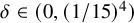 $\delta \in (0, (1/15)^4)$
. Consequently,
$\delta \in (0, (1/15)^4)$
. Consequently,
 $\mathbb {P}(Y_{\text {max}}=\infty )>3/4.$
Finally, recalling
$\mathbb {P}(Y_{\text {max}}=\infty )>3/4.$
Finally, recalling
 $\mathcal {I}_1$
from (133),
$\mathcal {I}_1$
from (133),
 $\mathbb {P}(\mathcal {I}_1)>1/3$
for large enough K by Claim 6.6. By the stochastic dominance in (134), it follows from a union bound that
$\mathbb {P}(\mathcal {I}_1)>1/3$
for large enough K by Claim 6.6. By the stochastic dominance in (134), it follows from a union bound that
This proves local survival of ![]() with positive probability.
with positive probability.
Proof of Theorem 2.1.
Lemma 6.4 states that for some
 $M\ge 1$
there exists
$M\ge 1$
there exists
 $K_1$
such that for
$K_1$
such that for
 $K>K_1$
and
$K>K_1$
and
 $\ell (K)$
as in (109)
$\ell (K)$
as in (109)
 $H_{K,\ell (K)}$
can be M-embedded in
$H_{K,\ell (K)}$
can be M-embedded in
 $\mathcal {T}$
almost surely. Set
$\mathcal {T}$
almost surely. Set
 $\bar \lambda =\lambda /M^{2\mu }$
and let
$\bar \lambda =\lambda /M^{2\mu }$
and let
 $K_0(\bar \lambda )$
be given by Lemma 6.8. Now let
$K_0(\bar \lambda )$
be given by Lemma 6.8. Now let
 $K>\max (K_0(\bar \lambda ),K_1)$
. Then Lemma 6.4 yields that
$K>\max (K_0(\bar \lambda ),K_1)$
. Then Lemma 6.4 yields that
 $H_{K,\ell (K)}$
can be M-embedded in
$H_{K,\ell (K)}$
can be M-embedded in
 $\mathcal {T}$
almost surely. Let
$\mathcal {T}$
almost surely. Let
 $v_1$
be the center of the first star in the embedded
$v_1$
be the center of the first star in the embedded
 $H_{K,\ell (K)}$
. Recalling (108) in Definition 6.3, we observe that the process
$H_{K,\ell (K)}$
. Recalling (108) in Definition 6.3, we observe that the process ![]() restricted to the vertices of the embedded
restricted to the vertices of the embedded
 $H_{K,\ell (K)}$
is stochastically dominated from below by the process
$H_{K,\ell (K)}$
is stochastically dominated from below by the process ![]() on a standalone copy of
on a standalone copy of
 $H_{K,\ell (K)}$
. Combining this with Lemma 6.8 and
$H_{K,\ell (K)}$
. Combining this with Lemma 6.8 and
 $K\ge K_0(\bar \lambda )$
implies that
$K\ge K_0(\bar \lambda )$
implies that ![]() survives locally with positive probability. This, along with the fact that with positive probability,
survives locally with positive probability. This, along with the fact that with positive probability, ![]() infects
infects
 $v_1$
at some point in time finishes the proof.
$v_1$
at some point in time finishes the proof.

7 The configuration model: k-cores sustain the infection when stars do not
In this section we will prove part (b) of Theorem 2.8. A crucial difference between the classical contact process and the degree-dependent version in this regime is that star-graphs do not sustain the infection, in fact they heal quickly when
 $\mu>1/2$
, by Claim 6.6. However, we know from Section 6.1 that the approximating Galton-Watson tree shows global survival (only), which suggests long survival on the configuration model. So we set out to find a new structure – a subgraph – embedded in the configuration model that sustains the degree-dependent contact process for a long time. Generally speaking, any (sparse) graph can sustain the infection linearly long in its number of edges (or vertices), hence to prove exponentially long survival in n we aim for this subgraph to have linearly many vertices in n.
$\mu>1/2$
, by Claim 6.6. However, we know from Section 6.1 that the approximating Galton-Watson tree shows global survival (only), which suggests long survival on the configuration model. So we set out to find a new structure – a subgraph – embedded in the configuration model that sustains the degree-dependent contact process for a long time. Generally speaking, any (sparse) graph can sustain the infection linearly long in its number of edges (or vertices), hence to prove exponentially long survival in n we aim for this subgraph to have linearly many vertices in n.
To find such a subgraph, we need to take into account that vertices that have either too high or too low degree cannot sustain the infection, either because the penalty f on them is too high or because
 $\lambda $
is assumed to be close to
$\lambda $
is assumed to be close to
 $0$
. The subgraph we found is the k-core – a maximal subgraph of the configuration model where each vertex has degree at least k inside the same subgraph – but with a twist: in the original configuration model with fat-tailed degrees, the k-core contains vertices of very high degree (e.g., polynomials of n). However, the degree-dependent CP near these vertices would have too high penalty f, so we need to exclude them from the k-core.
$0$
. The subgraph we found is the k-core – a maximal subgraph of the configuration model where each vertex has degree at least k inside the same subgraph – but with a twist: in the original configuration model with fat-tailed degrees, the k-core contains vertices of very high degree (e.g., polynomials of n). However, the degree-dependent CP near these vertices would have too high penalty f, so we need to exclude them from the k-core.
As a result we look at the k-core of not the original configuration model, but the subgraph obtained after removing all vertices of degree above a threshold value M, where now M is a constant depending only on k but not on the total number of vertices n. It is a priori unclear whether such a low truncation value even produces a connected graph, let alone contains a linear-sized k-core (i.e., containing at least some constant times n vertices). So our first step is to study the dependence between
 $M=M(k)$
and k so that a linear sized k-core still exists in the configuration model where all vertices of degree above M are removed. As we will see, the exact relation between k and
$M=M(k)$
and k so that a linear sized k-core still exists in the configuration model where all vertices of degree above M are removed. As we will see, the exact relation between k and
 $M(k)$
will be crucial on whether the infection manages to spread: indeed, any vertex in the k-core can spread to (typically) k vertices while it (typically) experiences rate
$M(k)$
will be crucial on whether the infection manages to spread: indeed, any vertex in the k-core can spread to (typically) k vertices while it (typically) experiences rate
 $\lambda M(k)^{-\mu }$
coming from the original degrees. Intuitively, CP will survive on the k-core if
$\lambda M(k)^{-\mu }$
coming from the original degrees. Intuitively, CP will survive on the k-core if
 $k M(k)^{-\mu }$
is growing with k, which limits the value of
$k M(k)^{-\mu }$
is growing with k, which limits the value of
 $M(k)$
to a polynomial of k. We will show that “essentially the lowest” power of k we can achieve so that a linear k-core exists is
$M(k)$
to a polynomial of k. We will show that “essentially the lowest” power of k we can achieve so that a linear k-core exists is
 $M(k)=k^{(1+o(1))/(3-\tau )}$
, which then readily yields the
$M(k)=k^{(1+o(1))/(3-\tau )}$
, which then readily yields the
 $\mu <3-\tau -o(1)$
criterion for survival in Theorem 2.8.
$\mu <3-\tau -o(1)$
criterion for survival in Theorem 2.8.
After finding the linear-sized k-core on vertices of degree at most
 $M(k)$
, we show that
$M(k)$
, we show that
 ${\mathrm {CP}}_{f,\lambda }$
survives on this k-core. For this step, our proof is a nontrivial adaptation of the proof of [Reference Mourrat and Valesin56, Theorem 1.2(b)], which shows long survival in the original contact process model on
${\mathrm {CP}}_{f,\lambda }$
survives on this k-core. For this step, our proof is a nontrivial adaptation of the proof of [Reference Mourrat and Valesin56, Theorem 1.2(b)], which shows long survival in the original contact process model on
 $(d+1)$
-regular random graphs, when
$(d+1)$
-regular random graphs, when
 $\lambda $
is above the lower critical
$\lambda $
is above the lower critical
 $\lambda _1(\mathbb {T}^d)$
on d-regular trees needed for global survival [Reference Pemantle57]. However, in our case we have
$\lambda _1(\mathbb {T}^d)$
on d-regular trees needed for global survival [Reference Pemantle57]. However, in our case we have
 $\lambda $
arbitrarily close to
$\lambda $
arbitrarily close to
 $0$
. Fortunately, we can choose k as a function of
$0$
. Fortunately, we can choose k as a function of
 $\lambda $
that makes the process locally supercritical. This also makes the proof different from that in [Reference Mourrat and Valesin56] even beyond finding the k-cores. First, we define the k-core of a graph.
$\lambda $
that makes the process locally supercritical. This also makes the proof different from that in [Reference Mourrat and Valesin56] even beyond finding the k-cores. First, we define the k-core of a graph.
Definition 7.1. Let G be any simple, finite graph. For a fixed positive integer k, the k-core of G is the largest induced subgraph
 $\mathrm {Core}_k(G)$
of G such that every vertex in
$\mathrm {Core}_k(G)$
of G such that every vertex in
 $\mathrm {Core}_k(G)$
has degree at least k within
$\mathrm {Core}_k(G)$
has degree at least k within
 $\mathrm {Core}_k(G)$
.
$\mathrm {Core}_k(G)$
.
It is not hard to see that the k-core
 $\mathrm {Core}_k(G)$
in Definition 7.1 is well-defined – but may be empty – by the following algorithm producing it. First, delete all vertices of G that have degree less than k along with their incident edges. Then do the same with the resulting graph, repeatedly, until no new vertex is deleted. The output of this algorithm is the unique largest induced subgraph of G with all degrees at least k. Note that the k-core of a graph might be empty or may contain more than one component.
$\mathrm {Core}_k(G)$
in Definition 7.1 is well-defined – but may be empty – by the following algorithm producing it. First, delete all vertices of G that have degree less than k along with their incident edges. Then do the same with the resulting graph, repeatedly, until no new vertex is deleted. The output of this algorithm is the unique largest induced subgraph of G with all degrees at least k. Note that the k-core of a graph might be empty or may contain more than one component.
7.1 The subgraph spanned on low-degree vertices contains a k-core
Our first goal is to prove the existence of a k-core in the configuration model after we remove all vertices with too high degrees. Throughout this section, we work with the configuration model
 $\mathrm {CM}(\underline d_n)=:G$
in Definition 1.9 on the degree sequence
$\mathrm {CM}(\underline d_n)=:G$
in Definition 1.9 on the degree sequence
 $\underline d_n=(d_1, \dots , d_n)$
that satisfies the regularity assumptions in Assumption 1.10, and the weak power-law empirical degrees of Assumption 1.11 with exponent
$\underline d_n=(d_1, \dots , d_n)$
that satisfies the regularity assumptions in Assumption 1.10, and the weak power-law empirical degrees of Assumption 1.11 with exponent
 $\tau>2$
and error
$\tau>2$
and error
 $\varepsilon>0$
.
$\varepsilon>0$
.
We now set up the procedure of removing all vertices above some degree M and the edges attached to those in
 $\mathrm {CM}(\underline d_n)$
. This is often called a targeted attack on the graph. Because the graph is formed by a random matching, and the half-edges that have one endpoint at a vertex with degree larger than M and another endpoint at a vertex with degree at most M are also removed, the degrees in the remaining graph are random.
$\mathrm {CM}(\underline d_n)$
. This is often called a targeted attack on the graph. Because the graph is formed by a random matching, and the half-edges that have one endpoint at a vertex with degree larger than M and another endpoint at a vertex with degree at most M are also removed, the degrees in the remaining graph are random.
Definition 7.2 (Configuration model under targeted attack).
Consider the configuration model
 $\mathrm {CM}(\underline d_n)$
in Definition 1.9 on the degree sequence
$\mathrm {CM}(\underline d_n)$
in Definition 1.9 on the degree sequence
 $\underline d_n=(d_1, \dots , d_n)$
. Fix some value
$\underline d_n=(d_1, \dots , d_n)$
. Fix some value
 $M\ge 0$
. Denote
$M\ge 0$
. Denote

Let
 $G_n[\mathcal {V}_{\le M}]$
denote the (random) subgraph of
$G_n[\mathcal {V}_{\le M}]$
denote the (random) subgraph of
 $\mathrm {CM}(\underline d_n)$
that is spanned on the vertex set
$\mathrm {CM}(\underline d_n)$
that is spanned on the vertex set
 $\mathcal {V}_{\le M}$
. For any
$\mathcal {V}_{\le M}$
. For any
 $v\in \mathcal {V}_{\le M}$
, we denote the random degree of v in
$v\in \mathcal {V}_{\le M}$
, we denote the random degree of v in
 $G_n[\mathcal {V}_{\le M}]$
by
$G_n[\mathcal {V}_{\le M}]$
by
 $\widetilde d_v$
, and we write
$\widetilde d_v$
, and we write
 $\widetilde n_i$
for the number of vertices with degree i in
$\widetilde n_i$
for the number of vertices with degree i in
 $G_n[\mathcal {V}_{\le M}]$
. For any
$G_n[\mathcal {V}_{\le M}]$
. For any
 $z\ge 0$
define
$z\ge 0$
define

and let
 $\widetilde D_{n,M}$
denote a random variable with cdf
$\widetilde D_{n,M}$
denote a random variable with cdf
 $\widetilde F_{n,M}(z)$
.
$\widetilde F_{n,M}(z)$
.
Observe that
 $\widetilde F_{n,M}(z)$
is the new empirical distribution of the degrees, after the targeted attack. This distribution is random, caused by the random matching that generated the graph before the attack. The quantities in (141) all depend on n, which we suppress in notation. We are ready to state the existence of the k-core in the configuration model under attack.
$\widetilde F_{n,M}(z)$
is the new empirical distribution of the degrees, after the targeted attack. This distribution is random, caused by the random matching that generated the graph before the attack. The quantities in (141) all depend on n, which we suppress in notation. We are ready to state the existence of the k-core in the configuration model under attack.
Theorem 7.3. Consider the configuration model
 $\mathrm {CM}(\underline d_n)=:G_n$
in Definition 1.9 on the degree sequence
$\mathrm {CM}(\underline d_n)=:G_n$
in Definition 1.9 on the degree sequence
 $\underline d_n=(d_1, \dots , d_n)$
that satisfies the regularity assumptions in Assumption 1.10, and the weak power-law empirical degrees of Assumption 1.11 with exponent
$\underline d_n=(d_1, \dots , d_n)$
that satisfies the regularity assumptions in Assumption 1.10, and the weak power-law empirical degrees of Assumption 1.11 with exponent
 $\tau \in (2,3)$
and error
$\tau \in (2,3)$
and error
 $\varepsilon>0$
. Let
$\varepsilon>0$
. Let
 $$ \begin{align} \eta_{\min}:=\frac{(3-\tau)}{(3-\tau)-\varepsilon(\tau-1)}\cdot \frac{1+\varepsilon}{1-\varepsilon}-1, \end{align} $$
and assume
 $\tau , \varepsilon $
are such that
$\tau , \varepsilon $
are such that
 $\eta _{\min }\in [0,\infty )$
. Fix a large enough positive integer k, and for any
$\eta _{\min }\in [0,\infty )$
. Fix a large enough positive integer k, and for any
 $\eta>\eta _{\min }$
let
$\eta>\eta _{\min }$
let
 $M:=M_{k,\eta }=k^{(1+\eta )/(3-\tau )}$
. Let
$M:=M_{k,\eta }=k^{(1+\eta )/(3-\tau )}$
. Let
 $G_n[\mathcal {V}_{\le M}]$
be the configuration model under attack in Definition 7.2, and denote by
$G_n[\mathcal {V}_{\le M}]$
be the configuration model under attack in Definition 7.2, and denote by
 $\mathrm {Core}_{k}(G_n[\mathcal {V}_{\le M}])$
its k-core. Then there exists some
$\mathrm {Core}_{k}(G_n[\mathcal {V}_{\le M}])$
its k-core. Then there exists some
 $\rho =\rho (k)>0$
such that
$\rho =\rho (k)>0$
such that
 $$ \begin{align} \lim_{n\to \infty} \mathbb{P} \Big( |\mathrm{Core}_{k}(G_n[\mathcal{V}_{\le M}])| \ge \rho n \Big) =1, \end{align} $$
Further, conditioned on its vertex set and degree sequence,
 $\mathrm {Core}_{k}(G_n[\mathcal {V}_{\le M}])$
is itself a configuration model.
$\mathrm {Core}_{k}(G_n[\mathcal {V}_{\le M}])$
is itself a configuration model.
Remark 7.4 (Asymptotics of
$\rho $
).

The proof of Theorem 7.3 shows that there exists a constant
 $c'>0$
such that
$c'>0$
such that
 $$ \begin{align} \rho(k)> c' k^{-\tfrac{(\tau-1)(1+\varepsilon)}{(2-(\tau-1)(1+\varepsilon))}}. \end{align} $$
Note that in this lower estimate only the lower bound exponent in Assumption 1.11 appears. We comment that
 $\eta _{\min }\in [0, \infty )$
implies that
$\eta _{\min }\in [0, \infty )$
implies that
 $\varepsilon <(3-\tau )/(\tau -1)$
, which is exactly the condition that the lower bound on the tail-exponent,
$\varepsilon <(3-\tau )/(\tau -1)$
, which is exactly the condition that the lower bound on the tail-exponent,
 $(\tau -1)(1+\varepsilon )$
in (9), stays strictly below
$(\tau -1)(1+\varepsilon )$
in (9), stays strictly below
 $2$
. Hence a k-core exists for all k when the estimates on the empirical power law are so that the tail is always heavier than a power law with infinite variance. Without the truncation at M, that is, for pure power laws, such a result is already known, see [Reference Janson and Luczak37] and [Reference Fernholz and Ramachandran28]. Here we specify the truncation value M for which the result stays valid. We comment that when
$2$
. Hence a k-core exists for all k when the estimates on the empirical power law are so that the tail is always heavier than a power law with infinite variance. Without the truncation at M, that is, for pure power laws, such a result is already known, see [Reference Janson and Luczak37] and [Reference Fernholz and Ramachandran28]. Here we specify the truncation value M for which the result stays valid. We comment that when
 $\varepsilon =0$
in Assumption 1.11, then our proof can be strengthened so that
$\varepsilon =0$
in Assumption 1.11, then our proof can be strengthened so that
 $M=\Theta (k^{1/(3-\tau )})$
guarantees the existence of a large k-core after the targeted attack.
$M=\Theta (k^{1/(3-\tau )})$
guarantees the existence of a large k-core after the targeted attack.
We will prove Theorem 7.3 below using the following two lemmas and the results of Janson and Luczak [Reference Janson and Luczak37] that we will state soon. The first lemma says that the random empirical distribution of
 $G_n[\mathcal {V}_{\le M}]$
converges in probability, assuming the regularity assumptions on the original degrees. We use notation from Definition 7.2. Given the degree sequence
$G_n[\mathcal {V}_{\le M}]$
converges in probability, assuming the regularity assumptions on the original degrees. We use notation from Definition 7.2. Given the degree sequence
 $\underline d_n$
,
$\underline d_n$
,
 $D_n$
stands for the random variable that follows the empirical distribution
$D_n$
stands for the random variable that follows the empirical distribution
 $F_n$
of
$F_n$
of
 $\underline d_n$
in (8), and D is the random variable following the limiting distribution in Assumption 1.10. Define then
$\underline d_n$
in (8), and D is the random variable following the limiting distribution in Assumption 1.10. Define then
and we collect the errors below M between the n-dependent degree distribution
 $D_n$
and the limit D as follows:
$D_n$
and the limit D as follows:
 $$ \begin{align} \begin{aligned} \delta_n:=\max\Big\{&|q_{n,M}/q_M-1|,\ |(1-q_{n,M})/(1-q_M)-1|, \\ &\ \max_{i\le M, \mathbb{P}(D=i)=0 } \mathbb{P}(D_n=i), \max_{i\le M, \mathbb{P}(D=i)\neq 0}|\mathbb{P}(D_n=i)/\mathbb{P}(D=i)-1|\Big\}, \end{aligned} \end{align} $$
with
 $\delta _n\to 0$
when Assumption 1.10 holds. Typically, for M large
$\delta _n\to 0$
when Assumption 1.10 holds. Typically, for M large
 $q_M$
is close to
$q_M$
is close to
 $1$
so the relative error of
$1$
so the relative error of
 $1-q_{M,n}$
to
$1-q_{M,n}$
to
 $1-q_M$
is driving the maximum in the first row, while the second row is only over values
$1-q_M$
is driving the maximum in the first row, while the second row is only over values
 $i\le M$
.
$i\le M$
.
Lemma 7.5 (Degree distribution of CM under attack).
Consider the configuration model
 $\mathrm {CM}(\underline d_n)$
in Definition 1.9 on the degree sequence
$\mathrm {CM}(\underline d_n)$
in Definition 1.9 on the degree sequence
 $\underline d_n=(d_1, \dots , d_n)$
that satisfies the regularity assumptions in Assumption 1.10. Fix any
$\underline d_n=(d_1, \dots , d_n)$
that satisfies the regularity assumptions in Assumption 1.10. Fix any
 $M>0$
constant, and let
$M>0$
constant, and let
 $q_{n,M}, q_M, \delta _n$
as in (146) and (147). Define the following random variable
$q_{n,M}, q_M, \delta _n$
as in (146) and (147). Define the following random variable
 $\widetilde D_M$
: for all
$\widetilde D_M$
: for all
 $i\le M$
, let
$i\le M$
, let
 $$ \begin{align} \begin{aligned} p_{M}(i)&:=\mathbb{P}(\widetilde D_M=i) =\sum_{j=i}^M \frac{\mathbb{P}(D=j)}{\mathbb{P}(D\le M)} \binom{j}{i}q_M^i(1-q_M)^{j-i}\\ &= \mathbb{P}( \mathrm{Bin}(D, q_M)=i \mid D\le M). \end{aligned} \end{align} $$
Let
 $X_{n,M}(i):=\widetilde n_i/V_{\le M}=\mathbb {P}(\widetilde D_{n,M}=i\mid G_n[\mathcal {V}_{\le M}])$
be the random empirical degree distribution of
$X_{n,M}(i):=\widetilde n_i/V_{\le M}=\mathbb {P}(\widetilde D_{n,M}=i\mid G_n[\mathcal {V}_{\le M}])$
be the random empirical degree distribution of
 $G_n[\mathcal {V}_{\le M}]$
. Then for all
$G_n[\mathcal {V}_{\le M}]$
. Then for all
 $\varepsilon _n>0$
that satisfies
$\varepsilon _n>0$
that satisfies
 $\varepsilon _n \gg \max \{\delta _n, 1/\sqrt {n}\}$
,
$\varepsilon _n \gg \max \{\delta _n, 1/\sqrt {n}\}$
,
 $$ \begin{align} \mathbb{P}\Big(\sup_{i\le M}\big| X_{n,M}(i)-p_M(i)\big| \ge \varepsilon_n \Big) = O\bigg(\frac{M^3}{n\varepsilon^{2}_n}\bigg)\to 0. \end{align} $$
Further,
 $\lim _{n\to \infty }\mathbb {E}[\widetilde D_{n,M}\mid G_n[\mathcal {V}_{\le M}]]=\mathbb {E}[\widetilde D_M]$
in probability. So, the empirical degree distribution
$\lim _{n\to \infty }\mathbb {E}[\widetilde D_{n,M}\mid G_n[\mathcal {V}_{\le M}]]=\mathbb {E}[\widetilde D_M]$
in probability. So, the empirical degree distribution
 $\widetilde D_{n,M}$
of
$\widetilde D_{n,M}$
of
 $G_n[\mathcal {V}_{\le M}]$
satisfies Assumption 1.10 with probability tending to
$G_n[\mathcal {V}_{\le M}]$
satisfies Assumption 1.10 with probability tending to
 $1$
. Furthermore,
$1$
. Furthermore,
 $G_n[\mathcal {V}_{\le M}]$
is itself a configuration model on its vertex set, conditioned on the degrees of its vertices.
$G_n[\mathcal {V}_{\le M}]$
is itself a configuration model on its vertex set, conditioned on the degrees of its vertices.
The second lemma proves that the limiting degree distribution of
 $G_n[\mathcal {V}_{\le M}]$
is a truncated weak power law with truncation close to M if the original degree distribution satisfied the weak power law assumption.
$G_n[\mathcal {V}_{\le M}]$
is a truncated weak power law with truncation close to M if the original degree distribution satisfied the weak power law assumption.
Lemma 7.6 (Truncated power laws after targeted attack).
Consider the configuration model
 $\mathrm {CM}(\underline d_n)$
in Definition 1.9 on the degree sequence
$\mathrm {CM}(\underline d_n)$
in Definition 1.9 on the degree sequence
 $\underline d_n=(d_1, \dots , d_n)$
that satisfies the regularity assumptions in Assumption 1.10, and the power-law empirical degrees of Assumption 1.11 with exponent
$\underline d_n=(d_1, \dots , d_n)$
that satisfies the regularity assumptions in Assumption 1.10, and the power-law empirical degrees of Assumption 1.11 with exponent
 $\tau $
and exponent-error
$\tau $
and exponent-error
 $\varepsilon \ge 0$
. Let
$\varepsilon \ge 0$
. Let
 $M>0$
be a constant (i.e., not depending on n, but it may depend on
$M>0$
be a constant (i.e., not depending on n, but it may depend on
 $\varepsilon $
), and let
$\varepsilon $
), and let
 $$ \begin{align} \widetilde z_{\max}(M):=2^{-1}(c_\ell/(2c_u))^{\tfrac{1}{(\tau-1)(1+\varepsilon)}} M^{(1-\varepsilon)/(1+\varepsilon)}. \end{align} $$
Consider the limiting degree distribution
 $\widetilde F_M(z)=:\sum _{i\le z} p_M(i)$
in (148) of
$\widetilde F_M(z)=:\sum _{i\le z} p_M(i)$
in (148) of
 $G_n[\mathcal {V}_{\le M}]$
in Lemma 7.5. Then there exist constants
$G_n[\mathcal {V}_{\le M}]$
in Lemma 7.5. Then there exist constants
 $\widetilde c_\ell , \widetilde c_u, M_0$
, such that whenever
$\widetilde c_\ell , \widetilde c_u, M_0$
, such that whenever
 $M\ge M_0$
, for all
$M\ge M_0$
, for all
 $z\in [z_0, \widetilde z_{\max }(M)]$
, it holds that
$z\in [z_0, \widetilde z_{\max }(M)]$
, it holds that
 $$ \begin{align} \frac{\widetilde c_\ell}{z^{(\tau-1)(1+\varepsilon)}} \le 1-\widetilde F_{M}(z) \le \frac{\widetilde c_u}{z^{(\tau-1)(1-\varepsilon)}}. \end{align} $$
The proof shows that
 $\widetilde c_\ell = c_\ell 2^{-(\tau -1)(1+\varepsilon )-2}$
and
$\widetilde c_\ell = c_\ell 2^{-(\tau -1)(1+\varepsilon )-2}$
and
 $\widetilde c_u=2c_u$
are valid choices (although they may not be optimal). Since the proofs of Lemmas 7.5 and 7.6 are fairly standard, we provide them in the Appendix on pages 78 and 82.
$\widetilde c_u=2c_u$
are valid choices (although they may not be optimal). Since the proofs of Lemmas 7.5 and 7.6 are fairly standard, we provide them in the Appendix on pages 78 and 82.
With these lemmas at hand, the proof of Theorem 7.3 relies on the result of Janson and Luczak [Reference Janson and Luczak37], describing the k-core of the configuration model. To state this result, we introduce some notation.
For a random variable D and
 $p\in [0,1]$
, we let
$p\in [0,1]$
, we let
 $X_{D,p}$
denote a random variable with Binomial(
$X_{D,p}$
denote a random variable with Binomial(
 $D,p$
) distribution. That is,
$D,p$
) distribution. That is,
 $$\begin{align*}\mathbb{P}(X_{D,p}=r)=\sum_{l=r}^\infty \mathbb{P}(D=l)\binom{l}{r}p^r(1-p)^{l-r}.\end{align*}$$
We then define the following functions:
Note that both h and
 $h_1$
are increasing in p, and
$h_1$
are increasing in p, and
 $h(D,0)=h_1(D,0)=0$
. Moreover,
$h(D,0)=h_1(D,0)=0$
. Moreover, ![]() , and
, and
 $h_1(D,1)=\mathbb {P}(D\ge k)\le 1$
.
$h_1(D,1)=\mathbb {P}(D\ge k)\le 1$
.
Then the theorem of Janson and Luczak is as follows. They use the same regularity Assumption 1.10 as we do.
Theorem 7.7 (Theorem 2.3 in [Reference Janson and Luczak37]).
Consider the configuration model
 $G_n:=\mathrm {CM}(\underline d_n)$
in Definition 1.9 on the degree sequence
$G_n:=\mathrm {CM}(\underline d_n)$
in Definition 1.9 on the degree sequence
 $\underline d_n=(d_1, \dots , d_n)$
that satisfies the regularity assumptions in Assumption 1.10. For
$\underline d_n=(d_1, \dots , d_n)$
that satisfies the regularity assumptions in Assumption 1.10. For
 $k\ge 2$
be fixed, let
$k\ge 2$
be fixed, let
 $\mathrm {Core}_k:=\mathrm {Core}_k(G_n)$
be the k-core of
$\mathrm {Core}_k:=\mathrm {Core}_k(G_n)$
be the k-core of
 $G_n$
. Let
$G_n$
. Let
 $$ \begin{align} \hat p:= \max\{ p\le 1: \mathbb{E}[D] p^2=h(D,p) \}.\end{align} $$
Then, if
 $\hat {p}>0$
and
$\hat {p}>0$
and
 $\mathbb {E}[D] p^2<h(D,p)$
for p in some interval
$\mathbb {E}[D] p^2<h(D,p)$
for p in some interval
 $(\hat {p}-\varepsilon ,\hat {p})$
, then
$(\hat {p}-\varepsilon ,\hat {p})$
, then
 $\mathrm {Core}_k(G_n)$
is nonempty whp, and
$\mathrm {Core}_k(G_n)$
is nonempty whp, and
 $$ \begin{align} |\mathcal{V}(\mathrm{Core}_k)|/n\ {\buildrel \mathbb P \over \longrightarrow}\ h_1(D,\hat{p}), \qquad |\mathcal{E}(\mathrm{Core}_k)|/n {\buildrel \mathbb P \over \longrightarrow}\ h(D,\hat{p})/2=\mathbb{E}[D] \hat{p}^2/2. \end{align} $$
We first need a small extension of this theorem.
Claim 7.8. Suppose there is a value
 $p_-$
where
$p_-$
where
 $\mathbb {E}[D]p_-^2<h(D,p_-)$
holds (see below (153)). Then, there is a nonzero fixed point
$\mathbb {E}[D]p_-^2<h(D,p_-)$
holds (see below (153)). Then, there is a nonzero fixed point
 $p_\star>p_-$
of (153) so that in the interval
$p_\star>p_-$
of (153) so that in the interval
 $(p_\star , p_\star -\varepsilon )$
the inequality
$(p_\star , p_\star -\varepsilon )$
the inequality
 $\mathbb {E}[D]p^2<h(D,p)$
holds. Then,
$\mathbb {E}[D]p^2<h(D,p)$
holds. Then,
 $\mathrm {Core_k}(G_n)$
is nonempty and
$\mathrm {Core_k}(G_n)$
is nonempty and
 $$ \begin{align} \begin{aligned} \mathbb{P}&\Big(|\mathcal{V}(\mathrm{Core_k})|/n \le h_1(D, p_-) (1-\varepsilon)\Big)\\ &\le \mathbb{P}\Big(|\mathcal{V}(\mathrm{Core_k})|/n \le h_1(D, p_\star) (1-\varepsilon)\Big) \to 0 \end{aligned} \end{align} $$
as
 $n\to \infty $
.
$n\to \infty $
.
Sketch of proof.
The first statement, namely that
 $p^\star $
exists, follows from the continuity of the function
$p^\star $
exists, follows from the continuity of the function
 $\mathbb {E}[D]p^2-h(D,p)$
. The second statement, that the size of the k-core is at least
$\mathbb {E}[D]p^2-h(D,p)$
. The second statement, that the size of the k-core is at least
 $h_1(D, p_\star )(1-\varepsilon )$
, follows from the proof of [Reference Janson and Luczak37, Theorem 2.3]. Namely, the only case where the proof of [Reference Janson and Luczak37, Theorem 2.3] does not apply directly is where the function
$h_1(D, p_\star )(1-\varepsilon )$
, follows from the proof of [Reference Janson and Luczak37, Theorem 2.3]. Namely, the only case where the proof of [Reference Janson and Luczak37, Theorem 2.3] does not apply directly is where the function
 $f(p)=E[D]p^2-h(D,p)$
does not cross the
$f(p)=E[D]p^2-h(D,p)$
does not cross the
 $0$
-line at its maximal
$0$
-line at its maximal
 $0$
but rather, it touches it. Nevertheless, if one finds a smaller value
$0$
but rather, it touches it. Nevertheless, if one finds a smaller value
 $p_-$
where the function
$p_-$
where the function
 $f(p)$
is in the negative, it implies that there must be zero-point
$f(p)$
is in the negative, it implies that there must be zero-point
 $p_\star $
of f where the function crosses the
$p_\star $
of f where the function crosses the
 $0$
level line. In this case the proof there yields that the density of the k-core is at least
$0$
level line. In this case the proof there yields that the density of the k-core is at least
 $h_1(D, p_\star )$
, hence (155) holds. This can be found on [Reference Janson and Luczak37, page 56-57], where a value
$h_1(D, p_\star )$
, hence (155) holds. This can be found on [Reference Janson and Luczak37, page 56-57], where a value
 $p_-$
for which
$p_-$
for which
 $f(p_-)<0$
implies the upper bound on the stopping time of a pruning algorithm generating the k-core for (154). That is, the continuous time pruning algorithm of sequentially removing vertices of degrees at least k and their outgoing edges is guaranteed to stop by time
$f(p_-)<0$
implies the upper bound on the stopping time of a pruning algorithm generating the k-core for (154). That is, the continuous time pruning algorithm of sequentially removing vertices of degrees at least k and their outgoing edges is guaranteed to stop by time
 $t=-\log (p_-)$
, that is, one can set
$t=-\log (p_-)$
, that is, one can set
 $t_2=-\log (p_-)$
at the bottom [Reference Janson and Luczak37, page 9]. An upper bound on the stopping of the pruning algorithm gives a lower bound on the number of remaining vertices forming the k-core. In our case, by not knowing whether
$t_2=-\log (p_-)$
at the bottom [Reference Janson and Luczak37, page 9]. An upper bound on the stopping of the pruning algorithm gives a lower bound on the number of remaining vertices forming the k-core. In our case, by not knowing whether
 $p_-$
is adjacent to the maximal fixed point and whether f touches or crosses
$p_-$
is adjacent to the maximal fixed point and whether f touches or crosses
 $0$
there, we lose the upper bound on the k-core size.
$0$
there, we lose the upper bound on the k-core size.
With Lemmas 7.5 and 7.6 at hand, we are ready to prove Theorem 7.3 by checking the conditions of Theorem 7.7 and Claim 7.8.
Proof of Theorem 7.3.
First, we prove (144) holds: we will check that the conditions of Theorem 7.7 hold for
 $G_n[\mathcal {V}_{\le M}]$
with probability tending to
$G_n[\mathcal {V}_{\le M}]$
with probability tending to
 $1$
. First, Lemma 7.5 implies that
$1$
. First, Lemma 7.5 implies that
 $G_n[\mathcal {V}_{\le M}]$
is a configuration model (conditioned on its vertices and their degrees), and its (random) degree sequence satisfies Assumption 1.10 with probability tending to
$G_n[\mathcal {V}_{\le M}]$
is a configuration model (conditioned on its vertices and their degrees), and its (random) degree sequence satisfies Assumption 1.10 with probability tending to
 $1$
. We will use the notations of Lemmas 7.5 – 7.6, so,
$1$
. We will use the notations of Lemmas 7.5 – 7.6, so,
 $\widetilde D_M$
denotes the limiting degree distribution of
$\widetilde D_M$
denotes the limiting degree distribution of
 $G_n[\mathcal {V}_{\le M}]$
. Since
$G_n[\mathcal {V}_{\le M}]$
. Since
 $h(\widetilde D_M,p)$
in (152) is a continuous function of p, it is enough for us to find a particular choice of p with
$h(\widetilde D_M,p)$
in (152) is a continuous function of p, it is enough for us to find a particular choice of p with
 $\mathbb {E}[\widetilde D_M]p^2<h(\widetilde D_M,p)$
. Based on the tail probabilities of
$\mathbb {E}[\widetilde D_M]p^2<h(\widetilde D_M,p)$
. Based on the tail probabilities of
 $\widetilde D_M$
from (151), in particular the exponent
$\widetilde D_M$
from (151), in particular the exponent
 $\tau \in (2,3)$
and the constant
$\tau \in (2,3)$
and the constant
 $\widetilde c_\ell $
in the lower bound, which holds for
$\widetilde c_\ell $
in the lower bound, which holds for
 $z\in [z_0,\widetilde z_{\max }(M)]$
with
$z\in [z_0,\widetilde z_{\max }(M)]$
with
 $\widetilde z_{\max }(M)$
defined in (150), our goal is to find two positive constants
$\widetilde z_{\max }(M)$
defined in (150), our goal is to find two positive constants
 $a_-< a_+$
and
$a_-< a_+$
and
 $\xi>3-\tau $
and an interval
$\xi>3-\tau $
and an interval
 $$ \begin{align} I_p:=[p_-, p_+]:=\Big[ a_- k^{-(\xi/(3-\tau)-1)}, a_+ k^{-(\xi/(3-\tau)-1)}\Big]. \end{align} $$
We will show that when
 $p\in I_p$
, then
$p\in I_p$
, then
 $\mathbb {E}[\widetilde D_M]p^2<h(\widetilde D_M,p)$
. Using (152), and that
$\mathbb {E}[\widetilde D_M]p^2<h(\widetilde D_M,p)$
. Using (152), and that
 $X_{l_1, p}$
stochastically dominates
$X_{l_1, p}$
stochastically dominates
 $X_{l_2, p}$
when
$X_{l_2, p}$
when
 $l_2>l_1$
, we estimate, for some constant
$l_2>l_1$
, we estimate, for some constant
 $\beta $
and exponent
$\beta $
and exponent
 $\xi>3-\tau $
to be chosen later,
$\xi>3-\tau $
to be chosen later,

We bound the first factor on the rhs of (157) first. Recalling that the tail-bound on
 $\mathbb {P}(\widetilde D_M>z)$
in (151), we get
$\mathbb {P}(\widetilde D_M>z)$
in (151), we get
 $$ \begin{align} \mathbb{P}\big(\widetilde D_M\ge \beta k^{\xi/(3-\tau)}\big)\ge \widetilde c_\ell \left(\beta k^{\xi/(3-\tau)}\right)^{-(\tau-1)(1+\varepsilon)}, \end{align} $$
on the condition that
 $\beta k^{\xi /(3-\tau )}\le \widetilde z_{\mathrm {max}}(M)$
which we now check. (This is the place where we need that the truncation point M is high enough.) We expand
$\beta k^{\xi /(3-\tau )}\le \widetilde z_{\mathrm {max}}(M)$
which we now check. (This is the place where we need that the truncation point M is high enough.) We expand
 $\widetilde z_{\mathrm {max}}(M)$
in (150) as a function of k using that
$\widetilde z_{\mathrm {max}}(M)$
in (150) as a function of k using that
 $M=k^{(1+\eta )/(3-\tau )}$
below (143). We write
$M=k^{(1+\eta )/(3-\tau )}$
below (143). We write
 $\widetilde C$
for the prefactor in (150) that only depends on
$\widetilde C$
for the prefactor in (150) that only depends on
 $c_\ell , c_u, \tau ,\varepsilon $
:
$c_\ell , c_u, \tau ,\varepsilon $
:
 $$ \begin{align} \widetilde z_{\mathrm{max}}(M)=\widetilde C M^{(1-\varepsilon)/(1+\varepsilon)}=\widetilde C k^{\left(\frac{1+\eta}{3-\tau}\right)(1-\varepsilon)/(1+\varepsilon)}. \end{align} $$
Treating
 $\beta , \widetilde C$
as constants while k can be chosen arbitrarily large, the rhs of (159) is larger than
$\beta , \widetilde C$
as constants while k can be chosen arbitrarily large, the rhs of (159) is larger than
 $\beta k^{\xi /(3-\tau )}$
for all sufficiently large k when
$\beta k^{\xi /(3-\tau )}$
for all sufficiently large k when
 $$ \begin{align} \xi<(1+\eta)(1-\varepsilon)/(1+\varepsilon), \end{align} $$
which shall lead to the assumption that
 $\eta>\eta _{\min }$
in (143) shortly. Next, we bound the second factor on the rhs of (157). For any variable X, it holds that
$\eta>\eta _{\min }$
in (143) shortly. Next, we bound the second factor on the rhs of (157). For any variable X, it holds that ![]() . In (157)
. In (157)
 $X\sim \mathrm {Bin}( \beta k^{\xi /(3-\tau )},p)$
, and with the choice
$X\sim \mathrm {Bin}( \beta k^{\xi /(3-\tau )},p)$
, and with the choice
 $a_-:=2/\beta $
, we can lower bound its mean using that
$a_-:=2/\beta $
, we can lower bound its mean using that
 $p>p_-$
in (156) as
$p>p_-$
in (156) as
 $\beta k^{\xi /(3-\tau )}p>2k^{\xi /(3-\tau )}k^{-(\xi /(3-\tau )-1)}=2k$
. Hence, a Chernoff bound applies and we obtain that
$\beta k^{\xi /(3-\tau )}p>2k^{\xi /(3-\tau )}k^{-(\xi /(3-\tau )-1)}=2k$
. Hence, a Chernoff bound applies and we obtain that
 $$ \begin{align} k\mathbb{P}\big(X_{ \beta k^{\xi/(3-\tau)},p}<k\big)\le k\exp\left(-\beta k^{\xi/(3-\tau)}p/8\right)\le k\exp\left(-k/4\right), \end{align} $$
for all
 $p>p_-$
in (156). Using again that
$p>p_-$
in (156). Using again that
 $p>p_-$
implies
$p>p_-$
implies
 $\beta k^{\xi /(3-\tau )}p\ge 2k$
, the second factor in (157) can be bounded from below for all sufficiently large k as
$\beta k^{\xi /(3-\tau )}p\ge 2k$
, the second factor in (157) can be bounded from below for all sufficiently large k as
Substituting (158) and (162) into (157) gives, for all
 $\beta $
,
$\beta $
,
 $p>p_-$
in (156) and all
$p>p_-$
in (156) and all
 $\xi>3-\tau >0$
that
$\xi>3-\tau >0$
that
 $$ \begin{align} h(\widetilde D_M,p)\ge (\widetilde c_\ell/2)\cdot \beta^{1-(\tau-1)(1+\varepsilon)}k^{(1-(\tau-1)(1+\varepsilon))\xi/(3-\tau)}p. \end{align} $$
Thus,
 $h(\widetilde D_M,p)>\mathbb {E}[\widetilde D_M]p^2$
holds when
$h(\widetilde D_M,p)>\mathbb {E}[\widetilde D_M]p^2$
holds when
 $$ \begin{align} (\widetilde c_\ell/2) \beta^{1-(\tau-1)(1+\varepsilon)}k^{(1-(\tau-1)(1+\varepsilon))\xi/(3-\tau)}>\mathbb{E}[\widetilde D_M]p. \end{align} $$
At this point we still have the freedom of choosing
 $\beta $
and
$\beta $
and
 $\xi>3-\tau $
provided that the relation between
$\xi>3-\tau $
provided that the relation between
 $\eta ,\xi $
in (160) holds. Since
$\eta ,\xi $
in (160) holds. Since
 $p<a_+k^{-(\xi /(3-\tau )-1)}$
in (156), first we compare the powers of k on both sides. The inequality (164) holds for all sufficiently large k if
$p<a_+k^{-(\xi /(3-\tau )-1)}$
in (156), first we compare the powers of k on both sides. The inequality (164) holds for all sufficiently large k if
 $$\begin{align*}(1-(\tau-1)(1+\varepsilon))\xi/(3-\tau)\ge-(\xi/(3-\tau)-1). \end{align*}$$
After elementary computations, the smallest
 $\xi $
that satisfies this inequality, and hence the threshold
$\xi $
that satisfies this inequality, and hence the threshold
 $\eta $
for (160) is
$\eta $
for (160) is
 $$ \begin{align} \xi\ge \xi_{\min}:=\frac{3-\tau}{3-\tau-\varepsilon(\tau-1)}, \qquad \eta>\eta_{\min}= \frac{\xi_{\min}(1+\varepsilon)}{1-\varepsilon} -1, \end{align} $$
which equals
 $\eta _{\min }$
in (143). Comparing now constants on the two sides of (164) yields that
$\eta _{\min }$
in (143). Comparing now constants on the two sides of (164) yields that
 $$\begin{align*}a_+:=(\widetilde c_\ell/2\mathbb{E}[\widetilde D_M]) \beta^{1-(\tau-1)(1+\varepsilon)}.\end{align*}$$
Solving the inequality
 $a_-=2/\beta <a_+$
gives that the interval
$a_-=2/\beta <a_+$
gives that the interval
 $I_p$
is nonempty whenever
$I_p$
is nonempty whenever
 $$ \begin{align*} \beta>\left(4\mathbb{E}[\widetilde D_M]/\widetilde c_\ell\right)^{1/[2-(\tau-1)(1+\varepsilon)]}. \end{align*} $$
Summarizing, we have found that whenever
 $\beta $
satisfies this inequality, and p is in the interval
$\beta $
satisfies this inequality, and p is in the interval
 $$ \begin{align*} I_p=\Big[(2/\beta)\cdot k^{-(1/(3-\tau-\varepsilon(\tau-1)) -1)}, (\widetilde c_\ell/2\mathbb{E}[\widetilde D_M]) \beta^{1-(\tau-1)(1+\varepsilon)} k^{-(1/(3-\tau-\varepsilon(\tau-1)) -1)}\Big], \end{align*} $$
then the required inequality for the existence of the k-core holds. This implies that
 $\hat {p}>p_+$
, and we can estimate the asymptotic proportion of the k-core (154),
$\hat {p}>p_+$
, and we can estimate the asymptotic proportion of the k-core (154),
 $h_1(\widetilde D_M, \hat p)\ge h_1(\widetilde D_M, p_+)$
following similar steps as in (157):
$h_1(\widetilde D_M, \hat p)\ge h_1(\widetilde D_M, p_+)$
following similar steps as in (157):
 $$ \begin{align*} h_1(\widetilde D_M, \hat p) &\ge \mathbb{P}(\widetilde D_M\ge k^{\xi/(3-\tau)}) \mathbb{P}\big( X_{k^{\xi/(3-\tau)}, p_+}\ge k\big)\\ &\ge \widetilde c_\ell k^{-\xi(\tau-1)(1+\varepsilon)/(3-\tau)} (1-\exp(-k/4)), \end{align*} $$
using the same
 $\xi =\xi _{\min }$
and Chernoff bound as in (165) and in (161), yielding (145) in Remark 7.4.
$\xi =\xi _{\min }$
and Chernoff bound as in (165) and in (161), yielding (145) in Remark 7.4.
Finally, we need to check that conditioned on its vertex set and degree sequence,
 $\mathrm {Core}_{k}(G_n[\mathcal {V}_{\le M}])$
is itself a configuration model. This follows from the fact that every matching of half-edges within
$\mathrm {Core}_{k}(G_n[\mathcal {V}_{\le M}])$
is itself a configuration model. This follows from the fact that every matching of half-edges within
 $\mathrm {Core}_{k}(G_n[\mathcal {V}_{\le M}])$
, given its degree sequence, has equal probability by the construction of the configuration model.
$\mathrm {Core}_{k}(G_n[\mathcal {V}_{\le M}])$
, given its degree sequence, has equal probability by the construction of the configuration model.
This finishes the first combinatorial part, that is, the existence of a large k-core. We now (slowly) transition to studying the contact process on the k-core. The proof of Theorem 2.8(b) is based on a structural property of
 $\mathrm {Core}_{k}(G_n[\mathcal {V}_{\le M}])$
that we define next. This structural property guarantees that an infected set of vertices can pass the infection to many other vertices in a unit time step.
$\mathrm {Core}_{k}(G_n[\mathcal {V}_{\le M}])$
that we define next. This structural property guarantees that an infected set of vertices can pass the infection to many other vertices in a unit time step.
Definition 7.9 (
$(\delta ,k)$
-expansion).

Fix any
 $\delta \in (0,1)$
and an even positive integer k. We say that a (multi)graph G on n vertices is
$\delta \in (0,1)$
and an even positive integer k. We say that a (multi)graph G on n vertices is
 $(\delta ,k)$
-good if for every set
$(\delta ,k)$
-good if for every set
 $\{v_1,\ldots ,v_{\lfloor \delta n\rfloor }\}$
of
$\{v_1,\ldots ,v_{\lfloor \delta n\rfloor }\}$
of
 $\lfloor \delta n\rfloor $
vertices in G, we can choose a subset
$\lfloor \delta n\rfloor $
vertices in G, we can choose a subset
 $\mathcal {I}_g$
of the indices of size
$\mathcal {I}_g$
of the indices of size
 $|\mathcal {I}_g|\ge \lfloor \delta n\rfloor /8$
such that each
$|\mathcal {I}_g|\ge \lfloor \delta n\rfloor /8$
such that each
 $v_i: i\in \mathcal {I}_g$
has
$v_i: i\in \mathcal {I}_g$
has
 $k/2$
neighbors
$k/2$
neighbors
 $w_{i,1},\ldots ,w_{i,k/2}$
in G such that the vertices
$w_{i,1},\ldots ,w_{i,k/2}$
in G such that the vertices
 $v_i, i\in \mathcal {I}_g$
and
$v_i, i\in \mathcal {I}_g$
and
 $w_{i,j}, i\in \mathcal {I}_g, j\le k/2$
are all distinct.
$w_{i,j}, i\in \mathcal {I}_g, j\le k/2$
are all distinct.
A graph being
 $(\delta ,k)$
-good is somewhat stronger than requiring that the
$(\delta ,k)$
-good is somewhat stronger than requiring that the
 $1$
-neighborhood of any
$1$
-neighborhood of any
 $\lfloor \delta n\rfloor $
many vertices expands by a factor
$\lfloor \delta n\rfloor $
many vertices expands by a factor
 $k/16$
, since we need enough individual vertices that expand to
$k/16$
, since we need enough individual vertices that expand to
 $k/2$
different vertices. The following lemma proves that
$k/2$
different vertices. The following lemma proves that
 $\mathrm {Core}_{k}(G_n[\mathcal {V}_{\le M}])$
has the
$\mathrm {Core}_{k}(G_n[\mathcal {V}_{\le M}])$
has the
 $(\delta ,k)$
-good property for small enough
$(\delta ,k)$
-good property for small enough
 $\delta>0$
.
$\delta>0$
.
Lemma 7.10. Consider the configuration model
 $\mathrm {CM}(\underline d_n)=:G_n$
in Definition 1.9 on the degree sequence
$\mathrm {CM}(\underline d_n)=:G_n$
in Definition 1.9 on the degree sequence
 $\underline d_n=(d_1, \dots , d_n)$
so that for an even integer
$\underline d_n=(d_1, \dots , d_n)$
so that for an even integer
 $k\ge 128$
and constant
$k\ge 128$
and constant
 $\zeta>1$
,
$\zeta>1$
,
 $d_i\in [k, k^{\zeta }]$
holds for all
$d_i\in [k, k^{\zeta }]$
holds for all
 $i\in [n]$
. Then there exists some
$i\in [n]$
. Then there exists some
 $\delta _0=\delta _0(k,\zeta )>0$
independent of n, such that for all
$\delta _0=\delta _0(k,\zeta )>0$
independent of n, such that for all
 $\delta <\delta _0$
,
$\delta <\delta _0$
,
 $$ \begin{align} \mathbb{P}(G_n\text{ is }(\delta,k)\text{-good})>1-e^{-n\delta \log (1/\delta) /8}. \end{align} $$
Proof. Let
 $v_1,\ldots ,v_{\lfloor \delta n\rfloor }$
be distinct fixed vertices in
$v_1,\ldots ,v_{\lfloor \delta n\rfloor }$
be distinct fixed vertices in
 $G_n$
. We will explore, that is, gradually reveal the neighbors of these vertices, as follows. In the first exploration step, we reveal the first k edges adjacent to
$G_n$
. We will explore, that is, gradually reveal the neighbors of these vertices, as follows. In the first exploration step, we reveal the first k edges adjacent to
 $v_1$
(according to an arbitrary ordering), one by one. When revealing an edge, we say that a collision happens at
$v_1$
(according to an arbitrary ordering), one by one. When revealing an edge, we say that a collision happens at
 $v_1$
if the revealed edge either leads to one of
$v_1$
if the revealed edge either leads to one of
 $v_1,v_2,\ldots ,v_{\lfloor \delta n\rfloor }$
, or is parallel to an edge revealed earlier (note that we allow self-loops and multiple edges in
$v_1,v_2,\ldots ,v_{\lfloor \delta n\rfloor }$
, or is parallel to an edge revealed earlier (note that we allow self-loops and multiple edges in
 $G_n$
). During this first step, as soon as the number of collisions at
$G_n$
). During this first step, as soon as the number of collisions at
 $v_1$
reaches two, we stop revealing the connections of
$v_1$
reaches two, we stop revealing the connections of
 $v_1$
and color
$v_1$
and color
 $v_1$
red. If the number of collisions does not reach two by the end of step
$v_1$
red. If the number of collisions does not reach two by the end of step
 $1$
, we color
$1$
, we color
 $v_1$
green, and we assign the revealed distinct neighbors of
$v_1$
green, and we assign the revealed distinct neighbors of
 $v_1$
, outside the set
$v_1$
, outside the set
 $\{v_1,\ldots ,v_{\lfloor \delta n\rfloor }\}$
, the labels
$\{v_1,\ldots ,v_{\lfloor \delta n\rfloor }\}$
, the labels
 $w_{1,1},w_{1,2},\ldots ,w_{1,n_1}$
. Here,
$w_{1,1},w_{1,2},\ldots ,w_{1,n_1}$
. Here,
 $n_1\in [k-1,k]$
, since there was at most one collision.
$n_1\in [k-1,k]$
, since there was at most one collision.
In the second step we reveal the first k edges adjacent to
 $v_2$
, one by one, including the potential edges (at most two) that lead to
$v_2$
, one by one, including the potential edges (at most two) that lead to
 $v_1$
and have already been revealed. Now we say that a collision happens at
$v_1$
and have already been revealed. Now we say that a collision happens at
 $v_2$
if a revealed edge either leads to one of
$v_2$
if a revealed edge either leads to one of
 $v_1,v_2,\ldots ,v_{\lfloor \delta n\rfloor }$
, (except when it was already revealed starting from
$v_1,v_2,\ldots ,v_{\lfloor \delta n\rfloor }$
, (except when it was already revealed starting from
 $v_1$
, and thus the collision happened at
$v_1$
, and thus the collision happened at
 $v_1$
in which case we do not count it as a new collision), or it leads to one of
$v_1$
in which case we do not count it as a new collision), or it leads to one of
 $w_{1,1},w_{1,2},\ldots ,w_{1,n_1}$
(in case
$w_{1,1},w_{1,2},\ldots ,w_{1,n_1}$
(in case
 $v_1$
was colored green), or is parallel to an edge already revealed at
$v_1$
was colored green), or is parallel to an edge already revealed at
 $v_2$
. Again, as soon as the number of collisions at
$v_2$
. Again, as soon as the number of collisions at
 $v_2$
reaches two during this step, we stop revealing the edges of
$v_2$
reaches two during this step, we stop revealing the edges of
 $v_2$
and color
$v_2$
and color
 $v_2$
red. If the number of collisions at
$v_2$
red. If the number of collisions at
 $v_2$
does not reach two by the end of the step, we color
$v_2$
does not reach two by the end of the step, we color
 $v_2$
green, and assign the revealed distinct neighbors of
$v_2$
green, and assign the revealed distinct neighbors of
 $v_2$
, outside the set
$v_2$
, outside the set
 $\{v_1,\ldots ,v_{\lfloor \delta n\rfloor }, w_{1,1},w_{1,2},\ldots ,w_{1,n_1}\}$
the labels
$\{v_1,\ldots ,v_{\lfloor \delta n\rfloor }, w_{1,1},w_{1,2},\ldots ,w_{1,n_1}\}$
the labels
 $w_{2,1},w_{2,2},\ldots ,w_{2,n_2}$
. Here,
$w_{2,1},w_{2,2},\ldots ,w_{2,n_2}$
. Here,
 $n_2\in [k-3,k]$
, since at most three edges caused collisions at either
$n_2\in [k-3,k]$
, since at most three edges caused collisions at either
 $v_1$
(these can connect to
$v_1$
(these can connect to
 $v_2$
) or
$v_2$
) or
 $v_2$
.
$v_2$
.
We then continue this procedure, in each step revealing the first k connections of
 $v_3,\ldots ,v_{\lfloor \delta n\rfloor }$
analogously to the above, with one modification: if at the beginning of step i, when starting to reveal the neighbors of vertex
$v_3,\ldots ,v_{\lfloor \delta n\rfloor }$
analogously to the above, with one modification: if at the beginning of step i, when starting to reveal the neighbors of vertex
 $v_i$
(
$v_i$
(
 $i\ge 2$
),
$i\ge 2$
),
 $v_i$
already has at least
$v_i$
already has at least
 $k/4$
adjacent revealed edges coming from the already processed vertex set
$k/4$
adjacent revealed edges coming from the already processed vertex set
 $\{v_1,v_2,\ldots ,v_{i-1}\}$
, then we do not reveal any new connections at
$\{v_1,v_2,\ldots ,v_{i-1}\}$
, then we do not reveal any new connections at
 $v_i$
, but color it blue, and continue to the next step
$v_i$
, but color it blue, and continue to the next step
 $i+1$
, with
$i+1$
, with
 $v_{i+1}$
.
$v_{i+1}$
.
After all the
 $\lfloor \delta n\rfloor $
steps are done, let
$\lfloor \delta n\rfloor $
steps are done, let
 $\mathcal {I}_g:=\{i_1, \dots , i_g\}$
denote the indices and
$\mathcal {I}_g:=\{i_1, \dots , i_g\}$
denote the indices and
 $\{v_{i_1},\ldots ,v_{i_g}\}$
be the set of green vertices (subset of
$\{v_{i_1},\ldots ,v_{i_g}\}$
be the set of green vertices (subset of
 $\{v_1,\ldots ,v_{\lfloor \delta n\rfloor }\}$
). We will prove that with probability at least
$\{v_1,\ldots ,v_{\lfloor \delta n\rfloor }\}$
). We will prove that with probability at least
 $1-\exp (-Cn)$
for some constant
$1-\exp (-Cn)$
for some constant
 $C>0$
,
$C>0$
,
 $|\mathcal {I}_g|\ge \lfloor \delta n\rfloor /8 $
and
$|\mathcal {I}_g|\ge \lfloor \delta n\rfloor /8 $
and
 $n_i\ge k/2$
for all
$n_i\ge k/2$
for all
 $i\in \mathcal {I}_g$
. So, the green vertices along with their revealed neighbors
$i\in \mathcal {I}_g$
. So, the green vertices along with their revealed neighbors
 $\{w_{i,j}: i\in \mathcal {I}_g, j\le n_i\}$
demonstrate the
$\{w_{i,j}: i\in \mathcal {I}_g, j\le n_i\}$
demonstrate the
 $(\delta ,k)$
-good property of
$(\delta ,k)$
-good property of
 $G_n$
in Definition 7.9.
$G_n$
in Definition 7.9.
Later, we take a union bound over all subsets of size
 $\lfloor \delta n \rfloor $
, but for now we fix a choice of
$\lfloor \delta n \rfloor $
, but for now we fix a choice of
 $\{v_1,\ldots ,v_{\lfloor \delta n\rfloor }\}$
. First, we bound the number of blue vertices. When at step j, we reveal at most two edges that connect
$\{v_1,\ldots ,v_{\lfloor \delta n\rfloor }\}$
. First, we bound the number of blue vertices. When at step j, we reveal at most two edges that connect
 $v_j$
to some
$v_j$
to some
 $v_{j'}$
, for
$v_{j'}$
, for
 $j'>j$
. Hence, we reveal at most
$j'>j$
. Hence, we reveal at most
 $2\lfloor \delta n\rfloor $
edges with both endpoints in the set
$2\lfloor \delta n\rfloor $
edges with both endpoints in the set
 $\{v_1,\ldots ,v_{\lfloor \delta n\rfloor }\}$
, which we call internal edges. These involve at most
$\{v_1,\ldots ,v_{\lfloor \delta n\rfloor }\}$
, which we call internal edges. These involve at most
 $4\lfloor \delta n\rfloor $
half-edges at
$4\lfloor \delta n\rfloor $
half-edges at
 $\{v_1,\ldots ,v_{\lfloor \delta n\rfloor }\}$
. Since more than
$\{v_1,\ldots ,v_{\lfloor \delta n\rfloor }\}$
. Since more than
 $16\lfloor \delta n\rfloor /k$
vertices adjacent to at least
$16\lfloor \delta n\rfloor /k$
vertices adjacent to at least
 $k/4$
internal edges would involve more than
$k/4$
internal edges would involve more than
 $4\lfloor \delta n\rfloor $
half-edges, by the pigeonhole principle, for all
$4\lfloor \delta n\rfloor $
half-edges, by the pigeonhole principle, for all
 $k\ge 128$
:
$k\ge 128$
:
 $$ \begin{align} \begin{aligned} |\text{Blue vertices}| &= |\{i\in[ \lfloor\delta n\rfloor]: v_i \text{ is adjacent to at least } k/4 \text{ internal edges}\}|\\ &\le 4\lfloor\delta n\rfloor / (k/4)=16\lfloor\delta n\rfloor/k\le \lfloor\delta n\rfloor/8. \end{aligned} \end{align} $$
Hence, the exploration reveals the neighborhood of at least
 $7\lfloor \delta n\rfloor /8$
and at most
$7\lfloor \delta n\rfloor /8$
and at most
 $\lfloor \delta n\rfloor $
vertices that can be either red or green. Next, we bound the number of red vertices. Here we use that
$\lfloor \delta n\rfloor $
vertices that can be either red or green. Next, we bound the number of red vertices. Here we use that
 $G_n$
is a configuration model, with all degrees in the interval
$G_n$
is a configuration model, with all degrees in the interval
 $[k, k^{\zeta }]$
. Thus we can carry out the exploration process above by matching the first (at most) k half-edges of each vertex under consideration. After revealing the jth edge, for
$[k, k^{\zeta }]$
. Thus we can carry out the exploration process above by matching the first (at most) k half-edges of each vertex under consideration. After revealing the jth edge, for
 $j\le k\lfloor \delta n\rfloor -1$
, we have discovered at most j new vertices and so half-edges attached to at most
$j\le k\lfloor \delta n\rfloor -1$
, we have discovered at most j new vertices and so half-edges attached to at most
 $\lfloor \delta n\rfloor +j$
vertices can cause a collision when matching the
$\lfloor \delta n\rfloor +j$
vertices can cause a collision when matching the
 $j+1$
th half-edge. And, there are at least
$j+1$
th half-edge. And, there are at least
 $n k-2j-1$
remaining unmatched half-edges to choose from. Let us denote by
$n k-2j-1$
remaining unmatched half-edges to choose from. Let us denote by
 $\mathcal {F}_{j}$
the
$\mathcal {F}_{j}$
the
 $\sigma $
-algebra generated by the outcome of the matching of the first j half-edges. Then, for all
$\sigma $
-algebra generated by the outcome of the matching of the first j half-edges. Then, for all
 $k> 2$
and sufficiently small
$k> 2$
and sufficiently small
 $\delta =\delta (k)>0$
, and for any realization in
$\delta =\delta (k)>0$
, and for any realization in
 $\mathcal {F}_j$
 $$\begin{align*}\mathbb{P}(\text{collision at } j+1^{\text{st}} \text{ edge} \mid \mathcal{F}_{j})\le\frac{(\lfloor\delta n\rfloor+j)k^{\zeta}}{nk-2j-1}\le \frac{(\delta n+\delta n k)k^{\zeta}}{(1-2\delta)nk}\le 2 \delta k^{\zeta}. \end{align*}$$
Let
 $Y_j=1$
if revealing the
$Y_j=1$
if revealing the
 $j^{\text {th}}$
edge causes a collision and
$j^{\text {th}}$
edge causes a collision and
 $Y_j=0$
otherwise. Then
$Y_j=0$
otherwise. Then
 $(Y_1,Y_2,\ldots )$
is dominated by a sequence of i.i.d. Bernoulli variables with parameter
$(Y_1,Y_2,\ldots )$
is dominated by a sequence of i.i.d. Bernoulli variables with parameter
 $2\delta k^{\zeta }$
. We color
$2\delta k^{\zeta }$
. We color
 $v_i$
red if at least two collisions happen at step i, that is, if at least
$v_i$
red if at least two collisions happen at step i, that is, if at least
 $2$
of the
$2$
of the
 $Y_j$
variables corresponding to the at most k revealed edges at
$Y_j$
variables corresponding to the at most k revealed edges at
 $v_i$
are
$v_i$
are
 $1$
. So, with
$1$
. So, with
 $X_{n,p}$
a binomial variable as before, independently across different
$X_{n,p}$
a binomial variable as before, independently across different
 $v_i$
,
$v_i$
,
 $$ \begin{align} \mathbb{P}(v_i \text{ is red})\le \mathbb{P}(X_{k, 2 \delta k^{\zeta}}\ge 2) \le k^2 4 \delta^2 k^{2\zeta} = 4 \delta^2 k^{2+2\zeta}. \end{align} $$
Combining (167) and (168) yields that the number of red vertices is stochastically dominated by a Binomial random variable with parameters
 $\lfloor \delta n\rfloor $
and
$\lfloor \delta n\rfloor $
and
 $4 \delta ^2 k^{2+2\zeta }=:q$
. Hence, by a crude upper bound on the binomial coefficients,
$4 \delta ^2 k^{2+2\zeta }=:q$
. Hence, by a crude upper bound on the binomial coefficients,
 $$ \begin{align} \mathbb{P}( |i: v_i \text{ is red}| \ge 3 \lfloor\delta n\rfloor/4) &\le \mathbb{P}(X_{ \lfloor\delta n\rfloor, q}> 3\lfloor\delta n\rfloor/4)=\sum_{r>3\lfloor \delta n\rfloor/4}\binom{\lfloor\delta n\rfloor}{r}q^{r}(1-q)^{\lfloor\delta n\rfloor-r}\nonumber\\ & \le \lfloor\delta n\rfloor 2^{\lfloor\delta n\rfloor}q^{3\lfloor\delta n\rfloor/4}=\lfloor\delta n\rfloor 2^{\lfloor\delta n\rfloor}\big(4\delta^2 k^{2+2\zeta}\big)^{3\lfloor\delta n\rfloor/4}. \end{align} $$
after substituting the value of q. Rewriting (169) we obtain for small enough
 $\delta =\delta (k)>0$
,
$\delta =\delta (k)>0$
,
 $$ \begin{align} \begin{aligned} \mathbb{P}&( |i: v_i \text{ is red}| \ge 3\lfloor\delta n\rfloor/4)\\ &\le \lfloor\delta n\rfloor\exp\big((3/2)\log(\delta)\lfloor\delta n\rfloor+(5/2)\log(2)\lfloor\delta n\rfloor+(3/4)\log(k^{2+2\zeta})\lfloor\delta n\rfloor\big)\\ &\le C\exp\big(-(5/4)\log(1/\delta)\delta n\big). \end{aligned} \end{align} $$
We bound the number of ways to choose the
 $\lfloor \delta n\rfloor $
vertices
$\lfloor \delta n\rfloor $
vertices
 $S=\{v_1,\ldots ,v_{\lfloor \delta n\rfloor }\}$
:
$S=\{v_1,\ldots ,v_{\lfloor \delta n\rfloor }\}$
:
 $$ \begin{align} \binom{n}{\lfloor\delta n\rfloor}\le\frac{n^{\lfloor\delta n\rfloor}}{(\lfloor\delta n\rfloor)!}\le \frac{n^{\delta n}}{\exp\big(\delta n \log(\delta n)-\delta n\big)} = \exp\big(\delta n (1+\log(1/\delta))\big). \end{align} $$
Combining (170) and (171), we obtain for some positive constant C that for all small enough
 ${\delta =\delta (k)>0}$
,
${\delta =\delta (k)>0}$
,
 $$ \begin{align*} \mathbb{P}&(\exists S\subset G: |S|=\lfloor \delta n\rfloor, \text{ at least } 3\lfloor\delta n\rfloor/4 \text{ red vertices in } S)\\ &\le\exp\big(\delta n (1+\log(1/\delta))-(5/4)\log(1/\delta)\big)<\exp\big(-n \delta\log (1/\delta)/8\big). \end{align*} $$
Combining this with (167), we obtain that with probability at least
 $1-\exp (-Cn)$
, for any choice of
$1-\exp (-Cn)$
, for any choice of
 $v_1,\ldots ,v_{\lfloor \delta n\rfloor }$
, there are at least
$v_1,\ldots ,v_{\lfloor \delta n\rfloor }$
, there are at least
 $\lfloor \delta n\rfloor /8$
green vertices among
$\lfloor \delta n\rfloor /8$
green vertices among
 $v_1,\ldots ,v_{\lfloor \delta n\rfloor }$
. The green vertices, per design, have at most one collision among their at least
$v_1,\ldots ,v_{\lfloor \delta n\rfloor }$
. The green vertices, per design, have at most one collision among their at least
 $3k/4$
revealed edges. Hence, each green vertex has at least
$3k/4$
revealed edges. Hence, each green vertex has at least
 $k/2$
neighbors in
$k/2$
neighbors in
 $G_n$
, that are all distinct from each other and from
$G_n$
, that are all distinct from each other and from
 $v_1,\ldots ,v_{\lfloor \delta n\rfloor }$
, demonstrating the
$v_1,\ldots ,v_{\lfloor \delta n\rfloor }$
, demonstrating the
 $(\delta ,k)$
-good property. This finishes the proof.
$(\delta ,k)$
-good property. This finishes the proof.
The next lemma studies a contact process with lower infection rate than
 ${\mathrm {CP}}_{f,\lambda }$
with
${\mathrm {CP}}_{f,\lambda }$
with
 $f=\max (x,y)^\mu $
on a
$f=\max (x,y)^\mu $
on a
 $(\delta ,k)$
-good graph and shows that when
$(\delta ,k)$
-good graph and shows that when
 $\lfloor \delta n\rfloor $
vertices are infected, their neighborhood sustains the infection for a unit of time:
$\lfloor \delta n\rfloor $
vertices are infected, their neighborhood sustains the infection for a unit of time:
Lemma 7.11. Fix some
 $\lambda>0$
,
$\lambda>0$
,
 $\mu \in [1/2,1)$
and
$\mu \in [1/2,1)$
and
 $\zeta>1$
satisfying
$\zeta>1$
satisfying
 $\mu \zeta <1$
. Then there exist constants
$\mu \zeta <1$
. Then there exist constants
 $C'>0$
and
$C'>0$
and
 $k_0=k_0(\lambda ,\mu ,\zeta )$
so that for all
$k_0=k_0(\lambda ,\mu ,\zeta )$
so that for all
 $k>k_0$
even, the following holds. Let
$k>k_0$
even, the following holds. Let
 $G_n$
be any multi-graph with degree sequence
$G_n$
be any multi-graph with degree sequence
 $\underline d_n=(d_1, \dots , d_n)$
satisfying
$\underline d_n=(d_1, \dots , d_n)$
satisfying
 $d_i\in [k, k^{\zeta }]$
for all
$d_i\in [k, k^{\zeta }]$
for all
 $i\in [n]$
, so that
$i\in [n]$
, so that
 $G_n$
is
$G_n$
is
 $(\delta ,k)$
-good for some fixed
$(\delta ,k)$
-good for some fixed
 $\delta>0$
. Let
$\delta>0$
. Let
 $(\underline {\tilde \xi }_t)_{t\ge 0}$
be a contact process
$(\underline {\tilde \xi }_t)_{t\ge 0}$
be a contact process
 ${\mathrm {CP}}_{f_+,\lambda }$
with
${\mathrm {CP}}_{f_+,\lambda }$
with
 $f_+(x,y)\equiv k^{\zeta \mu }$
on
$f_+(x,y)\equiv k^{\zeta \mu }$
on
 $G_n$
. Then, for all sufficiently large n, and any
$G_n$
. Then, for all sufficiently large n, and any
 $t\ge 0$
,
$t\ge 0$
,
 $$ \begin{align} \mathbb{P}\left(|\underline{\tilde\xi}_{t+1}|\ge\lfloor \delta n\rfloor\ \right|\left.\ |\underline{\tilde\xi}_t|\ge\lfloor \delta n\rfloor\right)\ge 1-\exp(-n\delta/(193e)). \end{align} $$
By (20) in Corollary 3.2, the process
 ${\mathrm {CP}}_{f_+,\lambda }$
on
${\mathrm {CP}}_{f_+,\lambda }$
on
 $G_n$
dominates from below the contact process
$G_n$
dominates from below the contact process
 ${\mathrm {CP}}_{f,\lambda }$
with
${\mathrm {CP}}_{f,\lambda }$
with
 $f(x,y)=\max (x,y)^\mu $
, since
$f(x,y)=\max (x,y)^\mu $
, since
 $f(d_u, d_v)=\max (d_u, d_v)^\mu \le k^{\zeta \mu }= (\max _{i\le n} d_i)^{\mu }$
.
$f(d_u, d_v)=\max (d_u, d_v)^\mu \le k^{\zeta \mu }= (\max _{i\le n} d_i)^{\mu }$
.
Proof. We shall fix
 $k>400$
. Since
$k>400$
. Since
 $|\underline {\tilde \xi }_t|\ge \lfloor \delta n\rfloor $
in the conditioning in (172), denote the first
$|\underline {\tilde \xi }_t|\ge \lfloor \delta n\rfloor $
in the conditioning in (172), denote the first
 $\lfloor \delta n\rfloor $
infected vertices by
$\lfloor \delta n\rfloor $
infected vertices by
 $S_t:=\{v_1,\ldots ,v_{\lfloor \delta n\rfloor }\}$
. Since
$S_t:=\{v_1,\ldots ,v_{\lfloor \delta n\rfloor }\}$
. Since
 $G_n$
is
$G_n$
is
 $(\delta ,k)$
-good, choose the index set
$(\delta ,k)$
-good, choose the index set
 $\mathcal {I}_g$
with size
$\mathcal {I}_g$
with size
 $|\mathcal {I}_g|\ge \lfloor \delta n\rfloor /8$
guaranteed by the
$|\mathcal {I}_g|\ge \lfloor \delta n\rfloor /8$
guaranteed by the
 $(\delta , k)$
-good property in Definition 7.9 and write
$(\delta , k)$
-good property in Definition 7.9 and write
 $w_{i,1},\ldots ,w_{i,k/2}$
for the distinct neighbors of each
$w_{i,1},\ldots ,w_{i,k/2}$
for the distinct neighbors of each
 $v_i, i\in \mathcal {I}_g$
. For each
$v_i, i\in \mathcal {I}_g$
. For each
 $i\in \mathcal {I}_g$
define the event
$i\in \mathcal {I}_g$
define the event
 $\mathcal {A}(v_i)$
as
$\mathcal {A}(v_i)$
as
 $$ \begin{align} \begin{aligned} \mathcal{A}(v_i):=\{&v_i \text{ infects at least 87 vertices among } w_{i,1},\ldots,w_{i,k/2}\\ &\text{ that stay infected by time }t+1\}. \end{aligned} \end{align} $$
We will prove that

Then, on the event
 $\mathcal {B}$
, at least
$\mathcal {B}$
, at least
 $87\lfloor \delta n \rfloor /(32e)$
vertices among
$87\lfloor \delta n \rfloor /(32e)$
vertices among
 $\{w_{i,j}\}_{1\le i\le \lfloor \delta n \rfloor , 1\le j\le k/2}$
are infected at time
$\{w_{i,j}\}_{1\le i\le \lfloor \delta n \rfloor , 1\le j\le k/2}$
are infected at time
 $t+1$
, and since
$t+1$
, and since
 $32e\approx 86.98$
, this implies that
$32e\approx 86.98$
, this implies that
 $|\underline {\tilde \xi }_{t+1}|\ge \lfloor \delta n\rfloor $
holds in (172), proving the lemma.
$|\underline {\tilde \xi }_{t+1}|\ge \lfloor \delta n\rfloor $
holds in (172), proving the lemma.
For (174), we first give a lower bound on
 $\mathbb {P}(\mathcal {A}(v_i))$
in (173). The probability that
$\mathbb {P}(\mathcal {A}(v_i))$
in (173). The probability that
 $v_i$
does not heal in the time interval
$v_i$
does not heal in the time interval
 $[t,t+1]$
is
$[t,t+1]$
is
 $1/e$
. Given that
$1/e$
. Given that
 $v_i$
does not heal, it infects each of
$v_i$
does not heal, it infects each of
 $w_{i,1},\ldots ,w_{i,k/2}$
, in the time interval
$w_{i,1},\ldots ,w_{i,k/2}$
, in the time interval
 $[t,t+1]$
, with probability at least
$[t,t+1]$
, with probability at least
 $1-\exp (-\lambda k^{-\mu \zeta })$
, as the infection rate
$1-\exp (-\lambda k^{-\mu \zeta })$
, as the infection rate
 $r(v_i,w_{i,j})$
from
$r(v_i,w_{i,j})$
from
 $v_i$
to
$v_i$
to
 $w_{i,j}$
is
$w_{i,j}$
is
 $\lambda k^{-\mu \zeta }$
. A given
$\lambda k^{-\mu \zeta }$
. A given
 $w_{i,j}$
infected in the time interval
$w_{i,j}$
infected in the time interval
 $[t,t\!+\!1]$
stays infected until
$[t,t\!+\!1]$
stays infected until
 $t+1$
with conditional probability at least
$t+1$
with conditional probability at least
 $1/e$
. So, given that
$1/e$
. So, given that
 $v_i$
does not heal until time
$v_i$
does not heal until time
 $t\!+\!1$
, the number of infected vertices among
$t\!+\!1$
, the number of infected vertices among
 $w_{i,1},\ldots ,w_{i,k/2}$
at time
$w_{i,1},\ldots ,w_{i,k/2}$
at time
 $t+1$
is stochastically dominated from below by a Binomial random variable with parameters
$t+1$
is stochastically dominated from below by a Binomial random variable with parameters
 $k/2$
and
$k/2$
and
 $(1/e)(1-\exp (-\lambda k^{-\mu \zeta }))\ge (1/e)(\lambda k^{-\mu \zeta }/2):=p$
. This lower bound holds whenever
$(1/e)(1-\exp (-\lambda k^{-\mu \zeta }))\ge (1/e)(\lambda k^{-\mu \zeta }/2):=p$
. This lower bound holds whenever
 $k\ge \lambda ^{-1/\mu \zeta }$
, which holds for all
$k\ge \lambda ^{-1/\mu \zeta }$
, which holds for all
 $k\ge 2$
when
$k\ge 2$
when
 $\lambda <1$
and for all sufficiently large k when
$\lambda <1$
and for all sufficiently large k when
 $\lambda>1$
. Hence,
$\lambda>1$
. Hence,
 $$ \begin{align*} \mathbb{P}(\mathcal{A}(v_i)) \ge \mathbb{P}(\tilde \xi_s(v_i)=1\ \forall s\in[t,t+1] )\cdot\mathbb{P}(X_{k/2,p}\ge 87) \ge \mathrm{e}^{-1}\cdot\mathbb{P}(X_{k/2,p})\ge 87). \end{align*} $$
The mean
 $\mathbb {E}[X_{k,p}]= \lambda k^{1-\mu \zeta }/(4e)$
and since
$\mathbb {E}[X_{k,p}]= \lambda k^{1-\mu \zeta }/(4e)$
and since
 $\mu \zeta <1$
, this quantity grows with k, and we can choose k large enough so that
$\mu \zeta <1$
, this quantity grows with k, and we can choose k large enough so that
 $\mathbb {E}[X_{k,p}]\ge 2\cdot 87$
. Then, by a Chernoff bound,
$\mathbb {E}[X_{k,p}]\ge 2\cdot 87$
. Then, by a Chernoff bound,
 $$ \begin{align*} \mathbb{P}(\mathcal{A}(v_i))&\ge e^{-1}\cdot\mathbb{P}(X_{k/2,p}\ge 87) \le \mathrm{e}^{-1} (1-\mathrm{e}^{-2\cdot 87/12})\ge 1/(2e). \end{align*} $$
Now we use Corollary 3.2 to obtain ![]() is stochastically dominated from below by independent events with success probability
is stochastically dominated from below by independent events with success probability
 $1/(2e)$
. Thus, another Chernoff bound finishes the proof of (174):
$1/(2e)$
. Thus, another Chernoff bound finishes the proof of (174):
 $$ \begin{align*} \mathbb{P}(\mathcal{B})\ge\mathbb{P}(X_{\lceil \lfloor\delta n\rfloor/8\rceil,1/(2e)}\ge \lfloor\delta n\rfloor/(32e)) \ge 1-\exp\big(-\lfloor\delta n\rfloor/(16\cdot 12e)\big), \end{align*} $$
completing the proof of the lemma with
 $C':=1/ (193 e)$
where we increased
$C':=1/ (193 e)$
where we increased
 $16\cdot 12=192$
by one to compensate for dropping the integer part.
$16\cdot 12=192$
by one to compensate for dropping the integer part.
With Theorem 7.3, and Lemmas 7.10 and 7.11 at hand, we are ready to prove Theorem 2.8(b).
Proof of Theorem 2.8(b).
Observe that in (143) in Theorem 7.3,
 $$ \begin{align} \zeta_{\min}:=\frac{\eta_{\min}+1}{3-\tau} = \frac{1}{3-\tau-\varepsilon(\tau-1)}\cdot\frac{1+\varepsilon}{1-\varepsilon}. \end{align} $$
The inequality (18), that is, that
 $\mu <(3-\tau -\varepsilon (\tau -1))(1+\varepsilon )/(1-\varepsilon )$
and (175) together imply that for all
$\mu <(3-\tau -\varepsilon (\tau -1))(1+\varepsilon )/(1-\varepsilon )$
and (175) together imply that for all
 $\mu $
satisfying (18) one can choose
$\mu $
satisfying (18) one can choose
 $\zeta>\zeta _{\min }$
so that
$\zeta>\zeta _{\min }$
so that
 $\zeta \mu <1$
also holds. Fix such a
$\zeta \mu <1$
also holds. Fix such a
 $\zeta $
. Then, Theorem 7.3 states that for all sufficiently large but fixed k even, a linear sized k-core of
$\zeta $
. Then, Theorem 7.3 states that for all sufficiently large but fixed k even, a linear sized k-core of
 $\mathrm {CM}(\underline d_n)$
exists after removing all vertices of degree larger than
$\mathrm {CM}(\underline d_n)$
exists after removing all vertices of degree larger than
 $M=k^{(1+\eta )/(3-\tau )}=:k^\zeta $
, that is, for all
$M=k^{(1+\eta )/(3-\tau )}=:k^\zeta $
, that is, for all
 $\varepsilon '>0$
, for all sufficiently large n,
$\varepsilon '>0$
, for all sufficiently large n,
 $$ \begin{align} \mathbb{P}(\mathcal{A}_n):=\lim_{n\to \infty} \mathbb{P} \Big( |\mathrm{Core}_{k}(G_n[\mathcal{V}_{\le k^\zeta}])| \ge \rho n \Big) =1-\varepsilon'/3, \end{align} $$
and conditioned on its vertex set and degree sequence,
 $\mathrm {Core}_{k}(G_n[\mathcal {V}_{\le k^\zeta }])$
is itself a configuration model. Applying Lemma 7.10 on
$\mathrm {Core}_{k}(G_n[\mathcal {V}_{\le k^\zeta }])$
is itself a configuration model. Applying Lemma 7.10 on
 $\mathrm {Core}_{k}(G_n[\mathcal {V}_{\le k^\zeta }])$
then yields that for all small enough
$\mathrm {Core}_{k}(G_n[\mathcal {V}_{\le k^\zeta }])$
then yields that for all small enough
 $\delta>0$
 $$ \begin{align} \begin{aligned} \mathbb{P}(\mathcal{B}_n\ |\ \mathcal{A}_n)&:=\mathbb{P}(\mathrm{Core}_{k}(G_n[\mathcal{V}_{\le k^\zeta}])\text{ is } (\delta,k)\text{-good}\ |\ \mathcal{A}_n)\\ &>1-e^{-n\rho(k) \delta/8}>1-\varepsilon'/4. \end{aligned} \end{align} $$
Consider the process
 $(\underline {\xi }_t)_{t\ge 0}\sim {\mathrm {CP}}_{f,\lambda }$
with
$(\underline {\xi }_t)_{t\ge 0}\sim {\mathrm {CP}}_{f,\lambda }$
with
 $f(x,y)=\max (x,y)^\mu $
on
$f(x,y)=\max (x,y)^\mu $
on
 $G_n$
. For any
$G_n$
. For any
 $t\ge 0$
define the event
$t\ge 0$
define the event
 $$ \begin{align*} \mathcal{I}_t:=\{\text{at least } \delta\rho n \text{ vertices of } \mathrm{Core}_{k}(G_n[\mathcal{V}_{\le k^\zeta}]) \text{ are infected at time } t\}. \end{align*} $$
On the event
 $\mathcal {A}_n\cap \mathcal {B}_n$
, all vertices in
$\mathcal {A}_n\cap \mathcal {B}_n$
, all vertices in
 $H_n:=\mathrm {Core}_{k}(G_n[\mathcal {V}_{\le k^\zeta }])$
have original degrees in the interval
$H_n:=\mathrm {Core}_{k}(G_n[\mathcal {V}_{\le k^\zeta }])$
have original degrees in the interval
 $[k,k^\zeta ]$
within
$[k,k^\zeta ]$
within
 $G_n$
, hence
$G_n$
, hence
 ${\mathrm {CP}}_{f,\lambda }$
restricted to
${\mathrm {CP}}_{f,\lambda }$
restricted to
 $H_n$
is dominated from below by a contact process on
$H_n$
is dominated from below by a contact process on
 $H_n$
with
$H_n$
with
 $f(x,y)=k^{\zeta \mu }$
, exactly as in Lemma 7.11. Hence, Lemma 7.11 applies for
$f(x,y)=k^{\zeta \mu }$
, exactly as in Lemma 7.11. Hence, Lemma 7.11 applies for
 $H_n:=\mathrm {Core}_{k}(G_n[\mathcal {V}_{\le k^\zeta }])$
,
$H_n:=\mathrm {Core}_{k}(G_n[\mathcal {V}_{\le k^\zeta }])$
,
 $$ \begin{align} \mathbb{P}(\mathcal{I}_{t+1} | \ \mathcal{A}_n\cap\mathcal{B}_n\cap\mathcal{I}_t)>1-e^{-n\rho(k)\delta/(193e)}. \end{align} $$
whenever k is larger than
 $k_0=k_0(\lambda ,\mu ,\eta )$
. This latter condition dictates our choice of k. Starting from the all-infected initial condition, (178) implies that on the event
$k_0=k_0(\lambda ,\mu ,\eta )$
. This latter condition dictates our choice of k. Starting from the all-infected initial condition, (178) implies that on the event
 $\mathcal {A}_n\cap \mathcal {B}_n$
the extinction time of
$\mathcal {A}_n\cap \mathcal {B}_n$
the extinction time of
 ${\mathrm {CP}}_{f,\lambda }$
is dominated from below by a geometric random variable with success probability
${\mathrm {CP}}_{f,\lambda }$
is dominated from below by a geometric random variable with success probability
 $\exp (-C' n)$
. Hence, the process survives until time
$\exp (-C' n)$
. Hence, the process survives until time
 $\exp (nC'/2)$
with probability at least
$\exp (nC'/2)$
with probability at least
 $1-\varepsilon '/3$
. Combining this with (176) and (177) yields that the process
$1-\varepsilon '/3$
. Combining this with (176) and (177) yields that the process
 ${\mathrm {CP}}_{f,\lambda }(G_n,\underline 1_{G_n})$
exhibits long survival, finishing the proof.
${\mathrm {CP}}_{f,\lambda }(G_n,\underline 1_{G_n})$
exhibits long survival, finishing the proof.
8 The configuration model: survival through a network of stars
The proof of Theorem 2.3 (a) (which then implies Theorem 2.8(a)) follows the proof of Theorem 4 in [Reference Bhamidi, Nam, Nguyen and Sly6], that is, the proof of the exponentially long survival of the classical contact process on the configuration model with subexponentially tailed degree distributions. We need some modifications to adapt the proof there to the degree-penalized model. Since the proof in [Reference Bhamidi, Nam, Nguyen and Sly6] is rather lengthy, we only provide an outline of the main steps, and we focus on explaining the necessary modifications for the degree-penalized version. We direct the interested reader to [Reference Bhamidi, Nam, Nguyen and Sly6, Section 6, 7] for a full proof.
A common way to show exponentially long survival for the classical contact process is to find
 $\Theta (n)$
many embedded star-graphs in the configuration model with paths of bounded degree vertices connecting them (similarly as we proved local survival on Galton Watson trees in Section 6 here for the penalized version). The exact structure in this case, corresponding to [Reference Bhamidi, Nam, Nguyen and Sly6, Definition 5.1], is an embedded expander-graph.
$\Theta (n)$
many embedded star-graphs in the configuration model with paths of bounded degree vertices connecting them (similarly as we proved local survival on Galton Watson trees in Section 6 here for the penalized version). The exact structure in this case, corresponding to [Reference Bhamidi, Nam, Nguyen and Sly6, Definition 5.1], is an embedded expander-graph.
For a graph H, and a subset of vertices
 $A\subset V(H)$
we denote by
$A\subset V(H)$
we denote by
 $\mathcal {N}_H(A, r)$
the set of vertices at most distance r from A. For some
$\mathcal {N}_H(A, r)$
the set of vertices at most distance r from A. For some
 $m\ge 1$
, let also
$m\ge 1$
, let also
 $\deg _{G, \le m}(u)$
denote the number of neighbors of vertex u in G that have degree at most m.
$\deg _{G, \le m}(u)$
denote the number of neighbors of vertex u in G that have degree at most m.
Definition 8.1. Let
 $H=(V(H), E(H))$
be a graph with
$H=(V(H), E(H))$
be a graph with
 $|V(H)|\le |V(G)|$
. We say that H is an
$|V(H)|\le |V(G)|$
. We say that H is an
 $\alpha $
-expander if for every subset
$\alpha $
-expander if for every subset
 $A\subset V(H)$
with
$A\subset V(H)$
with
 $|A|\le \alpha |V(H)|$
,
$|A|\le \alpha |V(H)|$
,
 $$ \begin{align} |\mathcal{N}_H(A, 1)| \ge 2 |A|. \end{align} $$
Let G be a connected graph with
 $|V(G)|\ge |V(H)|$
. We say that H is an
$|V(G)|\ge |V(H)|$
. We say that H is an
 $(R,m,j)$
-embedded
$(R,m,j)$
-embedded
 $\alpha $
-expander in G if there is a choice of vertices
$\alpha $
-expander in G if there is a choice of vertices
 $W_0\subseteq V(G)$
with
$W_0\subseteq V(G)$
with
 $|W_0|=|V(H)|$
with a one-to-one map between
$|W_0|=|V(H)|$
with a one-to-one map between
 $W_0$
and
$W_0$
and
 $V(H)$
, so that there exist, for each edge
$V(H)$
, so that there exist, for each edge
 $(u,v)\in E(H)$
an associated path
$(u,v)\in E(H)$
an associated path
 $\pi _{u,v}^{G}$
in G between
$\pi _{u,v}^{G}$
in G between
 $u,v\in W_0$
that satisfies
$u,v\in W_0$
that satisfies
 $$ \begin{align} &|\pi_{u,v}^{G}|\le R \mbox{ for all } u,v \in E(H_{W_0}), \end{align} $$
 $$ \begin{align} &\deg_{G}(w)\in[2,m] \quad \mbox{for all } w\in \pi^G_{u,v}\setminus\{u,v\}, \ \ u,v \in W_0, \end{align} $$
 $$ \begin{align} &\deg_G(u) \in [j,2j], \ \mbox{and}\ \deg_{G, \le m}(u)\ge j/2 \quad \mbox{for all } u \in W_0. \end{align} $$
Observe that (179) is the expansion property of H, while (182) ensures that the embedded vertices of
 $W_0$
serve as star-graphs in G, that is, they have sufficiently high degree. Meanwhile, (180) and (181) ensure that the paths corresponding to each edge of H are fairly short and occur on low-degree vertices, so that even the degree-penalized contact process can pass through them with good probability. Next, we prove the following structural lemma, corresponding to [Reference Bhamidi, Nam, Nguyen and Sly6, Lemma 6.1].
$W_0$
serve as star-graphs in G, that is, they have sufficiently high degree. Meanwhile, (180) and (181) ensure that the paths corresponding to each edge of H are fairly short and occur on low-degree vertices, so that even the degree-penalized contact process can pass through them with good probability. Next, we prove the following structural lemma, corresponding to [Reference Bhamidi, Nam, Nguyen and Sly6, Lemma 6.1].
Lemma 8.2. Consider the configuration model
 $G_n:=\mathrm {CM}(\underline d_n)$
in Definition 1.9 on the degree sequence
$G_n:=\mathrm {CM}(\underline d_n)$
in Definition 1.9 on the degree sequence
 $\underline d_n=(d_1, \dots , d_n)$
that satisfies the regularity assumptions in Assumption 1.10. Suppose that its limiting degree distribution D has heavier tails than stretched-exponential with stretch-exponent
$\underline d_n=(d_1, \dots , d_n)$
that satisfies the regularity assumptions in Assumption 1.10. Suppose that its limiting degree distribution D has heavier tails than stretched-exponential with stretch-exponent
 $\zeta $
, for some
$\zeta $
, for some
 $\zeta>0$
, as in Definition 1.8. Then, for any sufficiently large
$\zeta>0$
, as in Definition 1.8. Then, for any sufficiently large
 $m>0$
there exists a
$m>0$
there exists a
 $j_0>m$
such that whenever
$j_0>m$
such that whenever
 $j>j_0$
then there exists
$j>j_0$
then there exists
 $\alpha , \beta , R>0$
with
$\alpha , \beta , R>0$
with
 $R\le o (j^{\zeta })$
such that the following holds whp. The graph
$R\le o (j^{\zeta })$
such that the following holds whp. The graph
 $G_n$
contains an
$G_n$
contains an
 $(R, m, j)$
-embedded
$(R, m, j)$
-embedded
 $\alpha $
-expander
$\alpha $
-expander
 $H:=H_{W_0}$
on the vertex set
$H:=H_{W_0}$
on the vertex set
 $W_0$
with
$W_0$
with
 $|W_0|\ge \beta n$
.
$|W_0|\ge \beta n$
.
Proof. We choose m so high that

The proof is similar to the proof of [Reference Bhamidi, Nam, Nguyen and Sly6, Lemma 6.1], and consists of the following steps.
Step 1. Targeted attack. Recall the configuration model under targeted attack from Definition 7.2. Here we carry out the attack above degree
 $2j$
(considering (182) and (181)), and we denote the remaining graph by
$2j$
(considering (182) and (181)), and we denote the remaining graph by
 $G_n[\mathcal {V}_{\le 2j}]$
, and the degree of a vertex v in
$G_n[\mathcal {V}_{\le 2j}]$
, and the degree of a vertex v in
 $G_n[\mathcal {V}_{\le 2j}]$
by
$G_n[\mathcal {V}_{\le 2j}]$
by
 $\tilde d_v$
. This ensures that all remaining degrees are at most
$\tilde d_v$
. This ensures that all remaining degrees are at most
 $2j$
.
$2j$
.
The second criterion in (183) ensures that each half-edge of a vertex with degree in the interval
 $[j, 2j]$
is matched to a vertex with degree below m with probability at least
$[j, 2j]$
is matched to a vertex with degree below m with probability at least
 $1-\varepsilon $
. Hence, denoting by
$1-\varepsilon $
. Hence, denoting by
 $u_j:=\mathbb {P}(D \in [j, 2j])$
, a Chernoff bound similar as in [Reference Bhamidi, Nam, Nguyen and Sly6, Lemma 7.1, part (4) and Claim 7.2] ensures that there are at least
$u_j:=\mathbb {P}(D \in [j, 2j])$
, a Chernoff bound similar as in [Reference Bhamidi, Nam, Nguyen and Sly6, Lemma 7.1, part (4) and Claim 7.2] ensures that there are at least
 $\varepsilon n u_j$
many vertices with
$\varepsilon n u_j$
many vertices with
 $\deg _{G}(u)\in [j, 2j]$
and
$\deg _{G}(u)\in [j, 2j]$
and
 $\deg _{G, \le m}(u) \ge j/2$
, as required in (182).
$\deg _{G, \le m}(u) \ge j/2$
, as required in (182).
Step 2. Exploration. Let
 $W:=\{v\in G_n: \deg _{G_n}(v)\in [j, 2j], \deg _{G_n,\le m}(v)\in [j/2, 2j]\}$
. We find the vertex set
$W:=\{v\in G_n: \deg _{G_n}(v)\in [j, 2j], \deg _{G_n,\le m}(v)\in [j/2, 2j]\}$
. We find the vertex set
 $W_0$
of
$W_0$
of
 $H_{W_0}$
as a subset of W. We explore the R-neighborhood in
$H_{W_0}$
as a subset of W. We explore the R-neighborhood in
 $G_n[\mathcal {V}_{\le 2j}]$
of each vertex
$G_n[\mathcal {V}_{\le 2j}]$
of each vertex
 $w\in W$
simultaneously, but we refrain from exploring vertices that have degree (within
$w\in W$
simultaneously, but we refrain from exploring vertices that have degree (within
 $G_n$
) higher than m, as we explain now in more detail. As is usual for the configuration model, we construct the graph along with the exploration, see, for example, [Reference van der Hofstad67]. That is, we put all half-edges attached to vertices in W –initially in an arbitrary order – in an active list and call these unmatched, also all other half-edges in the graph are initially unmatched (but not active). Due to the uniform matching property, we then sequentially may choose the currently first half-edge
$G_n$
) higher than m, as we explain now in more detail. As is usual for the configuration model, we construct the graph along with the exploration, see, for example, [Reference van der Hofstad67]. That is, we put all half-edges attached to vertices in W –initially in an arbitrary order – in an active list and call these unmatched, also all other half-edges in the graph are initially unmatched (but not active). Due to the uniform matching property, we then sequentially may choose the currently first half-edge
 $h_*$
in the active list and match it to a uniformly chosen yet unmatched half-edge, its pair
$h_*$
in the active list and match it to a uniformly chosen yet unmatched half-edge, its pair
 $p(h_*)$
, forming a new edge. We remove these two half-edges from the set of unmatched/active list. We call
$p(h_*)$
, forming a new edge. We remove these two half-edges from the set of unmatched/active list. We call
 $v(p(h_*))$
the vertex that
$v(p(h_*))$
the vertex that
 $p(h_*)$
belongs to. If the degree of
$p(h_*)$
belongs to. If the degree of
 $v(p(h_*))$
is at most m, if any, we append the not- active unmatched half-edges adjacent to
$v(p(h_*))$
is at most m, if any, we append the not- active unmatched half-edges adjacent to
 $v(p(h_*))$
to the end of the active list. If however the vertex
$v(p(h_*))$
to the end of the active list. If however the vertex
 $v(p(h_*))$
has degree above m, we keep the rest of its unmatched half-edges in the unmatched not-active list. This way we explore the neighborhood of W in
$v(p(h_*))$
has degree above m, we keep the rest of its unmatched half-edges in the unmatched not-active list. This way we explore the neighborhood of W in
 $\mathcal V_{\le 2j}$
generation by generation, but we do not follow the neighborhood of vertices with degree
$\mathcal V_{\le 2j}$
generation by generation, but we do not follow the neighborhood of vertices with degree
 $>m$
, which become leaves in the exploration tree (unless there is an overlap and such a vertex is matched to more than once). As we explore in a breadth-first-search manner, there is an associated exploration tree and thus it is possible to keep track of parents/generation numbers during this exploration. As the exploration is indexed by discrete steps, there is a (random) step number when we finish exploring the Rth generation, that is, revealing all vertices that are at distance at most R from
$>m$
, which become leaves in the exploration tree (unless there is an overlap and such a vertex is matched to more than once). As we explore in a breadth-first-search manner, there is an associated exploration tree and thus it is possible to keep track of parents/generation numbers during this exploration. As the exploration is indexed by discrete steps, there is a (random) step number when we finish exploring the Rth generation, that is, revealing all vertices that are at distance at most R from
 $W_0$
reachable from paths with vertices of degree
$W_0$
reachable from paths with vertices of degree
 $\le m$
except the first and possibly the last vertex. Each at-this-moment active half-edge can be associated to the edge boundary of the R-neighborhood of some vertex
$\le m$
except the first and possibly the last vertex. Each at-this-moment active half-edge can be associated to the edge boundary of the R-neighborhood of some vertex
 $w\in W_0$
. We denote these exploration-R-neighborhoods by
$w\in W_0$
. We denote these exploration-R-neighborhoods by
 $\mathcal {N}_{\le 2j,m}(w,R)$
for each
$\mathcal {N}_{\le 2j,m}(w,R)$
for each
 $w\in W_0$
. We need to bound the overlap of these neighborhoods. For this, we follow [Reference Bhamidi, Nam, Nguyen and Sly6] and notice that an overlap between
$w\in W_0$
. We need to bound the overlap of these neighborhoods. For this, we follow [Reference Bhamidi, Nam, Nguyen and Sly6] and notice that an overlap between
 $\mathcal {N}_{\le 2j,m}(w,R)$
and
$\mathcal {N}_{\le 2j,m}(w,R)$
and
 $\mathcal {N}_{\le 2j, m}(w',R)$
means that
$\mathcal {N}_{\le 2j, m}(w',R)$
means that
 $w'$
is part of
$w'$
is part of
 $\mathcal {N}_{\le 2j,m}(w,2R)$
.
$\mathcal {N}_{\le 2j,m}(w,2R)$
.
The criteria in (183) implies, by standard coupling arguments (see, e.g., [Reference Bhamidi, Nam, Nguyen and Sly6] or [Reference Bhamidi, van der Hofstad and Hooghiemstra7]) that the exploration inside
 $\mathcal {V}_{\le 2j}$
with refraining to explore vertices with degree
$\mathcal {V}_{\le 2j}$
with refraining to explore vertices with degree
 $>m$
(except those in
$>m$
(except those in
 $W_0$
that we claimed initially active), can be approximated by a supercritical branching process with mean offspring
$W_0$
that we claimed initially active), can be approximated by a supercritical branching process with mean offspring
 $\bar b$
from the first generation onward. Also, the total number of half-edges in
$\bar b$
from the first generation onward. Also, the total number of half-edges in
 $G_n[\mathcal {V}_{\le 2j}]\ge (1-\varepsilon )n\mathbb {E}[D]$
since
$G_n[\mathcal {V}_{\le 2j}]\ge (1-\varepsilon )n\mathbb {E}[D]$
since
 $j>m$
), which can be used to derive an upper bound on the probabilities that we match to a particular vertex at any time during the exploration. Following notation in [Reference Bhamidi, Nam, Nguyen and Sly6], here we introduce a new parameter r that (contrary to usual notation for radius) is controlling the number of allowed overlaps between neighborhoods of vertices in
$j>m$
), which can be used to derive an upper bound on the probabilities that we match to a particular vertex at any time during the exploration. Following notation in [Reference Bhamidi, Nam, Nguyen and Sly6], here we introduce a new parameter r that (contrary to usual notation for radius) is controlling the number of allowed overlaps between neighborhoods of vertices in
 $W_0$
. Given
$W_0$
. Given
 $j, R$
, we choose the value of the integer r so that for a
$j, R$
, we choose the value of the integer r so that for a
 $w\in W$
the expected number of vertices of
$w\in W$
the expected number of vertices of
 $W_0$
that lie in the neighborhood
$W_0$
that lie in the neighborhood
 $\mathcal {N}_{\le 2j,m}(w,2R)$
in the exploration is small compared to r. Then it will be unlikely that different neighborhoods
$\mathcal {N}_{\le 2j,m}(w,2R)$
in the exploration is small compared to r. Then it will be unlikely that different neighborhoods
 $\mathcal {N}_{\le 2j,m}(w,R)$
intersect in more than r vertices. To determine r, we note that degrees of explored vertices in the exploration are
$\mathcal {N}_{\le 2j,m}(w,R)$
intersect in more than r vertices. To determine r, we note that degrees of explored vertices in the exploration are
 $\le m$
while we also may match to vertices of degree
$\le m$
while we also may match to vertices of degree
 $\le 2j$
and some of these (with degree in
$\le 2j$
and some of these (with degree in
 $[j, 2j]$
) may be the ones being part of
$[j, 2j]$
) may be the ones being part of
 $W_0$
. So we estimate the size of the
$W_0$
. So we estimate the size of the
 $(2R-1)$
-st generation of the branching process and then we sample the degrees in generation
$(2R-1)$
-st generation of the branching process and then we sample the degrees in generation
 $2R$
according to size-biased distribution
$2R$
according to size-biased distribution
 $D_j^\star $
of
$D_j^\star $
of ![]() :
:
 $$ \begin{align} \mathbb{E}[|\mathcal{N}_{\le 2j, m}(v, 2R)\cap W_0|]\approx \mathbb{E}[\partial \mathcal{N}(v, 2R-1)]\mathbb{P}(D^\star_j\in [j, 2j])\approx j\bar{b}^{2R-1} \cdot \frac{u_j j}{d} \end{align} $$
where
 $u_j=\mathbb {P}(j\le D\le 2j)$
and
$u_j=\mathbb {P}(j\le D\le 2j)$
and
 $d=\mathbb {E}[D]$
. Since the above contains
$d=\mathbb {E}[D]$
. Since the above contains
 $\varepsilon $
errors both in the numerator and denominator, we set the requirement that
$\varepsilon $
errors both in the numerator and denominator, we set the requirement that
 $$ \begin{align} \frac{\bar{b}^{2R-1}j^2 u_j}{d}\le\frac{r}{10}. \end{align} $$
Step 3. Graph contraction. We carry out a graph contraction on
 $G_n[\mathcal {V}_{\le 2j}]$
as follows: We associate a vertex
$G_n[\mathcal {V}_{\le 2j}]$
as follows: We associate a vertex
 $v_w$
to each of the neighborhoods
$v_w$
to each of the neighborhoods
 $\mathcal {N}_{\le 2j,m}(w,R)$
,
$\mathcal {N}_{\le 2j,m}(w,R)$
,
 $w\in W$
, forming the (contracted) vertex set
$w\in W$
, forming the (contracted) vertex set
 $V'$
. We associate to
$V'$
. We associate to
 $v_w\in V'$
as many half-edges as there are unmatched half-edges adjacent to any vertex in
$v_w\in V'$
as many half-edges as there are unmatched half-edges adjacent to any vertex in
 $\mathcal {N}_{\le 2j,m}(w,R)$
after the exploration process in Step 2 finishes exploring generation R of
$\mathcal {N}_{\le 2j,m}(w,R)$
after the exploration process in Step 2 finishes exploring generation R of
 $W_0$
. Furthermore, let
$W_0$
. Furthermore, let
 $V"$
be the set of vertices of
$V"$
be the set of vertices of
 $G_n[\mathcal {V}_{\le 2j}]$
that have not been touched in the exploration process, i.e., vertices that belong to none of the neighborhoods
$G_n[\mathcal {V}_{\le 2j}]$
that have not been touched in the exploration process, i.e., vertices that belong to none of the neighborhoods
 $\cup _{w\in W}\mathcal {N}_{\le 2j, m}(w,R)$
. Then the graph
$\cup _{w\in W}\mathcal {N}_{\le 2j, m}(w,R)$
. Then the graph
 $G^{\prime }_n$
is obtained by matching the half-edges of the vertex set
$G^{\prime }_n$
is obtained by matching the half-edges of the vertex set
 $V'\cup V"$
uniformly at random. About the degrees of vertices in
$V'\cup V"$
uniformly at random. About the degrees of vertices in
 $V'$
in
$V'$
in
 $G^{\prime }_n$
, that is, the number of unmatched half-edges in each
$G^{\prime }_n$
, that is, the number of unmatched half-edges in each
 $\mathcal {N}_{\le 2j,m}(w,R)$
, [Reference Bhamidi, Nam, Nguyen and Sly6, Lemma 7.5] proves the following:
$\mathcal {N}_{\le 2j,m}(w,R)$
, [Reference Bhamidi, Nam, Nguyen and Sly6, Lemma 7.5] proves the following:
There exists positive constant
 $\varepsilon ', \varepsilon ", R_0$
, depending only on the degree sequences
$\varepsilon ', \varepsilon ", R_0$
, depending only on the degree sequences
 $(\underline {d}_n)_{n\ge 1}$
, such that for all bounded positive numbers
$(\underline {d}_n)_{n\ge 1}$
, such that for all bounded positive numbers
 $R_1, R, r$
satisfying
$R_1, R, r$
satisfying
 $$ \begin{align} R_0&\le \min\{R_1,R-R_1\}, & 800r&\le \varepsilon^{\prime2}(\bar{b}(1-\varepsilon"))^{R_1-1}j, \end{align} $$
 $$ \begin{align} \frac{\bar{b}^{2R_1-1}j^2 u_j}{d}&\le\frac{1}{10^4}, &\frac{\bar{b}^{2R-1}j^2 u_j}{d}&\le\frac{r}{10}, \end{align} $$
the number of vertices in
 $V'$
with degree at least M is at least
$V'$
with degree at least M is at least
 $(\varepsilon '/2)|V'|$
whp, where
$(\varepsilon '/2)|V'|$
whp, where
 $$ \begin{align*} M=\frac{\varepsilon^{\prime3}(\bar{b}(1-\varepsilon"))^{R-1}j}{8}. \end{align*} $$
Note that this is reasonable, as a typical degree of a
 $w_v, v\in V'$
has cca
$w_v, v\in V'$
has cca
 $\approx j\bar b^{R-1}$
many unmatched half-edges after finishing generation R, via the coupling to a branching process, and M is on the same scale but much smaller. Note also that M grows with j, in fact all
$\approx j\bar b^{R-1}$
many unmatched half-edges after finishing generation R, via the coupling to a branching process, and M is on the same scale but much smaller. Note also that M grows with j, in fact all
 $R, R_1, r$
are dependent on and growing with j, while
$R, R_1, r$
are dependent on and growing with j, while
 $R_0, \varepsilon , \varepsilon "$
are not.
$R_0, \varepsilon , \varepsilon "$
are not.
Step 4. Given that the conditions (186)-(187) are satisfied, [Reference Bhamidi, Nam, Nguyen and Sly6] proves the existence of a high-degree core in
 $G^{\prime }_n$
, which is an
$G^{\prime }_n$
, which is an
 $(R,m,j)$
-embedded
$(R,m,j)$
-embedded
 $\alpha $
-expander in
$\alpha $
-expander in
 $G_n$
(the core-number is chosen so that vertices that are not in
$G_n$
(the core-number is chosen so that vertices that are not in
 $V'$
have too low degree to be part of the core of
$V'$
have too low degree to be part of the core of
 $G_n'$
, so the core will be a subset of W). Here we mean core in the sense of Definition 7.1. [Reference Bhamidi, Nam, Nguyen and Sly6] chooses
$G_n'$
, so the core will be a subset of W). Here we mean core in the sense of Definition 7.1. [Reference Bhamidi, Nam, Nguyen and Sly6] chooses
 $r, R, R_1$
as the solution to the following equations:
$r, R, R_1$
as the solution to the following equations:
 $$ \begin{align} \frac{\bar{b}^{2R-1}j^2u_j}{d}&=\frac{r}{10}, \end{align} $$
 $$ \begin{align} \varepsilon^{\prime2}(\bar{b}(1-\varepsilon"))^{R_1-1}j&=800r, \end{align} $$
 $$ \begin{align} \bar{b}^{2R_1-1}&=\frac{d}{10^4 j^2 u_j}. \end{align} $$
It is relatively easy to check that for large j this set of choices satisfies then (186)-(187). We also set
 $r, R, R_1$
given by (188)–(190), and now compute the value of R: Combining (188) and (189) gives the relation between
$r, R, R_1$
given by (188)–(190), and now compute the value of R: Combining (188) and (189) gives the relation between
 $R_1$
and R:
$R_1$
and R:
 $$ \begin{align} 2R-1&=(R_1-1)\cdot\frac{\log(\bar{b}(1-\varepsilon"))}{\log(\bar{b})}+\frac{\log\left(\frac{d\varepsilon^{\prime2}}{8000ju_j}\right)}{\log(\bar{b})}. \end{align} $$
Next, we note that (190) yields
 $$ \begin{align} 2R_1-1&=\frac{\log\left(\frac{d}{10^4 j^2 u_j}\right)}{\log(\bar{b})}. \end{align} $$
Since we assume that
 $\mathbb {E}[D^2]<\infty $
, it holds that
$\mathbb {E}[D^2]<\infty $
, it holds that
 $\lim _{j\to \infty } j^2 u_j=\lim _{j\to \infty } j^2 \mathbb {P}(D\in [j,2j])=0$
. So
$\lim _{j\to \infty } j^2 u_j=\lim _{j\to \infty } j^2 \mathbb {P}(D\in [j,2j])=0$
. So
 $R_1$
can be chosen arbitrarily large by increasing j. Using this in (191) yields
$R_1$
can be chosen arbitrarily large by increasing j. Using this in (191) yields
 $$ \begin{align} 2R-1&\approx\frac{\log\left(\frac{d}{10^4 j^2 u_j}\right)}{2\log(\bar{b})}\cdot\frac{\log(\bar{b}(1-\varepsilon"))}{\log(\bar{b})}+\frac{\log\left(\frac{d\varepsilon^{\prime2}}{8000ju_j}\right)}{\log(\bar{b})},\nonumber\\ R&\approx \frac{\log\left(\frac{d}{10^4 j^2 u_j}\right)}{4\log(\bar{b})}+\frac{\log\left(\frac{d\varepsilon^{\prime2}}{8000ju_j}\right)}{2\log(\bar{b})}. \end{align} $$
In [Reference Bhamidi, Nam, Nguyen and Sly6, Theorem 4], the degree distribution of
 $G_n$
is subexponential, that is,
$G_n$
is subexponential, that is,
 $u_j=e^{-o(j)}$
. Then, the rhs of (193) is
$u_j=e^{-o(j)}$
. Then, the rhs of (193) is
 $o(j)$
. In our case, the degree distribution has heavier tails than stretched-exponential with stretch-exponent
$o(j)$
. In our case, the degree distribution has heavier tails than stretched-exponential with stretch-exponent
 $\zeta $
, that is,
$\zeta $
, that is,
 $u_j=e^{-o(j^{\zeta })}$
. Therefore, the rhs of (192) is
$u_j=e^{-o(j^{\zeta })}$
. Therefore, the rhs of (192) is
 $o(j^{\zeta })$
, finishing the proof.
$o(j^{\zeta })$
, finishing the proof.
Proof of Theorem 2.3 (a), outline.
With Lemma 8.2 at hand, the proof can be word-by-word adapted from the proof of [Reference Bhamidi, Nam, Nguyen and Sly6, Theorem 4] with the difference that we use Claim 6.7 for the degree-penalized process, in place of [Reference Bhamidi, Nam, Nguyen and Sly6, Lemma 6.2]. Both [Reference Bhamidi, Nam, Nguyen and Sly6, Lemma 6.2] and our Claim 6.7 ensure that given that a star is infested, the infection reaches the next star at most
 $2R$
away with probability close to
$2R$
away with probability close to
 $1$
. For us,
$1$
. For us,
 $2R=o(j^{1-2\mu })$
is necessary for Claim 6.7, hence the assumption of heavier than stretched exponential decay with exponent
$2R=o(j^{1-2\mu })$
is necessary for Claim 6.7, hence the assumption of heavier than stretched exponential decay with exponent
 $1-2\mu $
for the degree-penalized process. In comparison, in [Reference Bhamidi, Nam, Nguyen and Sly6],
$1-2\mu $
for the degree-penalized process. In comparison, in [Reference Bhamidi, Nam, Nguyen and Sly6],
 $R=o(j)$
is necessary for [Reference Bhamidi, Nam, Nguyen and Sly6, Lemma 6.2], which leads to the assumption of subexponential tails there. We note that j depends on the infection rate
$R=o(j)$
is necessary for [Reference Bhamidi, Nam, Nguyen and Sly6, Lemma 6.2], which leads to the assumption of subexponential tails there. We note that j depends on the infection rate
 $\lambda $
.
$\lambda $
.
Proof of Theorem 2.8(a).
This is an easy consequence of Theorem 2.3(a) by stochastic domination, noting that
 $\max (d_u,d_v)^\mu \le (d_ud_v)^\mu $
.
$\max (d_u,d_v)^\mu \le (d_ud_v)^\mu $
.
Remark 8.3. Here we highlight the difference between the expander that [Reference Bhamidi, Nam, Nguyen and Sly6, Theorem 4] uses vs. what we describe in Lemma 8.2 and the reason for the choice of difference. In Section 6.2, we have seen the following: a star-graph of degree
 $j=j(\lambda )$
that survives until
$j=j(\lambda )$
that survives until
 $\exp (c j^{1-2\mu })$
long time can transfer the infection along a path of length
$\exp (c j^{1-2\mu })$
long time can transfer the infection along a path of length
 $o(j^{1-2\mu })$
if the path contains only constant degree vertices (say, at most degree m, neither depending on j nor on
$o(j^{1-2\mu })$
if the path contains only constant degree vertices (say, at most degree m, neither depending on j nor on
 $\lambda $
). If we would allow the path to contain vertices of any degree up to j, the penalty along the path increases and along such a path whp transmission within
$\lambda $
). If we would allow the path to contain vertices of any degree up to j, the penalty along the path increases and along such a path whp transmission within
 $\exp (c j^{1-2\mu })$
long time only happens up to distance
$\exp (c j^{1-2\mu })$
long time only happens up to distance
 $o(j^{1-2\mu }/\log j)$
, which can be seen by adapting the proof of Claim 6.7. Thus, to obtain a sharp result, in Definition 8.1, in addition to the constraints (179), (180), (182) that are all already present in [Reference Bhamidi, Nam, Nguyen and Sly6], we have added (181), that restricts the embedded paths connecting the stars of degree j to contain only low-degree vertices of degree at most m. Without the restriction in (181), the proof in [Reference Bhamidi, Nam, Nguyen and Sly6] word-by-word carries through for the degree-penalized CP as well, but gives a weaker result: R can only be set in the proof to
$o(j^{1-2\mu }/\log j)$
, which can be seen by adapting the proof of Claim 6.7. Thus, to obtain a sharp result, in Definition 8.1, in addition to the constraints (179), (180), (182) that are all already present in [Reference Bhamidi, Nam, Nguyen and Sly6], we have added (181), that restricts the embedded paths connecting the stars of degree j to contain only low-degree vertices of degree at most m. Without the restriction in (181), the proof in [Reference Bhamidi, Nam, Nguyen and Sly6] word-by-word carries through for the degree-penalized CP as well, but gives a weaker result: R can only be set in the proof to
 $R=o(j^{1-2\mu }/\log j)$
, which then, by (193), would result in the slightly stronger assumption on the degree distribution
$R=o(j^{1-2\mu }/\log j)$
, which then, by (193), would result in the slightly stronger assumption on the degree distribution
 $$ \begin{align} \mathbb{P}(D= K)\ge\exp\{-g(K)K^{1-2\mu}/\log(K)\} \end{align} $$
along an infinite subsequence
 $(K_i)_{i\ge 1}$
and with some function g such that
$(K_i)_{i\ge 1}$
and with some function g such that
 $g(x)\to 0$
as
$g(x)\to 0$
as
 $x\to \infty $
. For limiting degree distributions satisfying (194), the proof of [Reference Bhamidi, Nam, Nguyen and Sly6, Theorem 4] goes through for the degree-penalized version without any modifications. The modification (181) thus eliminates the extra
$x\to \infty $
. For limiting degree distributions satisfying (194), the proof of [Reference Bhamidi, Nam, Nguyen and Sly6, Theorem 4] goes through for the degree-penalized version without any modifications. The modification (181) thus eliminates the extra
 $1/\log (K)$
factor in the tail-requirement on D in (194) so that the same assumption as for GW trees, Definition 1.8 with
$1/\log (K)$
factor in the tail-requirement on D in (194) so that the same assumption as for GW trees, Definition 1.8 with
 $\zeta =1-2\mu $
is enough.
$\zeta =1-2\mu $
is enough.
A Appendix: Proofs of technical lemmas
A.1 Proof of the statement in Example 1.13
Assumption 1.10 is a consequence of the law of large numbers. To prove Assumptions 1.11, and 1.12, we also need to consider n-dependent values for
 $\nu _n(z)$
and
$\nu _n(z)$
and
 $1-F_n(z)$
which makes the statement nontrivial. We bound the maximum degree first, this immediately gives (12) in Assumption 1.12. Here we use that
$1-F_n(z)$
which makes the statement nontrivial. We bound the maximum degree first, this immediately gives (12) in Assumption 1.12. Here we use that
 $ \mathbb {P}(D \ge z ) \le 1/z^{\alpha -\varepsilon '}\le 1/z^{\alpha (1-\varepsilon ')}$
holds for all
$ \mathbb {P}(D \ge z ) \le 1/z^{\alpha -\varepsilon '}\le 1/z^{\alpha (1-\varepsilon ')}$
holds for all
 $\varepsilon '$
to estimate that the probability that (12) fails to hold for given
$\varepsilon '$
to estimate that the probability that (12) fails to hold for given
 $n,C_u,\varepsilon _1>0$
is
$n,C_u,\varepsilon _1>0$
is
 $$ \begin{align} \mathbb{P}\left(\max_{i\le n}D_{n,i}>n^{1/(\alpha(1-\varepsilon_1))}\right) &\le n \mathbb{P}\left(D> n^{1/(\alpha(1-\varepsilon_1))}\right)\nonumber\\ &\le n n^{-(\alpha(1-\varepsilon')/((\alpha(1-\varepsilon_1))}=n^{1-(1-\varepsilon')/(1- \varepsilon_1)}. \end{align} $$
For any fixed
 $\varepsilon _1>0$
, choose
$\varepsilon _1>0$
, choose
 $\varepsilon ':=\varepsilon _1/2$
and then the exponent of n is negative. Hence, with probability tending to
$\varepsilon ':=\varepsilon _1/2$
and then the exponent of n is negative. Hence, with probability tending to
 $1$
, we have
$1$
, we have
 $\max d_i\le n^{1/(\alpha (1-\varepsilon _1))}=:z_{\max }(\varepsilon _1)$
for any fixed
$\max d_i\le n^{1/(\alpha (1-\varepsilon _1))}=:z_{\max }(\varepsilon _1)$
for any fixed
 $\varepsilon _1$
. We can rewrite the exponent to obtain that
$\varepsilon _1$
. We can rewrite the exponent to obtain that
 $\alpha =\tau -1$
. This means that
$\alpha =\tau -1$
. This means that
 $\nu _n(z)$
has discrete support on
$\nu _n(z)$
has discrete support on
 $[0, n^{1/\alpha (1-\varepsilon _1)}]$
with probability tending to
$[0, n^{1/\alpha (1-\varepsilon _1)}]$
with probability tending to
 $1$
, hence it is enough to consider
$1$
, hence it is enough to consider
 $z\in {\mathbb {N}}$
in this range. We now recall that for any Binomial random variable with parameters n and p, and any
$z\in {\mathbb {N}}$
in this range. We now recall that for any Binomial random variable with parameters n and p, and any
 $c> 1$
,
$c> 1$
,
 $$ \begin{align} \mathbb{P}(\mathrm{Bin}(n,p)\ge c np ) \le \exp( - np (c \log c +1-c) ) = \exp( - npc ( \log c +1/c-1)). \end{align} $$
Clearly the right-hand side is tending to
 $0$
as long as
$0$
as long as
 $npc\to \infty $
and
$npc\to \infty $
and
 $\log c\to \infty $
both hold. We start by estimating the upper tail for Assumption 1.11, so that we prove (13). Our goal is to show that for all
$\log c\to \infty $
both hold. We start by estimating the upper tail for Assumption 1.11, so that we prove (13). Our goal is to show that for all
 $z\le n^{1/(\alpha (1-\varepsilon _1))}=z_{\max }$
, for some
$z\le n^{1/(\alpha (1-\varepsilon _1))}=z_{\max }$
, for some
 $\varepsilon _2>0$
that is still arbitrarily small, whp
$\varepsilon _2>0$
that is still arbitrarily small, whp
 $$ \begin{align} \mathbb{P}\big(\forall z \in [z_0(\varepsilon_2/2), z_{\max}(\varepsilon_1)]: 1-F_n(z) \le z^{-\alpha(1-\varepsilon_2)}\big) \to 1. \end{align} $$
Note that
 $n(1-F_n(z))$
is the number of vertices with degree above z, which has
$n(1-F_n(z))$
is the number of vertices with degree above z, which has
 $\mathrm {Bin}(n, \mathbb {P}(D> z))$
distribution. For all
$\mathrm {Bin}(n, \mathbb {P}(D> z))$
distribution. For all
 $z\ge z_0(\varepsilon ')$
this is stochastically dominated from above by a
$z\ge z_0(\varepsilon ')$
this is stochastically dominated from above by a
 $\mathrm {Bin}(n, z^{-\alpha (1-\varepsilon ')})$
distribution. Hence,
$\mathrm {Bin}(n, z^{-\alpha (1-\varepsilon ')})$
distribution. Hence,
 $$\begin{align*}\mathbb{P}\Big(1-F_n(z) \ge z^{-\alpha(1-\varepsilon_2)}\Big) \le \mathbb{P}\Big( \mathrm{Bin}(n, z^{-\alpha(1-\varepsilon')}) \ge n z^{-\alpha(1-\varepsilon_2)}\Big).\end{align*}$$
Now we apply (A.2) with
 $p=z^{-\alpha (1-\varepsilon ')}$
and
$p=z^{-\alpha (1-\varepsilon ')}$
and
 $c= z^{-\alpha (1-\varepsilon _2)+\alpha (1-\varepsilon ')}=z^{\alpha (\varepsilon _2-\varepsilon ')}$
. The exponent of z is positive whenever
$c= z^{-\alpha (1-\varepsilon _2)+\alpha (1-\varepsilon ')}=z^{\alpha (\varepsilon _2-\varepsilon ')}$
. The exponent of z is positive whenever
 $\varepsilon _2> \varepsilon '$
which we already we may safely assume since
$\varepsilon _2> \varepsilon '$
which we already we may safely assume since
 $\varepsilon '$
can be chosen arbitrarily, hence
$\varepsilon '$
can be chosen arbitrarily, hence
 $\log c\to \infty $
. Further,
$\log c\to \infty $
. Further,
 $npc=n z^{-\alpha (1-\varepsilon _2)}$
tends to
$npc=n z^{-\alpha (1-\varepsilon _2)}$
tends to
 $\infty $
exactly when
$\infty $
exactly when
 $z=o( n^{1/(\alpha (1-\varepsilon _2))})$
which can be made always true in the range
$z=o( n^{1/(\alpha (1-\varepsilon _2))})$
which can be made always true in the range
 $[1, n^{1/(\alpha (1-\varepsilon _1))}]$
of the empirical distribution by choosing
$[1, n^{1/(\alpha (1-\varepsilon _1))}]$
of the empirical distribution by choosing
 $\varepsilon _2\ge \varepsilon _1 \ge \varepsilon ':=\varepsilon _2/2$
, but all of them arbitrarily small. At
$\varepsilon _2\ge \varepsilon _1 \ge \varepsilon ':=\varepsilon _2/2$
, but all of them arbitrarily small. At
 $z_{\max }(\varepsilon _1)$
the exponent in (A.2) becomes minimal and is at least constant times
$z_{\max }(\varepsilon _1)$
the exponent in (A.2) becomes minimal and is at least constant times
 $npc=n z_{\max }^{-\alpha (1-\varepsilon _2)}=n n^{-(1-\varepsilon _2)/(1-\varepsilon _1)}=n^{+\delta }$
. Taking a union bound over all
$npc=n z_{\max }^{-\alpha (1-\varepsilon _2)}=n n^{-(1-\varepsilon _2)/(1-\varepsilon _1)}=n^{+\delta }$
. Taking a union bound over all
 $z\in [1, n^{1/(\alpha (1-\varepsilon _1))}]$
and the bound in (A.1) we obtain that
$z\in [1, n^{1/(\alpha (1-\varepsilon _1))}]$
and the bound in (A.1) we obtain that
 $$\begin{align*}\begin{aligned} 1-\mathbb{P}(\forall z\ge 1: 1-F_n(z) \le z^{-\alpha(1-\varepsilon_2)})&= \mathbb{P}(\exists i\le n: D_i> z_{\max}(\varepsilon_1)) \\ &\qquad+ \mathbb{P}\big(\exists z \le z_{\max}(\varepsilon_1): 1-F_n(z) \le z^{-\alpha(1-\varepsilon_2)}\big) \\ &\le n^{1-(1-\varepsilon')/(1- \varepsilon_1)}+n^{1/(\alpha(1-\varepsilon_1))} \exp(- n^{\delta}) \to 0. \end{aligned} \end{align*}$$
This finishes the proof of (A.3) and the upper bound in Assumption 1.11. To prove the lower bound we need the opposite direction, that is, for all
 $c\le 1/2$
,
$c\le 1/2$
,
 $$ \begin{align} \mathbb{P}(\mathrm{Bin}(n,p)\le c np ) \le \exp( - np/ 8), \end{align} $$
as long as
 $np\to \infty $
. We now estimate
$np\to \infty $
. We now estimate
 $n(1-F_n(z))=\mathrm {Bin}(n, \mathbb {P}(D>z))$
stochastically from below by
$n(1-F_n(z))=\mathrm {Bin}(n, \mathbb {P}(D>z))$
stochastically from below by
 $\mathrm {Bin}(n, z^{-(\alpha +\varepsilon ')})\ge \mathrm {Bin}(n, z^{-\alpha (1+\varepsilon ')})$
which is true for all fixed
$\mathrm {Bin}(n, z^{-(\alpha +\varepsilon ')})\ge \mathrm {Bin}(n, z^{-\alpha (1+\varepsilon ')})$
which is true for all fixed
 $\varepsilon '$
and all
$\varepsilon '$
and all
 $z>z_0(\varepsilon ')$
, since the lower bound here is coming from (6). So let us set
$z>z_0(\varepsilon ')$
, since the lower bound here is coming from (6). So let us set
 $z_{\max }^{(\ell )}(\varepsilon , n)$
in Assumption 1.11 to be
$z_{\max }^{(\ell )}(\varepsilon , n)$
in Assumption 1.11 to be
 $n^{1/(\alpha (1+\varepsilon ))}$
, and then the mean
$n^{1/(\alpha (1+\varepsilon ))}$
, and then the mean
 $n(z_{\max }^{(\ell )}(\varepsilon ,n))^{-(\alpha (1+\varepsilon '))}=n^{1-(1+\varepsilon ')/(1+\varepsilon )}$
tends to infinity whenever
$n(z_{\max }^{(\ell )}(\varepsilon ,n))^{-(\alpha (1+\varepsilon '))}=n^{1-(1+\varepsilon ')/(1+\varepsilon )}$
tends to infinity whenever
 $\varepsilon '< \varepsilon $
. Further, if
$\varepsilon '< \varepsilon $
. Further, if
 $\varepsilon '<\varepsilon $
then also
$\varepsilon '<\varepsilon $
then also
 $n z^{-\alpha (1+\varepsilon )} \le n z^{-\alpha (1+\varepsilon ')}/2$
for all
$n z^{-\alpha (1+\varepsilon )} \le n z^{-\alpha (1+\varepsilon ')}/2$
for all
 $z\le z_{\max }^{(\ell )}(\varepsilon ,n)$
, and so (A.4) applies with
$z\le z_{\max }^{(\ell )}(\varepsilon ,n)$
, and so (A.4) applies with
 $p=z^{-\alpha (1+\varepsilon ')}$
. By a union bound then
$p=z^{-\alpha (1+\varepsilon ')}$
. By a union bound then
 $$\begin{align*}\mathbb{P}\Big(\exists z\in[z_0,z_{\max}^{(\ell)}(\varepsilon,n)]: 1-F_n(z) \le z^{-\alpha(1+\varepsilon)} \Big) \le n^{1/(\alpha(1+\varepsilon))} \exp(- n^{1-(1+\varepsilon')/(1+\varepsilon)}/8 ),\end{align*}$$
which tends to
 $0$
. It remains to prove (11) in Assumption 1.12, and here we can use the extra assumption (14). Namely, following the bound on the maximum in (A.1). We want to prove that
$0$
. It remains to prove (11) in Assumption 1.12, and here we can use the extra assumption (14). Namely, following the bound on the maximum in (A.1). We want to prove that
 $$ \begin{align*} \mathbb{P}\Big(\exists z \in[z_0, z_{\max}(\varepsilon_1)]: \nu_n(z)\ge z^{-\tau(1-\varepsilon)}\Big) \to 0. \end{align*} $$
In this case
 $n\nu _n(z)=n_z=\mathrm {Bin}(n, \mathbb {P}(D=z))$
which is stochastically dominated by
$n\nu _n(z)=n_z=\mathrm {Bin}(n, \mathbb {P}(D=z))$
which is stochastically dominated by
 $\mathrm {Bin}(n, z^{-\tau (1-\varepsilon ')})$
, and returning to (A.2), now
$\mathrm {Bin}(n, z^{-\tau (1-\varepsilon ')})$
, and returning to (A.2), now
 $c=z^{\tau (\varepsilon -\varepsilon ')}$
tends to infinity whenever
$c=z^{\tau (\varepsilon -\varepsilon ')}$
tends to infinity whenever
 $\varepsilon>\varepsilon '$
, and now
$\varepsilon>\varepsilon '$
, and now
 $nz^{-\tau (1-\varepsilon )}$
takes the role of
$nz^{-\tau (1-\varepsilon )}$
takes the role of
 $npc$
. This tends to infinity whenever
$npc$
. This tends to infinity whenever
 $z=o(n^{1/(\tau (1-\varepsilon ))})$
, which is much less than the maximum degree
$z=o(n^{1/(\tau (1-\varepsilon ))})$
, which is much less than the maximum degree
 $z_{\max }(\varepsilon _1)=n^{1/(\tau -1)(1-\varepsilon _1)}$
for small
$z_{\max }(\varepsilon _1)=n^{1/(\tau -1)(1-\varepsilon _1)}$
for small
 $\varepsilon>0$
. Nevertheless, we can set a reasonable
$\varepsilon>0$
. Nevertheless, we can set a reasonable
 $\varepsilon $
, namely, whenever we set
$\varepsilon $
, namely, whenever we set
 $\varepsilon>1/\tau $
, for example, set
$\varepsilon>1/\tau $
, for example, set
 $\varepsilon :=1/\tau +\delta $
, then
$\varepsilon :=1/\tau +\delta $
, then
 $nz^{-\tau (1-\varepsilon )}= n z^{-\tau (1-1/\tau -\delta )}= nz^{-(\tau -1-\delta )}$
, and so for
$nz^{-\tau (1-\varepsilon )}= n z^{-\tau (1-1/\tau -\delta )}= nz^{-(\tau -1-\delta )}$
, and so for
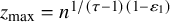 $z_{\max }=n^{1/(\tau -1)(1-\varepsilon _1)}$
this is
$z_{\max }=n^{1/(\tau -1)(1-\varepsilon _1)}$
this is
 $n n^{-(\tau -1-\delta )/(\tau -1)(1-\varepsilon _1)}$
, which has a positive exponent whenever
$n n^{-(\tau -1-\delta )/(\tau -1)(1-\varepsilon _1)}$
, which has a positive exponent whenever
 $\delta>\varepsilon _1(\tau -1)$
. Since
$\delta>\varepsilon _1(\tau -1)$
. Since
 $\varepsilon _1$
was arbitrarily small,
$\varepsilon _1$
was arbitrarily small,
 $\delta $
is thus also arbitrarily small. This, together with a union bound with (A.1) finishes the proof of (15):
$\delta $
is thus also arbitrarily small. This, together with a union bound with (A.1) finishes the proof of (15):
 $$\begin{align*}\begin{aligned} 1-\mathbb{P}(\forall z\ge 1: \nu_n(z) \le z^{-\tau(1-1/\tau+\delta)})&= \mathbb{P}(\exists i\le n: D_i> z_{\max}(\varepsilon_1)) \\ &\qquad+ \mathbb{P}\big(\exists z \le z_{\max}(\varepsilon_1): \nu_n(z) \le z^{-\tau(1-1/\tau+\delta)}\big) \\ &\le n^{1-(1-\varepsilon')/(1- \varepsilon_1)}+n^{1/(\tau-1)(1-\varepsilon_1))} \exp(- n^{\delta}) \to 0. \end{aligned} \end{align*}$$
If one considers truncated power-law distributions with maximal degree
 $z_{\max ,\mathrm {tr}}=o(n^{1/\tau })$
, then
$z_{\max ,\mathrm {tr}}=o(n^{1/\tau })$
, then
 $n z_{\max , \mathrm {tr}}^{-\tau (1-\varepsilon )}\to \infty $
for all possible values z, hence the proof above works with
$n z_{\max , \mathrm {tr}}^{-\tau (1-\varepsilon )}\to \infty $
for all possible values z, hence the proof above works with
 $\varepsilon>0$
arbitrary.
$\varepsilon>0$
arbitrary.
A.2 Proof of long survival on stars
Proof of Claim 6.6.
Denote the neighbors of v by
 $w_1,\ldots ,w_K$
. Define
$w_1,\ldots ,w_K$
. Define
 $$ \begin{align*} \mathcal{A}_1&=\{\xi^v_t(v)=1\text{ for all }t\in[0,1]\},\\ \mathcal{A}_2&=\left\{\left|\left\{i:\xi^v_1(w_i)=1\right\}\right|\ge\lambda K^{1-\mu}/(4e)\right\}. \end{align*} $$
Since v recovers at rate
 $1$
,
$1$
,
 $\mathbb {P}(\mathcal {A}_1\mid \xi _0(v)=1)=1/e$
. Conditioning on
$\mathbb {P}(\mathcal {A}_1\mid \xi _0(v)=1)=1/e$
. Conditioning on
 $\mathcal {A}_1$
, v infects each of
$\mathcal {A}_1$
, v infects each of
 $w_i$
during
$w_i$
during
 $[0,1]$
with rate
$[0,1]$
with rate
 $\lambda K^{-\mu }$
, independently of each other. Hence, for
$\lambda K^{-\mu }$
, independently of each other. Hence, for
 $i=1,\ldots ,K$
,
$i=1,\ldots ,K$
,
 $$ \begin{align*} \mathbb{P}(v\text{ infects } w_i \text{ at some }t\in[0,1])=1-e^{-\lambda K^{-\mu}}\ge\lambda K^{-\mu}/2, \end{align*} $$
using that
 $\lambda K^{-\mu }<1$
. Each
$\lambda K^{-\mu }<1$
. Each
 $u_i$
that becomes infected during
$u_i$
that becomes infected during
 $[0,1]$
is still infected at time
$[0,1]$
is still infected at time
 $1$
with conditional probability at least
$1$
with conditional probability at least
 $1/e$
. Hence,
$1/e$
. Hence,
 $$ \begin{align*} \left|\left\{i:\xi^v_1(w_i)=1\right\}\right| \mid \mathcal{A}_1 \succcurlyeq X\sim \mathrm{Bin}\left(K, \lambda K^{-\mu}/(2e)\right), \end{align*} $$
where
 $\succcurlyeq $
stands for stochastic domination. By a standard Chernoff bound, this yields
$\succcurlyeq $
stands for stochastic domination. By a standard Chernoff bound, this yields
 $$ \begin{align} \mathbb{P}(\mathcal{A}_2\mid \mathcal{A}_1)&\ge\mathbb{P}\left(X\ge \lambda K^{1-\mu}/(4e)\right)\ge 1-e^{-\lambda K^{1-\mu}/(16e)}. \end{align} $$
Therefore,
 $$ \begin{align*} \mathbb{P}(\mathcal{A}_2)\ge \mathbb{P}(\mathcal{A}_1)\cdot\mathbb{P}(\mathcal{A}_2\mid \mathcal{A}_1)\ge \left(1- e^{-\lambda K^{1-\mu}/(16e)}\right)/e, \end{align*} $$
finishing the proof of (117) in Claim 6.6.
We now turn to proving (118) and (119). Starting from time 0, we declare each unit time-interval
 $[s,s+1]$
for
$[s,s+1]$
for
 $s\in {\mathbb {N}}$
successful if the following events jointly occur:
$s\in {\mathbb {N}}$
successful if the following events jointly occur:
 $$ \begin{align} \begin{aligned} \mathcal{B}^1_s&=\left\{\left|\left\{i:\xi_s(w_i)=1\right\}\right|\ge\lambda K^{1-\mu}/(8e)\right\},\\ \mathcal{B}^2_s&=\left\{\left|\left\{i:\xi_t(w_i)=1\text{ for all }t\in[s,s+1]\right\}\right|\ge \lambda K^{1-\mu}/(16e^2)\right\},\\ \mathcal{B}^3_s&=\left\{\int_s^{s+1}\xi_t(v)\,\mathrm{d}t\ge 0.55 \right\},\\ \mathcal{B}^4_s&=\left\{\left|\left\{i:\xi_{s+1}(w_i)=1\right\}\right|\ge \lambda K^{1-\mu}/(8e)\right\}. \end{aligned} \end{align} $$
Here
 $\mathcal {B}^1_s$
is the event that a large enough number of leaves of the star are infected at the beginning of the time interval
$\mathcal {B}^1_s$
is the event that a large enough number of leaves of the star are infected at the beginning of the time interval
 $[s,s+1]$
, which will be enough to sustain the infestation during the whole period, while
$[s,s+1]$
, which will be enough to sustain the infestation during the whole period, while
 $\mathcal {B}^4_s$
is the corresponding event for the end of the time interval.
$\mathcal {B}^4_s$
is the corresponding event for the end of the time interval.
 $\mathcal {B}^2_s$
is the event that the star is infested during
$\mathcal {B}^2_s$
is the event that the star is infested during
 $[s,s+1]$
, while
$[s,s+1]$
, while
 $\mathcal {B}^3_s$
is the event that the center is infected a bit more than half the time during the time interval
$\mathcal {B}^3_s$
is the event that the center is infected a bit more than half the time during the time interval
 $[s,s+1]$
. Note that
$[s,s+1]$
. Note that
 $\mathcal {B}^4_{s}=\mathcal {B}^1_{s+1}$
for all s and that
$\mathcal {B}^4_{s}=\mathcal {B}^1_{s+1}$
for all s and that
 $\mathcal {B}_0^1$
holds by the condition of the Lemma.
$\mathcal {B}_0^1$
holds by the condition of the Lemma.
One can see that if
 $\mathcal {B}_s^1\cap \mathcal {B}_s^2\cap \mathcal {B}_s^3\cap \mathcal {B}_s^4$
holds for all
$\mathcal {B}_s^1\cap \mathcal {B}_s^2\cap \mathcal {B}_s^3\cap \mathcal {B}_s^4$
holds for all
 $s\in \{0,1,\dots , \lfloor T_K\rfloor \}$
, given that
$s\in \{0,1,\dots , \lfloor T_K\rfloor \}$
, given that
 $|\xi _0|\ge \lambda K^{1-\mu }/8\mathrm {e}$
, then the event on the left-hand side of (119) holds (we demand in
$|\xi _0|\ge \lambda K^{1-\mu }/8\mathrm {e}$
, then the event on the left-hand side of (119) holds (we demand in
 $\mathcal {B}_s^3$
a little bit more than
$\mathcal {B}_s^3$
a little bit more than
 $1/2$
of the time being infected, so that even if v is healthy during
$1/2$
of the time being infected, so that even if v is healthy during
 $[\lfloor T_K\rfloor , T_K$
, this does not cause a problem on the total infected time being above
$[\lfloor T_K\rfloor , T_K$
, this does not cause a problem on the total infected time being above
 $T_K/2$
. Further, (118) is a direct consequence of (119), so it is enough to bound the probability of the intersection of these events.
$T_K/2$
. Further, (118) is a direct consequence of (119), so it is enough to bound the probability of the intersection of these events.
We now fix some
 $s\in {\mathbb {N}}$
and bound the conditional probabilities of each of these events given the previous ones. First, any leaf of the star that is infected at time s will stay infected during the whole interval
$s\in {\mathbb {N}}$
and bound the conditional probabilities of each of these events given the previous ones. First, any leaf of the star that is infected at time s will stay infected during the whole interval
 $[s,s+1]$
with conditional probability at least
$[s,s+1]$
with conditional probability at least
 $1/e$
, conditioned on any trajectory of the process on the other vertices. Formally, for any
$1/e$
, conditioned on any trajectory of the process on the other vertices. Formally, for any
 $i=1,\ldots ,K$
,
$i=1,\ldots ,K$
,
 $$ \begin{align*} \inf_{\eta}\mathbb{P}\left(\begin{array}{l}\xi_{t}(w_i)=1\text{ for all }t\in[s,s+1] \mid \xi_s(w_i)=1,\\ \xi\equiv\eta \text{ on } [s,s+1] \text{ on all vertices apart from } u_i\end{array}\right)\ge 1/e. \end{align*} $$
Hence, by a Chernoff bound similar to (A.5),
 $$ \begin{align} \mathbb{P}(\mathcal{B}^2_s \mid \mathcal{B}^1_s)\ge 1-e^{-\lambda K^{1-\mu}/(64e^2)}. \end{align} $$
We will now give a bound on
 $\mathbb {P}(\mathcal {B}_s^3\mid \mathcal {B}_s^1\cap \mathcal {B}_s^2)$
, using that an infested star has enough leaves infected at every time to send back the infection to the center frequently enough to keep it infected for at least half of the time. Formally, given
$\mathbb {P}(\mathcal {B}_s^3\mid \mathcal {B}_s^1\cap \mathcal {B}_s^2)$
, using that an infested star has enough leaves infected at every time to send back the infection to the center frequently enough to keep it infected for at least half of the time. Formally, given
 $\mathcal {B}^1_s\cap \mathcal {B}^2_s$
,
$\mathcal {B}^1_s\cap \mathcal {B}^2_s$
,
 $(\xi _t(v))_{t\in [s,s+1]}$
is a Markov process on the state space
$(\xi _t(v))_{t\in [s,s+1]}$
is a Markov process on the state space
 $\{0,1\}$
with transition rates
$\{0,1\}$
with transition rates
 $$\begin{align*}Q_{01}\ge\lambda K^{1-\mu}\cdot\lambda K^{-\mu}/(16e^2)=\lambda^2 K^{1-2\mu}/(16e^2),\quad\quad Q_{10}=1,\end{align*}$$
and some starting state
 $\xi _s(v)$
. Let us introduce auxiliary Markov processes
$\xi _s(v)$
. Let us introduce auxiliary Markov processes
 $(Y_t)_{t\ge 0}$
,
$(Y_t)_{t\ge 0}$
,
 $(Y^{\prime }_t)_{t\ge 0}$
and
$(Y^{\prime }_t)_{t\ge 0}$
and
 $(Y^{\prime \prime }_t)_{t\ge 0}$
on
$(Y^{\prime \prime }_t)_{t\ge 0}$
on
 $\{0,1\}$
, all starting from the same initial state
$\{0,1\}$
, all starting from the same initial state
 $\xi _s(v)$
, with transition rates
$\xi _s(v)$
, with transition rates
 $$\begin{align*}\begin{array}{lllll} q_{01}&=\lambda^2 K^{1-2\mu}/(16e^2),\quad\quad & q_{10}&=1\quad\quad&\text{of } Y,\\q^{\prime}_{01}&=1,\quad\quad& q^{\prime}_{10}&=16e^2/(\lambda^2 K^{1-2\mu})\quad\quad&\text{of } Y',\\q^{\prime\prime}_{01}&=1,\quad\quad& q^{\prime\prime}_{10}&=1/2\quad\quad&\text{of } Y", \end{array} \end{align*}$$
respectively. Note that
 $Y'$
is a time-changed (slowed-down) version of Y, and
$Y'$
is a time-changed (slowed-down) version of Y, and
 $Y"$
is stochastically dominated by
$Y"$
is stochastically dominated by
 $Y'$
when
$Y'$
when
 $(16e^2)/(\lambda ^2 K^{1-2\mu })<1/2$
. Then, recalling (A.6), we have
$(16e^2)/(\lambda ^2 K^{1-2\mu })<1/2$
. Then, recalling (A.6), we have
 $$ \begin{align}\nonumber \mathbb{P}(\mathcal{B}_s^3\mid \mathcal{B}_s^1\cap\mathcal{B}_s^2)&\ge\mathbb{P}\left(\int_0^1 Y_t\,\mathrm{d}t\ge0.55\right)=\mathbb{P}\left(\frac{16e^2}{\lambda^2 K^{1-2\mu}}\int_0^{\frac{\lambda^2 K^{1-2\mu}}{16e^2}}Y^{\prime}_t\,\mathrm{d}t\ge0.55\right)\\ &\ge\mathbb{P}\left(\frac{16e^2}{\lambda^2 K^{1-2\mu}}\int_0^{\frac{\lambda^2 K^{1-2\mu}}{16e^2}}Y^{\prime\prime}_t\,\mathrm{d}t\ge0.55\right). \end{align} $$
Note that the stationary distribution of
 $Y"$
is
$Y"$
is
 $(\pi _0,\pi _1)=(1/3,2/3)$
. The large deviation principle for Markov chains (see for example [Reference Dembo and Zeitouni22]) yields that the time average of
$(\pi _0,\pi _1)=(1/3,2/3)$
. The large deviation principle for Markov chains (see for example [Reference Dembo and Zeitouni22]) yields that the time average of
 $Y^{\prime \prime }_t$
on the right-hand side of (A.8) is close to
$Y^{\prime \prime }_t$
on the right-hand side of (A.8) is close to
 $\pi _1$
with large probability, as
$\pi _1$
with large probability, as
 $K\to \infty $
:
$K\to \infty $
:
 $$ \begin{align} \mathbb{P}\left(\frac{16e^2}{\lambda^2 K^{1-2\mu}}\int_0^{\frac{\lambda^2 K^{1-2\mu}}{16e^2}}Y^{\prime\prime}_t\,\mathrm{d}t\ge0.55\right)\ge 1-\exp\{-c\lambda^2 K^{1-2\mu}\}. \end{align} $$
Combining (A.8) and (A.9) gives
 $$ \begin{align} \mathbb{P}(\mathcal{B}^3_s \mid \mathcal{B}^1_s\cap \mathcal{B}^2_s)\ge 1-\exp\{-c\lambda^2 K^{1-2\mu}\} \end{align} $$
for some
 $c>0$
.
$c>0$
.
Given
 $\mathcal {B}^3_s$
, during
$\mathcal {B}^3_s$
, during
 $[s,s+1]$
, v spends at least
$[s,s+1]$
, v spends at least
 $1/2$
time in total in state
$1/2$
time in total in state
 $1$
, during which it infects all the leaves with rate
$1$
, during which it infects all the leaves with rate
 $\lambda K^{1-\mu }$
. Each leaf infected this way is still infected at
$\lambda K^{1-\mu }$
. Each leaf infected this way is still infected at
 $s+1$
with conditional probability at least
$s+1$
with conditional probability at least
 $1/e$
. Hence, for
$1/e$
. Hence, for
 $\mathcal {B}_s^4$
given by (A.6), another Chernoff bound, similar to (A.5), yields
$\mathcal {B}_s^4$
given by (A.6), another Chernoff bound, similar to (A.5), yields
 $$ \begin{align} \mathbb{P}(\mathcal{B}^4_s \mid \mathcal{B}^1_s\cap \mathcal{B}^2_s\cap \mathcal{B}^3_s)\ge 1-e^{-\lambda K^{1-\mu}/(32e)}. \end{align} $$
Combining (A.7), (A.10) and (A.11) yields
 $$ \begin{align} \mathbb{P}(\mathcal{B}^1_s\cap \mathcal{B}^2_s\cap \mathcal{B}^3_s\cap \mathcal{B}^4_s \mid \mathcal{B}^1_s)\ge 1-\exp\{-c'\lambda^2K^{1-2\mu}\} \end{align} $$
for some
 $c'>0$
. In words, (A.12) states the following: given that a large enough number of leaves (at least
$c'>0$
. In words, (A.12) states the following: given that a large enough number of leaves (at least
 $\lambda K^{1-\mu }/(8e)$
) are infected at time s, the conditional probability that the time-interval
$\lambda K^{1-\mu }/(8e)$
) are infected at time s, the conditional probability that the time-interval
 $[s,s+1]$
will be successful (in the sense discussed around (A.6)) is at least
$[s,s+1]$
will be successful (in the sense discussed around (A.6)) is at least
 $1-\exp \{-c'\lambda ^2K^{1-2\mu }\}$
. The fact that the time-interval
$1-\exp \{-c'\lambda ^2K^{1-2\mu }\}$
. The fact that the time-interval
 $[s,s+1]$
is successful includes the event
$[s,s+1]$
is successful includes the event
 $\mathcal {B}^4_s=\mathcal {B}^1_{s+1}$
, that is, that a large enough number of leaves are infected at time
$\mathcal {B}^4_s=\mathcal {B}^1_{s+1}$
, that is, that a large enough number of leaves are infected at time
 $s+1$
as well. Hence, using (A.12) iteratively (for
$s+1$
as well. Hence, using (A.12) iteratively (for
 $s=0, 1, \ldots $
) shows that, given
$s=0, 1, \ldots $
) shows that, given
 $\mathcal {B}^1_0=\{|{\underline {\xi }}_0|\ge \lambda K^{1-\mu }/(8e)\}$
, the number of consecutive successful time-intervals
$\mathcal {B}^1_0=\{|{\underline {\xi }}_0|\ge \lambda K^{1-\mu }/(8e)\}$
, the number of consecutive successful time-intervals
 $[0,1], [1,2], \ldots $
stochastically dominates a Geometric random variable with parameter
$[0,1], [1,2], \ldots $
stochastically dominates a Geometric random variable with parameter
 $\exp \{-c'\lambda ^2 K^{1-2\mu }\}$
. Consequently (using a union bound with (A.12)), there exists a constant
$\exp \{-c'\lambda ^2 K^{1-2\mu }\}$
. Consequently (using a union bound with (A.12)), there exists a constant
 $c_1>0$
such that, with
$c_1>0$
such that, with
 $T_K:=\exp (c_1\lambda ^2 K^{1-2\mu })$
,
$T_K:=\exp (c_1\lambda ^2 K^{1-2\mu })$
,
 $$ \begin{align}\nonumber \mathbb{P}\Bigg([0,1],& [1,2], \ldots, [\lfloor T_K\rfloor, \lceil T_K \rceil]\text{ are all successful time-intervals}\ \Big|\ |{\underline{\xi}}_0|\ge \lambda K^{1-\mu}/(8e)\Bigg)\\ &\ge 1-\exp(-c_1\lambda^2 K^{1-2\mu}). \end{align} $$
Recalling how successful time intervals are defined in terms of the events in (A.6), (A.13) implies both (118) and (119) in the claim.
A.3 Proofs about the degrees in the configuration model
Proof of Lemma 7.5.
We will consider ![]() which gives the number of vertices with degree i in
which gives the number of vertices with degree i in
 $G_n[\mathcal {V}_{\le M}]$
. Then the (random) empirical mass function of
$G_n[\mathcal {V}_{\le M}]$
. Then the (random) empirical mass function of
 $\widetilde F_{n,M}$
can be written as
$\widetilde F_{n,M}$
can be written as
 $$ \begin{align} X_{n,M}(i)=\mathbb{P}(\widetilde D_{n,M}=i\mid G_n[\mathcal{V}_{\le M}]) = \frac{\widetilde n_i}{V_{\le M}} = \Big(\frac{V_{\le M}}{n}\Big)^{-1} \cdot \frac{\widetilde n_i}{n}. \end{align} $$
We can now analyze both factors on the rhs separately. The first factor is already given by (141), and can be exactly described using
 $D_n$
with cdf in (8)
$D_n$
with cdf in (8)
 $$ \begin{align} \frac{V_{\le M}}{n} = \frac{n F_n(M)}{n}=F_n(M)=\mathbb{P}(D_n\le M). \end{align} $$
By the definition of
 $\delta _n$
in (147), this falls in the range
$\delta _n$
in (147), this falls in the range
 $\mathbb {P}(D\le M)\pm M\delta _n$
. Turning to the second factor
$\mathbb {P}(D\le M)\pm M\delta _n$
. Turning to the second factor
 $\widetilde n_i/n$
in (A.14), we introduce
$\widetilde n_i/n$
in (A.14), we introduce ![]() the number of degree-
the number of degree-
 $\ell $
vertices in the original graph. Then we can carry out a first and second moment method, that is, we take expectation over the realization of the matching and hence the graph
$\ell $
vertices in the original graph. Then we can carry out a first and second moment method, that is, we take expectation over the realization of the matching and hence the graph
 $G_n[\mathcal {V}_{\le M}]$
. We start with the first moment:
$G_n[\mathcal {V}_{\le M}]$
. We start with the first moment:

To analyze
 $\mathbb {P}(\widetilde d_v=i \mid d_v=\ell )$
, we first deal with self-loops at
$\mathbb {P}(\widetilde d_v=i \mid d_v=\ell )$
, we first deal with self-loops at
 $v\in \mathcal {V}_{\ell }$
. Labeling the half-edges of v as
$v\in \mathcal {V}_{\ell }$
. Labeling the half-edges of v as
 $h_1, h_2, \dots , h_\ell $
, the number of self-loops at v is
$h_1, h_2, \dots , h_\ell $
, the number of self-loops at v is ![]() , with
, with
 $\leftrightarrow $
standing for the event that the two half-edges are matched to each other. We denote the total number of half-edges in the graph by
$\leftrightarrow $
standing for the event that the two half-edges are matched to each other. We denote the total number of half-edges in the graph by
 $H_n=\mathbb {E}[D_n]n$
, and then a first moment method yields, as
$H_n=\mathbb {E}[D_n]n$
, and then a first moment method yields, as
 $\ell \le M$
,
$\ell \le M$
,
 $$ \begin{align} \mathbb{P}( S_v\ge 1 ) \le \mathbb{E}[S_v] = \binom{\ell}{2} \frac{1}{H_n-1}\le \frac{M^2}{\mathbb{E}[D_n] n}. \end{align} $$
Recall from (141) in Definition 7.2 that we denote by
 $H_{\le M}$
and
$H_{\le M}$
and
 $H_{>M}$
the number of half-edges attached to vertices of degree at most M and larger than M, respectively. Partition now the
$H_{>M}$
the number of half-edges attached to vertices of degree at most M and larger than M, respectively. Partition now the
 $\ell $
half-edges of v into (arbitrary) two groups of size i and
$\ell $
half-edges of v into (arbitrary) two groups of size i and
 $\ell -i$
, respectively:
$\ell -i$
, respectively:
 $h_{s_1}, \dots , h_{s_i}$
and
$h_{s_1}, \dots , h_{s_i}$
and
 $h_{s_{i+1}}, \dots , h_{s_\ell }$
, and let us write informally
$h_{s_{i+1}}, \dots , h_{s_\ell }$
, and let us write informally
 $$ \begin{align*} \mathcal{A}_{\{s_1, \dots, s_i\}}:=\Big\{ \{h_{s_1}, \dots, h_{s_i}\} \leftrightarrow \mathcal{V}_{\le M}, \{h_{s_{i+1}}, \dots, h_{s_\ell}\}\leftrightarrow \mathcal{V}_{>M}, S_v=0 \Big\} \end{align*} $$
for the event that the half-edges
 $h_{s_1}, \dots , h_{s_i}$
are all matched to half-edges belonging to vertices in
$h_{s_1}, \dots , h_{s_i}$
are all matched to half-edges belonging to vertices in
 $\mathcal {V}_{\le M}$
, the half-edges
$\mathcal {V}_{\le M}$
, the half-edges
 $h_{s_{i+1}}, \dots , h_{s_\ell }$
are all matched to half-edges belonging to vertices in
$h_{s_{i+1}}, \dots , h_{s_\ell }$
are all matched to half-edges belonging to vertices in
 $\mathcal {V}_{> M}$
, and there is no self-loop created among
$\mathcal {V}_{> M}$
, and there is no self-loop created among
 $h_{s_1}, \dots , h_{s_i}$
. Then, matching half-edges one by one, we come to
$h_{s_1}, \dots , h_{s_i}$
. Then, matching half-edges one by one, we come to
 $$\begin{align*}\begin{aligned} \mathbb{P}(\mathcal{A}_{\{s_1, \dots, s_i\}}) &=\prod_{a=0}^{i-1} \frac{H_{\le M}-\ell-a}{H_n-2a-1} \cdot \prod_{b=0}^{\ell-i-1} \frac{H_{> M}-b}{H_n-2(i+b)-1}. \end{aligned} \end{align*}$$
Observe that per definition ![]() and
and
 $H_n=n\mathbb {E}[D_n]$
so one can compute, using also that
$H_n=n\mathbb {E}[D_n]$
so one can compute, using also that
 $\ell \le M$
, that each factor in the first product is
$\ell \le M$
, that each factor in the first product is
 $q_{n,M}(1+O(M/n))$
and each factor in the second product is
$q_{n,M}(1+O(M/n))$
and each factor in the second product is
 $(1-q_{n,M})(1+O(M/n))$
. Considering all the possible partitions of the half-edges into two groups of i and
$(1-q_{n,M})(1+O(M/n))$
. Considering all the possible partitions of the half-edges into two groups of i and
 $\ell -i$
half-edges, and using that there are
$\ell -i$
half-edges, and using that there are
 $\ell \le M$
factors in the two products together, we arrive at
$\ell \le M$
factors in the two products together, we arrive at
 $$ \begin{align} \begin{aligned} \mathbb{P}(\widetilde d_v=i\mid d_v=\ell) &\ge \sum_{\{s_1, \dots, s_i\}\subset [\ell] } \mathbb{P}\big(\mathcal{A}_{\{s_1, \dots, s_i\}}\big)\\ &= \binom{\ell}{i} q_{n,M}^i (1-q_{n,M})^{\ell-i} \big(1+O\big(\tfrac{M^2}{n}\big)\big). \end{aligned} \end{align} $$
A similar upper bound holds: we account for the error caused by the event that there might be self-loops at v in (A.17),
 $$ \begin{align} \begin{aligned} \mathbb{P}(\widetilde d_v=i\mid d_v=\ell) & \le \mathbb{P}(S_v\ge 1) + \!\!\!\!\!\sum_{\{s_1, \dots, s_i\}\subset [\ell] } \mathbb{P}\big(\mathcal{A}_{\{s_1, \dots, s_i\}}\big)\\ &= O\big(\tfrac{M^2}{n}\big) + \binom{\ell}{i} q_{n,M}^i (1-q_{n,M})^{\ell-i} \big(1+O\big(\tfrac{M^2}{n}\big)\big). \end{aligned} \end{align} $$
Using these bounds in (A.16), and that
 $|\mathcal {V}_\ell |/n=\mathbb {P}(D_n=\ell )$
, we arrive at
$|\mathcal {V}_\ell |/n=\mathbb {P}(D_n=\ell )$
, we arrive at
 $$ \begin{align*} \begin{aligned} \frac{1}{n}\mathbb{E}[\widetilde n_i]&= \sum_{\ell=i}^M\mathbb{P}(D_n=\ell)\bigg(O\big(\tfrac{M^2}{n}\big) + \binom{\ell}{i} q_{n,M}^i (1-q_{n,M})^{\ell-i} \big(1+O\big(\tfrac{M^2}{n}\big)\big)\bigg)\\ &=O\big(\tfrac{M^2}{n}\big) \mathbb{P}(D_n\le M)+ \big(1+O\big(\tfrac{M^2}{n}\big)\big) \sum_{\ell=i}^M\mathbb{P}(D_n=\ell) \binom{\ell}{i} q_{n,M}^i (1-q_{n,M})^{\ell-i}. \end{aligned} \end{align*} $$
Combining this with (A.14) and (A.15), (recalling also that given
 $(d_1, \dots d_n)$
,
$(d_1, \dots d_n)$
,
 $V_{<M}$
is deterministic), we obtain that
$V_{<M}$
is deterministic), we obtain that
 $$ \begin{align} \begin{aligned} \mathbb{E}[X_{n,M}(i)]&=\frac{1}{V_{\le M}}\mathbb{E}[\widetilde n_i]\\ &=O\big(\tfrac{M^2}{n}\big) + \big(1+O\big(\tfrac{M^2}{n}\big)\big) \sum_{\ell=i}^M\frac{\mathbb{P}(D_n=\ell)}{\mathbb{P}(D_n\le M)} \binom{\ell}{i} q_{n,M}^i (1-q_{n,M})^{\ell-i}. \end{aligned} \end{align} $$
We can here observe that the rhs gives the probability
 $\mathbb {P}(\mathrm {Bin}(D_n, q_{n,M})=i \mid D_n\le M)$
. Since
$\mathbb {P}(\mathrm {Bin}(D_n, q_{n,M})=i \mid D_n\le M)$
. Since
 $\mathbb {P}(D_n\le M)\to \mathbb {P}(D\le M)$
and
$\mathbb {P}(D_n\le M)\to \mathbb {P}(D\le M)$
and
 $q_{n,M}\to q_{M}$
by Assumption 1.10, the rhs of (A.20) tends to
$q_{n,M}\to q_{M}$
by Assumption 1.10, the rhs of (A.20) tends to
 $$ \begin{align} \begin{aligned} \lim_{n\to \infty} \mathbb{E}[X_{n,M}(i)] &=\sum_{\ell=i}^M\frac{\mathbb{P}(D=\ell)}{\mathbb{P}(D\le M)} \binom{\ell}{i} q_{M}^i (1-q_{M})^{\ell-i}\\& = \mathbb{P}(\mathrm{Bin}(D, q_M)=i \mid D\le M)=:\mathbb{P}(\widetilde D_M =i)=:p_M(i), \end{aligned} \end{align} $$
where we recognised that the formula on the right hand-side of the first row equals the second row, which ensures that this is a proper random variable. As
 $p_M(i)$
is
$p_M(i)$
is
 $\lim _{n\to \infty }\mathbb {E}[X_{n,M}(i)]$
, we now set out to prove that the random empirical distribution
$\lim _{n\to \infty }\mathbb {E}[X_{n,M}(i)]$
, we now set out to prove that the random empirical distribution
 $\widetilde F_{n,M}$
– with pointmasses
$\widetilde F_{n,M}$
– with pointmasses
 $X_{n,M}(i)$
at i – converges pointwise for each
$X_{n,M}(i)$
at i – converges pointwise for each
 $i\le M$
to
$i\le M$
to
 $p_M(i)$
, in probability. Then (148) will be the limit random variable in the lemma statement.
$p_M(i)$
, in probability. Then (148) will be the limit random variable in the lemma statement.
To achieve this, first we bound the difference between
 $\mathbb {E}[X_{n,m}(i)]$
and its limit
$\mathbb {E}[X_{n,m}(i)]$
and its limit
 $p_M(i)$
. Recalling the definition of
$p_M(i)$
. Recalling the definition of
 $\delta _n$
from (147) we may write
$\delta _n$
from (147) we may write
 $q_{n,M}=q_M(1\pm \delta _n)$
,
$q_{n,M}=q_M(1\pm \delta _n)$
,
 $1-q_{n,M}=(1-q_M)(1\pm \delta _n)$
and similarly we can use that
$1-q_{n,M}=(1-q_M)(1\pm \delta _n)$
and similarly we can use that
 $\mathbb {P}(D_n=\ell )=\mathbb {P}(D=\ell )(1\pm \delta _n)$
when the limit
$\mathbb {P}(D_n=\ell )=\mathbb {P}(D=\ell )(1\pm \delta _n)$
when the limit
 $\mathbb {P}(D=\ell )$
is nonzero and otherwise
$\mathbb {P}(D=\ell )$
is nonzero and otherwise
 $\mathbb {P}(D_n=\ell )\le \delta _n$
. So, we subtract (A.20) from the right-hand side of the first row in (A.21) to obtain after elementary error-estimates that
$\mathbb {P}(D_n=\ell )\le \delta _n$
. So, we subtract (A.20) from the right-hand side of the first row in (A.21) to obtain after elementary error-estimates that
 $$ \begin{align} \begin{aligned} \big|\mathbb{E}[X_{n,M}(i)] - p_M(i)\big| &\le O\big(\tfrac{M^2}{n}\big) + O\big(\tfrac{M^2}{n}+ M^2 \delta_n\big) \mathbb{P}(\widetilde D_M=i)\\ &=O\big(\tfrac{M^2}{n}+\delta_n M^2\big). \end{aligned} \end{align} $$
This finishes comparing the first moments. We now turn to the variance in (A.14). Clearly
 $$ \begin{align} \mathrm{Var}\Big(X_{n,M}(i)\Big) = \mathrm{Var}\Big(\frac{\widetilde n_i}{V_{\le M}}\Big) = \Big(\frac{V_{\le M}}{n}\Big)^{-2} \cdot \frac{\mathrm{Var}(\widetilde n_i)}{n^2}. \end{align} $$
The first factor on the rhs is
 $\mathbb {P}(D_n\le M)^{-2}$
. Using the indicator representation of
$\mathbb {P}(D_n\le M)^{-2}$
. Using the indicator representation of
 $\widetilde n_i$
, we compute using the covariance formula that
$\widetilde n_i$
, we compute using the covariance formula that
 $$ \begin{align} \begin{aligned} \frac{\mathrm{Var}(\widetilde n_i)}{n^2}=\frac{1}{n^2}\sum_{\ell, \ell'=i}^M \sum_{\substack{v\in \mathcal{V}_{\ell}, \\u\in \mathcal{V}_{\ell'}}}&\Big(\mathbb{P}\big(\widetilde d_v=i, \widetilde d_u=i \mid d_v=\ell, d_u=\ell'\big)\\ &\qquad - \mathbb{P}\big(\widetilde d_v=i, \mid d_v=\ell\big) \mathbb{P}\big(\widetilde d_u=i \mid d_u=\ell'\big)\Big). \end{aligned} \end{align} $$
When
 $u=v$
, the two vertices are the same, the (co)variance is at most
$u=v$
, the two vertices are the same, the (co)variance is at most
 $1$
, and the summation contains only at most n terms, hence the error coming from coinciding
$1$
, and the summation contains only at most n terms, hence the error coming from coinciding
 $u,v$
is
$u,v$
is
 $O(1/n)\mathbb {P}(D_n\le M)$
when summed also over
$O(1/n)\mathbb {P}(D_n\le M)$
when summed also over
 $\ell =\ell '$
. Now we treat the case when
$\ell =\ell '$
. Now we treat the case when
 $u\neq v$
. For
$u\neq v$
. For
 $\mathbb {P}\big (\widetilde d_v=i \mid d_v=\ell \big )$
and
$\mathbb {P}\big (\widetilde d_v=i \mid d_v=\ell \big )$
and
 $\mathbb {P}\big (\widetilde d_u=i \mid d_u=\ell '\big )$
we can use the bounds in (A.18) and (A.19). Similarly to there, we compute the first term
$\mathbb {P}\big (\widetilde d_u=i \mid d_u=\ell '\big )$
we can use the bounds in (A.18) and (A.19). Similarly to there, we compute the first term
 $\mathbb {P}\big (\widetilde d_v=i, \widetilde d_u=i \mid d_v=\ell , d_u=\ell '\big )$
as well. Let
$\mathbb {P}\big (\widetilde d_v=i, \widetilde d_u=i \mid d_v=\ell , d_u=\ell '\big )$
as well. Let
 $S_{u,v}$
denote the number of self-loops at the two vertices
$S_{u,v}$
denote the number of self-loops at the two vertices
 $u, v$
together plus the number of edges between u and v. Then a first moment method yields
$u, v$
together plus the number of edges between u and v. Then a first moment method yields
 $$ \begin{align} \mathbb{P}( S_{u,v}\ge 1 ) \le \mathbb{E}[S_{u,v}] = \frac{1}{H_n-1}\bigg(\binom{\ell}{2} + \binom{\ell'}{2} + \ell \ell'\bigg)\le \frac{2M^2}{\mathbb{E}[D_n] n}. \end{align} $$
Now we label the half-edges
 $h_1^{\scriptscriptstyle {(v)}}, \dots , h_\ell ^{\scriptscriptstyle {(v)}}$
and
$h_1^{\scriptscriptstyle {(v)}}, \dots , h_\ell ^{\scriptscriptstyle {(v)}}$
and
 $h_1^{\scriptscriptstyle {(u)}}, \dots , h_{\ell '}^{\scriptscriptstyle {(u)}}$
of v and u, respectively, and partition them into two subsets each, defined by the index sets
$h_1^{\scriptscriptstyle {(u)}}, \dots , h_{\ell '}^{\scriptscriptstyle {(u)}}$
of v and u, respectively, and partition them into two subsets each, defined by the index sets
 $\{s_1, \dots , s_i\}, \{ s_{i+1}, \dots , s_\ell \}\subset [\ell ]$
and
$\{s_1, \dots , s_i\}, \{ s_{i+1}, \dots , s_\ell \}\subset [\ell ]$
and
 $\{t_1, \dots , t_i\}, \{t_{i+1}, \dots , t_{\ell '}\} \subset [\ell ']$
. We introduce the event
$\{t_1, \dots , t_i\}, \{t_{i+1}, \dots , t_{\ell '}\} \subset [\ell ']$
. We introduce the event
 $$ \begin{align*} \begin{aligned} \mathcal{A}_{\{s_1, \dots, s_i, t_1, \dots, t_i\}}:=\Big\{& \{h^{\scriptscriptstyle{(v)}}_{s_1}, \dots, h_{s_i}^{\scriptscriptstyle{(v)}}, h^{\scriptscriptstyle{(u)}}_{t_1}, \dots, h_{t_i}^{\scriptscriptstyle{(u)}}\} \leftrightarrow \mathcal{V}_{\le M}, \\ &\{h_{s_{i+1}}^{\scriptscriptstyle{(v)}}, \dots, h_{s_\ell}^{\scriptscriptstyle{(v)}}, h_{t_{i+1}}^{\scriptscriptstyle{(u)}}, \dots, h_{t_{\ell'}}^{\scriptscriptstyle{(u)}} \}\leftrightarrow \mathcal{V}_{>M}, S_{u,v}=0 \Big\}, \end{aligned} \end{align*} $$
the event that the half-edges
 $h^{\scriptscriptstyle {(v)}}_{s_1}, \dots , h_{s_i}^{\scriptscriptstyle {(v)}}, h^{\scriptscriptstyle {(u)}}_{t_1}, \dots , h_{t_i}^{\scriptscriptstyle {(u)}}$
are all matched to half-edges belonging to vertices in
$h^{\scriptscriptstyle {(v)}}_{s_1}, \dots , h_{s_i}^{\scriptscriptstyle {(v)}}, h^{\scriptscriptstyle {(u)}}_{t_1}, \dots , h_{t_i}^{\scriptscriptstyle {(u)}}$
are all matched to half-edges belonging to vertices in
 $\mathcal {V}_{\le M}$
, the half-edges
$\mathcal {V}_{\le M}$
, the half-edges
 $h_{s_{i+1}}^{\scriptscriptstyle {(v)}}, \dots , h_{s_\ell }^{\scriptscriptstyle {(v)}}, h_{t_{i+1}}^{\scriptscriptstyle {(u)}}, \dots , h_{t_{\ell '}}^{\scriptscriptstyle {(u)}} $
are all matched to half-edges belonging to vertices in
$h_{s_{i+1}}^{\scriptscriptstyle {(v)}}, \dots , h_{s_\ell }^{\scriptscriptstyle {(v)}}, h_{t_{i+1}}^{\scriptscriptstyle {(u)}}, \dots , h_{t_{\ell '}}^{\scriptscriptstyle {(u)}} $
are all matched to half-edges belonging to vertices in
 $\mathcal {V}_{> M}$
, and there is no self-loop and edge created at and between u and v. Then
$\mathcal {V}_{> M}$
, and there is no self-loop and edge created at and between u and v. Then
 $$ \begin{align*} \begin{aligned} \mathbb{P}(\mathcal{A}_{\{s_1, \dots, s_i, t_1, \dots, t_i\}}) &=\prod_{a=0}^{2i-1} \frac{H_{\le M}-\ell-\ell'-a}{H_n-2a-1} \cdot \prod_{b=0}^{\ell+\ell'-2i-1} \frac{H_{> M}-b}{H_n-2(2i+b)-1}. \end{aligned} \end{align*} $$
Using that
 $\ell , \ell '\le M$
, one can compute that each factor in the first product is
$\ell , \ell '\le M$
, one can compute that each factor in the first product is
 $q_{n,M}(1+O(M/n))$
and each factor in the second product is
$q_{n,M}(1+O(M/n))$
and each factor in the second product is
 $(1-q_{n,M})(1+O(M/n))$
. Hence, similarly to (A.18) and (A.19), summing over all possible partitions, we obtain the lower bound
$(1-q_{n,M})(1+O(M/n))$
. Hence, similarly to (A.18) and (A.19), summing over all possible partitions, we obtain the lower bound
 $$ \begin{align*} \begin{aligned} \mathbb{P}\big(\widetilde d_v=i, &\widetilde d_u=i\mid d_v=\ell, d_u=\ell'\big)\\ &\ge \binom{\ell}{i} q_{n,M}^i (1-q_{n,M})^{\ell-i} \binom{\ell'}{i} q_{n,M}^i (1-q_{n,M})^{\ell'-i}\big(1+O(\tfrac{M^2}{n})\big). \end{aligned} \end{align*} $$
and the upper bound is the same as the rhs with an additive
 $O\big (\tfrac {M^2}{n}\big )$
coming from (A.25). We see that this is the same bound as the one in (A.19), multiplied together for u and v. Hence, returning to (A.24), when we take the difference of the two terms, the summand
$O\big (\tfrac {M^2}{n}\big )$
coming from (A.25). We see that this is the same bound as the one in (A.19), multiplied together for u and v. Hence, returning to (A.24), when we take the difference of the two terms, the summand
 $1$
in the
$1$
in the
 $(1+O\big (\tfrac {M^2}{n}\big ))$
factor cancels, and each summand can be upper bounded as
$(1+O\big (\tfrac {M^2}{n}\big ))$
factor cancels, and each summand can be upper bounded as
 $$ \begin{align*} \begin{aligned} \big|\mathbb{P}\big(\widetilde d_v=i, &\ \widetilde d_u=i\mid d_v=\ell, d_u=\ell'\big) - \mathbb{P}\big(\widetilde d_v=i, \mid d_v=\ell\big)\mathbb{P}\big(\widetilde d_u=i \mid d_u=\ell'\big)\big| \\ &\le O\big(\tfrac{M^2}{n}\big) + O\big(\tfrac{M^2}{n}\big)\binom{\ell}{i} q_{n,M}^i (1-q_{n,M})^{\ell-i} \binom{\ell'}{i} q_{n,M}^i (1-q_{n,M})^{\ell'-i}. \end{aligned} \end{align*} $$
We account for the
 $O(1/n)\mathbb {P}(D_n\le M)$
error coming from
$O(1/n)\mathbb {P}(D_n\le M)$
error coming from
 $u=v$
, and use
$u=v$
, and use
 $|\mathcal {V}_{\ell }|/n=\mathbb {P}(D_n=\ell )$
and
$|\mathcal {V}_{\ell }|/n=\mathbb {P}(D_n=\ell )$
and
 $|\mathcal {V}_{\ell '}|/n=\mathbb {P}(D_n=\ell ')$
, then we obtain in (A.24) that
$|\mathcal {V}_{\ell '}|/n=\mathbb {P}(D_n=\ell ')$
, then we obtain in (A.24) that
 $$ \begin{align*} \begin{aligned} \frac{\mathrm{Var}(\widetilde n_i)}{n^2}&\le O(\tfrac{1}{n})\mathbb{P}(D_n\le M) + O\big(\tfrac{M^2}{n}\big)\sum_{\ell, \ell'=i}^M \mathbb{P}(D_n=\ell)\mathbb{P}(D_n=\ell')\\ &\quad\cdot\left(1+ \binom{\ell}{i} q_{n,M}^i (1-q_{n,M})^{\ell-i} \binom{\ell'}{i} q_{n,M}^i (1-q_{n,M})^{\ell'-i}\right)\\ &\le O(\tfrac{M^2}{n}) \Big( \mathbb{P}(D_n\le M) + 2\mathbb{P}(D_n\le M)^2 \Big), \end{aligned} \end{align*} $$
where the last row is a far-from-sharp upper bound.
Wlog we may assume M is large enough for
 $\mathbb {P}(D_n\le M)\ge 1/2$
to hold. Using the previous inequality in (A.23), and that the first factor there is
$\mathbb {P}(D_n\le M)\ge 1/2$
to hold. Using the previous inequality in (A.23), and that the first factor there is
 $1/\mathbb {P}(D_n\le M)^2$
, we come to
$1/\mathbb {P}(D_n\le M)^2$
, we come to
 $$ \begin{align} \mathrm{Var}\Big(X_{n,M}(i)\Big)\le O(\tfrac{M^2}{n}) \Big( 2+ 1/\mathbb{P}(D_n\le M)\Big) = O(\tfrac{M^2}{n}), \end{align} $$
which is true uniformly in i, that is, the factor
 $O(M^2/n)$
is not depending on i.
$O(M^2/n)$
is not depending on i.
We now are ready to prove the bound in (149) in Lemma 7.5. Recall that
 $X_{n,M}(i):=\widetilde n_i/V_{\le m}=\mathbb {P}(\widetilde D_{n,M}=i\mid G_n[\mathcal {V}_{\le M}])$
. We can replace the supremum on the left-hand side of (149) by a “there exists,” followed by a union bound and a triangle inequality:
$X_{n,M}(i):=\widetilde n_i/V_{\le m}=\mathbb {P}(\widetilde D_{n,M}=i\mid G_n[\mathcal {V}_{\le M}])$
. We can replace the supremum on the left-hand side of (149) by a “there exists,” followed by a union bound and a triangle inequality:
 $$ \begin{align} \begin{aligned} \mathbb{P}&\Big(\sup_{i\le M}\big| X_{n,M}(i)-p_M(i)\big| \ge \varepsilon_n \Big) \le \sum_{i\le M}\mathbb{P}\Big(\big| X_{n,M}(i)-p_{M}(i)\big| \ge \varepsilon_n \Big)\\ &\sum_{i\le M}\bigg(\mathbb{P}\Big(\big| X_{n,M}(i)-\mathbb{E}[X_{n,M}(i)]\big| \ge \varepsilon_n/2 \Big) +\mathbb{P}\Big(\big| \mathbb{E}[X_{n,M}(i)]-p_M(i)\Big| \ge \varepsilon_n/2 \Big)\bigg). \end{aligned} \end{align} $$
The second probability in the second row is either
 $0$
or
$0$
or
 $1$
as it involves only deterministic quantities. Recall that we computed
$1$
as it involves only deterministic quantities. Recall that we computed
 $\mathbb {E}[X_{n,M}(i)]$
in (A.20), and
$\mathbb {E}[X_{n,M}(i)]$
in (A.20), and
 $\lim _{n\to \infty }\mathbb {E}[X_{n,M}(i)]=\mathbb {P}(\widetilde D_M=i):=p_M(i)$
in (A.21) per our definition of
$\lim _{n\to \infty }\mathbb {E}[X_{n,M}(i)]=\mathbb {P}(\widetilde D_M=i):=p_M(i)$
in (A.21) per our definition of
 $p_M(i)$
in (A.21) and (148). By (A.22),
$p_M(i)$
in (A.21) and (148). By (A.22),
 $|\mathbb {E}[X_{n,M}(i)]-p_M(i)|\le O(M^2/n+M^2\delta _n)$
. Thus, whenever
$|\mathbb {E}[X_{n,M}(i)]-p_M(i)|\le O(M^2/n+M^2\delta _n)$
. Thus, whenever
 $\varepsilon _n\gg O(M^2/n+M^2\delta _n)$
(that we assumed in Lemma 7.5), the second probability on the right-hand side is
$\varepsilon _n\gg O(M^2/n+M^2\delta _n)$
(that we assumed in Lemma 7.5), the second probability on the right-hand side is
 $0$
simultaneously for all
$0$
simultaneously for all
 $i\le M$
, for all n is sufficiently large. On each term in the first sum we can apply Chebyshev’s inequality, and use the bound on the variance of
$i\le M$
, for all n is sufficiently large. On each term in the first sum we can apply Chebyshev’s inequality, and use the bound on the variance of
 $X_{n,M}(i)$
in (A.26) as follows:
$X_{n,M}(i)$
in (A.26) as follows:
 $$ \begin{align} \begin{aligned} \mathbb{P}\Big(\sup_{i\le M}\big| X_{n,M}(i)-p_M(i)\big| \ge \varepsilon_n \Big) &\le \sum_{i\le M}\mathbb{P}\Big(\big| X_{n,M}(i)-\mathbb{E}[X_{n,M}(i)]\big| \ge \varepsilon_n/2 \Big) \\ &\le \sum_{i\le M} 4\varepsilon_n^{-2} \mathrm{Var}(X_{n,M}(i)) = O\Big(\tfrac{M^3}{n\varepsilon^{2}_n}\Big), \end{aligned} \end{align} $$
where we summed over
 $i\le M$
to obtain the last bound. The rhs tends to zero as
$i\le M$
to obtain the last bound. The rhs tends to zero as
 $n\to \infty $
by the assumption that
$n\to \infty $
by the assumption that
 $\varepsilon _n \gg 1/\sqrt {n}$
implying
$\varepsilon _n \gg 1/\sqrt {n}$
implying
 $n\varepsilon ^2_n\to \infty $
. This finishes the proof of (149).
$n\varepsilon ^2_n\to \infty $
. This finishes the proof of (149).
Recall that
 $\widetilde D_{n,M}$
denotes a random variable with random mass function
$\widetilde D_{n,M}$
denotes a random variable with random mass function
 $X_{n,M}(i)$
. We compute the limit of the (random) mean of the empirical distribution
$X_{n,M}(i)$
. We compute the limit of the (random) mean of the empirical distribution
 $\widetilde F_{n,M}$
of
$\widetilde F_{n,M}$
of
 $G_{n}[\mathcal {V}_{\le M}]$
using (A.28)
$G_{n}[\mathcal {V}_{\le M}]$
using (A.28)
 $$ \begin{align*} \mathbb{E}\big[ \widetilde D_{n,M} \mid G_{n}[\mathcal{V}_{\le M}]\big] = \sum_{i=1}^M i X_{n,M}(i)\ {\buildrel \mathbb{P} \over \longrightarrow }\ \sum_{i=1}^M ip_M(i) =\mathbb{E}\big[\widetilde D_M\big]. \end{align*} $$
Finally, the fact that
 $G_{n}[\mathcal {V}_{\le M}]$
is a configuration model, conditioned on its vertices and their degrees, follows from the fact that every matching of its half-edges have equal probability under the law of the configuration model
$G_{n}[\mathcal {V}_{\le M}]$
is a configuration model, conditioned on its vertices and their degrees, follows from the fact that every matching of its half-edges have equal probability under the law of the configuration model
 $G_n$
. This finishes the proof of Lemma 7.5.
$G_n$
. This finishes the proof of Lemma 7.5.
Proof of Lemma 7.6.
We analyze now the limiting distribution in (148) under the assumption that the original empirical distribution sequence
 $(F_n)_{n\ge 1}$
satisfies both Assumptions 1.10 and 1.11. In particular, Assumption 1.11 implies that the cdf of the limiting distribution
$(F_n)_{n\ge 1}$
satisfies both Assumptions 1.10 and 1.11. In particular, Assumption 1.11 implies that the cdf of the limiting distribution
 $F_D$
of
$F_D$
of
 $D_n$
satisfies (9) for all
$D_n$
satisfies (9) for all
 $\varepsilon>0$
such that for all
$\varepsilon>0$
such that for all
 $n\ge n_0(\varepsilon )$
, and for all
$n\ge n_0(\varepsilon )$
, and for all
 $z\ge z_0$
that
$z\ge z_0$
that
 $$ \begin{align} \frac{c_\ell}{z^{(\tau-1)(1+\varepsilon)}}\le 1-F_D(z) \le \frac{c_u}{z^{(\tau-1)(1-\varepsilon)}}. \end{align} $$
and
 $\mathbb {E}[D]<\infty $
by assumption. We observe first that
$\mathbb {E}[D]<\infty $
by assumption. We observe first that
 $\widetilde D_M$
in (148) is a binomial thinning of
$\widetilde D_M$
in (148) is a binomial thinning of
 $(D| D\le M)$
, hence
$(D| D\le M)$
, hence
 $\widetilde D_M$
is stochastically dominated from above by
$\widetilde D_M$
is stochastically dominated from above by
 $(D| D\le M)$
. So, by the definition of stochastic domination,
$(D| D\le M)$
. So, by the definition of stochastic domination,
 $$ \begin{align} 1-\widetilde F_{M}(z)=\mathbb{P}(\widetilde D_M>z) \le \mathbb{P}(D > z \mid D\le M) = \frac{(1-F_D(z))-(1-F_D(M))}{F_D(M)}. \end{align} $$
Using now (A.29), estimating the numerator from above and the denominator from below, assuming that M is such that
 $c_uM^{-(\tau -1)/2}\le 1/2$
, for all
$c_uM^{-(\tau -1)/2}\le 1/2$
, for all
 $\varepsilon \in (0, (\tau -1)/2]$
it holds for all
$\varepsilon \in (0, (\tau -1)/2]$
it holds for all
 $z\in [z_0, M]$
that
$z\in [z_0, M]$
that
 $$ \begin{align} 1-\widetilde F_{M}(z)\le \frac{c_u z^{-(\tau-1)(1-\varepsilon)} }{1-c_uM^{-(\tau-1)(1-\varepsilon)}}\le \frac{c_u z^{-(\tau-1)(1-\varepsilon)} }{1-c_uM^{-(\tau-1)/2}}\le 2c_u z^{-(\tau-1)(1-\varepsilon)} \end{align} $$
which finishes the proof of the upper bound in (151) with
 $\widetilde c_u=2c_u$
. For the lower bound in (151) we will also need a lower bound on
$\widetilde c_u=2c_u$
. For the lower bound in (151) we will also need a lower bound on
 $\mathbb {P}(D> z \mid D\le M)$
. Using the rhs of (A.30), estimating the denominator by at most
$\mathbb {P}(D> z \mid D\le M)$
. Using the rhs of (A.30), estimating the denominator by at most
 $1$
, and the numerator using (A.29), we obtain
$1$
, and the numerator using (A.29), we obtain
 $$ \begin{align} \mathbb{P}(D> z \mid D\le M)&\ge c_\ell z^{(\tau-1)(1+\varepsilon)} - c_u M^{-(\tau-1)(1-\varepsilon)} \nonumber\\ &= c_\ell z^{-(\tau-1)(1+\varepsilon)} \big(1- (z^{(\tau-1)(1+\varepsilon)}/M^{(\tau-1)(1-\varepsilon)}) \cdot (c_u/c_\ell)\big). \end{align} $$
Here we require that the second factor is at least, say,
 $1/2$
, which leads to
$1/2$
, which leads to
 $$ \begin{align} \begin{aligned} \mathbb{P}(D> z \mid D\le M)&\ge (c_\ell/2) z^{-(\tau-1)(1+\varepsilon)}\\ \mbox{for all} \quad z &\le (c_\ell/(2c_u))^{\tfrac{1}{(\tau-1)(1+\varepsilon)}} M^{1- \tfrac{2\varepsilon}{1+\varepsilon}}=: \widetilde z^{\prime}_{\max}(M). \end{aligned} \end{align} $$
Observe that even without considering the binomial thinning in (148), one cannot hope to prove a lower bound for z too close to M. Nevertheless,
 $\widetilde z^{\prime }_{\max }(M)$
is growing with M for all
$\widetilde z^{\prime }_{\max }(M)$
is growing with M for all
 $\varepsilon < 1$
, and it gets closer to
$\varepsilon < 1$
, and it gets closer to
 $\Theta (M)$
as
$\Theta (M)$
as
 $\varepsilon $
is smaller, which intuitively means that the sharper bound one has on the tail of D, the sharper bound we can also get on probabilities of D falling in given intervals. Nevertheless, even for
$\varepsilon $
is smaller, which intuitively means that the sharper bound one has on the tail of D, the sharper bound we can also get on probabilities of D falling in given intervals. Nevertheless, even for
 $\varepsilon =0$
, we must require
$\varepsilon =0$
, we must require
 $z\le c_2 M$
for some constant
$z\le c_2 M$
for some constant
 $c_2\le 1$
.
$c_2\le 1$
.
Now we compute the thinning probability in (148):

for some constant
 $c_{u,1}>0$
(that does not depend on M) and a similar lower bound holds
$c_{u,1}>0$
(that does not depend on M) and a similar lower bound holds
 $1-q_M\ge c_{\ell ,1} M^{1-(\tau -1)(1+\varepsilon )}$
. Then, using the Binomial representation in (148), and then stochastic domination of
$1-q_M\ge c_{\ell ,1} M^{1-(\tau -1)(1+\varepsilon )}$
. Then, using the Binomial representation in (148), and then stochastic domination of
 $\mathrm {Bin}(j, q)$
by
$\mathrm {Bin}(j, q)$
by
 $\mathrm {Bin}(j^\star , q)$
when
$\mathrm {Bin}(j^\star , q)$
when
 $j\le j^\star $
, we obtain that for all
$j\le j^\star $
, we obtain that for all
 $j^\star \ge z$
,
$j^\star \ge z$
,
 $$ \begin{align} \begin{aligned} \mathbb{P}(\widetilde D_M\ge z) &=\sum_{j=z}^M \frac{\mathbb{P}(D=j)}{\mathbb{P}(D\le M)} \mathbb{P}\big(\mathrm{Bin}(j,q_M) \ge z\big)\\ &\ge \mathbb{P}\big(\mathrm{Bin}(j^\star, q_M)\ge z \big) \mathbb{P}\big(D\ge j^\star \mid D\le M\big), \end{aligned} \end{align} $$
and we can optimize the value
 $j^\star =j^\star (z)\ge z$
to obtain a sharp enough bound. For the second factor on the rhs we may use (A.33). Moving to the “complement” binomial, we estimate the first factor in (A.35) as
$j^\star =j^\star (z)\ge z$
to obtain a sharp enough bound. For the second factor on the rhs we may use (A.33). Moving to the “complement” binomial, we estimate the first factor in (A.35) as
 $$ \begin{align} \begin{aligned} \mathbb{P}(\mathrm{Bin}(j^\star, q_M)\ge z) &= \mathbb{P}(\mathrm{Bin}(j^\star, 1-q_M) \le j^\star-z) \\ &= 1- \mathbb{P}(\mathrm{Bin}(j^\star, 1-q_M)> j^\star-z). \end{aligned} \end{align} $$
We observe that the thinning probability
 $1-q_M$
in (A.34) tends to zero with M. So, when
$1-q_M$
in (A.34) tends to zero with M. So, when
 $z\le \widetilde z^{\prime }_{\max }/2$
, we may take
$z\le \widetilde z^{\prime }_{\max }/2$
, we may take
 $j^\star (z):=2z$
and use Markov’s inequality on the rhs in (A.36) to obtain
$j^\star (z):=2z$
and use Markov’s inequality on the rhs in (A.36) to obtain
 $$ \begin{align*} 1-\mathbb{P}\big(\mathrm{Bin}(2z, 1-q_M)> z \big) \ge 1-\frac{2z(1-q_M)}{z}=1- 2(1-q_M) \ge 1/2 \end{align*} $$
for all M large enough so that
 $c_{u,1}M^{1-(\tau -1)(1-\varepsilon )}<1/4$
. Using this bound in (A.35), along with (A.33), we obtain for all
$c_{u,1}M^{1-(\tau -1)(1-\varepsilon )}<1/4$
. Using this bound in (A.35), along with (A.33), we obtain for all
 $z<\widetilde z_{\max }/2$
that
$z<\widetilde z_{\max }/2$
that
 $$\begin{align*}\mathbb{P}(\widetilde D_M\ge z)\ge \mathbb{P}\big(D\ge 2z \mid D\le M\big)/2 \ge (c_\ell/4) (2z)^{-(\tau-1)(1+\varepsilon)}, \end{align*}$$
which finishes the proof by choosing
 $$\begin{align*}\widetilde c_\ell:=2^{-(\tau-1)(1+\varepsilon)-2}c_\ell\quad\text{ and }\quad\widetilde z_{\max}(M):=2^{-1}(c_\ell/(2c_u))^{\tfrac{1}{(\tau-1)(1+\varepsilon)}} M^{1- \tfrac{2\varepsilon}{1+\varepsilon}}.\\[-37pt] \end{align*}$$
Competing interests
The authors have no competing interest to declare.
Financial support
ZB was supported by the ERC Consolidator Grant 772466 “NOISE.”
Ethical standards
The research meets all ethical guidelines, including adherence to the legal requirements of the study country.
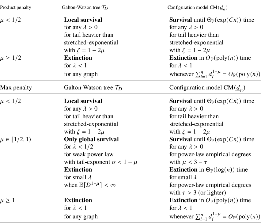


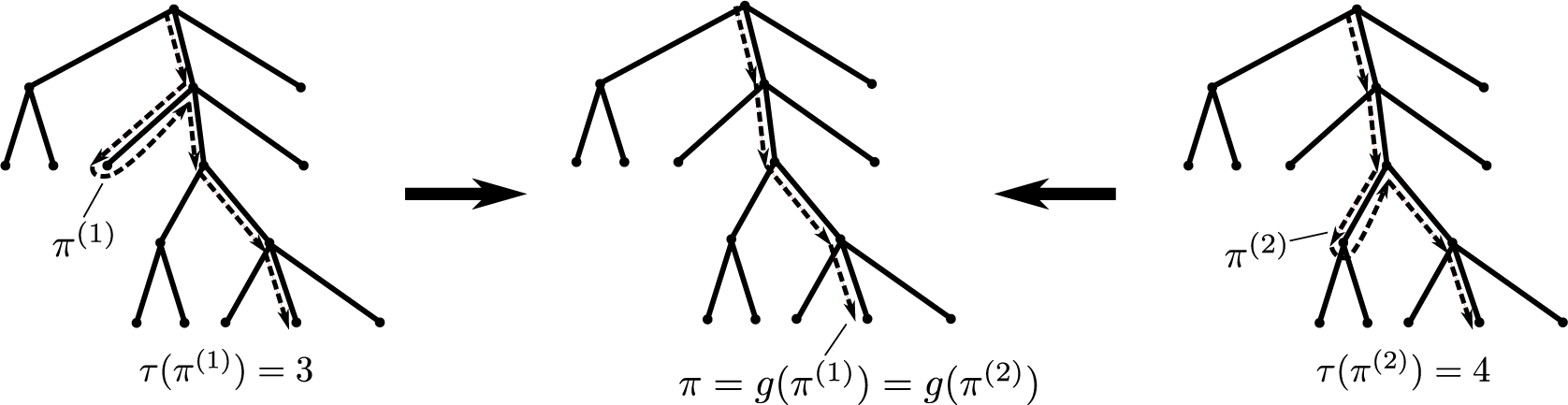


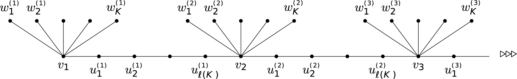

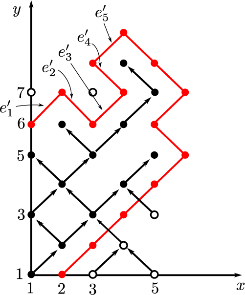


 Open access