


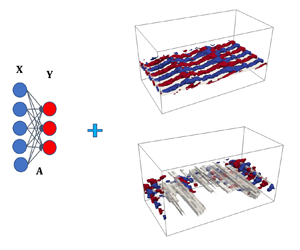



1. Introduction
Modelling turbulent flows and predicting their time evolution, e.g. to assess the performance of different feedback or feedforward control strategies (Noack, Morzynski & Tadmor Reference Noack, Morzynski and Tadmor2011; Brunton & Noack Reference Brunton and Noack2015; Jones et al. Reference Jones, Heins, Kerrigan, Morrison and Sharma2015) is a challenging problem because of the high complexity of the underlying physical problem and the need for large computational resources. The disparate number of spatio-temporal scales involved in the description of turbulent flows calls therefore for a high number of degrees of freedom to define the problem, which soon raises the cost in terms of computational time and memory. During recent years, the community has paid special attention to finding new tools that provide low-rank high-fidelity models describing the main flow dynamics, relate inputs to outputs for flow control (e.g. balanced truncation) and develop models for unexplored physics (Sharma Reference Sharma2011; Lassila et al. Reference Lassila, Manzoni, Quarteroni and Rozza2014; Le Clainche Reference Le Clainche2019; Mendez, Balabane and Buchlin Reference Mendez, Balabane and Buchlin2019).
Data-driven equation-free models are promising tools that can provide accurate descriptions of the flow without a priori knowledge of the underlying equations. Depending on the main objectives, it is possible to identify two types of approaches for data-driven models: (i) models that only focus on data forecasting, using machine learning tools based e.g. on deep neural networks or alternative black-box approaches, and (ii) models that also include some physical insight into the problem to construct a reduced-order model (ROM), e.g. using pattern identification approaches such as proper orthogonal decomposition (Sirovich Reference Sirovich1987) or dynamic mode decomposition (DMD), (Schmid Reference Schmid2010).
Using data-driven ROMs in fluid dynamics provides several advantages compared with purely deep neural networks strategies. These methods extract relevant spatio-temporal information about the physics, which can be used to identify the main instabilities and mechanisms in the flow and/or to create powerful tools for optimization (Park et al. Reference Park, Jun, Baek, Cho, Yee and Lee2013) and control (Gao et al. Reference Gao, Zhang, Kou, Liu and Ye2017). Gaining some additional physical insight into the problem, it is also possible to better predict the system phase state, use more controlled and robust strategies, reduce the computational cost of numerical simulations or limit the information collected in experiments (Le Clainche, Vega & Soria Reference Le Clainche, Vega and Soria2017; Le Clainche & Ferrer Reference Le Clainche and Ferrer2018).
The use of machine learning to reduce the problem dimensionality and to predict state variables is a data-driven strategy rapidly diffusing in the fluid dynamics community, although these tools have already been extensively used for a large number of applications in other fields (Dargan et al. Reference Dargan, Kumar, Ayyagari and Kumar2019). Among these methods, deep learning has recently been introduced as a powerful tool for system identification in fluid dynamics (Brunton, Noack & Koumoutsakos Reference Brunton, Noack and Koumoutsakos2020). Generally, deep-learning algorithms are introduced as a sequence of neural network layers (usually from 9 to 10) trained by optimizing a cost function using gradient descent algorithms (LeCun, Bengio & Hinton Reference LeCun, Bengio and Hinton2015; Lopez-Martin, Carro & Sanchez-Esguevillas Reference Lopez-Martin, Carro and Sanchez-Esguevillas2019). Nevertheless, only simple and general definitions of these algorithms have been used to solve complex fluid dynamics problems. Among the many existing studies, we mention Xiaoxiao, Wei & Iorio (Reference Xiaoxiao, Wei and Iorio2016) who used a convolutional neural network with an encoding/decoding configuration to predict velocity fields for steady flows. Two-dimensional convolutional neural network architectures have also been used by several authors to estimate velocity vectors from a sequence of particle image velocimetry data (Cai et al. Reference Cai, Zhou, Xu and Gao2019, Reference Cai, Liang, Gao, Xu and Wei2020; Lee, Yang & Yin Reference Lee, Yang and Yin2019). Additionally, the use of two-dimensional convolutional neural network methods is also currently being explored by several authors for weather forecasting in combination with dynamical system simulation tools (Scher Reference Scher2018; Agrawal et al. Reference Agrawal, Barrington, Bromberg, Burge, Gazen and Hickey2019; Scher & Messori Reference Scher and Messori2019; Wang, Balaprakash & Kotamarthi Reference Wang, Balaprakash and Kotamarthi2019). For all cases, convolutional neural network approaches show results similar to or better than state of the art models. Wan et al. (Reference Wan, Vlachas, Koumoutsakos and Sapsis2018) used a recurrent neural network to model complex dynamical systems, helping to improve a ROM in regions where the data were known. In the same line of work, Vlachas et al. (Reference Vlachas, Byeon, Wan, Sapsis and Koumoutsakos2019) compared the performance of recurrent neural network and Gaussian processes for forecasting high-dimensional dynamics, the former resulting more accurate. As another alternative to methods based on Gaussian processes, White, Ushizima & Farhat (Reference White, Ushizima and Farhat2019) propose a cluster network to perform simulations in fluid dynamics, although this method requires extensive tuning. Wiewel, Becher & Thuerey (Reference Wiewel, Becher and Thuerey2019), similarly, suggest a model combining convolutional and recurrent layers in an encoder–decoder architecture to predict pressure flow fields. Recently, Lopez-Martin, Le Clainche & Carro (Reference Lopez-Martin, Le Clainche and Carro2020) proposed a new model for predictions in fluid dynamics using three-dimensional convolutional neural networks (with a low-dimensional intermediate latent space) and objectives (k-ahead velocity-field prediction for a synthetic jet), avoiding the use of video sequences. More details about different machine learning techniques and their application to system identification, dimensionality reduction and feature extraction can be found in the review article by Brunton et al. (Reference Brunton, Noack and Koumoutsakos2020).
Currently, different authors are working on the development of new tools combining methods generally used to identify patterns in fluid dynamics and classical deep-learning strategies. For instance, Lusch, Kutz & Brunton (Reference Lusch, Kutz and Brunton2017) combined the Koopman linear embedding representation, which contains information about the physical model, with a modified deep auto-encoder, which is responsible for the high efficiency of a deep neural network; Meena, Nair & Taira (Reference Meena, Nair and Taira2018) proposed a network community-based ROM to predict the lift and drag forces on bodies taking advantage of the vortical interactions. The good performance presented in these previous studies encourages the search for new algorithms that overcome the problems generally found in deep learning, or more specifically, in neural network (NN) architectures applied to fluid dynamic problems. On the one hand, to provide accurate predictions of complex data, NNs are generally composed by several layers and neurons using nonlinear activation functions. On the other hand, the large number of degrees of freedom of fluid dynamic problems requires the generation of large-size databases, leading to highly demanding computational problems (high memory and computational time). Thus, algorithms combining deep learning strategies, such as NNs, with other approaches, for instance based on data dimensionality reduction and containing partial information on the flow physics, appear as a viable alternative.
In the same spirit, the present work takes advantage of the physical insight into the problem studied to construct a ROM. For the first time, to the authors’ knowledge, this article combines the deep learning strategies introduced by Meena et al. (Reference Meena, Nair and Taira2018) with a modal decomposition, specifically DMD modes, representing the main flow instabilities and energy-producing mechanisms modelling the large-scale most-energetic turbulent flow structures. The model proposed is equivalent to a NN architecture formed by a single neuron using a linear activation function. The input data consist of several DMD modes and their multiple nonlinear interactions, which represent the large-scale flow motions. Hence, the DMD modes provide a data dimensionality reduction based on the physics associated with the most energetic flow structures. This new method is applied to approximate the statistics of the wall-shear stress over long time periods in a turbulent channel flow over an anisotropic porous wall. The wall-shear stress has been estimated both in terms of space average and locally over the entire channel wall. Turbulent flows contain chaotic high-frequency information that cannot be predicted by the model proposed, since it uses DMD modes that represent the low-frequency flow motions, i.e. the quasi-coherent flow structures. Nevertheless, the algorithm proposed considers the interaction of the DMD modes, which reproduce the regeneration of new flow structures. In other words, our surrogate model has similar mean, standard deviation and similar frequency spectrum to that of the measured wall-shear stress. In addition, the spectrum contains additional frequencies, induced by the nonlinear interaction of the selected modes, which well match those existing in the flow.
The capability of the methodology used to perform the modal decomposition was already shown in more fundamental turbulent flows by the present authors in Le Clainche et al. (Reference Le Clainche, Izvassarov, Rosti, Brandt and Tammisola2020). In this article, we identified the main spatio-temporal structures in a turbulent channel flow and compared these with the case of elastoviscoplastic fluids. The results presented showed the main flow structures in the three cases identified as spatio-temporal DMD modes. Moreover, these results revealed the role of the near-wall streaks and their breakdown. In this new study, we try to approximate the statistics of the wall-shear stress based on the DMD modes in three cases where turbulence is significantly modified. To keep the paper focused on the new methodology introduced we do not consider classic turbulence on solid walls, see, however, Le Clainche et al. (Reference Le Clainche, Izvassarov, Rosti, Brandt and Tammisola2020) for the analysis of this case. So far, applications of machine learning strategies to turbulent flows have been limited to two-dimensional homogeneous turbulent flow reconstructions (Fukami, Fukagata & Taira Reference Fukami, Fukagata and Taira2020), reducing data dimensions (Omata & Shirayama Reference Omata and Shirayama2019), super-resolution analyses (Fukami, Fukagata & Taira Reference Fukami, Fukagata and Taira2019), predictions of small-scale ocean turbulence (Salehipour & Peltier Reference Salehipour and Peltier2019) or data assimilation (nudging) in three-dimensional homogeneous and isotropic turbulence (Di Leoni, Mazzino & Biferale Reference Di Leoni, Mazzino and Biferale2020). The present article presents a novel algorithm based on modal decompositions and NNs that is able to reconstruct the temporal variations of the wall-shear stress in a complex turbulent flow based on the nonlinear interaction of DMD modes at a reduced computational cost. Namely, once the model is implemented, the computational time to reproduce the statistics of the wall-shear stress for very large periods of time (i.e. 1500 time units) varies from 4 to 20 minutes for the local wall-shear stress all and less than a minute (in some models less than 2 seconds) for the spatially averaged approximations. The simplicity of the model proposed opens the possibility of its extension to any type of flow. The physics encoded in the DMD modes, used as a basis for the reduced model, is explained in detail while comparing the dynamics over an anisotropic porous wall with that over its isotropic counterpart. To accurately approximate the flow evolution, the modal decomposition is connected to a network community, which quantifies the nonlinear interaction of modes in the flow.
The article is organized as follows. Section 2 briefly introduces the numerical simulations of the turbulent channel flow, describing the geometry, the wall porosity and the flow conditions of the data analysed. Section 3 explains the methodology used for the modal decomposition and for identifying the dominant temporal and spatio-temporal DMD modes. The deep-learning model based on modal decomposition is detailed in § 4 and the network community is presented in § 5. Section 6 briefly describes the flow physics related to the DMD modes identified. The performance of the model is introduced in § 7 and the connection of the mode-to-mode interaction with the modularity of the community is presented in § 8. Finally, the main conclusions are presented in § 9.
2. Numerical simulations in a channel with isotropic and anisotropic porous walls
The turbulence modulation over a porous wall has been investigated in the past both numerically and experimentally. Breugem, Boersma & Uittenbogaard (Reference Breugem, Boersma and Uittenbogaard2006) studied the effect of a packed bed of particles on turbulent channel flows and found an increase of turbulent drag associated with a strong reduction of the intensity of the low- and high-speed streaks and of the quasi-streamwise vortices characteristics of wall-bounded flows. These results were later extended by Rosti, Cortelezzi & Quadrio (Reference Rosti, Cortelezzi and Quadrio2015) to porous materials with relatively small permeability, and also verified experimentally by Suga et al. (Reference Suga, Matsumura, Ashitaka, Tominaga and Kaneda2010) and Suga, Nakagawa & Kaneda (Reference Suga, Nakagawa and Kaneda2017). Recently, anisotropic porous walls have received increasing attention, since they may provide an effective means to manipulate turbulence. Gómez-de-Segura, Sharma & García-Mayoral (Reference Gómez-de-Segura, Sharma and García-Mayoral2017), Kuwata & Suga (Reference Kuwata and Suga2017), Rosti, Brandt & Pinelli (Reference Rosti, Brandt and Pinelli2018a) and Kuwata & Suga (Reference Kuwata and Suga2019) assessed the potential of these surfaces; recently, Abderrahaman-Elena & García-Mayoral (Reference Abderrahaman-Elena and García-Mayoral2017) performed an analysis based on the effect of small-scale surface manipulations on near-wall turbulence, predicting a monotonic decrease in skin friction as the streamwise permeability increases. Gómez-de-Segura & García-Mayoral (Reference Gómez-de-Segura and García-Mayoral2019) verified the predictions of Abderrahaman-Elena & García-Mayoral (Reference Abderrahaman-Elena and García-Mayoral2017). Following in the same line, Rosti et al. (Reference Rosti, Izbassarov, Tammisola, Hormozi and Brandt2018b) identified changes in the skin friction when varying the streamwise and spanwise permeabilities.
The database generated and presented in Rosti et al. (Reference Rosti, Izbassarov, Tammisola, Hormozi and Brandt2018b) has been analysed in this article. In this previous work, numerical simulations were carried out to model the main patterns of turbulent channel flows over a porous wall at three different permeability conditions: (i) isotropic wall, (ii) anisotropic wall with higher permeability along the wall-normal direction than along the streamwise and spanwise directions ( $\sigma _y=4$ and $\sigma _{xz}=0.25$ with $\sigma$ being the square root of the permeability divided by the channel half-height i.e. $\sigma =\sqrt {K}/h$), producing a drag increasing (DI) mechanism and (iii) anisotropic wall with lower permeability along the wall-normal direction than along the streamwise and spanwise directions ( $\sigma _y=0.0625$ and $\sigma _{xz}=16$), producing a drag reduction (DR) mechanism. The main set-up of the simulations are presented in Rosti et al. (Reference Rosti, Izbassarov, Tammisola, Hormozi and Brandt2018b), and briefly repeated here for the sake of clarity.
The computational domain consists of a rectangular box with streamwise and spanwise dimensions  $L_x\in [0,4{\rm \pi} ]$ and $L_z\in [0,2{\rm \pi} ]$, respectively, and wall-normal dimension $L_y\in [-0.2,2.2]$, where the thickness of the porous wall is $0.2$, at the top and bottom channel walls, as presented in figure 1, where the coordinate system adopted is also presented and the channel lengths are normalized with $h$ (half the channel height). Periodic boundary conditions are imposed in the streamwise and spanwise directions. The porosity is maintained constant as $\epsilon =0.6$. The bulk Reynolds number is $2800$, defined as $Re=Uh/\nu$, with $U$,
$U$,  $h$ and $\nu$, the bulk streamwise velocity, half the channel height and the kinematic fluid viscosity, respectively, which correspond to a frictional Reynolds, $Re_{\tau }=180$ in the case of rigid walls. Considering the turbulent flow at a constant flow rate, the friction Reynolds number varies depending on the type of porous walls, modifying the length scale of turbulent vortices and complexity of the flow dynamics. The choice was originally made in Rosti et al. (Reference Rosti, Cortelezzi and Quadrio2015, Reference Rosti, Brandt and Pinelli2018a) to ease the comparison of the results of cases with varying permeability with those from an impermeable channel flow case. Here, we use the same dataset and follow the same normalization, the interested reader is referred to these references for more details. The flow within the porous layers is modelled using the volume averaged Navier–Stokes equations (Whitaker Reference Whitaker1969) and the numerical solution based on Fourier discretization in the wall-parallel directions and high-order compact finite differences in the wall-normal one. More details about the numerical code can be found in Rosti et al. (Reference Rosti, Cortelezzi and Quadrio2015). Table 1 summarizes the different cases studied and list the parameters that are physically relevant, see e.g. Rosti et al. (Reference Rosti, Cortelezzi and Quadrio2015).
Computational domain in the channel flow with a porous wall.

Parameters used in the numerical simulations. Value of the resulting friction Reynolds number  $Re_{\tau }=u_\tau h/\nu$ and the two porous Reynolds numbers $Re_{\sigma _{xz}}=\sqrt {K_{xz}} U/\nu$ and $Re_{\sigma _y}=\sqrt {K_{y}} U/\nu$ of the isotropic and anisotropic cases studied for a fixed bulk Reynolds number $Re=2800$, with the corresponding DR.

To provide a first picture of the flows under investigation, we display in figure 2 the streamwise velocity in a wall-parallel plane  $XZ$ near the porous interface for the three different cases. Starting from the isotropic case as reference, one can recognise the near-wall streamwise-correlated structures (streaks). These become more regular and of larger size in the DR case, a feature of many drag-reducing flows where the thickness of the buffer layer increases (Ceccio Reference Ceccio2010) and the flow complexity decreases; in the DI case, conversely, the streaks are characterized by a smaller size and are less organized, indicating an increase of the flow complexity. More specifically, in figure 2(c) (DI) it is difficult to identify the characteristic streamwise-correlated streaks, rather the flow is composed of small-size spatial structures, where it is possible to guess some spanwise correlations (more details will be presented below).
Streamwise velocity in an  $XZ$ plane extracted at the porous interface from the simulations with the isotropic porous wall (a), DR (b) and DI (c) cases. The blue and red colours are used to indicate velocity fluctuations equal to $\pm 0.4 \bar {u}(y=0)$. The flow goes from (a) to (c).

3. Methodology to identify the main flow patterns
This article presents a deep-learning model based on a modal expansion, constructed using a group of DMD modes leading the dynamics at large scale. The physics of turbulence production is captured by means of spatio-temporal DMD modes, periodic along the spanwise direction. This section introduces the techniques to extract and identify DMD and spatio-temporal DMD modes and includes a novel application of these methods for the analysis of turbulent flows. It is important to remark that, as discussed in Chen, Tu & Rowley (Reference Chen, Tu and Rowley2012), the DMD modes correspond to Fourier modes for very large datasets. However, the benefit of using the DMD algorithm presented below (higher-order DMD) compared with the spectral analysis lies in the capabilities of this method to provide highly accurate results using a much smaller number of snapshots (see more details in Le Clainche & Vega Reference Le Clainche and Vega2017a, figure 10).
3.1. Higher-order DMD
Higher-order dynamic mode decomposition (HODMD) (Le Clainche & Vega Reference Le Clainche and Vega2017a) is a data-driven method that decomposes a set of data,  $\boldsymbol {v}_{k}(x,y,z,t)$ (snapshot), as an expansion of DMD modes $\boldsymbol {u}_m(x,y,z)$ (of unit norm) in the following way:
 \begin{equation} \boldsymbol{v}(x,y,z,t_k)\simeq \sum_{m=1}^{M} a_{m}\boldsymbol{u}_m(x,y,z) \,{\rm e}^{(\delta_m+{\rm i} \omega_m)t_k},\quad k=1,\ldots,K, \end{equation}
where  $\omega _m$, $\delta _m$ and $a_{m}$ are the mode frequencies, growth rates and amplitudes, respectively. HODMD is an extension of DMD (Schmid Reference Schmid2010), introduced for the analysis of highly noisy configurations (Le Clainche et al. Reference Le Clainche, Vega and Soria2017) and complex or turbulent flows (Le Clainche et al. Reference Le Clainche, Izvassarov, Rosti, Brandt and Tammisola2020).
Organizing the data evolving in time into a matrix of dimension  $J\times K$, conformed by $K$ snapshots, as
 \begin{equation} V_1^{K} =[\boldsymbol{v}_1,\boldsymbol{v}_2,\ldots,\boldsymbol{v}_k,\ldots,\boldsymbol{v}_K], \end{equation}
where  $\boldsymbol {v}_k$ is the velocity vector collected at time instant $t_k$, of dimension $J\times 1$ ( $J=N_x \times N_y \times N_z$, with $N_x$, $N_y$ and $N_z$ the number of grid points along the streamwise, wall-normal and spanwise spatial components), the algorithm can be summarized in two main steps:
• Step 1: Dimension reduction. Singular value decomposition (SVD) is applied to the snapshot matrix (3.2) as,
(3.3)where \begin{equation} V_1^{K}\simeq U\varSigma T^{\top}= U\hat V_1^{K}, \end{equation}$U^{\top } U = T^{\top } T$ is equal to the $K'\times K'$ identity matrix, $\varSigma$ a diagonal matrix whose elements are the retained singular values $\sigma _i$ and $\hat V_1^{K}=\varSigma T^{\top }$ the so-called reduced snapshot matrix; its columns are conformed by the reduced snapshots, defined as $\hat {\boldsymbol {v}}_k$. The $K'$ singular values are selected according to a tuneable tolerance $\varepsilon _1$ as
(3.4)In other words, the singular values retained satisfy the following equation:\begin{equation} \sigma_{K'+1}/\sigma_{1}\leq \varepsilon_1.\end{equation}$\sigma _{i}/\sigma _{1}> \varepsilon _1$, for $i=1,\ldots, K'$. For complex dynamics (i.e. turbulent flows), the data of the snapshot matrix (3.2) are organized in tensor form as $V(x_i, y_l, z_r, t_k)=V_{ilrk}$; for $i=1,I$; $l=1,L$; $r=1,R$; $k=1,K$ with $I$, $L$ and $R$ being the number of grid points in the spatial directions, $x$, $y$, $z$ with $K$ the snapshot number. Instead of a standard SVD, high-order SVD (Tucker Reference Tucker1966) is applied to this tensor, which is similar to applying SVD to the four matrices whose columns are formed by the tensor fibres (representing each one of the $4$ data variables), as
(3.5)where\begin{equation} V_{ilrk}\simeq\sum_{p_1=1}^{P_1}\sum_{p_2=1}^{P_2}\sum_{p_3=1}^{P_3}\sum_{p_4=1}^{P_4} S_{p_1p_2p_3p_4} W^{(x)}_{ip_1} W^{(y)}_{lp_2} W^{(z)}_{rp_3} T_{kp_4}, \end{equation}$S_{p_1p_2p_3p_4}$ is the core tensor (a fourth-order tensor) and the columns of the matrices $W^{(x)}$, $W^{(y)}$, $W^{(z)}$ and $T$ are the modes of the decomposition (three spatial and one temporal mode, respectively). The dimension reduction, as presented in (3.4), is applied to each one of these modes: this enables us to better remove spurious artefacts such as noise, or small-size flow scales of the turbulent flows (treated hence as noise).
\begin{equation} V_1^{K}\simeq U\varSigma T^{\top}= U\hat V_1^{K}, \end{equation}$U^{\top } U = T^{\top } T$ is equal to the $K'\times K'$ identity matrix, $\varSigma$ a diagonal matrix whose elements are the retained singular values $\sigma _i$ and $\hat V_1^{K}=\varSigma T^{\top }$ the so-called reduced snapshot matrix; its columns are conformed by the reduced snapshots, defined as $\hat {\boldsymbol {v}}_k$. The $K'$ singular values are selected according to a tuneable tolerance $\varepsilon _1$ as
(3.4)In other words, the singular values retained satisfy the following equation:\begin{equation} \sigma_{K'+1}/\sigma_{1}\leq \varepsilon_1.\end{equation}$\sigma _{i}/\sigma _{1}> \varepsilon _1$, for $i=1,\ldots, K'$. For complex dynamics (i.e. turbulent flows), the data of the snapshot matrix (3.2) are organized in tensor form as $V(x_i, y_l, z_r, t_k)=V_{ilrk}$; for $i=1,I$; $l=1,L$; $r=1,R$; $k=1,K$ with $I$, $L$ and $R$ being the number of grid points in the spatial directions, $x$, $y$, $z$ with $K$ the snapshot number. Instead of a standard SVD, high-order SVD (Tucker Reference Tucker1966) is applied to this tensor, which is similar to applying SVD to the four matrices whose columns are formed by the tensor fibres (representing each one of the $4$ data variables), as
(3.5)where\begin{equation} V_{ilrk}\simeq\sum_{p_1=1}^{P_1}\sum_{p_2=1}^{P_2}\sum_{p_3=1}^{P_3}\sum_{p_4=1}^{P_4} S_{p_1p_2p_3p_4} W^{(x)}_{ip_1} W^{(y)}_{lp_2} W^{(z)}_{rp_3} T_{kp_4}, \end{equation}$S_{p_1p_2p_3p_4}$ is the core tensor (a fourth-order tensor) and the columns of the matrices $W^{(x)}$, $W^{(y)}$, $W^{(z)}$ and $T$ are the modes of the decomposition (three spatial and one temporal mode, respectively). The dimension reduction, as presented in (3.4), is applied to each one of these modes: this enables us to better remove spurious artefacts such as noise, or small-size flow scales of the turbulent flows (treated hence as noise).• Step 2: DMD-d algorithm. This algorithm linearly relates snapshots at a given time with the sequential
$d$ time-lagged snapshots at earlier times, using the generalized Koopman assumption,
(3.6)After some calculations (see details in Le Clainche et al. Reference Le Clainche, Vega and Soria2017), the DMD expansion (3.1) for the reduced snapshots can be written as\begin{equation} \hat{\boldsymbol{v}}_{k+d} \simeq R_1 \hat{\boldsymbol{v}}_k + R_2 \hat{\boldsymbol{v}}_{k+1} + \ldots + R_d \hat{\boldsymbol{v}}_{k+d-1}, \quad k = 1, 2, \ldots, K-d. \end{equation}(3.7)where\begin{equation} \hat{\boldsymbol{v}}_k \simeq \sum_{m=1}^{M} \hat a_{m}\hat{\boldsymbol{u}}_{m}\,{\rm e}^{(\delta_{m}+{{\rm i}}\omega_{m}) t_k}, \end{equation}$\hat {\boldsymbol {u}}_{m}$ are the reduced modes (normalized) and $\hat {a}_m$ the reduced amplitudes, calculated by least squares fitting of the two sides of (3.7). The $M$ DMD modes in (3.1) are selected by imposing
(3.8)with\begin{equation} \frac{|\hat a_m|}{\max\{|\hat a_m|\}}>\varepsilon_2, \end{equation}$\varepsilon _2$ a tuneable threshold. Premultiplying both sides of (3.7) by the matrix $U$
(3.9a,b)where\begin{equation} a_m=\frac{|\hat a_m| \|U\hat{\boldsymbol{u}}_{m}\|_2}{\sqrt{J}}, \quad \boldsymbol{u}_{m}=\frac{\hat a_m U\hat{\boldsymbol{u}}_{m}}{a_m}, \end{equation}$\|\cdot \|_2$ is the Euclidean norm, and recalling (3.3), leads to the expansion (3.1).


The high complexity of the data analysed (turbulent flows) encourages the need for combining the HODMD algorithm with other strategies to identify correctly the quasi-coherent flow structures. The iterative HODMD algorithm is therefore applied. This consists of applying HODMD iteratively over the data reconstructed using the DMD expansion (3.1) to progressively remove spurious or smaller-scale modes. In other words, in a first stage, HODMD is applied to the snapshot matrix (3.2) obtaining the DMD expansion (3.1), which is assumed as the new snapshot matrix. HODMD is again applied over this new matrix until the number of retained SVD modes,  $P_1$, $P_2$, $P_3$ and $P_4$ in (3.5), do not change between two consecutive iterations.
3.2. Spatio-temporal Koopman decomposition
Spatio-temporal Koopman decomposition (STKD) (Le Clainche & Vega Reference Le Clainche and Vega2018b) is an extension of HODMD that provides general spatio-temporal DMD expansions, namely assuming periodicity in the spanwise direction
 \begin{align} \boldsymbol{v}(x,y,z_r,t_k)&\simeq \sum_{m=1}^{M}\sum_{n=1}^{N} a_{mn}\boldsymbol{u}_{mn}(x,y)\nonumber\\ &\quad \times {\rm e}^{(\delta_m+{\rm i} \omega_m)t_k+(\nu_{mn}+{\rm i}\beta_{mn})z_r},\quad k=1,\ldots,K ,\ r=1,\ldots,R, \end{align}
where  $a_{mn}$ and $\boldsymbol {u}_{mn}(x,y)$ are the spatio-temporal amplitudes and DMD modes, $\nu _{mn}$ is the spatial growth rate and $\beta _{mn}$ is the wavenumber in the direction $z$ (the wavelength is defined as $L^{z}={2{\rm \pi} }/{\beta }={L_z}/{\beta }$, with $L_z$ the channel dimension along the spanwise component).
The previous expansion is obtained using either the parallel or sequential version of the STKD algorithm. The parallel version, the algorithm used in this article, starts from the DMD expansion (3.1), applying HODMD along the spanwise direction to the DMD modes as
 \begin{equation} \boldsymbol{u}_{m}(x,y,z_r)\simeq \sum_{n=1}^{N} \hat{a}_{mn}\boldsymbol{u}_{mn}(x,y) \,{\rm e}^{(\nu_{mn}+{\rm i}\beta_{mn})z_r},\quad r=1,\ldots,R. \end{equation}
Introducing (3.11) into (3.1) and considering  $a_{mn}=a_m\hat {a}_{mn}$, leads to the spatio-temporal expansion (3.10). Alternatively, the sequential STKD algorithm applies HODMD to the high-order SVD modes (3.5) achieving the same spatio-temporal expansion (3.10) (not detailed here for the sake of brevity). Both algorithms provide the same solution, moreover, they can be used to obtain high-order spatio-temporal expansions, related to more than one spatial direction, see more details in Le Clainche & Vega (Reference Le Clainche and Vega2018a). Note, finally, that the data analysed in this article are periodic in space, hence it is not necessary to apply the iterative algorithm to identify the wavenumbers of the spatial modes.
3.3. Application to turbulent flows and calibration
The application of HODMD and STKD to identify flow patterns in turbulent flows depends on the calibration. The setting parameters, the tolerances  $\varepsilon _1$, $\varepsilon _2$ and indices $d$ (
$d$ ( $d^{t}$ and $d^{x}$ for the temporal and spatial analyses, respectively) control the amount of information to filter out, differentiating the large relevant flow scales from the remaining small flow scales. In previous work (Le Clainche et al. Reference Le Clainche, Izvassarov, Rosti, Brandt and Tammisola2020), we have learned that the high-amplitude modes correspond to streaks and near-wall vortices driving the large-scale flow motions, and that these are the smallest relevant structures one needs to keep to correctly reproduce the flow dynamics. These modes are robust, meaning that these are identified with different calibration parameters. In other words, plotting the frequencies and amplitudes of the DMD modes obtained by applying HODMD with different calibrations, it is possible to distinguish these high-amplitude modes from the spurious ones: the leading modes present similar frequencies, although their amplitudes may vary slightly with the calibration, while the frequency/amplitude of the spurious modes is always different with different calibrations. In contrast to laminar flows, where the dynamics is often simpler (periodic or quasi-periodic with a small number of dominant frequencies), the frequencies and the amplitudes identified using different calibrations are not exactly the same in turbulent flows (although the shape of the DMD modes is similar), hence it is necessary to assume a small relative error in the mode calculations.
The methodology described above has been applied successfully in turbulent flows (see Le Clainche et al. Reference Le Clainche, Izvassarov, Rosti, Brandt and Tammisola2020). However, when the flow complexity increases, identifying the physical modes representing the most-energetic flow motions becomes a difficult task. To overcome this, we propose to apply the iterative HODMD method a second time and with different calibration to a new snapshot matrix composed of the reconstruction of the original data (3.1), where the number of noisy and spurious artefacts have been reduced or even eliminated. The method can therefore be summarized by the following steps:
• Step 1: HODMD. HODMD is applied
$P$ times, each one using different values of $d$, tolerances $\varepsilon _1$ and $\varepsilon _2$ and different normalization of the DMD modes, $L_2$ and $L_{\infty }$ (Euclidean and infinity) norms.• Step 2: test selection. Among the
$P$ test carried out in Step 1, $P_s$ cases, with $P_s< P$, are selected to proceed to the following step. Note that it is also possible to use the information from all the $P$ tests; however, a larger number implies a large dimension of the new snapshot matrix used in the next step, which increases the computational requirements (RAM memory and CPU time). Thus, selecting a group of $P_s$ representative test cases facilitates the numerical treatment. This selection of cases is robust and can be performed in a standard way. For instance, if we perform HODMD using four different values of $d$, namely, $d_1$, $d_2$, $d_3$ and $d_4$, and two different tolerances $\varepsilon _1=\varepsilon _2={\rm tol}_1$ and ${\rm tol}_2$, with ${\rm tol}_2<{\rm tol}_1$, we propose two different options to reduce $P$: (i) using the intermediate values of $d$, $d_2$ and $d_3$, for the two tolerances and (ii) using the four values of $d$ and the most accurate tolerance, ${\rm tol}_2$. In the results presented below we use the method (ii), but similar results are obtained using method (i), not shown for the sake of conciseness.• Step 3: big snapshot matrix. The original snapshot matrix is reconstructed for each test using the DMD expansion (3.1). A new big snapshot matrix with dimension
$J\cdot P_s \times K$, is constructed with the $P_s$ group of snapshots placed in columns as
(3.12)\begin{equation} \hat{V}_1^{K}=\left[ {\begin{array}{ccccc} \boldsymbol{v}_1^{1} & \boldsymbol{v}_2^{1} & \cdots & \boldsymbol{v}_{K-1}^{1} & \boldsymbol{v}_K^{1} \\ \boldsymbol{v}_1^{2} & \boldsymbol{v}_2^{2} & \cdots & \boldsymbol{v}_{K-1}^{2} & \boldsymbol{v}_K^{2} \\ \cdots & \cdots & \cdots & \cdots & \cdots\\ \boldsymbol{v}_1^{P_s} & \boldsymbol{v}_2^{P_s} & \cdots & \boldsymbol{v}_{K-1}^{P_s} & \boldsymbol{v}_K^{P_s} \end{array}} \right]. \end{equation}• Step 4: HODMD and mode selection. HODMD is again applied over the matrix (3.12)
$P_t$ times using different parameters (values of $d$, tolerances and mode normalization). Among all the solutions obtained, the physical modes representing the large flow scales in the sense of streaks and near-wall vortices (the smallest relevant structures that we keep in the model), are identified as a function of the frequency, as in Le Clainche et al. (Reference Le Clainche, Izvassarov, Rosti, Brandt and Tammisola2020). If the variation in frequency for all tests performed is smaller than a tolerance, the mode is selected to represent the large-scale flow structures. In other words, if $|\omega _{im}-\omega _{jm}|<\epsilon$, for all $P_t$ tests performed, where $\omega _{im}$ and $\omega _{jm}$ are the DMD frequencies $\omega _m$ calculated in test $i$ and $j$ and $\epsilon$ is the tolerance, the mode is retained. For the results presented in this article, the modes selected are present in all the analyses performed (using different values of $d$ and tolerances), and the threshold is fixed as $\epsilon \leq a$ ($a=0.03$ for the high-frequency modes and $a=0.003$ for the modes with frequency $\omega$ smaller than 0.3). In this way we ensure that the relative error comparing two different frequencies is always smaller than 10 %. Note that this methodology is automatic, but the thresholds set to select the modes (here and in the complete methodology presented before) are tuneable parameters that influence the accuracy in the solution. The quality of this mode selection is proved by plotting and comparing the contours of the DMD modes, checking that the shape is the same for all the modes selected, with only negligible differences in the location of the contour levels, according to the small differences between the mode amplitudes and frequencies. Note also that the matrix containing the DMD modes is used to identify the spatio-temporal DMD modes using the parallel STKD method introduced in the previous section, although the DMD modes selected in this step are related to a single calibration parameter (the dimension of each DMD mode vector is $J$). Moreover, the reconstruction of matrix (3.12), obtained applying HODMD, is used to create the data-driven model. In this case, however, all the calibrations can be used simultaneously to reinforce the information provided to the model (the matrix dimension is $J\cdot P_s \times K$).


The performance of this algorithm is now illustrated in detail with the analysis of a channel with an isotropic porous wall. Here, HODMD is applied to a set of  $50$ snapshots for the DR and DI cases and $60$ for the isotropic case (considered as reference), all equidistant in time with $\Delta t=5$ (the time units are normalized with $h/U$). The number of snapshots is larger in the isotropic case to ensure that the low-frequency modes are properly captured by the method in the three cases. More specifically, as will be presented below, using $50$ snapshots it is possible to retain modes in the anisotropic cases with even lower frequency than in the isotropic case. Additionally, applying the method in the isotropic case using $50$ snapshots, the results obtained are similar. However, using a smaller number of snapshots could reduce the accuracy in the calculations of the low-frequency modes. More specifically, an additional test has been carried out using $40$ snapshots obtaining the same results in all the cases, and using $30$ snapshots, where the two lower-frequency modes are not captured by the method. It is worth mentioning that, by decreasing the time interval between snapshots it would be possible to identify modes with higher frequency, which are generally related to smaller flow scales; however, we consider the DMD modes retained as proper to describe the flow structures connected to the streaks and near-wall vortices (as explained in § 6). The method is applied using the tolerances $\varepsilon _1=\varepsilon _2=10^{-4}$ and $10^{-5}$, normalizing the modes with both the $L_2$ and $L_{\infty }$ norms, and $d=12$, $15$,
$15$,  $18$ and $20$ for the DI and isotropic cases and $d=10$, $12$,
$12$,  $15$ and $18$ in the DR case. In the latter the flow complexity is lower, hence smaller values of $d$ provide similar results as in the two former cases, although using $d=20$ in the DR case also provides good results.
Panel (a) of figure 3 displays the amplitudes of the DMD modes as a function of the frequency in the case of an isotropic porous wall, selected here as the representative case. From a total of  $16$ test performed, the modes from $8$ cases have been selected to construct the snapshot matrix (3.12). These are the cases with tolerances $10^{-5}$ (the more accurate test provides more accurate results). HODMD is then applied again using various calibration parameters, with the results presented in panel (b) of figure 3. Comparing the two results, we see that identifying the highest-amplitude robust modes is easier in the second case, while in the first case some of the modes form clusters, with small variations among their frequency and amplitudes. Moreover, the accuracy in the calculated frequencies and amplitudes (and consequently in the DMD mode shapes and values) is higher in the second case. The number of identified modes (robust $\equiv$ obtained with different calibrations) is $12$ in this case, as indicated by the arrows in the bottom part of the figure. The same calibration process has been carried out to identify the dominant DMD modes in the channel flow over the anisotropic porous walls, with DI and DR, however, not shown for the sake of conciseness.
Frequencies and amplitudes of the DMD modes obtained in the case of the isotropic porous wall. (a) HODMD from the original data (as defined in (3.2)). (b) HODMD obtained from the snapshot matrix (3.12). In (a) and (b), the arrows mark the selected physical modes; triangles and squares denote modes normalised with the  $L_{\infty }$ norm; the symbols $+$ and $\times$ denote modes normalized with the $L_2$ norm; the different colours correspond to several values of $d$, ranked as $d=12$, $15$,
$15$,  $18$ and $20$ and the two groups of tolerances used, $\varepsilon _1=\varepsilon _2=10^{-4}$ and $\varepsilon _1=\varepsilon _2=10^{-5}$.

4. A deep-learning DMD-based model to predict the wall-shear stress in turbulent flows
The DMD modes provide information on the physics of the problem studied, by identifying the quasi-coherent low-frequency structures and their spatial and time dependencies. Using these modes and taking into account their dominant interactions, we wish to create a surrogate model with similar mean, standard deviation and frequency spectrum as the original wall-shear-stress signal. More specifically, we will apply the model to produce a statistically similar time history of the wall-shear stress of the turbulent flow over the anisotropic porous wall, considering the three different configurations introduced above. The model intends to approximate the mean, standard deviation and frequency spectrum (also considering the nonlinear interaction of modes) of the wall-shear stress both averaged in space and over the entire channel wall.
4.1. Predictive model for the averaged wall-shear stress
Considering the streamwise and wall-normal velocities,  $\boldsymbol {v}^{x}=\boldsymbol {v}^{x}(x,y,z,t_k)$ and $\boldsymbol {v}^{y}=\boldsymbol {v}^{y}(x,y,z,t_k)$, and the bulk Reynolds number, $Re$, as previously defined in § 2, the wall-shear stress spatially averaged is defined as
 \begin{equation} \tau(t_k)=\tau_k=\frac{1}{8{\rm \pi} ^{2}}\int_0^{2{\rm \pi} }\int_0^{4{\rm \pi} } \varUpsilon(x,y_0,z,t_k)\, {\rm d}x\,{\rm d}z,\end{equation}
where  $y_0$ denotes the interface between the porous layer and the fluid layer (at the bottom wall) and
 \begin{equation} \varUpsilon(x,y,z,t_k)=\frac{1}{Re} \frac{{\rm d} \boldsymbol{v}^{x}}{{\rm d} y}- \boldsymbol{v}^{x}\boldsymbol{v}^{y}.\end{equation}
Applying the DMD expansion (3.1) to the velocity vectors  $\boldsymbol {v}^{x}$ and $\boldsymbol {v}^{y}$, repeated here for the sake of clarity, we obtain
 \begin{equation} \boldsymbol{v}_{k}^{x}(x,y,z,t_k)\simeq \sum_{m=1}^{M} a_{m}\boldsymbol{u}_{m}^{x}(x,y,z) \,{\rm e}^{(\delta_m+{\rm i} \omega_m)t_k}, \end{equation}
and
 \begin{equation} \boldsymbol{v}_{k}^{y}(x,y,z,t_k)\simeq \sum_{m=1}^{M} a_{m}\boldsymbol{u}_{m}^{y}(x,y,z) \,{\rm e}^{(\delta_m+{\rm i} \omega_m)t_k},\end{equation}
with  $k=1,\ldots,K$. Introducing (4.3)–(4.4) into (4.1) leads to the following definition of the wall-shear stress at $y=y_0$ in terms of the DMD modes:
 \begin{align} \tau_k & \simeq \tau_k^{approx} \nonumber\\ & = \frac{1}{8{\rm \pi} ^{2}} \int_0^{2{\rm \pi} }\int_0^{4{\rm \pi} } \left( \frac{1}{Re} \frac{{\rm d} \boldsymbol{v}_k^{x}}{{\rm d} y}- \boldsymbol{v}_k^{x}\boldsymbol{v}_k^{y} \right) {{\rm d} x}\,{\rm d}z\nonumber\\ & = \frac{1}{8{\rm \pi} ^{2}}\int_0^{2{\rm \pi} }\int_0^{4{\rm \pi} }\left( \sum_{m=1}^{M} \left( a_m \,{\rm e}^{(\delta_m+{\rm i}\omega_m)t_k}\frac{1}{Re} \frac{{\rm d} \boldsymbol{u}_m^{x}}{{\rm d} y} \right) \right.\nonumber\\ & \left. \quad -\sum_{m=1}^{M} (a_m\boldsymbol{u}_m^{x} \,{\rm e}^{(\delta_m+{\rm i}\omega_m)t_k} ) \sum_{j=1}^{M} ( a_j \boldsymbol{u}_j^{y} \,{\rm e}^{(\delta_j+{\rm i}\omega_j)t_k} ) \right) {{\rm d} x}\,{\rm d}z \nonumber\\ & = \frac{1}{8{\rm \pi} ^{2}}\int_0^{2{\rm \pi} }\int_0^{4{\rm \pi} } \sum_{m=1}^{M} a_m \,{\rm e}^{(\delta_m+{\rm i}\omega_m)t_k} \left(\frac{1}{Re}\frac{{\rm d} \boldsymbol{u}_m^{x}}{{\rm d} y} - \sum_{j=1}^{M} ( a_j \,{\rm e}^{(\delta_j+{\rm i}\omega_j)t_k} \boldsymbol{u}_m^{x} \boldsymbol{u}_j^{y} ) \right) {{\rm d} x}\,{\rm d}z. \end{align}
Equation (4.5) gives the value of the wall-shear stress at any time instant  $t_k$. For values of $k\in [1,K]$, where $K$ is the number of snapshots used to identify the DMD modes (see § 3.1), the wall-shear stress is an interpolation of the initial data. Setting the value of the growth rate related to each DMD mode to $0$ (note that DMD modes should be neutral for $K \to \infty$ in laminar flows and we assume the same here for the turbulent flows under investigation) and $t_z\gg t_K$, it is possible to extrapolate the solution in time. (see more details regarding DMD for data forecasting in Le Clainche & Vega Reference Le Clainche and Vega2017b; Le Clainche Reference Le Clainche2019.)
It is important to mention that, in wall turbulence, two vortices that are representative of the same statistically steady state are generally identified as small-size structures growing and disappearing (see the flow complexity in the streamwise velocity time instant presented in figure 2), hence the growth rate related to such vortices changes from one time instant to another. HODMD identifies such small vortices as the flow structures formed by combining the modes retained by the method and their nonlinear interaction, with some stochastic motions that cannot be identified by the method (see more details in § 7.1). The present methodology is based on physical data, but it does not exactly reproduce the physics of the flow (in the sense of solutions of the Navier–Stokes equations). Here, we use mathematical tools to develop a surrogate model that has similar mean, standard deviation and frequency spectrum as the measured wall-shear stress. Considering the mentioned assumption and objective, the modes represent neutrally stable coherent structures, whose growth rate in a statistically steady flow should be zero. The error introduced by neglecting these stochastic motions appears in the growth rate of the DMD modes, which is not exactly zero. Note that, in experimental measurements, the growth rate of the DMD modes is similar to the level of noise (Duke, Soria & Honnery Reference Duke, Soria and Honnery2012). Since HODMD understands the high-frequency flow structures as noise, the growth rate of the DMD modes will never be zero, and it is necessary to set it to zero to properly predict the temporal evolution of the flow.
However, because of the high complexity of these turbulent flows, the prediction of  $\tau$ based on the mentioned approach is not accurate, and a different approach is necessary to accurately estimate the low-order statistics of the wall-shear stress. To this end, we propose here an extended linear regression model, inspired by the model introduced in Meena et al. (Reference Meena, Nair and Taira2018). We will show that this model approximates the mean, standard deviation and frequency spectrum of the wall-shear stress reasonably well over long time intervals, requiring only solution of a linear system of equations $\boldsymbol {Y}=\boldsymbol {A} \boldsymbol {X}$, where $\boldsymbol {Y}$ is a vector containing the temporal evolution of the wall-shear stress, $\boldsymbol {X}$ are the input data, defined for the specific type of model as explained below, and $\boldsymbol {A}$ are the coefficients that best approximate $\boldsymbol {Y}$. To create this model, we will use the dominant DMD modes driving the flow. For simplicity, the DMD modes will in the following be denoted as
 \begin{equation} \left.\begin{array}{c@{}} \boldsymbol{f}_m^{k}=a_m \,{\rm e}^{(\delta_m+{\rm i}\omega_m)t_k}\boldsymbol{u}_m^{x},\\ \boldsymbol{g}_m^{k}=a_m \,{\rm e}^{(\delta_m+{\rm i}\omega_m)t_k}\boldsymbol{u}_m^{y}. \end{array}\right\} \end{equation}
Introducing (4.6) into (4.5), the wall-shear stress is, more compactly, re-written as
 \begin{equation} \tau_k^{approx}=\frac{1}{8{\rm \pi} ^{2}}\int_0^{2{\rm \pi} }\int_0^{4{\rm \pi} } \sum_{m=1}^{M} \left( \frac{1}{Re} \frac{{\rm d}\boldsymbol{f}_m^{k}}{{\rm d} y}-\sum_{j=1}^{M} \boldsymbol{f}_m^{k} \boldsymbol{g}_j^{k} \right) {{\rm d} x}\,{\rm d}z. \end{equation}
The methodology to create a DMD-based model is summarized in the following steps:
• Step 1: wall-shear-stress calculations. The wall-shear stress is calculated using (4.1) during the time interval
$[t_1, t_K]$. In what follows, this time interval will be denoted as the training period.• Step 2: model settings. Different input datasets are built at this stage. To deal with the high complexity of a turbulent flow, six different possible model settings have been created and combined to generate the datasets, considering the variables composing the wall-shear stress (4.5), the interaction of the DMD modes (considering the nonlinear nature of the governing Navier–Stokes equations) and their possible influence in the evolution of the flow dynamics. The different models are summarized in table 2. The dimension of each sub-model
$\boldsymbol {X}_i^{k}$ (for $i=1,\ldots,6$) is $M \times 1$. Note that the index $()^{k}$ represent the time instant $t_k$. The model MS1 represents the wall-shear stress, as defined in (4.7). The remaining models separate the two terms of the wall-shear stress (the derivative and the nonlinear term) in various ways so to study the influence of each one of these terms. The modes are weighted to create a robust and stable model in time. In particular, MS2 and MS3 separate the two terms of MS1, MS4 only considers the nonlinear term of MS1 but defined only using the DMD modes with similar frequencies, MS5 is similar to MS1 but the nonlinear term is modelled as in MS4 and finally MS6 considers the nonlinear term without the modes from MS4, in other words, MS6 contains the nonlinear terms that are missing in MS5.• Step 3: building the model. The dataset
$\boldsymbol {X}$ is created by combining the various settings presented in the previous step. A total of $12$ different models have been constructed, as summarized in table 3.• Step 4: solving for the model coefficients. The following system of equations:
(4.8)is solved for the different models proposed in Step 3, giving the values of the unknown coefficients\begin{equation} \boldsymbol{Y}=\boldsymbol{A} \boldsymbol{X}\end{equation}$\boldsymbol {A}$, defined in vector form. The variable $\boldsymbol {Y}$, with dimension $1 \times K$, is the vector containing the wall-shear stress calculated in Step 1 (defined in the training interval $t\in [t_1,t_K]$). The matrix representing the input data $\boldsymbol {X}$ is represented by one of the models from Step 3, hence for a specific time $t_k$ and model $i$, $\boldsymbol {X}_i^{k}=\boldsymbol {X}^{k}$. This model is adjusted to the same time interval as $\boldsymbol {Y}$, thus the matrix $\boldsymbol {X}$ is built as
(4.9)The dimension of\begin{equation} \boldsymbol{X}=\begin{bmatrix} | & | & & | \\ \boldsymbol{X}^{1} & \boldsymbol{X}^{2} & \cdots & \boldsymbol{X}^{K} \\ | & | & & | \end{bmatrix}. \end{equation}$\boldsymbol {X}$ is then $lM \times K$, with $l$ dependent on the combination of different settings of the specific model. Hence, the dimension of the vector $\boldsymbol {A}$ is $1 \times lM$, i.e. $\boldsymbol {A}=[\alpha _1\ \alpha _2\ \cdots \ \alpha _{lM}]$. This system of equations is solved using the pseudoinverse of matrix $\boldsymbol {X}$, which represents a minimization of the least-squares error in the approximation, solving in this way an optimization problem. The system of equations is written as
(4.10)where the vector\begin{equation} [\tau_1\ \cdots\ \tau_{K}]=[\alpha_1\ \alpha_2\ \cdots\ \alpha_{lM}]\begin{bmatrix} | & | & & | \\ \boldsymbol{X}^{1} & \boldsymbol{X}^{2} & \cdots & \boldsymbol{X}^{K} \\ | & | & & | \end{bmatrix},\end{equation}$\boldsymbol {Y}=[\tau _1\ \cdots \ \tau _{K}]$, of dimension $1 \times K$, represents the wall-shear stress in the time interval $[t_1,t_K]$.• Step 5: wall-shear-stress calculations. Once the coefficients
$\boldsymbol {A}$ have been calculated from the solution of the linear system $\boldsymbol {Y}=\boldsymbol {A} \boldsymbol {X}$, it is possible to predict (predict in the sense of trying to approximate the low-order statistics of a turbulent chaotic signal) the evolution of the wall-shear stress, indicated by $\boldsymbol {Y}$, by simply changing the time interval in the construction of the matrix $\boldsymbol {X}$. In other words, the models represented in Step 3 will be evaluated over the time interval $[t_1,t_r]$, with $t_r\gg t_K$, generating a new input dataset, now containing new information. The dimensions of $\boldsymbol {X}$ will be $lM \times R$, with $R\gg K$. The vector $\boldsymbol {Y}$, with dimension $1 \times R$, contains the temporal evolution of the wall-shear stress in the time interval $[t_1,t_r]$.• Step 6: error quantification. The error made in the approximation of the statistics of the wall-shear stress is calculated as the relative root-mean-square error (RRMSE), defined as
(4.11)\begin{equation} \text{RRMSE}=\sqrt{\frac{\sum_ {k=1}^{K}\|\tau_k^{approx}-\tau_k\|^{2}_2}{\sum_ {k=1}^{K}\|\tau_k\|^{2}_2}}.\end{equation}





Different model settings for Step 2 in the construction of a DMD-based model. The indices  $m$ and $j$ indicate different DMD modes (from $1$ to $M$), whereas the index $k$ represents the time instant $t_k$.

Model definition to generate the input dataset for Step 3 in the construction of a DMD-based model, using the model settings  $\boldsymbol {X}_i^{k}$ (for $i=1,\ldots,6$) introduced in table 2. Here, M is the number of DMD modes retained in the expansion and $()^\textrm {T}$ is the matrix transpose.

4.2. Two-dimensional predictive model for the wall-shear stress
This section extends the algorithm introduced in the previous section to the two-dimensional approximation of the statistics of the wall-shear stress at the channel wall. Starting from (4.2), for simplicity repeated here as
 \begin{equation} \varUpsilon(x,y,z,t_k)=\frac{1}{Re} \frac{{\rm d} \boldsymbol{v}^{x}}{{\rm d} y}- \boldsymbol{v}^{x}\boldsymbol{v}^{y},\end{equation}
it is possible to obtain the streamwise and spanwise discrete version of  $\varUpsilon$,
 \begin{equation} \varUpsilon(x_{r_1},y,z_{r_1},t_k)=\frac{1}{Re} \frac{{\rm d} \boldsymbol{v}^{x}}{{\rm d} y}- \boldsymbol{v}^{x}\boldsymbol{v}^{y},\end{equation}
with  $x_{r_1}=1,\ldots, N_x$ and $z_{r_1}=1,\ldots, N_z$, with $N_x$ and $N_z$ the number of grid points along the streamwise and spanwise directions. The wall-shear stress is calculated using (4.13) at the interface between the porous layer and the fluid layer $y_0$ and at the grid point $(x_{r_1},z_{r_1})$,
 \begin{equation} \tau^{2D}_{xzk}=\varUpsilon(x_{r_1},y_0,z_{r_2},t_k).\end{equation}
The quantity  $\tau ^{2D}_{xzk}$ is a scalar such as the spatially averaged wall-shear stress introduced in (4.1); to calculate the local wall-shear stress over the entire wall, defined as $\tau _{k}^{2D}$, $\tau ^{2D}_{xzk}$ should be computed for each grid points defining the two-dimensional computational domain, in total $N_x \times N_z$ times. Hence, to calculate the approximation of the statistics of the wall-shear stress at the grid point $(x_{r_1},z_{r_1})$ using the DMD-based model, it is necessary to apply the following modified version of (4.7):
 \begin{equation} \tau_{xzk}^{2D,approx}= \sum_{m=1}^{M} \left( \frac{1}{Re} \frac{{\rm d}\boldsymbol{f}_m^{xyk}}{{\rm d} y}-\sum_{j=1}^{M} \boldsymbol{f}_m^{xyk} \boldsymbol{g}_j^{xyk} \right), \end{equation}
to each one of the grid points at  $y=y_0$, following the same methodology introduced in § 4.1, where
 \begin{equation} \left.\begin{array}{c} \boldsymbol{f}_m^{xyk}=a_m \,{\rm e}^{(\delta_m+{\rm i}\omega_m)t_k}\boldsymbol{u}_m^{x}(x_{r_1},y,z_{r_1},t_k),\\ \boldsymbol{g}_m^{xyk}=a_m \,{\rm e}^{(\delta_m+{\rm i}\omega_m)t_k}\boldsymbol{u}_m^{y}(x_{r_1},y,z_{r_1},t_k), \end{array}\right\} \end{equation}
with  $\boldsymbol {u}_m^{x}(x_{r_1},y,z_{r_1},t_k)$ and $\boldsymbol {u}_m^{y}(x_{r_1},y,z_{r_1},t_k)$ the streamwise and normal components of the DMD modes at the grid point $(x_{r_1},y_0,z_{r_1})$. Considering that the computational time to calculate the one-dimensional shear stress is less than a minute (in some models not more than $2$ seconds), the computational time to calculate the one-dimensional shear-stress function for $1500$ time units over the entire wall is still affordable: here, on a single processor and for $576$ points, it varies between 4 to 20 minutes, depending on the model selected.
4.3. NN and its connection with the DMD-based model
This section briefly introduces some basic concepts of deep-learning models. More details can be found in the book by Brunton & Kutz (Reference Brunton and Kutz2019). Essentially, machine learning tools are based on the solution of an optimization problem. In particular, NNs optimize a compositional function defined as
 \begin{equation} \underset{A_j}{\mathrm{argmin}}\; (f_P(\boldsymbol{A}_P,\ldots,f_2(\boldsymbol{A}_2,f_1(\boldsymbol{A}_1,\boldsymbol{X}))\cdots)+\lambda g(\boldsymbol{A}_j)),\end{equation}
using stochastic gradient descent and back propagation algorithms. The previous system represents a NN formed by  $P$ layers, where each matrix $\boldsymbol {A}_k$ denotes the weights connecting the layer $k$ to the layer $k+1$. The system is massively undetermined, and the function $g(\boldsymbol {A}_j)$ regularizes it. The main objective is to provide accurate representations of the data; to this end, both the composition of the function and preventing overfitting using regularization strategies play fundamental roles. Overfitting generally occurs when the system is trained with too much information, and it is not able to generalize the solution outside the sequences of the training data.
Figure 4(a) shows the generic architecture of a multi-layer NN, where the input data  $\boldsymbol {X}=[x_1\ x_2\ x_3]$ are mapped to a classification $\boldsymbol {Y}=[y_1\ y_2]$. The dimension of the input data can be different to the output layer dimension: in the figure, the dimension of the data is $x_j \in \mathbb {R}^{3}$ and the classification space defines the dimension of the output layer, $y_j \in \mathbb {R}^{2}$. The number and dimension of the layers, the type of connection between the layers and the kind of mapping (linear or nonlinear) are some of the parameters that should be tuned in a NN. Assuming a linear mapping, the model presented in the figure can be defined as
 \begin{equation} \left.\begin{array}{c@{}} \boldsymbol{X}^{(1)} = \boldsymbol{A}_1 \boldsymbol{X}, \\ \boldsymbol{X}^{(2)} = \boldsymbol{A}_2 \boldsymbol{X}^{(1)}, \\ \boldsymbol{Y} = \boldsymbol{A}_3 \boldsymbol{X}^{(2)}. \end{array}\right\} \end{equation}
These expressions follow a composite structure that is defined by a linear transformation (linear mapping) that can also be expressed, generalizing to a system defined by  $P$ layers as
 \begin{equation} \boldsymbol{Y} =\boldsymbol{A}_P \cdots \boldsymbol{A}_3 \boldsymbol{A}_2 \boldsymbol{A}_1\boldsymbol{X}. \end{equation}
This is a highly under-determined system of equations for the matrices  $\boldsymbol {A}_i$, which is solved by imposing additional constrains, the most obvious being that the $P$ matrices generate the best possible mapping.
Sketch representing a NN architecture with (a) three layers and (b) one layer. The input data  $\boldsymbol {X}$ are mapped to the output layer $\boldsymbol {Y}$ through the matrices $\boldsymbol {A}_j$; $\boldsymbol {X}^{(j)}$ represents the layer $j$.
$j$.

The linearity limits the functional response of the previous model, hence the results obtained do not always provide the best representation of the data. To overcome such a problem, it is possible to use nonlinear mappings to construct the NN. Hence, the relations in (4.18) can be re-written as
 \begin{equation} \left.\begin{array}{c@{}} \boldsymbol{X}^{(1)} = f_1(\boldsymbol{A}_1, \boldsymbol{X}) ,\\ \boldsymbol{X}^{(2)} = f_2(\boldsymbol{A}_2, \boldsymbol{X}^{(1)}) ,\\ \boldsymbol{Y} = f_3(\boldsymbol{A}_3, \boldsymbol{X}^{(2)}) \end{array}\right\}, \end{equation}
and the composite function for  $P$ layers would then become
 \begin{equation} \boldsymbol{Y}=f_P(\boldsymbol{A}_P,\ldots,f_2(\boldsymbol{A}_2,f_1(\boldsymbol{A}_1,\boldsymbol{X}))\cdots), \end{equation}
which defines the general optimization problem presented in (4.17).
The DMD-based deep-learning algorithm introduced in § 4.1 represents a NN architecture with a single layer and a linear mapping,  $\boldsymbol {Y}=\boldsymbol {A}\boldsymbol {X}$, as presented in figure 4(b). The output layer $\boldsymbol {Y}$ corresponds to the wall-shear stress, while the matrix $\boldsymbol {X}$, defined by the several models presented in table 3, corresponds to the input layer. The limitations of the linear mapping are attenuated by generating more complex datasets, which consider different nonlinear interaction of the DMD modes (see table 3). Regarding the two-dimensional model proposed to predict the statistics of the wall-shear stress at the channel wall, this can be defined using the same NN for each point of the domain. Similar ideas of dividing the computational domain into small subsets to study wall turbulence using NNs can be found in Jiménez (Reference Jiménez2018) and Guastoni et al. (Reference Guastoni, Güemes, Ianiro, Discetti, Schlatter, Azizpour and Vinuesa2020).
5. Modularity and mode-to-mode interaction
The DMD expansion (3.1) considers few selected high-amplitude modes that best represent the quasi-coherent flow scales of a turbulent flow. In other words, the flow field is reconstructed using a linear combination of DMD modes. However, the nonlinear interaction of such modes can also reveal interesting features of the flow dynamics, thus improving our understanding of the drag increasing and decreasing mechanisms for the flows over the anisotropic porous wall and the performance of the models proposed to predict relevant observables. Creating communities or clusters of modes measuring the influence of the mode-to-mode interaction can therefore complement the general description of the flow physics, reducing the complexity of the flow model.
Let us introduce the definition of a dynamical system of a network graph
 \begin{equation} \frac{{\rm d} \boldsymbol{\chi}_m}{{\rm d}t}=\boldsymbol{h}(\boldsymbol{\chi}_m)+ \sum_{p=1}^{M} \boldsymbol{C}_{mp} \boldsymbol{\psi}(\boldsymbol{\chi}_m,\boldsymbol{\chi}_p), \quad m=1,\ldots,M, \end{equation}
where  $\boldsymbol {\chi }$ is a state variable, $\boldsymbol {h}$ and $\boldsymbol {\psi }$ are nonlinear functions and $\boldsymbol {C}_{mp}$ is the adjacency matrix (with dimension $[m \times m]$), showing the interaction within the edge between the nodes $m$ and $p$. To detect a community, it is possible to use the modularity maximization algorithm (Newman Reference Newman2004; Meena et al. Reference Meena, Nair and Taira2018). The modularity $Q$ measures the difference between the edge interactions in a community and the same interaction in a network generated randomly, with similar distribution degree and size. Modularity is defined as
 \begin{equation} Q=\frac{1}{2n_e}\sum_{mp}\left[\boldsymbol{C}_{mp}-\frac{s_m^{in}s_p^{out}}{2n_e}\right]\delta(w_m,w_p), \end{equation}
where  $n_e$ is the number of edges in the network, $s_m^{in}=\sum _{p=1}^{M} \boldsymbol {C}_{mp}$ is the in-degree, $s_p^{out}=\sum _{m=1}^{M} \boldsymbol {C}_{mp}$ is the out-degree and $\delta (c_m,c_p)$ is the Kronecker delta, $w_m\in W_l$ is the label of the community $W_l$ for the $i$-element, with $l=1,\ldots,N_c$, and $N_c$ the number of communities. Larger positive values of $Q$ indicate more edges in each community (see Leicht & Newman Reference Leicht and Newman2008).
Considering a network conformed by  $M$ communities of DMD modes $\boldsymbol {u}_m$, with frequency $\omega _m$ and amplitude $a_m$, modelling the quasi-coherent structures of a complex turbulent flow (hence $\delta _m=0$, as defined in the previous section), we wish to approximate the nonlinear equation (5.1), for simplicity written in discrete form, as
 \begin{equation} \boldsymbol{\phi}_m^{k+1}=\boldsymbol{h}(\boldsymbol{\phi}_m^{k}) +\sum_{p=1}^{M}\boldsymbol{C}_{mp}\boldsymbol{\psi}(\boldsymbol{\phi}_m^{k},\boldsymbol{\phi}_p^{k}), \quad m=1,\ldots,M,\end{equation}
where  $\boldsymbol {\phi }_m^{k}=a_m \boldsymbol {u}_m \,\textrm {e}^{\textrm {i}\omega _m t_k}$ and $\boldsymbol {C}_{mp}=a_m a_p$. The functions $\boldsymbol {h}$ and $\boldsymbol {\psi }$ represent the DMD expansion in (3.1) and the mode-to-mode interaction
 \begin{equation} \boldsymbol{h}(\boldsymbol{\phi}_m^{k})= {\rm i}\omega_m \boldsymbol{\phi}_m^{k}, \end{equation}
and
 \begin{equation} \boldsymbol{\psi}(\boldsymbol{\phi}_m^{k},\boldsymbol{\phi}_p^{k})=\frac{{\rm i}(\omega_m+\omega_p)}{a_m a_p} \boldsymbol{\phi}_m^{k} \boldsymbol{\phi}_p^{k}. \end{equation}
Equation (5.3) shows that each community is formed by a single DMD mode, but the mode-to-mode interaction (constructing the edges of the NN,  $\boldsymbol {\psi }(\boldsymbol {\phi }_m^{k},\boldsymbol {\phi }_p^{k})$) contributes to the general dynamics of the flow, approximated as an expansion of DMD modes. Hence, the expansion in (3.1) can be re-written taking into account the mode-to-mode interaction as
 \begin{equation} \boldsymbol{v}_{k}=\sum_{m=1}^{M} \boldsymbol{\phi}_m^{k} = \sum_{m=1}^{M} \left(\boldsymbol{h}(\boldsymbol{\phi}_m^{k-1})+\sum_{p=1}^{M}\boldsymbol{C}_{mp}\boldsymbol{\psi}(\boldsymbol{\phi}_m^{k-1},\boldsymbol{\phi}_p^{k-1}) \right). \end{equation}
 Since the real dynamics is nonlinear, taking into account the nonlinear interaction of the DMD modes will provide additional information on the effective evolution of the system and on the significance of the interaction of a pair of modes in the complete system. The modularity  $Q$ quantifies the contribution of the mode-to-mode interaction to the total network. It compares the magnitude of the interaction of two modes ( $m$ and $p$) with the magnitude of the interaction of such modes within the total network (the flow). The number of edges in the network is defined as $n_e=M*(M-1)/2$, where $M$ is the number of vertices in the graph (number of DMD modes) and $M-1$ is the degree of interaction, hence each mode is allowed to interact with the remaining modes from the community. To properly calculate the total influence of the modes in the community, the mode amplitude used to construct $Q$ should be normalized with the maximum amplitude of the community. Higher positive values of $Q$ reflect a smaller contribution of the mode interaction to the general dynamics, suggesting that these flow structures behave more as independent systems. Smaller values of $Q$ are expected in complex flows, since the mode-to-mode interaction plays a major role in the general description of these nonlinear dynamical systems. On the contrary, in simpler flows, the nonlinear interaction is limited to a smaller number of significant modes, those related to the quasi-coherent flow scales.
6. Flow structures of turbulence over anisotropic porous walls
This section compares the main flow structures identified as DMD modes in the channel flow with isotropic and anisotropic (DR and DI) walls. The DMD mode amplitudes and frequencies calculated in the three cases under investigation are shown in figure 5. The method identifies  $12$,
$12$,  $15$ and $20$ DMD modes for the isotropic, DR and DI cases, respectively. First, we note that the frequency of $10$ out of $12$ modes from the isotropic case are similar to those of the DR and DI cases, with larger differences in the amplitude. These modes will be denoted as the isotropic modes. The maximum relative difference between pairs of frequencies is $\sim$7 % for each group of modes identified in the figure. To identify similar modes, it is possible to use other criteria, for instance, comparing the shape of the modes. However, since the three cases analysed present different flow features, this second criterion is less accurate. It is remarkable that in the DR case it is possible to identify two different DMD modes with frequency $\omega \simeq 0.08$ (note that non-dimensional frequency is defined by the half-channel height, $h$, and the bulk velocity, $U$), instead of a single mode in the DI and isotropic cases. Secondly, the DR and DI cases display $4$ additional modes with similar frequency (and amplitude), which we will refer to as the anisotropic modes (since they are not found in the isotropic case).
Frequencies and amplitudes of the temporal HODMD in a turbulent channel flow with isotropic and anisotropic porous walls, for the DR and DI cases. Big circles indicate modes with similar frequencies for the three cases, isotropic modes, while squares mark the modes with similar frequencies only in the DR and DI cases, anisotropic modes. The remaining modes are specific to each case. The modes within the circles are selected ensuring that the maximum relative difference between pairs of frequencies is  $\sim$7 % (tuneable). The frequency $\omega$ is made non-dimensional with the half-channel height $h$ and the bulk velocity $U$.
$U$.

The frequency range of the DMD modes lies in the interval  $\sim [0.015,0.6]$. The frequency of all the anisotropic modes is smaller than $0.3$, whereas the frequency of the isotropic modes is larger than $0.3$ in $7$ out of $10$ cases. Thus, the anisotropic modes are low- and intermediate-frequency modes. Finally, it is possible to identify $6$ and $2$ additional modes in the DI and isotropic cases, with separate frequency (hence only found in these 2 flows). These will be denoted as the specific modes. The fact that the DR modes are also identified in the two flows with higher drag suggests that these are high-amplitude modes, related to the large size flow scales, whose influence remains even when increasing the flow complexity in the isotropic and DI cases.
Finally, the influence of the modes selected on the total flow is measured by computing the ratio of kinetic energy of the DMD modes selected (which represent the flow fluctuations) compared with the total kinetic energy of the flow. This ratio is  $21.72$ % for the 20 modes selected in the DI case, $20.12$ % for the 15 modes selected in the DR case and $24.84$ % for the 12 modes selected in the isotropic case. Although the flow complexity is higher in the isotropic case than in the DR case, the energy level is larger in the former case, even retaining a smaller number of DMD modes. Once the main temporal DMD modes have been identified, we proceed with the spatio-temporal analysis, as this helps to study in detail the main flow structures. Indeed, the shape of the temporal DMD modes, not shown here, is similar in all the cases: streamwise-elongated streaks appear as the main features near the channel wall, which does not provide any specific physical insight to distinguish clearly between the 3 cases. Applying STKD to identify spanwise periodic structures, it is possible to reveal the presence of spanwise rollers, introduced as rolling motions, arising from a mixing-layer instability (Kelvin–Helmholtz instability, see details in Gómez-de-Segura & García-Mayoral Reference Gómez-de-Segura and García-Mayoral2019) just over a surface with spanwise wavenumber $\beta =0$.
As explained when introducing the sequential STKD algorithm (see § 3.2), spatial HODMD is applied along the spanwise direction to the modes identified by the temporal HODMD analysis, see figure 5. Since the flow is forced to be periodic along this direction, the minimum non-zero wavenumber is  $\beta _{min}={2{\rm \pi} }/{L^{z}}=1$ (wavelength $L^{z}=2{\rm \pi} =L_z$), also called the fundamental wavenumber; the importance of the high-order harmonics of the fundamental wavenumber, which are present due to the nonlinearity of the flow analysed, is revealed by the STKD analysis. The parameters used for this analysis are $d=1$, $\varepsilon _1=10^{-4}$, $\varepsilon _2=10^{-2}$. The first tolerance is the same as the one for the temporal analysis, ensuring that the error made in the STKD calculations is of the same order of magnitude as in the temporal analysis. Note that the index $d=1$ is sufficient to properly identify the spatial modes, since the flow is periodic.
Figure 6 displays the evolution of the amplitude as function of the wavelength for  $6$ representative modes, i.e. $3$ high-amplitude and $3$ low-amplitude modes, in the isotropic, DR and DI cases. In the three cases, the highest-amplitude mode has wavelength $L^{z}=0$. The amplitude of the remaining modes decreases when increasing the wavelength, although the amplitude of the modes with $L^{z}=L_z/3$ and $L^{z}=L_z/6$ presents a slightly higher amplitude than the remaining modes. The mode with $L^{z}=L_z/3$ is therefore selected as representative of the main flow structures. The trend followed by the remaining modes is similar, and hence these are not shown here.
Amplitude of the spatial HODMD vs the spanwise wavelength obtained using STKD along the spanwise direction for the turbulent channel flow; (a–c) isotropic wall, DR and DI case.

The streamwise velocity contours of the isotropic (see figure 5) spatio-temporal DMD modes with  $L^{z}=L_z/3$ at the wall surface ( $y^{+}=0$) are displayed in figure 7. These four modes have been selected as representative because the remaining modes present a similar behaviour. In the DI case, it is possible to identify spanwise-correlated structures, confirming the presence of rollers in the drag increasing flow. More specifically, Abderrahaman-Elena & García-Mayoral (Reference Abderrahaman-Elena and García-Mayoral2017) showed that the mechanism triggering the presence of these spanwise-correlated structures is a Kelvin–Helmholtz instability, found when the drag increases in the turbulent channel flow. In the DR case, conversely, the structures are streamwise correlated, although it is also possible to identify some weak spanwise correlation, gaining intensity at higher frequencies. The low-frequency streamwise correlated structures are related to the streaks, generally identified near the wall in turbulent flows, and connected with the self-sustained mechanism of wall turbulence (Waleffe Reference Waleffe1997; Jiménez & Pinelli Reference Jiménez and Pinelli1999; Brandt Reference Brandt2014). The high-frequency modes, instead, are associated with the streak breakdown and their spanwise meandering as presented by Le Clainche et al. (Reference Le Clainche, Izvassarov, Rosti, Brandt and Tammisola2020), who performed a similar modal decomposition analysis revealing the role of the near-wall streaks and the influence of spanwise perturbations on their breakdown. Finally, in the isotropic case it is also possible to identify the streaks (low and high frequency), and also a stronger spanwise correlation of the flow. The increase of the flow complexity in the isotropic case compared with the DR, and the presence of both streamwise and spanwise-correlated structures near the wall suggests the connection between the streaks breaks down and the presence of spanwise perturbations, as presented in Andersson et al. (Reference Andersson, Brandt, Bottaro and Henningson2001) and in Le Clainche et al. (Reference Le Clainche, Izvassarov, Rosti, Brandt and Tammisola2020), where these structures are identified by means of HODMD. When the spanwise correlation becomes even stronger, the rise in flow complexity produces a drag increase, this fact may be connected to the presence of the rollers in the flow, as discussed in Jiménez et al. (Reference Jiménez, Uhlmann, Pinelli and Kawahara2001).


Figure 8 shows the three-dimensional iso-surfaces of the streamwise velocity component of the spatio-temporal DMD modes presented in figure 7. The figure shows the modes with  $L^{z}=0$ and $L^{z}=L_z/3$. In the flow over an isotropic porous wall, the structures with $L^{z}=L_z/3$ are streamwise correlated, aligned with the streamwise direction, whereas these structures are streamwise modulated and display a sinusoidal shape in the two remaining cases. As regards the mode with $L^{z}=0$, the magnitude and extent of these structures increase with the frequency in the DI case, signalling the presence of the rollers, which are defined as high-frequency spanwise-correlated structures. A similar spatial structure is identified in the high-frequency modes in DR ( $\omega \simeq 0.30$ and $\omega \simeq 0.43$) as well as in the isotropic case for $\omega \simeq 0.43$, although the importance of the $L^{z}=0$-modes is less in these cases than in DI. Concluding, the data confirm the presence of rollers in the drag increasing flow, connected with a Kelvin–Helmholtz-like instability (see details in Abderrahaman-Elena & García-Mayoral Reference Abderrahaman-Elena and García-Mayoral2017), apparent in the high-frequency modes with $L^{z}=0$.
Three-dimensional representation of the spatio-temporal DMD modes presented in figure 7 by iso-surfaces of the module of the streamwise velocity. Spatio-temporal modes with  $L^{z}=0$ in grey and $L^{z}=L_z/3$, coloured by the wall-normal velocity (red and blue correspond to 1 and 0, respectively). The flow goes from left to right. The bottom left figure shows the reference axis label.

The real and imaginary components of these modes are presented in figure 9. The two components are different in all cases, indicating the travelling character of these flow structures, behaving as waves moving along the streamwise direction. Finally, we compare in figure 10 the three-dimensional iso-surfaces of the four anisotropic spatio-temporal modes (see figure 5). These modes follow the same trend as the isotropic modes. In other words, modes with  $L^{z}=L_z/3$ are streamwise aligned, whereas modes with $L^{z}=0$ have an increasing magnitude for increasing frequency in the DI case, except for the low-frequency mode with $\omega \simeq 0.17$, for which the $L^{z}=0$-mode is evident. In the DR case, spanwise-invariant modes become relevant only in the high frequency mode, $\omega \simeq 0.26$.
Real (a,c,d) and imaginary (b,d,e) parts of two DMD isotropic modes presented in figure 8. The iso-surfaces display the streamwise velocity of the spatio-temporal modes with  $L^{z}=0$ in grey and $L^{z}=L_z/3$ coloured by the wall-normal velocity (red and blue correspond to 1 and 0, respectively). The flow goes from left to right. Panel (e) shows the reference axis label.

Module of the DMD anisotropic modes presented in figure 5. Iso-surfaces of the streamwise velocity of the spatio-temporal modes with  $L^{z}=0$ in grey and $L^{z}=L_z/3$ coloured by the wall-normal velocity (red and blue correspond to 1 and 0, respectively). The flow goes from left to right. The bottom left figure shows the reference axis label.

From the results presented in this section, it is interesting to mention that DMD generally succeeds in the analysis of turbulent flows that are characterized by dominant large-scale motions (see Schmid Reference Schmid2010, Reference Schmid2011). However, in wall turbulence, small-scale high-frequency structures also play a fundamental role. Nonetheless, we observe HODMD can capture the essence of the near-wall dynamics surprisingly well by filtering the randomly appearing small-size flow structures, as if they were noise, maintaining the large and most energetic flow structures (quasi-coherent structures).
Finally, it is worth comparing the present results with the analysis presented in Le Clainche et al. (Reference Le Clainche, Izvassarov, Rosti, Brandt and Tammisola2020). In that earlier work, HODMD was used to identify the flow patterns in the case of classic turbulence over solid walls. The same method adopted here identified six different high-amplitude DMD modes from a set of data non-equidistant in time. The spatio-temporal analyses identified low- and high-frequency modes characterized by streamwise-correlated structures (in contrast to the present results, where we also identify spanwise-correlated structures), which represent short near-wall streaks following a chaotic dynamics. The shape of the DMD modes suggested that one of the mechanisms triggering the streak breakdown is the interaction between high- and low-speed streamwise velocity structures.
7. Performance of the DMD-based model for DI and DR porous walls
This section reports on the application of the DMD-based ROM described in § 4.1 to model the spatially averaged wall-shear stress. The different models have been tested in the DR and DI cases previously introduced. Two different types of models have been considered, varying the number  $M$ of temporal DMD modes composing the models presented in table 3. The first model, uses all the modes selected by the different algorithms and presented in figure 5, i.e. $M=15$ and $M=20$ for the DR and DI cases, respectively. The second ROM selects the modes having a higher influence on the dynamics at the channel wall. To identify these wall modes, temporal HODMD has been applied in the plane at the interface between the porous layer and the fluid, using several calibration parameters (value of $d$ and tolerances) to validate the solution. In this HODMD application, the snapshot matrix (3.2) is formed by the velocities on the plane at the interface between the porous layer and the fluid using the DMD expansion (3.1) and the DMD modes presented in figure 5. This second approach identifies $6$ DMD modes for the DI and DR cases. The frequency and amplitude of these modes are displayed in figure 11, where we compare the mode selection with the total number of modes previously identified by the HODMD over the entire domain for the drag reduced and increased flows. Most of the modes ( $4$ out of $6$) selected in the flow of reduced drag are low frequency, motivated by the low dynamics dominated by the presence of the streaks, low-frequency streamwise-correlated structures, as explained in § 6. The modes selected in the flow with increased drag present a wider range of frequencies, suggesting the higher flow complexity in the plane at the interface between the porous layer and the fluid, where the method is applied.
Same as figure 5 but with red and green arrows to indicate the modes selected to approximate the statistics of the wall-shear stress for the DI and DR cases, respectively.

To derive the model coefficients, three different time intervals for the training have been used, these are: (i)  $[1,250]$ (corresponding to $50$ snapshots), (ii) $[1,350]$ ( $70$ snapshots) and (iii) $[1,450]$ ( $90$ snapshots). The smaller training interval corresponds to the interval for which the HODMD analysis presented in § 6 is carried out (we use 50 snapshots to identify the dominant flow structures driving the flow dynamics). The two remaining training intervals are longer to observe the influence of a larger quantity of data on the model performance. This is quantified by comparing with the direct numerical simulation (DNS) data, see (4.1) with integration over the time interval $[1,560]$.
First, we consider the global performance of the different ROMs and thus examine the RRMSE made in the approximation of the wall-shear stress in figures 12 and 13. The RRMSE is  $100$ % in the cases with $M=6$ and training interval $[1,250]$ for the models M1, M3, M6, M8, M10 in the DI case and M1, M3, M6, M8–M12 in the DR case, in addition to the model M11 with $M=20$ and training $[1,450]$. The remaining models display an error smaller than $10$ % and $14$ % in the DR and DI cases, respectively. In particular, for all the models, the RRMSE in models M2, M4, M5 and M7 is smaller than $5$ % (in some cases $\sim$1 %) in the DR case; in the DI case, the error is smaller than $6$ % (in some cases $\sim$1 %) for models M2, M5 and M12.
RRMSE of the DMD-based ROMs defined in table 3 for the DR flow. Triangles and crosses represent  $M=6$ and $M=15$, respectively. Black, red and blue colors display results from the model with training interval $[1,250]$ ( $50$ snapshots), $[1,350]$ ( $70$ snapshots) and $[1,450]$ ( $90$ snapshots), respectively. (a) Overall view, (b) zoom over the models with best performance, lower error.

Same as figure 12 for the DI flow. Triangles and crosses indicate the prediction of the ROM with  $M=6$ and $M=20$, respectively. (a) Overall view, (b) zoom over the models with best performance, lower error.

Based on these results, one can conclude that the most robust models, able to better approximate the wall-shear-stress dynamics over short time periods, are models M2 and M5, which present the smallest error in both the DR and DI cases, independently of the training interval and the number of modes  $M$. These models describe the wall-shear stress as a linear combination of its own function defined by a DMD modal decomposition (see model MS1 in table 2). Moreover, in model M5, this linear combination is reinforced with a linear combination of the nonlinear term of the wall-shear-stress function, defined by the interaction of the streamwise and wall-normal velocity fields, both also described as DMD modal decompositions (see model MS4 in table 2). The simplicity of these two models suggests the good selection of the DMD modes to describe the flow dynamics near the wall. It is also remarkable that models using $M=15/20$ (depending on the flow case), present errors smaller than $0.1$ % in the reconstruction of the wall stress during the training period, as shown in figure 14 for the case of longest training and model M12 as representative example. However, the main goal of the DMD-based ROM is not only to calculate the wall-shear-stress evolution to approximate the mean, standard deviation and frequency spectrum for short time intervals, but also to present a model that is stable over long time intervals. As will be shown below, minimizing the reconstruction error does not necessarily imply that the model will be optimal for the prediction over long times, well beyond the training period.
Reconstruction of the wall-shear stress during the training interval  $t \in [1,450]$ using model M12 with $M=15$ and $20$ for the DR (a) and DI (b) flows. Blue thin line with symbols and green thick solid line indicate the DNS data and the modelled wall-shear-stress evolution.

As a second test, to further assess the robustness and the performance of the models, the different ROMs have been used over the time interval  $[1,1500]$. Note that some of the models have been observed to diverge when integrated over long times, in particular models M1 and M3 (among others) reach extremely high values at time $\sim$550, and continue to increase. The convergence of the model is therefore measured by comparing the maximum and minimum values of the wall-shear stress approximated function, denoted as $X^{p}_{max}$ and $X^{p}_{min}$, with the maximum and minimum values of the wall-shear stress during the training, denoted as $X_{max}$ and $X_{min}$. When the calculated maximum/minimum values exceed in at least two points $5$ % of the maximum/minimum values of the training (namely $X^{p}_{max}>0.05X_{max}$ or $X^{p}_{min}<0.05X_{min}$), the model is assumed to diverge (the absolute value of the wall-shear-stress model tends to infinity). A list of convergent DR and DI models is presented in table 4.
List of stable models (see definition of each model in table 3), i.e. not diverging ROM during 1500 time units. The models stable both for low and high  $M$ are marked in bold.

Interestingly, despite that fact that the flow complexity is larger in the DI than in the DR flow, a larger number of models converge in DI than in DR cases. For the models built with the DR flow data, none of the models converge when using the training interval  $[1,250]$, whereas only $4$ models converge in the DI flow. As reported in the table, there is a wide variety of models converging as function of the setting selected for the training and the number of modes selected $M$. In DR, models M2 and M5 converge in all cases except in the test with training interval $[1,250]$, while in the DI the models converging are M2, M5 and M11 for $M=6$ and M8, M9, M10 and M12 for $M=20$.
As regards models M2 and M5 (converging for DR and for DI with  $M=6$ and with best performance over the shorter time intervals), we recall that these contain the model setting MS1 (see table 2), which defines the wall-shear stress using each DMD mode and its interaction separately. Moreover, the model M5 also contains the nonlinear term of the wall-shear stress, which considers the interaction of the streamwise and wall-normal velocity fields (described also as a DMD modal decomposition). Therefore, both models M2 and M5 describe the wall-shear stress as a linear combination of its own function described as a DMD modal expansion, emphasizing the nonlinear term interaction in M5. Furthermore, in the DI case for $M=6$ model M11 also converges, and for $M=20$ the convergent models are M8, M9, M10 and M12. These models are formed by the two components of the wall-shear stress, defined in different ways (see table 3) using DMD modal expansions, namely the derivative of streamwise velocity (linear term) and the product of streamwise and wall-normal velocities (nonlinear term). In contrast to the DR, it is remarkable that none of these models contain the setting MS1 (see table 2), which uses the definition of the wall-shear stress set as a DMD modal decomposition.
These results show that (i) when the flow complexity is large and (ii) the number of modes composing the model is high, it is not possible to reproduce the statistics of the wall-shear stress as a linear combination of the defining function estimated using the single DMD modes, but it is necessary to adjust the influence of each one of the components. This suggests that the nonlinear interaction of the DMD modes plays a major role in the definition of the wall-shear stress when the flow is more complex, as also indicated by the larger number of modes required. Hence, it is necessary to weight each one of the components based on the level of nonlinear interaction and its contribution to the general dynamics to properly represent the evolution of the wall-shear stress. Details of the types of nonlinear interactions between modes are presented in the next section, using the modularity of the DMD modes,  $Q$.
$Q$.
Finally, the accuracy of the models proposed is quantified by means of the relative error in the calculations of the mean,  $\mu$, and the standard deviation, $\sigma$, of the wall-shear stress, the latter measuring the fluctuation level of this variable. The error is calculated as $E_{\mu }=|\mu -\mu ^{approx}|/\mu$ and $E_{\sigma }=|\sigma -\sigma ^{approx}|/\sigma$ for the mean and standard deviation, respectively, with $\mu ^{approx}$ and $\sigma ^{approx}$ the ROM approximations. The reference values are $\mu =10^{-2}$ and $\sigma =1.8\times 10^{-4}$ for the DR case and $\mu =1.17\times 10^{-2}$ and $\sigma =2.69\times 10^{-4}$ for the DI case. The relative errors calculated over intervals of $550$ and $1500$ time units are reported in figures 15 and 16, where we compare the model predictions over short and long times. The figures focus on models with relative error smaller than $60$ % for the standard deviation and $2$ % for the mean shear stress, and neglect the remaining models.
From (a,c) to (b,d) relative error for the mean  $\mu$ and standard deviation $\sigma$ of the wall-shear stress as obtained from different ROMs (see definition in table 3) for the DR flow. The reference values are $\mu =10^{-2}$ and $\sigma =1.8\times 10^{-4}$. Black and blue symbols represent the models with $M=6$ and $M=15$ DMD modes, respectively. Circles, crosses and asterisks represent the training intervals $[1,250]$, $[1,350]$ and $[1,450]$. The horizontal lines show as reference error values $E_{\mu }=0.001$ and $E_{\sigma }=0.05$.

Same as figure 15 for the DI case. Black and blue symbols represent the models with  $M=6$ and $M=20$ DMD modes, respectively. The reference values are $\mu =1.17\times 10^{-2}$ and $\sigma =2.69\times 10^{-4}$.

Starting with the models for the DR flow, see figure 15, we note that the performance of most of the models is quite good in terms of average values for the long and short time predictions. The error is smaller than  $1$ % in the cases with longer training intervals, $[1,350]$ and $[1,450]$, for all the cases. For the model trained with data over the interval $[1,250]$, the relative error is $\sim$1 %–2 % in most of the models with $M=15$, whereas the error is larger than $2$ % for the models with $M=6$. This suggests that the performance of the ROM with $M=15$ is better for the DR case. The error in the standard deviation is smaller than $5$ % for the short time predictions and some specific models, i.e. M1, M3, M5, M6, M10, M11 and M12; however, for long time predictions, only model M2 with $M=15$ and training interval $[1,350]$ maintains an error below than $5$ %. This is consistent with the convergence criterion introduced above for convergent models over long time periods. As previously mentioned, only models M2 and M5 converge for the two larger training intervals, nevertheless, the error pertaining the shear-stress standard deviation is larger than $15$ % over long periods in most of the cases, suggesting that these models might anyway diverge for times larger than $1500$. The divergence may be related with extremely large fluctuations. Similarly, the model prediction may be driven by extremely small fluctuations, vanishing in time, leading to a constant wall-shear stress after an initial transient, which would give large errors for the standard deviation. Both cases, the model tending to infinity or to constant values, are equally incorrect.
As shown in figure 16, the ROM performance is slightly better in the DI than for the DR case in terms of the mean value of the wall-shear stress. The relative error is smaller than  $1$ %, including the results from models with the shortest training. This suggests that the DMD modes better approximate the averaged general dynamics in the DI than in the DR case, and consequently the model can use less information for the training. The models that present an error smaller than $5$ % for the stress standard deviation are M2, M4, M7, M8, M11 and M12 for the short time predictions and for some specific conditions, and when $M=6$, only models M7 (with shortest training) and M11 (shortest and intermediate training interval). This result is again consistent with the convergence criterion introduced before, although, as in the DR case, the error in the standard deviation on most of the convergent models is larger than $15$ %, suggesting that these might diverge (or the fluctuations vanish) over time periods longer than $1500$. On the contrary, the models presenting an error smaller than $5$ % will be stable in time (some test performed, not shown for the sake of brevity, prove that these models do not diverge for longer times).
As shown above, the model presenting the best performance in the DR case is based on  $M=15$ DMD modes, while in the DI case the best ROM among those used here only uses $M=6$ modes. As discussed in § 6, the $6$ modes that have been selected to best reproduce the dynamics at the wall are low-frequency structures for the DR flow, mainly related to the presence of streamwise streaks. On the contrary, in the DI case, the $6$ modes upon which the ROM are built are characterized by a wider range of frequencies. This fact suggests that using DMD modes with a wider spectrum of frequencies provides a better approximation of the fluctuating quantities defining the wall-shear stress. As concerns the type of models needed for a more accurate long time prediction, model M2, optimal for the DR flow, is a direct function of the wall-shear stress and is defined as a linear combination of DMD modes; model M11, optimal for the DI flow, considers separately the two terms defining the wall-shear stress and adjusts the influence of each DMD mode, reflecting the largest complexity of the DI flow. In particular, in model M11 the nonlinear term of the wall-shear-stress function only considers the interaction of the DMD mode $M$ with itself (see table 3), neglecting the remaining mode-to-mode interaction. Finally, the training interval $[1,350]$ appears to provide the best approximation in both flows. Some relevant information might be lost using shorter intervals, whereas training over longer intervals may add redundancies that may lead to divergence or cancellation effects. This type of problem is also found when using machine learning tools and is known as overfitting: when the training interval is too large, the model is adapted to perfectly reproduce the training data, but not very accurate in representing new data, which are seen as unexpected new events. This explains why the models previously shown in figure 14, presented a good performance reproducing the training, but they diverge for longer time intervals.
The predictions of the two best models, at least among those proposed here, i.e. M2 and M11 for the DR and DI flow, respectively, are presented in figure 17. Figure 18 shows the relative error calculated at each time instant comparing the real solution with the corresponding model,  $|(\tau _k^{approx}-\tau _k)/\tau _k|$. This error is always smaller than 3.5 % and 4.5 % for the DR and DI cases during the training (time 0–350), and smaller than 6 % and 8 % in the predictions (time interval 350–560). The RRMSE is $1.64$ % for the DR and $2.47$ % for the DI case. Moreover, the trend in the figure suggests that these can be used to approximate the statistics of the wall-shear stress over longer time intervals. As mentioned before, these models have also been used to predict longer time intervals ( $\sim$10 000 time units) showing stable results with errors in the standard deviation smaller than $5$ %.
Time history of the wall-shear stress from the two best models ( $E_{\sigma }\leq 0.05$), obtained using the training interval $[1,350]$. (a) Model M2 with $M=15$ in the DR case. (b) Model M11 with $M=6$ in the DI case. The blue thin line with symbols and green thick solid line indicate the DNS data and the ROM prediction of the wall-shear stress.

Time history of the relative error comparing the shear-stress data with the predictions of the same models as in figure 17 using the training interval  $[1,350]$. (a) DR flow and model M2 using $M=15$ DMD modes. (b) DI flow and model M11 using $M=6$ DMD modes.

Finally, the frequency spectrum obtained from each one of these models is presented in figure 19, and compared with the frequencies calculated using the original signal and presented in figure 5. The spectrum has been calculated using HODMD, since this provides more accurate results than classical techniques, such as fast Fourier transform, when using a smaller quantity of data (see details and examples in Le Clainche & Vega Reference Le Clainche and Vega2017a). The tolerances and other calibration parameters are set as in the three-dimensional HODMD analysis presented in § 6. In the DR case, the wall-shear-stress model is based on the superposition/interaction of modes of  $15$ different frequencies, hence the calculated spectrum identifies these dominant frequencies with a relative error smaller than 5 %. As expected, the spectrum also presents some additional frequencies, coming from the nonlinear interaction of the DMD modes, see the definition of the model M2 presented in table 3. Also, the differences found in the amplitudes of the modes are expected and due to the definition of the model. In the DI case, the data in the figure pertain the model M11, based on $6$ DMD modes. The spectrum reproduces these $6$ frequencies with a relative error smaller than 5 %. Some of the additional frequencies coming from the interaction of the DMD modes coincide with some of the $20$ frequencies selected in the three-dimensional analysis presented in the previous section. This explains why the model using only $6$ frequencies provides better results than the model using $20$ frequencies, which can produce overfitting and destabilization of the model prediction in time.
Frequency spectrum of the models presented in figure 17 (blue square) and compared with the frequency spectrum calculated in the original signal presented in figure 5. The black crosses indicate the complete frequency spectrum ( $M=15/20$ for DR/DI) whereas the red circles the $M=6$ modes selected because of their major impact on the flow dynamics. (a) DR flow. (b) DI case.

To test the robustness of these two models, we also apply them to estimate the flow over the top channel wall. To this aim, (4.1) and (4.5) are re-calculated for  $y=y_0+2h$ for the model (M2 with $M=15$ for DR and model M11 with $M=6$ for DI with training interval $[1,350]$. As for the bottom surface, the results are stable in time for both the DR and DI cases. The relative error made to approximate the mean is smaller than $1$ % in both cases and the relative error calculated at each time instant is smaller than $3$ % and $4$ % for the DR and DI cases in the training interval and smaller than $10$ % and $7$ % for the temporal predictions, as shown in figure 20. The RRMSE is $2.79$ % for the DR and $1.85$ % for the DI case. In contrast to the results presented for the bottom wall, the DI case is slightly better approximated than the DR case. Nevertheless, the order of magnitude of the relative error is similar, suggesting that the ROM proposed is valid to approximate the spatially averaged wall-shear stress. An additional test has been carried out using the models trained on one of the channel walls to approximate the evolution of the statistics of the wall-shear stress at the other wall in the temporal interval $[0,560]$. As presented in figure 21 the order of magnitude or the relative error obtained in the DR flow using model M2 with $M=15$ DMD modes and in the DI flow and model M11 using $M=6$ DMD modes is maintained similar as in the previous cases that consider the training of the model at the same wall where it is applied. The RRMSE is $\sim$2.94 % and $\sim$2.68 % for the DR and DI cases, respectively.
Same as figure 18 for the top channel wall ( $y=y_0+2h$).

Same as figure 18 for the top channel wall ( $y=y_0+2h$) using the model trained at the opposite channel wall. .

7.1. Two-dimensional predictions
The ROM introduced in § 4.1 is used here as presented in § 4.2 to predict the statistics of the wall-shear stress over the whole fluid–porous interface. The present DMD-based model only identifies the evolution of the wall-shear stress based on the nonlinear interaction of the DMD modes, which describe the quasi-coherent structures. When calculating the statistics of the time and spatially averaged wall-shear stress, the importance of the stochastic small-scale motions is attenuated by averaging; however, this stochastic component plays an important role on the local values. Hence, we can only expect the present model to capture the regeneration of new flow structures, which are the result of the nonlinear interaction of modes, as presented in figures 22 and 23. These figures compare the wall-shear stress in the channel wall with the results obtained using the model M2 with  $M=15/20$ (for DR/DI cases) DMD modes and training interval $[1,350]$. As expected, the wall-shear stress displays streamwise-correlated structures, which are more distinct and larger in the DR case, both in the DNS and in the model.
Wall-shear stress in the channel wall in the DR case. (a,c,e,g) DNS data, (b,d,f,h) approximation using model M2 with  $M=15$ and training interval $[1,350]$. From top to bottom solution calculated at time instants: $165$, $325$, $515$ and $535$. The blue and red colours are used to indicate fluctuations equal to $\pm$0.3 the mean value of the wall-shear stress in the plane.

Same as figure 22 for the DI case. From (a) to (h): solution calculated at time instants  $190$, $270$, $455$ and $495$.

The model choice is based on the results in the previous section, where the models presenting the best performance for long time calculations of the spatially averaged wall-shear stress were the model M2 using  $M=15$ modes for DR and the model M11 using $M=6$ modes for DI (see figure 17). These two models, M2 and M11, have been tested here using both $M=6$ and $15/20$ DMD modes. In contrast to the results of the spatially averaged wall-shear stress, the model $M=11$ diverges in time, and the model presenting the best performance is model M2 using $M=15/20$ (DR/DI) DMD modes. Tests using the three different training intervals ( $250$, $350$ and $450$) have also been carried out, with the two longest training cases ( $350$ and $450$ time units) the ones presenting the best results, although it is also possible to obtain stable solutions for long times using the shortest training. Nevertheless, the high complexity of the spatial and temporal evolution of the wall-shear stress, where the stochastic flow motions play a fundamental role, requires as much information as possible (large number of DMD modes and training interval). In model M2, the nonlinear interaction of the DMD modes aims to represent the wall-shear stress behaviour, instead of including additional information on the nonlinear modal interaction as in model M11. This suggests that model M11 diverges in time because the approximation used here, based on a linear mapping (see (4.8)), is not sufficiently complex to properly re-organize the nonlinear interaction of modes. The results obtained using the two largest training intervals ( $350$ and $450$) with M2 and $M=15/20$ (DR/DI) are quite similar, so, as in the spatially averaged wall-shear stress, the training interval $[1,350]$ is set as the best performing (it uses less information to obtain similar results). Hence, the configuration using model M2 with $M=15/20$ (DR/DI) and training interval $[1,350]$ is deemed as the best choice to construct this model. It is remarkable that in the DI case, model M2 with $M=20$ was not stable for long time predictions of the spatially averaged wall-shear stress, see table 4, which is not the case for the local wall-shear-stress calculations. In the latter case, overfitting was responsible for the model destabilization (perfect matches in the training interval); the high complexity of the present case avoids overfitting, confirming the influence of the non-modelled stochastic small-scale motions in determining the exact locations of the hot spots of large stress.
Finally, it is interesting to compare the evolution in time of the wall-shear stress at some representative points on the interface, presented in figures 24 and 25 for the DR and DI cases. The differences between the model and the real solution are evident, although the relative instantaneous error, calculated as in figures 15 and 16, ranges from 10 % to 35 % in the DR and 10 % to 30 % in the DI flow for the standard deviation and from 1 % to 11 % in the DR and 6 % to 15 % in the DI flow for the mean value. These results suggest that the flow motion, calculated by this DMD-based model, also plays an important role in wall-bounded turbulence, although it is not possible to perfectly predict the local wall-shear stress without considering the stochastic small-scale part of the flow.
Time history of the local wall-shear stress calculated at different points  $(x,z)$ at the channel wall using the model M2 with training interval $[1,350]$ and $M=15$ for the DR flow. Blue thin line with symbols and green thick solid line indicate the DNS data and the ROM prediction. From (a) to (d), the $(x,z)$ coordinates are: $(0.38L_x,0.41L_z)$, $(0.41L_x,0.46L_z)$, $(0.71L_x,0.54L_z)$, $(0.89L_x,0.2L_z)$.

Time history of the local wall-shear stress calculated at different points  $(x,z)$ at the channel wall using the model M2 with training interval $[1,350]$ and $20$ modes for the DI flow. Blue thin line with symbols and green thick solid line indicate the DNS data and the ROM prediction. The 4 points are located at: $(0.125L_x,0.09L_z)$, $(0.375L_x,0.12L_z)$, $(0.875L_x,0.09L_z)$, $(0.95L_x,0.58L_z)$.

8. Modularity and mode-to-mode interaction in a community of DMD modes
This section discusses the influence of the mode-to-mode interaction in a NN formed by  $M$ communities, each one consisting of a single DMD mode. The modularity $Q$ for the DR and DI flows is displayed in figure 26 using the total number of modes retained by the DMD ( $M=15$ for DR and $M=20$ for DI). The modes are organized in ascending order according to their amplitudes (modes $1$ to $M$ from smaller to larger amplitude). As expected, the value of $Q$ is smaller in the DI than in the DR case, indicating the higher complexity in the former case. In other words, the contribution of each pair of modes in the DI case is closer to their individual contribution to the general dynamics, suggesting that the mode-to-mode interaction plays a major role in the description of this specific nonlinear dynamical system. On the contrary, in the DR case, the contribution of each couple of modes to the general description is less relevant; in other words, each pair of modes contributes as independent factors, whose combination leads to the general flow description. This explains the good performance of M2 with $M=15$ in the DR case documented in the previous section for the spatially averaged wall-shear-stress approximation. In a simpler dynamics such as DR wall-bounded turbulence, it is possible to approximate the flow observables as a linear combination of DMD modes. This is not possible for more complex systems, and indeed we have demonstrated above that using a linear combination of $M=20$ DMD modes in the DI case is not enough to predict the wall-shear stress for long time intervals. The higher complexity of this flow provides DMD modes containing more information than in the DR case, hence using the linear combination of DMD modes leads to overfitting, limiting the long time predictions. In this case, the influence of each mode on the general dynamics is stronger, and hence the modes need to be weighted to accurately model the system behaviour. Paradoxically, however, only 6 modes may result enough for an accurate prediction, when their dynamics is properly re-scaled. This suggests that the higher complexity of the DI flow is reflected in the 6 modes selected, presenting a wide frequency range that properly reproduce the spatially averaged wall-shear-stress fluctuations. It is also remarkable that, in this model, the nonlinear term only considers the interaction of the DMD mode $M$ with itself, neglecting the remaining mode-to-mode interactions. Only keeping $6$ DMD modes and attenuating the nonlinear mode interaction adjusts the complexity of the model proposed to the DI flow. Modelling more complex flows probably would require considering all the nonlinear mode interactions, using a larger number of DMD modes or even using nonlinear mapping functions, as suggested by the results presented in § 7.1, which, however, remains a topic of future research. As first observation, the calculations of the wall-shear stress in the wall-parallel planes, a more complex task, show that the importance of the stochastic component prevents overfitting and a linear combination of a large quantity of DMD modes provides a good model performance.
Contours of the modularity  $Q$, showing the influence of the mode-to-mode interaction in the general dynamics (a,c) and the frequency of the DMD mode $M$ (b,d). The figures report the interactions among all the DMD modes in figure 11 for the DR and DI flows.

Finally, we display in figure 27 the contribution to the entire community (formed by  $M=15$ and $20$ modes in the DR and DI cases) of the $6$ DMD modes selected for the small dimension model (see figure 11), where these modes were chosen by looking at their role in the near-wall dynamics, see § 6. As shown in the figure, the modularity of these $6$ modes is similar to that of the general case: the behaviour and contribution of these $6$ modes to the nonlinear mode interaction are similar to the general description presented by all the modes, with the same differences discussed above between the two types of models best representing the shear stress for the DR and DI cases. These observations confirm that the 6 DMD modes selected for the small dimension model are sufficient to describe the general flow dynamics.


9. Conclusions
This article introduces a new strategy to create a ROM based on modal decomposition using deep-learning strategies. The method is applied to the turbulent flow over an isotropic porous wall, in particular to approximate the main low-order statistics of wall-shear stress at the interface between the porous layer and the fluid region. The model decomposes the turbulent flow into an expansion of DMD modes. These modes are organized in various ways, creating different functions defining a surrogate model that has the same mean, standard deviation and similar frequency spectrum (containing additional frequencies triggered by the nonlinear interaction of modes) of the wall-shear stress extracted from the simulations. The coefficient of the expansion are obtained by minimizing the error of this observable during a training interval.
To build the model, the following linear transformation  $\boldsymbol {Y}=\boldsymbol {A}\boldsymbol {X}$ is built, where $\boldsymbol {Y}$ is the time evolution of the wall-shear stress during the training interval, which is obtained from DNS, the vector $\boldsymbol {A}$ contains the model coefficients, unknown, and the matrix $\boldsymbol {X}$ contains the proposed models, in which the DMD modes are organized in several ways: one of the models defines the wall-shear stress as a simple superposition of DMD modes whereas the remaining models separate the two terms of the wall-shear-stress equation (the linear wall-normal derivative and the nonlinear terms from the Reynolds stress at the porous interface) as different combination of the selected DMD modes. In the former case, it is possible to study the contribution of each one of these terms in the model and weight them accordingly to create a robust and stable model in time. The coefficients lumped in the vector $\boldsymbol {A}$ are easily calculated via the pseudoinverse of $\boldsymbol {X}$ and then used in the DMD modal expansion to extrapolate the signal in time by simply adjusting the temporal terms associated with each DMD mode. In this way, a new matrix $\boldsymbol {X}$ of larger dimension is created (as it contains the extrapolation of the flow field to later times); by applying the same linear transformation, we hence obtain a new vector $\boldsymbol {Y}$, which contains a prediction of the temporal evolution of the wall-shear-stress function defined over longer time intervals. As it is not possible to predict a function that contains a chaotic component, as generally the case in turbulent flows, prediction here and in machine learning refers to the generation of new data with similar statistics as those of an initial data set. This model follows the same architecture of a single layer NN, where the input data $\boldsymbol {X}$ are mapped to a classification $\boldsymbol {Y}$ using a linear activation function (linear mapping). Hence, the present article combines ideas of data dimensionality reduction based on physical principles with some basic concepts of deep learning.
As mentioned above, the model is applied to reproduce the statistics of the wall-shear stress, both spatially averaged and the local two-dimensional function, in a turbulent channel flow over an anisotropic porous wall. Two different wall permeability are considered, with increasing and decreasing drag and denoted as DI and DR flows. To study the flow physics encoded in these modes, HODMD is also applied to snapshots of the turbulent channel flow over an isotropic porous wall for comparison. The HODMD is applied in a new way to identify the DMD modes representing the large-scale motions of the turbulent flow, which are  $15$ and $20$ in the DR and DI flow. Spatio-temporal DMD modes have also been calculated in the three cases using the sequential STKD algorithm. The three-dimensional reconstruction of these spatio-temporal modes, periodic along the spanwise direction, reveals the presence of both spanwise and streamwise-correlated structures near the porous interface. As expected from previous studies, the spanwise-correlated structures, referred to as rollers (rolling motions arising from a mixing-layer instability), are more evident in the DI case, especially in the high-frequency modes. On the contrary, in the DR case, streamwise-correlated structures are dominant: these are associated with low-frequency DMD modes and connected with the streamwise streaks generally found in wall-bounded turbulence. The isotropic case, in which the drag is larger than that of the flow over a rigid wall, displays an intermediate state between the DR and DI cases, with the presence of both streamwise- and spanwise-correlated structures as identified by the DMD modes.
In the paper, we compare various models to follow the temporal evolution of the spatially averaged wall-shear stress, created with different combinations of the DMD modes, and using three different training intervals, of  $250$, $350$ and $450$ time units. The results show that some models are able to reconstruct the wall-shear stress within the training interval with relative errors smaller than $0.01$ %. The performance of the model proposed is tested approximating the statistics of the wall-shear stress for $1500$ time units. These models have been proven to remain stable in time. The relative error made by these predictions is smaller than $5$ % and $0.1$ % for the standard deviation and the mean value in the DR flow, and smaller than $5$ % in the DI flow for both observables, and the RRMSE comparing the real solution and the model is $1.64$ % for the DR and $2.47$ % for the DI case. The performance of the same models has also been tested over the top channel wall, obtaining relative errors smaller than $1$ % for the mean value in both the DR and DI cases, and relative mean square error of $2.79$ % for the DR and $1.85$ % for the DI case. The simplicity of the model proposed makes it a suitable tool that can be applied for predictions of statistics in turbulent flows, considering that it is not possible to predict chaos.
Following the same idea, the model has been used to approximate the statistics of the local wall-shear stress at the two-dimensional fluid–porous interface. The present model only considers the large-scale (in the sense of streaks and near-wall vortices) low-frequency component of the turbulent flow (DMD modes), so instead of providing locally the accurate evolution of the wall-shear stress, it reproduces the regeneration of the large-scale flow structures, which are obtained as nonlinear interaction of modes. The results suggest that the flow motion calculated by this DMD-based model plays an important role in modelling wall-bounded turbulence, although knowledge of the small-scale chaotic motions is necessary to predict the local wall-shear stress.
Finally, a network is formed using communities consisting of each DMD mode. The modularity of the community is related with the relevance of the nonlinear mode-to-mode interaction in the flow description. As expected, nonlinear interactions are more important in the DI flow than in the DR flow, reflecting the higher complexity of the former flow. The modularity is shown to affect the sort of DMD-based deep-learning model that presents a better performance in each case. Specifically, the wall-shear-stress statistics can be approximated more simply defining the wall-shear stress as a linear combination of the DMD modes estimated at different time steps in the DR flow. On the contrary, to obtain better approximations of the wall-shear-stress statistics in the DI flow, it is necessary to weight the DMD modes defining the two components of the wall-shear-stress function: the linear part defined by the derivative of the streamwise velocity and the nonlinear part defined by the product of the streamwise and wall-normal velocity components. In particular, the nonlinear contribution only considers the interaction of the DMD mode  $M$ with itself, neglecting the remaining mode-to-mode interactions. The higher complexity of the DI flow provides DMD modes containing more information than in the DR case, hence the linear combination of DMD modes leads to overfitting, limiting the long time predictions. Increasing the flow complexity even more, or aiming to predict other flow quantities, the simpler mode-to-mode interaction would possibly gain importance, which deserves future research. On the other hand, to approximate the statistics in the local wall-shear stress, when the stochastic flow motions play a more important role, it is necessary to use as much information as possible (large number of DMD modes and training interval). For these complex approximations, especially over longer time intervals, weighting the DMD modes defining the two components of the wall-shear-stress function with a linear mapping is not sufficient to properly re-organize the nonlinear interactions; using nonlinear mappings is therefore worth future investigations.
As a final conclusion, we believe that to extend the present methodology to the analysis of other flows it is necessary (i) to evaluate the flow complexity (laminar, turbulence, deterministic, stochastic) and (ii) to prevent overfitting (related to the information contained in the DMD modes and the modularity of the model). In highly complex flows, when the training interval cannot be perfectly reproduced and overfitting would be warded off, the best choice is using a linear combination of the DMD modes estimated at different time steps. Using a nonlinear mapping is again a viable alternative, deserving future research.
Acknowledgement
The authors would like to thank to Professor J. Jímenez for inviting us to attend the Fourth Madrid Turbulence Summer School to develop this research, and Dr R. García-Mayoral and Dr O. Semeraro for fruitful discussions. They also acknowledge computer time provided by the Swedish National Infrastructure for Computing (SNIC).
Fundings
S.L.C. acknowledges the grant PID2020-114173RB-I00 funded by MCIN/AEI/ 10.13039/5011000-11033. L.B. acknowledges financial support by the Swedish Research Council, VR 2016-06119, Hybrid multiscale modelling of transport phenomena for energy efficient processes.
Declaration of interests
The authors declare no conflict of interests.


 Open access

