


NOMENCLATURE $b_{span}; b_{0}$
wing span, m; vortex separation, m
-
$DX, DZ$
lateral and vertical offset of LAC and FAC vortices, m
-
$EI_{iceno}$
ice crystal ‘emission’ index, per kg
-
$f_{\mathcal{N}}$
normalised ice crystal number (
$=\mathcal{N}(t)/\mathcal{N}_{0}$
), 1-
$\mathcal{I}_{0}$
initial ice crystal mass per meter of flight, kg/m
-
$L_x, L_y, L_z$
domain dimensions in span-wise, flight and vertical direction, m
-
$L_{x,ET}, L_{z,ET}$
size of enhanced turbulence box, m
-
$nt$
number of time steps, s
-
$N_{BV}$
Brunt-Väisälä frequency, per s
-
$N_{SIP,tot}$
total number of simulation particles, 1
-
$\mathcal{N}, \mathcal{N}_{0}$
(initial) ice crystal number per meter of flight, per m
-
$\mathcal{N}_{v}, \mathcal{N}_{t}$
vertical/transverse profile of ice crystal number, per m2
-
$p_{0}$
ambient pressure at the domain bottom, hPa
-
$r_{c}$
core radius of vortex, m
-
$r_{SD}$
width of ice crystal size distribution, 1
-
$RH_{i,0}^*$
ambient relative humidity, 1
-
$R_{init}$
ice crystal plume radius of LAC, m
-
$R_{weak}$
weakened vortex for radii
$r<R_{weak}$
, m-
$t_{sim}$
simulated time, s
-
$T^*$
temperature at cruise altitude, K
-
$u_{rms,ET}$
RMS of velocity fluctuations in enhanced turbulence box, m/s
-
$u_{rms,VO}$
RMS of velocity fluctuations around vortex core, m/s
-
$u_\theta$
tangential velocity of vortex, m/s
-
$U$
speed of aircraft, m/s
-
$x, y, z$
coordinates in span-wise, flight and vertical direction, m


Abbreviations
- AC
Aircraft
- FAC
Follower Aircraft
- FF
Formation Flight
- IV
Inner Vortex
- LAC
Leader Aircraft
- LES
Large-Eddy simulation
- LCM
Lagrangian Cirrus Model
- OV
Outer Vortex
- RANS
Reynolds Averaged Navier-Stokes
- RMS
Root Mean Square
- SA
Single Aircraft
- SGS
Sub-Grid Scale
- SIP
Simulation Particle
- SVS
Secondary Vorticity Structure
- V1,V2, V3,V4
Labels of vortices from left to right
- VC
Vortex Centre
- U2014
Unterstrasser(1)
- UG2014
Unterstrasser and Görsch(2)
Greek Symbols
-
$\Delta x, \Delta y, \Delta z$
mesh size in span-wise, flight and vertical direction, m
-
$\Delta t$
numerical time step, s
-
$\epsilon$
eddy dissipation rate, m2/s3
-
$\Gamma_{t=0}$
initial magnitude of circulation, m2/s
-
$\Gamma_1, \Gamma_2$
,
$\ \ \Gamma_3, \Gamma_4$
circulation of the vortices from left to right, m2/s
-
$\sigma_{init}$
width of Gaussian plumes of FAC, m
-
$\theta_{0}$
MGLET potential temperature
-
$\omega_y$
vorticity perpendicular to y-axis, s
-
$\omega$
vorticity magnitude, s


1.0 INTRODUCTION
Migratory birds flying in a flock improve their aerodynamic efficiency, save energy and increase their range(Reference Lissaman and Shollenberger3,Reference Hummel4) . Empirical evidence is given by heart rate records of white pelicans where Weimerskirch et al.(Reference Weimerskirch, Martin, Clerquin, Alexandre and Jiraskova5) find that individuals flying at the back of a flock have lower heart rates and hence reduce their energy expenditure. Similarly, formation flight (FF) can increase the performance in the civil and military aviation sector. In close FF, aircraft (AC) have stream-wise separations of a few wing spans. Due to safety issues, however, close FF is only relevant for the military sector. For the commercial sector, extended formation flight (with separations of 10 to 40 wing spans) is a viable option as the risks of collisions become acceptable(Reference Ning, Flanzer and Kroo6,Reference Ning, Kroo, Aftosmis, Nemec and Kless7) .
Follower AC benefit from flying in the up-wash region created outboard of a leading AC. Hereby, the induced drag is reduced, the lift-to-drag ratio increases and fuel consumption is lower as demonstrated in numerous numerical, wind tunnel and real flight studies e.g.(Reference Beukenberg and Hummel8–Reference Nangia and Palmer14). These studies treat formations of two or three AC and aim at determining the sweet spot, i.e. the relative position of follower aircraft for which the lift-to-drag ratio is highest or the engine thrust is lowest. Roughly speaking, fuel benefits of around 10% can be expected for such formations.
The drag reduction is spatially inhomogeneous across the follower AC’s wings and induces a rolling and pitching moment. Kless et al.(Reference Kless, Aftosmis, Andrew Ning and Nemec15) shows that trimming the rolling and pitching moments by aileron deflections reduces the drag benefits by around 10% (of the aforementioned 10% saving) in transonic conditions. Apart from such deflections of the control surfaces, differential engine thrust between left and right engine or an asymmetric fuel load in the wings can be alternative trim mechanism. Employing a combination of the two latter trim mechanisms, Okolo et al.(Reference Okolo, Dogan and Blake16) found that the full benefit of formation flight can be fully retained.
So far, aerodynamic benefits and resulting fuel savings during an actual formation flight were regarded. However, re-routing of and coordination among several AC is required to establish a formation for certain segments of their flight routes. Clearly, the fuel savings during the formation flight must substantially outweigh the re-routing induced fuel penalty. Considering a large network of solo mission flight routes, it is a complex optimisation problem to find candidates which should optimally join and build formations. The larger the network of cooperating airlines and the number of possible routes to be joined, the higher is the potential reward. Xu et al.(Reference Xu, Ning, Bower and Kroo17) find net fuel burn reductions of nearly 8% and 6% for a 150-flight Star Alliance transatlantic schedule and a 31-flight single airline long-distance schedule, respectively. Corresponding reductions in direct operating costs are smaller because re-routing involves longer travel times.
The wake vortices of the lead AC may be advected by cross-winds. In particular in extended FF, their lateral displacement may not be negligible. In such cases it is not sufficient to simply keep the relative positions of the aircraft, but to account for the real position of the wake vortices. Finding the sweet spot, then, involves the sensing and detection of the wake vortices by the follower AC. In the best case, the flight path of the follower AC is autonomously adjusted by sophisticated flight control systems. Various real-time wake tracking algorithms have been proposed and tested recently(Reference Hemati, Eldredge and Speyer18,Reference DeVries and Paley19) . They rely on wing-distributed on-board pressure sensor data.
Despite these challenges formation flight could be introduced with less technological efforts and adaptations compared to other efficiency options like natural laminar wings, blended wing bodies or open rotor techniques. Hence, this topic should receive attention by the scientific community as well as by aviation stakeholders.
In the context of greener aviation, fuel benefits translate into reduced  $CO_{2}$
emissions. Notably,
$CO_{2}$
emissions. Notably,  $CO_{2}$
emissions are only one contribution to the aviation climate impact among several others like contrails and emission of water vapour and nitrogen oxides(Reference Sausen, Isaksen, Grewe, Hauglustaine, Lee, Myhre, Köhler, Pitari, Schumann and Stordal20,Reference Lee, Pitari, Grewe, Gierens, Penner, Petzold, Prather, Schumann, Bais, Berntsen, Iachetti, Lim and Sausen21) . The contrail radiative forcing (RF) is probably larger than the RF of the total accumulated
$CO_{2}$
emissions are only one contribution to the aviation climate impact among several others like contrails and emission of water vapour and nitrogen oxides(Reference Sausen, Isaksen, Grewe, Hauglustaine, Lee, Myhre, Köhler, Pitari, Schumann and Stordal20,Reference Lee, Pitari, Grewe, Gierens, Penner, Petzold, Prather, Schumann, Bais, Berntsen, Iachetti, Lim and Sausen21) . The contrail radiative forcing (RF) is probably larger than the RF of the total accumulated  $CO_{2}$
emissions from aviation(Reference Burkhardt and Kärcher22,Reference Bock and Burkhardt23) . Contrails consist of ice crystals that grow in moist environments e.g.(Reference Unterstrasser and Gierens24,Reference Lewellen25) . They may live for many hours(Reference Minnis, Young, Garber, Nguyen, Jr and Palikonda26,Reference Newinger and Burkhardt27) and undergo a transition into contrail-cirrus, i.e. contrails which lose their line shape and resemble naturally formed cirrus e.g.(Reference Unterstrasser, Gierens, Sölch and Wirth28). If several contrails are produced in close proximity, they compete for the available atmospheric water vapour and mutually inhibit their growth(Reference Unterstrasser and Sölch29). Such a contrail cluster is expected to have a smaller climate impact than the total effect of the same number of individual contrails that grow isolated from other contrails. The properties of contrail-cirrus depend on atmospheric conditions, but also on initial processes in the aircraft wake e.g.(Reference Unterstrasser and Görsch2,Reference Lewellen25,Reference Unterstrasser and Gierens30) . The early contrail evolution is dominated by the wake vortex descent and ice crystal loss due to adiabatic heating in the descending primary wake e.g.(Reference Sussmann and Gierens31,Reference Unterstrasser32) (the primary wake is the part of the wake that moves downward with the wake vortices) and is traditionally simulated by LES models coupled to an ice microphysical model(Reference Unterstrasser1,Reference Unterstrasser and Görsch2,Reference Lewellen and Lewellen33,Reference Picot, Paoli, Thouron and Cariolle34) .
$CO_{2}$
emissions from aviation(Reference Burkhardt and Kärcher22,Reference Bock and Burkhardt23) . Contrails consist of ice crystals that grow in moist environments e.g.(Reference Unterstrasser and Gierens24,Reference Lewellen25) . They may live for many hours(Reference Minnis, Young, Garber, Nguyen, Jr and Palikonda26,Reference Newinger and Burkhardt27) and undergo a transition into contrail-cirrus, i.e. contrails which lose their line shape and resemble naturally formed cirrus e.g.(Reference Unterstrasser, Gierens, Sölch and Wirth28). If several contrails are produced in close proximity, they compete for the available atmospheric water vapour and mutually inhibit their growth(Reference Unterstrasser and Sölch29). Such a contrail cluster is expected to have a smaller climate impact than the total effect of the same number of individual contrails that grow isolated from other contrails. The properties of contrail-cirrus depend on atmospheric conditions, but also on initial processes in the aircraft wake e.g.(Reference Unterstrasser and Görsch2,Reference Lewellen25,Reference Unterstrasser and Gierens30) . The early contrail evolution is dominated by the wake vortex descent and ice crystal loss due to adiabatic heating in the descending primary wake e.g.(Reference Sussmann and Gierens31,Reference Unterstrasser32) (the primary wake is the part of the wake that moves downward with the wake vortices) and is traditionally simulated by LES models coupled to an ice microphysical model(Reference Unterstrasser1,Reference Unterstrasser and Görsch2,Reference Lewellen and Lewellen33,Reference Picot, Paoli, Thouron and Cariolle34) .
The present study deals with the evolution of the wake vortex system in formation flight scenarios. Large-eddy simulations (LES) are initialised with a four-vortex system of a two-AC formation and cover its evolution and decay over 10min. To our knowledge, such simulations have not been described elsewhere in the literature. The paper will highlight that the wake vortex evolution is much more complex than in the classical case behind a single aircraft. In order to check the robustness and to increase the fidelity of the LES results treating such an unprecedented case, two different LES codes, EULAG-LCM and MGLET, were employed separately. Moreover, the study details the implications on the properties of young contrails. A follow-up numerical study will focus on the contrail-cirrus evolution over several hours and assess the climate benefits by contrail saturation effects of formation flight scenarios. The present paper is divided into four sections. Section 2 describes the LES models and their setups. Section 3 presents the EULAG-LCM simulations results on the wake vortex and contrail evolution. The implications are discussed and summarised in Section 4. The appendix completes the work with numerical sensitivity tests and a comparison with MGLET wake vortex simulations.
2.0 NUMERICAL MODELS AND SETUP
Two LES models are separately employed in this study. Both codes have a long tradition of wake vortex simulations of single aircraft.
Employing EULAG-LCM, Unterstrasser et al.(Reference Unterstrasser, Paoli, Sölch, Kühnlein and Gerz35) investigates the dispersion of a passive aircraft exhaust tracer at cruise altitudes under the influence of the downward moving wake vortex pair. Unlike to MGLET, the finite-difference dynamical solver EULAG is additionally equipped with the Lagrangian ice microphysics code LCM which allows to simulate the contrail life cycle and the interplay of ice microphysics and wake vortex dynamics(Reference Unterstrasser1,Reference Unterstrasser and Görsch2) .
MGLET is a finite-volume code, and its temporal version was successfully applied to study the dynamics of wake vortices after roll-up until decay. With this approach, a vortex pair with a constant velocity profile along flight direction is initialised. It may incorporate different vortex profiles and even multiple vortex systems. This technique enables taking into account various atmospheric conditions like turbulence, thermal stability and wind shear, both out of ground(Reference Misaka, Holzäpfel, Hennemann, Gerz, Manhart and Schwertfirm36), as well as in ground proximity(Reference Stephan, Holzäpfel and Misaka37,Reference Stephan, Schrall and Holzäpfel38) . Wake vortex simulations with MGLET were compared to water towing tank experiments(Reference Stephan, Holzäpfel, Misaka, Geisler and Konrath39). Here, especially the interaction of the vortices with ground is well captured by the simulations. In Stephan et al.(Reference Stephan, Rohlmann, Holzäpfel and Rudnik40), lift and drag coefficients retrieved from numerical simulations with MGLET were compared to flight tests. Additionally, qualitative agreement with lidar measurements at Vienna Airport was demonstrated. Main advantages of MGLET over EULAG are its fourth-order compact spatial scheme treatment and the inclusion of a dynamic sub-grid scale model.
The results section is entirely based on EULAG-LCM simulations. MGLET simulations are presented in the appendix and serve as a benchmark reference in the model comparison.
Left-hand side: Sketch of the formation flight geometry. The leader aircraft (LAC) and follower aircraft (FAC) are depicted in blue. The red blobs show the position of the vortex centre (named  $\textit{V}_{\text{1}}$
to
$\textit{V}_{\text{1}}$
to  $\textit{V}_{\text{4}}$
from left to right), the yellow box indicates the zone with enhanced turbulence. The green discs show the position of the exhaust plumes. At the plane of initialisation down stream of FAC, the plumes of the LAC are assumed to be fully entrained into the wake vortices and with uniform concentrations. For the FAC plumes, Gaussian plumes are initialised inboard of the vortex centres. Moreover, the LAC vortex pair travelled downward by DZ until the FAC passage. Right-hand side: Illustration of the simulation domain and flow field initialisation (a contour surface of vorticity magnitude is depicted). The flow field is homogeneous along flight direction y apart from turbulent fluctuations. In the depicted case, the domain length is
$\textit{V}_{\text{4}}$
from left to right), the yellow box indicates the zone with enhanced turbulence. The green discs show the position of the exhaust plumes. At the plane of initialisation down stream of FAC, the plumes of the LAC are assumed to be fully entrained into the wake vortices and with uniform concentrations. For the FAC plumes, Gaussian plumes are initialised inboard of the vortex centres. Moreover, the LAC vortex pair travelled downward by DZ until the FAC passage. Right-hand side: Illustration of the simulation domain and flow field initialisation (a contour surface of vorticity magnitude is depicted). The flow field is homogeneous along flight direction y apart from turbulent fluctuations. In the depicted case, the domain length is  $\textit{L}_{\textit{y}} \,=\, \text{792}\text{m}$
, whereas the default setting is
$\textit{L}_{\textit{y}} \,=\, \text{792}\text{m}$
, whereas the default setting is  $\textit{L}_\textit{y} \,=\, \text{132}\text{m}$
.
$\textit{L}_\textit{y} \,=\, \text{132}\text{m}$
.
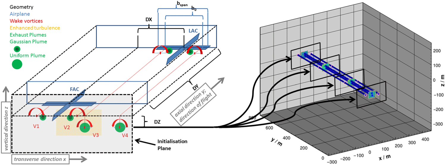
Throughout the paper, the transverse (cross-stream) direction is along x, the flight (stream-wise or axial) direction along y, and the vertical direction along z, as illustrated in Fig. 1.
The following subsection shortly describes EULAG-LCM, whereas a MGLET-description is deferred to the appendix.
2.1 LES model EULAG with Lagrangian ice microphysics LCM
The base model EULAG(Reference Smolarkiewicz, Margolin, Lin, Laprise and Ritchie41,Reference Prusa, Smolarkiewicz and Wyszogrodzki42) solves the Navier-Stokes (NS) momentum and energy equations. In its current version, various approximations of the NS equations can be dealt with, ranging from a Boussinesq, an anelastic, a pseudo-incompressible to a compressible version(Reference Smolarkiewicz, KÜhnlein and Wedi43). It relies on the iterative upwind scheme MPDATA (Multidimensional Positive Definite Advection Transport Algorithm(Reference Smolarkiewicz and Margolin44)) with substantially reduced implicit diffusion compared to the classical upwind scheme. The transport algorithm belongs to the class of NFT (non-oscillatory forward-in-time scheme) and is at least of second order. EULAG is an all-scale model with atmospheric applications ranging from global(Reference Smolarkiewicz, Margolin and Wyszogrodzki45), mesoscale(Reference Kurowski, Grabowski and Smolarkiewicz46) to local(Reference Smolarkiewicz, Sharman, Weil, Perry, Heist and Bowker47) scale optionally featuring dynamic grid deformation(Reference Prusa and Smolarkiewicz48) and adaptive moving meshes(Reference KÜhnlein, Smolarkiewicz and Dörnbrack49). Sub-grid turbulence modelling is based on a classical TKE approach(Reference Margolin, Smolarkiewicz and Sorbjan50,Reference Schumann51) . Domain decomposition in all three spatial directions allows perfect scalability in massive parallel applications with  $O(10^4)$
processors(Reference Piotrowski, Wyszogrodzki and Smolarkiewicz52). In the present study, we use the anelastic formulation, a time-constant uniform Cartesian grid, and 2D horizontal domain decomposition with
$O(10^4)$
processors(Reference Piotrowski, Wyszogrodzki and Smolarkiewicz52). In the present study, we use the anelastic formulation, a time-constant uniform Cartesian grid, and 2D horizontal domain decomposition with  $32 \times 6$
processors. The EULAG solution procedure, the underlying equation set and numerical parameter choices used here are summarised in Section 2.1 of Unterstrasser et al.(Reference Unterstrasser, Paoli, Sölch, Kühnlein and Gerz35).
$32 \times 6$
processors. The EULAG solution procedure, the underlying equation set and numerical parameter choices used here are summarised in Section 2.1 of Unterstrasser et al.(Reference Unterstrasser, Paoli, Sölch, Kühnlein and Gerz35).
Fully coupled to the dynamical solver is the Lagrangian ice microphysics model LCM(Reference Sölch and Kärcher53,Reference Unterstrasser and Sölch54) , which comprises explicit aerosol and ice microphysics for simulating pure ice clouds like natural cirrus(Reference Sölch and Kärcher55) or contrails(Reference Unterstrasser and Sölch56,Reference Unterstrasser, Gierens, Sölch and Lainer57) . In the Lagrangian approach, ice crystals are represented by simulation particles (SIPs) that are advected by the fluid. Each SIP represents a certain number of (identical) real crystals and stores information, e.g. on the discrete position  $\mathbf{x}_{SIP}$
, the mass
$\mathbf{x}_{SIP}$
, the mass  $m_{SIP}$
and the habit of the ice crystals that are bundled in a SIP. In its full version, microphysics-related processes on the simulation particles include homogeneous freezing of liquid supercooled aerosol particles, heterogeneous ice nucleation, deposition growth of ice crystals, sedimentation, aggregation, latent heat release and radiative impact on particle growth. For the given problem, it is not necessary to use the full LCM apparatus. As in previous EULAG-LCM studies of the early contrail evolution(Reference Unterstrasser1,Reference Unterstrasser and Görsch2) , deposition growth (including a Kelvin correction term) and latent heat release are the only microphysical processes switched on.
$m_{SIP}$
and the habit of the ice crystals that are bundled in a SIP. In its full version, microphysics-related processes on the simulation particles include homogeneous freezing of liquid supercooled aerosol particles, heterogeneous ice nucleation, deposition growth of ice crystals, sedimentation, aggregation, latent heat release and radiative impact on particle growth. For the given problem, it is not necessary to use the full LCM apparatus. As in previous EULAG-LCM studies of the early contrail evolution(Reference Unterstrasser1,Reference Unterstrasser and Görsch2) , deposition growth (including a Kelvin correction term) and latent heat release are the only microphysical processes switched on.
LCM uses information of the velocity and thermodynamic variables as provided by EULAG. A second order Runge-Kutta scheme is used to solve the advection equation for each SIP
 \begin{equation} \dot{\mathbf{x}}_{SIP} = \mathbf{u}_{SIP}, \end{equation}
where the particle velocity  $\mathbf{u}_{SIP}$
is a superposition of the fluid velocity
$\mathbf{u}_{SIP}$
is a superposition of the fluid velocity  $\mathbf{u}_{LES}$
, an auto-correlated turbulent contribution
$\mathbf{u}_{LES}$
, an auto-correlated turbulent contribution  $\mathbf{u}_{SGS}$
, which is based on the TKE-value provided by EULAG and accounts for SGS motions, and lastly the terminal settling velocity
$\mathbf{u}_{SGS}$
, which is based on the TKE-value provided by EULAG and accounts for SGS motions, and lastly the terminal settling velocity  $w_{sed}$
in the vertical direction (as written above, sedimentation is not relevant in the present problem and
$w_{sed}$
in the vertical direction (as written above, sedimentation is not relevant in the present problem and  $w_{sed}$
is set to zero).
$w_{sed}$
is set to zero).
Microphysical processes are computed for each SIP, e.g. the ice crystal deposition growth is a function of temperature, water vapour and ice crystal properties
 \begin{equation} \dot{m}_{SIP} = f_{DEP}(m_{SIP}, T_{LES}(\mathbf{x}_{SIP}), qv_{LES}(\mathbf{x}_{SIP}), ...). \end{equation}
Summing up  $\dot{m}_{SIP}$
of all SIPs in a grid box, one can derive the rate of change of the water vapour concentration qv, which appears as source term in the EULAG prognostic equation of
$\dot{m}_{SIP}$
of all SIPs in a grid box, one can derive the rate of change of the water vapour concentration qv, which appears as source term in the EULAG prognostic equation of  $qv_{LES}$
. Similarly, latent heating as derived in LCM is accounted for in the EULAG temperature equation.
$qv_{LES}$
. Similarly, latent heating as derived in LCM is accounted for in the EULAG temperature equation.
From the SIP data, Eulerian representations of, e.g. ice crystal number concentration N can be derived a-posteriori. Moreover, those 3D fields can be integrated along one or two spatial dimensions in order to obtain transverse/vertical profiles of ice crystal number ( $\mathcal{N}_{t}$
and
$\mathcal{N}_{t}$
and  $\mathcal{N}_{v}$
) or the total ice crystal number per meter of flight path (
$\mathcal{N}_{v}$
) or the total ice crystal number per meter of flight path ( $\mathcal{N}$
). Note that the derived quantities are averages along flight direction. Following U2014, we use the following definitions:
$\mathcal{N}$
). Note that the derived quantities are averages along flight direction. Following U2014, we use the following definitions:
 \begin{align} \mathcal{N}(t) & =\frac{1}{L_{y}}{\int\int\int} N(x,y,z,t) dx\: dy\: dz\: \end{align}
 \begin{align} \mathcal{N}_{v}(z) & = \frac{1}{L_{y}} \int_{0}^{Lx}\int_{0}^{Ly} N(x,y,z)\: dx dy, \end{align}
 \begin{align} \mathcal{N}_{t}(x) & = \frac{1}{L_{y}} \int_{0}^{Lz}\int_{0}^{Ly} N(x,y,z)\: dz dy , \end{align}
EULAG-LCM simulations were run at the HPC cluster of DKRZ Hamburg. Typically, the massively parallel computations use 192 cores and run for 25h consuming around 5,000 CPUh.
2.2 Model setup
2.2.1 Basic parameters
We perform temporal LES assuming homogeneous flow conditions along flight direction. In our previous wake vortex studies, the initial flow field consisted of a background turbulent field (produced by an a-priori simulation with specified turbulence level and stratification) and a pair of counter-rotating Lamb-Oseen vortices. Here, a four-vortex system is superimposed on the background field and describes the flow state downstream of the follower aircraft (FAC). This initialisation plane can be seen in the left part of Fig. 1. The vortices of the FAC are labelled  $V_{1}$
and
$V_{1}$
and  $V_{2}$
, and the ones of the leader aircraft (LAC)
$V_{2}$
, and the ones of the leader aircraft (LAC)  $V_{3}$
and
$V_{3}$
and  $V_{4}$
. We will refer to
$V_{4}$
. We will refer to  $V_{2}$
and
$V_{2}$
and  $V_{3}$
as inner vortices (IV) and to
$V_{3}$
as inner vortices (IV) and to  $V_{1}$
and
$V_{1}$
and  $V_{4}$
as outer vortices (OV). The idealised 2D flow field of the initialisation plane is uniformly initialised at each slice of the simulation domain as indicated in the right part of the figure. We note that the black boxes are only used for illustration purposes and the actual 2D flow field is prescribed over a larger cross-section than suggested by the black boxes.
$V_{4}$
as outer vortices (OV). The idealised 2D flow field of the initialisation plane is uniformly initialised at each slice of the simulation domain as indicated in the right part of the figure. We note that the black boxes are only used for illustration purposes and the actual 2D flow field is prescribed over a larger cross-section than suggested by the black boxes.
For the sake of simplicity, we study a formation flight scenario with two identical aircraft. We use two aircraft of type A350 or B777 with a wing span of  $b_s=60.9$
m and a mass which would generate wake vortices with circulation
$b_s=60.9$
m and a mass which would generate wake vortices with circulation  $\Gamma_{t=0}=520$
m2/s. The separation distance between the vortices is
$\Gamma_{t=0}=520$
m2/s. The separation distance between the vortices is  $b_{0}=(\pi/4)\, b_s=47.3\textrm{m}$
.
$b_{0}=(\pi/4)\, b_s=47.3\textrm{m}$
.
In a first simplistic and clearly unrealistic approach, each vortex  $V_i$
is initialised with
$V_i$
is initialised with  $|\Gamma_i|=\Gamma_{t=0}$
. A vortex core radius of
$|\Gamma_i|=\Gamma_{t=0}$
. A vortex core radius of  $r_{c}=4\textrm{m}$
is prescribed. We will refine the flow field initialisation in Section 2.2.2.
$r_{c}=4\textrm{m}$
is prescribed. We will refine the flow field initialisation in Section 2.2.2.
Figure 1 sketches the geometry of the formation flight scenario. The two AC have a stream-wise separation DY (along flight direction) and span-wise (lateral) separation DX. In commercial applications the extended formation flight with stream-wise separations of  $N_y=20$
to 40 wing spans is the preferred pattern and corresponds to a time separation of 5–10s (simply given by
$N_y=20$
to 40 wing spans is the preferred pattern and corresponds to a time separation of 5–10s (simply given by  $\Delta t_{LAC/FAC}= N_y b_s/U$
, where U is the AC speed). Due to safety reasons, shorter separations are foreseen only in the military sector. Upon the passage of the FAC, the vortex pair of the LAC descends. In the plane of initialisation, which is downstream of FAC and illustrated by the shaded area in Fig. 1, the separation DY along flight direction is translated into a vertical displacement DZ of the LAC vortex pair (
$\Delta t_{LAC/FAC}= N_y b_s/U$
, where U is the AC speed). Due to safety reasons, shorter separations are foreseen only in the military sector. Upon the passage of the FAC, the vortex pair of the LAC descends. In the plane of initialisation, which is downstream of FAC and illustrated by the shaded area in Fig. 1, the separation DY along flight direction is translated into a vertical displacement DZ of the LAC vortex pair ( $DZ=w_{0} \Delta t_{LAC/FAC}$
, where
$DZ=w_{0} \Delta t_{LAC/FAC}$
, where  $w_{0}=(2 \Gamma_{0})/(\pi^2 b_s)$
is the descent speed of the vortex pair). A lateral (span-wise) separation DX of around 0.8 wing spans was found to give optimal fuel benefits in previous studies and is used in this study as a default. The red blobs indicate the relative position of the four vortex centres (VC) and the arrows show the sense of rotation.
$w_{0}=(2 \Gamma_{0})/(\pi^2 b_s)$
is the descent speed of the vortex pair). A lateral (span-wise) separation DX of around 0.8 wing spans was found to give optimal fuel benefits in previous studies and is used in this study as a default. The red blobs indicate the relative position of the four vortex centres (VC) and the arrows show the sense of rotation.
The temperature at cruise altitude is  $T^*= 217\textrm{K}$
, the relative humidity with respect to ice is everywhere
$T^*= 217\textrm{K}$
, the relative humidity with respect to ice is everywhere  $RH_{i}^*=110\%$
, the Brunt-Väisälä frequency is
$RH_{i}^*=110\%$
, the Brunt-Väisälä frequency is  $N_{BV}=1.15\cdot 10^{-2}/\text{s}$
and the eddy dissipation rate is
$N_{BV}=1.15\cdot 10^{-2}/\text{s}$
and the eddy dissipation rate is  $\epsilon = 10^{-7}\text{m}^2\:/ {\rm {s}}^{3}$
. The pressure at the bottom of the domain is 250hPa. EULAG simulations use the anelastic approximation and a stable background temperature profile is prescribed according to
$\epsilon = 10^{-7}\text{m}^2\:/ {\rm {s}}^{3}$
. The pressure at the bottom of the domain is 250hPa. EULAG simulations use the anelastic approximation and a stable background temperature profile is prescribed according to  $N_{BV}$
. MGLET uses the Boussinesq approximation and we prescribe
$N_{BV}$
. MGLET uses the Boussinesq approximation and we prescribe  $\theta_{0}=330\textrm{K}$
and
$\theta_{0}=330\textrm{K}$
and  $d\:\theta_s / dz = 4.46$
K/km. The ambient conditions represent typical conditions of the upper troposphere and have been chosen in analogy to Unterstrasser(Reference Unterstrasser1) (abbr. from now on as U2014). Note that unlike to the lower atmosphere, where cloud formation is initiated at water vapour saturation, the formation of ice clouds in the upper troposphere is inhibited and substantial supersaturation is required for ice nucleation to proceed. This makes ice supersaturation and
$d\:\theta_s / dz = 4.46$
K/km. The ambient conditions represent typical conditions of the upper troposphere and have been chosen in analogy to Unterstrasser(Reference Unterstrasser1) (abbr. from now on as U2014). Note that unlike to the lower atmosphere, where cloud formation is initiated at water vapour saturation, the formation of ice clouds in the upper troposphere is inhibited and substantial supersaturation is required for ice nucleation to proceed. This makes ice supersaturation and  $RH_{i}$
-values
$RH_{i}$
-values  $> 100\%$
a common phenomenon of the upper troposphere. Contrail ice formation occurs in the expanding exhaust jets and is not bound to ambient
$> 100\%$
a common phenomenon of the upper troposphere. Contrail ice formation occurs in the expanding exhaust jets and is not bound to ambient  $RH_{i}$
. By the way, this gives also the explanation for skies that are crowded by contrails in an otherwise cloud-free scenario.
$RH_{i}$
. By the way, this gives also the explanation for skies that are crowded by contrails in an otherwise cloud-free scenario.
Finally, we summarise contrail-related aspects of the initialisation, which are similar to the A350/B777-setup of Unterstrasser and Görsch(Reference Unterstrasser and Görsch2) (abbr. from now on as UG2014). The green discs in Fig. 1 show the positions of the exhaust plumes. At the time of initialisation, the plumes of the LAC are assumed to be fully entrained into the wake vortices and discs with uniform concentrations are collocated with the VCs (default setup of UG2014). For the FAC plumes, Gaussian plumes are initialised inboard of the VCs (setup as in Section 3.4 of UG2014, a more detailed description of this setup type is given in U2014). The initial ice mass and crystal number per meter of flight path are  $\mathcal{I}_{0} = 3.0\cdot 10^{-2}$
kg/m and
$\mathcal{I}_{0} = 3.0\cdot 10^{-2}$
kg/m and  $\mathcal{N}_{0} = 6.8\cdot 10^{12}/\text{m}$
(total of both AC). This corresponds to an ‘emission’ index
$\mathcal{N}_{0} = 6.8\cdot 10^{12}/\text{m}$
(total of both AC). This corresponds to an ‘emission’ index  $EI_{iceno} = 2.8\cdot 10^{14}$
per kg of burned fuel. Each plume carries one fourth of all ice crystals. Overall, around
$EI_{iceno} = 2.8\cdot 10^{14}$
per kg of burned fuel. Each plume carries one fourth of all ice crystals. Overall, around  $82 \cdot 10^{6}$
Lagrangian particles are used to represent the ice crystals. As in preceding studies the initial ice crystal sizes are log-normally distributed with width
$82 \cdot 10^{6}$
Lagrangian particles are used to represent the ice crystals. As in preceding studies the initial ice crystal sizes are log-normally distributed with width  $r_{SD}=3.0$
(details, see Section 2.2 of U2014).
$r_{SD}=3.0$
(details, see Section 2.2 of U2014).
The model domain has dimensions  $L_{x}=768\text{m},\ L_{y}=132\text{m}$
and
$L_{x}=768\text{m},\ L_{y}=132\text{m}$
and  $L_{z}=600\text{m}$
. The cruise altitude of the two AC is at
$L_{z}=600\text{m}$
. The cruise altitude of the two AC is at  $z=350\textrm{m}$
. Periodic boundary conditions are applied in the horizontal and rigid boundaries in the vertical. In several plots the z-coordinate will be shifted to identify the cruise altitude with
$z=350\textrm{m}$
. Periodic boundary conditions are applied in the horizontal and rigid boundaries in the vertical. In several plots the z-coordinate will be shifted to identify the cruise altitude with  $z=0\textrm{m}$
. Moreover, the x-coordinate will be shifted such that the body of the (left) FAC is aligned with
$z=0\textrm{m}$
. Moreover, the x-coordinate will be shifted such that the body of the (left) FAC is aligned with  $x=0$
. Figure 1 illustrates the domain size (yet for a grid sensitivity simulation with
$x=0$
. Figure 1 illustrates the domain size (yet for a grid sensitivity simulation with  $L_{y}=792\text{m}$
) and the coordinate system.
$L_{y}=792\text{m}$
) and the coordinate system.
All basic parameters are summarised in Table 1.
Default numerical, atmospheric, aircraft formation flight and ice crystal parameters of the simulations

2.2.2 Inner vortices
So far, we assumed that the two IVs are not disturbed and  $\Gamma_{2}=-\Gamma_{3}=\Gamma_{t=0}$
. The fuel saving of the FAC results from the fact that it receives lift from the IV of the LAC. The lift loading is not equally distributed across the two wings of the FAC and
$\Gamma_{2}=-\Gamma_{3}=\Gamma_{t=0}$
. The fuel saving of the FAC results from the fact that it receives lift from the IV of the LAC. The lift loading is not equally distributed across the two wings of the FAC and  $|\Gamma_{2}| < |\Gamma_{1}|$
(Reference Kless, Aftosmis, Andrew Ning and Nemec15). Moreover, the roll-up process of
$|\Gamma_{2}| < |\Gamma_{1}|$
(Reference Kless, Aftosmis, Andrew Ning and Nemec15). Moreover, the roll-up process of  $V_{2}$
is affected by the close-by LAC IV
$V_{2}$
is affected by the close-by LAC IV  $V_{3}$
. On the other hand, also the evolution of the LAC IV
$V_{3}$
. On the other hand, also the evolution of the LAC IV  $V_{3}$
is disturbed as the vortex or certain areas of it impinge on the FAC wing. Such interactions between a solid body and a stream-wise oriented vortex have been simulated recently. A series of studies analysed the flow field a few chords downstream of a rigid flat plate wing with a specified angle-of-attack and results were found to depend sensitively on the lateral and vertical offset of the incident vortex relative to the wing(Reference Garmann and Visbal58,Reference Barnes, Visbal and Huang59) . Barnes et al.(Reference Barnes, Visbal and Gordnier60) considered a flexible wing including aeroelastic effects. The experimental study of Inasawa et al.(Reference Inasawa, Mori and Asai61) addresses the vortex impingement on a trailing wing by visualising the flow field with PIV (particle image velocimetry). They found that the circulation of the emerging wing tip vortex of the trailing wing can be higher or lower compared to the default case without an impinging vortex, depending on the relative position of the impinging vortex. All of the mentioned impingement studies use a setup resembling close formation flight; probably because the smaller domain of interest compared to extended flight scenarios requires less expensive numerical simulations or leads to smaller experiment dimensions in the wind channel. On the other hand, the findings may be generalised to extended FF scenarios as the properties of the lead vortex do not change too much between a few wing spans (once the roll-up is completed) and 30 wing spans behind the aircraft. However, those studies do not provide information whether or not the flow of the LAC IV
$V_{3}$
is disturbed as the vortex or certain areas of it impinge on the FAC wing. Such interactions between a solid body and a stream-wise oriented vortex have been simulated recently. A series of studies analysed the flow field a few chords downstream of a rigid flat plate wing with a specified angle-of-attack and results were found to depend sensitively on the lateral and vertical offset of the incident vortex relative to the wing(Reference Garmann and Visbal58,Reference Barnes, Visbal and Huang59) . Barnes et al.(Reference Barnes, Visbal and Gordnier60) considered a flexible wing including aeroelastic effects. The experimental study of Inasawa et al.(Reference Inasawa, Mori and Asai61) addresses the vortex impingement on a trailing wing by visualising the flow field with PIV (particle image velocimetry). They found that the circulation of the emerging wing tip vortex of the trailing wing can be higher or lower compared to the default case without an impinging vortex, depending on the relative position of the impinging vortex. All of the mentioned impingement studies use a setup resembling close formation flight; probably because the smaller domain of interest compared to extended flight scenarios requires less expensive numerical simulations or leads to smaller experiment dimensions in the wind channel. On the other hand, the findings may be generalised to extended FF scenarios as the properties of the lead vortex do not change too much between a few wing spans (once the roll-up is completed) and 30 wing spans behind the aircraft. However, those studies do not provide information whether or not the flow of the LAC IV  $V_{3}$
is also disturbed far from the centre and whether or not the roll-up of the FAC IV
$V_{3}$
is also disturbed far from the centre and whether or not the roll-up of the FAC IV  $V_{2}$
is such that a potential vortex is a good approximation for the flow field at large radii.
$V_{2}$
is such that a potential vortex is a good approximation for the flow field at large radii.
All in all, this leads to the situation that the flow field initialisation has some highly uncertain aspects.
Radial profiles of tangential velocity (left), vorticity (middle) and circulation (right) for a potential vortex (black dotted), a Lamb-Oseen vortex (black solid), and a weakened Lamb-Oseen (red solid:  $\textit{R}_{\textit{weak}}\,=\, \text{15}\textrm{m}$
; red dashed:
$\textit{R}_{\textit{weak}}\,=\, \text{15}\textrm{m}$
; red dashed:  $\textit{R}_{\textit{weak}} \,=\, \text{25}\textrm{m}$
). The core radius
$\textit{R}_{\textit{weak}} \,=\, \text{25}\textrm{m}$
). The core radius  $\textit{r}_{\textit{c}} \,=\, \text{4}\text{m}$
and the total circulation
$\textit{r}_{\textit{c}} \,=\, \text{4}\text{m}$
and the total circulation  $\Gamma_{\textit{tot}} \,=\,\\ \Gamma_{\text{0}} \,=\, \text{520}$
m2/s.
$\Gamma_{\textit{tot}} \,=\,\\ \Gamma_{\text{0}} \,=\, \text{520}$
m2/s.

In our default setup, we leave the two OVs  $V_{1}$
and
$V_{1}$
and  $V_{4}$
as is (using a standard Lamb-Oseen radial profile of tangential velocity
$V_{4}$
as is (using a standard Lamb-Oseen radial profile of tangential velocity  $u_\theta$
) and damp the two IVs. For radii
$u_\theta$
) and damp the two IVs. For radii  $r < R_{weak}$
,
$r < R_{weak}$
,  $u_\theta$
is multiplied by a scaling factor that increases linearly from 0.2 at
$u_\theta$
is multiplied by a scaling factor that increases linearly from 0.2 at  $r=0$
to 1 at
$r=0$
to 1 at  $r = R_{weak}$
. The modified profile
$r = R_{weak}$
. The modified profile  $u_\theta(r)$
together with the standard profile is plotted in Fig. 2(a). The consequences on the radial distributions of vorticity
$u_\theta(r)$
together with the standard profile is plotted in Fig. 2(a). The consequences on the radial distributions of vorticity  $\omega_y(r)$
and circulation
$\omega_y(r)$
and circulation  $\Gamma(r)$
are illustrated in panels (b) and (c).
$\Gamma(r)$
are illustrated in panels (b) and (c).
Based on observations by McKenna et al.(Reference McKenna, Bross and Rockwell62) we introduce additional turbulent velocity fluctuations (white noise fluctuations with root mean square velocity  $u_{rms,ET}=2\:$
m/s) in a rectangular box encompassing the two IVs (see yellow box in Fig. 1). The box is
$u_{rms,ET}=2\:$
m/s) in a rectangular box encompassing the two IVs (see yellow box in Fig. 1). The box is  $L_{x,ET}=DX$
broad and the lateral boundaries are aligned with the centres of the AC bodies. The vertical boundaries are
$L_{x,ET}=DX$
broad and the lateral boundaries are aligned with the centres of the AC bodies. The vertical boundaries are  $15\textrm{m}$
above the centre of
$15\textrm{m}$
above the centre of  $V_{2}$
and
$V_{2}$
and  $15\textrm{m}$
below the centre of
$15\textrm{m}$
below the centre of  $V_{3}$
giving a box height of
$V_{3}$
giving a box height of  $L_{z,ET}= DZ+30\textrm{m}$
.
$L_{z,ET}= DZ+30\textrm{m}$
.
Keeping in mind the uncertainties of the IV initialisation, several options are tested in an extended sensitivity experiment. In one simulation, both IVs are damped over a larger area by increasing  $R_{weak}$
from
$R_{weak}$
from  $15\textrm{}$
to
$15\textrm{}$
to  $25\textrm{m}$
; see the red dashed lines in Fig. 2 for the impact on the vortex properties. The overly simplistic approach outlined in Section 2.2.1 can be referred to as simulation with
$25\textrm{m}$
; see the red dashed lines in Fig. 2 for the impact on the vortex properties. The overly simplistic approach outlined in Section 2.2.1 can be referred to as simulation with  $R_{weak}=0\textrm{m}$
. The centres of the two IVs are around
$R_{weak}=0\textrm{m}$
. The centres of the two IVs are around  $15\textrm{m}$
apart from each other. Hence, a variation of
$15\textrm{m}$
apart from each other. Hence, a variation of  $R_{weak}$
substantially affects the interference among the IVs.
$R_{weak}$
substantially affects the interference among the IVs.
In further tests, the vortex strength is reduced not only locally around the core region, but globally for all radii. This means that the circulation values  $|\Gamma_{2}|$
and
$|\Gamma_{2}|$
and  $|\Gamma_{3}|$
are decreased. In such cases with ‘full’ damping, the damping is uniform across the whole radius range and no additional local damping is introduced (i.e.
$|\Gamma_{3}|$
are decreased. In such cases with ‘full’ damping, the damping is uniform across the whole radius range and no additional local damping is introduced (i.e.  $R_{weak}=0\textrm{m}$
). In one simulation, both IVs are similarly weakened by setting
$R_{weak}=0\textrm{m}$
). In one simulation, both IVs are similarly weakened by setting  $\Gamma_{2}=-\Gamma_{3}= 0.5\: \Gamma_{t=0}$
. In another simulation, an unsymmetrical damping with
$\Gamma_{2}=-\Gamma_{3}= 0.5\: \Gamma_{t=0}$
. In another simulation, an unsymmetrical damping with  $\Gamma_{2}= 0.6\: \Gamma_{t=0}$
and
$\Gamma_{2}= 0.6\: \Gamma_{t=0}$
and  $\Gamma_{3}= -0.4\: \Gamma_{t=0}$
is prescribed. This assumes that the destruction of or energy drain from the LAC vortex
$\Gamma_{3}= -0.4\: \Gamma_{t=0}$
is prescribed. This assumes that the destruction of or energy drain from the LAC vortex  $V_{3}$
is stronger than the potential beneficial reduction of the induced drag at the FAC, which is linked to generation of a weaker vortex
$V_{3}$
is stronger than the potential beneficial reduction of the induced drag at the FAC, which is linked to generation of a weaker vortex  $V_{2}$
. In the full damping cases, not only the mutual interference is affected, also the effect of the IVs on the two OVs is modified. Finally, in another sensitivity simulation with default
$V_{2}$
. In the full damping cases, not only the mutual interference is affected, also the effect of the IVs on the two OVs is modified. Finally, in another sensitivity simulation with default  $R_{weak}=15\textrm{m}$
, local turbulence is not enhanced.
$R_{weak}=15\textrm{m}$
, local turbulence is not enhanced.
All sensitivity simulations concerned with the IV initialisation are listed in blocks 4 to 6 of the ‘Sensitivity experiments’ Section of Table 2. The sensitivity to the IV initialisation will be reported in Section 6.1.
Parameter variations of the sensitivity simulations

2.3 Sensitivity experiments
Besides sensitivity tests accounting for the uncertainties of the IV initialisation discussed in the latter section, several physical parameters are varied. In real flight, it will not be operationally feasible to keep the lateral and vertical offset fixed over time, in particular the transverse shift has to consider the effect of cross winds. To account for these uncertainties, DX takes values of  $45,\ 55$
and
$45,\ 55$
and  $60\textrm{m}$
in a simulation series, complementing the default value of
$60\textrm{m}$
in a simulation series, complementing the default value of  $50\textrm{m}$
. Moreover, DZ is reduced to 0 or
$50\textrm{m}$
. Moreover, DZ is reduced to 0 or  $7\textrm{m}$
or enlarged to
$7\textrm{m}$
or enlarged to  $25\textrm{m}$
(default
$25\textrm{m}$
(default  $14\textrm{m}$
). A dominant parameter for the contrail evolution is the ambient relative humidity
$14\textrm{m}$
). A dominant parameter for the contrail evolution is the ambient relative humidity  $RH_{i}$
, which is varied from 100% to 140% similar to previous studies. A list of all sensitivity simulations is given in Table 2. We note that the default values are framed by a box and that in each sensitivity simulation only a single parameter is varied.
$RH_{i}$
, which is varied from 100% to 140% similar to previous studies. A list of all sensitivity simulations is given in Table 2. We note that the default values are framed by a box and that in each sensitivity simulation only a single parameter is varied.
3.0 RESULTS
The results section starts with a short presentation of an example simulation. This is followed by a detailed analysis of how the four vortices interact with each other and how they move. Finally, the implications on plume dimensions and contrail properties are discussed and differences to the classical single aircraft case are highlighted.
3D contour plot of vorticity magnitude at six different times. The times and the plotted contour surface level (in units: per s) are given in each panel. The various panels use different scales and the black box depicts a cube with length  $\text{50}\text{m}$
. Moreover, contours are shown in several slices along flight direction (four slices in the top row and two in the bottom row, the constant colour bar is shown only in the top right panel).
$\text{50}\text{m}$
. Moreover, contours are shown in several slices along flight direction (four slices in the top row and two in the bottom row, the constant colour bar is shown only in the top right panel).

3.1 Example simulation
In this paragraph we shortly describe the flow/vortex evolution of an example simulation over several minutes. For this, Fig. 3 displays 3D contour plots of vorticity magnitude (the time and the contour surface level are indicated in each panel). We choose the default simulation, yet for illustration purposes with an enlarged domain length along flight direction ( $L_y=792\textrm{m}$
instead of 132m, the simulation is listed in the last row of Table 2). In the first panel at
$L_y=792\textrm{m}$
instead of 132m, the simulation is listed in the last row of Table 2). In the first panel at  $t=2$
s, the four vortex tubes are straight and the relative positions between them reflect the geometric initialisation as outlined before in Fig. 1. Moreover, coloured contours are plotted in four slices perpendicular to the flight direction. Those reveal the enhanced turbulence that was superimposed in a rectangular box around the two IVs during the initialisation. The panel for
$t=2$
s, the four vortex tubes are straight and the relative positions between them reflect the geometric initialisation as outlined before in Fig. 1. Moreover, coloured contours are plotted in four slices perpendicular to the flight direction. Those reveal the enhanced turbulence that was superimposed in a rectangular box around the two IVs during the initialisation. The panel for  $t=16$
s shows that secondary vorticity structures (SVSs) have emerged around the two IVs. Moreover, those two vortices move towards the right OV. Section 3.2 will explain in detail the reasons for this lateral propagation. Soon after, the right OV
$t=16$
s shows that secondary vorticity structures (SVSs) have emerged around the two IVs. Moreover, those two vortices move towards the right OV. Section 3.2 will explain in detail the reasons for this lateral propagation. Soon after, the right OV  $V_{4}$
(as labelled in Fig. 1) captures
$V_{4}$
(as labelled in Fig. 1) captures  $V_{3}$
. Those two now form a vortex pair and move away from the other IV
$V_{3}$
. Those two now form a vortex pair and move away from the other IV  $V_{2}$
. After 60s, the vortex pair
$V_{2}$
. After 60s, the vortex pair  $V_{3} \& V_{4}$
effectively moved upwards, many SVSs shape up around them and high vorticity values are not any longer confined to two concentrated tubes (as is obvious from the contour slice in front). On the other hand, the vortices
$V_{3} \& V_{4}$
effectively moved upwards, many SVSs shape up around them and high vorticity values are not any longer confined to two concentrated tubes (as is obvious from the contour slice in front). On the other hand, the vortices  $V_{1}$
and
$V_{1}$
and  $V_{2}$
still feature straight vortex tubes. A closer inspection shows that vortex
$V_{2}$
still feature straight vortex tubes. A closer inspection shows that vortex  $V_{1}$
is stronger than
$V_{1}$
is stronger than  $V_{2}$
, as the red area with vorticity magnitude
$V_{2}$
, as the red area with vorticity magnitude  $\omega > 1.5$
/s is larger. Moreover, a small-amplitude small-wavelength meandering of
$\omega > 1.5$
/s is larger. Moreover, a small-amplitude small-wavelength meandering of  $V_{2}$
is apparent. After 3min, the vortex pair
$V_{2}$
is apparent. After 3min, the vortex pair  $V_{3} \& V_{4}$
has dissolved and only a few patches with elevated
$V_{3} \& V_{4}$
has dissolved and only a few patches with elevated  $\omega$
-values occur. Contrarily, the two other vortices can be still tracked as they still feature fairly straight vortex tubes and only weak SVSs are present. After 5min, the weaker
$\omega$
-values occur. Contrarily, the two other vortices can be still tracked as they still feature fairly straight vortex tubes and only weak SVSs are present. After 5min, the weaker  $V_{2}$
-vortex has dissolved and only
$V_{2}$
-vortex has dissolved and only  $V_{1}$
remains. Another 1.5min later at
$V_{1}$
remains. Another 1.5min later at  $t=6.5\min$
, mostly only irregular patterns of enhanced vorticity have survived. Most simulations are carried out until 10min, where we can safely assume that wake vortices induced dynamics has ceased.
$t=6.5\min$
, mostly only irregular patterns of enhanced vorticity have survived. Most simulations are carried out until 10min, where we can safely assume that wake vortices induced dynamics has ceased.
3.2 Tracking of the vortex centres
In the classical case of a single aircraft, a pair of counter-rotating vortices rolls up and the vortices mutually induce a downward movement at an initial speed of
 \begin{equation} w_{0}=\Gamma_{t=0}/(2\pi b_{0}). \end{equation}
At cruise conditions, the final vertical displacement and the decay of the vortices is mainly governed by the strength of thermal stratification e.g.(Reference Unterstrasser, Paoli, Sölch, Kühnlein and Gerz35,Reference Spalart63) and the well-known Crow-instability may occur(Reference Crow64). The formation flight simulations show a much more diverse behaviour and their early evolution is strongly affected by an interplay of the two close-by IVs. This will be demonstrated next by analysing the initial flow field; in particular, the velocity at the four VCs is analysed which gives a first hint of where each vortex travels in the beginning.
Figure 4 shows the initial positions of the four vortices (marked by asterisks) together with the velocities induced by the surrounding vortices at these positions (indicated by the arrows) for eight different cases. The arrows indicate the direction and strength of this velocity induction; the individual contributions of the vortices  $V_{1}$
(red),
$V_{1}$
(red),  $V_{4}$
(green) or the vortex dipole
$V_{4}$
(green) or the vortex dipole  $V_{2}/V_{3}$
(blue) and their combined effect (black) are depicted. The stream function of an ordinary vortex has circular contour lines and the arrows are tangentials. Hence, the green arrow originating from the red VC, e.g. is perpendicular to the line connecting the red VC with the green one. The contributions of the two IVs (blue arrows), which are counter-rotating, largely cancel out each other far from their centres. Hence, only their combined (and small) effect on the OVs
$V_{2}/V_{3}$
(blue) and their combined effect (black) are depicted. The stream function of an ordinary vortex has circular contour lines and the arrows are tangentials. Hence, the green arrow originating from the red VC, e.g. is perpendicular to the line connecting the red VC with the green one. The contributions of the two IVs (blue arrows), which are counter-rotating, largely cancel out each other far from their centres. Hence, only their combined (and small) effect on the OVs  $V_{1}$
and
$V_{1}$
and  $V_{4}$
is depicted. On the other hand, the blue arrows that originate from the IVs depict the velocity induction only from the adjacent IV (there is no self-induction). It follows that those blue arrows are perpendicular to the line connecting the two IVs.
$V_{4}$
is depicted. On the other hand, the blue arrows that originate from the IVs depict the velocity induction only from the adjacent IV (there is no self-induction). It follows that those blue arrows are perpendicular to the line connecting the two IVs.
Initial positions of the vortex centres (red asterisk:  $\textit{V}_{\text{1}}$
; blue asterisk:
$\textit{V}_{\text{1}}$
; blue asterisk:  $\textit{V}_{\text{2}}$
,
$\textit{V}_{\text{2}}$
,  $\textit{V}_{\text{3}}$
; green asterisk:
$\textit{V}_{\text{3}}$
; green asterisk:  $\textit{V}_{\text{4}}$
) and its approximate impact on the surrounding vortices. Each panel shows a different simulation (see title on top each panel). The arrows indicate the direction and strength of the velocity induction of the neighbouring vortices. The contribution of a specific vortex is plotted in the same colour as the asterisk labelling its centre. Note that the blue arrows originating from the OVs
$\textit{V}_{\text{4}}$
) and its approximate impact on the surrounding vortices. Each panel shows a different simulation (see title on top each panel). The arrows indicate the direction and strength of the velocity induction of the neighbouring vortices. The contribution of a specific vortex is plotted in the same colour as the asterisk labelling its centre. Note that the blue arrows originating from the OVs  $\textit{V}_{\text{1}}$
and
$\textit{V}_{\text{1}}$
and  $\textit{V}_{\text{4}}$
show the combined effect of both IVs
$\textit{V}_{\text{4}}$
show the combined effect of both IVs  $\textit{V}_{\text{2}}$
and
$\textit{V}_{\text{2}}$
and  $\textit{V}_{\text{3}}$
, whereas the blue arrows originating from
$\textit{V}_{\text{3}}$
, whereas the blue arrows originating from  $\textit{V}_{\text{2}}$
and
$\textit{V}_{\text{2}}$
and  $\textit{V}_{\text{3}}$
depict the velocity induction of the adjacent IV. At each vortex, the combined effect of all surrounding vortices is given by the black arrow. The lengths of the grey arrows inserted in each panel represent a wind speed of 2m/s. We use different scales for the
$\textit{V}_{\text{3}}$
depict the velocity induction of the adjacent IV. At each vortex, the combined effect of all surrounding vortices is given by the black arrow. The lengths of the grey arrows inserted in each panel represent a wind speed of 2m/s. We use different scales for the  $\textit{V}_{\text{1}}$
and
$\textit{V}_{\text{1}}$
and  $\textit{V}_{\text{4}}$
-arrows on the one hand and the
$\textit{V}_{\text{4}}$
-arrows on the one hand and the  $\textit{V}_{\text{2}}$
and
$\textit{V}_{\text{2}}$
and  $\textit{V}_{\text{3}}$
-arrows on the other hand reflecting the fact that the IVs move faster than the OVs.
$\textit{V}_{\text{3}}$
-arrows on the other hand reflecting the fact that the IVs move faster than the OVs.

The classical single aircraft case is introduced as a reference in panel (a). At both VCs, the velocity is given by  $u=(0,-w_{0})$
. With
$u=(0,-w_{0})$
. With  $\Gamma_{t=0}=520$
m2/s and
$\Gamma_{t=0}=520$
m2/s and  $b_{0}=47.3\textrm{m}$
(as in the formation flight scenarios),
$b_{0}=47.3\textrm{m}$
(as in the formation flight scenarios),  $w_{0}=1.75\textrm{m}/\textrm{s}$
follows.
$w_{0}=1.75\textrm{m}/\textrm{s}$
follows.
Moreover, the inserted legend introduces the angle  $\phi$
which defines the propagation direction.
$\phi$
which defines the propagation direction.
Panel (b) shows the default formation flight simulation. The velocity at the two OVs has a dominant downward component with a small lateral component to the right (black arrows). The downward transport is mainly induced by the other OV (green or red arrow, resp.). As noted before, the combined effect of the IVs on the OVs is rather small (blue arrows) and leads to a small counterclockwise rotation of the resulting velocities at  $V_{1}$
and
$V_{1}$
and  $V_{4}$
. Compared to the single aircraft case, the downward velocities are around a factor of two smaller, as the separation distance between the OVs (given by
$V_{4}$
. Compared to the single aircraft case, the downward velocities are around a factor of two smaller, as the separation distance between the OVs (given by  $b_{0} + DX$
) is roughly twice as large as in the single aircraft case (vortex separation
$b_{0} + DX$
) is roughly twice as large as in the single aircraft case (vortex separation  $b_{0}$
). The IVs are transported downward by both OVs. In sum, the downdraught is twice as large as in the single aircraft case. Yet, the strongest induction comes from the adjacent IV. The IVs mutually induce a strong transport to the right. In total, the IVs travel with more than
$b_{0}$
). The IVs are transported downward by both OVs. In sum, the downdraught is twice as large as in the single aircraft case. Yet, the strongest induction comes from the adjacent IV. The IVs mutually induce a strong transport to the right. In total, the IVs travel with more than  $5\textrm{m}\textrm{/s}$
in
$5\textrm{m}\textrm{/s}$
in  $\phi\approx 110^\circ$
direction. The second row shows scenarios with a smaller (panel c)) and larger (panel d)) lateral separation DX compared to the default scenario. We find similar velocity inductions at the OVs. Most notably, the mutual induction of the two IVs changes. In all cases, a strong lateral transport to the right remains. The vertical component, however, might be positive (for
$\phi\approx 110^\circ$
direction. The second row shows scenarios with a smaller (panel c)) and larger (panel d)) lateral separation DX compared to the default scenario. We find similar velocity inductions at the OVs. Most notably, the mutual induction of the two IVs changes. In all cases, a strong lateral transport to the right remains. The vertical component, however, might be positive (for  $DX > b_{0}$
) or negative (for
$DX > b_{0}$
) or negative (for  $DX < b_{0}$
). In total, we find an initial transport of the IVs at a speed of
$DX < b_{0}$
). In total, we find an initial transport of the IVs at a speed of  $6.5\textrm{m}/\textrm{s}$
in
$6.5\textrm{m}/\textrm{s}$
in  $\phi=135^\circ$
-direction for
$\phi=135^\circ$
-direction for  $DX=45\textrm{m}$
. For
$DX=45\textrm{m}$
. For  $DX=60\textrm{m}$
, the vertical velocities cancel out each other and the IVs travel purely horizontally with
$DX=60\textrm{m}$
, the vertical velocities cancel out each other and the IVs travel purely horizontally with  $u=3\textrm{m}/\textrm{s}$
. A change in the vertical offset DZ (third row) has similar effects as a DX-variation. Again, the mutual induction of the IVs is affected the most and changes their initial speed and direction. The two remaining cases in the fourth row will be discussed later. We can conclude that in all treated cases the early vortex evolution is characterised by a fast movement of the IVs towards the OV
$u=3\textrm{m}/\textrm{s}$
. A change in the vertical offset DZ (third row) has similar effects as a DX-variation. Again, the mutual induction of the IVs is affected the most and changes their initial speed and direction. The two remaining cases in the fourth row will be discussed later. We can conclude that in all treated cases the early vortex evolution is characterised by a fast movement of the IVs towards the OV  $V_{4}$
. In general, the movement is always towards the OV of the lower vortex pair, which is produced by the LAC.
$V_{4}$
. In general, the movement is always towards the OV of the lower vortex pair, which is produced by the LAC.
Contour plot of axial vorticity  $\omega_\textit{y}$
(averaged along the axial direction) for four different simulations (from top to bottom, see label on the right) and four times (from left to right, see time label inside each panel). The black and grey lines indicate the trajectories of the vortex centres (determined by local extrema of vorticity) from time
$\omega_\textit{y}$
(averaged along the axial direction) for four different simulations (from top to bottom, see label on the right) and four times (from left to right, see time label inside each panel). The black and grey lines indicate the trajectories of the vortex centres (determined by local extrema of vorticity) from time  $\textit{t} \,=\, \text{0}$
up to the displayed point in time. A sequence of symbols (see box in each panel) highlights the vortex positions every 30s, starting with a black plus sign for
$\textit{t} \,=\, \text{0}$
up to the displayed point in time. A sequence of symbols (see box in each panel) highlights the vortex positions every 30s, starting with a black plus sign for  $\textit{t} \,=\, \text{0}$
s.
$\textit{t} \,=\, \text{0}$
s.

Figure 5 shows the axial vorticity field averaged along flight direction at different vortex ages. The positions of the VCs are tracked by applying a simple vortex identification method based on finding local vorticity extrema.
Four simulations with different  $DX-DZ$
combinations are selected to demonstrate the diversity and complexity of possible vortex evolutions. The first row shows vorticity fields of the default simulation at
$DX-DZ$
combinations are selected to demonstrate the diversity and complexity of possible vortex evolutions. The first row shows vorticity fields of the default simulation at  $t=16\textrm{s},\ 1,\ 3$
and
$t=16\textrm{s},\ 1,\ 3$
and  $7.5\textrm{min}$
. In the beginning, both IVs approach
$7.5\textrm{min}$
. In the beginning, both IVs approach  $V_{4}$
. Soon,
$V_{4}$
. Soon,  $V_{3}$
gets closest to
$V_{3}$
gets closest to  $V_{4}$
and those two vortices feature a strong mutual induction. The
$V_{4}$
and those two vortices feature a strong mutual induction. The  $V_{3}\& V_{4}$
vortex pair moves quickly away;
$V_{3}\& V_{4}$
vortex pair moves quickly away;  $V_{3}$
propagates more than 300m in the first minute. The
$V_{3}$
propagates more than 300m in the first minute. The  $V_{3}$
,
$V_{3}$
, $V_{4}$
-trajectories bend upwards in counterclockwise fashion. After 1min both vortices are around
$V_{4}$
-trajectories bend upwards in counterclockwise fashion. After 1min both vortices are around  $50\textrm{m}$
above flight level, and more than
$50\textrm{m}$
above flight level, and more than  $60\textrm{m}$
above their creation level. Soon after, they slow down and seem to dissolve, at least our simple method based on longitudinally averaged vorticity evaluation is not able to identify them any longer. However, the 3D representation of vorticity in Fig. 3 has already revealed that the two vortices indeed have dissolved at that stage.
$60\textrm{m}$
above their creation level. Soon after, they slow down and seem to dissolve, at least our simple method based on longitudinally averaged vorticity evaluation is not able to identify them any longer. However, the 3D representation of vorticity in Fig. 3 has already revealed that the two vortices indeed have dissolved at that stage.
The vortices  $V_{1}\ V_{2}$
also form a pair and mutually induce a slow downward transport. After 3min, the vertical displacement of
$V_{1}\ V_{2}$
also form a pair and mutually induce a slow downward transport. After 3min, the vertical displacement of  $V_{1}$
and
$V_{1}$
and  $V_{2}$
is only
$V_{2}$
is only  $70\textrm{m}$
and 110m, respectively. Both vortices are long-living and, in particular,
$70\textrm{m}$
and 110m, respectively. Both vortices are long-living and, in particular,  $V_{1}$
can be tracked over 9min (the latest time shown here is 7.5min, though). Whereas
$V_{1}$
can be tracked over 9min (the latest time shown here is 7.5min, though). Whereas  $V_{2}$
more or less ceases to move and the VC resides around
$V_{2}$
more or less ceases to move and the VC resides around  $z=-100\textrm{m}$
, the direction of the
$z=-100\textrm{m}$
, the direction of the  $V_{1}$
-motion reverses at some point. Then
$V_{1}$
-motion reverses at some point. Then  $V_{1}$
starts to move upwards and eventually reaches its initial level
$V_{1}$
starts to move upwards and eventually reaches its initial level  $z=0\textrm{m}$
.
$z=0\textrm{m}$
.
The second row shows the simulation where DZ is raised from  $14\textrm{m}$
to
$14\textrm{m}$
to  $25\textrm{m}$
. The vorticity distribution after 16s looks similar to the latter case. The relative positions of the vortices
$25\textrm{m}$
. The vorticity distribution after 16s looks similar to the latter case. The relative positions of the vortices  $V_{2}$
,
$V_{2}$
,  $V_{3}$
and
$V_{3}$
and  $V_{4}$
are only slightly different. Again,
$V_{4}$
are only slightly different. Again,  $V_{3}$
and
$V_{3}$
and  $V_{4}$
build a vortex pair. However, the small initial differences qualitatively change its trajectory and the vortex pair travels sideways. After 1min,
$V_{4}$
build a vortex pair. However, the small initial differences qualitatively change its trajectory and the vortex pair travels sideways. After 1min,  $V_{3}$
is displaced by nearly 200m in lateral direction. Soon after, the motion slows down. After 4.5 min the vortex pair propagated only another 100m in lateral direction and moved slightly upwards. Eventually the vortices dissolve right above their creation level. As in the latter case, the vortices
$V_{3}$
is displaced by nearly 200m in lateral direction. Soon after, the motion slows down. After 4.5 min the vortex pair propagated only another 100m in lateral direction and moved slightly upwards. Eventually the vortices dissolve right above their creation level. As in the latter case, the vortices  $V_{1}\& V_{2}$
build a vortex pair and travel straight downward during the first 2min. Contrary, two the latter case, both vortices slow down, remain at around
$V_{1}\& V_{2}$
build a vortex pair and travel straight downward during the first 2min. Contrary, two the latter case, both vortices slow down, remain at around  $z=-100\textrm{m}$
and move slightly to the left.
$z=-100\textrm{m}$
and move slightly to the left.
The third row shows the simulation where the original DZ is retained and DX is increased by  $10\textrm{}$
to
$10\textrm{}$
to  $60\textrm{m}$
. The trajectories are qualitatively similar to case 2. Compared to this case, the final position of the
$60\textrm{m}$
. The trajectories are qualitatively similar to case 2. Compared to this case, the final position of the  $V_{3}\& V_{4}$
vortex pair is, however, only 200m to the right (instead of 300m in case 2) and around
$V_{3}\& V_{4}$
vortex pair is, however, only 200m to the right (instead of 300m in case 2) and around  $80\textrm{m}$
lower. Moreover, the
$80\textrm{m}$
lower. Moreover, the  $V_{1}\& V_{2}$
vortex pair travels further down and ends up
$V_{1}\& V_{2}$
vortex pair travels further down and ends up  $150{-}200\textrm{m}$
below the creation level.
$150{-}200\textrm{m}$
below the creation level.
The forth row shows a case with smaller DX ( $45\textrm{m}$
instead of
$45\textrm{m}$
instead of  $50\textrm{m}$
in case 1). Despite this small shift in lateral separation, the vortex evolution differs largely and features new aspects not seen in cases 1 to 3. At
$50\textrm{m}$
in case 1). Despite this small shift in lateral separation, the vortex evolution differs largely and features new aspects not seen in cases 1 to 3. At  $t=16$
s, the vortex
$t=16$
s, the vortex  $V_{2}$
is in between of
$V_{2}$
is in between of  $V_{3}$
and
$V_{3}$
and  $V_{4}$
.
$V_{4}$
.  $V_{2}$
and
$V_{2}$
and  $V_{4}$
have the same sense of rotation, the weaker vortex (
$V_{4}$
have the same sense of rotation, the weaker vortex ( $V_{2}$
) merges in a turbulent way into the strong vortex (
$V_{2}$
) merges in a turbulent way into the strong vortex ( $V_{4}$
), and
$V_{4}$
), and  $V_{2}$
cannot be tracked beyond
$V_{2}$
cannot be tracked beyond  $t=30$
s. Then,
$t=30$
s. Then,  $V_{3}$
spins around the strong vortex
$V_{3}$
spins around the strong vortex  $V_{4}$
in counterclockwise sense of rotation. After 70s, the
$V_{4}$
in counterclockwise sense of rotation. After 70s, the  $V_{3}$
trajectory completed a full cycle around
$V_{3}$
trajectory completed a full cycle around  $V_{4}$
and approaches
$V_{4}$
and approaches  $V_{1}$
.
$V_{1}$
.  $V_{1}$
and
$V_{1}$
and  $V_{3}$
have the same sense of rotation. And again, the weaker vortex (
$V_{3}$
have the same sense of rotation. And again, the weaker vortex ( $V_{3}$
) merges into the stronger vortex (
$V_{3}$
) merges into the stronger vortex ( $V_{1}$
) with the effect that
$V_{1}$
) with the effect that  $V_{3}$
can be tracked for less than 2min. After 2min, only
$V_{3}$
can be tracked for less than 2min. After 2min, only  $V_{1}$
and
$V_{1}$
and  $V_{4}$
are present at an altitude of around
$V_{4}$
are present at an altitude of around  $z=-100\textrm{m}$
. They continue to descend, though the descent slows down and comes basically to a halt after 3min. The final vertical displacement is less than 150m.
$z=-100\textrm{m}$
. They continue to descend, though the descent slows down and comes basically to a halt after 3min. The final vertical displacement is less than 150m.
The four simulations exhibit qualitatively different vortex evolutions despite their rather small ( $<10\textrm{m}$
) initial differences. To sum up: What are new aspects compared to the classical vortex descent behind a single aircraft?
$<10\textrm{m}$
) initial differences. To sum up: What are new aspects compared to the classical vortex descent behind a single aircraft?
We find a strong initial interaction of the two IVs and their lateral propagation (towards the OV of the lower vortex pair generated by the LAC). Afterwards, different phenomena can be observed in the various simulations: a strong lateral transport of the LAC vortex pair, its dissolution far above the flight level, a merging of co-rotating inner and outer vortices, or a reduced descent of the FAC vortex pair. In one case, a single vortex could be tracked over 9min, much longer than in the single aircraft case. Notably, the wake vortex evolution depends very sensitively on the initial lateral and vertical offset.
3.3 Plume dimensions
In this section, the spatial distribution of ice crystal number concentrations is analysed. Figure 6 juxtaposes the four FF simulations discussed before and the classical SA (single aircraft) case taken from U2014. For the moment, the ice crystals can be regarded as a passive tracer, i.e. changes in the contrail structure are only due to transport and not due to microphysical loss processes. Hence, we use the terms plume and exhaust instead of contrail and ice crystals in the following. We shortly recall the spatial plume initialisation. It consists of two circular discs with a uniform concentration field where the centres are collocated with the initial LAC VCs. The plumes of the FAC are given by Gaussian distributions. Their centres and peaks, respectively, are aligned with the lateral engine position and are inboard of the FAC VCs. The exhaust gets entrained into the nearby vortices within the first 10s see e.g. Fig. 33.2 in(Reference Unterstrasser, Sölch and Gierens65,Reference Paoli, Nybelen, Picot and Cariolle66) . Then, most of the exhaust is trapped inside the vortices and hence the plume expansion is roughly along the vortex trajectories. In the single aircraft case, the vortex descent leads to a substantial vertical plume expansion. In a thermally stable atmosphere, baroclinic instabilities occur around the vortices and exhaust is continuously detrained form the vortex system(Reference Holzäpfel, Hofbauer, Darracq, Moet, Garnier and Gago67). The detrained exhaust moves up again due to buoyancy and makes up a curtain between the actual and the initial vortex position(Reference Gerz and Holzäpfel68,Reference Gerz and Ehret69) . After 5min the highest plume concentrations can be found around the original emission altitude. Moreover, the lower part of the plume broadens between  $t=3$
and
$t=3$
and  $5\min$
since the vortex tubes start to meander along flight direction (over which is averaged here) as a result of the Crow instability(Reference Crow64). In this example, the plume is eventually 480m deep and 330m broad. After 5min the vortices have dissolved and the simulation ends (hence, no panel for
$5\min$
since the vortex tubes start to meander along flight direction (over which is averaged here) as a result of the Crow instability(Reference Crow64). In this example, the plume is eventually 480m deep and 330m broad. After 5min the vortices have dissolved and the simulation ends (hence, no panel for  $t=9\min$
exists for the single AC case). The further plume expansion is dominated by atmospheric processes and its analysis is not part of this study.
$t=9\min$
exists for the single AC case). The further plume expansion is dominated by atmospheric processes and its analysis is not part of this study.
Contour plot of ice crystal number concentrations (averaged along axial (=flight) direction) after 3, 5 and 9min. The simulations shown on columns 2–5 are the same as in Fig. 5 (see title on top). Additionally, the first column shows results from a single aircraft scenario adapted from Fig. 1 of(Reference Unterstrasser1), only for  $\textit{t} \,=\, \text{3}$
and 5min. For each point in time, the according colour bar is plotted on the right. To make the contrail dimensions of all panels visually comparable, all axes use the same scale. The two red values in each panel provide the contrail width and height (the thresholds used for their evaluation are smaller than the smallest contour level at display; hence the determined numerical values may be bigger than what the plot suggests). The FORMIC simulations use
$\textit{t} \,=\, \text{3}$
and 5min. For each point in time, the according colour bar is plotted on the right. To make the contrail dimensions of all panels visually comparable, all axes use the same scale. The two red values in each panel provide the contrail width and height (the thresholds used for their evaluation are smaller than the smallest contour level at display; hence the determined numerical values may be bigger than what the plot suggests). The FORMIC simulations use  $R{H_i} = {\mkern 1mu} {\rm{110}}\% $
, whereas the SA simulation uses
$R{H_i} = {\mkern 1mu} {\rm{110}}\% $
, whereas the SA simulation uses  $R{H_i} = {\mkern 1mu} {\rm{120}}\% $
.
$R{H_i} = {\mkern 1mu} {\rm{120}}\% $
.

In the FF scenarios, the vortices live longer and the third row shows the panels for  $t = 9\min$
. Moreover, all plot axes (including the single AC cases) use the same scale. From the different panel sizes used in the SA case on the one hand and FF cases on the other hand, it becomes directly apparent, that the plume dimensions are qualitatively different. For
$t = 9\min$
. Moreover, all plot axes (including the single AC cases) use the same scale. From the different panel sizes used in the SA case on the one hand and FF cases on the other hand, it becomes directly apparent, that the plume dimensions are qualitatively different. For  $t=3$
and
$t=3$
and  $5\min$
, the displayed FF plume structures in Fig. 6 are consistent with the vortex patterns found in Fig. 5. The vertical/lateral expansion is smaller/larger than in the SA case. After the vortices have dissolved and parts of the exhaust moved upwards due to buoyancy (
$5\min$
, the displayed FF plume structures in Fig. 6 are consistent with the vortex patterns found in Fig. 5. The vertical/lateral expansion is smaller/larger than in the SA case. After the vortices have dissolved and parts of the exhaust moved upwards due to buoyancy ( $t=9\min$
), the plumes are at most 280m deep (cf. to 480m in the SA case) and
$t=9\min$
), the plumes are at most 280m deep (cf. to 480m in the SA case) and  $500{-}700\textrm{m}$
broad (cf. to 330m in the SA case).
$500{-}700\textrm{m}$
broad (cf. to 330m in the SA case).
3.4 Sensitivity to lateral and vertical offset and relative humidity
Sections 3.2 and 3.3 discussed in detail several selected simulations. Contrarily, this section will give a systematic overview over all simulations and summarises physical sensitivities to the lateral offset DX, vertical offset DZ and relative humidity  $RH_{i}$
. Whereas DX and DZ strongly affect the vortex evolution (as seen before),
$RH_{i}$
. Whereas DX and DZ strongly affect the vortex evolution (as seen before),  $RH_{i}$
affects only ice microphysical processes in the contrail.
$RH_{i}$
affects only ice microphysical processes in the contrail.
The contrail structure is analysed by presenting profiles of ice crystal number in transverse and vertical direction. From this the contrail width and depth can be derived. The contrail depth, in particular, increases very quickly due to the wake vortex descent, much faster than by sedimentation or turbulent diffusion in later stages.
Figure 7 shows vertical profiles of ice crystal number for various values of DX (1st column), DZ (2nd column) and  $RH_{i}$
(3rd column) for three different instances of times (3, 5 and 7–8min). The discussion of the 4th column will be deferred to the appendix. The vertical profiles are computed by integrating ice crystal number concentrations over the transverse direction and averaging them along flight direction, ending up with units per m2. The area left of the curves is proportional to the total ice crystal number (units: per meter of flight path). The
$RH_{i}$
(3rd column) for three different instances of times (3, 5 and 7–8min). The discussion of the 4th column will be deferred to the appendix. The vertical profiles are computed by integrating ice crystal number concentrations over the transverse direction and averaging them along flight direction, ending up with units per m2. The area left of the curves is proportional to the total ice crystal number (units: per meter of flight path). The  $RH_{i}$
-column additionally shows vertical profiles of the classical SA case for the same range of
$RH_{i}$
-column additionally shows vertical profiles of the classical SA case for the same range of  $RH_{i}$
-values (simulation data taken from U2014).
$RH_{i}$
-values (simulation data taken from U2014). $\textit{DX}, \textit{DZ}, \textit{RH}_{\textit{i}}$
and IV sensitivity experiment: Profiles of ice crystal number for various times (indicated on the right of each row) in vertical direction. The simulation series are described in Table 2. The colours are defined in Fig. 9; the black solid curve in each column shows the same default simulation.
$\textit{DX}, \textit{DZ}, \textit{RH}_{\textit{i}}$
and IV sensitivity experiment: Profiles of ice crystal number for various times (indicated on the right of each row) in vertical direction. The simulation series are described in Table 2. The colours are defined in Fig. 9; the black solid curve in each column shows the same default simulation.

The most obvious aspect in the Fig. 7 is the difference between the FF scenarios on the one hand and the SA scenarios on the other hand. As already noted for the exemplary case in Fig. 6, the vortex pair in the single AC cases descends further down than the vortex system in the FF cases. After 3min, the SA plume extends from flight level down to 340m below flight level. In any FF scenario, the plume does not extend beyond 170m below flight level and much more ice crystals are present above flight altitude. After 5min, the SA plumes reach  $z=-400\textrm{m}$
and extend only moderately into regions above flight altitude, yielding a contrail vertical extent of 480m in the maximum case. In any FF scenario, no substantial further downward movement of the plumes is apparent and all plumes lie in the region between
$z=-400\textrm{m}$
and extend only moderately into regions above flight altitude, yielding a contrail vertical extent of 480m in the maximum case. In any FF scenario, no substantial further downward movement of the plumes is apparent and all plumes lie in the region between  $z=-190$
and 170m. The thickest contrail is about 300m thick and several thinner contrails are barely thicker than 200m.
$z=-190$
and 170m. The thickest contrail is about 300m thick and several thinner contrails are barely thicker than 200m.
The  $RH_{i}$
-column shows a strong
$RH_{i}$
-column shows a strong  $RH_{i}$
-effect on contrail ice crystal number which has been long known for the classical case(Reference Sussmann and Gierens31,Reference Lewellen and Lewellen33) . Downward moving air expands and heats adiabatically. Thereby the saturation vapour pressure increases, the local relative humidity decreases and leads to sublimation and loss of ice crystals. The weaker the ambient supersaturation (i.e. the closer
$RH_{i}$
-effect on contrail ice crystal number which has been long known for the classical case(Reference Sussmann and Gierens31,Reference Lewellen and Lewellen33) . Downward moving air expands and heats adiabatically. Thereby the saturation vapour pressure increases, the local relative humidity decreases and leads to sublimation and loss of ice crystals. The weaker the ambient supersaturation (i.e. the closer  $RH_{i}$
is at to 100%), the more ice crystals get lost during vortex descent. For the classical SA case, all ice crystals in the lower part of the plume vanish for
$RH_{i}$
is at to 100%), the more ice crystals get lost during vortex descent. For the classical SA case, all ice crystals in the lower part of the plume vanish for  $RH_{i} \le 110\%$
(red, green, black curves) and the contrail vertical dimension is reduced compared to the moister cases
$RH_{i} \le 110\%$
(red, green, black curves) and the contrail vertical dimension is reduced compared to the moister cases  $RH_{i}=120\%$
or 140% (blue and brown curve). In the FF scenarios, again fewer ice crystals survive, the lower the ambient
$RH_{i}=120\%$
or 140% (blue and brown curve). In the FF scenarios, again fewer ice crystals survive, the lower the ambient  $RH_{i}$
is. Yet, the
$RH_{i}$
is. Yet, the  $RH_{i}$
-effect is not as pronounced as in the SA cases and the contrail depth is about the same for all
$RH_{i}$
-effect is not as pronounced as in the SA cases and the contrail depth is about the same for all  $RH_{i}$
-values. This is due to the fact that the vertical plume displacement is less than in the SA case and the plume adiabatic heating is not as strong.
$RH_{i}$
-values. This is due to the fact that the vertical plume displacement is less than in the SA case and the plume adiabatic heating is not as strong. $\textit{DX}, \textit{DZ}, \textit{RH}_{\textit{i}}$
and IV sensitivity experiment: Profiles of ice crystal number for various times (indicated on the right of each row) in transverse direction. The simulation series are described in Table 2. The colours are defined in Fig. 9; the black solid curve in each column shows the same default simulation.
$\textit{DX}, \textit{DZ}, \textit{RH}_{\textit{i}}$
and IV sensitivity experiment: Profiles of ice crystal number for various times (indicated on the right of each row) in transverse direction. The simulation series are described in Table 2. The colours are defined in Fig. 9; the black solid curve in each column shows the same default simulation.

Next, we discuss the sensitivity to DX and DZ (1st and 2nd column). Unlike to  $RH_{i}$
, however, no systematic trends can be found in the sense that e.g. contrails become deeper for larger DX or DZ. For example, after 3min the contrail top varies from
$RH_{i}$
, however, no systematic trends can be found in the sense that e.g. contrails become deeper for larger DX or DZ. For example, after 3min the contrail top varies from  $z=0$
to
$z=0$
to  $z=150\textrm{m}$
among the four DX-simulations and from
$z=150\textrm{m}$
among the four DX-simulations and from  $z=50$
to
$z=50$
to  $z=150\textrm{m}$
among the four DZ-simulations. The contrail with the highest top (at
$z=150\textrm{m}$
among the four DZ-simulations. The contrail with the highest top (at  $z=150\textrm{m}$
) occurs for the intermediate values
$z=150\textrm{m}$
) occurs for the intermediate values  $DX=50\textrm{m}$
(out of the interval [
$DX=50\textrm{m}$
(out of the interval [ $45,60\textrm{m}$
]) and
$45,60\textrm{m}$
]) and  $DZ = 7\textrm{m}$
(out of the interval [
$DZ = 7\textrm{m}$
(out of the interval [ $0,25\textrm{m}$
]). Another example of non-systematic results can be seen in the DZ-panel for
$0,25\textrm{m}$
]). Another example of non-systematic results can be seen in the DZ-panel for  $t = 5\min$
. The vertical distributions for
$t = 5\min$
. The vertical distributions for  $DZ=0$
and
$DZ=0$
and  $25\textrm{m}$
are nearly the same. Moreover, the
$25\textrm{m}$
are nearly the same. Moreover, the  $DZ=14\textrm{m}$
-contrail has a similar vertical extent, yet with somewhat lower ice crystal numbers. The contrail with
$DZ=14\textrm{m}$
-contrail has a similar vertical extent, yet with somewhat lower ice crystal numbers. The contrail with  $DZ=7\textrm{m}$
differs qualitatively from the three other DZ-cases, as the contrail top is located around 100m higher. The vertical profiles after
$DZ=7\textrm{m}$
differs qualitatively from the three other DZ-cases, as the contrail top is located around 100m higher. The vertical profiles after  $7-8\min$
show that in all FF cases, the contrails are around 170 to 250m deep; the variation within the DX-series is even less than
$7-8\min$
show that in all FF cases, the contrails are around 170 to 250m deep; the variation within the DX-series is even less than  $30\textrm{m}$
. This small spread is remarkable as we have discussed and pinpointed the quite different vortex evolutions for small changes in DX or DZ.
$30\textrm{m}$
. This small spread is remarkable as we have discussed and pinpointed the quite different vortex evolutions for small changes in DX or DZ.
Next, transverse profiles for the same set of simulations are presented in Fig. 8. Again no trends with DX and DZ are apparent and we only report and shortly discuss results for  $t=5\text{min}$
and
$t=5\text{min}$
and  $t=7-8\text{min}$
. In the SA setup the single vortex pair has decayed after
$t=7-8\text{min}$
. In the SA setup the single vortex pair has decayed after  $<5$
min and simulations stop around
$<5$
min and simulations stop around  $t=5\min$
. Hence, the upper row of the figure enables the comparison between the FF and SA scenario, whereas the lower row reports the contrail dimensions after vortex decay for the FF scenarios. At initialisation, the FF contrails are around
$t=5\min$
. Hence, the upper row of the figure enables the comparison between the FF and SA scenario, whereas the lower row reports the contrail dimensions after vortex decay for the FF scenarios. At initialisation, the FF contrails are around  $130{-}140\textrm{m}$
(depending on DX) and SA contrails are around
$130{-}140\textrm{m}$
(depending on DX) and SA contrails are around  $90\textrm{m}$
broad. Within the first minute, a strong lateral transport occurs in some FF setups and the FF contrail width ranges from 200 to 320m (at
$90\textrm{m}$
broad. Within the first minute, a strong lateral transport occurs in some FF setups and the FF contrail width ranges from 200 to 320m (at  $t=1\min$
, not shown). Due to the different strength of the lateral transport in the individual FF cases, the transverse distribution differs strongly from case to case. We find distributions with one or two distinct peaks. The strongest peaks can occur at around
$t=1\min$
, not shown). Due to the different strength of the lateral transport in the individual FF cases, the transverse distribution differs strongly from case to case. We find distributions with one or two distinct peaks. The strongest peaks can occur at around  $x=0\textrm{m}$
in one case or at
$x=0\textrm{m}$
in one case or at  $x=300\textrm{m}$
in some other case. At
$x=300\textrm{m}$
in some other case. At  $t = 5\min$
, the contrail width varies from 350m for narrow FF contrails to 570m for the broadest FF contrail. A variation of
$t = 5\min$
, the contrail width varies from 350m for narrow FF contrails to 570m for the broadest FF contrail. A variation of  $RH_{i}$
changes the FF contrail width only weakly, whereas for the SA contrails the width ranges from 130 to 290m due to a Crow instability triggered vortex meandering in the lower plume part. Hence, typical SA contrails are usually not as broad as such behind a formation. FF contrails continue to spread after
$RH_{i}$
changes the FF contrail width only weakly, whereas for the SA contrails the width ranges from 130 to 290m due to a Crow instability triggered vortex meandering in the lower plume part. Hence, typical SA contrails are usually not as broad as such behind a formation. FF contrails continue to spread after  $t=5\min$
and for
$t=5\min$
and for  $t = 7 - 8 \min$
contrail width ranges from 400 to 680m.
$t = 7 - 8 \min$
contrail width ranges from 400 to 680m.
Integrating the vertical/transverse profiles over the vertical/transverse dimension gives the total ice crystal number  $\mathcal{N}$
per meter of flight path. Figure 9 shows the temporal evolution of the normalised total ice crystal number
$\mathcal{N}$
per meter of flight path. Figure 9 shows the temporal evolution of the normalised total ice crystal number  $f_\mathcal{N}(t)=\mathcal{N}(t)/\mathcal{N}(t=0)$
. Note that in the FF scenarios
$f_\mathcal{N}(t)=\mathcal{N}(t)/\mathcal{N}(t=0)$
. Note that in the FF scenarios  $\mathcal{N}(t=0)$
is twice as large as in the SA scenarios. The quantity
$\mathcal{N}(t=0)$
is twice as large as in the SA scenarios. The quantity  $f_\mathcal{N}$
diminishes over time due adiabatic heating induced ice crystal loss. The curves flatten out after several minutes indicating that the vortices stopped descending and pushing the local plume
$f_\mathcal{N}$
diminishes over time due adiabatic heating induced ice crystal loss. The curves flatten out after several minutes indicating that the vortices stopped descending and pushing the local plume  $RH_{i}$
below the saturation level. In the chosen classical SA case, this happens after 3 to 4min (the time of vortex break-up depends on the AC type and atmospheric stability, though, see UG2014). In some FF scenarios, the ice crystal loss gets negligible after around 6min. But in many cases crystal loss does not fully vanish and occurs over the complete simulation period, though at a reduced rate towards the end. Again no trends with DX and DZ can be observed and the fraction of surviving ice crystals
$RH_{i}$
below the saturation level. In the chosen classical SA case, this happens after 3 to 4min (the time of vortex break-up depends on the AC type and atmospheric stability, though, see UG2014). In some FF scenarios, the ice crystal loss gets negligible after around 6min. But in many cases crystal loss does not fully vanish and occurs over the complete simulation period, though at a reduced rate towards the end. Again no trends with DX and DZ can be observed and the fraction of surviving ice crystals  $f_{\mathcal{N},\text{s}}$
lies between 0.4 and 0.6 (surviving here refers to the
$f_{\mathcal{N},\text{s}}$
lies between 0.4 and 0.6 (surviving here refers to the  $f_\mathcal{N}$
-value at the end of the simulation).
$f_\mathcal{N}$
-value at the end of the simulation).  $RH_{i}$
is the dominant parameter for
$RH_{i}$
is the dominant parameter for  $f_{\mathcal{N},\text{s}}$
. Generally, a larger fraction of ice crystals survives in the FF than in the SA scenarios for a given
$f_{\mathcal{N},\text{s}}$
. Generally, a larger fraction of ice crystals survives in the FF than in the SA scenarios for a given  $RH_{i}$
-value. When
$RH_{i}$
-value. When  $RH_{i}$
is reduced from 140% to 120% and further down to 110%,
$RH_{i}$
is reduced from 140% to 120% and further down to 110%,  $f_{\mathcal{N},\text{s}}$
strongly decreases in the SA case (from 0.92 to 0.67 and further down to 0.28). In the FF scenarios, on the other hand, a reduction of
$f_{\mathcal{N},\text{s}}$
strongly decreases in the SA case (from 0.92 to 0.67 and further down to 0.28). In the FF scenarios, on the other hand, a reduction of  $RH_{i}=140\%$
down to 120% (the supersaturation
$RH_{i}=140\%$
down to 120% (the supersaturation  $RH_{i}-100\%$
is actually halved) has only a moderate effect and
$RH_{i}-100\%$
is actually halved) has only a moderate effect and  $f_{\mathcal{N},\text{s}}$
goes down from 0.96 to 0.89. For both
$f_{\mathcal{N},\text{s}}$
goes down from 0.96 to 0.89. For both  $RH_{i}$
-values, the vortex descent does not suffice to produce a substantial crystal loss. Only, a further reduction down to 110% makes the atmospheric buffer effect so small that the reduced vortex descent of FF cases produces local subsaturations that are sufficient to lead to a substantial loss of ice crystals (
$RH_{i}$
-values, the vortex descent does not suffice to produce a substantial crystal loss. Only, a further reduction down to 110% makes the atmospheric buffer effect so small that the reduced vortex descent of FF cases produces local subsaturations that are sufficient to lead to a substantial loss of ice crystals ( $f_{\mathcal{N},\text{s}}= 0.62$
).
$f_{\mathcal{N},\text{s}}= 0.62$
).
Temporal evolution of normalised ice crystal number  $\textit{f}_\mathcal{N}$
for the
$\textit{f}_\mathcal{N}$
for the  $\textit{DX}, \textit{DZ}, \textit{RH}_{\textit{i}}$
and IV sensitivity experiments. The simulation series are described in Table 2.
$\textit{DX}, \textit{DZ}, \textit{RH}_{\textit{i}}$
and IV sensitivity experiments. The simulation series are described in Table 2.

3.5 Robustness of findings
Various further experiments and a model comparison have been carried out in order to check the robustness of the above findings. These efforts are shortly summarised here and a full description is deferred to the appendix. In a grid sensitivity study, where the resolution and domain size along flight direction was varied, we find that the grid choices have a minor impact on the quantities of interest. Moreover, we perform four different realisations of the same simulation by simply shifting the turbulent background fields in lateral direction. We find small turbulence induced uncertainties implying the significance of the physically induced differences seen in the results section. Section 2.2.2 described various versions of IV initialisations. The initialisation choices have a non-negligible impact on the simulation results. Reducing this uncertainty will be an important future task and the way forward will be laid out in the discussion section. Finally, MGLET simulations are repeated for different DX-DZ combinations. In all three MGLET simulations we find patterns consistent with those of the EULAG simulations. Keeping in mind the diversity and complexity of the observed vortex evolution for small variations of DX or DZ, it is very convincing that the patterns are similar in both models and this boosts the confidence in the robustness of the simulation results.
4.0 DISCUSSION
In this section we discuss implications of the presented results.
Formation flight would probably reduce the frequency of potentially hazardous wake encounters at cruise levels for several reasons. The frequency of wake-vortex encounters increases with the square of air-traffic density(Reference Schumann and Sharman70). Organising the sky by routinely matching up several aircraft in a formation the flight routes of individual aircraft are not randomly distributed any longer and the effective air traffic density is reduced. Second, the present study demonstrated that, at least for two aircraft configurations, the descent speed and the final vertical displacement of the vortices in a FF scenario are smaller than in the classical SA scenario. Hence, the probability of interferences across different flight levels (the main reason for in-cruise wake vortex incidents(Reference Schumann and Sharman70-Reference Hoogstraten, Visser, Hart, Treve and Rooseleer72)) is likely to be reduced. Moreover, the experienced roll moments behind an AC formation wake may differ from those behind a single aircraft wake and may impact the severity of encounters. The latter aspect could be elaborated in a follow-up study based on the simulated flow fields. One aspect that may counteract those three effects is the fact that wake vortices appear to be more long living than in the single aircraft case.
Next, we discuss the implications of FF on long-living contrail-cirrus, which may persist for many hours(Reference Minnis, Young, Garber, Nguyen, Jr and Palikonda26) and have a substantial climate impact on global scale(Reference Bock and Burkhardt23). Regarding the long-term evolution over many hours, where sedimentation becomes important, the vertical expansion during the first several minutes can be viewed as a ‘sudden’ event. The spreading rate, i.e. the rate with which the contrail width increases with time, is proportional to vertical wind shear (which is an ubiquitous phenomenon in the upper troposphere) and to contrail depth. Moreover, sedimentation can be a limiting factor of contrail life time(Reference Bier, Burkhardt and Bock73). The fewer ice crystals are present initially in the contrail, the bigger they grow during contrail aging and the faster they fall out. Moreover, fewer, but larger ice crystals (with the same total ice mass) lead to an reduced extinction of shortwave radiation. For those reasons, the contrail vertical extent and the total ice crystal number after vortex decay are important quantities that can affect the contrail-cirrus properties over hours(Reference Lewellen25,Reference Unterstrasser and Gierens30) . UG2014, e.g. simulates contrails produced by various aircraft types and initial differences in ice crystal number and contrail depth lead to quantitative differences between the contrail-cirrus properties that remain over the total simulation period of 6h.
Earlier studies(Reference Unterstrasser and Sölch29) showed substantial saturation effects, when contrails were produced in close proximity and form a contrail-cluster. Compared to isolated contrails, the overall effect on radiation by an individual contrail in a cluster is smaller. Those as such contrails compete with neighbouring contrails for the available water vapour and hence their deposition growth is limited. In the formations studied here, two aircraft produce one ‘multi’-contrail. This case can be interpreted as the limiting case of the aforementioned contrail cluster simulation with initial contrail separation distances between 5 and 20km, as the distance of the two involved contrails tends to be much smaller here. So small even, that the distance is not well-defined any longer, as the contrails start to interact from the beginning of their existence. Hence, one can expect strong saturation effects in the case of formation flight simply due to the fact, that a single multi-contrail is produced by two AC. Without formation flight two independently produced contrails most likely occupy different air masses and can evolve undisturbed from each other.
The extent of saturation may be also affected by the fact, that a FF contrail contains more than twice as many ice crystals and is shallower than a single aircraft contrail. Contrail-cirrus simulations based on young FF and SA contrails will be presented in a follow-up study that investigates in more detail the climate benefit of formation flight due contrail modification.
As a last point of the discussion, a road map for reducing uncertainties associated with the inner vortex initialisation is outlined. In this study, temporal LES have been performed both with EULAG-LCM and MGLET, where a homogeneous vortex flow field together with periodic boundary conditions along flight direction is used. MGLET also features more advanced initialisation features, in particular for near ground wake vortex applications. A one-way coupling of RANS and LES simulations provides a methodology of simulating an aircraft flight through a computational domain, generating a wake in a realistic way(Reference Misaka, Holzäpfel and Gerz74,Reference Misaka, Holzäpfel and Gerz75) . For this purpose a pre-computed high-fidelity steady RANS flow field is swept through the LES domain. This is done to initialise the aircraft wake in the LES domain and is referred to as ‘spatial LES’. This method includes all stages of wake-vortex evolution, from roll-up to vortex decay and can capture, e.g. the touchdown manoeuvre and the wing in ground effect at varying vortex generation heights above the ground. The results have revealed valuable insights for cruise flight(Reference Misaka, Holzäpfel and Gerz75) as well as flight in ground proximity during the landing phase(Reference Stephan, Holzäpfel and Misaka76). However, the problems addressed in this work cannot be tackled with a one-way coupling, since it requires the following aircraft response on the wake of the leading aircraft. Therefore it is not applied here. Recently, a two-way RANS-LES coupling was developed, where a RANS code, simulating the aircraft flow, is coupled bidirectionally with the LES code MGLET. This allows simulating a realistic aircraft flight through a turbulent environment in a ground fixed domain. Having a leading and a following aircraft in that framework will provide a more realistic approach to formation flight, in particular valuable insight on the near field wake-vortex roll-up and early interaction can be obtained.
5.0 CONCLUSIONS
• For the first time, large-eddy simulations of the far field wake vortex evolution behind an aircraft formation have been performed, hereby focusing on a stratified atmosphere typical of cruise altitudes.
• The two LES models EULAG-LCM(Reference Smolarkiewicz, KÜhnlein and Wedi43,Reference Sölch and Kärcher53) and MGLET(Reference Manhart77) have been employed separately for such simulations. Both finite-difference codes have been used for wake vortex modelling in the recent past e.g.(Reference Unterstrasser1,Reference Unterstrasser and Görsch2,Reference Misaka, Holzäpfel, Hennemann, Gerz, Manhart and Schwertfirm36,Reference Stephan, Schrall and Holzäpfel38) . Moreover, the LES model core EULAG is fully coupled with the Lagrangian ice microphysics code LCM, which allows simulating the contrail evolution; in a reduced version LCM can be used for the Lagrangian transport of a passive tracer(Reference Unterstrasser, Paoli, Sölch, Kühnlein and Gerz35).
• Besides evaluating vorticity-related quantities and tracking of vortex centres, the present study investigates the aircraft plume dispersion which depends on and also reveals the wake vortex movement.
• For the sake of simplicity, we limited ourselves to scenarios of extended formation flight with two identical aircraft of type A350/B777. The simulations use an initialisation with two idealised wake vortex pairs and cover the full wake vortex life cycle up to 10min. Commonly, the span-wise separation of the two involved aircraft is around 80% of the wing span (determined in theory by the position of the so-called sweet spot) and hence the two inner vortices (i.e. the left vortex of the aircraft on the right hand side and right vortex of the aircraft on the left hand side) are the ones with the smallest separation and strongest mutual impact.
• Important physical initialisation parameters are given by the vertical and lateral separations of the two vortex pairs, which have been varied in the ranges
$DX\in [45,60\textrm{m}]$
and
$DZ\in [0,25\textrm{m}]$
. Both parameters in combination determine the relative position of the two inner vortices and where and how fast they propagate.• In the classical single aircraft case, the evolution of the wake vortices is characterised by their descent leading to a substantial plume/contrail expansion in vertical direction. In formation flight scenarios, wake vortex behaviour was found to be much more complex and also diverse. In the beginning, the two inner vortices always propagate towards the outer vortex of the lead aircraft. The exact propagation direction depends on the initial relative position of the inner vortices (i.e. on DX and DZ) and determines the further fate. Once the two inner vortices get close to the outer vortex, remarkably different things occur in the various simulations. In one simulation setup, it happened that the co-rotating inner vortex soon merges into the outer vortex. Later on, the two other vortices, both with the opposite sense of rotation, also merge. In several other simulations, on the other hand, the outer vortex forms a vortex pair with the counter-rotating inner vortex. Subsequently, this vortex pair tends to travel sideways or upwards. The two other vortices most often form a slowly descending long-living vortex pair which could be tracked for more than 5min. In one case, a vortex tube is still apparent after 7.5min and a single vortex can even be tracked over 9min. The wake vortices behind a single aircraft would have been fully dissolved after 5min in the same atmospheric environment.
• Even though the case-by-case variability of the wake vortex behaviour across the various formation flight scenarios is large, the final plume dimensions after vortex dissolution are in general characteristically different from those of single aircraft scenarios. The plumes are around 170 to 250m deep and 400 to 680m broad, whereas the same aircraft on a single mission would produce a 480m deep and 330m broad plume. Formation flight plumes are thus not as deep, yet they are broader.
• The robustness of the LES results treating such unprecedented formation flight scenarios is corroborated by a very good agreement between EULAG-LCM and MGLET simulations in terms of vortex evolution and plume dimensions.
• Notably,
$CO_{2}$
emissions are only one contribution to the aviation climate impact among several others like contrails and emission of water vapour and nitrogen oxides(Reference Sausen, Isaksen, Grewe, Hauglustaine, Lee, Myhre, Köhler, Pitari, Schumann and Stordal20,Reference Lee, Pitari, Grewe, Gierens, Penner, Petzold, Prather, Schumann, Bais, Berntsen, Iachetti, Lim and Sausen21) , where contrails probably have the largest radiative forcing(Reference Burkhardt and Kärcher22,Reference Bock and Burkhardt23) . All those components could be affected by formation flight. The (classical) early contrail evolution is characterised by vertical expansion due to vortex descent and by ice crystal loss. The latter is caused by adiabatic heating in the downward sinking primary wake, which leads to a local reduction of relative humidity and ice crystal sublimation.• With EULAG-LCM the early contrail evolution and its sensitivity to relative humidity over ice
$RH_{i}$
was investigated. We find that, compared to the classical case, fewer ice crystals are lost as the adiabatic heating is not as pronounced. Hence, the formation flight contrail contains more than twice as many ice crystals as the single aircraft contrail. Moreover, the contrails are shallower and broader which are a direct consequence of the wake vortex movements.• A follow-up numerical study that uses the present simulation data as input will focus on the contrail-cirrus evolution over several hours and assess the climate benefits by contrail saturation effects in formation flight scenarios.


ACKNOWLEDGEMENTS
The first author is partly funded by the BMWi LuFo project FORMIC (Formation Flight Impact on Climate). We thank T. Gerz for valuable comments on the manuscript. Computational resources for EULAG-LCM simulations were made available by the German Climate Computing Center (DKRZ) through support from the German Federal Ministry of Education and Research (BMBF) and for MGLET by the Gauss Center for Supercomputing/Leibniz Supercomputing Center under grant pr63zi.
APPENDIX
6.0 NUMERICAL CONSISTENCY
Whereas the results section focused on the impact of physical parameters, the appendix presents mostly numerical sensitivity tests and a model comparison in order to demonstrate the robustness of the presented results. The first subsection discusses the uncertainties associated with the uncertain initialisation of the two IVs. The second subsection investigates the sensitivity to grid parameters for the EULAG default simulation, whereas the third subsection highlights irreducible uncertainties associated with turbulence. The appendix concludes with a comparison of EULAG and MGLET results for three selected cases.
6.1 Uncertainties from the inner vortex initialisation
In Section 2.2.2 we described various versions of IV initialisations. The simulation results are presented in the right-most columns of Figs 7, 8 and 9. In the default case, the two IVs are damped in  $R_{weak}=15\textrm{m}$
-circles around the VC and turbulence is enhanced in a box around those two vortices (see yellow box in Fig.1). This simulation is shown in black (labelled by ‘15’ in the legend).
$R_{weak}=15\textrm{m}$
-circles around the VC and turbulence is enhanced in a box around those two vortices (see yellow box in Fig.1). This simulation is shown in black (labelled by ‘15’ in the legend).
In a first sensitivity test, we increased  $R_{weak}$
to
$R_{weak}$
to  $25\textrm{m}$
(label ‘25’). The bottom right panel of Fig. 4 illustrates how an increase of
$25\textrm{m}$
(label ‘25’). The bottom right panel of Fig. 4 illustrates how an increase of  $R_{weak}$
affects the initial flow field and propagation direction of each vortex. The induced velocities at the OVs are unaffected as their distance from the IVs is larger than
$R_{weak}$
affects the initial flow field and propagation direction of each vortex. The induced velocities at the OVs are unaffected as their distance from the IVs is larger than  $25\textrm{m}$
and IVs are not damped at that radii, irrespective of
$25\textrm{m}$
and IVs are not damped at that radii, irrespective of  $R_{weak}$
being 15 or
$R_{weak}$
being 15 or  $25\textrm{m}$
. The mutual induction of the IV is, however, reduced (see blue arrows). Together with the unchanged contribution of the OVs on the IVs, the propagation direction of the IV has a stronger downward and a weaker horizontal component (see black arrows).
$25\textrm{m}$
. The mutual induction of the IV is, however, reduced (see blue arrows). Together with the unchanged contribution of the OVs on the IVs, the propagation direction of the IV has a stronger downward and a weaker horizontal component (see black arrows).
We further tested two variants, where the vortex strength was reduced for all radii (i.e  $|\Gamma_{2}|$
and
$|\Gamma_{2}|$
and  $|\Gamma_{3}|$
are reduced), and not only locally close to the core as before. In one test, both vortices are similarly weakened (
$|\Gamma_{3}|$
are reduced), and not only locally close to the core as before. In one test, both vortices are similarly weakened ( $\Gamma_{2}=-\Gamma_{3}= 0.5\: \Gamma_{t=0}$
, label ‘5050’). In a second test, the reduction is unsymmetrical (
$\Gamma_{2}=-\Gamma_{3}= 0.5\: \Gamma_{t=0}$
, label ‘5050’). In a second test, the reduction is unsymmetrical ( $\Gamma_{2}= 0.6\: \Gamma_{t=0}$
and
$\Gamma_{2}= 0.6\: \Gamma_{t=0}$
and  $\Gamma_{3}= -0.4\: \Gamma_{t=0}$
, label ‘6040’). The bottom left panel of Fig. 4 shows again the immediate consequences on the initial vortex propagation. Unlike to the
$\Gamma_{3}= -0.4\: \Gamma_{t=0}$
, label ‘6040’). The bottom left panel of Fig. 4 shows again the immediate consequences on the initial vortex propagation. Unlike to the  $R_{weak}$
-change before, the full damping assumption also changes the propagation of the OVs. The IVs pull the OVs to right. If IV circulations are lowered, this effect is reduced and the OV propagation tends to become nearly purely vertical. The mutual induction of the IVs and their propagation is similar to the
$R_{weak}$
-change before, the full damping assumption also changes the propagation of the OVs. The IVs pull the OVs to right. If IV circulations are lowered, this effect is reduced and the OV propagation tends to become nearly purely vertical. The mutual induction of the IVs and their propagation is similar to the  $R_{weak}=25\textrm{m}$
-case.
$R_{weak}=25\textrm{m}$
-case.
Furthermore in yet another test (label ‘ET0’), turbulence was not enhanced. And last, we ran a simulation with the overly simplistic case with no damping at all, i.e. four identical vortices in the beginning (label ‘00’).
A simple observation from Figs 7, 8 and 9 is that the inclusion/omission of enhanced turbulence has a negligible impact on the vortex evolution, the spatial distribution of the ice crystals and ice crystal loss. Hence, the ET0-simulation will not be discussed any further in the following.
We recall the VC evolution of the default case as shown in Figs. 3 and 5. The IVs  $V_{2}$
and
$V_{2}$
and  $V_{3}$
move towards the right OV
$V_{3}$
move towards the right OV  $V_{4}$
.
$V_{4}$
.  $V_{4}$
picks up
$V_{4}$
picks up  $V_{3}$
and those two vortices form a vortex pair that decays quickly. Their trajectories are next to each other and bend upwards in a counterclockwise fashion.
$V_{3}$
and those two vortices form a vortex pair that decays quickly. Their trajectories are next to each other and bend upwards in a counterclockwise fashion.  $V_{1}$
and
$V_{1}$
and  $V_{2}$
also form a vortex pair that is slowly moving down and is more persistent than the other pair. In the various IV sensitivity studies, qualitative deviations from this rough pattern occur (not shown). In one simulation, e.g. the vortex
$V_{2}$
also form a vortex pair that is slowly moving down and is more persistent than the other pair. In the various IV sensitivity studies, qualitative deviations from this rough pattern occur (not shown). In one simulation, e.g. the vortex  $V_{2}$
remains longer under influence of
$V_{2}$
remains longer under influence of  $V_{4}$
and does not form a pair with
$V_{4}$
and does not form a pair with  $V_{1}$
. In another simulation, the co-rotating vortex
$V_{1}$
. In another simulation, the co-rotating vortex  $V_{2}$
merges into
$V_{2}$
merges into  $V_{4}$
at some point, the vortices
$V_{4}$
at some point, the vortices  $V_{1}$
and
$V_{1}$
and  $V_{4}$
form a persistent and slowly decaying vortex pair. The implications of those differences can be seen in the transverse and vertical ice crystal number profiles. The vertical profiles across the IV simulation series show some variation. The transverse profiles show a small spread (neglecting the out-lier simulation ‘00’) and non-zero ice crystal numbers are confined to the area
$V_{4}$
form a persistent and slowly decaying vortex pair. The implications of those differences can be seen in the transverse and vertical ice crystal number profiles. The vertical profiles across the IV simulation series show some variation. The transverse profiles show a small spread (neglecting the out-lier simulation ‘00’) and non-zero ice crystal numbers are confined to the area  $x=-200\textrm{m}$
to 250m. Also the extent of ice crystal loss depends on the IV initialisation. In the default case, around 60% of the ice crystals survive, whereas in most other IV simulations around 45% of the ice crystals survive. In general, it seems that the spread in the profiles is smaller across the IV series than across the DX- or DZ-series. Yet, the initialisation choices have a non-negligible impact on the simulation results. Reducing this uncertainty will be an important future task as detailed in the discussion section.
$x=-200\textrm{m}$
to 250m. Also the extent of ice crystal loss depends on the IV initialisation. In the default case, around 60% of the ice crystals survive, whereas in most other IV simulations around 45% of the ice crystals survive. In general, it seems that the spread in the profiles is smaller across the IV series than across the DX- or DZ-series. Yet, the initialisation choices have a non-negligible impact on the simulation results. Reducing this uncertainty will be an important future task as detailed in the discussion section.
6.2 Grid sensitivity
This section presents a grid sensitivity study for the default simulation ( $DX=50,\ DZ=14\textrm{m},\ RH_{i}=110\%$
). First, the vertical and lateral extent have to be chosen large enough to avoid interactions across the periodic lateral boundaries or with the rigid boundaries on the top/bottom. This was assured by choosing a fairly large domain with
$DX=50,\ DZ=14\textrm{m},\ RH_{i}=110\%$
). First, the vertical and lateral extent have to be chosen large enough to avoid interactions across the periodic lateral boundaries or with the rigid boundaries on the top/bottom. This was assured by choosing a fairly large domain with  $L_x=768\textrm{m}$
and
$L_x=768\textrm{m}$
and  $L_z=600\textrm{m}$
compared to previous classical wake vortex studies(Reference Misaka, Holzäpfel, Hennemann, Gerz, Manhart and Schwertfirm36) and similar to a study accounting for cross-wind effects(Reference Bricteux, Duponcheel, De Visscher and Winckelmans78). As in previous studies the grid boxes use
$L_z=600\textrm{m}$
compared to previous classical wake vortex studies(Reference Misaka, Holzäpfel, Hennemann, Gerz, Manhart and Schwertfirm36) and similar to a study accounting for cross-wind effects(Reference Bricteux, Duponcheel, De Visscher and Winckelmans78). As in previous studies the grid boxes use  $\Delta x = \Delta z = 1\textrm{m}$
. Along flight direction, the domain in classical wake vortex simulations is chosen such that one Crow modes can develop, i.e. around 400m for an AC with a wing span of
$\Delta x = \Delta z = 1\textrm{m}$
. Along flight direction, the domain in classical wake vortex simulations is chosen such that one Crow modes can develop, i.e. around 400m for an AC with a wing span of  $60\textrm{m}$
. Due to the strong interaction of the two IVs one cannot expect that a Crow mode with 400m long oscillations will occur in our FF simulations. Hence, we tested domains with various numbers of grid points
$60\textrm{m}$
. Due to the strong interaction of the two IVs one cannot expect that a Crow mode with 400m long oscillations will occur in our FF simulations. Hence, we tested domains with various numbers of grid points  $n_y=396,\ 198,\ 99$
and 66 and grid sizes
$n_y=396,\ 198,\ 99$
and 66 and grid sizes  $\Delta y= 2,\ 1$
and
$\Delta y= 2,\ 1$
and  $0.5\textrm{m}$
. The section grid parameters in Table 2 and the legend in Fig. 10 lists all six combinations of
$0.5\textrm{m}$
. The section grid parameters in Table 2 and the legend in Fig. 10 lists all six combinations of  $L_y=n_y \cdot \Delta y$
and
$L_y=n_y \cdot \Delta y$
and  $\Delta y$
that were tested. The largest simulation domain has a length of 792m and may contain a Crow oscillation of the OVs which have distance of around
$\Delta y$
that were tested. The largest simulation domain has a length of 792m and may contain a Crow oscillation of the OVs which have distance of around  $2 b_{0}$
or several Crow modes of two other vortices with a smaller separation.
$2 b_{0}$
or several Crow modes of two other vortices with a smaller separation.
Grid sensitivity experiment: Profiles of ice crystal number for various times (indicated on top of each column) in vertical (top row) and transverse (bottom row) direction. Six different combinations of ( $\textit{L}_\textit{y},\Delta \textit{y}$
) are shown (see legend and list in Table 2 (section grid parameters)).
$\textit{L}_\textit{y},\Delta \textit{y}$
) are shown (see legend and list in Table 2 (section grid parameters)).


Concerning the transverse distribution of ice crystal number, shown in the bottom row of Fig. 10, we find an excellent agreement among all six simulations. Also the vertical profiles shown in the top row match well in a qualitative sense, yet with increasing time the distributions of the various simulations differ moderately close to the contrail top. Moreover, no distinct oscillations along flight directions could be identified by inspecting longitudinal profiles (not shown). This finding is corroborated by the 3D vorticity fields in Fig. 3.
The negligible impact of the grid on the crystal loss mechanism and the total ice crystal evolution is exemplified in Fig. 11. All in all, we find that the choice of the grid has a minor effect on the quantities discussed in the results section. Hence, we decided to use the most inexpensive setting with  $L_y=132\textrm{m}$
and
$L_y=132\textrm{m}$
and  $\Delta y=2\textrm{m}$
which helped to keep the computational requirements in an acceptable range and allowed to perform several physical and numerical sensitivity studies.
$\Delta y=2\textrm{m}$
which helped to keep the computational requirements in an acceptable range and allowed to perform several physical and numerical sensitivity studies.
6.3 Turbulent realisation
In this sensitivity test, we use the default grid and also keep the default values of all other parameters unchanged. We perform four different realisations of the same simulation by simply shifting the turbulent background fields in lateral direction. Although the statistical turbulence properties are unchanged, the vortex system may evolve differently due to slightly different local interactions of the vortices and turbulence. The spread of the four simulations demonstrates the irreducible uncertainties associated with turbulence. If the simulation results of two simulations with different parameter settings (as presented in the results section) differ, those differences are only significant if they are larger than the spread given by the various realisations of a specific simulation. We find small turbulence induced uncertainties (Fig. 12 and right panel of Fig. 11) implying the significance of the physically induced differences seen in the results section.
Turbulent realisation experiment: Profiles of ice crystal number for various times (indicated on top of each column) in vertical (top row) and transverse (bottom row) direction. Four different realisations of the default simulation are shown. The black curve depicts the realisation of the default simulation that was used in many previous figures.

6.4 Comparison of EULAG-LCM and MGLET simulations
This section presents a comparison of EULAG-LCM and MGLET simulations.
The LES model MGLET, developed at the Technical University of Munich(Reference Manhart77), solves the incompressible NS equations. The kinematic viscosity is given as the sum of molecular viscosity  $\nu$
and eddy viscosity
$\nu$
and eddy viscosity  $\nu_t$
, determined by means of a Lagrangian dynamic sub-grid scale model(Reference Meneveau, Lund and Cabot79). The momentum equation and the continuity equation are solved by a finite-volume approach, using a fourth-order compact scheme by Hokpunna and Manhart(Reference Hokpunna and Manhart80). A split-interface algorithm is used for the parallel solution of the tri-diagonal system resulting from the compact scheme(Reference Hokpunna81). A third-order explicit Runge-Kutta method is used for the time integration. The simulations are performed in parallel, using a domain decomposition approach.
$\nu_t$
, determined by means of a Lagrangian dynamic sub-grid scale model(Reference Meneveau, Lund and Cabot79). The momentum equation and the continuity equation are solved by a finite-volume approach, using a fourth-order compact scheme by Hokpunna and Manhart(Reference Hokpunna and Manhart80). A split-interface algorithm is used for the parallel solution of the tri-diagonal system resulting from the compact scheme(Reference Hokpunna81). A third-order explicit Runge-Kutta method is used for the time integration. The simulations are performed in parallel, using a domain decomposition approach.
Contour plot of axial vorticity  $\omega_\textit{y}$
(averaged along the axial direction) analogous to Fig. 5, except that the last point in time (fourth column) and the simulation DX60 (third row) are not displayed. This figure shows MGLET simulation results instead of EULAG simulation results as in Fig. 5. See caption of that figure for more explanations.
$\omega_\textit{y}$
(averaged along the axial direction) analogous to Fig. 5, except that the last point in time (fourth column) and the simulation DX60 (third row) are not displayed. This figure shows MGLET simulation results instead of EULAG simulation results as in Fig. 5. See caption of that figure for more explanations.

Left column: Vortex positions from EULAG (solid, as shown in Fig. 5) and from MGLET (dotted, as shown in Fig. 13) for three setups (see label on the right). For a particular vortex, the trajectories of both models are shown as long as the vortex can be tracked in both models. Right column: Distance between the EULAG and MGLET vortex positions as a function of time. The different colours show the various vortices  $\textit{V}_{\textit{i}}$
(see legend in top-left panel).
$\textit{V}_{\textit{i}}$
(see legend in top-left panel).

MGLET uses the same turbulent background fields at initialisation as EULAG and superimposes the vortex fields in an identical way. EULAG uses Lagrangian particles with discrete positions for the representation of ice crystals and their advection. MGLET is not coupled to a ice microphysics module, but it offers the advection of a passive tracer represented by Eulerian field. Unlike to Lagrangian methods, Eulerian advection schemes do not perform well when strong gradients appear in the tracer distribution. Hence, in MGLET the plume initialisation with circles of uniform concentrations uses some smoothing in a transition layer. Due to operational constraints, MGLET simulations use a domain width of  $L_x=600\textrm{m}$
instead of 768m and the simulated time is 5min. Three of the four scenarios discussed in detail in Figs 5 and 6, namely the default simulation, the
$L_x=600\textrm{m}$
instead of 768m and the simulated time is 5min. Three of the four scenarios discussed in detail in Figs 5 and 6, namely the default simulation, the  $DZ=25\textrm{m}$
-simulation and the
$DZ=25\textrm{m}$
-simulation and the  $DX=45\textrm{m}$
-simulation, have been repeated with MGLET. Figure 13 depicts the vorticity distribution and tracks the movement of the VCs in the new simulations. The plot layout is analogous to the EULAG counterpart in Fig. 5, except that one simulation and the last point of time are discarded. In all three MGLET simulations we find patterns consistent with those of the EULAG simulations. In the default case, the
$DX=45\textrm{m}$
-simulation, have been repeated with MGLET. Figure 13 depicts the vorticity distribution and tracks the movement of the VCs in the new simulations. The plot layout is analogous to the EULAG counterpart in Fig. 5, except that one simulation and the last point of time are discarded. In all three MGLET simulations we find patterns consistent with those of the EULAG simulations. In the default case, the  $V_{3}$
,
$V_{3}$
, $V_{4}$
-trajectories bend upwards in counterclockwise fashion and the vortices
$V_{4}$
-trajectories bend upwards in counterclockwise fashion and the vortices  $V_{1}\& V_{2}$
form a pair with a slow downward transport as already seen in EULAG. In the
$V_{1}\& V_{2}$
form a pair with a slow downward transport as already seen in EULAG. In the  $DZ=25\textrm{m}$
-case, we again find a strong purely horizontal transport of the
$DZ=25\textrm{m}$
-case, we again find a strong purely horizontal transport of the  $V_{3}\& V_{4}$
vortex pair. And in the
$V_{3}\& V_{4}$
vortex pair. And in the  $DX=45\textrm{m}$
-case, we observe a merging of the co-rotating vortices
$DX=45\textrm{m}$
-case, we observe a merging of the co-rotating vortices  $V_{3}$
and
$V_{3}$
and  $V_{4}$
as in EULAG. Figure 14 overlays the vortex positions (left column) of EULAG (solid) and MGLET (dotted) and evaluate the distances between the EULAG and MGLET vortex positions (right column). The differences between the two models increase over time, but typically remain smaller than
$V_{4}$
as in EULAG. Figure 14 overlays the vortex positions (left column) of EULAG (solid) and MGLET (dotted) and evaluate the distances between the EULAG and MGLET vortex positions (right column). The differences between the two models increase over time, but typically remain smaller than  $50\textrm{m}$
after 5min for all four vortices. Keeping in mind the diversity and complexity of the observed vortex evolution for small variations of DX or DZ, it is very convincing that the patterns are similar in both models and this boosts the confidence in the robustness of the simulation results.
$50\textrm{m}$
after 5min for all four vortices. Keeping in mind the diversity and complexity of the observed vortex evolution for small variations of DX or DZ, it is very convincing that the patterns are similar in both models and this boosts the confidence in the robustness of the simulation results.
Tracer cross section similar to Fig. 6. Columns show the default, DZ25 and DX45 simulation. Times  $\textit{t} \,=\, \text{3}$
and 5min are shown.
$\textit{t} \,=\, \text{3}$
and 5min are shown.

Tracer vertical profiles of EULAG-LCM (1st and 3rd column) and MGLET (2nd and 4th column) simulations are juxtaposed. The colours of the default, DZ25 and DX45 simulation are black, blue and red, respectively. The black dotted curve shows EULAG-LCM simulation with  $\textit{RH}_{\textit{i}} \,=\, \text{140}\%$
.
$\textit{RH}_{\textit{i}} \,=\, \text{140}\%$
.

Figure 15 shows the MGLET passive tracer distribution similarly to the EULAG ice crystal number concentrations in Fig. 6. Since the vortex trajectories agreed well, it is not surprising that also the plume cross sections look similar. Again, the plume width and vertical extent are inserted in each panel. The given values mostly deviate less than  $50\textrm{m}$
from EULAG values. Considering the different advection treatment, the agreement is excellent. Finally, Fig. 17 juxtaposes transverse and vertical profiles of MGLET (right) and EULAG (left). As default,
$50\textrm{m}$
from EULAG values. Considering the different advection treatment, the agreement is excellent. Finally, Fig. 17 juxtaposes transverse and vertical profiles of MGLET (right) and EULAG (left). As default,  $RH_i = 110\%$
is used in the EULAG simulations. As a consequence, ice crystal loss occurs in all simulations of the DX and DZ sensitivity series and in particular in the three simulations discussed so far in this section. To clarify the effects of ice crystal loss, the EULAG result for
$RH_i = 110\%$
is used in the EULAG simulations. As a consequence, ice crystal loss occurs in all simulations of the DX and DZ sensitivity series and in particular in the three simulations discussed so far in this section. To clarify the effects of ice crystal loss, the EULAG result for  $RH_i=140\%$
(complementary to
$RH_i=140\%$
(complementary to  $RH_i=110\%$
as in the default case) is added to the plot (dotted black curve).
$RH_i=110\%$
as in the default case) is added to the plot (dotted black curve).
Tracer transverse profiles analogous to Fig. 16.


 Open access