


1. Introduction
The deposition of particles on the back side of a bluff body is an important problem in a wide range of applications, such as fouling of heat exchanger tubes (Li, Zhou & Cen Reference Li, Zhou and Cen2008; Weber et al. Reference Weber, Schaffel-Mancini, Mancini and Kupka2013; Kleinhans et al. Reference Kleinhans, Wieland, Frandsen and Spliethoff2018) and fouling of vehicles (Gaylard, Kirwan & Lockerby Reference Gaylard, Kirwan and Lockerby2018; Eidevåg et al. Reference Eidevåg, Eng, Kallin, Cesselgren, Bharadhwaj, Bangalore Narahari and Rasmuson2022). At the same time, this particular deposition process remains poorly understood. It is known that the back-side deposition efficiency on bluff bodies, such as cylinders, is much lower than that on the front side, but the spread in the available data is up to three orders of magnitude for the same flow conditions, as illustrated in figure 1 (Li et al. Reference Li, Zhou and Cen2008; Haugen & Kragset Reference Haugen and Kragset2010; Weber et al. Reference Weber, Schaffel-Mancini, Mancini and Kupka2013). In this study, we investigate particle deposition on the back side of a cylinder in the so-called shear-layer transition regime (Williamson Reference Williamson1996), where the flow in the wake is distinctively three-dimensional. More specifically, we investigate the Reynolds number range 1685–10 000, where the single-phase flow is amenable to direct numerical simulation (DNS). We track Lagrangian particles in the flow and analyse the back-side deposition events in an attempt to clarify the governing phenomena. Despite the industrial relevance and the current lack of understanding of the particle back-side deposition process, this is the first three-dimensional DNS with particle tracking to be performed for this canonical problem.
Back-side particle deposition efficiencies $\eta _{\textit{back}}$
as a function of the Stokes number on a circular cylinder in the range
$\eta _{\textit{back}}$
as a function of the Stokes number on a circular cylinder in the range $\textit{Re}=1065$
to
$\textit{Re}=1065$
to $\textit{Re}=28\,000$
(Li et al. Reference Li, Zhou and Cen2008; Haugen & Kragset Reference Haugen and Kragset2010; Weber et al. Reference Weber, Schaffel-Mancini, Mancini and Kupka2013).
$\textit{Re}=28\,000$
(Li et al. Reference Li, Zhou and Cen2008; Haugen & Kragset Reference Haugen and Kragset2010; Weber et al. Reference Weber, Schaffel-Mancini, Mancini and Kupka2013).

For the flow around a cylinder at the relevant Reynolds numbers, properties such as general wake behaviour, vortex-shedding frequencies and separation angles are well characterised in the literature, whereas there is a large scattering in the mean near-wake statistics (cf. Parnaudeau et al. Reference Parnaudeau, Carlier, Heitz and Lamballais2008). This spread has been attributed to the existence of a slow modulation of the wake size behind bluff bodies such as disks, spheres and cylinders (Berger, Scholz & Schumm Reference Berger, Scholz and Schumm1990; Rodriguez et al. Reference Rodriguez, Borell, Lehmkuhl, Segarra and Oliva2011; Lehmkuhl et al. Reference Lehmkuhl, Rodríguez, Borrell and Oliva2013). These modulations typically act on significantly longer time scales than vortex shedding, sometimes more than a factor 30 slower (Lehmkuhl et al. Reference Lehmkuhl, Rodríguez, Borrell and Oliva2013). The effect of such low-frequency phenomena on the back-side particle deposition is, however, not known, and hence their contribution to the scatter in figure 1 is also unknown.
This work aims to reveal the underlying mechanisms responsible for particle back-side deposition on a cylinder for Reynolds numbers in the range 1685–10 000. By fully resolving all scales of the fluid flow using DNS and by collecting particle statistics for more than 100 vortex-shedding periods, we are able to provide a comprehensive analysis of the back-side deposition process and its temporal variation. To the best of our knowledge, this is the first analysis of particle back-side deposition over such long periods of time so as to enable assessment of the role of low-frequency wake modulation. We first present the relevant equations and modelling assumptions in § 2. Then, § 3 presents the computational domain, modelling parameters and solvers used. The results for the time-dependent behaviour of the back-side deposition are given in § 4. Finally, § 5 summarises the main conclusions drawn from this work.
2. Theory
The DNS method used in this work directly solves the incompressible Navier–Stokes equations for the fluid flow. These equations are expressed in non-dimensional form as
 \begin{equation} \boldsymbol{\nabla }^*\boldsymbol{\cdot }\boldsymbol {u}_{\!f}^* = 0 \end{equation}
and
 \begin{equation} \frac {\partial \boldsymbol {u}_{\!f}^*}{\partial t^*} + (\boldsymbol {u}_{\!f}^* \boldsymbol{\cdot } \boldsymbol{\nabla }^*) \boldsymbol {u}_{\!f}^* = -\boldsymbol{\nabla }^*{p^*} + \frac {1}{\textit{Re}} {\nabla} ^{*2}{\boldsymbol {u}_{\!f}^*} , \end{equation}
where the asterisk represents non-dimensionalised quantities and operators. In the above equation, $\boldsymbol {u}_{\!f}^* = \boldsymbol {u}_{\!f}/U$
is fluid velocity,
$\boldsymbol {u}_{\!f}^* = \boldsymbol {u}_{\!f}/U$
is fluid velocity, $t^* = \textit{tU}/D$
is time,
$t^* = \textit{tU}/D$
is time, $p^* = p/(\rho _{\!f} U^2)$
is pressure,
$p^* = p/(\rho _{\!f} U^2)$
is pressure, $\rho _{\!f}$
is fluid density and
$\rho _{\!f}$
is fluid density and $\boldsymbol{\nabla }^* = D \boldsymbol{\nabla }$
is the nabla operator. The quantities have been normalised using the fluid free-stream velocity
$\boldsymbol{\nabla }^* = D \boldsymbol{\nabla }$
is the nabla operator. The quantities have been normalised using the fluid free-stream velocity $U$
and the diameter of the cylinder
$U$
and the diameter of the cylinder $D$
. The Reynolds number
$D$
. The Reynolds number $\textit{Re}$
is
$\textit{Re}$
is $\textit{Re} = \textit{UD} / \nu$
, where
$\textit{Re} = \textit{UD} / \nu$
, where $\nu = \mu /\rho _{\!f}$
is the kinematic viscosity and
$\nu = \mu /\rho _{\!f}$
is the kinematic viscosity and $\mu$
is the dynamic viscosity. Frequencies are reported in non-dimensional form using the Strouhal number,
$\mu$
is the dynamic viscosity. Frequencies are reported in non-dimensional form using the Strouhal number, $\textit{Str} = \textit{fD} / U$
, where
$\textit{Str} = \textit{fD} / U$
, where $f$
is the dimensional frequency.
$f$
is the dimensional frequency.
Particle trajectories are evolved using Lagrangian point-particle tracking, assuming that the particles are spherical and small in comparison with the relevant fluid flow scales. The particle positions and velocities are determined from Newton’s second law of motion:
 \begin{equation} \dfrac {\text{d} \boldsymbol {x}^*_{\!p}}{\text{d} t^*} = \boldsymbol {u}^*_{\!p} ,\end{equation}
 \begin{equation} m^* \dfrac {\text{d} \boldsymbol {u}^*_{\!p}}{\text{d} t^*} = \boldsymbol {F}^* \end{equation}
with particle position $\boldsymbol {x}^*_{\!p} = \boldsymbol {x}_{\!p} / D$
, particle velocity
$\boldsymbol {x}^*_{\!p} = \boldsymbol {x}_{\!p} / D$
, particle velocity $\boldsymbol {u}^*_{\!p} = \boldsymbol {u}_{\!p} / U$
, particle mass
$\boldsymbol {u}^*_{\!p} = \boldsymbol {u}_{\!p} / U$
, particle mass $m^* = m / (\rho _{\!f} D^3)$
and force from the fluid on the particle
$m^* = m / (\rho _{\!f} D^3)$
and force from the fluid on the particle $\boldsymbol {F}^* = \boldsymbol {F} / \rho _{\!f} D^2 U^2$
. It is assumed that the particle motion is determined by the drag force, such that
$\boldsymbol {F}^* = \boldsymbol {F} / \rho _{\!f} D^2 U^2$
. It is assumed that the particle motion is determined by the drag force, such that
 \begin{equation} \boldsymbol {F}^* = \frac {1}{2} C_{\!D} A^* \boldsymbol {u}_{\textit{rel}}^* |\boldsymbol {u}_{\textit{rel}}^*| \end{equation}
with drag coefficient $C_{\!D}$
, projected area of the particle
$C_{\!D}$
, projected area of the particle $A^* = \pi d_{\!p}^2/4 D^2$
, relative velocity between fluid and particle
$A^* = \pi d_{\!p}^2/4 D^2$
, relative velocity between fluid and particle $\boldsymbol {u}_{\textit{rel}}^* = (\boldsymbol {u}_{\!f} - \boldsymbol {u}_{\!p}) / U$
and particle diameter
$\boldsymbol {u}_{\textit{rel}}^* = (\boldsymbol {u}_{\!f} - \boldsymbol {u}_{\!p}) / U$
and particle diameter $d_{\!p}$
. The drag coefficient is determined as
$d_{\!p}$
. The drag coefficient is determined as
 \begin{equation} C_{\!D} = \frac {24}{\textit{Re}_{\!p}} \left ( 1 + \frac {1}{6} \textit{Re}_{\!p}^{2/3} \right ) \end{equation}
with particle Reynolds number $\textit{Re}_{\!p} = |\boldsymbol {u}_{\textit{rel}}| d_{\!p} / \nu$
.
$\textit{Re}_{\!p} = |\boldsymbol {u}_{\textit{rel}}| d_{\!p} / \nu$
.
The assumption that $\boldsymbol {F}^*$
can be determined from the drag force alone, as given by (2.5) and (2.6), implies that other effects (e.g. gravitational acceleration, buoyancy, unsteady drag (added mass and history effects), undisturbed fluid stresses, lift, Brownian motion and thermophoresis) are small in comparison with the steady drag. This is a good assumption for typical gas–solid flow scenarios involving small, spherical non-Brownian particles, where the particle-to-fluid density ratio is large and
$\boldsymbol {F}^*$
can be determined from the drag force alone, as given by (2.5) and (2.6), implies that other effects (e.g. gravitational acceleration, buoyancy, unsteady drag (added mass and history effects), undisturbed fluid stresses, lift, Brownian motion and thermophoresis) are small in comparison with the steady drag. This is a good assumption for typical gas–solid flow scenarios involving small, spherical non-Brownian particles, where the particle-to-fluid density ratio is large and $\textit{Re}_{\!p}$
is small (Bretherton Reference Bretherton1962; Morsi & Alexander Reference Morsi and Alexander1972; Maxey & Riley Reference Maxey and Riley1983; Haugen & Kragset Reference Haugen and Kragset2010; Michael et al. Reference Michael, Mark, Sasic and Ström2025). For the current problem,
$\textit{Re}_{\!p}$
is small (Bretherton Reference Bretherton1962; Morsi & Alexander Reference Morsi and Alexander1972; Maxey & Riley Reference Maxey and Riley1983; Haugen & Kragset Reference Haugen and Kragset2010; Michael et al. Reference Michael, Mark, Sasic and Ström2025). For the current problem, $\rho _{\!p} / \rho _{\!f}$
is set equal to
$\rho _{\!p} / \rho _{\!f}$
is set equal to $1000$
(
$1000$
( $\rho _{\!p}$
is the particle density) and the particle Reynolds number remains small. Even so, the drag correlation used (equation (2.6)) permits application beyond the Stokes flow regime, being valid until
$\rho _{\!p}$
is the particle density) and the particle Reynolds number remains small. Even so, the drag correlation used (equation (2.6)) permits application beyond the Stokes flow regime, being valid until $ \textit{Re}_p \lesssim 1000$
(Schiller Reference Schiller1933; Morsi & Alexander Reference Morsi and Alexander1972; Haugen & Kragset Reference Haugen and Kragset2010). Furthermore, we employ a one-way coupled approach in which the presence of particles does not influence the fluid and particles do not interact, neither hydrodynamically nor through collisions. The results are therefore limited to scenarios in which local particle concentrations do not exceed
$ \textit{Re}_p \lesssim 1000$
(Schiller Reference Schiller1933; Morsi & Alexander Reference Morsi and Alexander1972; Haugen & Kragset Reference Haugen and Kragset2010). Furthermore, we employ a one-way coupled approach in which the presence of particles does not influence the fluid and particles do not interact, neither hydrodynamically nor through collisions. The results are therefore limited to scenarios in which local particle concentrations do not exceed ${\simeq}\,10$
%. The current assumptions are well established in a wide range of industrially relevant applications involving particle deposition from a turbulent flow (Hansson et al. Reference Hansson, Lichtenegger, Pirker, Sasic and Ström2025).
${\simeq}\,10$
%. The current assumptions are well established in a wide range of industrially relevant applications involving particle deposition from a turbulent flow (Hansson et al. Reference Hansson, Lichtenegger, Pirker, Sasic and Ström2025).
Previous two-dimensional DNS studies of back-side deposition on a cylinder suggest that only particles of intermediate Stokes number deposit, as the particle response time needs to be of the same order of magnitude as the eddy turnover time for the wake motion to be able to throw the particle all the way to the wall (Haugen & Kragset Reference Haugen and Kragset2010). Preliminary exploratory simulations indicated that maximum deposition occurs for a Stokes number, $St = \rho _{\!p} U d_{\!p}^2 / 9 D \mu$
, of approximately
$St = \rho _{\!p} U d_{\!p}^2 / 9 D \mu$
, of approximately $0.07$
, in agreement with previous results at the current Reynolds numbers (Haugen & Kragset Reference Haugen and Kragset2010; Hansson et al. Reference Hansson, Lichtenegger, Pirker, Sasic and Ström2025). We therefore focus our analysis on
$0.07$
, in agreement with previous results at the current Reynolds numbers (Haugen & Kragset Reference Haugen and Kragset2010; Hansson et al. Reference Hansson, Lichtenegger, Pirker, Sasic and Ström2025). We therefore focus our analysis on $St = 0.07$
(note that, with the given problem specification, the choice of Stokes number effectively determines the particle diameter). However, we also include a range of other Stokes numbers in the interval
$St = 0.07$
(note that, with the given problem specification, the choice of Stokes number effectively determines the particle diameter). However, we also include a range of other Stokes numbers in the interval $ [ 0.045, 2 ]$
to enable elucidation of the role of the Stokes number in the transient particle deposition dynamics.
$ [ 0.045, 2 ]$
to enable elucidation of the role of the Stokes number in the transient particle deposition dynamics.
The wake behind bluff bodies is in general not stable, and different types of time-dependent instabilities manifest as the Reynolds number increases (Berger et al. Reference Berger, Scholz and Schumm1990; Williamson Reference Williamson1996). There are three main forms of instabilities. Firstly, low-frequency modulation of wake size has been reported around $\textit{Str} \approx {0.006}$
to
$\textit{Str} \approx {0.006}$
to $0.05$
for several bluff bodies (Berger et al. Reference Berger, Scholz and Schumm1990; Rodriguez et al. Reference Rodriguez, Borell, Lehmkuhl, Segarra and Oliva2011; Lehmkuhl et al. Reference Lehmkuhl, Rodríguez, Borrell and Oliva2013; Yang et al. Reference Yang, Liu, Wu, Zhong and Zhang2014; Shinji et al. Reference Shinji, Nagaike, Nonomura, Asai, Okuizumi, Konishi and Sawada2020; Cao & Tamura Reference Cao and Tamura2020). Secondly, vortex shedding is typically found at frequencies
$0.05$
for several bluff bodies (Berger et al. Reference Berger, Scholz and Schumm1990; Rodriguez et al. Reference Rodriguez, Borell, Lehmkuhl, Segarra and Oliva2011; Lehmkuhl et al. Reference Lehmkuhl, Rodríguez, Borrell and Oliva2013; Yang et al. Reference Yang, Liu, Wu, Zhong and Zhang2014; Shinji et al. Reference Shinji, Nagaike, Nonomura, Asai, Okuizumi, Konishi and Sawada2020; Cao & Tamura Reference Cao and Tamura2020). Secondly, vortex shedding is typically found at frequencies $\textit{Str} \approx {0.135}$
for disks and
$\textit{Str} \approx {0.135}$
for disks and $ \textit{Str} \approx {0.2}$
for cylinders and spheres. Notably, spheres have an additional vortex-shedding mode for
$ \textit{Str} \approx {0.2}$
for cylinders and spheres. Notably, spheres have an additional vortex-shedding mode for $Re \lesssim {10\,000}$
, the oscillation frequency of which is highly Reynolds-number-dependent (Sakamoto & Haniu Reference Sakamoto and Haniu1990). Finally, Kelvin–Helmholtz instabilities in the shear layer between the wake and free-stream flow are found at higher frequencies, and these depend on the Reynolds number. Examples of reported values include
$Re \lesssim {10\,000}$
, the oscillation frequency of which is highly Reynolds-number-dependent (Sakamoto & Haniu Reference Sakamoto and Haniu1990). Finally, Kelvin–Helmholtz instabilities in the shear layer between the wake and free-stream flow are found at higher frequencies, and these depend on the Reynolds number. Examples of reported values include $\textit{Str} = {1.62}$
for a disk at
$\textit{Str} = {1.62}$
for a disk at $ \textit{Re} = {15\,000}$
(Berger et al. Reference Berger, Scholz and Schumm1990),
$ \textit{Re} = {15\,000}$
(Berger et al. Reference Berger, Scholz and Schumm1990), $\textit{Str} = {0.72}$
for a sphere at
$\textit{Str} = {0.72}$
for a sphere at $ \textit{Re} = {3700}$
(Rodriguez et al. Reference Rodriguez, Borell, Lehmkuhl, Segarra and Oliva2011) and
$ \textit{Re} = {3700}$
(Rodriguez et al. Reference Rodriguez, Borell, Lehmkuhl, Segarra and Oliva2011) and $\textit{Str} = {1.34}$
for a cylinder at
$\textit{Str} = {1.34}$
for a cylinder at $ \textit{Re} = {3900}$
(Lehmkuhl et al. Reference Lehmkuhl, Rodríguez, Borrell and Oliva2013). It is also known that the drag force on a cylinder fluctuates at twice the frequency of the lift (because vortices shed alternately and the drag does not change sign), although the fluctuating drag coefficient is approximately one order of magnitude lower than the lift coefficient (Bishop & Hassan Reference Bishop and Hassan1964). Low-frequency drag fluctuations have been linked to recirculation bubble ‘pumping’ for circular cylinders of short aspect ratio at
$ \textit{Re} = {3900}$
(Lehmkuhl et al. Reference Lehmkuhl, Rodríguez, Borrell and Oliva2013). It is also known that the drag force on a cylinder fluctuates at twice the frequency of the lift (because vortices shed alternately and the drag does not change sign), although the fluctuating drag coefficient is approximately one order of magnitude lower than the lift coefficient (Bishop & Hassan Reference Bishop and Hassan1964). Low-frequency drag fluctuations have been linked to recirculation bubble ‘pumping’ for circular cylinders of short aspect ratio at $ \textit{Re} = 40\,000$
(Kuwata et al. Reference Kuwata, Abe, Yokota, Nonomura, Sawada, Yakeno, Asai and Obayashi2021).
$ \textit{Re} = 40\,000$
(Kuwata et al. Reference Kuwata, Abe, Yokota, Nonomura, Sawada, Yakeno, Asai and Obayashi2021).
The low-frequency wake modulation process requires the longest observation times and has therefore been largely overlooked in deposition studies. For example, Haugen & Kragset (Reference Haugen and Kragset2010) studied particle deposition on a cylinder at Reynolds numbers up to 6600 by injecting particles for a duration of only three von Kármán eddies. The wake modulation process has, however, been studied both experimentally and computationally for the single-phase problem by several authors, notably Berger et al. (Reference Berger, Scholz and Schumm1990), Miau et al. (Reference Miau, Wang, Chou and Wei1999), Rodriguez et al. (Reference Rodriguez, Borell, Lehmkuhl, Segarra and Oliva2011) and Lehmkuhl et al. (Reference Lehmkuhl, Rodríguez, Borrell and Oliva2013). Several studies linked the wake behaviour to the base pressure, measured at the stagnation point at the surface of the back of the bluff body (Unal & Rockwell Reference Unal and Rockwell1988). When the base pressure decreases, the wake size tends to decrease. This decrease in the wake size is accompanied by an increase in the turbulent fluctuations in the shear layers. The cylinder base pressure is therefore expected to carry information needed to assess the effect of the overall wake behaviour on the back-side deposition process.
3. Method
3.1. Computational domain
To accurately capture wake dynamics on an infinitely long cylinder in an unbounded domain, the computational domain needs to be large enough so as to not influence the obtained results. As the computational cost scales with domain size, a trade-off is, however, necessary in practice. Here, the fluid flow fields are solved in a domain with extent $[-10D,\ 20D]$
in the streamwise direction
$[-10D,\ 20D]$
in the streamwise direction $x$
,
$x$
, $[-10D,\ 10D]$
in the crosswise direction
$[-10D,\ 10D]$
in the crosswise direction $y$
and
$y$
and $[0,\ 6D]$
in the spanwise direction
$[0,\ 6D]$
in the spanwise direction $z$
. The centre of the bottom side of the cylinder is placed at
$z$
. The centre of the bottom side of the cylinder is placed at $(0,0,0)$
and the centre of the top side is placed at
$(0,0,0)$
and the centre of the top side is placed at $(0,0,6D)$
. The cylinder fills the entire domain size in the spanwise direction. The computational domain is illustrated in figure 2.
$(0,0,6D)$
. The cylinder fills the entire domain size in the spanwise direction. The computational domain is illustrated in figure 2.
The computational domain used in this study. Distances are given in terms of cylinder diameters $D$
. The
$D$
. The $z$
direction (out of the plane of the paper) goes from
$z$
direction (out of the plane of the paper) goes from $z/D = 0$
to
$z/D = 0$
to $z/D = 6$
and features periodic boundary conditions at the front and back.
$z/D = 6$
and features periodic boundary conditions at the front and back.

The spanwise direction must be long enough to enable description of the different shedding modes, full three-dimensionality of vortex dislocations and turbulence statistics in the wake. Here, we employ a spanwise length equal to $6D$
, which is considerably longer than the commonly used
$6D$
, which is considerably longer than the commonly used $\pi D$
, which has been challenged previously for preventing the emergence of one of the two possible wake states (Ma, Karamanos & Karniadakis Reference Ma, Karamanos and Karniadakis2000; Lehmkuhl et al. Reference Lehmkuhl, Rodríguez, Borrell and Oliva2013; Jiang, Cheng & An Reference Jiang, Cheng and An2017). At the same time, the downstream distance must be large enough to allow the wake sufficient space to develop. At the current Reynolds numbers, the recirculation region is
$\pi D$
, which has been challenged previously for preventing the emergence of one of the two possible wake states (Ma, Karamanos & Karniadakis Reference Ma, Karamanos and Karniadakis2000; Lehmkuhl et al. Reference Lehmkuhl, Rodríguez, Borrell and Oliva2013; Jiang, Cheng & An Reference Jiang, Cheng and An2017). At the same time, the downstream distance must be large enough to allow the wake sufficient space to develop. At the current Reynolds numbers, the recirculation region is $\mathcal{O}(D)$
and the very-near-wake region is considered to last
$\mathcal{O}(D)$
and the very-near-wake region is considered to last $\mathcal{O}(3D)$
downstream the cylinder (Ma et al. Reference Ma, Karamanos and Karniadakis2000). Here, the chosen distance from the cylinder to the outlet boundary is
$\mathcal{O}(3D)$
downstream the cylinder (Ma et al. Reference Ma, Karamanos and Karniadakis2000). Here, the chosen distance from the cylinder to the outlet boundary is $20D$
, which is on a par with most previous works (
$20D$
, which is on a par with most previous works ( $15D$
–
$15D$
– $25D$
) (Farrant, Tan & Price Reference Farrant, Tan and Price2000; Ma et al. Reference Ma, Karamanos and Karniadakis2000; Yeo & Jones Reference Yeo and Jones2008; Wissink & Rodi Reference Wissink and Rodi2008; Lehmkuhl et al. Reference Lehmkuhl, Rodríguez, Borrell and Oliva2013), yet slightly lower than the most conservative choices documented in the literature (
$25D$
) (Farrant, Tan & Price Reference Farrant, Tan and Price2000; Ma et al. Reference Ma, Karamanos and Karniadakis2000; Yeo & Jones Reference Yeo and Jones2008; Wissink & Rodi Reference Wissink and Rodi2008; Lehmkuhl et al. Reference Lehmkuhl, Rodríguez, Borrell and Oliva2013), yet slightly lower than the most conservative choices documented in the literature ( $50D$
) (Dong & Karniadakis Reference Dong and Karniadakis2005) at the relevant Reynolds numbers. We therefore stress that the purpose of the current fluid flow simulations is to produce high-fidelity velocity fields for studies of particle deposition on the back side of a cylinder. The robust vortex-shedding region downstream the very-near wake, which is never visited by depositing particles, is not expected to contribute critically to the statistics of the very-near wake (Ma et al. Reference Ma, Karamanos and Karniadakis2000), and should therefore not significantly influence the particle deposition processes.
$50D$
) (Dong & Karniadakis Reference Dong and Karniadakis2005) at the relevant Reynolds numbers. We therefore stress that the purpose of the current fluid flow simulations is to produce high-fidelity velocity fields for studies of particle deposition on the back side of a cylinder. The robust vortex-shedding region downstream the very-near wake, which is never visited by depositing particles, is not expected to contribute critically to the statistics of the very-near wake (Ma et al. Reference Ma, Karamanos and Karniadakis2000), and should therefore not significantly influence the particle deposition processes.
The placement of the upstream inlet boundary should be so far removed from the cylinder that the flow can be considered fully developed, and the chosen $10D$
agrees with what is conventionally used in the literature (
$10D$
agrees with what is conventionally used in the literature ( $8D$
–
$8D$
– $10D$
) (Wissink & Rodi Reference Wissink and Rodi2008; Lehmkuhl et al. Reference Lehmkuhl, Rodríguez, Borrell and Oliva2013). The location of the lateral boundaries effectively determines the blockage ratio, which should ideally be close to zero (corresponding to an infinite lateral domain extension). A blockage of 5 %, corresponding to the
$10D$
) (Wissink & Rodi Reference Wissink and Rodi2008; Lehmkuhl et al. Reference Lehmkuhl, Rodríguez, Borrell and Oliva2013). The location of the lateral boundaries effectively determines the blockage ratio, which should ideally be close to zero (corresponding to an infinite lateral domain extension). A blockage of 5 %, corresponding to the $20D$
extension used here, is usually considered acceptable (Yeo & Jones Reference Yeo and Jones2008; Wissink & Rodi Reference Wissink and Rodi2008; Lehmkuhl et al. Reference Lehmkuhl, Rodríguez, Borrell and Oliva2013; Nguyen & Lei Reference Nguyen and Lei2021). Higher blockages are known to increase the predicted
$20D$
extension used here, is usually considered acceptable (Yeo & Jones Reference Yeo and Jones2008; Wissink & Rodi Reference Wissink and Rodi2008; Lehmkuhl et al. Reference Lehmkuhl, Rodríguez, Borrell and Oliva2013; Nguyen & Lei Reference Nguyen and Lei2021). Higher blockages are known to increase the predicted $C_{\!D}$
and Strouhal number (Nguyen & Lei Reference Nguyen and Lei2021).
$C_{\!D}$
and Strouhal number (Nguyen & Lei Reference Nguyen and Lei2021).
3.2. Boundary conditions
At the inlet domain boundary, a constant velocity in the streamwise $x$
direction and a streamwise pressure gradient of zero are prescribed. For the outlet, the streamwise velocity gradient is zero and the pressure is constant. In the spanwise and crosswise directions, the domain boundaries are periodic.
$x$
direction and a streamwise pressure gradient of zero are prescribed. For the outlet, the streamwise velocity gradient is zero and the pressure is constant. In the spanwise and crosswise directions, the domain boundaries are periodic.
It should be noted here that global-mode analyses of the cylinder wake demonstrate that the unsteady pressure and velocity fields support spatially extended modes whose dynamics depend sensitively on the overall domain and the imposed boundary conditions (Giannetti & Luchini Reference Giannetti and Luchini2007; Sipp & Lebedev Reference Sipp and Lebedev2007; Khor et al. Reference Khor, Sheridan, Thompson and Hourigan2008; Leontini, Thompson & Hourigan Reference Leontini, Thompson and Hourigan2010). In incompressible solvers, artificial boundaries can introduce slowly evolving, pressure-like disturbances that propagate across the computational domain on time scales significantly longer than the basic vortex-shedding period, being proportional to the domain length (Kwak & Chang Reference Kwak and Chang1984; Liu, Zheng & Sung Reference Liu, Zheng and Sung1998; Hasan, Anwer & Sanghi Reference Hasan, Anwer and Sanghi2005). For the specific case of flow around a cylinder, several investigations have shown that the computed unsteady wake, including its pressure distribution, depends on the placement and type of the external boundaries (Behr et al. Reference Behr, Liou, Shih and Tezduyar1991, Reference Behr, Hastreiter, Mittal and Tezduyar1995; Lima E Silva et al. Reference Lima E Silva, Silveira-Neto and Damasceno2003). As such artificial pressure disturbances in incompressible external-flow simulations propagate at the convective speed of the flow, they exhibit characteristic time scales no longer than the domain-transit time $L_x / U_{\infty }$
. This behaviour follows from the nature of the pressure–velocity coupling in incompressible formulations (Gresho & Sani Reference Gresho and Sani1998) and has been explicitly demonstrated in studies of outflow boundary conditions and global pressure adjustment modes (Kwak & Chang Reference Kwak and Chang1984; Liu et al. Reference Liu, Zheng and Sung1998; Hasan et al. Reference Hasan, Anwer and Sanghi2005). As is clear in the subsequent analysis, the low-frequency variations observed in our simulations are therefore far too slow to be explained by domain-length or boundary-condition effects alone. This large separation of time scales strongly indicates that the observed low-frequency dynamics originates from the physical flow evolution itself rather than from numerical artefacts.
$L_x / U_{\infty }$
. This behaviour follows from the nature of the pressure–velocity coupling in incompressible formulations (Gresho & Sani Reference Gresho and Sani1998) and has been explicitly demonstrated in studies of outflow boundary conditions and global pressure adjustment modes (Kwak & Chang Reference Kwak and Chang1984; Liu et al. Reference Liu, Zheng and Sung1998; Hasan et al. Reference Hasan, Anwer and Sanghi2005). As is clear in the subsequent analysis, the low-frequency variations observed in our simulations are therefore far too slow to be explained by domain-length or boundary-condition effects alone. This large separation of time scales strongly indicates that the observed low-frequency dynamics originates from the physical flow evolution itself rather than from numerical artefacts.
3.3. Computational mesh
The main interest of the current work is the time dependence of the turbulent particle transport in the very-near wake. Consequently, a long integration time is required. In this situation, the huge computational effort associated with performing DNS with simultaneous Lagrangian particle tracking needs to be focused carefully. We therefore choose to work with two different meshes in parallel, labelled Mesh A and Mesh B, respectively. Whereas Mesh A is finer than Mesh B, longer integration times can be afforded with Mesh B. We use Mesh A to assess the accuracy of the results obtained on Mesh B, and use Mesh B (if proven adequate) to obtain long enough time signals for analysis of low-frequency phenomena.
Two unstructured meshes of 47 932 834 (Mesh A) and 11 390 640 (Mesh B) cells, generated using SnappyHexMesh, are used for discretising the Navier–Stokes equations in the domain. As we employ the same mesh for all Reynolds numbers investigated, it follows directly that if the mesh is adequate for $ \textit{Re} = 10\,000$
then it is definitely acceptable for
$ \textit{Re} = 10\,000$
then it is definitely acceptable for $ \textit{Re} = 6600$
and
$ \textit{Re} = 6600$
and $ \textit{Re} = 1685$
(since
$ \textit{Re} = 1685$
(since $\eta /D$
scales with
$\eta /D$
scales with $ \textit{Re}^{-3/4}$
, with
$ \textit{Re}^{-3/4}$
, with $\eta$
being the Kolmogorov length scale (Pope Reference Pope2000; Jiang et al. Reference Jiang, Hu, Cheng and Zhou2022)). Given that the flow in the very-near wake is very sensitive to disturbances, and therefore to resolution (Ma et al. Reference Ma, Karamanos and Karniadakis2000), we direct special attention to the mesh quality in the very-near wake.
$\eta$
being the Kolmogorov length scale (Pope Reference Pope2000; Jiang et al. Reference Jiang, Hu, Cheng and Zhou2022)). Given that the flow in the very-near wake is very sensitive to disturbances, and therefore to resolution (Ma et al. Reference Ma, Karamanos and Karniadakis2000), we direct special attention to the mesh quality in the very-near wake.
3.3.1. Mesh A
The largest $y^+$
value in the first cell layer next to the cylinder surface is below 0.12, and the average
$y^+$
value in the first cell layer next to the cylinder surface is below 0.12, and the average $y^+$
over the surface is 0.04. The grading of mesh in the direction normal to the surface is done with a factor of 1.2 in 22 steps. Dong & Karniadakis (Reference Dong and Karniadakis2005) had more than 6 grid points within the boundary layer along a vertical line crossing the cylinder axis in their coarser mesh, and more than 12 grid points in their finest mesh. We have 21 grid points within the boundary layer along the same line. Along a vertical line crossing the cylinder axis at
$y^+$
over the surface is 0.04. The grading of mesh in the direction normal to the surface is done with a factor of 1.2 in 22 steps. Dong & Karniadakis (Reference Dong and Karniadakis2005) had more than 6 grid points within the boundary layer along a vertical line crossing the cylinder axis in their coarser mesh, and more than 12 grid points in their finest mesh. We have 21 grid points within the boundary layer along the same line. Along a vertical line crossing the cylinder axis at $26.6^{\circ}$
inclination from the vertical line, there are 14 grid points within the boundary layer on the front side of the cylinder. This latter line cuts through the boundary layer where it is thinner and gradients are larger, whereas the sensitivity to the degree of resolution is more pronounced in the shear layers emerging from the top of the cylinder (Prasad & Williamson Reference Prasad and Williamson1997; Ma et al. Reference Ma, Karamanos and Karniadakis2000). We therefore conclude that the resolution of the boundary layer is sufficiently fine.
$26.6^{\circ}$
inclination from the vertical line, there are 14 grid points within the boundary layer on the front side of the cylinder. This latter line cuts through the boundary layer where it is thinner and gradients are larger, whereas the sensitivity to the degree of resolution is more pronounced in the shear layers emerging from the top of the cylinder (Prasad & Williamson Reference Prasad and Williamson1997; Ma et al. Reference Ma, Karamanos and Karniadakis2000). We therefore conclude that the resolution of the boundary layer is sufficiently fine.
Furthermore, in a posteriori analysis of the mesh, we calculate the Kolmogorov length scale within a region corresponding to approximately 150 % of the recirculation length (i.e. $x/D \lt 1.5$
). This encompasses the entire portion of the wake sampled by particles that later deposit on the back side of the cylinder. Within this zone, the ratio
$x/D \lt 1.5$
). This encompasses the entire portion of the wake sampled by particles that later deposit on the back side of the cylinder. Within this zone, the ratio $\Delta x / \eta \approx 2.25$
on average and the maximum
$\Delta x / \eta \approx 2.25$
on average and the maximum $\Delta x / \eta$
is 2.6. Although a commonly mentioned condition for DNS is to aim for
$\Delta x / \eta$
is 2.6. Although a commonly mentioned condition for DNS is to aim for $\Delta x / \eta \sim 1$
, the strong anisotropy and shear-dominated dissipation in the near-wall region render Kolmogorov theory invalid for low
$\Delta x / \eta \sim 1$
, the strong anisotropy and shear-dominated dissipation in the near-wall region render Kolmogorov theory invalid for low $y^+$
. Moreover,
$y^+$
. Moreover, $\eta$
is known to underestimate the size of the dissipative motions, and a more reasonable ambition is therefore
$\eta$
is known to underestimate the size of the dissipative motions, and a more reasonable ambition is therefore $\Delta x / \eta \lesssim 2.1$
for DNS (Pope Reference Pope2000). In practice, DNS is often performed with wake resolution
$\Delta x / \eta \lesssim 2.1$
for DNS (Pope Reference Pope2000). In practice, DNS is often performed with wake resolution $\mathcal{O}(\eta )$
. Rai (Reference Rai2010) performed DNS of wakes behind circular cylinders at
$\mathcal{O}(\eta )$
. Rai (Reference Rai2010) performed DNS of wakes behind circular cylinders at $ \textit{Re} = 3900$
. At
$ \textit{Re} = 3900$
. At $x/D = 10$
, the employed grid provided
$x/D = 10$
, the employed grid provided $\Delta x / \eta$
in the range 3.81–5.18. Rai (Reference Rai2013) and Rai (Reference Rai2014) report DNS of the very-near wake of a flat plate with a circular trailing edge, exhibiting pronounced shedding of wake vortices, with grids achieving
$\Delta x / \eta$
in the range 3.81–5.18. Rai (Reference Rai2013) and Rai (Reference Rai2014) report DNS of the very-near wake of a flat plate with a circular trailing edge, exhibiting pronounced shedding of wake vortices, with grids achieving $\Delta x / \eta \simeq 2.1 {-} 4.0$
. The investigated Reynolds numbers based on the trailing-edge diameter were 5000 and 10 000. Morello et al. (Reference Morello, Lunghi, Mariotti, Salvetti, Corsini, Cimarelli and Stalio2024) carried out DNS investigations of the flow dynamics around a 5 : 1 rectangular cylinder at
$\Delta x / \eta \simeq 2.1 {-} 4.0$
. The investigated Reynolds numbers based on the trailing-edge diameter were 5000 and 10 000. Morello et al. (Reference Morello, Lunghi, Mariotti, Salvetti, Corsini, Cimarelli and Stalio2024) carried out DNS investigations of the flow dynamics around a 5 : 1 rectangular cylinder at $ \textit{Re} = 14\,000$
. The largest
$ \textit{Re} = 14\,000$
. The largest $\Delta x / \eta$
seen was 6.3. Massaro, Peplinski & Schlatter (Reference Massaro, Peplinski and Schlatter2022) performed DNS of turbulent flow around a stepped cylinder (two cylinders of different diameters joined at one extremity) at a Reynolds number of 1000 based on the larger cylinder diameter. They report a maximum value
$\Delta x / \eta$
seen was 6.3. Massaro, Peplinski & Schlatter (Reference Massaro, Peplinski and Schlatter2022) performed DNS of turbulent flow around a stepped cylinder (two cylinders of different diameters joined at one extremity) at a Reynolds number of 1000 based on the larger cylinder diameter. They report a maximum value $\Delta x / \eta \approx 8$
in the wake. Jiang et al. (Reference Jiang, Hu, Cheng and Zhou2022) performed DNS of the flow around a circular cylinder at a Reynolds number of 1000. They show a maximum
$\Delta x / \eta \approx 8$
in the wake. Jiang et al. (Reference Jiang, Hu, Cheng and Zhou2022) performed DNS of the flow around a circular cylinder at a Reynolds number of 1000. They show a maximum $\Delta x / \eta \lesssim 4$
in the near wake (
$\Delta x / \eta \lesssim 4$
in the near wake ( $x / D \lt 5$
). Trias, Gorobets & Oliva (Reference Trias, Gorobets and Oliva2015) carried out DNS of the flow around a square cylinder at
$x / D \lt 5$
). Trias, Gorobets & Oliva (Reference Trias, Gorobets and Oliva2015) carried out DNS of the flow around a square cylinder at $ \textit{Re} = 22\,000$
and concluded that grid spacings
$ \textit{Re} = 22\,000$
and concluded that grid spacings $\lesssim \eta$
are too stringent, as the Kolmogorov length scale is at the far end of the dissipative range. They obtained good agreement with experimental results, also for turbulent statistics in the near-wall region, with
$\lesssim \eta$
are too stringent, as the Kolmogorov length scale is at the far end of the dissipative range. They obtained good agreement with experimental results, also for turbulent statistics in the near-wall region, with $\Delta x / \eta = 4.4$
at
$\Delta x / \eta = 4.4$
at $x/D = 1$
and
$x/D = 1$
and $\Delta x / \eta = 5.8$
at
$\Delta x / \eta = 5.8$
at $x/D = 1.5$
. Meanwhile, Lehmkuhl et al. (Reference Lehmkuhl, Rodríguez, Borrell and Oliva2013) chose to perform their DNS of the flow around a cylinder at
$x/D = 1.5$
. Meanwhile, Lehmkuhl et al. (Reference Lehmkuhl, Rodríguez, Borrell and Oliva2013) chose to perform their DNS of the flow around a cylinder at $ \textit{Re} = 3900$
with
$ \textit{Re} = 3900$
with $\Delta x / \eta = 0.9$
in the near wake on average (not reporting the maximum value), instead limiting the spanwise length of the domain to make the long simulations computationally affordable. In conclusion, we find that the resolution of the very-near wake, and thus of the particle deposition process, is acceptable on the given mesh.
$\Delta x / \eta = 0.9$
in the near wake on average (not reporting the maximum value), instead limiting the spanwise length of the domain to make the long simulations computationally affordable. In conclusion, we find that the resolution of the very-near wake, and thus of the particle deposition process, is acceptable on the given mesh.
3.3.2. Mesh B
Mesh B has the same first cell layer closest to the cylinder surface as Mesh A, but applies a different grading (a factor of 1.1 over 47 steps). The largest $y^+$
value in the first cell layer next to the cylinder surface is therefore similar to that in Mesh A (below 0.1 with an average
$y^+$
value in the first cell layer next to the cylinder surface is therefore similar to that in Mesh A (below 0.1 with an average $y^+$
over the surface of 0.04). There are 35 grid points within the boundary layer along a vertical line crossing the cylinder axis. The same a posteriori analysis as for Mesh A yields that the ratio
$y^+$
over the surface of 0.04). There are 35 grid points within the boundary layer along a vertical line crossing the cylinder axis. The same a posteriori analysis as for Mesh A yields that the ratio $\Delta x / \eta$
is 3.75 on average within the region of the wake visited by depositing particles. We therefore conclude that the resolution of the boundary layer and the cylinder boundary layer is sufficiently fine also with this mesh.
$\Delta x / \eta$
is 3.75 on average within the region of the wake visited by depositing particles. We therefore conclude that the resolution of the boundary layer and the cylinder boundary layer is sufficiently fine also with this mesh.
3.4. Solver
The Navier–Stokes equations are solved using the OpenFOAM v2406 simulation software (ESI Group Reference Group2024). The simulations use second-order discretisation schemes to ensure high accuracy. However, for reasons of numerical stability, the divergence term has an additional limiter, which means this term achieves between first- and second-order accuracy.
In order to eliminate the effects of start-up transients, the simulation is allowed to settle for $\textit{tU}/D = {100}$
before data are collected. The total duration of each simulation, excluding this initial transient, is listed in table 1. It may be noted that we have prioritised the acquisition of the longest possible signals for
$\textit{tU}/D = {100}$
before data are collected. The total duration of each simulation, excluding this initial transient, is listed in table 1. It may be noted that we have prioritised the acquisition of the longest possible signals for $\textit{Re} = 1685$
and
$\textit{Re} = 1685$
and $\textit{Re} = 6600$
on Mesh B, and for
$\textit{Re} = 6600$
on Mesh B, and for $\textit{Re} = 10\,000$
on Mesh A.
$\textit{Re} = 10\,000$
on Mesh A.
Duration of the simulations performed (in convective time units).

The particles are injected in a plane in front of the entire span of the cylinder, $5D$
upstream of the cylinder symmetry axis. A total of 240 000 particles are injected in each time unit
$5D$
upstream of the cylinder symmetry axis. A total of 240 000 particles are injected in each time unit $\textit{tU}/D$
when using Mesh A and 120 000 particles per time unit when using Mesh B. The particles are tracked as they move through the fluid flow field, and it is assumed that a particle has deposited if its centre of mass arrives within
$\textit{tU}/D$
when using Mesh A and 120 000 particles per time unit when using Mesh B. The particles are tracked as they move through the fluid flow field, and it is assumed that a particle has deposited if its centre of mass arrives within $d_{\!p}/2$
from the cylinder surface. Trajectories of deposited particles are not evolved further. Particles that have completely passed the recirculation zone can no longer deposit on the cylinder surface, since the velocity fields in the
$d_{\!p}/2$
from the cylinder surface. Trajectories of deposited particles are not evolved further. Particles that have completely passed the recirculation zone can no longer deposit on the cylinder surface, since the velocity fields in the $x$
direction are always directed away from the surface. Such particles are removed from the simulation when they pass the particle removal plane in figure 2.
$x$
direction are always directed away from the surface. Such particles are removed from the simulation when they pass the particle removal plane in figure 2.
4. Results
4.1. Direct numerical simulation validation
The accuracy of the DNS in this work is assessed against the available previous results in table 2. For $ \textit{Re} = 10\,000$
, the obtained drag coefficient is on the higher side, yet within the experimental uncertainty of Gopalkrishnan (Reference Gopalkrishnan1993) for Mesh B. The same observation is true for the lift coefficient, where the predictions obtained with Mesh B are within the experimental uncertainty of Gopalkrishnan (Reference Gopalkrishnan1993) while the results from Mesh A are somewhat higher. The agreement for Mesh B with the DNS of Dong & Karniadakis (Reference Dong and Karniadakis2005) is within 6 % for
$ \textit{Re} = 10\,000$
, the obtained drag coefficient is on the higher side, yet within the experimental uncertainty of Gopalkrishnan (Reference Gopalkrishnan1993) for Mesh B. The same observation is true for the lift coefficient, where the predictions obtained with Mesh B are within the experimental uncertainty of Gopalkrishnan (Reference Gopalkrishnan1993) while the results from Mesh A are somewhat higher. The agreement for Mesh B with the DNS of Dong & Karniadakis (Reference Dong and Karniadakis2005) is within 6 % for $C_{\!D}$
, and within 0.5 % for the Strouhal number and
$C_{\!D}$
, and within 0.5 % for the Strouhal number and $C_L$
. The standard deviation of the
$C_L$
. The standard deviation of the $C_{\!D}$
signal is in excellent agreement with the experiments of Bishop & Hassan (Reference Bishop and Hassan1964) for Mesh B and with the simulations of Dong & Karniadakis (Reference Dong and Karniadakis2005) for Mesh A. We also note that the Strouhal number, which converges more quickly than the mean drag, agrees within 3 % for Mesh A and Mesh B at
$C_{\!D}$
signal is in excellent agreement with the experiments of Bishop & Hassan (Reference Bishop and Hassan1964) for Mesh B and with the simulations of Dong & Karniadakis (Reference Dong and Karniadakis2005) for Mesh A. We also note that the Strouhal number, which converges more quickly than the mean drag, agrees within 3 % for Mesh A and Mesh B at $ \textit{Re} = 10\,000$
. For
$ \textit{Re} = 10\,000$
. For $ \textit{Re} = 6600$
, the mean
$ \textit{Re} = 6600$
, the mean $C_{\!D}$
is in good agreement with the experiments of Wieselsberger (Reference Wieselsberger1921).
$C_{\!D}$
is in good agreement with the experiments of Wieselsberger (Reference Wieselsberger1921).
Computed flow metrics and literature values for Re = 6600 and 10 000. The values reported as $\pm$
for Gopalkrishnan (Reference Gopalkrishnan1993) are standard deviations for 122 repeated experiments, indicative of the experimental accuracy. The value for
$\pm$
for Gopalkrishnan (Reference Gopalkrishnan1993) are standard deviations for 122 repeated experiments, indicative of the experimental accuracy. The value for $C_{\!D}$
std for Dong & Karniadakis (Reference Dong and Karniadakis2005) is obtained from statistical analysis of the signal for
$C_{\!D}$
std for Dong & Karniadakis (Reference Dong and Karniadakis2005) is obtained from statistical analysis of the signal for $C_{\!D}$
presented in their figure 2.
$C_{\!D}$
presented in their figure 2.

We also compare the predicted base pressure signal at the rear stagnation point of the cylinder at $ \textit{Re} = 10\,000$
with some of the computational results of Dong & Karniadakis (Reference Dong and Karniadakis2005) and the experimental results of Norberg (Reference Norberg2003) (at
$ \textit{Re} = 10\,000$
with some of the computational results of Dong & Karniadakis (Reference Dong and Karniadakis2005) and the experimental results of Norberg (Reference Norberg2003) (at $ \textit{Re} = 8000$
) in figure 3. The results from our Mesh B agree within 4 % with the results from the finest mesh of Dong & Karniadakis (Reference Dong and Karniadakis2005), and within 10 % with the experimental value. The standard deviation of the fluctuating base pressure signal is significantly larger (22.1 % for Mesh A and 17.8 % for Mesh B), indicating that the degree of agreement is well within the noise level of the signals.
$ \textit{Re} = 8000$
) in figure 3. The results from our Mesh B agree within 4 % with the results from the finest mesh of Dong & Karniadakis (Reference Dong and Karniadakis2005), and within 10 % with the experimental value. The standard deviation of the fluctuating base pressure signal is significantly larger (22.1 % for Mesh A and 17.8 % for Mesh B), indicating that the degree of agreement is well within the noise level of the signals.
Mean base pressure $\bar {C}_{\!p} = ({\bar {p} - p_{\infty }})/(1/2) \rho U^2$
, where
$\bar {C}_{\!p} = ({\bar {p} - p_{\infty }})/(1/2) \rho U^2$
, where $\bar {p}$
is the mean pressure at the rear stagnation point of the cylinder and
$\bar {p}$
is the mean pressure at the rear stagnation point of the cylinder and $p_{\infty }$
is the free-stream static pressure. Our results on Mesh A and Mesh B are shown alongside the results of the two finest meshes employed by Dong & Karniadakis (Reference Dong and Karniadakis2005), named DNS-A3 and DNS-B3, at
$p_{\infty }$
is the free-stream static pressure. Our results on Mesh A and Mesh B are shown alongside the results of the two finest meshes employed by Dong & Karniadakis (Reference Dong and Karniadakis2005), named DNS-A3 and DNS-B3, at $ \textit{Re} = 10\,000$
, and the experimental data of Norberg (Reference Norberg2003) at
$ \textit{Re} = 10\,000$
, and the experimental data of Norberg (Reference Norberg2003) at $ \textit{Re} = 8000$
. The error bars on our results show the standard deviation of the fluctuating base pressure signal.
$ \textit{Re} = 8000$
. The error bars on our results show the standard deviation of the fluctuating base pressure signal.

Overall, these observations point to that the unsteady wake fluctuations are well resolved and that time convergence is more critical than further grid refinement beyond the resolution offered by Mesh B. As the mesh resolution employed at $ \textit{Re} = {10\,000}$
is maintained also for the lower-Reynolds-number cases, we expect the DNS of the fluid flow in this work to be accurate for the purpose of the current work.
$ \textit{Re} = {10\,000}$
is maintained also for the lower-Reynolds-number cases, we expect the DNS of the fluid flow in this work to be accurate for the purpose of the current work.
4.2. Time dependence of deposition rates
The time dependence of particle deposition on the back of the cylinder for the cases $ \textit{Re}={1685}$
, 6600 and 10 000 are illustrated in figure 4. This figure shows the number of deposition events within a sliding window with a width of
$ \textit{Re}={1685}$
, 6600 and 10 000 are illustrated in figure 4. This figure shows the number of deposition events within a sliding window with a width of $\textit{tU}/D = {15}$
, which corresponds to about three vortex-shedding periods. At
$\textit{tU}/D = {15}$
, which corresponds to about three vortex-shedding periods. At $ \textit{Re} = {1685}$
, there is very little deposition on the back side of the cylinder, consistent with previous investigations at this Reynolds number (Haugen & Kragset Reference Haugen and Kragset2010). At
$ \textit{Re} = {1685}$
, there is very little deposition on the back side of the cylinder, consistent with previous investigations at this Reynolds number (Haugen & Kragset Reference Haugen and Kragset2010). At $ \textit{Re}={6600}$
and 10 000, however, we note a significant deposition of particles on the back of the cylinder, which increases with increasing Reynolds number. The most striking observation is the presence of significant fluctuations over time in the deposition rate signals. These fluctuations occur on time scales much longer than the main vortex-shedding frequency. In fact, even after observing the back-side deposition process at
$ \textit{Re}={6600}$
and 10 000, however, we note a significant deposition of particles on the back of the cylinder, which increases with increasing Reynolds number. The most striking observation is the presence of significant fluctuations over time in the deposition rate signals. These fluctuations occur on time scales much longer than the main vortex-shedding frequency. In fact, even after observing the back-side deposition process at $ \textit{Re} = 6600$
over more than 250 vortex-shedding periods (i.e. more than 1250 convective time units) in figure 4, the uncertainty in determination of the average behaviour remains significant. The reason for this uncertainty is thus the presence of pronounced low-frequency fluctuations. More specifically, the deposition rates on the back of the cylinder at the higher Reynolds numbers are seen to oscillate between what could be described as high-deposition and low-deposition regimes. For example, between times 180 and 265 for the
$ \textit{Re} = 6600$
over more than 250 vortex-shedding periods (i.e. more than 1250 convective time units) in figure 4, the uncertainty in determination of the average behaviour remains significant. The reason for this uncertainty is thus the presence of pronounced low-frequency fluctuations. More specifically, the deposition rates on the back of the cylinder at the higher Reynolds numbers are seen to oscillate between what could be described as high-deposition and low-deposition regimes. For example, between times 180 and 265 for the $ \textit{Re}={10\,000}$
case, the difference is about a factor 3.5. The
$ \textit{Re}={10\,000}$
case, the difference is about a factor 3.5. The $ \textit{Re} = {6600}$
case exhibits even larger fluctuations, with a factor 27 difference in deposition rate between the times
$ \textit{Re} = {6600}$
case exhibits even larger fluctuations, with a factor 27 difference in deposition rate between the times $\textit{tU}/D = {415}$
and 895.
$\textit{tU}/D = {415}$
and 895.
Time-resolved back-side particle deposition rates using a sliding window of $\textit{tU}/D = 15$
, approximately three vortex-shedding periods. Deposition rates are highly time-dependent and increase with the Reynolds number. Results obtained using Mesh B.
$\textit{tU}/D = 15$
, approximately three vortex-shedding periods. Deposition rates are highly time-dependent and increase with the Reynolds number. Results obtained using Mesh B.

The characteristics of the signals in figure 4 are insensitive to the width of the sliding window, as can be seen in figures 5(
a) and 5(b). These two figures illustrate the deposition rates for the $ \textit{Re} = {10\,000}$
case using two different widths for the sliding window,
$ \textit{Re} = {10\,000}$
case using two different widths for the sliding window, $\textit{tU}/D = 5$
and
$\textit{tU}/D = 5$
and $\textit{tU}/D = 1/2$
. As long as the width of the sliding window is clearly smaller than the time scales of the low-frequency fluctuations to be captured, the overall characteristics will remain unaffected by the width of the window. We note, however, that the deposition rates show sharper and higher peaks when using shorter sliding windows, indicating that the high-deposition-rate events that correspond to the highest peaks happen quickly. These peaks are caused by individual flow structures in the wake that bring particles close enough to the cylinder surface for them to deposit.
$\textit{tU}/D = 1/2$
. As long as the width of the sliding window is clearly smaller than the time scales of the low-frequency fluctuations to be captured, the overall characteristics will remain unaffected by the width of the window. We note, however, that the deposition rates show sharper and higher peaks when using shorter sliding windows, indicating that the high-deposition-rate events that correspond to the highest peaks happen quickly. These peaks are caused by individual flow structures in the wake that bring particles close enough to the cylinder surface for them to deposit.
Time-resolved back-side particle deposition rates for window widths of (a) $\textit{tU}/D = 5$
and (b)
$\textit{tU}/D = 5$
and (b) $\textit{tU}/D = 1/2$
, approximately 1 and
$\textit{tU}/D = 1/2$
, approximately 1 and $1/10$
vortex-shedding periods. The overall characteristics of the graphs (presence of significant low-frequency fluctuations) are invariant with regards to window size in the range
$1/10$
vortex-shedding periods. The overall characteristics of the graphs (presence of significant low-frequency fluctuations) are invariant with regards to window size in the range $1/2 \leqslant \textit{tU}/D \leqslant 15$
. Results obtained at
$1/2 \leqslant \textit{tU}/D \leqslant 15$
. Results obtained at $ \textit{Re} = 10\,000$
using Mesh B.
$ \textit{Re} = 10\,000$
using Mesh B.

The difference between the low- and high-intensity deposition regimes can be visually illustrated using the deposition locations on the back of the cylinder, as presented in figure 6 for the $ \textit{Re} = {10\,000}$
case. In this figure, the deposition locations of particles during a period of a low deposition rate (at times
$ \textit{Re} = {10\,000}$
case. In this figure, the deposition locations of particles during a period of a low deposition rate (at times $ {150} \leqslant \textit{tU}/D \leqslant {175}$
; figure 6
a) and a period of a high deposition rate (for times
$ {150} \leqslant \textit{tU}/D \leqslant {175}$
; figure 6
a) and a period of a high deposition rate (for times $ {250} \leqslant \textit{tU}/D \leqslant {275}$
; figure 6
b) are compared. During this same time interval of approximately five vortex-shedding periods, more than twice as many particles deposit during the high-intensity regime. The particles are relatively evenly spread out in the spanwise direction, with some small indications of clustering caused by flow structures that bring groups of particles to the surface in discrete events. There is a higher concentration of deposited particles close to the horizontal symmetry line along the middle of the cylinder surface, corresponding to regions close to the rear stagnation point, as seen in figure 6(
c). It is also evident that the angular distribution of deposited particles on the back side of the cylinder does not change between high- and low-intensity regimes, but remains stable over time. This fact points to that the route to deposition remains the same at all times, and that high-intensity regimes feature more of the same type of deposition that also occurs, to a much lower extent, during the low-intensity regimes.
$ {250} \leqslant \textit{tU}/D \leqslant {275}$
; figure 6
b) are compared. During this same time interval of approximately five vortex-shedding periods, more than twice as many particles deposit during the high-intensity regime. The particles are relatively evenly spread out in the spanwise direction, with some small indications of clustering caused by flow structures that bring groups of particles to the surface in discrete events. There is a higher concentration of deposited particles close to the horizontal symmetry line along the middle of the cylinder surface, corresponding to regions close to the rear stagnation point, as seen in figure 6(
c). It is also evident that the angular distribution of deposited particles on the back side of the cylinder does not change between high- and low-intensity regimes, but remains stable over time. This fact points to that the route to deposition remains the same at all times, and that high-intensity regimes feature more of the same type of deposition that also occurs, to a much lower extent, during the low-intensity regimes.
Deposition locations on the back of the cylinder for a period of high and a period of low deposition rate, at $ \textit{Re}={10\,000}$
using Mesh B. (a) Period of low deposition rate:
$ \textit{Re}={10\,000}$
using Mesh B. (a) Period of low deposition rate: $ {150} \leqslant \textit{tU}/D \leqslant {175}$
; 1243 deposited particles. (b) Period of high deposition rate:
$ {150} \leqslant \textit{tU}/D \leqslant {175}$
; 1243 deposited particles. (b) Period of high deposition rate: $ {250} \leqslant \textit{tU}/D \leqslant {275}$
; 2777 deposited particles. (c) Normalised deposition density as a function of angle relative to the front stagnation point.
$ {250} \leqslant \textit{tU}/D \leqslant {275}$
; 2777 deposited particles. (c) Normalised deposition density as a function of angle relative to the front stagnation point.

Figure 7 presents the temporal power spectral density of the particle deposition rate at $ \textit{Re} = 6600$
(our longest available signal). We first note that the raw signal is highly intermittent (as particles do not deposit in every time step) and therefore has been smoothed with a sliding window of
$ \textit{Re} = 6600$
(our longest available signal). We first note that the raw signal is highly intermittent (as particles do not deposit in every time step) and therefore has been smoothed with a sliding window of $\textit{tU}/D = 5$
, which removes high-frequency features. The spectrum does not exhibit a distinct low-frequency peak below
$\textit{tU}/D = 5$
, which removes high-frequency features. The spectrum does not exhibit a distinct low-frequency peak below $\textit{fD} / U \lesssim 10^{-2}$
. However, this does not imply that the flow lacks slow dynamics, as the smoothed deposition signal shows intermittent transitions between high- and low-deposition states with a characteristic time scale roughly of order
$\textit{fD} / U \lesssim 10^{-2}$
. However, this does not imply that the flow lacks slow dynamics, as the smoothed deposition signal shows intermittent transitions between high- and low-deposition states with a characteristic time scale roughly of order $200 D / U$
(identified by visual inspection of figure 4). Instead, the absence of a spectral peak is explained by the limited duration of the time series. Reliable identification of a low-frequency spectral feature corresponding to
$200 D / U$
(identified by visual inspection of figure 4). Instead, the absence of a spectral peak is explained by the limited duration of the time series. Reliable identification of a low-frequency spectral feature corresponding to $\textit{fD} / U \sim 10^{-2}$
typically requires at least one order of magnitude more data, i.e. of
$\textit{fD} / U \sim 10^{-2}$
typically requires at least one order of magnitude more data, i.e. of $\mathcal{O}(2000{-}4000)$
convective time units (Welch Reference Welch2003; Bendat & Piersol Reference Bendat and Piersol2011). Our longest available record contains only two to three such slow episodes, which is insufficient for a statistically converged estimate. At the same time, the computational effort involved in performing DNS with particle tracking at the current Reynolds numbers for such long durations is tremendous. This difficulty is exacerbated by the broadband character of turbulence: when the underlying process is non-periodic and dominated by stochastic fluctuations, the variance of low-frequency spectral estimates becomes large unless very long signals are used (Lumley Reference Lumley1965; Pope Reference Pope2000; George Reference George2013; Lehmkuhl et al. Reference Lehmkuhl, Rodríguez, Borrell and Oliva2013). Consequently, although the spectrum does not show a sharp low-frequency peak, the time-domain analysis indicates that slow, intermittent modulation of deposition does occur, but cannot be robustly resolved in the frequency domain with the present data length. In the following, we will therefore primarily rely on cross-correlations between the deposition rate signal and various signals characterising the wake properties in the time domain. This approach was also suggested by Lehmkuhl et al. (Reference Lehmkuhl, Rodríguez, Borrell and Oliva2013) as a means to elucidate questions related to the physics of the low-frequency modulation of the cylinder wake, arising from identification of low-frequency peaks in velocity signals (obtained over a period of 3900 convective time units at
$\mathcal{O}(2000{-}4000)$
convective time units (Welch Reference Welch2003; Bendat & Piersol Reference Bendat and Piersol2011). Our longest available record contains only two to three such slow episodes, which is insufficient for a statistically converged estimate. At the same time, the computational effort involved in performing DNS with particle tracking at the current Reynolds numbers for such long durations is tremendous. This difficulty is exacerbated by the broadband character of turbulence: when the underlying process is non-periodic and dominated by stochastic fluctuations, the variance of low-frequency spectral estimates becomes large unless very long signals are used (Lumley Reference Lumley1965; Pope Reference Pope2000; George Reference George2013; Lehmkuhl et al. Reference Lehmkuhl, Rodríguez, Borrell and Oliva2013). Consequently, although the spectrum does not show a sharp low-frequency peak, the time-domain analysis indicates that slow, intermittent modulation of deposition does occur, but cannot be robustly resolved in the frequency domain with the present data length. In the following, we will therefore primarily rely on cross-correlations between the deposition rate signal and various signals characterising the wake properties in the time domain. This approach was also suggested by Lehmkuhl et al. (Reference Lehmkuhl, Rodríguez, Borrell and Oliva2013) as a means to elucidate questions related to the physics of the low-frequency modulation of the cylinder wake, arising from identification of low-frequency peaks in velocity signals (obtained over a period of 3900 convective time units at $ \textit{Re} = 3900$
).
$ \textit{Re} = 3900$
).
Power spectral density of the deposition rate signal at $ \textit{Re} = {6600}$
using Mesh B.
$ \textit{Re} = {6600}$
using Mesh B.

From this analysis, we conclude that periods of high and low deposition rate on the back of a cylinder alternate over time, and that such periods are much longer than the main vortex-shedding period. We also infer that the periods of higher deposition rate are characterised by an increase in the efficiency at which individual flow structures bring particles to the surface, such that these periods are characterised by more of the same deposition as seen during low-deposition-rate periods.
4.3. Particle behaviour: residence times and trajectories
To understand the underlying reasons for the significant fluctuations in the deposition rate on the back side of the cylinder, we now analyse the trajectories of depositing particles in the wake. A histogram of the particle residence time in the wake prior to deposition is presented in figure 8. The residence time is here defined as the time between the moment when the particle crosses the cylinder cross-section from the front to the back side and the time when the particle deposits on the cylinder surface. Note that this histogram only considers particles that eventually deposit on the cylinder. The figure illustrates how a large fraction of the particles reside in the wake for $\textit{tU}/D \approx {5}$
or less, approximately one vortex-shedding period, before depositing on the cylinder surface. This observation indicates that the particle deposition process is mainly governed by the vortex shedding. Another notable feature of figure 8 is the comparatively long tail for longer residence times of several vortex-shedding periods, indicating that certain particles remain suspended in the wake for extended periods of time before eventually depositing.
$\textit{tU}/D \approx {5}$
or less, approximately one vortex-shedding period, before depositing on the cylinder surface. This observation indicates that the particle deposition process is mainly governed by the vortex shedding. Another notable feature of figure 8 is the comparatively long tail for longer residence times of several vortex-shedding periods, indicating that certain particles remain suspended in the wake for extended periods of time before eventually depositing.
Particle residence time in the wake before deposition in the $ \textit{Re} = {10\,000}$
case. Most particles spend time equivalent to approximately one vortex-shedding period (
$ \textit{Re} = {10\,000}$
case. Most particles spend time equivalent to approximately one vortex-shedding period ( $\textit{tU}/D \approx {5}$
) or less in the cylinder wake, whereas some particles remain in the wake for a very long time before deposition. Insets: particle tracks for 20 randomly selected particles, categorised by wake residence time. The particles that deposit quickly, with less than one vortex-shedding period of wake residence time, are illustrated in the top inset. The particles that linger more than four vortex-shedding periods in the wake before depositing are illustrated in the bottom inset. Results obtained using Mesh B.
$\textit{tU}/D \approx {5}$
) or less in the cylinder wake, whereas some particles remain in the wake for a very long time before deposition. Insets: particle tracks for 20 randomly selected particles, categorised by wake residence time. The particles that deposit quickly, with less than one vortex-shedding period of wake residence time, are illustrated in the top inset. The particles that linger more than four vortex-shedding periods in the wake before depositing are illustrated in the bottom inset. Results obtained using Mesh B.

The long- and short-lived particles exhibit markedly different trajectories in the wake (see the two insets in figure 8). In the top inset, a random sample of 20 short-residence-time particles is shown. All of these particles deposit within one vortex-shedding period of entering the cylinder wake. The trajectories are relatively rectilinear, with generally only some curvature downstream of the cylinder, which enables the particles to travel back to the surface. Most of these particles deposit in a somewhat thin band around the rear cylinder stagnation point.
Similarly, the bottom inset in figure 8 illustrates the trajectories of a random sample of 20 long-residence-time particles. These particles spend at least four vortex-shedding periods in the wake before depositing on the cylinder. The trajectories are much more irregular, with tracks of significant curvature, several reversals of direction and a more uniform distribution in the wake, as compared with the band in the upper inset. The long-residence-time particles appear to be much more prone to propagating to the regions close to the separation points on the top and bottom of the cylinder. These particles also tend to pass close to the cylinder surface without colliding, before eventually depositing elsewhere. These observations are consistent with the description of the role of the different vortical structures in the cylinder wake on the back-side deposition of particles offered by Li et al. (Reference Li, Zhou and Cen2008), namely that deposition by the main structures tends to take place close to the rear stagnation point, whereas other structures need to participate in deposition closer to the top and bottom of the cylinder.
Interestingly, periods of low and high deposition rates correlate with a shift in the wake residence time distribution. For the low-deposition-rate interval $ {150} \leqslant \textit{tU}/D \leqslant {175}$
in the
$ {150} \leqslant \textit{tU}/D \leqslant {175}$
in the $ \textit{Re} = {10\,000}$
case illustrated in figure 6, the mean and median of the residence time distribution of depositing particles are
$ \textit{Re} = {10\,000}$
case illustrated in figure 6, the mean and median of the residence time distribution of depositing particles are $\textit{tU}/D \approx {6.88}$
and 4.5, respectively. The corresponding values for the high-deposition-rate interval at
$\textit{tU}/D \approx {6.88}$
and 4.5, respectively. The corresponding values for the high-deposition-rate interval at $ {250} \leqslant \textit{tU}/D \leqslant {275}$
are mean and median residence times corresponding to
$ {250} \leqslant \textit{tU}/D \leqslant {275}$
are mean and median residence times corresponding to $\textit{tU}/D \approx {6.03}$
and 3.88. These observations point to that the increase in back-side particle deposition rate is correlated with shorter wake residence times, which in turn suggests that the particle trajectories in the wake are shorter during periods of more intense deposition. It is thus possible that the higher efficiency in flow structures bringing particles all the way to the back side of the cylinder during the high-deposition-rate periods is explained by a modulation of the size of the wake and the turbulent fluctuations at the wake edge. This hypothesis is seemingly corroborated by observations of varying mean recirculation lengths in table 3, with high-deposition-rate periods exhibiting a shorter recirculation length than low-deposition-rate periods. The table also illustrates that there is a clear difference in the intensity of the shear-layer turbulent fluctuations at two probe locations in the shear layer,
$\textit{tU}/D \approx {6.03}$
and 3.88. These observations point to that the increase in back-side particle deposition rate is correlated with shorter wake residence times, which in turn suggests that the particle trajectories in the wake are shorter during periods of more intense deposition. It is thus possible that the higher efficiency in flow structures bringing particles all the way to the back side of the cylinder during the high-deposition-rate periods is explained by a modulation of the size of the wake and the turbulent fluctuations at the wake edge. This hypothesis is seemingly corroborated by observations of varying mean recirculation lengths in table 3, with high-deposition-rate periods exhibiting a shorter recirculation length than low-deposition-rate periods. The table also illustrates that there is a clear difference in the intensity of the shear-layer turbulent fluctuations at two probe locations in the shear layer, $P1$
at
$P1$
at $(0.71D, 0.66D, 3D)$
and
$(0.71D, 0.66D, 3D)$
and $P2$
at
$P2$
at $(1.3D, 0.69D, 3D)$
. These probe locations are identical to the probe locations in Lehmkuhl et al. (Reference Lehmkuhl, Rodríguez, Borrell and Oliva2013). Due to the clear wake modulation effects between the high- and low-deposition-rate regimes, we continue to quantify the characteristics of wake modulation in the flow and their correlation with the particle deposition rate.
$(1.3D, 0.69D, 3D)$
. These probe locations are identical to the probe locations in Lehmkuhl et al. (Reference Lehmkuhl, Rodríguez, Borrell and Oliva2013). Due to the clear wake modulation effects between the high- and low-deposition-rate regimes, we continue to quantify the characteristics of wake modulation in the flow and their correlation with the particle deposition rate.
Wake shear-layer fluctuations at probe locations $P1$
and
$P1$
and $P2$
and wake recirculation length for different deposition rate (wake behaviour) regimes. Results obtained using Mesh B.
$P2$
and wake recirculation length for different deposition rate (wake behaviour) regimes. Results obtained using Mesh B.

4.4. Correlation between wake size and deposition rates
The temporal behaviour of the wake is characterised using the time histories of the drag coefficient and the cylinder base pressure. We start by comparing the temporal characteristics of the back-side impact rate at $St = 0.07$
with that of the drag coefficient on the cylinder in figure 9. A striking visual similarity is easily observed between the two signals. To quantify this correlation, we compute the Pearson correlation coefficient for the two signals at both Reynolds numbers (Pearson Reference Pearson1895; Press Reference Press2007). Notably, there might be a time lag between the drag coefficient signal and the deposition signal, caused by a delayed response of the particles to changes in the cylinder wake structure. Therefore, a time series of correlation coefficients is computed, where each time-sampling point represents a given time lag between the drag coefficient and deposition signals. By finding the maximum of the magnitude of the correlation coefficient, we obtain 0.759 for
$St = 0.07$
with that of the drag coefficient on the cylinder in figure 9. A striking visual similarity is easily observed between the two signals. To quantify this correlation, we compute the Pearson correlation coefficient for the two signals at both Reynolds numbers (Pearson Reference Pearson1895; Press Reference Press2007). Notably, there might be a time lag between the drag coefficient signal and the deposition signal, caused by a delayed response of the particles to changes in the cylinder wake structure. Therefore, a time series of correlation coefficients is computed, where each time-sampling point represents a given time lag between the drag coefficient and deposition signals. By finding the maximum of the magnitude of the correlation coefficient, we obtain 0.759 for $ \textit{Re} = 6600$
and 0.639 for
$ \textit{Re} = 6600$
and 0.639 for $ \textit{Re} = 10\,000$
at non-dimensional time lags of 1.75 and 0.75, respectively, when the sliding window for the particle depositions has a width of
$ \textit{Re} = 10\,000$
at non-dimensional time lags of 1.75 and 0.75, respectively, when the sliding window for the particle depositions has a width of $\textit{tU}/D = {5}$
. The drag coefficient signal leads the deposition signal. These values indicate a strong correlation between the drag on the cylinder and the back-side particle deposition, such that higher-than-average impaction rates are associated with higher-than-average drag, and vice versa. It is known that high-drag episodes are associated with a compressed recirculation region and stronger shear-layer turbulence (Minelli et al. Reference Minelli, Dong, Noack and Krajnović2020; Jiang & Cheng Reference Jiang and Cheng2021). These observations are in direct agreement with the previous analysis. However, the variation of the wake size and topology occurs on several time scales, and we are here also interested in possible low-frequency oscillations of the deposition process owing to slow modulation of the wake. A well-established indicator variable for the long-term cylinder wake behaviour is the cylinder base pressure (Lehmkuhl et al. Reference Lehmkuhl, Rodríguez, Borrell and Oliva2013), and we therefore turn to the investigation of the correlation between this signal and the fluctuating impact rates next.
$\textit{tU}/D = {5}$
. The drag coefficient signal leads the deposition signal. These values indicate a strong correlation between the drag on the cylinder and the back-side particle deposition, such that higher-than-average impaction rates are associated with higher-than-average drag, and vice versa. It is known that high-drag episodes are associated with a compressed recirculation region and stronger shear-layer turbulence (Minelli et al. Reference Minelli, Dong, Noack and Krajnović2020; Jiang & Cheng Reference Jiang and Cheng2021). These observations are in direct agreement with the previous analysis. However, the variation of the wake size and topology occurs on several time scales, and we are here also interested in possible low-frequency oscillations of the deposition process owing to slow modulation of the wake. A well-established indicator variable for the long-term cylinder wake behaviour is the cylinder base pressure (Lehmkuhl et al. Reference Lehmkuhl, Rodríguez, Borrell and Oliva2013), and we therefore turn to the investigation of the correlation between this signal and the fluctuating impact rates next.
Drag coefficient (orange) and particle deposition rates (blue) for (a) $ \textit{Re}={6600}$
and (b)
$ \textit{Re}={6600}$
and (b) $ \textit{Re}={10\,000}$
at
$ \textit{Re}={10\,000}$
at $St = 0.07$
. The deposition rate signal is seen to follow a similar transient behaviour to the drag coefficient signal. Results obtained using Mesh A.
$St = 0.07$
. The deposition rate signal is seen to follow a similar transient behaviour to the drag coefficient signal. Results obtained using Mesh A.

When plotting the time-resolved particle deposition rates and cylinder base pressures together in figure 10, a negative correlation between the two signals is clearly seen. A drop in base pressure, such as the one just before $\textit{tU}/D={600}$
for the
$\textit{tU}/D={600}$
for the $ \textit{Re}={6600}$
case in figure 10(
a), is immediately accompanied by a sudden increase in particle deposition rate. Similarly for the
$ \textit{Re}={6600}$
case in figure 10(
a), is immediately accompanied by a sudden increase in particle deposition rate. Similarly for the $ \textit{Re}={10\,000}$
case, the drop in base pressure just after
$ \textit{Re}={10\,000}$
case, the drop in base pressure just after $\textit{tU}/D={200}$
coincides with a rapid increase in the particle deposition rate. We conclude that the base pressure is an important indicator not only of changes in cylinder wake behaviour, but also of variations in particle deposition rate, and hence deposition rates can be directly linked to wake behaviour.
$\textit{tU}/D={200}$
coincides with a rapid increase in the particle deposition rate. We conclude that the base pressure is an important indicator not only of changes in cylinder wake behaviour, but also of variations in particle deposition rate, and hence deposition rates can be directly linked to wake behaviour.
Base pressure (orange) and particle deposition rates (blue) for (a) $ \textit{Re}={6600}$
and (b)
$ \textit{Re}={6600}$
and (b) $ \textit{Re}={10\,000}$
at
$ \textit{Re}={10\,000}$
at $St = 0.07$
. A drop in base pressure is almost immediately followed by an increase in particle deposition rate. Results obtained using Mesh B.
$St = 0.07$
. A drop in base pressure is almost immediately followed by an increase in particle deposition rate. Results obtained using Mesh B.

To quantify the strength of this link, we compute Pearson’s correlation coefficient for these two cases and obtain −0.514 for $ \textit{Re}=6600$
and −0.361 for
$ \textit{Re}=6600$
and −0.361 for $ \textit{Re}={10\,000}$
at a non-dimensional time lag of 4.25 and 3.75, respectively, when the sliding window for the particle depositions has a width of
$ \textit{Re}={10\,000}$
at a non-dimensional time lag of 4.25 and 3.75, respectively, when the sliding window for the particle depositions has a width of $\textit{tU}/D = {5}$
. The pressure signal leads the deposition rate signal. These correlation values indicate up to moderate correlation between cylinder base pressure and particle–cylinder deposition rates. Interestingly, the best correlation is found for a time lag of almost one vortex-shedding period between the pressure and the deposition rate signals.
$\textit{tU}/D = {5}$
. The pressure signal leads the deposition rate signal. These correlation values indicate up to moderate correlation between cylinder base pressure and particle–cylinder deposition rates. Interestingly, the best correlation is found for a time lag of almost one vortex-shedding period between the pressure and the deposition rate signals.
We have also computed the temporal spectra of the $C_{\!D}$
and base pressure signals, but apart from a dominant peak at
$C_{\!D}$
and base pressure signals, but apart from a dominant peak at $\textit{fD} / U = 0.4$
(corresponding to double the vortex-shedding frequency obtained from the temporal spectrum of
$\textit{fD} / U = 0.4$
(corresponding to double the vortex-shedding frequency obtained from the temporal spectrum of $C_L$
) no distinct low-frequency peaks could be clearly identified. We attribute this observation to insufficiently long signals, which renders low-frequency spectral features very difficult to pinpoint. The time correlation between flow and particle signals, however, confirms the existence slow dynamics.
$C_L$
) no distinct low-frequency peaks could be clearly identified. We attribute this observation to insufficiently long signals, which renders low-frequency spectral features very difficult to pinpoint. The time correlation between flow and particle signals, however, confirms the existence slow dynamics.
As a decrease in base pressure characterises a shortening of the wake, the negative correlation between the two signals implies that a high-deposition-rate regime starts when the wake becomes smaller. In a smaller wake, turbulent fluctuations in the shear layers are also stronger. The combination of shorter wake length (which reduces the distances to be traversed by depositing particles) and more intense fluctuations leads to flow structures being more efficient in bringing particles directly to the surface, and the deposition rate increases on a time scale characteristic of the vortex shedding, which controls the majority of the deposition events. The high-deposition-rate regime lasts for as long as the wake is short, and the system reverts to the low-deposition-rate regime when the wake expands again. In this way, the deposition rate on the back of a cylinder is governed by the low-frequency oscillations of the wake structure. We, however, also wish to assess the relative contributions of the shorter wake length and the more intense turbulent fluctuations in the shear layers to the increased particle deposition during high-deposition episodes. We therefore compare the Pearson correlation coefficients for the lateral velocity $u_y$
in the point
$u_y$
in the point $P$
1
$P$
1 $(0.71D, 0.66D, 3D)$
in one of the shear layers and the deposition rate signal for
$(0.71D, 0.66D, 3D)$
in one of the shear layers and the deposition rate signal for $ \textit{Re} = 6600$
with Mesh B. We find that this correlation coefficient is −0.282, which does imply that although the inflow of particles into the wake (when
$ \textit{Re} = 6600$
with Mesh B. We find that this correlation coefficient is −0.282, which does imply that although the inflow of particles into the wake (when $u_y$
is negative) correlates with increasing deposition rate, the degree of correlation is almost half of that obtained between the deposition and the base pressure signals. Similarly, the streamwise velocity
$u_y$
is negative) correlates with increasing deposition rate, the degree of correlation is almost half of that obtained between the deposition and the base pressure signals. Similarly, the streamwise velocity $u_x$
in the point
$u_x$
in the point $P$
2
$P$
2 $(1.3D, 0.69D, 3D)$
(indicative of fluid motion towards the cylinder in the outer shear layer) is mildly correlated with the deposition signal (−0.288), while the correlation between deposition rate and streamwise velocity in the point
$(1.3D, 0.69D, 3D)$
(indicative of fluid motion towards the cylinder in the outer shear layer) is mildly correlated with the deposition signal (−0.288), while the correlation between deposition rate and streamwise velocity in the point $P$
3 (
$P$
3 ( $2D, 0, 3D)$
(indicative of wake length) is noticeably stronger (0.380, a positive correlation meaning that the deposition is higher when the wake is shorter). We therefore conclude that the reduction of the length of the wake has a relatively stronger contribution to the increased deposition seen during high-deposition events than the increased turbulent fluctuations in the shear layers.
$2D, 0, 3D)$
(indicative of wake length) is noticeably stronger (0.380, a positive correlation meaning that the deposition is higher when the wake is shorter). We therefore conclude that the reduction of the length of the wake has a relatively stronger contribution to the increased deposition seen during high-deposition events than the increased turbulent fluctuations in the shear layers.
The above analysis sheds light on the particle residence time distribution shown previously in figure 8. The pronounced tail of this distribution towards long residence times highlights the fact that a significant fraction of particles are not thrown all the way to the cylinder surface by turbulent eddies in the shear layers. Rather, particles enter the wake and may remain there for several vortex-shedding periods before they eventually deposit. These observations are in agreement with the fact that the fluid motion in the shear layers is less strongly correlated with deposition than wake length descriptors, such as base pressure and streamwise velocity in the wake. More specifically, we note a certain log-normal character of the probability distribution function of wake residence times in figure 8 ( $\mu = 1.33$
,
$\mu = 1.33$
, $\sigma = 0.826$
with a shift of
$\sigma = 0.826$
with a shift of $0.943$
yields a Q–Q correlation of
$0.943$
yields a Q–Q correlation of $0.974$
). Given that log-normal distributions result from processes governed by multiplicative randomness (Aitchison & Brown Reference Aitchison and Brown1957; Crow & Shimizu Reference Crow and Shimizu1987; Limpert, Stahel & Abbt Reference Limpert, Stahel and Abbt2001; Wang, Chen & Zheng Reference Wang, Chen and Zheng2024), this observation lends additional support to the conclusion that particle back-side deposition occurs through a series of steps characterised by randomness (essentially: injection into the wake by turbulent fluctuations in the shear layers, followed by ejection from turbulent eddies in the very-near wake towards the cylinder surface). Interestingly, if the back-side deposition indeed occurs through a series of events, in which particles pass through several eddies, then one should expect that the efficacy of such a process is highly dependent on the particle Stokes number. Next, we therefore expand the analysis beyond
$0.974$
). Given that log-normal distributions result from processes governed by multiplicative randomness (Aitchison & Brown Reference Aitchison and Brown1957; Crow & Shimizu Reference Crow and Shimizu1987; Limpert, Stahel & Abbt Reference Limpert, Stahel and Abbt2001; Wang, Chen & Zheng Reference Wang, Chen and Zheng2024), this observation lends additional support to the conclusion that particle back-side deposition occurs through a series of steps characterised by randomness (essentially: injection into the wake by turbulent fluctuations in the shear layers, followed by ejection from turbulent eddies in the very-near wake towards the cylinder surface). Interestingly, if the back-side deposition indeed occurs through a series of events, in which particles pass through several eddies, then one should expect that the efficacy of such a process is highly dependent on the particle Stokes number. Next, we therefore expand the analysis beyond $St = 0.07$
, and investigate the role of the Stokes number in the time-resolved back-side deposition on a cylinder.
$St = 0.07$
, and investigate the role of the Stokes number in the time-resolved back-side deposition on a cylinder.
4.5. Stokes number dependence
As shown by Haugen & Kragset (Reference Haugen and Kragset2010), back-side impaction on a cylinder happens only for particles in some intermediate Stokes number range. This type of deposition results from particles having large enough inertia in the direction towards the back side of the cylinder, which they can only gain from the eddies in the wake of the cylinder. To be efficient in causing particle deposition, these eddies must have a turnover time that is neither too short (such eddies will not accelerate the particles enough) nor too long (such eddies will not throw particles out towards the cylinder surface) in relation to the particle response time. In their simulations, Haugen & Kragset (Reference Haugen and Kragset2010) identified an upper limit of $St \approx 0.13$
and a decrease towards no deposition in the limit
$St \approx 0.13$
and a decrease towards no deposition in the limit $St \rightarrow 0$
. Their lowest investigated Stokes number was 0.001. Furthermore, they also noted a strong dependence of the back-side deposition efficiency on the Reynolds number. However, as the previous analysis has revealed, the strategy to inject particles during only three vortex-shedding periods, and to perform the fluid flow simulations in two dimensions even at
$St \rightarrow 0$
. Their lowest investigated Stokes number was 0.001. Furthermore, they also noted a strong dependence of the back-side deposition efficiency on the Reynolds number. However, as the previous analysis has revealed, the strategy to inject particles during only three vortex-shedding periods, and to perform the fluid flow simulations in two dimensions even at $ \textit{Re} = 6600$
, must be expected to impart significant uncertainty onto the results.
$ \textit{Re} = 6600$
, must be expected to impart significant uncertainty onto the results.
Here, we confirm the existence of a maximum in the back-side deposition efficiency on a cylinder as a function of Stokes number, as shown in figure 11, for the first time in full three dimensions and for much longer simulation times. We also corroborate the observation that the deposition efficiency increases with the Reynolds number. The deposition efficiencies are overall lower than in Haugen & Kragset (Reference Haugen and Kragset2010), which is expected due to the artificially strong and coherent turbulence in their two-dimensional simulations of a three-dimensional flow (Mittal & Balachandar Reference Mittal and Balachandar1995). We see some deposition for $St = 0.2$
but only a few sporadic hits for
$St = 0.2$
but only a few sporadic hits for $St = 0.25$
, indicating a somewhat higher upper limit than that identified by Haugen & Kragset (Reference Haugen and Kragset2010) (
$St = 0.25$
, indicating a somewhat higher upper limit than that identified by Haugen & Kragset (Reference Haugen and Kragset2010) ( $St \approx 0.13$
).
$St \approx 0.13$
).
Back-side particle deposition efficiency as a function of Stokes number for $ \textit{Re} = 10\,000$
and
$ \textit{Re} = 10\,000$
and $ \textit{Re} = 6600$
, obtained using Mesh A.
$ \textit{Re} = 6600$
, obtained using Mesh A.

We now turn to analysing the correlation between the impact rate and the wake behaviour ( $C_{\!D}$
and base pressure signals) for Stokes numbers other than 0.07. In figure 12 the impact rate signals for five Stokes numbers in the range
$C_{\!D}$
and base pressure signals) for Stokes numbers other than 0.07. In figure 12 the impact rate signals for five Stokes numbers in the range $ [ 0.045, 2 ]$
are shown for
$ [ 0.045, 2 ]$
are shown for $ \textit{Re} = 6600$
. Significant temporal fluctuations are present at all Stokes numbers. However, the degree of correlation with the drag signal becomes noticeably weaker as the Stokes number increases. In a similar fashion, the negative correlation between the impact rate signal and the base pressure signal is most pronounced for the lowest Stokes numbers. The Pearson correlation coefficients are depicted in figure 13 as a function of the Stokes number. It can clearly be seen that, as the particle Stokes number increases, the degree of correlation between the particle and fluid motion decreases. This decorrelation lowers the back-side deposition efficiency at the high Stokes numbers (see figure 11).
$ \textit{Re} = 6600$
. Significant temporal fluctuations are present at all Stokes numbers. However, the degree of correlation with the drag signal becomes noticeably weaker as the Stokes number increases. In a similar fashion, the negative correlation between the impact rate signal and the base pressure signal is most pronounced for the lowest Stokes numbers. The Pearson correlation coefficients are depicted in figure 13 as a function of the Stokes number. It can clearly be seen that, as the particle Stokes number increases, the degree of correlation between the particle and fluid motion decreases. This decorrelation lowers the back-side deposition efficiency at the high Stokes numbers (see figure 11).
Back-side deposition rate for $St = 0.045,\ 0.07,\ 0.1,\ 0.15$
and
$St = 0.045,\ 0.07,\ 0.1,\ 0.15$
and $0.2$
at
$0.2$
at $ \textit{Re} = 6600$
, obtained using Mesh A. Also shown are the drag and base pressure signals from the same simulation.
$ \textit{Re} = 6600$
, obtained using Mesh A. Also shown are the drag and base pressure signals from the same simulation.

Pearson correlation coefficient between the deposition rate signal and the $C_{\!D}$
signal and the base pressure signal, as a function of Stokes number, for
$C_{\!D}$
signal and the base pressure signal, as a function of Stokes number, for $ \textit{Re} = 6600$
and
$ \textit{Re} = 6600$
and $ \textit{Re} = 10\,000$
. Results obtained using Mesh A.
$ \textit{Re} = 10\,000$
. Results obtained using Mesh A.

Analysis of the degree of correlation between the deposition signals of particles at various Stokes numbers with velocity signals in the shear layers and in the wake, shown in table 4, confirms the conclusions obtained for $St = 0.07$
. The reduction of the length of the wake has a stronger influence on the deposition signal than the occurrence of inward velocities in the shear layers, and this observation holds for all Stokes numbers investigated. Just as was previously observed for
$St = 0.07$
. The reduction of the length of the wake has a stronger influence on the deposition signal than the occurrence of inward velocities in the shear layers, and this observation holds for all Stokes numbers investigated. Just as was previously observed for $C_{\!D}$
and the base pressure (see figure 13), all velocity signals decorrelate from the deposition signal as the Stokes number increases and deposition decreases (see figure 11).
$C_{\!D}$
and the base pressure (see figure 13), all velocity signals decorrelate from the deposition signal as the Stokes number increases and deposition decreases (see figure 11).
Pearson’s correlation coefficients between the deposition rate signal and various other signals (leftmost column), as a function of Stokes number at $ \textit{Re} = 6600$
using Mesh B. The point locations are taken from Lehmkuhl et al. (Reference Lehmkuhl, Rodríguez, Borrell and Oliva2013):
$ \textit{Re} = 6600$
using Mesh B. The point locations are taken from Lehmkuhl et al. (Reference Lehmkuhl, Rodríguez, Borrell and Oliva2013): $P$
1
$P$
1 $= (0.71D, 0.66D, 3D)$
,
$= (0.71D, 0.66D, 3D)$
, $P$
2
$P$
2 $= (1.3D, 0.69D, 3D)$
and
$= (1.3D, 0.69D, 3D)$
and $P$
3
$P$
3 $= (2D, 0, 3D)$
. It is clear that signals related to wake length (
$= (2D, 0, 3D)$
. It is clear that signals related to wake length ( $u_x$
at
$u_x$
at $P$
3 in this table and base pressure in figure 13) correlate more strongly with the deposition rate than signals related to turbulent fluctuations in the shear layer (velocity signals sampled at
$P$
3 in this table and base pressure in figure 13) correlate more strongly with the deposition rate than signals related to turbulent fluctuations in the shear layer (velocity signals sampled at $P$
1 and
$P$
1 and $P$
2 in this table).
$P$
2 in this table).

The results of the same analysis at $ \textit{Re} = 10\,000$
are similar, as shown in figures 13 and 14. The impact rate signal is characterised by significant fluctuations at all Stokes numbers. As previously seen for
$ \textit{Re} = 10\,000$
are similar, as shown in figures 13 and 14. The impact rate signal is characterised by significant fluctuations at all Stokes numbers. As previously seen for $St = 0.07$
(see figure 4), the overall deposition is more effective at this higher Reynolds number, while the relative magnitudes of the fluctuations are lower. The higher the turbulence level is in the wake, the more effective the back-side deposition becomes, and therefore the relative fluctuations in the impact rate signal decrease. As for
$St = 0.07$
(see figure 4), the overall deposition is more effective at this higher Reynolds number, while the relative magnitudes of the fluctuations are lower. The higher the turbulence level is in the wake, the more effective the back-side deposition becomes, and therefore the relative fluctuations in the impact rate signal decrease. As for $ \textit{Re} = 6600$
, a decorrelation of the impact rate signal and the wake characterisation (
$ \textit{Re} = 6600$
, a decorrelation of the impact rate signal and the wake characterisation ( $C_{\!D}$
and base pressure signals) with increasing Stokes numbers is evident. This observation supports the previous analysis that, for back-side deposition to occur, the particles must respond efficiently to the turbulent eddies in the wake. As the Stokes number increases, the particle response time becomes relatively longer as compared with the relevant turbulent time scales. In the limit
$C_{\!D}$
and base pressure signals) with increasing Stokes numbers is evident. This observation supports the previous analysis that, for back-side deposition to occur, the particles must respond efficiently to the turbulent eddies in the wake. As the Stokes number increases, the particle response time becomes relatively longer as compared with the relevant turbulent time scales. In the limit $St \rightarrow 0.2$
in the wake, the dominant eddies become too small and short-lived to be able to transfer enough momentum to the particles to cause eventual impaction.
$St \rightarrow 0.2$
in the wake, the dominant eddies become too small and short-lived to be able to transfer enough momentum to the particles to cause eventual impaction.
Timings of convergence of cumulative averages in figure 15 to within $\pm 5$
%. The signal collection starts at
$\pm 5$
%. The signal collection starts at $\textit{tU}/D = 107.0$
.
$\textit{tU}/D = 107.0$
.

Back-side deposition rate for $St = 0.045,\ 0.07,\ 0.1,\ 0.15$
and
$St = 0.045,\ 0.07,\ 0.1,\ 0.15$
and $0.2$
at
$0.2$
at $ \textit{Re} = 10\,000$
, obtained using Mesh A. Also shown are the drag and base pressure signals from the same simulation.
$ \textit{Re} = 10\,000$
, obtained using Mesh A. Also shown are the drag and base pressure signals from the same simulation.

Normalised cumulative average of the back-side particle deposition rate for various Stokes numbers at $ \textit{Re} = 10\,000$
, obtained using Mesh A. The shaded band represents a
$ \textit{Re} = 10\,000$
, obtained using Mesh A. The shaded band represents a $\pm 5$
% variation about the mean.
$\pm 5$
% variation about the mean.

We finally illustrate the slow convergence of the average particle deposition rate by plotting the cumulative average of the signal at $ \textit{Re}=10\,000$
in figure 15. Under the assumption that the mean obtained by averaging the signal over the full duration of
$ \textit{Re}=10\,000$
in figure 15. Under the assumption that the mean obtained by averaging the signal over the full duration of $\textit{tU}/D = 560$
is a fully converged estimate of the true value, we normalise all cumulative averages by their final value. In doing so, it becomes clear that the rate of convergence towards a stable mean is a function of the Stokes number: the lower the Stokes number, the faster the convergence. We note that the time from which point onwards each signal is fully confined within a
$\textit{tU}/D = 560$
is a fully converged estimate of the true value, we normalise all cumulative averages by their final value. In doing so, it becomes clear that the rate of convergence towards a stable mean is a function of the Stokes number: the lower the Stokes number, the faster the convergence. We note that the time from which point onwards each signal is fully confined within a $\pm 5$
% band about the true value (the shaded band in figure 15) in general increases with the Stokes number, as shown in table 5. Importantly, the time duration needed to converge the average within this threshold is significantly longer for
$\pm 5$
% band about the true value (the shaded band in figure 15) in general increases with the Stokes number, as shown in table 5. Importantly, the time duration needed to converge the average within this threshold is significantly longer for $St = 0.1$
as compared with
$St = 0.1$
as compared with $St = 0.045$
, even though the deposition efficiency is overall higher at
$St = 0.045$
, even though the deposition efficiency is overall higher at $St = 0.1$
(see figure 11). This observation indicates that the slower convergence at higher
$St = 0.1$
(see figure 11). This observation indicates that the slower convergence at higher $St$
is due to the decorrelation of the fluid and particle motions, and not to the larger relative uncertainty associated with the sampling of rarer events. It is also evident that the convergence towards the true mean is not monotonic. For example, the signal for
$St$
is due to the decorrelation of the fluid and particle motions, and not to the larger relative uncertainty associated with the sampling of rarer events. It is also evident that the convergence towards the true mean is not monotonic. For example, the signal for $St = 0.15$
is within the grey band for more than 10 vortex-shedding periods between
$St = 0.15$
is within the grey band for more than 10 vortex-shedding periods between $\textit{tU}/D = 300$
and
$\textit{tU}/D = 300$
and $\textit{tU}/D = 400$
, but thereafter leaves, only to re-enter at
$\textit{tU}/D = 400$
, but thereafter leaves, only to re-enter at $\textit{tU}/D = 437.5$
. This is yet another indication of the fact that low-frequency phenomena are present in the underlying physics: after almost 40 vortex-shedding periods of observation, the new data added to the cumulative average result in a noticeable drift away from the long-term ground truth.
$\textit{tU}/D = 437.5$
. This is yet another indication of the fact that low-frequency phenomena are present in the underlying physics: after almost 40 vortex-shedding periods of observation, the new data added to the cumulative average result in a noticeable drift away from the long-term ground truth.
We thus find that, for predictions of the back-side deposition rate to converge within some meaningful statistical uncertainty level, the acquired time signals must be very long. If assuming that the 112 vortex-shedding periods included in figure 15 are sufficient to establish the ground truth, signals of at least $\mathcal{O} (35{-}100 )$
vortex-shedding periods in length are required for an uncertainty level corresponding to
$\mathcal{O} (35{-}100 )$
vortex-shedding periods in length are required for an uncertainty level corresponding to $\pm 5$
%. This estimation is conservative, since a longer time to establish the ground truth would necessarily imply a need for longer signals to sufficiently estimate the same. As the slow wake modulation behind a cylinder has been found to act on time scales
$\pm 5$
%. This estimation is conservative, since a longer time to establish the ground truth would necessarily imply a need for longer signals to sufficiently estimate the same. As the slow wake modulation behind a cylinder has been found to act on time scales $\mathcal{O} (30 )$
vortex-shedding periods (Lehmkuhl et al. Reference Lehmkuhl, Rodríguez, Borrell and Oliva2013), the statistical analysis of the deposition rate signals themselves thus corroborates the fact that the presence of slow wake modulation must be accounted for in quantitative studies of particle back-side deposition.
$\mathcal{O} (30 )$
vortex-shedding periods (Lehmkuhl et al. Reference Lehmkuhl, Rodríguez, Borrell and Oliva2013), the statistical analysis of the deposition rate signals themselves thus corroborates the fact that the presence of slow wake modulation must be accounted for in quantitative studies of particle back-side deposition.
5. Conclusions
We study the deposition of particles on the back of a cylinder in a turbulent flow. The fluid flow is resolved using DNS for Reynolds numbers $ \textit{Re}={1685}$
,
$ \textit{Re}={1685}$
, $6600$
and
$6600$
and $10\,000$
, and particle trajectories are determined using Lagrangian particle tracking. It is assumed that particle motion is determined by the drag force. We find that the back-side particle deposition is a highly time-dependent process, with fluctuations of up to a factor 3.5 in the short-term particle deposition rates at
$10\,000$
, and particle trajectories are determined using Lagrangian particle tracking. It is assumed that particle motion is determined by the drag force. We find that the back-side particle deposition is a highly time-dependent process, with fluctuations of up to a factor 3.5 in the short-term particle deposition rates at $ \textit{Re} = {10\,000}$
and a factor 27 difference for
$ \textit{Re} = {10\,000}$
and a factor 27 difference for $ \textit{Re} = 6600$
. To the best of our knowledge, this is the first time that such time dependence has been reported for particle deposition on the back side of a bluff body.
$ \textit{Re} = 6600$
. To the best of our knowledge, this is the first time that such time dependence has been reported for particle deposition on the back side of a bluff body.
The observed low-frequency fluctuations in deposition rates are significantly slower than the vortex-shedding period. We find that particle deposition rates are positively correlated with the drag coefficient and negatively correlated with cylinder base pressure. A decrease in base pressure characterises a decrease in wake size and an increase in turbulent fluctuations in the wake shear layers. Using these two observations, we establish a link between the slow back-side particle deposition rate fluctuations and the low-frequency modulation of the wake.
We confirm the existence of a maximum in the back-side deposition efficiency at $St \approx 0.07$
, with little deposition beyond
$St \approx 0.07$
, with little deposition beyond $St = 0.2$
and decreasing deposition efficiency in the limit of decreasing Stokes numbers. The particle back-side impact rate signals and the cylinder drag and base pressure signals are clearly correlated for low Stokes numbers, whereas beyond
$St = 0.2$
and decreasing deposition efficiency in the limit of decreasing Stokes numbers. The particle back-side impact rate signals and the cylinder drag and base pressure signals are clearly correlated for low Stokes numbers, whereas beyond $St \gtrsim 0.1$
, the particle and flow signals decorrelate. The maximum deposition efficiency is thus seen for particles that respond well to the turbulent fluctuations in the cylinder wake, yet also have enough inertia to escape the turbulent structures and reach the cylinder surface. These observations are well aligned with the inference that particle back-side deposition on a cylinder exhibits a pronounced sensitivity to turbulent structures in the very-near wake, which are known to be highly sensitive to local disturbances and alternate between high- and low-energy modes.
$St \gtrsim 0.1$
, the particle and flow signals decorrelate. The maximum deposition efficiency is thus seen for particles that respond well to the turbulent fluctuations in the cylinder wake, yet also have enough inertia to escape the turbulent structures and reach the cylinder surface. These observations are well aligned with the inference that particle back-side deposition on a cylinder exhibits a pronounced sensitivity to turbulent structures in the very-near wake, which are known to be highly sensitive to local disturbances and alternate between high- and low-energy modes.
The pronounced time dependence of the particle deposition rates presents challenges for investigations of deposition on the back of bluff bodies. Slow wake modulations invariably mean that accurately capturing particle deposition rates requires very large datasets. The important role played by these modulations also raises the question whether turbulence models based on the Reynolds-averaged Navier–Stokes equations can successfully describe the relevant deposition dynamics. The large dataset requirement is especially severe for data-assisted methods that rely on small datasets of flow-field data to train, for example, artificial intelligence, machine learning or recurrence computational fluid dynamics models.
Funding
This work has been financed by the Swedish Agency for Innovation Systems (Vinnova) under the Strategic Vehicle Research and Innovation collaborative programme (FFI) (H.S., grant number 2021-05061). The computations were enabled by resources provided by the National Academic Infrastructure for Supercomputing in Sweden (NAISS), partially funded by the Swedish Research Council through grant agreement no. 2022-06725, and by Chalmers e-Commons at Chalmers.
Declaration of interests
The authors report no conflict of interest.


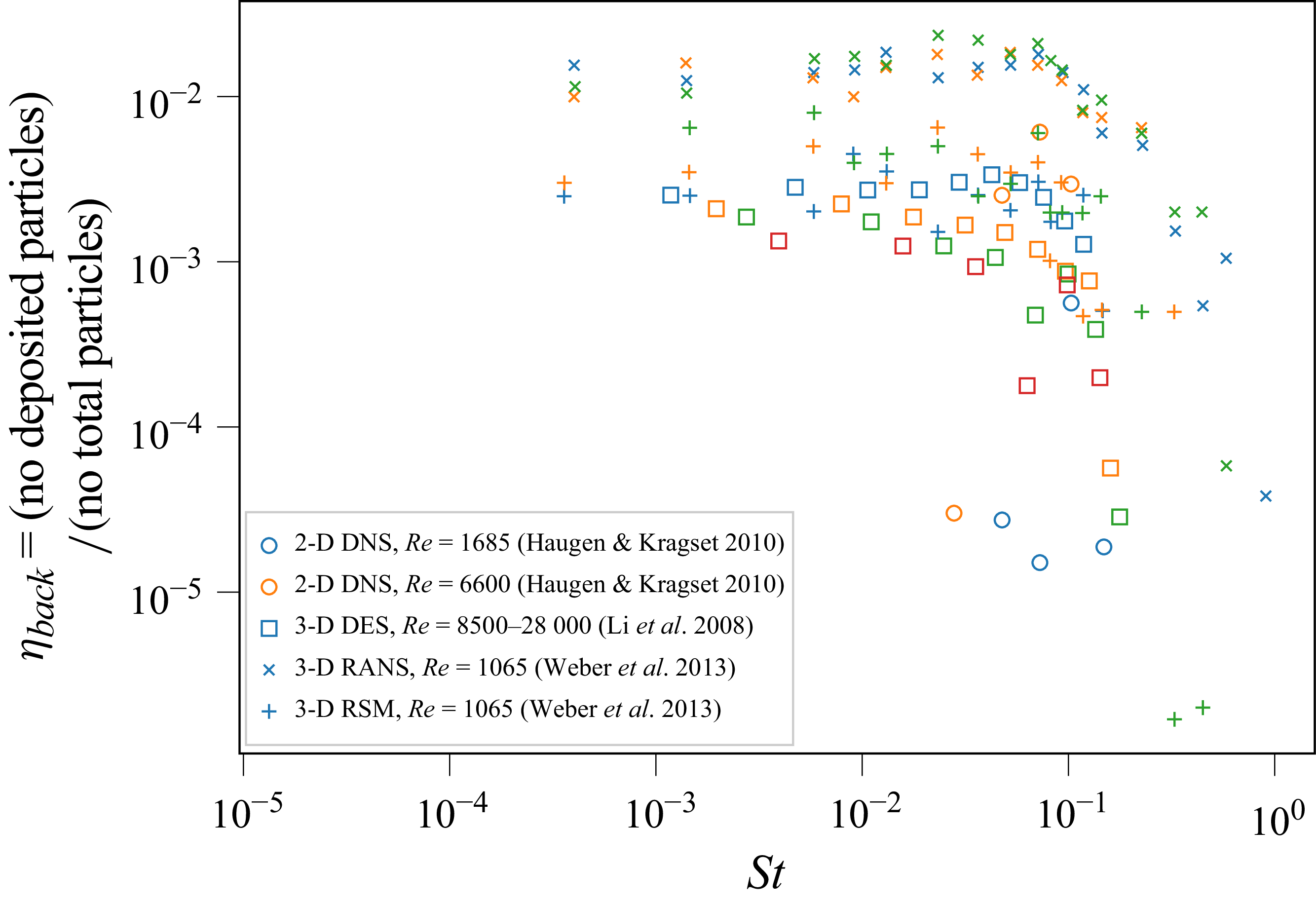


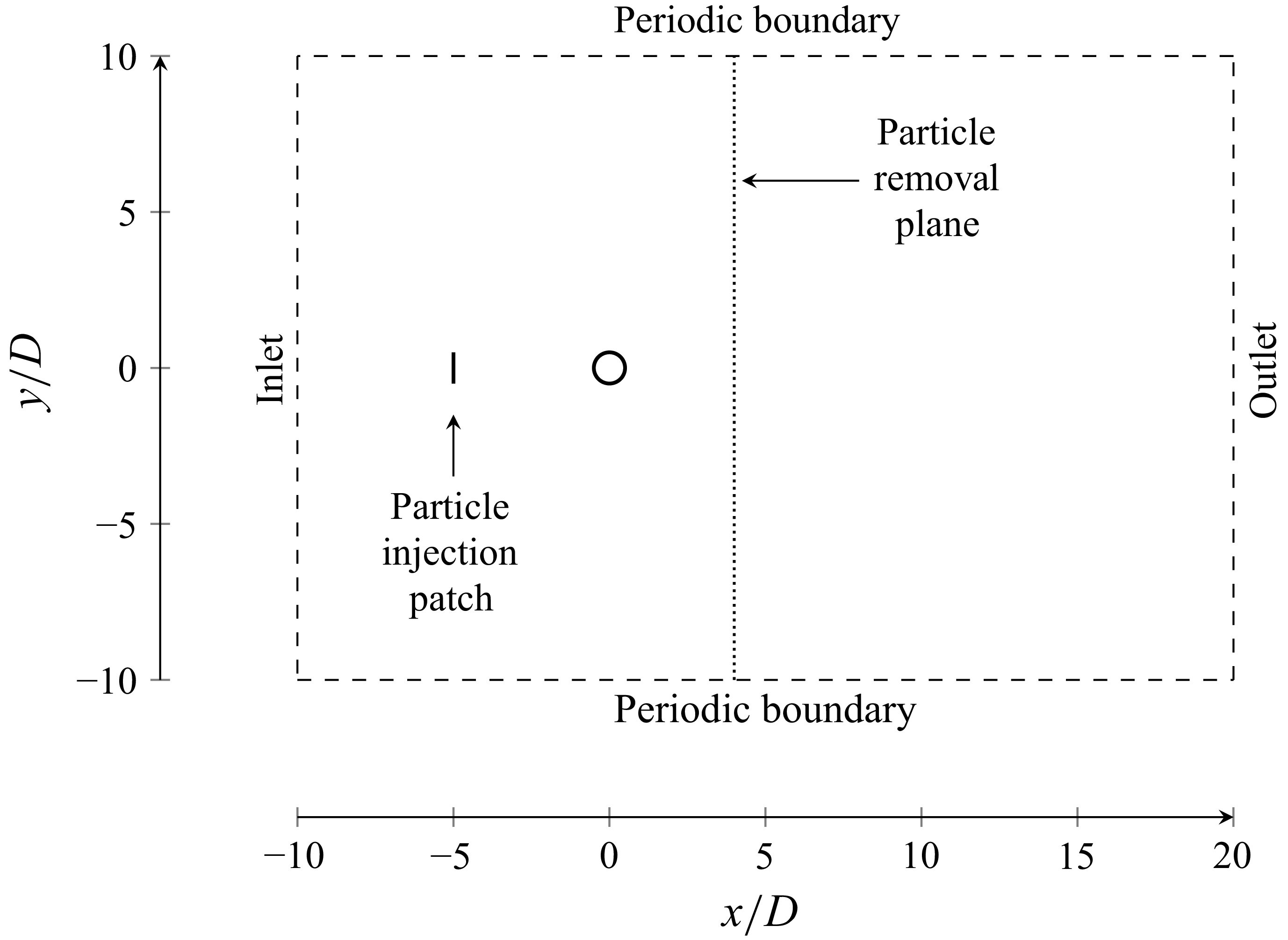


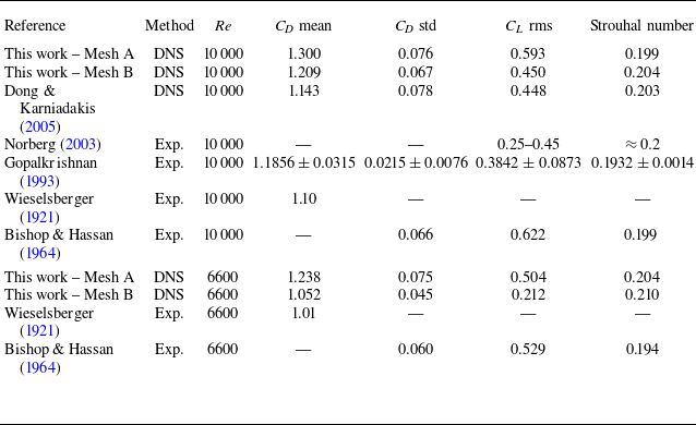


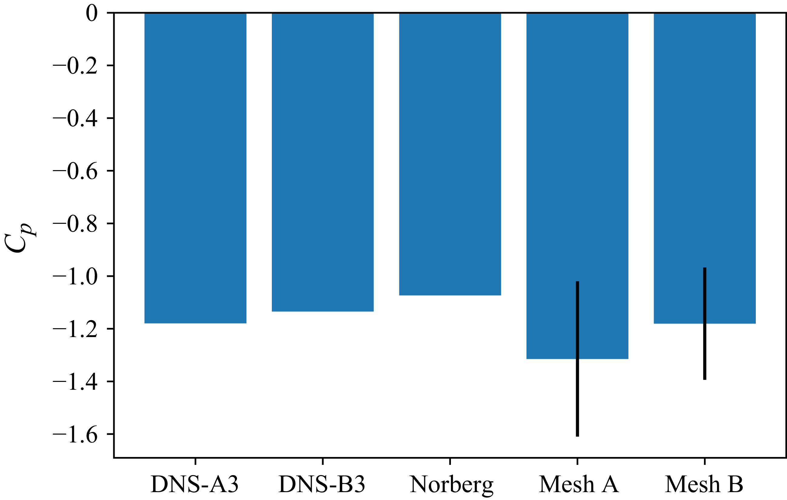


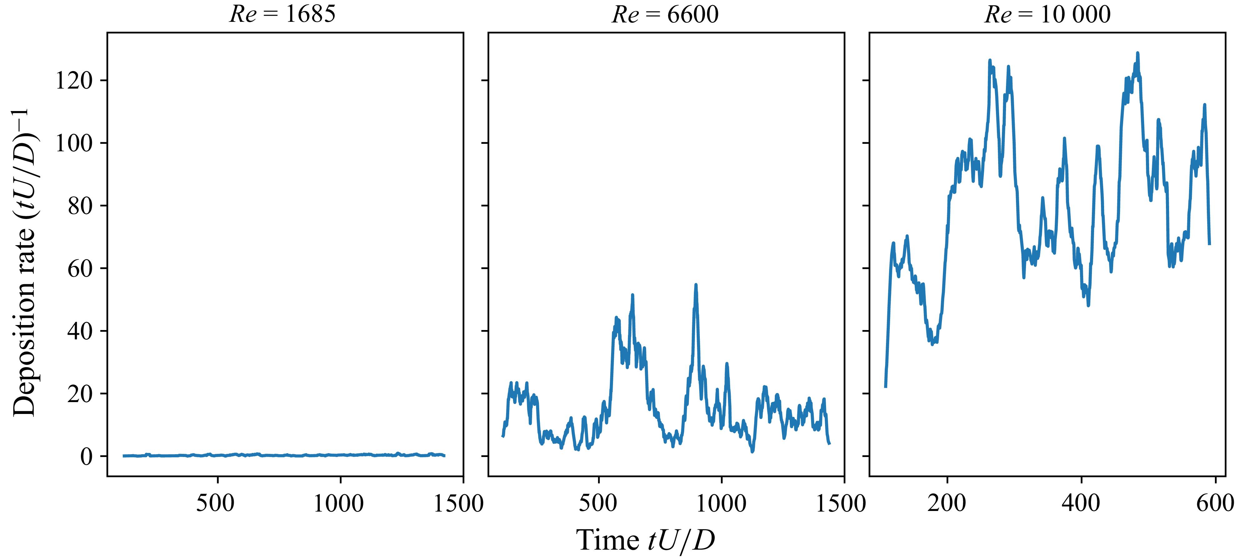

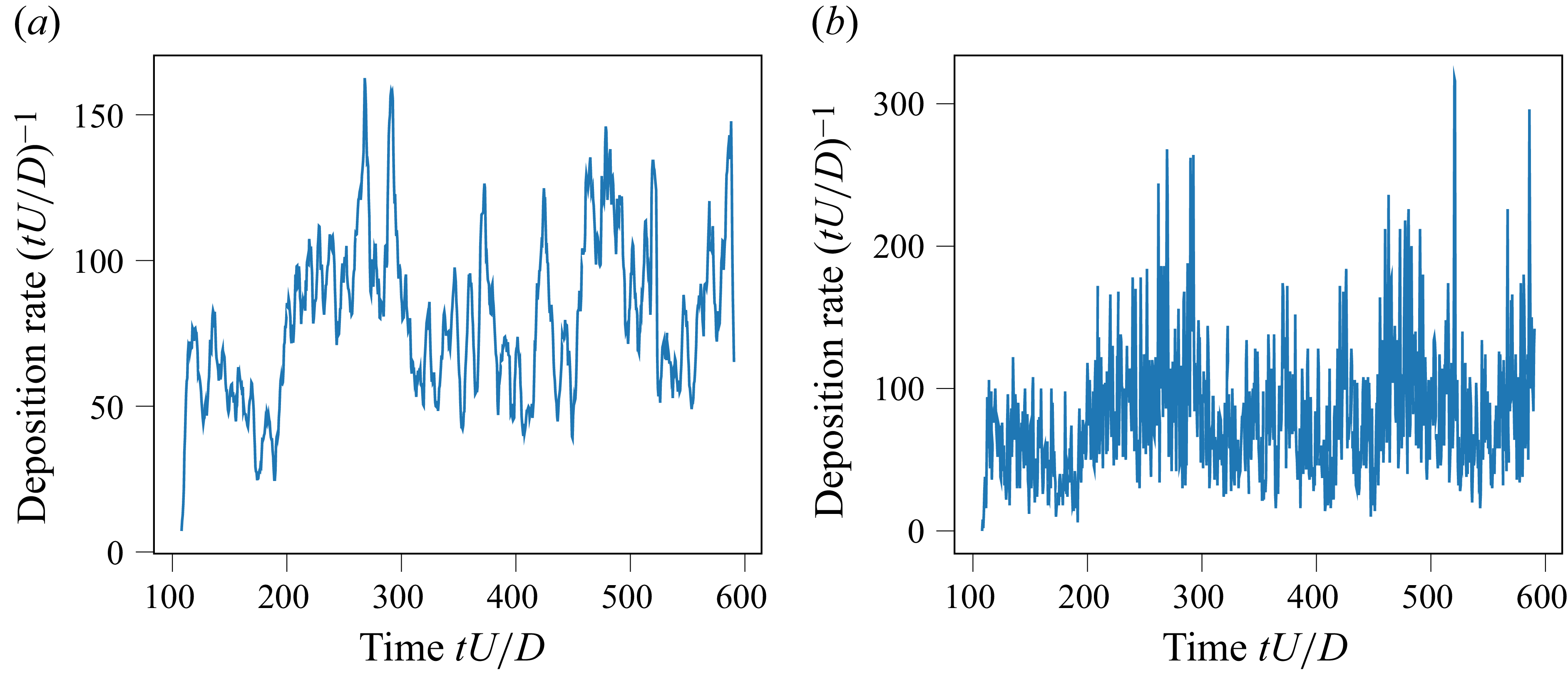


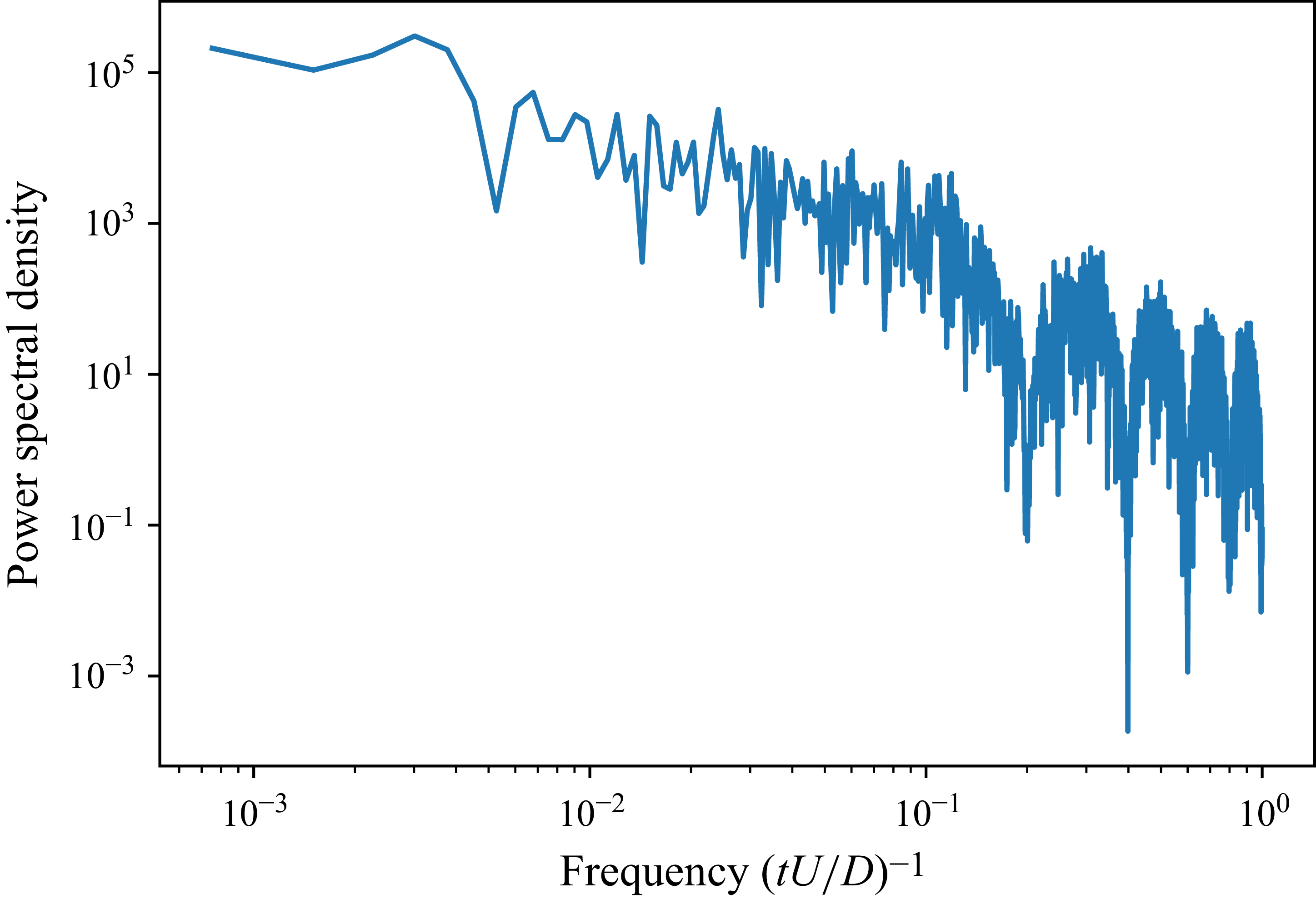


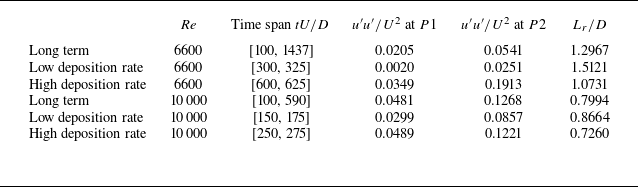


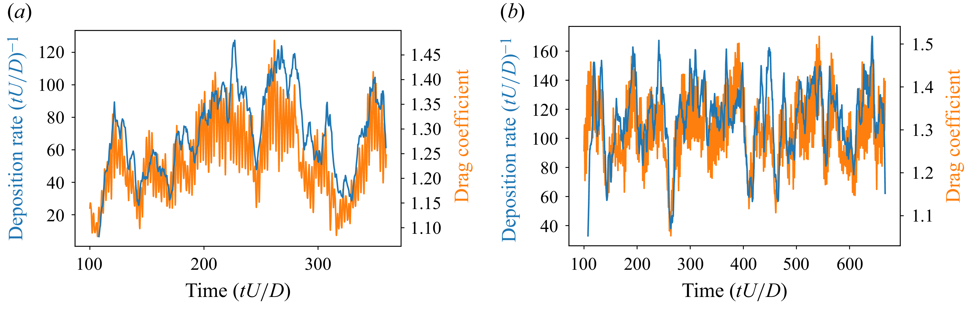


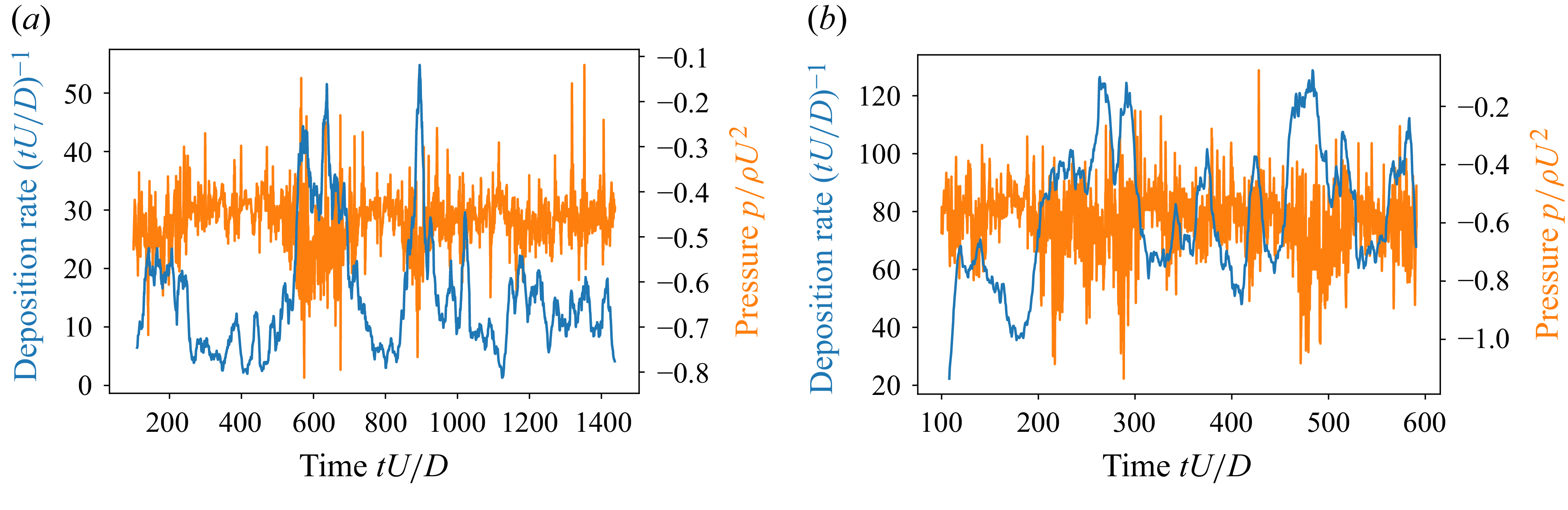


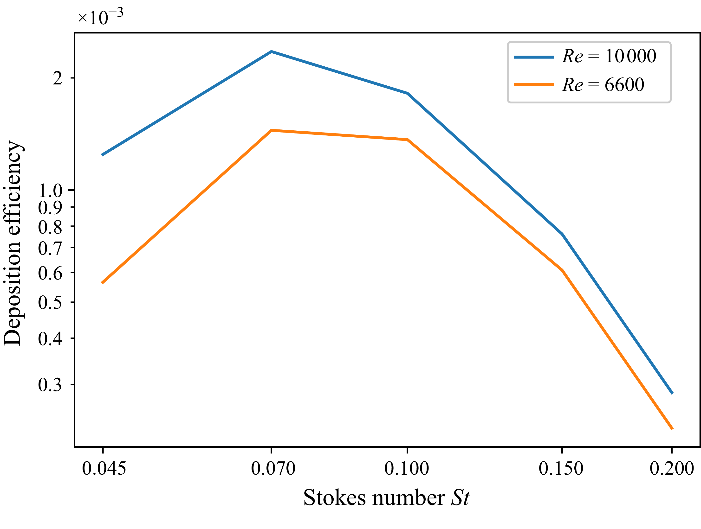


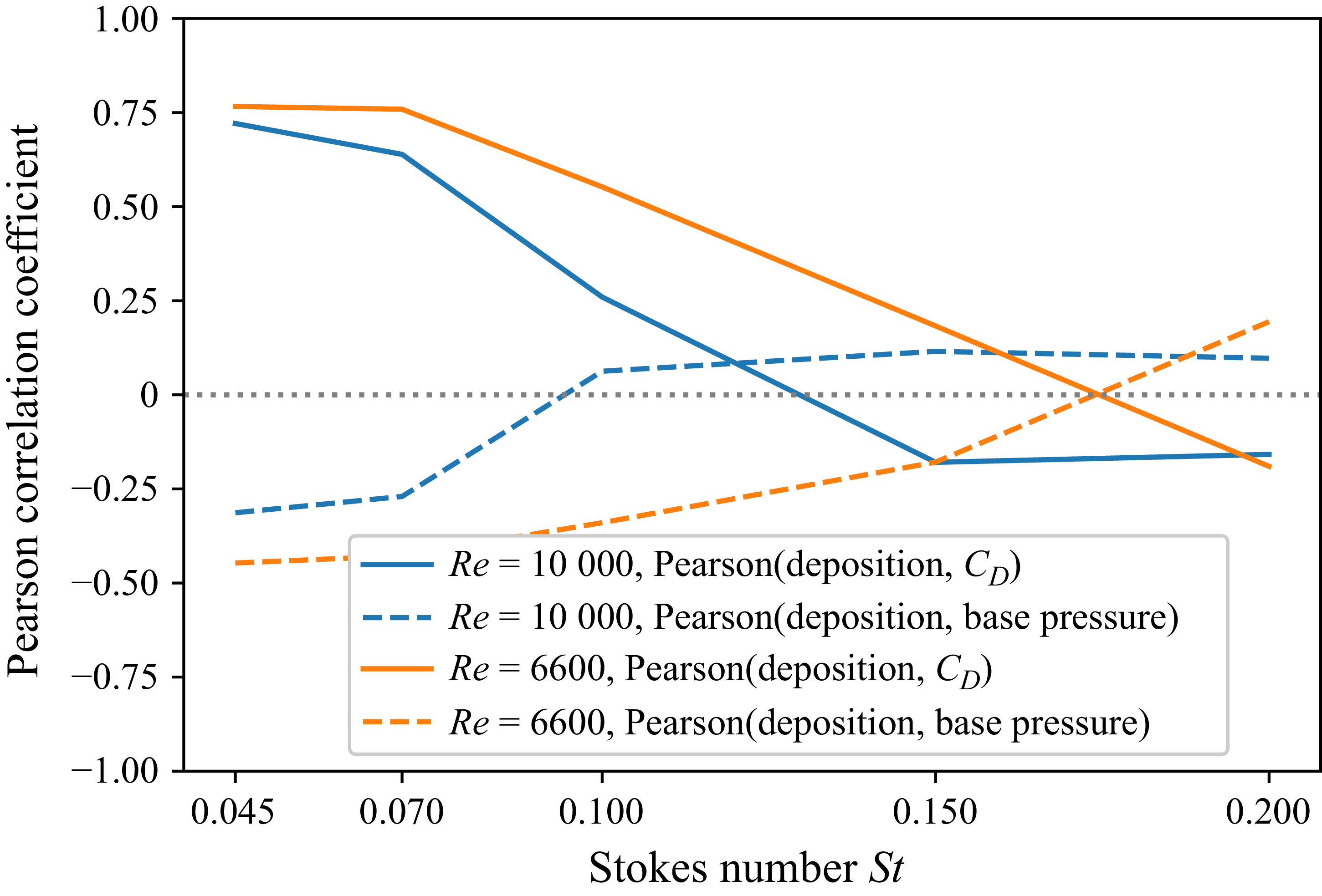


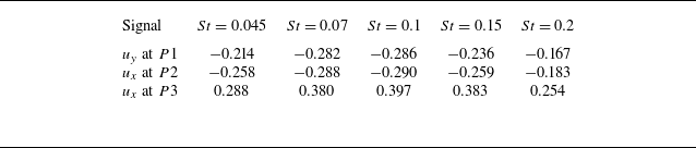


 Open access