


Impact Statement
Progress in climate science and beyond rests more and more on novel data science methods. Of a particular relevance are causal discovery methods that help advance process-based understanding and climate model evaluation. The present work has two main contributions: first, a simplified benchmark model that allows to systematically evaluate causal discovery methods with respect to the typical challenges of gridded climate data, and second, a novel spatiotemporal causal discovery method. The benchmark data will proliferate new methodological developments to gain new insights from widely available climate datasets from satellites or climate model output.
1. Introduction
Global climate is a highly interdependent spatiotemporal dynamical system, with events in one region having profound effects many weeks or months later in other regions thousands of kilometers away. For example, since Sir Gilbert Walker’s seminal works in the 1920s (Walker, Reference Walker1923), the tropical Pacific region has been established as a major driver of global climate. Such remote effects have been termed teleconnections, and their understanding constitutes a key research question both to foster theory building and since knowledge of time-delayed relationships can provide important sources of seasonal predictability (Robertson et al., Reference Robertson, Camargo, Sobel, Vitart and Wang2018). Furthermore, their representation in climate models can guide process-based model evaluation (Eyring et al., Reference Eyring, Cox, Flato, Gleckler, Abramowitz, Caldwell, Collins, Gier, Hall, Hoffman, Hurtt, Jahn, Jones, Klein, Krasting, Kwiatkowski, Lorenz, Maloney, Meehl, Pendergrass, Pincus, Ruane, Russell, Sanderson, Santer, Sherwood, Simpson, Stouffer and Williamson2019; Nowack et al., Reference Nowack, Runge, Eyring and Haigh2020).
Studies to investigate the existence and character of teleconnections have been based on observational data, starting with Bjerknes (Reference Bjerknes1969), but also on numerical modeling, for example, by climate models participating in the Coupled Climate Model Intercomparison Project (Eyring et al., Reference Eyring, Bony, Meehl, Senior, Stevens, Stouffer and Taylor2016). Over the years, a large number of analysis methods have been developed and employed, from standard pairwise correlation, regression, and composite analyses (Von Storch and Zwiers, Reference Von Storch and Zwiers2001) to nonlinear (Balasis et al., Reference Balasis, Donner, Potirakis, Runge, Papadimitriou, Daglis, Eftaxias and Kurths2013) and event-based (Boers et al., Reference Boers, Goswami, Rheinwalt, Bookhagen, Hoskins and Kurths2019), but still pairwise, methods. More recently, linear and nonlinear causal discovery methods (Ebert-Uphoff and Deng, Reference Ebert-Uphoff and Deng2012; Runge et al., Reference Runge, Petoukhov and Kurths2014, Reference Runge, Nowack, Kretschmer, Flaxman and Sejdinovic2019b) have been applied, which attempt to statistically unveil spurious associations due to common drivers or indirect associations. See Runge et al. (Reference Runge, Bathiany, Bollt, Camps-Valls, Coumou, Deyle, Glymour, Kretschmer, Mahecha and Muñoz Marí2019a) for an overview of causal discovery methods.
Since the 1980s, climate observations from satellites have been available as gridded latitude–longitude datasets of many physical climate variables. There are two conceptually different approaches in analyzing teleconnections from such datasets. One is to estimate associations among time series at individual grid locations, leading to the original pointwise teleconnection maps (Wallace and Gutzler, Reference Wallace and Gutzler1981), one-point correlation maps (Von Storch and Zwiers, Reference Von Storch and Zwiers2001), and to the more recent approach of climate network analysis where the associations (typically correlations) among all grid points are treated as a network that can be analyzed with network-theoretic tools (Tsonis and Swanson, Reference Tsonis and Swanson2008; Donges et al., Reference Donges, Zou, Marwan and Kurths2009a,Reference Donges, Zou, Marwan and Kurthsb; Gozolchiani et al., Reference Gozolchiani, Havlin and Yamasaki2011). Associations among grid locations have also been analyzed with causal discovery methods (Deng and Ebert-Uphoff, Reference Deng and Ebert-Uphoff2014).
Another approach is to view the global climate system as driven by a number of major modes of climate variability. Modes such as El Niño–Southern Oscillation (ENSO; Philander, Reference Philander1990), the North Atlantic Oscillation (NAO; Hurrell et al., Reference Hurrell, Kushnir, Ottersen, Hurrell, Kushnir, Ottersen, Visbeck and Visbeck2003), the Pacific Decadal Oscillation (Newman et al., Reference Newman, Alexander, Ault, Cobb, Deser, Di Lorenzo, Mantua, Miller, Minobe and Nakamura2016), the Madden–Julian Oscillation (MJO; Madden and Julian, Reference Madden and Julian1994), or the Stratospheric Polar Vortex (Waugh et al., Reference Waugh, Sobel and Polvani2017) span time scales from weeks to decades and govern global climate from the ocean to stratospheric dynamics. These modes may be viewed as emergent phenomena whereby large regions behave in a coherent way.
To obtain analyzable time series (climate indices), modes need to be extracted from the gridded data. Such a spatial aggregation can be achieved either by expert knowledge to define regional averages or statistical dimension-reduction methods such as principal component analysis (PCA; Von Storch and Zwiers, Reference Von Storch and Zwiers2001), also known as empirical orthogonal functions (EOFs), or its Varimax rotated version (Kaiser, Reference Kaiser1958; Vautard and Ghil, Reference Vautard and Ghil1989). Furthermore, nonlinear dimension-reduction methods exist, for example, through causal effects (Chalupka et al., Reference Chalupka, Eberhardt and Perona2016), kernel methods (Schölkopf and Smola, Reference Schölkopf and Smola2008), or deep learning (Tibau et al., Reference Tibau, Requena-Mesa, Reimers, Denzler, Eyring, Reichstein and Runge2018). Based on these mode estimations, the modes’ teleconnections have been analyzed with a large range of methods from correlation to causal discovery approaches (Ebert-Uphoff and Deng, Reference Ebert-Uphoff and Deng2012; Runge et al., Reference Runge, Petoukhov and Kurths2014, Reference Runge, Petoukhov, Donges, Hlinka, Jajcay, Vejmelka, Hartman, Marwan, Palus and Kurths2015; Kretschmer et al., Reference Kretschmer, Coumou, Donges and Runge2016; Kretschmer et al., Reference Kretschmer, Runge and Coumou2017; Runge et al., Reference Runge, Bathiany, Bollt, Camps-Valls, Coumou, Deyle, Glymour, Kretschmer, Mahecha and Muñoz Marí2019a). There are also works that employ a mixed approach with causal discovery on partly grid point time series and partly modes (Di Capua et al., Reference Di Capua, Runge, Donner, van den Hurk, Turner, Vellore, Krishnan and Coumou2020).
Our focus here is on causal discovery methods both at the grid level and the mode level as a means to gain a more mechanistic process-oriented understanding of teleconnections beyond pairwise correlations. In pairwise correlation, the aim is to test whether pairs of variables are correlated, without accounting for other variables. The challenge of climate data for causal methods is the data’s inherent spatiotemporal nature that has not yet much been addressed in the research community dealing with causal methods (Runge et al., Reference Runge, Bathiany, Bollt, Camps-Valls, Coumou, Deyle, Glymour, Kretschmer, Mahecha and Muñoz Marí2019a). An important drawback of causal methods in climate research is that they cannot be evaluated and benchmarked on real data due to the lack of ground truth, since experimental intervention is not possible in the climate system. The most common approach is to evaluate the physical plausibility of results and their agreement with existing literature. Consequently, it can be challenging to obtain new knowledge not in agreement with the one already established. Benchmark databases and competitions have been a cornerstone of the tremendous success in reaching the extremely fast performance gains in machine learning, for example, of object recognition (Krizhevsky et al., Reference Krizhevsky, Sutskever and Hinton2017). There already exists an online platform hosting challenging time series datasets for causal discovery (http://www.causeme.net; Runge et al., Reference Runge, Bathiany, Bollt, Camps-Valls, Coumou, Deyle, Glymour, Kretschmer, Mahecha and Muñoz Marí2019a), together with an associated competition on pseudoclimate data (Runge et al., Reference Runge, Tibau, Bruhns, Muñoz Marí, Camps-Valls, Escalante and Hadsell2020). Other works, such as the one by Ebert-Uphoff and Deng (Reference Ebert-Uphoff and Deng2017), offer synthetic data to evaluate methods at the grid level. However, for the challenging spatiotemporal nature of the climate system observed as gridded data, no such benchmark exists.
Our paper has two main contributions: first, a novel simplified stochastic climate model, termed spatially aggregated vector-autoregressive (SAVAR) model, that outputs gridded data and provides such a benchmark. Second, we propose a new hybrid causal discovery approach that uses the assumption underlying the SAVAR model and estimates causal relationships at the mode level while yielding causal networks at the grid level. The SAVAR model can be used to benchmark both grid-level causal discovery methods and a combination of dimension-reduction and causal discovery methods. To exemplify the potential of both SAVAR and the novel causal discovery method, we use SAVAR models that emulate the teleconnections of a reanalysis surface pressure dataset to compare the algorithm’s effectiveness against different state-of-the-art algorithms for causal discovery at the grid level.
There are a few related works in the literature. Our model is partially inspired by Linear Inverse Models (Penland and Sardeshmukh, Reference Penland and Sardeshmukh1995). The main difference to our work is twofold. First, the present work explores many of the statistical properties of the model, such as its identifiability and stability. In addition, the model is framed in the domain of climate networks, and the physical implications of potential statistical scenarios are discussed. Second, SAVAR is a versatile model whose purpose is not to directly explain teleconnections or climate relationships, but to improve methods and algorithms that ultimately increase our understanding of the climate system. Another relevant work is the one presented by Fulton and Hegerl (Reference Fulton and Hegerl2021). The authors present a novel method based on Monte Carlo simulations to create ground truth for physically interpretable patterns of modes of climate variability and then evaluate PCA-based dimension reduction against other methods such as slow feature analysis (Wiskott and Sejnowski, Reference Wiskott and Sejnowski2002), optimally persistent patterns (DelSole, Reference DelSole2001), and low-frequency component analysis (Wills et al., Reference Wills, Schneider, Wallace, Battisti and Hartmann2018). In contrast, our work is more focused on modeling and reconstructing the causal relationships among modes. However, their mode generation framework may be integrated to construct more complex SAVAR models.
Our SAVAR model may be seen as a spatiotemporal version of Frankignoul and Hasselmann’s famous stochastic climate model (Hasselmann, Reference Hasselmann1976; Frankignoul and Hasselmann, Reference Frankignoul and Hasselmann1977; Arnold, Reference Arnold2001). Our model also assumes that the fast and chaotic dynamics of weather can be modeled as noise. While Frankignoul and Hasselmann’s model did originally not study the spatial distribution of the fast and chaotic dynamics, here we consider a particular spatiotemporal model where spatial modes of climate variability are viewed as covariant noise representing fast dynamics at the grid level and where teleconnections are modeled as causal relationships between these spatial patterns. In the first place, the goal of this model is not to model particular teleconnections, but their spatiotemporal characteristics and interdependency structure in general for benchmarking purposes.
Using our model as ground truth, we exemplarily compare various methods of causal discovery for common challenges (Runge et al., Reference Runge, Bathiany, Bollt, Camps-Valls, Coumou, Deyle, Glymour, Kretschmer, Mahecha and Muñoz Marí2019a). Our model can flexibly be adapted to help researchers select the best causal method according to the challenges of their data as well as the assumptions they are willing to make. If the assumptions underlying the SAVAR model are fulfilled, we find in our experiments that our grid-level causal method is orders of magnitude better than baseline causal discovery methods, which do not make such assumptions about a mode structure and attempt to directly infer the causal graph at the grid level.
Improved causal discovery methods for spatiotemporal climate data are important to advance process-based understanding. Furthermore, the ability of a climate model to simulate the modes’ causal interdependencies can be used as a key component of model evaluation to guide model improvements and ultimately improved climate projections (Eyring et al., Reference Eyring, Cox, Flato, Gleckler, Abramowitz, Caldwell, Collins, Gier, Hall, Hoffman, Hurtt, Jahn, Jones, Klein, Krasting, Kwiatkowski, Lorenz, Maloney, Meehl, Pendergrass, Pincus, Ruane, Russell, Sanderson, Santer, Sherwood, Simpson, Stouffer and Williamson2019; Falasca et al., Reference Falasca, Bracco, Nenes and Fountalis2019; Hall et al., Reference Hall, Cox, Huntingford and Klein2019; Nowack et al., Reference Nowack, Runge, Eyring and Haigh2020).
The paper has two main parts: first, essential definitions are introduced along with a description of some of the most widespread algorithms and methods. We note that the methods described do not represent an exhaustive list, as there are many more approaches. The second part introduces our own contributions, the SAVAR benchmark model and a new causal discovery algorithm at the grid level. Specifically, in Section 2, we give an overview of teleconnection analysis methods comprising causal discovery methods both in combination with dimension-reduction methods and at the grid level. Here, we also introduce our novel method for causal discovery directly at the grid level. In Section 3, we introduce our proposed benchmark SAVAR model, briefly develop its statistical properties, and give an analysis example. Section 4 uses the SAVAR model to benchmark different teleconnection analysis methods. Finally, Sections 5 and 6 provide a discussion and conclusions.
2. Teleconnection Analysis Approaches
Teleconnection analysis methods may be classified with respect to two different perspectives (Figure 1): first, whether they consider grid-level time series or mode time series extracted through dimension-reduction methods, and second, whether they are based on correlations or causal discovery. These two aspects are developed in the subsequent subsections where we exemplarily review a range of methods spanning these methodological possibilities. We will refer to the estimation of interdependencies among a number of time series variables as network estimation, be it among climate mode index time series or among grid-level time series.
Overview of network estimation methods from two perspectives: nodes can be defined as individual grid locations or at the mode level (vertical dimension). Links can be based on correlation or causation (horizontal dimension). For instance, some nodes in a network may be at the node level and others at the grid level (e.g., correlation maps of El Niño–Southern Oscillation). Causal links may be defined in the bivariate Granger causality case or in a multivariate framework with PCMCI.

2.1. Correlation and causal discovery
The horizontal axis in Figure 1 depicts the correlation–causation dimension with correlation-based approaches on the left and a full multivariate causal discovery framework with multivariate Granger causality, the PCMCI framework (Runge et al., Reference Runge, Nowack, Kretschmer, Flaxman and Sejdinovic2019b), or many other methods (Runge et al., Reference Runge, Bathiany, Bollt, Camps-Valls, Coumou, Deyle, Glymour, Kretschmer, Mahecha and Muñoz Marí2019a) on the right. In between a pure correlation and full multivariate causal discovery framework, there is also a middle ground. Causal links may, for example, be defined in the bivariate Granger causality (Lozano et al., Reference Lozano, Li, Niculescu-Mizil, Liu, Perlich, Hosking and Abe2009; Attanasio et al., Reference Attanasio, Pasini and Triacca2013; Barnett and Seth, Reference Barnett and Seth2015) sense, which only partially accounts for confounders. For real applications, dozens of modes have been identified in the climate literature (De Viron et al., Reference De Viron, Dickey and Ghil2013). Their pairwise statistical relationships can be represented by graphs or networks.
2.1.1. Correlation and bivariate dependency analysis
The most common and simple approach to estimate a teleconnection network from time series (either at the grid level or from climate indices) consists in estimating the (Pearson) correlation among time-lagged variables (up to a maximum time lag $ {\tau}_{\mathrm{max}} $
). Then a network (graph)
$ {\tau}_{\mathrm{max}} $
). Then a network (graph) $ \hat{\mathcal{G}} $
among the time series can be obtained by considering only significant correlations for each time series pair at a particular time lag. That is,
$ \hat{\mathcal{G}} $
among the time series can be obtained by considering only significant correlations for each time series pair at a particular time lag. That is, $ \hat{\mathcal{G}} $
contains an edge from
$ \hat{\mathcal{G}} $
contains an edge from $ {X}_{t-\tau}^i $
to
$ {X}_{t-\tau}^i $
to $ {X}_t^j $
if p-value
$ {X}_t^j $
if p-value $ \left({X}_{t-\tau}^i,{X}_t^j\right)\le \hskip0.35em \alpha $
, where
$ \left({X}_{t-\tau}^i,{X}_t^j\right)\le \hskip0.35em \alpha $
, where $ \alpha $
is the significance level and the p-value can be based on a t-statistic.
$ \alpha $
is the significance level and the p-value can be based on a t-statistic.
Next to the binary adjacency matrix $ \hat{\mathcal{G}} $
, one can encode the strength of lagged links in a matrix
$ \hat{\mathcal{G}} $
, one can encode the strength of lagged links in a matrix $ \Phi \left(\tau \right) $
, where
$ \Phi \left(\tau \right) $
, where $ {\Phi}^{ij}\left(\tau \right) $
denotes the strength of the link between
$ {\Phi}^{ij}\left(\tau \right) $
denotes the strength of the link between $ {X}_{t-\tau}^i $
and
$ {X}_{t-\tau}^i $
and $ {X}_t^j $
as quantified by a correlation coefficient or a standardized regression (
$ {X}_t^j $
as quantified by a correlation coefficient or a standardized regression ( $ {\Phi}^{ij}\left(\tau \right)\hskip0.35em =\hskip0.35em 0 $
if no link exists). Correlation is normalized in
$ {\Phi}^{ij}\left(\tau \right)\hskip0.35em =\hskip0.35em 0 $
if no link exists). Correlation is normalized in $ \left[-1,1\right] $
, and standardized regression coefficients are in units of standard deviations of the respective variables.
$ \left[-1,1\right] $
, and standardized regression coefficients are in units of standard deviations of the respective variables.
While Pearson correlation makes an assumption of linearity of the underlying dependencies, a range of measures exists for the nonlinear case, such as mutual information (Balasis et al., Reference Balasis, Donner, Potirakis, Runge, Papadimitriou, Daglis, Eftaxias and Kurths2013). However, they are only about the form of the statistical dependency and have nothing to do with causality which requires additional assumptions and the ability to account for confounders.
A next step toward causality is to employ bivariate dependency methods such as bivariate Granger causality (Granger, Reference Granger1969; Barnett and Seth, Reference Barnett and Seth2015) or Transfer entropy (Schreiber, Reference Schreiber2000). The latter two at least account for the confounding effect of autocorrelation. However, all these methods share the characteristic that they are bivariate, do not consider the confounding effect of other variables, and cannot deal with contemporaneous causal relationships. Among others, two variables can be statistically dependent because there is a direct relationship between them (i.e., one is the cause of the other) or because they both have a common cause that makes their values co-vary. Additionally, common causes may bias the estimation of the correlation coefficient when this is estimated through bivariate regression. In such cases, it is important to go beyond correlation and move to causal discovery.
2.1.2. Causal discovery
Causal discovery based on the Granger Causality paradigm has been applied to climate research as early as 1997 (Kaufmann and Stern, Reference Kaufmann and Stern1997), but a full formalization of the causal discovery problem beyond Granger causality is more recent (Spirtes et al., Reference Spirtes, Glymour and Scheines2000; see Runge et al., Reference Runge, Bathiany, Bollt, Camps-Valls, Coumou, Deyle, Glymour, Kretschmer, Mahecha and Muñoz Marí2019a, for an overview of causal discovery in the context of Earth sciences).
Causal inference and causal discovery share a common framework, and both focus on uncovering the underlying causal relationships in a system. The difference between the two terms is that causal discovery, sometimes also called causal structural learning, focuses on estimating the graph that represents the qualitatively relationships, that is, whether or not a causal link between two nodes in the graph exists. Causal inference, sometimes also being termed causal effect estimation, on the other hand, aims to determine the quantitative causal effects of the variables among each other.
To formalize the causal discovery task, we briefly introduce the idea of an underlying structural causal model (SCM) and some graph terminology. Consider multivariate time series $ {\mathbf{X}}^j\hskip0.35em =\hskip0.35em \left({X}_t^j,{X}_{t-1}^j,\dots \right) $
for
$ {\mathbf{X}}^j\hskip0.35em =\hskip0.35em \left({X}_t^j,{X}_{t-1}^j,\dots \right) $
for $ j\hskip0.35em =\hskip0.35em 1,\dots, N $
that follow a process model described by
$ j\hskip0.35em =\hskip0.35em 1,\dots, N $
that follow a process model described by
 $$ {X}_t^j\hskip0.35em := \hskip0.35em {f}_j\left(\mathcal{P}\left({X}_t^j\right),{\eta}_t^j\right)\hskip1em \mathrm{with}\hskip0.35em j\hskip0.35em =\hskip0.70em 1,\dots, N. $$
Here, the functions $ {f}_j $
express how the variables
$ {f}_j $
express how the variables $ {X}_t^j $
depend on their drivers, or parents in graph terminology,
$ {X}_t^j $
depend on their drivers, or parents in graph terminology, $ \mathcal{P}\left({X}_t^j\right)\subseteq \left({\mathbf{X}}_t,{\mathbf{X}}_{t-1},\dots, {\mathbf{X}}_{t-p}\right) $
. Here,
$ \mathcal{P}\left({X}_t^j\right)\subseteq \left({\mathbf{X}}_t,{\mathbf{X}}_{t-1},\dots, {\mathbf{X}}_{t-p}\right) $
. Here, $ {\mathbf{X}}_t\hskip0.35em =\hskip0.35em \left({X}_t^1,{X}_t^2,\dots, {X}_t^N\right) $
and
$ {\mathbf{X}}_t\hskip0.35em =\hskip0.35em \left({X}_t^1,{X}_t^2,\dots, {X}_t^N\right) $
and $ p $
is the order of the process. If the noise variables
$ p $
is the order of the process. If the noise variables $ {\eta}_t^j $
are jointly independent and there are no cycles, then the SCM is a Markovian model. When assuming stationarity, the causal relationship of the pair of variables
$ {\eta}_t^j $
are jointly independent and there are no cycles, then the SCM is a Markovian model. When assuming stationarity, the causal relationship of the pair of variables $ \left({X}_{t-\tau}^i,{X}_t^j\right) $
is the same as that of all time-shifted pairs
$ \left({X}_{t-\tau}^i,{X}_t^j\right) $
is the same as that of all time-shifted pairs $ \left({X}_{t^{\prime }-\tau}^i,{X}_{t^{\prime}}^j\right) $
. This is why below we can fix one variable at time
$ \left({X}_{t^{\prime }-\tau}^i,{X}_{t^{\prime}}^j\right) $
. This is why below we can fix one variable at time $ t $
and take
$ t $
and take $ \tau \ge 0 $
. Given such an SCM, the corresponding causal graph (
$ \tau \ge 0 $
. Given such an SCM, the corresponding causal graph ( $ \mathcal{G} $
) is defined as follows: the nodes are given by the
$ \mathcal{G} $
) is defined as follows: the nodes are given by the $ {\mathbf{X}}^j $
at different time points
$ {\mathbf{X}}^j $
at different time points $ t $
and a link
$ t $
and a link $ {X}_{t-\tau}^i\to {X}_t^j $
exists if
$ {X}_{t-\tau}^i\to {X}_t^j $
exists if $ {X}_{t-\tau}^i\in \mathcal{P}\left({X}_t^j\right) $
. This causal link indicates that
$ {X}_{t-\tau}^i\in \mathcal{P}\left({X}_t^j\right) $
. This causal link indicates that $ {X}_{t-\tau}^i $
drives
$ {X}_{t-\tau}^i $
drives $ {X}_t^j $
, and, analogously,
$ {X}_t^j $
, and, analogously, $ {X}_{t-\tau}^i $
is a cause of
$ {X}_{t-\tau}^i $
is a cause of $ {X}_t^j $
, in the sense that
$ {X}_t^j $
, in the sense that $ {X}_{t-\tau}^i $
is in the right-hand side of the equation that defines
$ {X}_{t-\tau}^i $
is in the right-hand side of the equation that defines $ {X}_t^j $
in the SCM. We call links within a variable
$ {X}_t^j $
in the SCM. We call links within a variable $ {\mathbf{X}}^j $
autodependencies and links between different variables cross-dependencies. In the following, we only consider the case where links are time-lagged, that is,
$ {\mathbf{X}}^j $
autodependencies and links between different variables cross-dependencies. In the following, we only consider the case where links are time-lagged, that is, $ \mathcal{P}\left({X}_t^j\right)\subseteq \left({\mathbf{X}}_{t-1},\dots, {\mathbf{X}}_{t-p}\right) $
.
$ \mathcal{P}\left({X}_t^j\right)\subseteq \left({\mathbf{X}}_{t-1},\dots, {\mathbf{X}}_{t-p}\right) $
.
For such an SCM, Figure 1 illustrates the difference between correlation and causation. Consider four processes (e.g., four climate modes) $ {X}^1,{X}^2,{X}^3,{X}^4 $
that are coupled as shown in Figure 1 by some linear or potentially very complex functional dependencies, for example,
$ {X}^1,{X}^2,{X}^3,{X}^4 $
that are coupled as shown in Figure 1 by some linear or potentially very complex functional dependencies, for example,
 $$ {X}_t^1\hskip0.35em =\hskip0.35em {a}_1{X}_{t-1}^1+{\eta}_t^1, $$
 $$ {X}_t^2\hskip0.35em =\hskip0.35em {a}_2{X}_{t-1}^2+{b}_2{X}_{t-2}^1+{\eta}_t^2, $$
 $$ {X}_t^3\hskip0.35em =\hskip0.35em {a}_3{X}_{t-1}^3-{b}_3{X}_{t-2}^1+{\eta}_t^3, $$
 $$ {X}_t^4\hskip0.35em =\hskip0.35em {a}_4{X}_{t-1}^4+{b}_4{X}_{t-2}^3+{\eta}_t^4. $$
The goal of causal discovery (lower right side in Figure 1) is to estimate these direct interdependencies and their time lags. On the other hand, here a pairwise correlation analysis (lower left side in Figure 1) would yield spurious dependencies due to common drivers (e.g., $ {X}^2\leftarrow {X}^1\to {X}^3 $
), transitive indirect paths (e.g.,
$ {X}^2\leftarrow {X}^1\to {X}^3 $
), transitive indirect paths (e.g., $ {X}^1\to {X}^3\to {X}^4 $
), or combinations thereof. Autocorrelation in the modes typically leads to many more connections, also in the reverse direction.
$ {X}^1\to {X}^3\to {X}^4 $
), or combinations thereof. Autocorrelation in the modes typically leads to many more connections, also in the reverse direction.
There are many causal discovery methods for time series (see Runge et al., Reference Runge, Bathiany, Bollt, Camps-Valls, Coumou, Deyle, Glymour, Kretschmer, Mahecha and Muñoz Marí2019a, for an overview). We here consider the PCMCI method (Runge, Reference Runge2018; Runge et al., Reference Runge, Nowack, Kretschmer, Flaxman and Sejdinovic2019b), which has been applied already in a wide range of scenarios (Kretschmer et al., Reference Kretschmer, Coumou, Donges and Runge2016, Reference Kretschmer, Runge and Coumou2017; Di Capua et al., Reference Di Capua, Runge, Donner, van den Hurk, Turner, Vellore, Krishnan and Coumou2020; Krich et al., Reference Krich, Runge, Miralles, Migliavacca, Perez-Priego, El-Madany, Carrara and Mahecha2020; Nowack et al., Reference Nowack, Runge, Eyring and Haigh2020). PCMCI is an adaptation of the conditional independence-based PC algorithm (named after its inventors Peter Spirtes and Clark Glymour; Spirtes et al., Reference Spirtes, Glymour and Scheines2000) that addresses strong autocorrelations in time series via the use of a momentary conditional independence (MCI) test. PCMCI, as part of the conditional independence-based framework, has the advantage that it can flexibly account for various functional causal relations and different data types (continuous and categorical, and univariate and multivariate).
The central idea is to iteratively test whether two variables are statistically independent conditional on any subset of the other variables at any time lag. Two variables $ X $
and
$ X $
and $ Y $
are conditionally independent given a (potentially multivariate) variable
$ Y $
are conditionally independent given a (potentially multivariate) variable $ Z $
, denoted by
$ Z $
, denoted by $ X\perp \hskip-2pt \perp \hskip2pt Y\mid Z $
, if
$ X\perp \hskip-2pt \perp \hskip2pt Y\mid Z $
, if $ p\left(x,y|z\right)\hskip0.35em =\hskip0.35em p\left(x|z\right)p\left(y|z\right)\forall x,y,z $
, where
$ p\left(x,y|z\right)\hskip0.35em =\hskip0.35em p\left(x|z\right)p\left(y|z\right)\forall x,y,z $
, where $ p $
denotes the associated probability density functions. In the example in the lower part of Figure 1 assuming that no autocorrelations are present (
$ p $
denotes the associated probability density functions. In the example in the lower part of Figure 1 assuming that no autocorrelations are present ( $ {a}_i\hskip0.35em =\hskip0.35em 0 $
),
$ {a}_i\hskip0.35em =\hskip0.35em 0 $
), $ {X}^2 $
and
$ {X}^2 $
and $ {X}^3 $
are correlated due to the common driver
$ {X}^3 $
are correlated due to the common driver $ {X}^1 $
, that is,
$ {X}^1 $
, that is, $ {X}_t^2\perp \hskip-2pt \perp \hskip2pt {X}_t^3 $
. However, they become independent once
$ {X}_t^2\perp \hskip-2pt \perp \hskip2pt {X}_t^3 $
. However, they become independent once $ {X}^1 $
is taken into account,
$ {X}^1 $
is taken into account, $ {X}_t^2\perp \hskip-2pt \perp \hskip2pt {X}_t^3\mid {X}_{t-2}^1 $
. To practically test this hypothesis, there exist a large variety of conditional independence tests (see Runge, Reference Runge2018; Runge et al., Reference Runge, Nowack, Kretschmer, Flaxman and Sejdinovic2019b). For linear relationships and Gaussian distributed variables, partial correlation can be used. The partial correlation of two variables
$ {X}_t^2\perp \hskip-2pt \perp \hskip2pt {X}_t^3\mid {X}_{t-2}^1 $
. To practically test this hypothesis, there exist a large variety of conditional independence tests (see Runge, Reference Runge2018; Runge et al., Reference Runge, Nowack, Kretschmer, Flaxman and Sejdinovic2019b). For linear relationships and Gaussian distributed variables, partial correlation can be used. The partial correlation of two variables $ X $
and
$ X $
and $ Y $
given a set of variables
$ Y $
given a set of variables $ Z $
is defined as the correlation between the residuals resulting from fitting linear regressions of each
$ Z $
is defined as the correlation between the residuals resulting from fitting linear regressions of each $ X $
and
$ X $
and $ Y $
on
$ Y $
on $ Z $
. To test the significance of partial correlation, a
$ Z $
. To test the significance of partial correlation, a $ t $
-test can be used. Given
$ t $
-test can be used. Given $ X\perp \hskip-2pt \perp \hskip2pt Y $
and
$ X\perp \hskip-2pt \perp \hskip2pt Y $
and $ X\perp \hskip-2pt \perp \hskip2pt Y\mid Z $
, we say that
$ X\perp \hskip-2pt \perp \hskip2pt Y\mid Z $
, we say that $ Z $
is the set that d-separates
$ Z $
is the set that d-separates $ X $
and
$ X $
and $ Y $
in graph terminology.
$ Y $
in graph terminology.
More formally, given $ N $
time series
$ N $
time series $ {X}_t^j $
for
$ {X}_t^j $
for $ j\hskip0.35em =\hskip0.35em 1,\dots, N $
, PCMCI consists of two stages. First, the PC
$ j\hskip0.35em =\hskip0.35em 1,\dots, N $
, PCMCI consists of two stages. First, the PC $ {}_1 $
condition selection efficiently identifies relevant conditions
$ {}_1 $
condition selection efficiently identifies relevant conditions $ {\hat{\mathrm{\mathcal{B}}}}_t^j $
for all time series variables
$ {\hat{\mathrm{\mathcal{B}}}}_t^j $
for all time series variables $ {X}_t^j $
through a variant of the PC algorithm that removes irrelevant conditions for each of the
$ {X}_t^j $
through a variant of the PC algorithm that removes irrelevant conditions for each of the $ N $
variables by iterative conditional independence testing. Then a link
$ N $
variables by iterative conditional independence testing. Then a link $ {X}_{t-\tau}^i\to {X}_t^j $
is determined by the MCI test:
$ {X}_{t-\tau}^i\to {X}_t^j $
is determined by the MCI test:
 $$ \mathrm{M}\mathrm{C}\mathrm{I}:{X}_{t-\tau}^i\hskip2pt \perp \hskip-2pt \perp \hskip2pt {X}_t^j\hskip2pt \mid \hskip2pt {\hat{\mathrm{B}}}_t^i\hskip2pt \backslash \hskip2pt \{{X}_{t-\tau}^i\},\hskip2pt {\hat{\mathrm{B}}}_{t-\tau}^i. $$
The MCI test conditions on both the parents of $ {X}_t^j $
and the time-shifted parents of
$ {X}_t^j $
and the time-shifted parents of $ {X}_{t-\tau}^i $
. These two stages, PC
$ {X}_{t-\tau}^i $
. These two stages, PC $ {}_1 $
and MCI, serve the following purposes. PC
$ {}_1 $
and MCI, serve the following purposes. PC $ {}_1 $
removes irrelevant lagged conditions (up to some
$ {}_1 $
removes irrelevant lagged conditions (up to some $ {\tau}_{\mathrm{max}} $
) for each variable. A large significance level
$ {\tau}_{\mathrm{max}} $
) for each variable. A large significance level $ {\alpha}_{\mathrm{P}C} $
(e.g.,
$ {\alpha}_{\mathrm{P}C} $
(e.g., $ 0.2 $
) in the tests lets PC
$ 0.2 $
) in the tests lets PC $ {}_1 $
adaptively converge to typically only few relevant conditions that include the causal parents with high probability, but might also include some false positives. The MCI test then addresses false positive control for the highly interdependent time series case. More precisely, while the conditioning on the parents of
$ {}_1 $
adaptively converge to typically only few relevant conditions that include the causal parents with high probability, but might also include some false positives. The MCI test then addresses false positive control for the highly interdependent time series case. More precisely, while the conditioning on the parents of $ {X}_t^j $
(the potential effect) is sufficient to establish conditional independence in the infinite sample limit (Markov property), the additional condition on the lagged parents (parents of
$ {X}_t^j $
(the potential effect) is sufficient to establish conditional independence in the infinite sample limit (Markov property), the additional condition on the lagged parents (parents of $ {X}_{t-\tau}^i $
, the potential cause) leads to a test that is better suited for autocorrelated data. See Runge et al. (Reference Runge, Nowack, Kretschmer, Flaxman and Sejdinovic2019b) for a detailed discussion.
$ {X}_{t-\tau}^i $
, the potential cause) leads to a test that is better suited for autocorrelated data. See Runge et al. (Reference Runge, Nowack, Kretschmer, Flaxman and Sejdinovic2019b) for a detailed discussion.
A causal interpretation of the relationships estimated with PCMCI comes from the standard assumptions in the conditional independence-based framework (Spirtes et al., Reference Spirtes, Glymour and Scheines2000; Runge, Reference Runge2018; Runge et al., Reference Runge, Nowack, Kretschmer, Flaxman and Sejdinovic2019b), namely causal sufficiency, the Causal Markov condition, Faithfulness, non-contemporaneous effects, and stationarity. As demonstrated in Runge et al. (Reference Runge, Nowack, Kretschmer, Flaxman and Sejdinovic2019b), PCMCI has high detection power and controlled false positives also in high-dimensional and strongly autocorrelated time series settings. The main free parameters of PCMCI are the chosen conditional independence test, the maximum time lag $ {\tau}_{\mathrm{max}} $
, and the significance levels
$ {\tau}_{\mathrm{max}} $
, and the significance levels $ \alpha $
in MCI and
$ \alpha $
in MCI and $ {\alpha}_{\mathrm{P}C} $
in PC1, where the latter can be optimized, and the maximum time lag should be larger than the order
$ {\alpha}_{\mathrm{P}C} $
in PC1, where the latter can be optimized, and the maximum time lag should be larger than the order $ p $
of the process (equation (1)).
$ p $
of the process (equation (1)).
Given a significance level $ \alpha $
, the output of PCMCI is the set of parents for all time series variables:
$ \alpha $
, the output of PCMCI is the set of parents for all time series variables:
 $$ {\mathcal{P}}^j\hskip0.35em =\hskip0.35em \left\{{X}_{t-\tau}^i:p-{\mathrm{value}}_{\mathrm{MCI}}\left({X}_{t-\tau}^i,{X}_t^j\right)\le \alpha \hskip1em \forall i\right\}\hskip1em \forall j. $$
The corresponding links then form the estimated graph $ \hat{\mathcal{G}} $
. While PCMCI assumes no contemporaneous links, PCMCI+ (Runge, Reference Runge2022) can be used without this assumption. Furthermore, both algorithms assume causal sufficiency, an assumption that can be relaxed by using LPCMCI (Gerhardus and Runge, Reference Gerhardus and Runge2020).
$ \hat{\mathcal{G}} $
. While PCMCI assumes no contemporaneous links, PCMCI+ (Runge, Reference Runge2022) can be used without this assumption. Furthermore, both algorithms assume causal sufficiency, an assumption that can be relaxed by using LPCMCI (Gerhardus and Runge, Reference Gerhardus and Runge2020).
2.1.3. Causal link quantification
Next to the task of estimating whether a link between two variables exists (detection), a follow-up question is how they are related (quantification; Runge et al., Reference Runge, Nowack, Kretschmer, Flaxman and Sejdinovic2019b). This can take the form of a normalized strength measure such as partial correlation (e.g., MCI partial correlation) or by some statistical model approach. Given the parents estimated from causal discovery, one would then fit a model $ {X}^j\hskip0.35em =\hskip0.35em f\left({\mathcal{P}}^j\right) $
. Under a linear assumption on
$ {X}^j\hskip0.35em =\hskip0.35em f\left({\mathcal{P}}^j\right) $
. Under a linear assumption on $ f $
, this turns into multivariate regression problems for all variables
$ f $
, this turns into multivariate regression problems for all variables $ j $
and results in a coefficient matrix
$ j $
and results in a coefficient matrix $ \Phi $
for every time lag
$ \Phi $
for every time lag $ \tau $
. Then the causal effect between
$ \tau $
. Then the causal effect between $ {X}^i $
and
$ {X}^i $
and $ {X}^j $
at lag
$ {X}^j $
at lag $ \tau $
corresponds to the coefficient
$ \tau $
corresponds to the coefficient $ {\Phi}^{ji}\left(\tau \right) $
. Given a linear SCM
$ {\Phi}^{ji}\left(\tau \right) $
. Given a linear SCM $ {X}_t^2\hskip0.35em =\hskip0.35em {aX}_{t-1}^2+{bX}_{t-2}^1+{\eta}_t^2 $
, then
$ {X}_t^2\hskip0.35em =\hskip0.35em {aX}_{t-1}^2+{bX}_{t-2}^1+{\eta}_t^2 $
, then $ a $
and
$ a $
and $ b $
are
$ b $
are $ {\Phi}^{22}(1) $
and
$ {\Phi}^{22}(1) $
and $ {\Phi}^{21}(2) $
, respectively, if the time series are not standardized. Note that the coefficients not contained in the respective parent sets are defined to be zero, that is,
$ {\Phi}^{21}(2) $
, respectively, if the time series are not standardized. Note that the coefficients not contained in the respective parent sets are defined to be zero, that is, $ {\Phi}^{ji}\left(\tau \right):= 0 $
for
$ {\Phi}^{ji}\left(\tau \right):= 0 $
for $ {X}_{t-\tau}^i\notin {\mathcal{P}}^j $
.
$ {X}_{t-\tau}^i\notin {\mathcal{P}}^j $
.
For the experiments in Section 4, the coefficient matrix $ \Phi $
is estimated with univariate or multivariate linear regression by the method of ordinary least squares (OLS). For the first case, each coefficient is estimated independently. That is, for every
$ \Phi $
is estimated with univariate or multivariate linear regression by the method of ordinary least squares (OLS). For the first case, each coefficient is estimated independently. That is, for every $ {X}_{t-\tau}^i $
in
$ {X}_{t-\tau}^i $
in $ {\mathcal{P}}^j $
, we fit the following linear model:
$ {\mathcal{P}}^j $
, we fit the following linear model:
 $$ {X}_t^j\hskip0.35em =\hskip0.35em {\hat{\Phi}}^{ji}\left(\tau \right){X}_{t-\tau}^i. $$
For the multivariate case for a given variable, the coefficients of its parents are fitted using OLS simultaneously:
 $$ {X}_t^j\hskip0.35em =\hskip0.35em \sum \limits_{X_{t-\tau}^i\in {\mathcal{P}}^j}{\hat{\Phi}}^{ji}\left(\tau \right){X}_{t-\tau}^i. $$
For example, in Figure 1, in order to estimate the coefficients of equation (3) ( $ {\Phi}^{22}(1)\hskip0.35em =\hskip0.35em {a}_2 $
and
$ {\Phi}^{22}(1)\hskip0.35em =\hskip0.35em {a}_2 $
and $ {\Phi}^{21}(2)\hskip0.35em =\hskip0.35em {b}_2 $
), we need to perform a linear regression of
$ {\Phi}^{21}(2)\hskip0.35em =\hskip0.35em {b}_2 $
), we need to perform a linear regression of $ {X}_t^2 $
on its parents (
$ {X}_t^2 $
on its parents ( $ {\mathcal{P}}^2 $
), namely,
$ {\mathcal{P}}^2 $
), namely, $ {X}_{t-1}^2 $
and
$ {X}_{t-1}^2 $
and $ {X}_{t-2}^1 $
. Note that not considering autocorrelation, that is, not controlling for
$ {X}_{t-2}^1 $
. Note that not considering autocorrelation, that is, not controlling for $ {X}_{t-1}^1 $
, would lead to a biased result since
$ {X}_{t-1}^1 $
, would lead to a biased result since $ {X}_{t-1}^1 $
is related to
$ {X}_{t-1}^1 $
is related to $ {X}_t^2 $
through the autocorrelation of
$ {X}_t^2 $
through the autocorrelation of $ {X}^1 $
. Both effects have to be disentangled.
$ {X}^1 $
. Both effects have to be disentangled.
2.2. Grid-level analyses, dimensionality reduction, and climate networks
In the seminal work of Wallace and Gutzler (Reference Wallace and Gutzler1981), correlations among grid location time series were used to investigate so-called teleconnection maps where each grid point’s value was determined by the largest anticorrelation with any other grid point. This led to the discovery of major teleconnection patterns like the NAO. Subsequently, patterns or modes like the NAO, ENSO, and many others became the focus of research, and dimensionality reduction methods were developed to extract typically univariate index time series from gridded satellite datasets. Then teleconnection studies by means of correlation or causal discovery can be carried out among those mode time series. More recently, climate network analysis has emerged as an approach where grid locations are treated as nodes of a network, links are estimated by a variety of methods such as correlation, and the resulting networks are analyzed using complex network methods.
The vertical axis in Figure 1 spans the dimension that defines the variables constituting the nodes in the network from full grid-level to full mode-level analyses. These two aspects will be covered in the following subsections, but we note that methods can also take a middle ground. For instance, some nodes in a network may be at the mode level and others at the grid level (e.g., correlation maps of ENSO; Chronis et al., Reference Chronis, Goodman, Cecil, Buechler, Robertson, Pittman and Blakeslee2008; Di Capua et al., Reference Di Capua, Runge, Donner, van den Hurk, Turner, Vellore, Krishnan and Coumou2020).
2.2.1. Dimension reduction via principal component analysis and Varimax rotation
In the present work, we focus on two common dimensionality reduction methods, PCA and PCA–Varimax, that we also employ in our exemplary benchmark analysis below. In climate research, these are more commonly referred to as EOF analysis and a particular form of rotated empirical orthogonal function analysis. Although we focus on these two methods in the present work, there are also other methods, for example, slow feature analysis (Wiskott and Sejnowski, Reference Wiskott and Sejnowski2002), low-frequency component analysis (Wills et al., Reference Wills, Schneider, Wallace, Battisti and Hartmann2018), or those based on causal feature learning approaches presented by Chalupka et al. (Reference Chalupka, Eberhardt and Perona2016, Reference Chalupka, Eberhardt and Perona2017), as well as further methods based on deep learning (Tibau et al., Reference Tibau, Requena-Mesa, Reimers, Denzler, Eyring, Reichstein and Runge2018, Reference Tibau, Reimers, Requena Mesa and Runge2021; Adsuara et al., Reference Adsuara, Campos-Taberner, García-Haro, Gatta, Romero and Camps-Valls2021).
In PCA, a gridded climate field is partitioned into orthogonal vectors (Von Storch and Zwiers, Reference Von Storch and Zwiers2001). A common way to compute them is through singular value decomposition. Let $ Y\in {\mathrm{\mathbb{R}}}^{L\times T} $
be a climate variable weighted by the square root of the cosine of the latitude with
$ Y\in {\mathrm{\mathbb{R}}}^{L\times T} $
be a climate variable weighted by the square root of the cosine of the latitude with $ L $
grid points, and let
$ L $
grid points, and let $ \Omega $
be its covariance matrix; it is possible to factorize
$ \Omega $
be its covariance matrix; it is possible to factorize $ \Omega $
as
$ \Omega $
as $ \Omega \hskip0.35em =\hskip0.35em {WDW}^{\intercal } $
, where
$ \Omega \hskip0.35em =\hskip0.35em {WDW}^{\intercal } $
, where $ W $
is a matrix whose rows are the eigenvectors of
$ W $
is a matrix whose rows are the eigenvectors of $ \Omega $
and
$ \Omega $
and $ D $
is a diagonal matrix whose entries are the eigenvalues. The derived eigenvalues provide a measure of the variance of each vector. The principal components
$ D $
is a diagonal matrix whose entries are the eigenvalues. The derived eigenvalues provide a measure of the variance of each vector. The principal components $ X $
are the projection of
$ X $
are the projection of $ Y $
onto these eigenvectors,
$ Y $
onto these eigenvectors, $ X\hskip0.35em =\hskip0.35em WY $
. The reduction of the dimension of PCA comes from truncating the matrix
$ X\hskip0.35em =\hskip0.35em WY $
. The reduction of the dimension of PCA comes from truncating the matrix $ W $
by taking only the first
$ W $
by taking only the first $ N $
rows with largest eigenvalues (
$ N $
rows with largest eigenvalues ( $ {W}_N $
) to obtain a lower-dimensional
$ {W}_N $
) to obtain a lower-dimensional $ {X}_N $
. That is,
$ {X}_N $
. That is,
 $$ {X}_N\hskip0.35em =\hskip0.35em {W}_NY. $$
By construction, the PCA patterns and the principal components are each orthogonal. A physical interpretation of PCA vectors is challenging due to the orthogonality constraint since physical systems are not necessarily orthogonal. Furthermore, patterns may be globally spread.
To partially overcome these limitations, PCA patterns can be rotated by some criterion. One such criterion, the Varimax rotation (Kaiser, Reference Kaiser1958; Vautard and Ghil, Reference Vautard and Ghil1989) criterion,
 $$ {R}^{var}\hskip0.35em =\hskip0.35em \underset{R}{\arg \hskip0.1em \max}\left(\frac{1}{L}\sum \limits_n^N\sum \limits_{\mathrm{\ell}}^L{\left({W}_NR\right)}_{n\mathrm{\ell}}^4-\sum \limits_n^N{\left(\frac{1}{L}\sum \limits_{\mathrm{\ell}}^L{\left({W}_NR\right)}_{n\mathrm{\ell}}^2\right)}^2\right), $$
has been used, where $ {R}^{var} $
is a rotation matrix. The objective is to minimize the mode complexity by making the large loadings larger and the small loadings smaller. By using the Varimax rotation matrix
$ {R}^{var} $
is a rotation matrix. The objective is to minimize the mode complexity by making the large loadings larger and the small loadings smaller. By using the Varimax rotation matrix $ {R}^{var} $
,
$ {R}^{var} $
, $ {W}^{var}\hskip0.35em =\hskip0.35em {R}_N^{var}\cdot {W}_N $
is as sparse as possible. Then,
$ {W}^{var}\hskip0.35em =\hskip0.35em {R}_N^{var}\cdot {W}_N $
is as sparse as possible. Then,
 $$ {X}_N^{var}\hskip0.35em =\hskip0.35em {W}_N^{var}Y. $$
This leads to nonorthogonal and often more regionally confined modes. The resulting patterns then may be more physically interpretable. Nevertheless, there is always a degree of arbitrariness, for example, in the number $ N $
of modes retained before rotation or the criterion chosen.
$ N $
of modes retained before rotation or the criterion chosen. $ N $
is then a free parameter of such dimensionality reduction approaches.
$ N $
is then a free parameter of such dimensionality reduction approaches.
Regarding the resulting networks, the nodes of the network are then defined as the modes extracted by such a dimension reduction. The links can then be estimated by correlation or causal discovery approaches. For example, in the mode dimension of Figure 1 (lower part), the variables $ X $
would be defined by multiplying the field
$ X $
would be defined by multiplying the field $ Y $
with
$ Y $
with $ {\hat{W}}_N $
, for
$ {\hat{W}}_N $
, for $ N\hskip0.35em =\hskip0.35em 4 $
, where
$ N\hskip0.35em =\hskip0.35em 4 $
, where $ {\hat{W}}_N $
are the resulting loadings of a dimension-reduction method. Each colored area represents the elements of each of the four rows of
$ {\hat{W}}_N $
are the resulting loadings of a dimension-reduction method. Each colored area represents the elements of each of the four rows of $ {\hat{W}}_N $
. To simplify the notation and since in this work we always truncate
$ {\hat{W}}_N $
. To simplify the notation and since in this work we always truncate $ \hat{W} $
to the true value
$ \hat{W} $
to the true value $ N $
, in the following, we will refer to the estimated weights from dimension-reduction methods (
$ N $
, in the following, we will refer to the estimated weights from dimension-reduction methods ( $ {\hat{W}}_N $
) as
$ {\hat{W}}_N $
) as $ \hat{W} $
.
$ \hat{W} $
.
2.2.2. Climate networks
In the past years, climate network analysis (Tsonis and Swanson, Reference Tsonis and Swanson2008; Donges et al., Reference Donges, Zou, Marwan and Kurths2009a,Reference Donges, Zou, Marwan and Kurthsb; Gozolchiani et al., Reference Gozolchiani, Havlin and Yamasaki2011; Fan et al., Reference Fan, Meng, Ashkenazy, Havlin and Schellnhuber2017; Falasca et al., Reference Falasca, Bracco, Nenes and Fountalis2019) has emerged as another approach to analyze teleconnections. The nodes of a climate network are the individual grid locations of a gridded climate field. Among these, some measure of association (or similarity) is computed, most commonly the Pearson correlation. Then the climate network’s links are defined by thresholding the correlation values. These networks can then be subjected to global and local network-theoretic measures such as the node degree or betweenness centrality as a measure that counts how many shortest paths in a network pass through a given grid point. While this procedure results in a binary undirected network, time-lagged correlations have been employed to define directed networks and many further variants exist (see Donges et al., Reference Donges, Zou, Marwan and Kurths2009b, for an overview). The underlying idea is that emergent properties of a system can be extracted in this way. For example, climate networks have been used to predict ENSO events (Ludescher et al., Reference Ludescher, Gozolchiani, Bogachev, Bunde, Havlin and Schellnhube2014) or to evaluate climate models (Falasca et al., Reference Falasca, Bracco, Nenes and Fountalis2019). Another pairwise network approach, but with event synchronization instead of correlation, was used in Boers et al. (Reference Boers, Goswami, Rheinwalt, Bookhagen, Hoskins and Kurths2019).
Climate network analysis at the grid level has also been approached with causal discovery methods. Notable examples are Ebert-Uphoff and Deng (Reference Ebert-Uphoff and Deng2012) and Deng and Ebert-Uphoff (Reference Deng and Ebert-Uphoff2014), where the authors employ the conditional independence-based PC algorithm to estimate directed networks at the grid level. The causal climate networks were then used to evaluate remote teleconnections and information flows in observational data, as well as changes of the network connectivity due to the forcing of enhanced greenhouse gasses in model data. Here, the links $ {\mathcal{G}}^{ij} $
are between the grid points,
$ {\mathcal{G}}^{ij} $
are between the grid points, $ i,\hskip0.35em j\hskip0.35em =\hskip0.35em 1,\dots, L $
. Other relevant studies define climate networks from the spherical harmonics coefficients obtained from a spectral decomposition of atmospheric data (Zerenner et al., Reference Zerenner, Friederichs, Lehnertz and Hense2014; Samarasinghe et al., Reference Samarasinghe, Deng and Ebert-Uphoff2020).
$ i,\hskip0.35em j\hskip0.35em =\hskip0.35em 1,\dots, L $
. Other relevant studies define climate networks from the spherical harmonics coefficients obtained from a spectral decomposition of atmospheric data (Zerenner et al., Reference Zerenner, Friederichs, Lehnertz and Hense2014; Samarasinghe et al., Reference Samarasinghe, Deng and Ebert-Uphoff2020).
However, there are a number of statistical and interpretational challenges with the causal approach at the grid level. In Sections 4.1.4 and 4.2, we provide an example, and Figure 5 illustrates these challenges. On a statistical side, conducting a causal discovery approach with conditional independence tests among thousands of grid location time series given sample sizes of similar order is much more challenging than among a few climate mode time series. This problem results in low statistical power in detecting individual links (Runge et al., Reference Runge, Nowack, Kretschmer, Flaxman and Sejdinovic2019b). Furthermore, neighboring grid locations often have highly redundant time series (depending also on the grid resolution). Consider the estimation of a causal link between two remote locations. The PC algorithm tests whether these two are conditionally independent given any other subset of grid location time series, including the neighboring ones. Since conditioning on highly redundant time series decreases the dependence between the two remote grid locations, this aggravates the problem of low detection power. In Runge (Reference Runge2018), the redundancy problem is discussed for the extreme case that one variable is a deterministic function of another variable. Moreover, causal discovery methods face computational problems for datasets with hundreds or thousands of variables.
Representation of the Mapped-PCMCI algorithm. (a) Perform a dimensionality reduction method on a gridded dataset to obtain a mapping between the gridded data and its lower-dimensional representation. (b) Apply a causal discovery method to obtain the parents and the estimated causal network from the resulting time series. (c) Estimate the lagged causal effects for all links to obtain a coefficient matrix. (d) “Invert” the dimensionality reduction mapping to obtain the causal network and the causal effects at the grid level.

Illustration of the spatially aggregated vector-autoregressive model. Climate fields $ {\mathbf{y}}_t $
evolving as given in equation (16) are represented by time series on a regular grid. Climate modes of variability are defined by regions
$ {\mathbf{y}}_t $
evolving as given in equation (16) are represented by time series on a regular grid. Climate modes of variability are defined by regions $ {W}_i $
of covariant Gaussian noise
$ {W}_i $
of covariant Gaussian noise $ {\varepsilon}_t\sim \mathcal{N}\left({\mu}_y,{\Sigma}_y\right) $
where
$ {\varepsilon}_t\sim \mathcal{N}\left({\mu}_y,{\Sigma}_y\right) $
where $ {\Sigma}_y $
denotes the spatial covariance matrix of the grid level noise. Time series at the grid level are mapped to the mode level by
$ {\Sigma}_y $
denotes the spatial covariance matrix of the grid level noise. Time series at the grid level are mapped to the mode level by $ {\mathbf{x}}_t=W{\mathbf{y}}_t $
. The interdependencies between the modes (causal network), here represented by black arrows, are defined by
$ {\mathbf{x}}_t=W{\mathbf{y}}_t $
. The interdependencies between the modes (causal network), here represented by black arrows, are defined by $ \Phi $
, where
$ \Phi $
, where $ {\Phi}_{ij}\left(\tau \right) $
denotes the effect of the
$ {\Phi}_{ij}\left(\tau \right) $
denotes the effect of the $ j $
th mode into the
$ j $
th mode into the $ i $
th mode at time lag
$ i $
th mode at time lag $ \tau $
.
$ \tau $
.

Example of a four-mode spatially aggregated vector-autoregressive model and network estimation based on PCA–PCMCI and Varimax–PCMCI. When the algorithm used to detect spatial patterns is not suitable to recover them from data (in this specific case, principal component analysis [PCA]), then both spatial and causal inferred conclusions may be wrong. (a) The ground truth. Each row represents the weight vector of a mode (columns of $ W $
). In red, the underlying causal network is shown (
$ W $
). In red, the underlying causal network is shown ( $ \mathcal{G} $
). (b) The first four components of Varimax estimated weights (
$ \mathcal{G} $
). (b) The first four components of Varimax estimated weights ( $ \hat{W} $
) and in red the estimated PCMCI causal network (
$ \hat{W} $
) and in red the estimated PCMCI causal network ( $ \hat{\mathcal{G}} $
). (c) The first four components of PCA estimated weights (
$ \hat{\mathcal{G}} $
). (c) The first four components of PCA estimated weights ( $ \hat{W} $
) and in red the estimated PCMCI causal network (
$ \hat{W} $
) and in red the estimated PCMCI causal network ( $ \hat{\mathcal{G}} $
).
$ \hat{\mathcal{G}} $
).

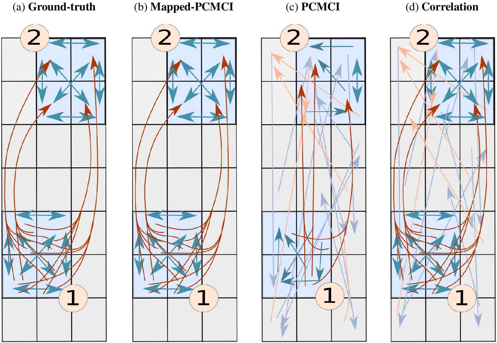
Example of a two-mode spatially aggregated vector-autoregressive model and grid-level network estimations. Ground truth (a), network estimated by Mapped-PCMCI (b), by PCMCI at the grid level (c), and by correlation at the grid level (d). The blue arrows indicate dependencies at lag 1, and the brown arrows indicate dependencies at lag 2. The light blue and light brown arrows indicate a false positive link detected by the method. For the sake of visualization, autodependencies in the same grid point are not shown, and only a small fraction of false positives are shown ( $ \le \hskip0.35em 50\% $
and
$ \le \hskip0.35em 50\% $
and $ \le \hskip0.35em 10\% $
in (c) and (d), respectively). Table 1 shows the performance metrics for each method. Details of the structural causal model can be found in Section 3.4.2.
$ \le \hskip0.35em 10\% $
in (c) and (d), respectively). Table 1 shows the performance metrics for each method. Details of the structural causal model can be found in Section 3.4.2.
Although there is a larger complexity of causal networks at the grid level, there are several reasons for this type of analysis. First, such large networks open the door to introduce concepts and tools from complex network theory (Newman, Reference Newman2018), for example, node centrality measures. In addition, because networks are represented at the grid level, it is possible to trace the effect of a perturbation produced in one grid point to the whole grid through the estimated network. And finally, one can deal with nonstationary networks both in time and space, simultaneously. For example, there can be a change in the shape and the position of a mode distinct from a change in the underlying graph (see Section 5).
2.3. Mapped-PCMCI for causal discovery at the grid level
We present a new method that aims to overcome some of these challenges. The method is based on the assumption that the causal dependencies within a gridded dataset have a lower-dimensional mode representation, in line with the perspective of a number of modes of variability driving global climate variability. The approach consists of four steps:
-
1. Perform a dimensionality reduction method on the gridded data to extract a limited number of N mode time series variables $ \hat{\mathbf{X}}\hskip0.35em =\hskip0.35em \left({\hat{X}}^1,\dots, {\hat{X}}^N\right) $
with corresponding weights (or loadings)
$ \hskip2em \hat{W}\hskip0.35em =\hskip0.35em \left({\hat{W}}^1,\dots, {\hat{W}}^N\right) $
.
$ \hat{\mathbf{X}}\hskip0.35em =\hskip0.35em \left({\hat{X}}^1,\dots, {\hat{X}}^N\right) $
with corresponding weights (or loadings)
$ \hskip2em \hat{W}\hskip0.35em =\hskip0.35em \left({\hat{W}}^1,\dots, {\hat{W}}^N\right) $
. -
2. Apply a causal discovery method to
$ \hat{\mathbf{X}} $
to obtain the parents
$ \left(\mathcal{P}\left({\hat{X}}^1\right),\dots, \mathcal{P}\left({\hat{X}}^N\right)\right) $
and the estimated causal network
$ \hat{\mathcal{G}} $
of the modes. -
3. Estimate (lagged) causal effects for all links to obtain a coefficient matrix
$ \hat{\Phi}\left(\tau \right)\in {\mathrm{\mathbb{R}}}^{N\times N} $
. -
4. “Invert” the dimension reduction, that is, use the modes’ weights
$ \hat{W} $
to map
$ \hat{\Phi}\left(\tau \right) $
back to causal effects among the grid locations. This is done by right- and left-multiplying
$ \hat{\Phi}\left(\tau \right) $
with
$ W $
and its pseudoinverse (
$ {W}^{+} $
), respectively, that is,
$ {\hat{\Phi}}_Y\left(\tau \right)\hskip0.35em =\hskip0.35em {\hat{W}}^{+}\hat{\Phi}\left(\tau \right)\hat{W} $
.


Figure 2 shows a representation of Mapped-PCMCI.
In the first step, we estimate a weight matrix $ \hat{W} $
that projects the original data into a mode space of smaller dimension
$ \hat{W} $
that projects the original data into a mode space of smaller dimension $ N $
, where
$ N $
, where $ N $
is a free parameter. In the next step, we estimate the network
$ N $
is a free parameter. In the next step, we estimate the network $ \hat{\mathcal{G}} $
between these modes by finding the parents of each mode. In the third step, we estimate the causal effect of the links of
$ \hat{\mathcal{G}} $
between these modes by finding the parents of each mode. In the third step, we estimate the causal effect of the links of $ \hat{\mathcal{G}} $
, by fitting a coefficient matrix of the VAR process in the mode space
$ \hat{\mathcal{G}} $
, by fitting a coefficient matrix of the VAR process in the mode space $ \hat{\Phi}\left(\tau \right) $
. Finally, in the last step, we map the information contained in
$ \hat{\Phi}\left(\tau \right) $
. Finally, in the last step, we map the information contained in $ \hat{\mathcal{G}} $
and
$ \hat{\mathcal{G}} $
and $ \hat{\Phi}\left(\tau \right) $
onto the grid space by using
$ \hat{\Phi}\left(\tau \right) $
onto the grid space by using $ \hat{W} $
and its pseudoinverse. Because there are fewer modes than grid points,
$ \hat{W} $
and its pseudoinverse. Because there are fewer modes than grid points, $ \hat{W} $
is not square but need to have a nonzero kernel and using its pseudoinverse implies necessarily some loss of information. However, depending on the underlying assumptions, it may not affect the estimation of
$ \hat{W} $
is not square but need to have a nonzero kernel and using its pseudoinverse implies necessarily some loss of information. However, depending on the underlying assumptions, it may not affect the estimation of $ \Phi \left(\tau \right) $
. For more details, see Section 3 and Appendix B in the Supplementary Material. The third step aims to obtain a spatial grid-level representation of the causal network that has been obtained at the mode level. This is referred to in the literature as a climate network (Donges et al., Reference Donges, Zou, Marwan and Kurths2009a,Reference Donges, Zou, Marwan and Kurthsb), and we offer here a way to obtain a causal climate network. Furthermore, such a representation can be helpful in modeling spatially changing phenomena. A case in point is when we have a climate pattern that regularly changes position and shape, such as the MJO.
$ \Phi \left(\tau \right) $
. For more details, see Section 3 and Appendix B in the Supplementary Material. The third step aims to obtain a spatial grid-level representation of the causal network that has been obtained at the mode level. This is referred to in the literature as a climate network (Donges et al., Reference Donges, Zou, Marwan and Kurths2009a,Reference Donges, Zou, Marwan and Kurthsb), and we offer here a way to obtain a causal climate network. Furthermore, such a representation can be helpful in modeling spatially changing phenomena. A case in point is when we have a climate pattern that regularly changes position and shape, such as the MJO.
The first three steps, dimensionality reduction, causal discovery, and causal effect estimation, can be performed with different methods. In our exemplary benchmark analysis, we employ PCA/Varimax, correlation/PCMCI, and univariate/multivariate regression, respectively. When using PCMCI as the causal discovery method, we refer to this approach as Mapped-PCMCI. In Algorithm 1 in Section C of the Supplementary Material, we provide pseudocode for Mapped-PCMCI with Varimax dimension reduction and a linearity assumption.
Note that in the case of PCA or Varimax, the weight vectors are nonzero everywhere. This would imply that when mapping the causal effects $ \Phi \left(\tau \right) $
from the mode to the grid space, many grid points will be connected to each other. To address this problem, one can either use a significance test to identify for which grid locations the weight vectors are nonsignificant or use a threshold to set small weights to zero. We use here the significance test approach. We have developed a modification of the Varimax algorithm, which we term Varimax
$ \Phi \left(\tau \right) $
from the mode to the grid space, many grid points will be connected to each other. To address this problem, one can either use a significance test to identify for which grid locations the weight vectors are nonsignificant or use a threshold to set small weights to zero. We use here the significance test approach. We have developed a modification of the Varimax algorithm, which we term Varimax $ {}^{+} $
, that uses bootstrap and hypothesis testing to estimate which values of the loadings do not significantly differ from
$ {}^{+} $
, that uses bootstrap and hypothesis testing to estimate which values of the loadings do not significantly differ from $ 0 $
. A detailed description can be found in Appendix C.3 in the Supplementary Material.
$ 0 $
. A detailed description can be found in Appendix C.3 in the Supplementary Material.
3. Benchmarking Teleconnection Analysis Methods—The SAVAR Model
Many of the tremendous performance gains in machine learning, for example, of object recognition (Schmidhuber, Reference Schmidhuber2015) were spurred by open benchmark databases and competitions that allowed for a consistent comparison of methods. In this spirit, the http://www.causeme.net (Runge et al., Reference Runge, Bathiany, Bollt, Camps-Valls, Coumou, Deyle, Glymour, Kretschmer, Mahecha and Muñoz Marí2019a) benchmark platform aims at improving the development of causal discovery methods by hosting multivariate time series datasets with known underlying causal relations. However, for the challenging spatiotemporal nature of the climate system, no such benchmark exists. In the following, we derive a novel model formulation inspired by Frankignoul and Hasselmann’s stochastic climate model that can serve as a benchmark for evaluating dimension-reduction and causal discovery methods.
3.1. Derivation
In Frankignoul and Hasselmann’s model (Hasselmann, Reference Hasselmann1976; Frankignoul and Hasselmann, Reference Frankignoul and Hasselmann1977), the variability of climate is attributed to internal random forcing by the short time scale weather components of the system. For example, the heat balance equation from Frankignoul and Hasselmann (Reference Frankignoul and Hasselmann1977) governing the evolution of an SST anomaly $ T(t) $
at a grid location or regional average is defined as
$ T(t) $
at a grid location or regional average is defined as
 $$ \frac{d}{dt}T(t)\hskip0.35em =\hskip0.35em f\left(T,W\right), $$
where $ f $
is a forcing function determined by various heat fluxes, radiation, and momentum across the air–sea interface. The basic assumption of Frankignoul and Hasselmann’s model is that the characteristic correlation time scale of the atmospheric variables (here, e.g., wind speed)
$ f $
is a forcing function determined by various heat fluxes, radiation, and momentum across the air–sea interface. The basic assumption of Frankignoul and Hasselmann’s model is that the characteristic correlation time scale of the atmospheric variables (here, e.g., wind speed) $ W(t) $
is small compared with the time scale of the response
$ W(t) $
is small compared with the time scale of the response $ T(t) $
. Under an additional linear approximation, the fluctuations
$ T(t) $
. Under an additional linear approximation, the fluctuations $ {T}^{\prime },{W}^{\prime } $
around some mean state can be written as an Ornstein–Uhlenbeck process
$ {T}^{\prime },{W}^{\prime } $
around some mean state can be written as an Ornstein–Uhlenbeck process
 $$ \frac{d}{dt}{T}^{\prime }(t)\hskip0.35em =\hskip0.35em -{\theta}_o{T}^{\prime }(t)+{\sigma}_o{W}^{\prime }(t), $$
for some linear coefficient $ {\theta}_o $
governing a negative slow-acting feedback and
$ {\theta}_o $
governing a negative slow-acting feedback and $ {\sigma}_o $
governing the variance of weather dynamics modeled as the white noise term
$ {\sigma}_o $
governing the variance of weather dynamics modeled as the white noise term $ {W}^{\prime }(t) $
. Converted to a discrete-time representation, the Ornstein–Uhlenbeck process becomes an autoregressive (AR) model
$ {W}^{\prime }(t) $
. Converted to a discrete-time representation, the Ornstein–Uhlenbeck process becomes an autoregressive (AR) model
 $$ {T}_t^{\prime}\hskip0.35em =\hskip0.35em {\tilde{\theta}}_o{T}_{t-1}^{\prime }+{\tilde{\sigma}}_o{W}_t^{\prime }, $$
with the substitutions $ {\tilde{\theta}}_o\hskip0.35em =\hskip0.35em 1-{\theta}_o\Delta t $
and
$ {\tilde{\theta}}_o\hskip0.35em =\hskip0.35em 1-{\theta}_o\Delta t $
and $ {\tilde{\sigma}}_o\hskip0.35em =\hskip0.35em {\sigma}_o\sqrt{\Delta t} $
.
$ {\tilde{\sigma}}_o\hskip0.35em =\hskip0.35em {\sigma}_o\sqrt{\Delta t} $
.
Our goal is to extend this idea to model spatially resolved modes of climate variability and their time-delayed teleconnections, resulting in a gridded data output that can serve to benchmark both dimension-reduction and network estimation methods. To model multiple modes of climate variability, we need to move from a univariate AR to a vector-autoregressive (VAR) model, and to model spatiotemporal modes, we need a mapping between the grid level and the mode level.
In the following, we define the SAVAR model that combines a VAR model with a spatial mapping. See Figure 3 for illustration.
We denote the number of modes as $ N $
. The causal teleconnection dependencies among the
$ N $
. The causal teleconnection dependencies among the $ N $
modes at some time delay
$ N $
modes at some time delay $ \tau $
(up to a maximum delay
$ \tau $
(up to a maximum delay $ {\tau}_{\mathrm{max}} $
) are modeled by the dependency matrices
$ {\tau}_{\mathrm{max}} $
) are modeled by the dependency matrices $ \Phi \left(\tau \right)\in {\mathrm{\mathbb{R}}}^{N\times N} $
just as in a usual VAR process.
$ \Phi \left(\tau \right)\in {\mathrm{\mathbb{R}}}^{N\times N} $
just as in a usual VAR process.
The spatial mapping is achieved by a spatial weight vector $ W\in {\mathrm{\mathbb{R}}}^{N\times L} $
that defines
$ W\in {\mathrm{\mathbb{R}}}^{N\times L} $
that defines $ N $
mode regions over
$ N $
mode regions over $ L $
grid points. Within each region, we model fast dynamics as covariant noise among the different grid points belonging to a specific mode. From a physical perspective, these fast dynamics within each mode give rise to emergent behavior such that other modes are driven collectively by the grid points belonging to each mode. Let
$ L $
grid points. Within each region, we model fast dynamics as covariant noise among the different grid points belonging to a specific mode. From a physical perspective, these fast dynamics within each mode give rise to emergent behavior such that other modes are driven collectively by the grid points belonging to each mode. Let $ {y}_t^{\mathrm{\ell}}\hskip0.35em =\hskip0.35em {\left({\mathbf{y}}_t\right)}_{\mathrm{\ell}} $
be the value of the variable
$ {y}_t^{\mathrm{\ell}}\hskip0.35em =\hskip0.35em {\left({\mathbf{y}}_t\right)}_{\mathrm{\ell}} $
be the value of the variable $ \mathbf{y} $
at time
$ \mathbf{y} $
at time $ t $
of the
$ t $
of the $ \mathrm{\ell} $
th grid point. We define the full SAVAR model in matrix notation as
$ \mathrm{\ell} $
th grid point. We define the full SAVAR model in matrix notation as
 $$ {\displaystyle \begin{array}{l}{\mathbf{y}}_t\hskip0.35em =\hskip0.35em {W}^{+}\sum \limits_{\tau \hskip0.35em =\hskip0.35em 1}^{\tau_{\mathrm{max}}}\Phi \left(\tau \right)\;W{\mathbf{y}}_{t-\tau }+{\boldsymbol{\varepsilon}}_t,\\ {}{\boldsymbol{\varepsilon}}_t\sim \mathcal{N}\left({\mu}_{\mathbf{y}},{\Sigma}_{\mathbf{y}}\right),\\ {}{\Sigma}_{\mathbf{y}}\hskip0.35em =\hskip0.35em \lambda {W}^{+}{D}_{\mathbf{x}}{W}^{+\intercal }+{D}_{\mathbf{y}}.\end{array}} $$
Here, $ {W}^{+} $
is the Moore–Penrose pseudoinverse to map from the mode level to the grid level. As a simplification, we assume the modes to be linearly independent such that
$ {W}^{+} $
is the Moore–Penrose pseudoinverse to map from the mode level to the grid level. As a simplification, we assume the modes to be linearly independent such that $ W $
has independent rows and is full rank. Physically, a sufficient, but not necessary, condition for linearly independent rows of
$ W $
has independent rows and is full rank. Physically, a sufficient, but not necessary, condition for linearly independent rows of $ W $
would be that the mode regions do not overlap.
$ W $
would be that the mode regions do not overlap. $ {\boldsymbol{\varepsilon}}_t\in {\mathrm{\mathbb{R}}}^L $
stands for the serially independent noise.
$ {\boldsymbol{\varepsilon}}_t\in {\mathrm{\mathbb{R}}}^L $
stands for the serially independent noise. $ {D}_{\mathbf{x}}\in {\mathrm{\mathbb{R}}}^{N\times N} $
and
$ {D}_{\mathbf{x}}\in {\mathrm{\mathbb{R}}}^{N\times N} $
and $ {D}_{\mathbf{y}}\in {\mathrm{\mathbb{R}}}^{L\times L} $
denote diagonal covariance matrices that model the noise variability occurring at the mode level and each individual grid point, respectively.
$ {D}_{\mathbf{y}}\in {\mathrm{\mathbb{R}}}^{L\times L} $
denote diagonal covariance matrices that model the noise variability occurring at the mode level and each individual grid point, respectively. $ \lambda $
is a measure for the relative strength of these two sources of noise. In the implementations, we fix
$ \lambda $
is a measure for the relative strength of these two sources of noise. In the implementations, we fix $ {D}_{\mathbf{x}} $
and
$ {D}_{\mathbf{x}} $
and $ {D}_{\mathbf{y}} $
as identity matrices and consider zero means
$ {D}_{\mathbf{y}} $
as identity matrices and consider zero means $ {\mu}_{\mathbf{y}}\hskip0.35em =\hskip0.35em \mathbf{0} $
. Note that this formulation appears to include only one climate variable (field), for example, surface pressure or precipitation. However, it is possible to extend
$ {\mu}_{\mathbf{y}}\hskip0.35em =\hskip0.35em \mathbf{0} $
. Note that this formulation appears to include only one climate variable (field), for example, surface pressure or precipitation. However, it is possible to extend $ L $
to have a model consisting of as many climate variables as necessary.
$ L $
to have a model consisting of as many climate variables as necessary.
3.2. Causal and physical interpretation
The SAVAR model defined in equation (16) is a VAR model which is one type of an SCM (Pearl et al., Reference Pearl2000). This model can be represented by a time series graph (Runge, Reference Runge2018; Runge et al., Reference Runge, Nowack, Kretschmer, Flaxman and Sejdinovic2019b) with time-lagged directed arrows $ {y}_{t-\tau}^i\to {y}_t^j $
for nonzero
$ {y}_{t-\tau}^i\to {y}_t^j $
for nonzero $ {\left({W}^{+}\Phi \left(\tau \right)W\right)}_{ji} $
with
$ {\left({W}^{+}\Phi \left(\tau \right)W\right)}_{ji} $
with $ \tau >0 $
and contemporaneous bidirected arrows
$ \tau >0 $
and contemporaneous bidirected arrows $ {y}_t^i\leftrightarrow {y}_t^j $
for nonzero
$ {y}_t^i\leftrightarrow {y}_t^j $
for nonzero $ {\left({W}^{+}{D}_{\mathbf{x}}{W}^{+\intercal}\right)}_{ji} $
. Due to the bidirected contemporaneous arrows, standard causal discovery methods that assume Causal Sufficiency can only detect lagged links between grid points belonging to different modes.
$ {\left({W}^{+}{D}_{\mathbf{x}}{W}^{+\intercal}\right)}_{ji} $
. Due to the bidirected contemporaneous arrows, standard causal discovery methods that assume Causal Sufficiency can only detect lagged links between grid points belonging to different modes.
From a physical perspective, the off-diagonal of $ {W}^{+}{D}_{\mathbf{x}}{W}^{+\intercal } $
models the covariance structure of the fast dynamics. Time-lagged direct causal effects model the characteristic that emergent behavior within each mode region leads to collective driver-response relationships modeled by
$ {W}^{+}{D}_{\mathbf{x}}{W}^{+\intercal } $
models the covariance structure of the fast dynamics. Time-lagged direct causal effects model the characteristic that emergent behavior within each mode region leads to collective driver-response relationships modeled by $ {\left({W}^{+}\Phi \left(\tau \right)W\right)}_{ji} $
rather than individual causal effects between single grid points.
$ {\left({W}^{+}\Phi \left(\tau \right)W\right)}_{ji} $
rather than individual causal effects between single grid points.
Furthermore, at the mode level, we can give a causal interpretation. Inserting $ {\mathbf{x}}_t\hskip0.35em =\hskip0.35em W{\mathbf{y}}_t $
, left-multiplying by
$ {\mathbf{x}}_t\hskip0.35em =\hskip0.35em W{\mathbf{y}}_t $
, left-multiplying by $ W $
in model (16), and noting that
$ W $
in model (16), and noting that $ {WW}^{+}\hskip0.35em =\hskip0.35em \mathbf{I} $
since
$ {WW}^{+}\hskip0.35em =\hskip0.35em \mathbf{I} $
since $ W $
is assumed to be full rank, we arrive at the mode representation
$ W $
is assumed to be full rank, we arrive at the mode representation
 $$ {\displaystyle {\displaystyle \begin{array}{rl}{\mathbf{x}}_t& =\sum \limits_{\tau =1}^{\tau_{\mathrm{max}}}\Phi (\tau ){\mathbf{x}}_{t-\tau }+{\boldsymbol{\varepsilon}}_t,\\ {}{\boldsymbol{\varepsilon}}_t& \sim \mathcal{N}(W{\mu}_{\mathbf{y}},{\Sigma}_{\mathbf{x}}),\\ {}{\Sigma}_{\mathbf{x}}& =\hskip2pt \lambda {WW}^{+}{D}_{\mathbf{x}}{W}^{+\intercal }{W}^{\intercal }+{WD}_{\mathbf{y}}{W}^{\intercal}\\ {}& =\hskip2pt \lambda {D}_{\mathbf{x}}+{WD}_{\mathbf{y}}{W}^{\intercal }.\end{array}}} $$
We assume the variability at the grid point level to be much smaller compared with the emergent mode level variability. For example, in the El Niño region, the variability between neighboring grid points beyond the large-scale behavior is negligible. This is the case for large $ \lambda $
for which we get
$ \lambda $
for which we get $ {\Sigma}_{\mathbf{x}}\approx \lambda {D}_{\mathbf{x}} $
. Then model (17) is approximately a Markovian SCM, here a VAR model, with independent noise terms
$ {\Sigma}_{\mathbf{x}}\approx \lambda {D}_{\mathbf{x}} $
. Then model (17) is approximately a Markovian SCM, here a VAR model, with independent noise terms $ {\boldsymbol{\varepsilon}}_t $
. Alternatively, if the modes are nonoverlapping, that is, if
$ {\boldsymbol{\varepsilon}}_t $
. Alternatively, if the modes are nonoverlapping, that is, if $ {WD}_{\mathbf{y}}{W}^{\intercal } $
is a diagonal matrix, then the model will be a Markovian SCM without approximation. This model can be represented by a directed acyclic time series graph with directed arrows
$ {WD}_{\mathbf{y}}{W}^{\intercal } $
is a diagonal matrix, then the model will be a Markovian SCM without approximation. This model can be represented by a directed acyclic time series graph with directed arrows $ {x}_{t-\tau}^i\to {x}_t^j $
for nonzero
$ {x}_{t-\tau}^i\to {x}_t^j $
for nonzero $ \Phi {\left(\tau \right)}_{ji} $
and no contemporaneous bidirected arrows. The goal of causal discovery methods at the mode level is to estimate this graph from mode time series estimated by applying dimension-reduction to the grid-level time series.
$ \Phi {\left(\tau \right)}_{ji} $
and no contemporaneous bidirected arrows. The goal of causal discovery methods at the mode level is to estimate this graph from mode time series estimated by applying dimension-reduction to the grid-level time series.
3.3. Statistical properties
From equation (16), we can deduce some statistical properties of the system, namely, stability, stationarity, and identifiability. Informally, a system is stable if it does not diverge toward infinity over time, and it is called stationary if the associated distribution is not a function of time, and consequently, properties such as mean or variance are independent of time.
Proposition 3.1. The SAVAR process defined in equation (16) is stable if and only if the corresponding VAR process ( equation (17) ) is stable. In particular, the choice of W does not influence stability.
In other words, Proposition 3.1 states that the stability of the SAVAR model only depends on the mode-space VAR process defined by $ \Phi $
and not on the noise terms or the weight vectors.
$ \Phi $
and not on the noise terms or the weight vectors.
Identifiability is an important property of statistical models and refers to the possibility of learning the model parameters (here $ \Phi $
in the mode space and
$ \Phi $
in the mode space and $ {W}^{+}\Phi W $
at the grid level) from the observational distribution. To show to what extend SAVAR is identifiable, we rewrite the first line of equation (17) as an VAR(1) process defined by an extended connectivity matrix
$ {W}^{+}\Phi W $
at the grid level) from the observational distribution. To show to what extend SAVAR is identifiable, we rewrite the first line of equation (17) as an VAR(1) process defined by an extended connectivity matrix $ {A}_x\in {\mathrm{\mathbb{R}}}^{\tau_{\mathrm{max}}N\times {\tau}_{\mathrm{max}}N} $
. Equally, in equation (16),
$ {A}_x\in {\mathrm{\mathbb{R}}}^{\tau_{\mathrm{max}}N\times {\tau}_{\mathrm{max}}N} $
. Equally, in equation (16), $ {W}^{+}\Phi W $
can be replaced by
$ {W}^{+}\Phi W $
can be replaced by $ {A}_y $
(for more details and a precise definition of
$ {A}_y $
(for more details and a precise definition of $ {A}_x $
and
$ {A}_x $
and $ {A}_x $
, see Appendix A in the Supplementary Material).
$ {A}_x $
, see Appendix A in the Supplementary Material).
Proposition 3.2.
Given $ {A}_y $
, it is possible to identify
$ {A}_y $
, it is possible to identify $ {A}_x $
up to similarity. Similarly, given
$ {A}_x $
up to similarity. Similarly, given $ {A}_x $
, it is possible to identify
$ {A}_x $
, it is possible to identify $ {A}_y $
up to similarity.
$ {A}_y $
up to similarity.
Two matrices $ A $
and
$ A $
and $ B $
are said to be similar if there is an invertible matrix
$ B $
are said to be similar if there is an invertible matrix $ P $
such that
$ P $
such that $ B\hskip0.35em =\hskip0.35em {P}^{-1} AP $
. This means that one can identify
$ B\hskip0.35em =\hskip0.35em {P}^{-1} AP $
. This means that one can identify $ {A}_x $
up to a change of the basis. The order of the rows of
$ {A}_x $
up to a change of the basis. The order of the rows of $ W $
does not reduce the physical interpretability of the modes, since each mode is defined by the nonzero values of each row of
$ W $
does not reduce the physical interpretability of the modes, since each mode is defined by the nonzero values of each row of $ W $
, independently of its order. Details and proofs of Propositions 3.1 and 3.2 can be found in Appendix B in the Supplementary Material.
$ W $
, independently of its order. Details and proofs of Propositions 3.1 and 3.2 can be found in Appendix B in the Supplementary Material.
3.4. Examples
The SAVAR model provides ground truth networks for both the grid level and the emergent mode representation as discussed in Section 3.2. In the following, we illustrate the SAVAR model with two example applications for mode-level causal discovery and grid-level causal discovery.
3.4.1. Mode-level causal discovery
In the following, we investigate a SAVAR model whose SCM is described by the set of equations (2)–(5). For a realization with length $ T\hskip0.35em =\hskip0.35em 1,000 $
, the model, represented in Figure 4, has a grid of
$ T\hskip0.35em =\hskip0.35em 1,000 $
, the model, represented in Figure 4, has a grid of $ 15\times 55 $
points, with
$ 15\times 55 $
points, with $ N\hskip0.35em =\hskip0.35em 4 $
modes and with coefficients
$ N\hskip0.35em =\hskip0.35em 4 $
modes and with coefficients $ {a}_i,{b}_j $
being equal to 0.2. Ground truth modes
$ {a}_i,{b}_j $
being equal to 0.2. Ground truth modes $ W $
are highlighted in Figure 4a. The causal relations among these modes are shown by the red arrows. Figure 4b shows the weights and causal links as estimated using the PCMCI approach with Varimax dimension reduction and Figure 4c the approach using PCA and PCMCI. In both approaches, we only consider the first four components and set
$ W $
are highlighted in Figure 4a. The causal relations among these modes are shown by the red arrows. Figure 4b shows the weights and causal links as estimated using the PCMCI approach with Varimax dimension reduction and Figure 4c the approach using PCA and PCMCI. In both approaches, we only consider the first four components and set $ {\alpha}_{PC}\hskip0.35em =\hskip0.35em 0.2 $
,
$ {\alpha}_{PC}\hskip0.35em =\hskip0.35em 0.2 $
, $ \alpha \hskip0.35em =\hskip0.35em 0.05 $
,
$ \alpha \hskip0.35em =\hskip0.35em 0.05 $
, $ {\tau}_{\mathrm{min}}\hskip0.35em =\hskip0.35em 1 $
, and
$ {\tau}_{\mathrm{min}}\hskip0.35em =\hskip0.35em 1 $
, and $ {\tau}_{\mathrm{max}}\hskip0.35em =\hskip0.35em 3 $
. Varimax correctly identifies the modes’ weights, whereas PCA finds a different set of weights that mixes True Modes 2 and 3. In Figure 4b, PCMCI then estimates the correct causal relations, while the estimated graph in Figure 4c, based on a wrongly inferred set of weights, cannot be compared to the true graph anymore. From this result, one might draw the wrong conclusion that the region of True Mode 2, which forms part of the PCA Component 2, causes Component 4.
$ {\tau}_{\mathrm{max}}\hskip0.35em =\hskip0.35em 3 $
. Varimax correctly identifies the modes’ weights, whereas PCA finds a different set of weights that mixes True Modes 2 and 3. In Figure 4b, PCMCI then estimates the correct causal relations, while the estimated graph in Figure 4c, based on a wrongly inferred set of weights, cannot be compared to the true graph anymore. From this result, one might draw the wrong conclusion that the region of True Mode 2, which forms part of the PCA Component 2, causes Component 4.
We do not claim that Varimax–PCA is a valid estimator of the SAVAR model weights. However, it seems to disentangle the two sources of variance better: first, the shared variance among grid locations time series due to the fast time scale covariance $ {\Sigma}_{\mathbf{y}} $
in model (16), that make up the SAVAR weights, and second, the shared variance of grid points due to the causal teleconnections encoded in
$ {\Sigma}_{\mathbf{y}} $
in model (16), that make up the SAVAR weights, and second, the shared variance of grid points due to the causal teleconnections encoded in $ \Phi $
. Here, a strong common driver
$ \Phi $
. Here, a strong common driver $ 2\leftarrow 1\to 3 $
leads to large shared variance for grid locations in Regions 2 and 3, and hence both regions end up in the same PCA component. Varimax, with its rotation criterion seeking to make large loadings larger and the small loadings smaller, here better identifies Regions 2 and 3 as separate components.
$ 2\leftarrow 1\to 3 $
leads to large shared variance for grid locations in Regions 2 and 3, and hence both regions end up in the same PCA component. Varimax, with its rotation criterion seeking to make large loadings larger and the small loadings smaller, here better identifies Regions 2 and 3 as separate components.
3.4.2. Causal discovery at the grid level
In Figure 5, we illustrate an application of grid-level methods to a SAVAR model. The model has two modes $ {X}^1 $
and
$ {X}^1 $
and $ {X}^2 $
belonging to Regions 1 and 2, respectively. Both modes have autodependence at lag 1 and mode
$ {X}^2 $
belonging to Regions 1 and 2, respectively. Both modes have autodependence at lag 1 and mode $ {X}^1 $
drives mode
$ {X}^1 $
drives mode $ {X}^2 $
at time lag 2. The SCM is given by
$ {X}^2 $
at time lag 2. The SCM is given by $ {X}_t^1\hskip0.35em =\hskip0.35em 0.2{X}_{t-1}^1+{\eta}_t^1 $
and
$ {X}_t^1\hskip0.35em =\hskip0.35em 0.2{X}_{t-1}^1+{\eta}_t^1 $
and $ {X}_t^2\hskip0.35em =\hskip0.35em 0.2{X}_{t-1}^2+0.2{X}_{t-2}^1+{\eta}_t^2 $
. Here, Mapped-PCMCI, based on a correct estimation of the mode weights, is able to identify the correct (mapped) causal structure: grid points in Region 1 cause grid points in Region 2. If, on the other hand, we apply PCMCI directly at the grid level, the low power of this high-dimensional and redundant estimation problem (see Section 2.2.2) leads to most links being missing. Last, using lagged correlations results in false links from Region 2 to Region 1 due to autodependencies that here act as a common driver (see also Runge et al., Reference Runge, Petoukhov and Kurths2014, for a discussion of lagged correlations). Table 1 shows the performance metrics (defined in Section 4.1.3) for the three methods applied to this toy example; for
$ {X}_t^2\hskip0.35em =\hskip0.35em 0.2{X}_{t-1}^2+0.2{X}_{t-2}^1+{\eta}_t^2 $
. Here, Mapped-PCMCI, based on a correct estimation of the mode weights, is able to identify the correct (mapped) causal structure: grid points in Region 1 cause grid points in Region 2. If, on the other hand, we apply PCMCI directly at the grid level, the low power of this high-dimensional and redundant estimation problem (see Section 2.2.2) leads to most links being missing. Last, using lagged correlations results in false links from Region 2 to Region 1 due to autodependencies that here act as a common driver (see also Runge et al., Reference Runge, Petoukhov and Kurths2014, for a discussion of lagged correlations). Table 1 shows the performance metrics (defined in Section 4.1.3) for the three methods applied to this toy example; for $ T\hskip0.35em =\hskip0.35em 1,000 $
,
$ T\hskip0.35em =\hskip0.35em 1,000 $
, $ {\tau}_{\mathrm{min}}\hskip0.35em =\hskip0.35em 1 $
,
$ {\tau}_{\mathrm{min}}\hskip0.35em =\hskip0.35em 1 $
, $ {\tau}_{\mathrm{max}}\hskip0.35em =\hskip0.35em 2 $
,
$ {\tau}_{\mathrm{max}}\hskip0.35em =\hskip0.35em 2 $
, $ {\alpha}_{PC}\hskip0.35em =\hskip0.35em 0.2 $
, and
$ {\alpha}_{PC}\hskip0.35em =\hskip0.35em 0.2 $
, and $ \alpha \hskip0.35em =\hskip0.35em 0.05 $
, Mapped-PCMCI uses the Varimax
$ \alpha \hskip0.35em =\hskip0.35em 0.05 $
, Mapped-PCMCI uses the Varimax $ {}^{+} $
algorithm (Algorithm 3 in Appendix C in the Supplementary Material) with
$ {}^{+} $
algorithm (Algorithm 3 in Appendix C in the Supplementary Material) with $ N\hskip0.35em =\hskip0.35em 2 $
components retained.
$ N\hskip0.35em =\hskip0.35em 2 $
components retained.
Performance metrics for the structural causal model described in Section 3.4.2. PCMCI and Mapped-PCMCI use $ T=1,000 $
,
$ T=1,000 $
, $ {\tau}_{\mathrm{min}}=1 $
,
$ {\tau}_{\mathrm{min}}=1 $
, $ {\tau}_{\mathrm{max}}=2 $
,
$ {\tau}_{\mathrm{max}}=2 $
, $ {\alpha}_{PC}=0.2 $
, and
$ {\alpha}_{PC}=0.2 $
, and $ \alpha =0.05 $
. PCMCI uses the Varimax+ algorithm (Algorithm 3 in Appendix C in the Supplementary Material) with
$ \alpha =0.05 $
. PCMCI uses the Varimax+ algorithm (Algorithm 3 in Appendix C in the Supplementary Material) with $ N=2 $
components and a significance level of 0.01. The metrics used to evaluate the detection of the links in the true graph are precision (
$ N=2 $
components and a significance level of 0.01. The metrics used to evaluate the detection of the links in the true graph are precision ( $ {\Pr}^{\mathrm{\mathcal{M}}} $
) and recall (
$ {\Pr}^{\mathrm{\mathcal{M}}} $
) and recall ( $ {\operatorname{Re}}^{\mathrm{\mathcal{M}}} $
). To assess the coefficient of the detected links, the mean square error (
$ {\operatorname{Re}}^{\mathrm{\mathcal{M}}} $
). To assess the coefficient of the detected links, the mean square error ( $ {\mathrm{MSE}}^{\mathrm{\mathcal{E}}} $
) and the mean relative absolute error (
$ {\mathrm{MSE}}^{\mathrm{\mathcal{E}}} $
) and the mean relative absolute error ( $ {\mathrm{MRAE}}^{\mathrm{\mathcal{E}}} $
) have been used. For more details, see Section 4.1.3.
$ {\mathrm{MRAE}}^{\mathrm{\mathcal{E}}} $
) have been used. For more details, see Section 4.1.3.

4. Exemplary Benchmark Analysis
We now give an exemplary benchmark analysis of several teleconnection analysis methods at the mode level and the grid level. We cover three main categories of challenges regarding (a) the underlying process, (b) the specifications of the dataset, and (c) the computational and statistical complexity (Runge et al., Reference Runge, Bathiany, Bollt, Camps-Valls, Coumou, Deyle, Glymour, Kretschmer, Mahecha and Muñoz Marí2019a).
4.1. Network estimation in the mode space
4.1.1. Experimental setup
In total, we conduct eight experiments, and Table 2 summarizes the setups.
-
• Sample size (time series length): Both the efficiency of dimensionality reduction and the causal methods depend on the number of samples available. In this experiment, the time series length
$ T $
is varied. -
• Strength of modes: The ratio between the individual noise in each grid point and the covariance among the grid points belonging to one mode (related to
$ \lambda $
in model (16)) affects how well the dimensionality reduction can estimate the modes’ weights. Higher covariance (larger
$ \lambda $
) leads to a better estimation because the covariance pattern accounts for more of the observed variance than the individual grid point noise. In this experiment, this parameter
$ \lambda $
is varied. -
• Number of modes: To evaluate how the underlying dimensionality of the problem affects methods, in this experiment, the number of underlying climate modes (
$ N $
) is varied. -
• Autocorrelation: As investigated in Runge et al. (Reference Runge, Nowack, Kretschmer, Flaxman and Sejdinovic2019b), autocorrelation strongly impacts causal discovery methods. Autocorrelation also affects dimension-reduction methods. In this experiment, the strength of the autocorrelation (
$ {\Phi}^{ii}\left(\tau \right) $
) of each variable is varied. -
• Link density: More interconnected modes increase confounding and transitive effects, which is a challenge for methods studied here. In this experiment, the number of connections between different climate modes is varied.
-
• Spatial resolution: The resolution of the underlying grid can impact dimension-reduction methods and is varied in this experiment.
-
• Density and coefficient strength of the network: We evaluate two extreme cases of SAVAR processes: sparse and weakly connected versus a highly and strongly connected process. To do so, we gradually vary the number of links and the value of their coefficients.
-
• Nonstationary trend: To evaluate the effect of nonstationarity, we add a different independent trend to each climate variable coming from an Ornstein–Uhlenbeck process. That is, we add to model (16) the term
$ {W}^{+}{Z}_t $
where
$ {Z}_t\in {\mathrm{\mathbb{R}}}^N $
is the solution of an Ornstein–Uhlenbeck process
$ \frac{dZ_t}{dt}\hskip0.35em =\hskip0.35em -{\theta}_o{Z}_t+{\sigma}_o\eta (t) $
.
$ {\theta}_o $
and
$ {\sigma}_o $
are the parameters of the process that define the drift to and deviation from its mean function.
$ \hskip2em \eta (t) $
is unit-variance zero-mean white noise. In this experiment, we gradually vary
$ {\sigma}_o $
.


Summary of experiments for evaluating the causal methods presented in Table 3. For each experiment, we simulate and evaluate 100 SAVAR realizations to obtain confidence intervals of evaluation metrics.

All experiments are setup with the following default parameters. In the experiments, some of these are then varied, whereas the others are kept at their default values. The time series length is fixed to $ T\hskip0.35em =\hskip0.35em 500 $
. The modes are constructed as follows. In a grid with spatial resolution
$ T\hskip0.35em =\hskip0.35em 500 $
. The modes are constructed as follows. In a grid with spatial resolution $ 40\times 60 $
, a total of five modes are distributed homogeneously. The weights of the modes are in quadratic nonoverlapping boxes, and their shape is that of a bivariate Gaussian distribution computed from a random positive-definite covariance matrix. (Figure 4 shows an example.) Note that not all points belong to a mode. The underlying causal model among these modes is given by the matrix
$ 40\times 60 $
, a total of five modes are distributed homogeneously. The weights of the modes are in quadratic nonoverlapping boxes, and their shape is that of a bivariate Gaussian distribution computed from a random positive-definite covariance matrix. (Figure 4 shows an example.) Note that not all points belong to a mode. The underlying causal model among these modes is given by the matrix $ \Phi $
in model (16). All modes are autocorrelated and have coefficients drawn from a truncated Gaussian distribution with mean 0.3 and variance 0.2. The coefficients lie outside the interval
$ \Phi $
in model (16). All modes are autocorrelated and have coefficients drawn from a truncated Gaussian distribution with mean 0.3 and variance 0.2. The coefficients lie outside the interval $ \left(-\mathrm{0.2,0.2}\right) $
and have a probability of 0.5 to be negative. Furthermore, five cross-dependencies are randomly chosen with a randomly chosen maximum time lag of
$ \left(-\mathrm{0.2,0.2}\right) $
and have a probability of 0.5 to be negative. Furthermore, five cross-dependencies are randomly chosen with a randomly chosen maximum time lag of $ 1,\dots, 3 $
, and a coefficient drawn from the same distribution as the autocorrelation coefficients, with a probability of 0.2 to be negative. For the nonstationary trend experiment, we set
$ 1,\dots, 3 $
, and a coefficient drawn from the same distribution as the autocorrelation coefficients, with a probability of 0.2 to be negative. For the nonstationary trend experiment, we set $ \theta \hskip0.35em =\hskip0.35em 1 $
, and for the experiment where the number of modes varies, the number of cross-dependencies is always twice the number of modes.
$ \theta \hskip0.35em =\hskip0.35em 1 $
, and for the experiment where the number of modes varies, the number of cross-dependencies is always twice the number of modes.
4.1.2. Method setup
We apply the methods introduced in Section 2 to the datasets of above described experiments. The methods are listed in Table 3.
Methods used for causal discovery on estimated modes. Step 1 corresponds to the dimensionality reduction method, Step 2 is the causal graph estimation method, and Step 3 refers to the link coefficient estimation.

Abbreviation: PCA, principal component analysis.
Regarding the used methods and parameters, for PCA (see equation (10)) and Varimax (see equation (12)), we always truncate the components at the true number of modes. This makes a network evaluation feasible since it has to be based at least on the same number of modes. In applications, this choice will usually be guided by the climate expert. The parameters for PCMCI are $ {\alpha}_{\mathrm{P}C}\hskip0.35em =\hskip0.35em 0.2 $
and
$ {\alpha}_{\mathrm{P}C}\hskip0.35em =\hskip0.35em 0.2 $
and $ \alpha \hskip0.35em =\hskip0.35em 0.05 $
for the MCI step. Finally, the estimation of the coefficients is done by fitting both univariate and multivariate linear regressions (equations (8) and (9), respectively).
$ \alpha \hskip0.35em =\hskip0.35em 0.05 $
for the MCI step. Finally, the estimation of the coefficients is done by fitting both univariate and multivariate linear regressions (equations (8) and (9), respectively).
4.1.3. Evaluation metrics
We evaluate each of the three steps that constitute the causal discovery pipeline described in Section 2. The description and the parameters of the methods can be found in their respective subsections.
Our evaluation is complicated by the fact that dimension-reduction methods yield mode components that do not necessarily even approximate the true underlying weights from the SAVAR model. They may be in a different order, or, as the example in Figure 4 illustrates, the modes may cover different regions. Since the estimated causal networks are based on these estimated modes, they can, in principle, not well be compared to the true SAVAR graph. The implications regarding evaluation affect all metrics. For example, a different order of the components implies a different order of the rows and columns of $ \Phi $
. To be able to compare the results, we use an algorithm that pairs to each true mode the estimated component that is most correlated with it among those components that have not yet been paired. The algorithm can be found in Appendix C in the Supplementary Material.
$ \Phi $
. To be able to compare the results, we use an algorithm that pairs to each true mode the estimated component that is most correlated with it among those components that have not yet been paired. The algorithm can be found in Appendix C in the Supplementary Material.
The dimensionality reduction methods such as Varimax or PCA (see Section 2.2.1) output a weight matrix $ \hat{W} $
with associated principal component time series
$ \hat{W} $
with associated principal component time series $ \hat{\mathbf{X}} $
. The reconstruction of each mode, and therefore of a component
$ \hat{\mathbf{X}} $
. The reconstruction of each mode, and therefore of a component $ {X}^i $
, is given by the rows of
$ {X}^i $
, is given by the rows of $ \hat{W} $
. To evaluate Step 1, we use the Mean Absolute Pearson correlation between the reconstruction of the modes (the rows of
$ \hat{W} $
. To evaluate Step 1, we use the Mean Absolute Pearson correlation between the reconstruction of the modes (the rows of $ \hat{W} $
) and the true modes (the rows of
$ \hat{W} $
) and the true modes (the rows of $ W $
),
$ W $
), $ {\mathrm{MAP}}^W\hskip0.35em =\hskip0.35em \frac{1}{N}{\sum}_{i\hskip0.35em =\hskip0.35em 1}^N\mid \rho \left({W}^{i\cdot },{\hat{W}}^{i\cdot}\right)\mid $
, and between each
$ {\mathrm{MAP}}^W\hskip0.35em =\hskip0.35em \frac{1}{N}{\sum}_{i\hskip0.35em =\hskip0.35em 1}^N\mid \rho \left({W}^{i\cdot },{\hat{W}}^{i\cdot}\right)\mid $
, and between each $ {X}^i $
and its reconstruction,
$ {X}^i $
and its reconstruction, $ {\hat{X}}^i $
,
$ {\hat{X}}^i $
, $ {\mathrm{MAP}}^X $
=
$ {\mathrm{MAP}}^X $
= $ \frac{1}{N}{\sum}_{i\hskip0.35em =\hskip0.35em 1}^N\mid \rho \left({X}^i,{\hat{X}}^i\right)\mid $
. Note that because we truncate the number of estimated modes to
$ \frac{1}{N}{\sum}_{i\hskip0.35em =\hskip0.35em 1}^N\mid \rho \left({X}^i,{\hat{X}}^i\right)\mid $
. Note that because we truncate the number of estimated modes to $ N $
, they always have the same dimensions.
$ N $
, they always have the same dimensions.
For the evaluation of Step 2, causal graph estimation, we use the commonly used precision and recall metrics. Let $ \mathrm{\mathcal{M}} $
be the confusion matrix between the true causal graph of SAVAR (
$ \mathrm{\mathcal{M}} $
be the confusion matrix between the true causal graph of SAVAR ( $ \mathcal{G} $
) and its estimation (
$ \mathcal{G} $
) and its estimation ( $ \hat{\mathcal{G}} $
). Precision
$ \hat{\mathcal{G}} $
). Precision $ ({\Pr}^{\mathcal{M}}) $
is given by
$ ({\Pr}^{\mathcal{M}}) $
is given by $ \frac{\mathrm{True}\ \mathrm{Positive}\mathrm{s}}{\mathrm{True}\ \mathrm{Positive}+\mathrm{False}\ \mathrm{Positive}\mathrm{s}} $
and Recall
$ \frac{\mathrm{True}\ \mathrm{Positive}\mathrm{s}}{\mathrm{True}\ \mathrm{Positive}+\mathrm{False}\ \mathrm{Positive}\mathrm{s}} $
and Recall $ ({\mathrm{Re}}^{\mathcal{M}}) $
by
$ ({\mathrm{Re}}^{\mathcal{M}}) $
by $ \frac{\mathrm{True}\ \mathrm{Positive}\mathrm{s}}{\mathrm{True}\ \mathrm{Positive}+\mathrm{False}\ \mathrm{Negatives}} $
. We say that there is a True Positive when
$ \frac{\mathrm{True}\ \mathrm{Positive}\mathrm{s}}{\mathrm{True}\ \mathrm{Positive}+\mathrm{False}\ \mathrm{Negatives}} $
. We say that there is a True Positive when $ {\mathcal{G}}^{ij}\left(\tau \right)\hskip0.35em =\hskip0.35em 1 $
and
$ {\mathcal{G}}^{ij}\left(\tau \right)\hskip0.35em =\hskip0.35em 1 $
and $ {\hat{\mathcal{G}}}^{ij}\left(\tau \right)\hskip0.35em =\hskip0.35em 1 $
, a False Positive when
$ {\hat{\mathcal{G}}}^{ij}\left(\tau \right)\hskip0.35em =\hskip0.35em 1 $
, a False Positive when $ {\mathcal{G}}^{ij}\left(\tau \right)\hskip0.35em =\hskip0.35em 0 $
and
$ {\mathcal{G}}^{ij}\left(\tau \right)\hskip0.35em =\hskip0.35em 0 $
and $ {\hat{\mathcal{G}}}^{ij}\left(\tau \right)\hskip0.35em =\hskip0.35em 1 $
, and a False Negative when
$ {\hat{\mathcal{G}}}^{ij}\left(\tau \right)\hskip0.35em =\hskip0.35em 1 $
, and a False Negative when $ {\mathcal{G}}^{ij}\left(\tau \right)\hskip0.35em =\hskip0.35em 1 $
and
$ {\mathcal{G}}^{ij}\left(\tau \right)\hskip0.35em =\hskip0.35em 1 $
and $ {\hat{\mathcal{G}}}^{ij}\left(\tau \right)\hskip0.35em =\hskip0.35em 0 $
. Note that these metrics depend on the significance level of the methods which is fixed to
$ {\hat{\mathcal{G}}}^{ij}\left(\tau \right)\hskip0.35em =\hskip0.35em 0 $
. Note that these metrics depend on the significance level of the methods which is fixed to $ \alpha \hskip0.35em =\hskip0.35em 0.05 $
.
$ \alpha \hskip0.35em =\hskip0.35em 0.05 $
.
Finally, for the evaluation of the link coefficient estimation, we only consider the true links in the model. Let $ \mathrm{\mathcal{E}}\hskip0.35em =\hskip0.35em \left\{\left(i,j,\tau \right):{\Phi}^{ij}\left(\tau \right)\ne 0,\forall i,j,\tau \right\} $
define the true links of the model, that is, when
$ \mathrm{\mathcal{E}}\hskip0.35em =\hskip0.35em \left\{\left(i,j,\tau \right):{\Phi}^{ij}\left(\tau \right)\ne 0,\forall i,j,\tau \right\} $
define the true links of the model, that is, when $ {\Phi}^{ij}\left(\tau \right)\ne 0 $
. We evaluate the goodness of its approximation with the mean squared error (
$ {\Phi}^{ij}\left(\tau \right)\ne 0 $
. We evaluate the goodness of its approximation with the mean squared error ( $ {\mathrm{MSE}}^{\mathrm{\mathcal{E}}} $
) and the mean relative absolute error (
$ {\mathrm{MSE}}^{\mathrm{\mathcal{E}}} $
) and the mean relative absolute error ( $ {\mathrm{MRAE}}^{\mathrm{\mathcal{E}}} $
), where
$ {\mathrm{MRAE}}^{\mathrm{\mathcal{E}}} $
), where $ {\mathrm{MSE}}^{\mathrm{\mathcal{E}}}\hskip0.35em =\hskip0.35em \frac{1}{\#\mathrm{\mathcal{E}}}{\sum}_{\left(i,j,\tau \right)\in \mathrm{\mathcal{E}}}{\left({\Phi}^{ij}\left(\tau \right)-{\hat{\Phi}}^{ij}\left(\tau \right)\right)}^2 $
and
$ {\mathrm{MSE}}^{\mathrm{\mathcal{E}}}\hskip0.35em =\hskip0.35em \frac{1}{\#\mathrm{\mathcal{E}}}{\sum}_{\left(i,j,\tau \right)\in \mathrm{\mathcal{E}}}{\left({\Phi}^{ij}\left(\tau \right)-{\hat{\Phi}}^{ij}\left(\tau \right)\right)}^2 $
and $ {\mathrm{MRAE}}^{\mathrm{\mathcal{E}}}\hskip0.35em =\hskip0.35em \frac{1}{\#\mathrm{\mathcal{E}}}{\sum}_{\left(i,j,\tau \right)\in \mathrm{\mathcal{E}}}\frac{\mid {\Phi}^{ij}\left(\tau \right)-{\hat{\Phi}}^{ij}\left(\tau \right)\mid }{\mid {\Phi}^{ij}\left(\tau \right)\mid } $
.
$ {\mathrm{MRAE}}^{\mathrm{\mathcal{E}}}\hskip0.35em =\hskip0.35em \frac{1}{\#\mathrm{\mathcal{E}}}{\sum}_{\left(i,j,\tau \right)\in \mathrm{\mathcal{E}}}\frac{\mid {\Phi}^{ij}\left(\tau \right)-{\hat{\Phi}}^{ij}\left(\tau \right)\mid }{\mid {\Phi}^{ij}\left(\tau \right)\mid } $
.
4.1.4. Results
Figures 6 and 7 summarize the results of the experiments listed in Table 3 used to compare the methods of Table 3. By the design of our evaluation, the dimensionality reduction step is key for the performance of the causal discovery algorithms. If the weights are not correctly estimated, the networks are estimated among different components and differ more from the true network.
Comparison of the methods of Table 3 for different challenges. The different subfigures represent the change of the performance metrics (y-axis) for the different methods evaluated (described in Section 4.1.2) as a function of (a) the number of time samples available, (b) the ratio of individual noise in each grid point and the covariance ( $ \lambda $
in equation (16)), (c) the number of variables, and (d) the strength of the autocorrelation (
$ \lambda $
in equation (16)), (c) the number of variables, and (d) the strength of the autocorrelation ( $ {\Phi}^{ii}\left(\tau \right) $
) of each variable. The performance metrics evaluate the reconstruction of the modes and the signal using mean absolute Pearson correlation (MAP
W
and MAP
X
, respectively), the Precision (PrM) and Recall (ReM) of the estimated Causal Graph G, and the goodness of the
$ {\Phi}^{ii}\left(\tau \right) $
) of each variable. The performance metrics evaluate the reconstruction of the modes and the signal using mean absolute Pearson correlation (MAP
W
and MAP
X
, respectively), the Precision (PrM) and Recall (ReM) of the estimated Causal Graph G, and the goodness of the $ \Phi $
-coefficient estimation with the mean squared error (MSE
ε
) and the mean relative absolute error (MRAE
ε
). The shaded areas depict the 95% range of the corresponding metric across the 100 repetitions.
$ \Phi $
-coefficient estimation with the mean squared error (MSE
ε
) and the mean relative absolute error (MRAE
ε
). The shaded areas depict the 95% range of the corresponding metric across the 100 repetitions.

Comparison of the methods of Table 3 for different challenges (continued). The different subfigures represent the change of the performance metrics (y-axis) for the different methods evaluated (described in Section 4.1.2) as a function of (a) the number of links between the modes, (b) the resolution of the spatial grid, (c) a combination of increasing the number of links between modes and the strength its corresponding links, and (d) nonstationary trends applied to each climate variable, where the trends correspond to a slow Ornstein–Uhlenbeck process. The performance metrics evaluate the reconstruction of the modes and the signal using mean absolute Pearson correlation (MAP W and MAP X , respectively), the Precision (PrM) and Recall (ReM) of the estimated Causal Graph G, and the goodness of the coefficient estimation with the mean squared error (MSE ε ) and the mean relative absolute error (MRAE ε ). The shaded areas depict the 95% range of the corresponding metric across the 100 repetitions.

The estimation of weights for both PCA and Varimax improves with sample size and covariant noise strength (top rows in Figure 6a,b), as well as with spatial resolution (top rows in Figure 7b). We find that PCA systematically estimates the true weights worse than Varimax. As illustrated in the example in Figure 4, PCA does not distinguish shared variance due to causal teleconnections from shared variance due to covariant, fast time-scale dynamics. This can partially explain that PCA’s weight estimation performance decreases for higher autocorrelation, link density, and a nonstationary trend, all of which enhance spurious correlations from common drivers, making it harder for PCA to “unmix” the fast and time-delayed contributions to the variance of a grid location time series. Varimax here even shows mostly increasing performance.
Given modes estimated with Varimax, we analyzed results for network estimations based on correlation and PCMCI, Var–Corr, and Var–PCMCI. As expected, we observe higher precision for PCMCI throughout all experiments. Despite higher precision, PCMCI also shows often higher recall than correlation. In other words, for a true link, sometimes a correlation is nonsignificant, while a causal effect is. This effect was analyzed also in Runge et al. (Reference Runge, Nowack, Kretschmer, Flaxman and Sejdinovic2019b).
The different experiments provide further insight into how different challenges impact the network estimation. Larger sample sizes and stronger modes (higher covariance within mode regions) improve estimation precision and recall, as expected (Figure 6a,b). Better estimated networks subsequently also lead to more precise estimates of causal effects (lower MSE/MRAE) for Var–PCMCI. On the other hand, all other approaches do not improve with larger sample size or mode strength.
For larger numbers of modes (Figure 6c), we observe decreasing precision, but almost no change in recall or causal effect estimation. Higher autocorrelation (Figure 6d) slightly decreases network estimation performance across all methods, but it does not seem to have an important effect beyond the coefficient estimation. The more interconnected the modes are (Figure 7a), the less reliable the networks and causal effects can be estimated. Similar results can be observed in Figure 7b, where the high density seems to play a stronger role than the link strength for the metrics.
Higher spatial resolution of the underlying data (Figure 7b) slightly improves performance, but mostly for Var–PCMCI since it leads to more precise mode estimations. Finally, a nonstationary trend, such as due to a slowly varying common driver, degrades performance across all methods.
Our brief discussion shows that overall Var–PCMCI here seems to be most robust and suited to address the considered challenges. However, in general, which method performs best will depend on the particular setup.
4.2. Causal discovery at the grid level
For the evaluation of network reconstructions at the grid level, we combine the methods described in Table 3 with the extra Step 4 described in Section 2.3, namely, “invert” the dimension reduction. In addition, we include the direct application of correlation and PCMCI at the grid level. Table 4 shows a summary of these methods.
Methods used for causal discovery at the grid level, dimensionality reduction (Step 1), causal graph estimation (Step 2), link coefficient estimation (Step 3), and the inversion of the dimensionality reduction step (Step 4). Note that the last four methods correspond to different implementations of Mapped-PCMCI, described in detail in Section 2.3.

Abbreviation: PCA, principal component analysis.
To exemplify the potential of both SAVAR models and the Mapped-PCMCI algorithm, we have performed grid-level experiments on three datasets, each of which slightly increases the complexity. A summary of the benchmark datasets can be found in Table 5.
Datasets used for causal discovery at the grid level. The first one, Synthetic dataset, is the simplest; modes do not overlap, and $ {D}_x\hskip0.35em =\hskip0.35em {\mathbf{I}}_N $
,
$ {D}_x\hskip0.35em =\hskip0.35em {\mathbf{I}}_N $
, $ {D}_y\hskip0.35em =\hskip0.35em {\mathbf{I}}_L $
, and
$ {D}_y\hskip0.35em =\hskip0.35em {\mathbf{I}}_L $
, and $ \lambda \hskip0.35em =\hskip0.35em 1 $
. In the second one, Surface Pressure dataset (low resolution), the data are closer to true climate data, and modes are extracted from a reanalysis dataset and overlap. However, dimensionality is still low, and the noise follows the same distribution as the first one. In the third one, Surface Pressure dataset, the dimensionality is larger, modes overlap, and the noise is inferred from data without enforcing any particular spatial distribution.
$ \lambda \hskip0.35em =\hskip0.35em 1 $
. In the second one, Surface Pressure dataset (low resolution), the data are closer to true climate data, and modes are extracted from a reanalysis dataset and overlap. However, dimensionality is still low, and the noise follows the same distribution as the first one. In the third one, Surface Pressure dataset, the dimensionality is larger, modes overlap, and the noise is inferred from data without enforcing any particular spatial distribution.
First, we evaluate the algorithm under a simplified dataset. The dataset is similar as the ones used in Section 4.1, except that we use $ N\hskip0.35em =\hskip0.35em 3 $
modes,
$ N\hskip0.35em =\hskip0.35em 3 $
modes, $ L\hskip0.35em =\hskip0.35em 675 $
, and the noise term is generated from equation (16) for
$ L\hskip0.35em =\hskip0.35em 675 $
, and the noise term is generated from equation (16) for $ {D}_X\hskip0.35em =\hskip0.35em {\mathbf{I}}_N $
,
$ {D}_X\hskip0.35em =\hskip0.35em {\mathbf{I}}_N $
, $ {D}_Y\hskip0.35em =\hskip0.35em {\mathbf{I}}_L $
, and
$ {D}_Y\hskip0.35em =\hskip0.35em {\mathbf{I}}_L $
, and $ \lambda \hskip0.35em =\hskip0.35em 1 $
. In this dataset, all assumptions of Mapped-PCMCI are fulfilled, namely, the modes are nonoverlapping; therefore, the underlying model is a Markovian SCM, and the noise follows the distribution of a SAVAR model.
$ \lambda \hskip0.35em =\hskip0.35em 1 $
. In this dataset, all assumptions of Mapped-PCMCI are fulfilled, namely, the modes are nonoverlapping; therefore, the underlying model is a Markovian SCM, and the noise follows the distribution of a SAVAR model.
In the following two models, the modes and the underlying causal graph are not given a priori, but estimated from a global reanalysis dataset of surface pressure (Kalnay et al., Reference Kalnay, Kanamitsu, Kistler, Collins, Deaven, Gandin, Iredell, Saha, White and Woollen1996) using the Varimax+ algorithm (Algorithm 3 in Appendix C in the Supplementary Material) to get the mode weights and PCMCI (significance level of $ 0.01 $
) followed by estimating causal link coefficients to get the entries of the
$ 0.01 $
) followed by estimating causal link coefficients to get the entries of the $ \Phi $
-matrix of the SAVAR model.
$ \Phi $
-matrix of the SAVAR model.
In the second dataset, we use a lower grid resolution by regridding the data to $ 53\times 27 $
and a fixed number of components
$ 53\times 27 $
and a fixed number of components $ N\hskip0.35em =\hskip0.35em 10 $
. With these estimated weights and link coefficients, we set
$ N\hskip0.35em =\hskip0.35em 10 $
. With these estimated weights and link coefficients, we set $ {D}_X\hskip0.35em =\hskip0.35em {\mathbf{I}}_N $
,
$ {D}_X\hskip0.35em =\hskip0.35em {\mathbf{I}}_N $
, $ {D}_Y\hskip0.35em =\hskip0.35em {\mathbf{I}}_L $
, and
$ {D}_Y\hskip0.35em =\hskip0.35em {\mathbf{I}}_L $
, and $ \lambda \hskip0.35em =\hskip0.35em 1 $
to generate Gaussian noise driving the model. In this dataset, the Mapped-PCMCI’s assumption of nonoverlapping modes is not completely fulfilled. Compared with the first dataset, this one is more complex since it has higher dimensionality at both the grid and mode levels,
$ \lambda \hskip0.35em =\hskip0.35em 1 $
to generate Gaussian noise driving the model. In this dataset, the Mapped-PCMCI’s assumption of nonoverlapping modes is not completely fulfilled. Compared with the first dataset, this one is more complex since it has higher dimensionality at both the grid and mode levels, $ L\hskip0.35em =\hskip0.35em \mathrm{1,431} $
and
$ L\hskip0.35em =\hskip0.35em \mathrm{1,431} $
and $ N\hskip0.35em =\hskip0.35em 10 $
.
$ N\hskip0.35em =\hskip0.35em 10 $
.
Finally, in the third and last dataset, we estimate the number of significant modes (as suggested in Runge et al., Reference Runge, Petoukhov, Donges, Hlinka, Jajcay, Vejmelka, Hartman, Marwan, Palus and Kurths2015), that is, $ N\hskip0.35em =\hskip0.35em 60 $
, and keep a higher spatial resolution of
$ N\hskip0.35em =\hskip0.35em 60 $
, and keep a higher spatial resolution of $ 70\times 36 $
. This results in
$ 70\times 36 $
. This results in $ L\hskip0.35em =\hskip0.35em \mathrm{2,520} $
grid points. Furthermore, we do not set the SAVAR model noise covariance, but estimate it from the original data residuals after regressing out the VAR-model:
$ L\hskip0.35em =\hskip0.35em \mathrm{2,520} $
grid points. Furthermore, we do not set the SAVAR model noise covariance, but estimate it from the original data residuals after regressing out the VAR-model: $ {\boldsymbol{\varepsilon}}_t\sim \mathcal{N}\left(0,{\hat{\Sigma}}_y\right) $
where
$ {\boldsymbol{\varepsilon}}_t\sim \mathcal{N}\left(0,{\hat{\Sigma}}_y\right) $
where $ {\hat{\Sigma}}_y\hskip0.35em =\hskip0.35em Cov\left({\hat{\boldsymbol{\varepsilon}}}_t\right) $
and
$ {\hat{\Sigma}}_y\hskip0.35em =\hskip0.35em Cov\left({\hat{\boldsymbol{\varepsilon}}}_t\right) $
and $ {\hat{\boldsymbol{\varepsilon}}}_t\hskip0.35em =\hskip0.35em {\mathbf{y}}_t-{\hat{W}}^{+}{\sum}_{\tau \hskip0.35em =\hskip0.35em 1}\hat{\Phi}\left(\tau \right)\hat{W}{\mathbf{y}}_{t-\tau } $
. Regarding the assumptions of Mapped-PCMCI, only Gaussian noise is enforced. Note that the underlying mode process in the last two datasets is not a Markovian SCM, implying that causal links at time lag
$ {\hat{\boldsymbol{\varepsilon}}}_t\hskip0.35em =\hskip0.35em {\mathbf{y}}_t-{\hat{W}}^{+}{\sum}_{\tau \hskip0.35em =\hskip0.35em 1}\hat{\Phi}\left(\tau \right)\hat{W}{\mathbf{y}}_{t-\tau } $
. Regarding the assumptions of Mapped-PCMCI, only Gaussian noise is enforced. Note that the underlying mode process in the last two datasets is not a Markovian SCM, implying that causal links at time lag $ \tau \hskip0.35em =\hskip0.35em 0 $
cannot be correctly identified. This is not a problem in our setup since we only evaluate links for lags 1–3. Each dataset consists of 100 multivariate time series realizations with
$ \tau \hskip0.35em =\hskip0.35em 0 $
cannot be correctly identified. This is not a problem in our setup since we only evaluate links for lags 1–3. Each dataset consists of 100 multivariate time series realizations with $ T\hskip0.35em =\hskip0.35em 500 $
.
$ T\hskip0.35em =\hskip0.35em 500 $
.
Figure 8 presents the comparison of different methods of causal discovery listed in Table 4 for the datasets listed in Table 5. In addition to the usual challenges of causal discovery, estimating such a huge network involves two more challenges, namely, the computational requirements and the curse of dimensionality affecting the detection power of links.
Comparison of causal discovery methods at the grid level. Comparison of grid-level causal discovery methods (Table 4) for different datasets (Table 5). Each row represents a different dataset that becomes more challenging for Mapped-PCMCI. The Synthetic data corresponds to a SAVAR model fulfilling all the assumptions of Mapped-PCMCI. For the second one, the Surface Pressure dataset (low resolution), we have used a dataset with mode patterns extracted from a pressure reanalysis dataset regridding the data to $ 53\times 27 $
and using a Gaussian noise following the pattern of the modes. This dataset violates the assumption of Mapped-PCMCI of nonoverlapping modes. Finally, the Surface Pressure is the second dataset with higher resolution (
$ 53\times 27 $
and using a Gaussian noise following the pattern of the modes. This dataset violates the assumption of Mapped-PCMCI of nonoverlapping modes. Finally, the Surface Pressure is the second dataset with higher resolution ( $ 70\times 36 $
) inferring the spatial noise distribution directly from the data. This later dataset does not fulfill two of the requirements of Mapped-PCMCI, namely, nonoverlapping modes and noise structure emerging from modes’ spatial patterns. Note that, for MSE
ε
, the scale of the ordinate axis is logarithmic, and moreover, for PrM and for both Surface Pressure datasets, the ordinate axis starts at 0.9. The performance metrics evaluate the reconstruction of the signal using mean absolute Pearson correlation (MAP
X
) and the Precision (PrM) and Recall (ReM) of the estimated Causal Graph G. Each boxplot is generated from 100 repetitions.
$ 70\times 36 $
) inferring the spatial noise distribution directly from the data. This later dataset does not fulfill two of the requirements of Mapped-PCMCI, namely, nonoverlapping modes and noise structure emerging from modes’ spatial patterns. Note that, for MSE
ε
, the scale of the ordinate axis is logarithmic, and moreover, for PrM and for both Surface Pressure datasets, the ordinate axis starts at 0.9. The performance metrics evaluate the reconstruction of the signal using mean absolute Pearson correlation (MAP
X
) and the Precision (PrM) and Recall (ReM) of the estimated Causal Graph G. Each boxplot is generated from 100 repetitions.

Despite an efficient implementation that typically scales only polynomially in the number of variables (Runge et al., Reference Runge, Nowack, Kretschmer, Flaxman and Sejdinovic2019b), PCMCI will become slow when dealing with hundreds of variables since it searches through conditioning sets that can become very large. Larger numbers of conditional independence tests also lead to lower detection power. Lower recall and higher MSE are apparent in Figure 8 if PCMCI is applied directly at the grid level (orange boxplots), but MSE errors are still lower than for correlation applied directly at the grid level. Mapped-PCMCI assumes an underlying lower-dimensional mode structure and this assumption greatly improves network estimations. MSE is the lowest for the two Mapped-PCMCI approaches with Varimax and PCA as a dimension reduction with slightly better performance for Varimax. As the dimensionality of the datasets increases, Mapped-PCMCI improves its performance. Although the assumptions of nonoverlapping modes and a Markovian SCM are not enforced, the results of Mapped-PCMCI are much better in higher dimensionality datasets. This is consistent with theory since as the dimensionality and the number of redundant grid points increase, the advantages of Mapped-PCMCI over PCMCI grow. In the case of PCMCI and Corr, its Precision is slightly higher, but both have a very low Recall. This is in line with what would be expected (see Section 3.4.2).
The difference between PCA and Varimax is not as pronounced as in previous experiments. This can be due to the networks being large and sparse. Among all possible links ( $ L\times L\times {\tau}_{\mathrm{max}} $
) for each experiment (30,375, 6,143,283, and 19,051,200), only a small fraction is nonzero, and both methods can identify regions that are mainly noise and do not contribute to the causal graph. With
$ L\times L\times {\tau}_{\mathrm{max}} $
) for each experiment (30,375, 6,143,283, and 19,051,200), only a small fraction is nonzero, and both methods can identify regions that are mainly noise and do not contribute to the causal graph. With $ {\mathbf{P}}^{\mathbf{ca}}\mathbf{P} $
and
$ {\mathbf{P}}^{\mathbf{ca}}\mathbf{P} $
and $ {\mathbf{V}}^{+}\mathbf{P} $
performing rather similarly, one may be tempted to conclude that the type of dimension reduction does not have a large effect. However, consider the example shown in Figure 4 where wrong causal conclusions would be drawn. The results obtained for the different resolutions of the surface pressure dataset are relatively similar, with slightly better metrics for the MSE
ε
and PrM in the higher-resolution dataset. This could indicate that, for globe phenomena, lower resolutions would not have a significant impact as long as the phenomena could be correctly characterized by the dimension-reduction method.
$ {\mathbf{V}}^{+}\mathbf{P} $
performing rather similarly, one may be tempted to conclude that the type of dimension reduction does not have a large effect. However, consider the example shown in Figure 4 where wrong causal conclusions would be drawn. The results obtained for the different resolutions of the surface pressure dataset are relatively similar, with slightly better metrics for the MSE
ε
and PrM in the higher-resolution dataset. This could indicate that, for globe phenomena, lower resolutions would not have a significant impact as long as the phenomena could be correctly characterized by the dimension-reduction method.
5. Discussion
Our first contribution, the SAVAR model, is designed as the simplest possible model of teleconnections that still covers the challenges of their spatiotemporal nature. The emergent or aggregate way in which modes interact may not capture the complex dependencies of real-world teleconnections, but it can serve as a first-order approximation that can also be extended.
This simple model formulation allows for an analytical treatment (see also Appendices A–C in the Supplementary Material) and yields ground truth data with a well-defined causal interpretation. The structure of the SAVAR model with its underlying linear VAR model is quite flexible. For example, the aggregation part can be extended toward more complex mapping functions and the underlying dependency model can be extended to nonlinear AR models, albeit an analysis is more challenging in this case. Another extension of particular interest is to accommodate phenomena like the MJO, where the mode’s position and shape (periodically) change over time. To represent this, one could make the weight vectors W as a function of time. However, this will certainly make their identifiability from data much more challenging.
Our exemplary benchmark analysis only covered a small part of the challenges that can be studied. By adapting the SAVAR parameters and properties (e.g., sample size and missing values) of the generated time series, one can test causal discovery methods for a wide range of challenges. For example, one could investigate overlapping modes, more complex temporal dynamics of modes where the model becomes time-dependent (which will require different PCMCI approaches like Regime-PCMCI; Saggioro et al., Reference Saggioro, de Wiljes, Kretschmer and Runge2020), contemporaneous links that require PCMCI+ (Runge, Reference Runge2022), or latent processes that require LPCMCI (Gerhardus and Runge, Reference Gerhardus and Runge2020), and many more. The SAVAR experiments can be tailored to capture the challenges of a particular research question. Each challenge might yield a different method that is best suited.
Furthermore, the choice of evaluation metrics can also be adjusted to the task. Climate scientists can modify the SAVAR model to represent the particular challenges of their hypothesis under study. This allows to investigate whether a causal discovery approach is feasible given the sample size and other characteristics of the problem under study. On the other hand, such benchmark analyses allow method developers to evaluate the relative strengths and weaknesses of their methods. Here, we illustrate this by using data generated by SAVAR from a reanalysis dataset of surface pressure to evaluate Mapped-PCMCI.
While our experiments showed that Varimax works better than PCA, we do not claim that Varimax is a valid estimator of the SAVAR model weights. Since the mode definition in SAVAR comes from the distinction between fast dynamics encoded in $ {\Sigma}_y $
in model (16) and time-delayed teleconnections encoded in
$ {\Sigma}_y $
in model (16) and time-delayed teleconnections encoded in $ \Phi $
, another dimension-reduction method that takes into account not just the zero-lag covariance matrix, but also lagged covariances, might be even better suited. Our definition of modes (more spatially concentrated) entails that Varimax performs better than PCA in our experiments, but different definitions of modes might lead to PCA performing better. To evaluate these cases, again the SAVAR model could be used.
$ \Phi $
, another dimension-reduction method that takes into account not just the zero-lag covariance matrix, but also lagged covariances, might be even better suited. Our definition of modes (more spatially concentrated) entails that Varimax performs better than PCA in our experiments, but different definitions of modes might lead to PCA performing better. To evaluate these cases, again the SAVAR model could be used.
Other studies have evaluated the efficiency of dimensionality reduction methods for extracting modes from data. In Fulton and Hegerl (Reference Fulton and Hegerl2021), additive space–time models are generated using a Monte Carlo-based method and used as ground truth to evaluate mode extraction. In their study, the results also point to a lower performance of PCA than the alternatives studied, namely Dynamical Mode Decomposition and Slow Feature Extraction. In addition, they observe how PCA frequently mixes independent spatial modes into global modes, extracting monopoles often as dipoles. In the experiments performed here, PCA also appears to be less suitable. Moreover, we show how teleconnections between two different localized modes can lead to PCA extracting a dipole instead of a monopole (Figure 4).
Our second contribution, Mapped-PCMCI, follows the spirit of causal discovery methods to use particular assumptions to arrive at efficient algorithms. Here, this is the assumption of a mode structure, as modeled in the SAVAR model, to drastically improve grid-level causal discovery. If the dimension-reduction method correctly infers the underlying weights (up to a re-scaling), then the SAVAR model is identifiable and the mapped graph is correct. We wish to emphasize that such an assumption has to be carefully justified in each application. The SAVAR model was inspired by Frankignoul and Hasselmann’s stochastic climate model, but often modes and their causal relations may exhibit much more complex relationships, as the MJO example mentioned above illustrates. A direct application of PCMCI at the grid level, on the other hand, entails a different set of assumptions as discussed in Section 2.3. The latter attempts to account for the effect of every other grid point time series as a potential confounder, while Mapped-PCMCI only treats other modes as confounders. Deciding which method is best suited will be different for different research questions and assumptions.
It is also relevant to highlight the assumptions underlying a causal interpretation of the output of causal discovery methods in general (Runge et al., Reference Runge, Nowack, Kretschmer, Flaxman and Sejdinovic2019b). Next to the Causal Markov condition and Faithfulness, the most relevant assumption that many methods make is the Causal Sufficiency, which means that all confounders are observed, while other approaches do not require this strong assumption, such as the FCI algorithm (Spirtes et al., Reference Spirtes, Glymour and Scheines2000; Gerhardus and Runge, Reference Gerhardus and Runge2020), but their output may often be less informative. Stricter assumptions can typically be exploited for causal discovery.
6. Conclusions and Use Cases
We have shown that the SAVAR model and our exemplary evaluation are useful for climate scientists to better understand how different properties of teleconnections in the climate system impact an analysis of their causal interdependencies, both among modes estimated through dimension-reduction methods or at the grid level. Our novel Mapped-PCMCI method can be used to estimate grid-level networks and causal effects with higher accuracy.
The paper is also targeted to method developers from different fields that may use the SAVAR model to generate ground truth benchmark datasets. Some of the synthetic datasets presented here will be included in the benchmarking platform http://www.causeme.net to facilitate further method development.
This work provides a benchmark model to help improve causal discovery methods for spatiotemporal climate data. There are several use cases for methods improved in such way: (a) causal hypothesis testing of teleconnections, (b) spatiotemporal forecasts (Kretschmer et al., Reference Kretschmer, Runge and Coumou2017), (c) causal model evaluation (see, e.g., Nowack et al. (Reference Nowack, Runge, Eyring and Haigh2020)), and (d) complex network analysis (Runge et al., Reference Runge, Petoukhov, Donges, Hlinka, Jajcay, Vejmelka, Hartman, Marwan, Palus and Kurths2015).
Next to these main use cases, we also see SAVAR as a useful simple climate model that may help in other machine-learning-oriented climate science problems. One may use the estimated modes and causal network to predict the effect of targeted model experiments, for example, that of fixing aerosol levels in the atmosphere to investigate its spatiotemporal effect on temperatures. Of course, for such a task to work the causal network needs to be estimated among all relevant climate variables. Furthermore, such an approach assumes a degree of stationarity of the system under such perturbations. Nevertheless, such analyses might be good first-order approximations. Another application is anomaly detection. The researchers can develop methods based on causal discovery to detect anomalies, either the modes’ shape or position or the SCM can be time-dependent to simulate such anomalies.
Improved analysis tools for spatiotemporal climate data are important to advance process-based understanding and can be used as a key component of climate model evaluation to guide model improvements and ultimately better climate projections.
Supplementary Materials
To view supplementary material for this article, please visit http://doi.org/10.1017/eds.2022.11.
Acknowledgment
We kindly thank the computational resources of Deutsches Klimarechenzentrum (DKRZ, Hamburg, Germany) that were used in the experiments of the present work.
Data Availability Statement
Python code for the SAVAR model, Varimax+, and Mapped-PCMCI is freely available at https://github.com/xtibau/.
Competing Interests
The authors declare no competing interests exist.
Author Contributions
Conceptualization: X.-A.T., V.E., and J.R.; Formal analysis: X.-A.T.; Methodology: X.-A.T., C.R., A.G., and J.R.; Software: X.-A.T.; Supervision: V.E., J.D., and J.R.; Writing—original draft: X.-A.T. and J.R.; Writing—review and editing: X.-A.T., A.G., V.E., and J.R.
Funding Statement
J.R. has received funding from the European Research Council (ERC) Starting Grant CausalEarth under the European Union’s Horizon 2020 research and innovation program (Grant Agreement No. 948112). V.E. has received funding from the ERC Synergy Grant “Understanding and modeling the Earth System with Machine Learning (USMILE)” under the European Union’s Horizon 2020 research and innovation programme (Grant agreement No. 855187).


 Open access