





1. Introduction
Quasi-one-dimensional (Q1D) modelling remains a practical framework for internal compressible flows despite the availability of higher-fidelity computational fluid dynamics (Sultanian Reference Sultanian2018). In many engineering applications, Q1D predictions are based on integral balances of mass, momentum and energy (Shapiro Reference Shapiro1953; Greitzer, Tan & Graf Reference Greitzer, Tan and Graf2004). These balance equations are underdetermined without additional closures representing wall friction, heat transfer and related effects (Farokhi Reference Farokhi2014; Ferrari Reference Ferrari2021b
). In practice, internal flow components are often characterised instead by a lumped net loss specified via a thermodynamic measure such as a specific entropy change $\Delta s$
or a stagnation pressure ratio
$\Delta s$
or a stagnation pressure ratio $P_{o2}/P_{o1}$
. Second law measures of irreversibility and loss are discussed in Bejan (Reference Bejan2013). The connection between conventional head loss and drag coefficients and second law based component loss coefficients is discussed in Schmandt, Iyer & Herwig (Reference Schmandt, Iyer and Herwig2014). Such losses are typically taken from experiments, correlations or subsystem simulations rather than predicted from distributed closures within the low-order Q1D model. This work adopts a lumped loss closure: given a prescribed inlet state, the outlet state is obtained from conservation of mass and energy together with an imposed thermodynamic loss constraint, expressed as a specified
$P_{o2}/P_{o1}$
. Second law measures of irreversibility and loss are discussed in Bejan (Reference Bejan2013). The connection between conventional head loss and drag coefficients and second law based component loss coefficients is discussed in Schmandt, Iyer & Herwig (Reference Schmandt, Iyer and Herwig2014). Such losses are typically taken from experiments, correlations or subsystem simulations rather than predicted from distributed closures within the low-order Q1D model. This work adopts a lumped loss closure: given a prescribed inlet state, the outlet state is obtained from conservation of mass and energy together with an imposed thermodynamic loss constraint, expressed as a specified $\Delta s$
or an equivalent
$\Delta s$
or an equivalent $P_{o2}/P_{o1}$
. In this formulation, the loss is an input supplied from external information, e.g. data, correlations or higher-fidelity simulations. This yields an algebraic mapping from the prescribed inlet flow state, working fluid and geometry to the outlet flow state. The momentum balance is retained only for consistency and post-processing, e.g. to infer the net wall force or an equivalent mean wall pressure consistent with the prescribed inlet state and resulting outlet state.
$P_{o2}/P_{o1}$
. In this formulation, the loss is an input supplied from external information, e.g. data, correlations or higher-fidelity simulations. This yields an algebraic mapping from the prescribed inlet flow state, working fluid and geometry to the outlet flow state. The momentum balance is retained only for consistency and post-processing, e.g. to infer the net wall force or an equivalent mean wall pressure consistent with the prescribed inlet state and resulting outlet state.
Early Q1D flow analysis covers the canonical flow problems. These problems include isentropic, Rayleigh and Fanno flows as well as normal shocks (Shapiro Reference Shapiro1953; Zucrow & Hoffman Reference Zucrow and Hoffman1976; Liepmann & Roshko Reference Liepmann and Roshko2001; Greitzer et al. Reference Greitzer, Tan and Graf2004; John & Keith Reference John and Keith2006). Each of these flows has one inlet and outlet with a single effect. All require the calorically perfect ideal gas model. Isentropic flow incorporates area change with no change in entropy. Normal shocks are constant-area flows and have a supersonic inflow and discontinuously transition to subsonic outlet flow. Rayleigh flow describes constant-area flow with heat transfer. Often Rayleigh flow simply specifies the heat transfer directly without a closure model but some closures do exist to model the heat transfer. Fanno flow describes constant-area flow with wall friction that is conventionally modelled using a friction coefficient and a measure of inlet dynamic pressure. In all cases, the inlet state and working fluid properties must be specified.
More recent literature on Q1D flows covers a variety of problems and applications. However, these cases only take the typical approach for solutions, i.e. using mass, momentum and energy balance equations to evaluate the outlet state given complete knowledge of the inlet state and working fluid while using the differential form of the governing equations. Ferrari (Reference Ferrari2021a ) examined the effects of simultaneous friction and heat transfer using the differential form of the governing equations and found an exact but implicit equation for the outlet flow. Ferrari (Reference Ferrari2021b ) investigated area change that is assumed to be conical with wall friction and, again, found an exact but implicit equation for the outlet flow using the differential form of the governing equations. Ferrari & Vento (Reference Ferrari and Vento2023) explored the choking condition for steady flow with simultaneous friction and heat transfer and identified non-physical solutions using the second law of thermodynamics.
The integral form of the governing equations provides a convenient conversion to allow the mass, momentum and energy balance equations to be solved in terms of an algebraic form. Heiser et al. (Reference Heiser, Pratt, Mehta and Daley1994) examined scramjet engine inlets and found a closed-form solution for explicitly specified wall pressure and friction forces. Farokhi (Reference Farokhi2014) solved the case of flow across a combustor with flame holders using combined heat transfer and a drag force. Kundu, Cohen & Dowling (Reference Kundu, Cohen and Dowling2015) also studied simultaneous friction and heat transfer using the integral form and found a solution for a prescribed friction force. Oliva & Morris (Reference Oliva and Morris2023) used the integral form with flux correction factors to obtain a closed-form solution for non-uniform flows with simultaneous friction, heat transfer and area change while implicitly specifying both the friction force and wall pressure.
Various constraints have been used throughout the literature to simplify Q1D predictions. Isentropic flow can be thought of as a special case of the more general entropy-constrained Q1D flow that is investigated in this work and is discussed in the literature. Conventionally, isentropic flow is typically iterated using non-dimensional ratios and uses the sonic state as a reference state (Shapiro Reference Shapiro1953; Liepmann & Roshko Reference Liepmann and Roshko2001; John & Keith Reference John and Keith2006). The approach of Majdalani & Maicke (Reference Majdalani and Maicke2012) expanded the outlet state variables in power series involving a small parameter in a perturbative approach to approximate an isentropic flow solution. Similarly, a constant density flow constraint significantly simplifies the equations as explored in nozzles, diffusers, sudden expansions, sudden contractions and other problems of interest. Denton (Reference Denton1993) used the constant density assumption to simplify many problems involving the flow field around turbomachinery and derived estimations of entropy change coefficients or stagnation pressure ratios. Shapiro (Reference Shapiro1953) and Greitzer et al. (Reference Greitzer, Tan and Graf2004) used a constant density assumption to solve for the outlet state of a sudden expansion problem. An isothermal flow assumption also drastically reduces the problem complexity that is commonly used in industrial gas pipelines as discussed in Shapiro (Reference Shapiro1953); John & Keith (Reference John and Keith2006) and Kowalczuk & Tatara (Reference Kowalczuk and Tatara2020).
A separate body of literature addresses unsteady Q1D flow relations, particularly the propagation and interaction of acoustic and entropy disturbances through nozzles and other non-uniform internal flow components. Classical work by Marble & Candel (Reference Marble and Candel1977) examined acoustic disturbances generated by convected gas non-uniformities passing through a nozzle. More recent studies have developed solutions of the Q1D linearised Euler equations using flow invariants and the Magnus expansion (Duran & Moreau (Reference Duran and Moreau2013)), and have extended such analyses to entropy perturbation interaction with sudden expansions (Yang, Guzmán-Iñigo & Morgans Reference Yang, Guzmán-Iñigo and Morgans2020) and to cases with heat transfer (Yeddula, Guzmán-Iñigo & Morgans Reference Yeddula, Guzmán-Iñigo and Morgans2022). These unsteady formulations are complementary to the present work, but address a different problem class. The present paper is restricted to the steady case and develops a nonlinear algebraic closure for the mapping between prescribed inlet and outlet states.
Here Q1D closure is developed in which entropy change is supplied as an input. The entropy change may be specified directly or, equivalently, as a stagnation pressure ratio together with the stagnation temperature ratio implied by the energy balance with heat transfer. With this closure, geometry enters through the area ratio, heat transfer enters through the energy balance, and frictional or other irreversible effects enter through the thermodynamic constraint. The approach yields an algebraic mapping from the inlet flow state, working fluid properties and geometry to the outlet flow state. The remainder of the paper presents the assumptions, the resulting function structure for general molecular degrees of freedom, and existence and admissibility conditions. Later sections detail limiting classical cases and comparisons to data available in the literature for validation.
2. Problem set-up
The control volume geometry and surface labelling follow the convention in Oliva & Morris (Reference Oliva and Morris2023), a copy is shown in figure 1 for completeness. The inlet and outlet control surfaces are shown as 1 and 2, respectively. Control surface 3 represents an impermeable wall. There is also heat transfer between the wall and fluid shown as $\dot {Q}_w$
. The shear-induced dissipation from the friction force
$\dot {Q}_w$
. The shear-induced dissipation from the friction force $F_{\!f}$
acting on the wall and the wall pressure are treated implicitly using the entropy constraint rather than directly prescribing wall shear and wall pressure, which is discussed later. The flow is assumed to have a single non-zero velocity vector component in the
$F_{\!f}$
acting on the wall and the wall pressure are treated implicitly using the entropy constraint rather than directly prescribing wall shear and wall pressure, which is discussed later. The flow is assumed to have a single non-zero velocity vector component in the $x$
direction, shown as
$x$
direction, shown as $u$
. Furthermore, the flow is assumed to be uniform across the respective control surfaces and steady. Therefore, no transient terms are present in the equations. The fluid is taken to be a calorically perfect ideal gas such that
$u$
. Furthermore, the flow is assumed to be uniform across the respective control surfaces and steady. Therefore, no transient terms are present in the equations. The fluid is taken to be a calorically perfect ideal gas such that
 \begin{align} P &= \rho \textit{RT},\\ \nonumber c_{\!P} &= \textrm {constant},\\ \nonumber c_{V} &= \textrm {constant and}\\ \nonumber \gamma &\equiv \frac {c_{\!P}}{c_{V}} = \textrm {constant}. \end{align}
Here $P$
is the static pressure,
$P$
is the static pressure, $\rho$
is the density,
$\rho$
is the density, $R$
is the specific gas constant,
$R$
is the specific gas constant, $u$
is the fluid velocity,
$u$
is the fluid velocity, $T$
is the static temperature,
$T$
is the static temperature, $c_{\!P}$
is the specific heat at constant pressure,
$c_{\!P}$
is the specific heat at constant pressure, $c_V$
is the specific heat at constant volume and
$c_V$
is the specific heat at constant volume and $\gamma$
is the ratio of specific heats. When
$\gamma$
is the ratio of specific heats. When $f$
is varied in later sections, it is treated as an effective constant parameter for each case so that
$f$
is varied in later sections, it is treated as an effective constant parameter for each case so that $c_{\!P}$
,
$c_{\!P}$
, $c_V$
and
$c_V$
and $\gamma$
remain constant within that calculation.
$\gamma$
remain constant within that calculation.
Control volume schematic for the Q1D model. Stations 1 and 2 denote inlet and outlet planes; the impermeable wall supports net wall friction $F_{\!f}$
and wall heat input
$F_{\!f}$
and wall heat input $\dot {Q}_w$
, and the cross-sectional area varies between inlet and outlet stations. Adapted from Oliva & Morris (Reference Oliva and Morris2023), licensed under CC BY 4.0.
$\dot {Q}_w$
, and the cross-sectional area varies between inlet and outlet stations. Adapted from Oliva & Morris (Reference Oliva and Morris2023), licensed under CC BY 4.0.

Conventionally, the integral balances of mass, momentum and energy are solved with inlet conditions to determine the outlet state. In the present formulation, the outlet state is obtained from the mass and energy balances closed by an entropy constraint enforced through Gibbs’ relation. The momentum balance is retained only for post-processing, for example, to infer an equivalent mean wall pressure or net wall force on control surface 3.
An entropy constraint is used herein along with the mass and energy balance equations to close the system of equations. Thus, the momentum balance becomes an auxiliary equation as part of a post-processing step. This post-processing step could be used to evaluate the required wall pressure on control surface 3. Other previous solutions utilised the wall pressure as an input such as Heiser et al. (Reference Heiser, Pratt, Mehta and Daley1994) and Oliva & Morris (Reference Oliva and Morris2023).
There are two methods by which the entropy constraint is handled. First, the entropy change may be specified directly or through an entropy change coefficient. In the second method, the stagnation pressure ratio is specified either directly or using a stagnation pressure loss coefficient. In both approaches, the energy balance is used to determine the stagnation temperature ratio, as shown later. The combination of the stagnation pressure and stagnation temperature ratios fixes the entropy change through Gibbs relation as
 \begin{equation} s_2 - s_1 = c_{\!P} \ln \left ( \frac {T_{o2}}{T_{o1}} \right ) - R \ln \left ( \frac {{P}_{o2}}{{P}_{o1}} \right )\! , \end{equation}
where $s_2$
is the outlet entropy,
$s_2$
is the outlet entropy, $s_1$
is the inlet entropy,
$s_1$
is the inlet entropy, $T_{o2}$
is the outlet stagnation temperature,
$T_{o2}$
is the outlet stagnation temperature, $T_{o1}$
is the inlet stagnation temperature,
$T_{o1}$
is the inlet stagnation temperature, $P_{o2}$
is the outlet stagnation pressure and
$P_{o2}$
is the outlet stagnation pressure and $P_{o1}$
is the inlet stagnation pressure. Furthermore, the entropy change or stagnation pressure ratio may be implicitly specified using entropy change and stagnation pressure loss coefficients that are defined for various problems of interest (Denton (Reference Denton1993); Greitzer et al. (Reference Greitzer, Tan and Graf2004); Cumpsty (Reference Cumpsty2004); Dixon & Hall (Reference Dixon and Hall2010); Oliva et al. (Reference Oliva, Szczudlak, Jemcov and Morris2024)). The use of the entropy constraint along with the assumption of a calorically perfect ideal gas, the ratio of specific heats
$P_{o1}$
is the inlet stagnation pressure. Furthermore, the entropy change or stagnation pressure ratio may be implicitly specified using entropy change and stagnation pressure loss coefficients that are defined for various problems of interest (Denton (Reference Denton1993); Greitzer et al. (Reference Greitzer, Tan and Graf2004); Cumpsty (Reference Cumpsty2004); Dixon & Hall (Reference Dixon and Hall2010); Oliva et al. (Reference Oliva, Szczudlak, Jemcov and Morris2024)). The use of the entropy constraint along with the assumption of a calorically perfect ideal gas, the ratio of specific heats $\gamma$
or gas degrees of freedom
$\gamma$
or gas degrees of freedom $f$
, the inlet Mach number
$f$
, the inlet Mach number $M_1$
and geometry via the area ratio
$M_1$
and geometry via the area ratio $A_2/A_1$
is sufficient to close the system and solve for the outlet Mach number
$A_2/A_1$
is sufficient to close the system and solve for the outlet Mach number $M_2$
, which is now shown in detail.
$M_2$
, which is now shown in detail.
For completeness, the corresponding $x$
direction (i.e. streamwise) integral momentum balance for the steady Q1D control volume is
$x$
direction (i.e. streamwise) integral momentum balance for the steady Q1D control volume is
 \begin{equation} \rho _2 u_2^2 A_2 - \rho _1 u_1^2 A_1 = P_1 A_1 - P_2 A_2 + F_{3,x}. \end{equation}
Here, $\rho _2$
is the outlet density,
$\rho _2$
is the outlet density, $u_2$
is the outlet
$u_2$
is the outlet $x$
velocity,
$x$
velocity, $A_2$
is the outlet cross-sectional area,
$A_2$
is the outlet cross-sectional area, $\rho _1$
is the inlet density,
$\rho _1$
is the inlet density, $u_1$
is the inlet
$u_1$
is the inlet $x$
velocity,
$x$
velocity, $A_1$
is the inlet cross-sectional area,
$A_1$
is the inlet cross-sectional area, $P_1$
is the inlet static pressure,
$P_1$
is the inlet static pressure, $P_2$
is the outlet static pressure and
$P_2$
is the outlet static pressure and $F_{3,x}$
is the net
$F_{3,x}$
is the net $x$
component of the force exerted by the wall on the fluid on control surface 3, including contributions from both wall pressure and wall shear. Thus, friction enters the formulation through the wall force term in the momentum balance, whereas shocks or other internal irreversibilities enter through the inlet and outlet states and the associated entropy change. In the present formulation, this relation is not used to determine the outlet state. Rather, once the outlet state has been obtained from the mass and energy balances together with the entropy constraint, the momentum balance may be evaluated in a post-processing step to infer the net wall force or an equivalent mean wall pressure.
$x$
component of the force exerted by the wall on the fluid on control surface 3, including contributions from both wall pressure and wall shear. Thus, friction enters the formulation through the wall force term in the momentum balance, whereas shocks or other internal irreversibilities enter through the inlet and outlet states and the associated entropy change. In the present formulation, this relation is not used to determine the outlet state. Rather, once the outlet state has been obtained from the mass and energy balances together with the entropy constraint, the momentum balance may be evaluated in a post-processing step to infer the net wall force or an equivalent mean wall pressure.
For physical interpretation, it is also useful to recall the classical differential Q1D relation for the local change in Mach number from Shapiro (Reference Shapiro1953). In differential form,
 \begin{align} \frac {{\rm d}M}{M} = -\frac {\left (1+\frac {\gamma -1}{2}M^2\right )}{1-M^2}\frac {{\rm d}A}{A} +& \frac { \frac {1}{2}\gamma M^2}{1-M^2}\left (1+\frac {\gamma -1}{2}M^2\right )\frac {4c_{\!f}}{D_h}\,{\rm d}x \nonumber \\ &+\frac { \frac {1}{2}( 1+\gamma M^2)}{1-M^2} \left (1+\frac {\gamma -1}{2}M^2\right ) \frac {{\rm d}T_o}{T_o}, \end{align}
where $M$
is the Mach number,
$M$
is the Mach number, $c_{\!f}$
is the friction coefficient,
$c_{\!f}$
is the friction coefficient, $D_h$
is the hydraulic diameter and
$D_h$
is the hydraulic diameter and $x$
is the streamwise coordinate. The Mach number is defined as
$x$
is the streamwise coordinate. The Mach number is defined as
 \begin{equation} M \equiv \frac {u }{a}, \end{equation}
where $a$
is the sound speed and is defined as
$a$
is the sound speed and is defined as
 \begin{equation} a \equiv \left ( \frac {\partial P}{\partial \rho }\right )_{s}=\sqrt {\gamma \textit{RT}} \end{equation}
for a calorically perfect ideal gas. The relation in (2.4) shows that area change, wall friction and heat transfer influence the Mach number locally through distributed differential effects. By contrast, shock waves are not represented by a smooth differential contribution and instead appear as finite jumps between inlet and outlet states with an associated entropy increase. In the present work, these distributed or discontinuous effects are not modelled individually in differential form; rather, their net effect is incorporated through the imposed entropy constraint or, equivalently, through the stagnation property ratios used in the integral formulation below.
The entropy-constrained integral formulation used to determine the outlet state is now derived. The use of these auxiliary integral and differential relations established for interpretation will be used later in § 5.
3. Solution derivation for various degrees-of-freedom gases
The integral forms of mass and energy balance equations with the entropy constraint are now used to demonstrate the solution derivation. The integral form of the mass conservation equation for steady, uniform, Q1D flow is
 \begin{equation} {\rho }_2 {u}_2 A_2 - {\rho }_1 {u}_1 A_1 = 0, \end{equation}
where $A_2$
is the outlet and
$A_2$
is the outlet and $A_1$
is the inlet cross-sectional area. Applying the calorically perfect ideal gas assumption and substituting out for the stagnation pressure and temperature yields
$A_1$
is the inlet cross-sectional area. Applying the calorically perfect ideal gas assumption and substituting out for the stagnation pressure and temperature yields
 \begin{align} \frac {P_{o2}}{\sqrt {T_{o2}}} \sqrt {\frac {\gamma }{R}} A_2 M_2 &\left ( 1 + \frac {\gamma -1}{2} M_2^2\right )^{-\frac {\gamma +1}{2(\gamma -1)}}\\ \nonumber &-\frac {P_{o1}}{\sqrt {T_{o1}}} \sqrt {\frac {\gamma }{R}} A_1 M_1 \left ( 1 + \frac {\gamma -1}{2} M_1^2\right )^{-\frac {\gamma +1}{2(\gamma -1)}}=0\,. \end{align}
Rearranging into stagnation ratios and an area ratio gives
 \begin{equation} \left ( 1 + \frac {\gamma -1}{2} M_2^2 \right )^{\frac {\gamma +1}{2(\gamma -1)}} - \left ( \frac {{P}_{o2}}{{P}_{o1}} \sqrt {\frac {T_{o1}}{T_{o2}}} \frac {A_2}{M_1 A_1}\right ) \left ( 1 + \frac {\gamma -1}{2} M_1^2 \right )^{\frac {\gamma +1}{2(\gamma -1)}} M_2 = 0, \end{equation}
where ${P}_{o2}$
is the outlet stagnation pressure,
${P}_{o2}$
is the outlet stagnation pressure, ${P}_{o1}$
is the inlet stagnation pressure,
${P}_{o1}$
is the inlet stagnation pressure, $M_1$
is the inlet Mach number and
$M_1$
is the inlet Mach number and $M_2$
is the outlet Mach number. The choice to utilise the stagnation pressure and stagnation temperature in (3.3) is motivated by typical measurements available in experiments (e.g. Pitot tube, Kiel stagnation pressure tube, Kiel stagnation temperature thermocouple, etc.) (John & Keith Reference John and Keith2006).
$M_2$
is the outlet Mach number. The choice to utilise the stagnation pressure and stagnation temperature in (3.3) is motivated by typical measurements available in experiments (e.g. Pitot tube, Kiel stagnation pressure tube, Kiel stagnation temperature thermocouple, etc.) (John & Keith Reference John and Keith2006).
The term in the exponent determines whether or not the resulting function is a polynomial and the order of the resulting polynomial. This exponent and other terms simplify by invoking the equipartition theorem in order to relate the ratio of specific heats to the number of molecular degrees of freedom by
 \begin{equation} \gamma = 1 + \frac {2}{f}, \end{equation}
where $f$
is the number of molecular degrees of freedom (Vincenti Reference Vincenti1965; Anderson Reference Anderson2019). Substituting (3.4) into (3.3) gives
$f$
is the number of molecular degrees of freedom (Vincenti Reference Vincenti1965; Anderson Reference Anderson2019). Substituting (3.4) into (3.3) gives
 \begin{equation} \left (1+\frac {1}{f}M_2^2\right )^{\frac {f+1}{2}}-\sqrt {C}\,M_2=0, \end{equation}
which, upon squaring for $M_2\gt 0$
, yields
$M_2\gt 0$
, yields
 \begin{equation} \left ( 1 + \frac {1}{f} M_2^2 \right )^{f+1} - C M_2^2 = 0, \end{equation}
where $C$
is the linear term coefficient and is defined as
$C$
is the linear term coefficient and is defined as
 \begin{equation} C\equiv \left ( 1 + \frac {1}{f} M_1^2 \right )^{f+1} \left ( \frac {{P}_{o2}}{{P}_{o1}} \sqrt {\frac {T_{o1}}{T_{o2}}} \frac {A_2}{M_1 A_1}\right )^2. \end{equation}
All the boundary conditions and physical information regarding the specific problem such as ${P}_{o2}/{P}_{o1}$
,
${P}_{o2}/{P}_{o1}$
, $T_{o2}/T_{o1}$
,
$T_{o2}/T_{o1}$
, $A_2/A_1$
and
$A_2/A_1$
and $M_1$
are encapsulated in
$M_1$
are encapsulated in $C$
. For the calorically perfect ideal gas model considered here,
$C$
. For the calorically perfect ideal gas model considered here, $f$
is restricted to
$f$
is restricted to $f\in \mathbb{R}_{\geqslant 3}$
, with
$f\in \mathbb{R}_{\geqslant 3}$
, with $f=3$
corresponding to monatomic gases. Degrees of freedom
$f=3$
corresponding to monatomic gases. Degrees of freedom $f=3$
,
$f=3$
, $5$
and
$5$
and $7$
are of particular interest as they are used to model monatomic and linear diatomic gases in the constant
$7$
are of particular interest as they are used to model monatomic and linear diatomic gases in the constant $\gamma$
approximation. The squared form shown in (3.6) is an algebraic equation in
$\gamma$
approximation. The squared form shown in (3.6) is an algebraic equation in $M_2^2$
with exponent
$M_2^2$
with exponent $f+1$
. Should
$f+1$
. Should $f\in \mathbb{N}$
then (3.6) is a polynomial in
$f\in \mathbb{N}$
then (3.6) is a polynomial in $M_2^2$
. For an odd integer
$M_2^2$
. For an odd integer $f$
, the unsquared form in (3.5) yields a polynomial of degree
$f$
, the unsquared form in (3.5) yields a polynomial of degree $f+1$
in
$f+1$
in $M_2$
without introducing additional roots. The roots of the polynomials may be solved either exactly in closed form or through numerical algorithms depending on the order of the polynomial (Irving Reference Irving2013; Aurentz et al. Reference Aurentz, Mach, Vandebril and Watkins2015). Further details and solutions for particular values of
$M_2$
without introducing additional roots. The roots of the polynomials may be solved either exactly in closed form or through numerical algorithms depending on the order of the polynomial (Irving Reference Irving2013; Aurentz et al. Reference Aurentz, Mach, Vandebril and Watkins2015). Further details and solutions for particular values of $f$
are discussed later.
$f$
are discussed later.
The integral form of the energy balance equation for steady, uniform, Q1D flow is
 \begin{equation} {\rho }_2 {u}_2 A_2 h_{o2} - {\rho }_1 {u}_1 A_1 h_{o1} = \dot {Q}_w, \ \end{equation}
where $h_{o2}$
is the outlet stagnation enthalpy,
$h_{o2}$
is the outlet stagnation enthalpy, $h_{o1}$
is the inlet stagnation enthalpy and
$h_{o1}$
is the inlet stagnation enthalpy and $\dot {Q}_w$
is the heat transfer through the wall into the working fluid. Applying the calorically perfect ideal gas assumption yields
$\dot {Q}_w$
is the heat transfer through the wall into the working fluid. Applying the calorically perfect ideal gas assumption yields
 \begin{equation} {h}_{o2} - {h}_{o1} = \frac {\dot {Q}_w}{\dot {m}} \equiv q_w, \end{equation}
where $\dot {Q}_w$
is defined so that positive values indicate heat transfer into the fluid and
$\dot {Q}_w$
is defined so that positive values indicate heat transfer into the fluid and $\dot {m}$
is the mass flow rate. The mass flow rate is equal to
$\dot {m}$
is the mass flow rate. The mass flow rate is equal to
 \begin{equation} \dot {m} = {\rho }_1 {u}_1 A_1 = {\rho }_2 {u}_2 A_2 . \end{equation}
The energy balance equation may then be written in terms of the stagnation temperature ratio as
 \begin{equation} \frac {T_{o2}}{T_{o1}} = \frac {q_w}{h_{o1}} + 1. \end{equation}
The entropy constraint used in this work is the Gibbs relation shown in (2.2). The stagnation temperature ratio is determined by (3.11). If an entropy change coefficient is used then (2.2) is solved for the stagnation pressure ratio, and the result is substituted into (3.6). Similarly, if a stagnation pressure loss coefficient is utilised then the stagnation pressure ratio is determined directly and inserted into (3.6). Both methods effectively set an overall entropy constraint on the system.
The governing equations now only require information on the degrees of freedom of the gas of interest in order to be solved. Determining the solution to (3.6) for arbitrary $f \in \mathbb{R}_{\gt 0}$
is beyond the scope of this work. This work focuses specifically on a subset of all possible degrees of freedom based on commonly encountered gaseous species. More specifically, the monatomic gas, diatomic gas with and without vibrational excitation and large complex polyatomic species, e.g. hydrocarbons.
$f \in \mathbb{R}_{\gt 0}$
is beyond the scope of this work. This work focuses specifically on a subset of all possible degrees of freedom based on commonly encountered gaseous species. More specifically, the monatomic gas, diatomic gas with and without vibrational excitation and large complex polyatomic species, e.g. hydrocarbons.
3.1. Three-degrees-of-freedom gas
The first case examined is $f = 3$
that corresponds to
$f = 3$
that corresponds to $\gamma = 5/3$
. These degrees of freedom are all related to translational motion. This case typically applies to monatomic gases such as the helium, argon and other noble gases (Anderson Reference Anderson2019). These gases are often employed where chemical inertness is desired, such as shock tubes (Würmel et al. Reference Würmel, Silke, Curran, Ó Conaire and Simmie2007; Collen et al. Reference Collen, Satchell, Di Mare and McGilvray2022). The case of a monatomic gas represents a physical lower bound where only translational motion contributes to the molecular internal energy (Boyd & Schwartzentruber Reference Boyd and Schwartzentruber2017). While mathematically other solutions exist where
$\gamma = 5/3$
. These degrees of freedom are all related to translational motion. This case typically applies to monatomic gases such as the helium, argon and other noble gases (Anderson Reference Anderson2019). These gases are often employed where chemical inertness is desired, such as shock tubes (Würmel et al. Reference Würmel, Silke, Curran, Ó Conaire and Simmie2007; Collen et al. Reference Collen, Satchell, Di Mare and McGilvray2022). The case of a monatomic gas represents a physical lower bound where only translational motion contributes to the molecular internal energy (Boyd & Schwartzentruber Reference Boyd and Schwartzentruber2017). While mathematically other solutions exist where $f \lt 3$
, which may be useful for an interpolating function or other purposes, they are not physically valid and are ignored here.
$f \lt 3$
, which may be useful for an interpolating function or other purposes, they are not physically valid and are ignored here.
The mass conservation equation for a three-degrees-of-freedom gas is found by substituting $f=3$
into the unsquared form of the mass conservation relation, shown in (3.5), which yields a fourth-order polynomial in
$f=3$
into the unsquared form of the mass conservation relation, shown in (3.5), which yields a fourth-order polynomial in $M_2$
. Expanding, rearranging by powers of
$M_2$
. Expanding, rearranging by powers of $M_2$
and normalising by the leading coefficient gives the monic form
$M_2$
and normalising by the leading coefficient gives the monic form
 \begin{equation} M_{2}^{4} + 6 M_{2}^{2} - 9 \sqrt {C} M_{2} + 9 = 0. \end{equation}
The polynomial shown in (3.12) is a fourth-order polynomial in $M_2$
and, therefore, has an exact closed-form solution (Irving Reference Irving2013; Zwillinger Reference Zwillinger2018). This indicates that, for any three-degrees-of-freedom gas, an exact closed-form solution is guaranteed to exist and does not require any iteration. This, however, does not guarantee that one of the resulting roots is physically valid given the boundary conditions applied. The existence and identification of physically valid solutions is discussed later.
$M_2$
and, therefore, has an exact closed-form solution (Irving Reference Irving2013; Zwillinger Reference Zwillinger2018). This indicates that, for any three-degrees-of-freedom gas, an exact closed-form solution is guaranteed to exist and does not require any iteration. This, however, does not guarantee that one of the resulting roots is physically valid given the boundary conditions applied. The existence and identification of physically valid solutions is discussed later.
3.2. Five-degrees-of-freedom gas
The second case examined is $f = 5$
that corresponds to
$f = 5$
that corresponds to $\gamma = 7/5$
. This case is typical for a linear diatomic gas that has three translational and two rotational degrees of freedom when the static temperature is small compared with the characteristic vibrational temperature of the species (Anderson Reference Anderson2019). These gases are of particular interest since Earth’s atmosphere is primarily composed of diatomic nitrogen and oxygen, which are both linear diatomic molecules, i.e.
$\gamma = 7/5$
. This case is typical for a linear diatomic gas that has three translational and two rotational degrees of freedom when the static temperature is small compared with the characteristic vibrational temperature of the species (Anderson Reference Anderson2019). These gases are of particular interest since Earth’s atmosphere is primarily composed of diatomic nitrogen and oxygen, which are both linear diatomic molecules, i.e. $\textrm {N}_2$
and
$\textrm {N}_2$
and $\textrm {O}_2$
.
$\textrm {O}_2$
.
The mass conservation equation for a five-degrees-of-freedom gas is found by substituting $f=5$
into the unsquared form of the mass conservation equation, shown in (3.5), which yields a sixth-order polynomial in
$f=5$
into the unsquared form of the mass conservation equation, shown in (3.5), which yields a sixth-order polynomial in $M_2$
. Expanding, rearranging by powers of
$M_2$
. Expanding, rearranging by powers of $M_2$
and normalising by the leading coefficient gives the monic form
$M_2$
and normalising by the leading coefficient gives the monic form
 \begin{equation} M_{2}^{6} + 15 M_2^4 + 75 M_2^2 -125 \sqrt {C} M_2 + 125 = 0. \end{equation}
The function shown in (3.13) is a sixth-order polynomial in $M_2$
. Therefore, no exact closed-form solution exists in terms of radicals. The solution for the five-degrees-of-freedom gas must be found numerically (Irving Reference Irving2013). Two example methods that are capable of solving the roots of this polynomial are discussed in Aurentz et al. (Reference Aurentz, Mach, Vandebril and Watkins2015) and Oliva & Jemcov (Reference Oliva and Jemcov2024). The existence and identification of physically valid solutions is discussed later.
$M_2$
. Therefore, no exact closed-form solution exists in terms of radicals. The solution for the five-degrees-of-freedom gas must be found numerically (Irving Reference Irving2013). Two example methods that are capable of solving the roots of this polynomial are discussed in Aurentz et al. (Reference Aurentz, Mach, Vandebril and Watkins2015) and Oliva & Jemcov (Reference Oliva and Jemcov2024). The existence and identification of physically valid solutions is discussed later.
3.3. Seven-degrees-of-freedom gas
The case of $f=7$
is used here only as a constant-
$f=7$
is used here only as a constant- $\gamma$
surrogate for a diatomic gas with an additional active mode. A full treatment of vibrational excitation would require temperature and state-dependent specific heats and, therefore, a thermally perfect gas model. However, such a model lies outside of the calorically perfect gas formulation developed in the present work (Vincenti Reference Vincenti1965; Anderson Reference Anderson2019).
$\gamma$
surrogate for a diatomic gas with an additional active mode. A full treatment of vibrational excitation would require temperature and state-dependent specific heats and, therefore, a thermally perfect gas model. However, such a model lies outside of the calorically perfect gas formulation developed in the present work (Vincenti Reference Vincenti1965; Anderson Reference Anderson2019).
The mass conservation equation for a seven-degrees-of-freedom gas is found by substituting $f=7$
into the unsquared form of the mass conservation, shown in (3.5), which yields an eighth-order polynomial in
$f=7$
into the unsquared form of the mass conservation, shown in (3.5), which yields an eighth-order polynomial in $M_2$
. Expanding, rearranging by powers of
$M_2$
. Expanding, rearranging by powers of $M_2$
and normalising by the leading coefficient gives the monic form
$M_2$
and normalising by the leading coefficient gives the monic form
 \begin{equation} M_{2}^{8} + 28 M_{2}^{6} + 294 M_{2}^{4} + 1372 M_2^2 -2401 \sqrt {C} M_{2} + 2401 = 0. \end{equation}
The function shown in (3.14) is an eighth-order polynomial in $M_2$
. Therefore, no general, exact, closed-form solution exists in terms of radicals. The solution for the seven-degrees-of-freedom gas must be found numerically (Irving Reference Irving2013). Two example methods that are capable of solving the roots of this polynomial are discussed in Aurentz et al. (Reference Aurentz, Mach, Vandebril and Watkins2015) and Oliva & Jemcov (Reference Oliva and Jemcov2024). The existence and identification of physically valid solutions is discussed later.
$M_2$
. Therefore, no general, exact, closed-form solution exists in terms of radicals. The solution for the seven-degrees-of-freedom gas must be found numerically (Irving Reference Irving2013). Two example methods that are capable of solving the roots of this polynomial are discussed in Aurentz et al. (Reference Aurentz, Mach, Vandebril and Watkins2015) and Oliva & Jemcov (Reference Oliva and Jemcov2024). The existence and identification of physically valid solutions is discussed later.
3.4. Infinite-degrees-of-freedom gas
The final case examined is the infinite-degrees-of-freedom gas, i.e. $f\to \infty$
, which corresponds to
$f\to \infty$
, which corresponds to $\gamma \to 1$
. This limit can approximate large, complex polyatomic molecules using an effective constant
$\gamma \to 1$
. This limit can approximate large, complex polyatomic molecules using an effective constant $\gamma$
. In this limit
$\gamma$
. In this limit $(c_{\!P},c_V)\to \infty$
at a fixed specific gas constant
$(c_{\!P},c_V)\to \infty$
at a fixed specific gas constant $R$
, so for finite dimensional heat transfer
$R$
, so for finite dimensional heat transfer $q_w$
, the temperature change becomes small and the flow approaches an isothermal behaviour. Furthermore, the case
$q_w$
, the temperature change becomes small and the flow approaches an isothermal behaviour. Furthermore, the case $f\to \infty$
represents a mathematical upper bound for solutions within the present calorically perfect, constant
$f\to \infty$
represents a mathematical upper bound for solutions within the present calorically perfect, constant $\gamma$
, ideal gas model.
$\gamma$
, ideal gas model.
The mass conservation equation for an infinite-degrees-of-freedom gas is found by taking the limit of (3.6) as $f \to \infty$
. The resulting equation is
$f \to \infty$
. The resulting equation is
 \begin{equation} \exp (M_2^2) - C_{\infty } M_2^2 = 0, \end{equation}
where $C_{\infty }$
is defined as
$C_{\infty }$
is defined as
 \begin{equation} C_{\infty } \equiv \lim _{f\to \infty } C = \exp (M_1^2) \left ( \frac {{P}_{o2}}{{P}_{o1}} \sqrt {\frac {T_{o1}}{T_{o2}}} \frac {A_2}{M_1 A_1}\right )^2. \end{equation}
The function shown in (3.15) differs from (3.12), (3.13) and (3.14) as it is not polynomial due to the exponential function being an infinite series. The solution of (3.15) in terms of $M_2$
is
$M_2$
is
 \begin{equation} M_2 = \pm \sqrt {-W_k \left ( -\frac {1}{C_{\infty }} \right )}, \end{equation}
where $W_k$
is the
$W_k$
is the $k$
th branch of the Lambert
$k$
th branch of the Lambert $W$
function (Zwillinger Reference Zwillinger2018; Mezo Reference Mezo2022). The Lambert
$W$
function (Zwillinger Reference Zwillinger2018; Mezo Reference Mezo2022). The Lambert $W$
function has infinite branches; choosing the correct branch to produce a physically valid result will be shown in the next section.
$W$
function has infinite branches; choosing the correct branch to produce a physically valid result will be shown in the next section.
A summary of degrees of freedom, resulting function orders, variable and solution to the cases discussed is shown in table 1.
Resulting function order, variable and solution method for gases with molecular degrees of freedom $f=3$
,
$f=3$
, $5$
,
$5$
, $7$
and
$7$
and $\infty$
.
$\infty$
.

4. Solution procedures
Many of the previously shown equations, whose roots are sought, may have multiple possible solutions due to the presence of high-order polynomials or functions with infinite branches. These multiple solutions require criteria by which physically valid solutions for $M_2$
may be identified. Similar to the criteria discussed in Oliva & Morris (Reference Oliva and Morris2023), the outlet Mach number must be both real and positive for the given boundary conditions in order for a physically valid solution to exist, i.e.
$M_2$
may be identified. Similar to the criteria discussed in Oliva & Morris (Reference Oliva and Morris2023), the outlet Mach number must be both real and positive for the given boundary conditions in order for a physically valid solution to exist, i.e. $M_2 \in \mathbb{R}_{\gt 0}$
. This requirement eliminates the possibility of reverse flow and imaginary Mach numbers. Identification of real, positive solutions may be done a priori using properties of (3.6), which is discussed in §§ 4.1 and 4.2. However, identification of real and positive mathematical solutions is not sufficient to identify a physically valid solution.
$M_2 \in \mathbb{R}_{\gt 0}$
. This requirement eliminates the possibility of reverse flow and imaginary Mach numbers. Identification of real, positive solutions may be done a priori using properties of (3.6), which is discussed in §§ 4.1 and 4.2. However, identification of real and positive mathematical solutions is not sufficient to identify a physically valid solution.
The entropy constraint should also be confirmed to satisfy the Clausius–Duhem inequality in order for a mathematical solution to be physically valid and admissible (Powers Reference Powers2023). Following Oliva et al. (Reference Oliva, Szczudlak, Jemcov and Morris2024), the form of the second law of thermodynamics for Q1D flow is
 \begin{equation} \frac {s_2 - s_1}{c_{\!P}} \geqslant \frac {q_w}{h_{o1}} \frac {T_{o1}}{T_w}, \end{equation}
where $T_w$
is the wall temperature. Should no heat transfer be present, this requirement simplifies to a simple requirement that
$T_w$
is the wall temperature. Should no heat transfer be present, this requirement simplifies to a simple requirement that $s_2 - s_1 \geqslant 0\,$
. If multiple valid roots exist for the specified boundary conditions, each is admissible and must be further investigated to determine which is appropriate. For example, many problems will have both a subsonic and supersonic solution but one must know which solution is appropriate for a given problem (e.g. subsonic isentropic flow in a constant cross-sectional area cannot become supersonic). Other examples of multiple solutions in practical problems will be shown later.
$s_2 - s_1 \geqslant 0\,$
. If multiple valid roots exist for the specified boundary conditions, each is admissible and must be further investigated to determine which is appropriate. For example, many problems will have both a subsonic and supersonic solution but one must know which solution is appropriate for a given problem (e.g. subsonic isentropic flow in a constant cross-sectional area cannot become supersonic). Other examples of multiple solutions in practical problems will be shown later.
4.1. Finite-degrees-of-freedom gases
All finite-degrees-of-freedom gases produce functions whose highest-order term is a finite order but the function is not necessarily a polynomial if $f \in \mathbb{R}_{\gt 0}$
. In special cases when (3.6) results in a polynomial, directly evaluating the roots may be done for polynomials up to order 4. Polynomials of order higher than 4 require numerical approaches, an example of such an algorithm is shown in Aurentz et al. (Reference Aurentz, Mach, Vandebril and Watkins2015). However, for the more general case of
$f \in \mathbb{R}_{\gt 0}$
. In special cases when (3.6) results in a polynomial, directly evaluating the roots may be done for polynomials up to order 4. Polynomials of order higher than 4 require numerical approaches, an example of such an algorithm is shown in Aurentz et al. (Reference Aurentz, Mach, Vandebril and Watkins2015). However, for the more general case of $f \in \mathbb{R}_{\gt 0}$
, some definitive statements on the existence of real, positive solutions and bounds on these solutions may be made. Mathematically, the following existence conditions and bounds hold for
$f \in \mathbb{R}_{\gt 0}$
, some definitive statements on the existence of real, positive solutions and bounds on these solutions may be made. Mathematically, the following existence conditions and bounds hold for $f\gt0$
; the physical ideal gases considered here use
$f\gt0$
; the physical ideal gases considered here use $f \geq 3$
.
$f \geq 3$
.
The existence of real, positive solutions requires understanding specific properties of a governing equation being used for the given input information of the geometric area ratio $A_2/A_1$
, stagnation pressure ratio
$A_2/A_1$
, stagnation pressure ratio $P_{o2}/P_{o1}$
, non-dimensional heat transfer
$P_{o2}/P_{o1}$
, non-dimensional heat transfer $q_w/h_{o1}$
, degrees of freedom
$q_w/h_{o1}$
, degrees of freedom $f$
, and inlet Mach number
$f$
, and inlet Mach number $M_1$
. First, taking
$M_1$
. First, taking $M_2^2$
as the unknown, the convex part of (3.6) is
$M_2^2$
as the unknown, the convex part of (3.6) is
 \begin{equation} \left ( 1 + \frac {1}{f} M_2^2 \right )^{f+1}, \end{equation}
and a simple proof is shown in Appendix A. The remaining part of (3.6) is linear in the unknown $M_2^2$
, i.e.
$M_2^2$
, i.e. $C M_2^2$
. Thus, for a convex and linear function to intersect, there must exist some minimum critical slope on the linear function to intercept the convex function (Boyd & Vandenberghe Reference Boyd and Vandenberghe2004). The critical slope for this problem is found by locating the zero of the derivative of (3.6). The resulting minimum slope is defined as
$C M_2^2$
. Thus, for a convex and linear function to intersect, there must exist some minimum critical slope on the linear function to intercept the convex function (Boyd & Vandenberghe Reference Boyd and Vandenberghe2004). The critical slope for this problem is found by locating the zero of the derivative of (3.6). The resulting minimum slope is defined as
 \begin{equation} C^* \equiv \left ( 1 + \frac {1}{f}\right )^{f+1}, \end{equation}
and the critical point where the convex and minimum-slope linear functions intersect occurs at $M_2=1$
. Additionally,
$M_2=1$
. Additionally, $C$
encapsulates the boundary conditions and sets the slope of the linear term. If
$C$
encapsulates the boundary conditions and sets the slope of the linear term. If $C = C^*$
then a double root occurs at
$C = C^*$
then a double root occurs at $M_2=1$
. Moreover, if
$M_2=1$
. Moreover, if $C\gt C^*$
then two positive real solutions exist. No real solutions exist if
$C\gt C^*$
then two positive real solutions exist. No real solutions exist if $C \lt C^*$
. These conditions are summarised in table 2. The form of these conditions is independent of
$C \lt C^*$
. These conditions are summarised in table 2. The form of these conditions is independent of $f$
, although the values of
$f$
, although the values of $C$
and
$C$
and $C^*$
depend on
$C^*$
depend on $f$
. Further details on the geometric interpretation and graphic representation of these terms is now discussed.
$f$
. Further details on the geometric interpretation and graphic representation of these terms is now discussed.
Conditions for the existence of solutions to (3.6) given $C$
and
$C$
and $C^*$
.
$C^*$
.

Graphically presenting the conditions described in table 2 aids in understanding the existence of real and positive solutions to (3.6). Figure 2 shows graphically how $C^*$
varies as a function of the degrees of freedom
$C^*$
varies as a function of the degrees of freedom $f$
. The abscissa is the degrees of freedom
$f$
. The abscissa is the degrees of freedom $f$
and the ordinate is the critical slope
$f$
and the ordinate is the critical slope $C^*$
. Here
$C^*$
. Here $C^*$
(shown as a solid black line) is shown to decrease with increasing
$C^*$
(shown as a solid black line) is shown to decrease with increasing $f$
. The asymptotic limit of
$f$
. The asymptotic limit of $C^*$
defines
$C^*$
defines $C_{\infty }^*$
as
$C_{\infty }^*$
as
 \begin{equation} C_{\infty }^* \equiv \lim _{f\to \infty } C^* = \mathrm{e} , \end{equation}
where $\mathrm{e}$
is Euler’s number and is shown as a black dotted line. This
$\mathrm{e}$
is Euler’s number and is shown as a black dotted line. This $C^*$
value sets the minimum value of
$C^*$
value sets the minimum value of $C$
for two real, positive solutions to (3.6) to exist.
$C$
for two real, positive solutions to (3.6) to exist.
Plot of $C^*$
derived from (3.6) (solid black line) versus degrees of freedom
$C^*$
derived from (3.6) (solid black line) versus degrees of freedom $f$
with the asymptotic limit as
$f$
with the asymptotic limit as $f\to \infty$
(black dotted line).
$f\to \infty$
(black dotted line).

Further geometric interpretation is found in figure 3. The abscissa is the outlet Mach number squared $M_2^2$
and the ordinate is either (4.2) or
$M_2^2$
and the ordinate is either (4.2) or $C^* M_2^2$
. Equation (4.2) is shown as a blue solid line for
$C^* M_2^2$
. Equation (4.2) is shown as a blue solid line for $f=3$
and a dark yellow solid line for
$f=3$
and a dark yellow solid line for $f\to \infty$
. These two values of
$f\to \infty$
. These two values of $f$
physically bound all physically realisable calorically perfect ideal gases. The linear function
$f$
physically bound all physically realisable calorically perfect ideal gases. The linear function $C^* M_2^2$
is shown as a blue dashed line for
$C^* M_2^2$
is shown as a blue dashed line for $f=3$
and as a dark yellow dashed line for
$f=3$
and as a dark yellow dashed line for $f\to \infty$
. The convex function for both
$f\to \infty$
. The convex function for both $f$
values starts at unity and increases nonlinearly with increasing outlet Mach number. The linear functions for both
$f$
values starts at unity and increases nonlinearly with increasing outlet Mach number. The linear functions for both $f$
values increase linearly with outlet Mach number. However, the linear functions have different slopes that are set by
$f$
values increase linearly with outlet Mach number. However, the linear functions have different slopes that are set by $C^*$
. The respective
$C^*$
. The respective $C^*$
curves represent the slope of a linear function required to intersect the respective convex functions at exactly one point (Boyd & Vandenberghe Reference Boyd and Vandenberghe2004). Should the slope of the linear function be any lower, then no intersection would be present. Moreover, should the slope of the linear function be any higher, then two distinct, real, positive roots would be present, indicated by the intersection of the linear function and the convex function at two separate points. The
$C^*$
curves represent the slope of a linear function required to intersect the respective convex functions at exactly one point (Boyd & Vandenberghe Reference Boyd and Vandenberghe2004). Should the slope of the linear function be any lower, then no intersection would be present. Moreover, should the slope of the linear function be any higher, then two distinct, real, positive roots would be present, indicated by the intersection of the linear function and the convex function at two separate points. The $f \to \infty$
case is included in figure 3 for completeness as identical observations are found to the
$f \to \infty$
case is included in figure 3 for completeness as identical observations are found to the $f=3$
case. Therefore, if
$f=3$
case. Therefore, if $C = C^*$
then a double root occurs at
$C = C^*$
then a double root occurs at $M_2=1$
. Moreover, if
$M_2=1$
. Moreover, if $C \lt C^*$
then no real solution exists. Only if the slope of the linear function is sufficiently large will two intersections be present corresponding to two real positive solutions to (3.6), i.e.
$C \lt C^*$
then no real solution exists. Only if the slope of the linear function is sufficiently large will two intersections be present corresponding to two real positive solutions to (3.6), i.e. $C\gt C^*$
. These conditions are summarised in table 2.
$C\gt C^*$
. These conditions are summarised in table 2.
Plot of $( 1 + ({1}/{f}) M_2^2)^{f+1}$
(shown as solid lines) and
$( 1 + ({1}/{f}) M_2^2)^{f+1}$
(shown as solid lines) and $C^* M_2^2$
(shown as dashed lines) for both
$C^* M_2^2$
(shown as dashed lines) for both $f=3$
(blue lines) and
$f=3$
(blue lines) and $f \to \infty$
(dark yellow lines) versus the outlet Mach number squared
$f \to \infty$
(dark yellow lines) versus the outlet Mach number squared $M_2^2$
.
$M_2^2$
.

Gases of arbitrary degrees of freedom, i.e. $f \in \mathbb{R}_{\gt 0}$
, cannot be solved directly using the approach discussed in previous sections. However, assuming that two, real, positive solutions exist to (3.6) for a gas with arbitrary degrees of freedom, then purely mathematical bounds may be placed on both the subsonic and supersonic roots. These bounds are determined by exploiting the convex nature of (3.6). The lower bound for the subsonic solution is found by intersecting
$f \in \mathbb{R}_{\gt 0}$
, cannot be solved directly using the approach discussed in previous sections. However, assuming that two, real, positive solutions exist to (3.6) for a gas with arbitrary degrees of freedom, then purely mathematical bounds may be placed on both the subsonic and supersonic roots. These bounds are determined by exploiting the convex nature of (3.6). The lower bound for the subsonic solution is found by intersecting $\textit{CM}_2^2$
with the two-term Taylor series of (4.2) around
$\textit{CM}_2^2$
with the two-term Taylor series of (4.2) around $M_2=0$
. The upper bound on the subsonic solution is found by the intersection of
$M_2=0$
. The upper bound on the subsonic solution is found by the intersection of $\textit{CM}_2^2$
with the secant line between the critical point at
$\textit{CM}_2^2$
with the secant line between the critical point at $M_2=1$
and (4.2) evaluated at the lower bound. The true subsonic solution must obey the inequality
$M_2=1$
and (4.2) evaluated at the lower bound. The true subsonic solution must obey the inequality
 \begin{equation} M_{L}^2 \leqslant M_2^2 \leqslant \frac {(1-M_L^2)\,C^*- \left (C^* - \left ( 1 + \frac {1}{f} M_L^2 \right )^{f+1}\right )}{(1-M_L^2)\,C - \left (C^*-\left ( 1 + \frac {1}{f} M_L^2 \right )^{f+1}\right )} \quad \textrm { if } M_2 \lt 1, \end{equation}
where $M_{L}$
is defined as
$M_{L}$
is defined as
 \begin{equation} M_{L} \equiv \sqrt {\frac {1}{C-\frac {f+1}{f}}}. \end{equation}
The upper bound on the supersonic solution is found using a two-step process. First, the intersection of the horizontal line $\textit{Cf}$
with
$\textit{Cf}$
with $ (1+({M_2^2}/{f} ))^{f}$
is found since
$ (1+({M_2^2}/{f} ))^{f}$
is found since
 \begin{equation} \left (1+\frac {1}{f} M_2^2\right )^{f} \lt \left (1+\frac {1}{f} M_2^2\right )^{f+1}, \end{equation}
so the $M_2^2$
at the intersection point is larger than the true solution given that
$M_2^2$
at the intersection point is larger than the true solution given that $f \in \mathbb{R}_{\gt 0}$
. Then an analytical Newton step is taken from this intersection point, which further reduces the upper bound due to the function being convex. The lower bound on the supersonic solution is then found from the intersection of
$f \in \mathbb{R}_{\gt 0}$
. Then an analytical Newton step is taken from this intersection point, which further reduces the upper bound due to the function being convex. The lower bound on the supersonic solution is then found from the intersection of $\textit{CM}_2^2$
with the secant line between (4.2) evaluated at the supersonic upper bound and the critical point where
$\textit{CM}_2^2$
with the secant line between (4.2) evaluated at the supersonic upper bound and the critical point where $M_2=1$
. The bounds on the supersonic root are
$M_2=1$
. The bounds on the supersonic root are
 \begin{equation} \frac {(M_U^2-1)\,C^* + \left (C^* - \left (1 + \frac {1}{f} M_U^2\right )^{f+1} \right )}{(M_U^2-1)\,C + \left (C^* - \left (1 + \frac {1}{f} M_U^2\right )^{f+1} \right )} \leqslant M_2^2 \leqslant M_U^2\quad \textrm { if } M_2 \gt 1, \end{equation}
where $M_U$
is the upper bound and is defined as
$M_U$
is the upper bound and is defined as
 \begin{equation} M_U \equiv \sqrt {f \left ((C f)^{1/f} -1\right )-1}. \end{equation}
The $f ((C f)^{1/f} -1 )$
part of (4.9) is from the first step in finding the supersonic upper bound. The remaining subtraction of
$f ((C f)^{1/f} -1 )$
part of (4.9) is from the first step in finding the supersonic upper bound. The remaining subtraction of $1$
in (4.9) outside the parentheses is a result of the analytical Newton step. The subsonic lower bound and the supersonic upper bound can be further refined by use of further analytical Newton steps. Additional bounds using the Lambert
$1$
in (4.9) outside the parentheses is a result of the analytical Newton step. The subsonic lower bound and the supersonic upper bound can be further refined by use of further analytical Newton steps. Additional bounds using the Lambert $W$
function are also discussed in Appendix B.
$W$
function are also discussed in Appendix B.
4.2. Infinite-degrees-of-freedom gas
Similar to the finite-degrees-of-freedom gas, statements may be made regarding the existence of physically valid solutions for the infinite-degrees-of-freedom gas. The Lambert $W$
function produces real output for only the principal and secondary branches, i.e.
$W$
function produces real output for only the principal and secondary branches, i.e. $k=0$
and
$k=0$
and $k=-1$
(Corless et al. Reference Corless, Gonnet, Hare, Jeffrey and Knuth1996; Zwillinger Reference Zwillinger2018; Mezo Reference Mezo2022). Furthermore, these branches produce purely real output only when the following condition is met:
$k=-1$
(Corless et al. Reference Corless, Gonnet, Hare, Jeffrey and Knuth1996; Zwillinger Reference Zwillinger2018; Mezo Reference Mezo2022). Furthermore, these branches produce purely real output only when the following condition is met:
 \begin{equation} C_{\infty } \geqslant C_{\infty }^*. \end{equation}
The principal branch $W_0$
does have a purely real output for positive arguments, however, the argument of
$W_0$
does have a purely real output for positive arguments, however, the argument of $W_k$
, shown in (3.17), is bounded from above as
$W_k$
, shown in (3.17), is bounded from above as
 \begin{equation} -\frac {1}{C_{\infty }} \leqslant 0. \end{equation}
Therefore, there is no physical solution from the positive part of the principal branch, i.e. $W_0^+$
. All solutions are present in either the negative part of the principal branch
$W_0^+$
. All solutions are present in either the negative part of the principal branch $W_0^-$
or the secondary branch
$W_0^-$
or the secondary branch $W_{-1}$
. These conditions are seen graphically in figure 4. The abscissa is the argument of the Lambert
$W_{-1}$
. These conditions are seen graphically in figure 4. The abscissa is the argument of the Lambert $W$
function shown in (3.17) and the ordinate is the Lambert
$W$
function shown in (3.17) and the ordinate is the Lambert $W$
-function output. The positive principal branch
$W$
-function output. The positive principal branch $W_0^+$
is shown as a red dotted line, the negative principal branch
$W_0^+$
is shown as a red dotted line, the negative principal branch $W_0^-$
is shown as a blue dash-dot line and the secondary branch
$W_0^-$
is shown as a blue dash-dot line and the secondary branch $W_{-1}$
is shown as a green dashed line. Due to the requirement that
$W_{-1}$
is shown as a green dashed line. Due to the requirement that $M_2 \geqslant 0$
,
$M_2 \geqslant 0$
, $W_0^+$
must be non-physical, which necessitates that only
$W_0^+$
must be non-physical, which necessitates that only $W_0^-$
and
$W_0^-$
and $W_{-1}$
are possible solutions. The negative principal branch has a purely real output in the range
$W_{-1}$
are possible solutions. The negative principal branch has a purely real output in the range $-1 \leqslant W_0^- (z) \leqslant 0$
, where
$-1 \leqslant W_0^- (z) \leqslant 0$
, where $z$
is the argument of the Lambert
$z$
is the argument of the Lambert $W$
function, for the input range
$W$
function, for the input range $-1/\mathrm{e} \leqslant z \leqslant 0$
. Similarly, the secondary branch has a purely real output in the range
$-1/\mathrm{e} \leqslant z \leqslant 0$
. Similarly, the secondary branch has a purely real output in the range $-1 \geqslant W_{-1}(z)$
over the input range
$-1 \geqslant W_{-1}(z)$
over the input range $-1/\mathrm{e} \leqslant z \leqslant 0$
. Therefore, the subsonic solution is contained in the negative part of the principal branch
$-1/\mathrm{e} \leqslant z \leqslant 0$
. Therefore, the subsonic solution is contained in the negative part of the principal branch $W_0^{-}$
while the supersonic solution is associated with the secondary branch
$W_0^{-}$
while the supersonic solution is associated with the secondary branch $W_{-1}$
, i.e.
$W_{-1}$
, i.e.
 \begin{equation} M_2 = \begin{cases} \sqrt { -W_{0}\left ( - \frac {1}{C_{\infty }}\right ) }\quad\textrm {if}\, M_2 \leqslant 1,\\ \\ \sqrt { -W_{-1}\left ( - \frac {1}{C_{\infty }}\right ) }\quad\textrm {if}\, M_2 \geqslant 1. \end{cases} \end{equation}
For the case where $M_2=1$
, there is no discontinuity and the principal and secondary branches of the Lambert
$M_2=1$
, there is no discontinuity and the principal and secondary branches of the Lambert $W$
function meet at the same point such that
$W$
function meet at the same point such that
 \begin{equation} \lim _{z\to -\frac {1}{\mathrm{e}}} W_0^-(z) = \lim _{z\to -\frac {1}{\mathrm{e}}} W_{-1}(z) = -1, \end{equation}
where $z$
is the argument of the Lambert
$z$
is the argument of the Lambert $W$
function.
$W$
function.
Real output from the Lambert $W$
function positive principal branch
$W$
function positive principal branch $W_0^+$
, negative principal branch
$W_0^+$
, negative principal branch $W_0^-$
and the secondary branch
$W_0^-$
and the secondary branch $W_{-1}$
versus
$W_{-1}$
versus $-1/C_{\infty }$
.
$-1/C_{\infty }$
.

The Lambert $W$
function is well defined but is a transcendental equation. Therefore, it can be advantageous to use approximations of the Lambert
$W$
function is well defined but is a transcendental equation. Therefore, it can be advantageous to use approximations of the Lambert $W$
function for either estimates or as a seed for iterative algorithms. Examples of these approximations are
$W$
function for either estimates or as a seed for iterative algorithms. Examples of these approximations are
 \begin{equation} W_0(z) = \sum _{n=1}^\infty \frac {(-n)^{n-1}}{n!} z^n \approx z - z^2 + \frac {3}{2} z^3 - \frac {8}{3} z^4\quad \textrm { for } \quad |z|\ll 1, \end{equation}
which is appropriate for small $|z|$
and, for
$|z|$
and, for $z$
approaching zero from the negative side,
$z$
approaching zero from the negative side,
 \begin{equation} W_{-1}(z) \approx \ln (-z) - \ln (-\ln (-z))\,\textrm { for } \quad z\to 0^-. \end{equation}
These approximations and others are discussed in the literature (Corless et al. Reference Corless, Gonnet, Hare, Jeffrey and Knuth1996; Zwillinger Reference Zwillinger2018; Mezo Reference Mezo2022).
4.3. Algorithm work flow
Both the finite- and infinite-degrees-of-freedom cases have now been explored sufficiently to identify both the existence and identification of physically valid solutions. The algorithmic procedure for determining the output state is shown graphically in figure 5. The problem begins with a given inlet state $M_1$
, geometry
$M_1$
, geometry $A_2/A_1$
, non-dimensional heat transfer
$A_2/A_1$
, non-dimensional heat transfer $q_w/h_{o1}$
and gas degrees of freedom
$q_w/h_{o1}$
and gas degrees of freedom $f$
(or
$f$
(or $\gamma$
). The entropy constraint is prescribed either by
$\gamma$
). The entropy constraint is prescribed either by $\Delta s$
or
$\Delta s$
or $P_{o2}/P_{o1}$
, either directly or in coefficient form. From the input values, the stagnation temperature ratio
$P_{o2}/P_{o1}$
, either directly or in coefficient form. From the input values, the stagnation temperature ratio $T_{o2}/T_{o1}$
is determined from the energy balance shown in (3.11). Should
$T_{o2}/T_{o1}$
is determined from the energy balance shown in (3.11). Should $\Delta s$
have been specified then
$\Delta s$
have been specified then $P_{o2}/P_{o1}$
should now be evaluated using Gibbs relation in (2.2).
$P_{o2}/P_{o1}$
should now be evaluated using Gibbs relation in (2.2).
The problem set-up must now be confirmed to be able to produce physically valid solutions. This confirmation requires satisfying two primary requirements. The first is satisfying the Clausius–Duhem inequality in the context of Q1D flows using (4.1). Compliance with the Clausius–Duhem inequality requires selecting a wall temperature $T_w$
should the non-dimensional heat transfer
$T_w$
should the non-dimensional heat transfer $q_w/h_{o1}$
be non-zero. However, if
$q_w/h_{o1}$
be non-zero. However, if $q_w = 0$
then satisfying the second law simplifies to
$q_w = 0$
then satisfying the second law simplifies to $s_2 - s_1 \geqslant 0$
. If the Clausius–Duhem inequality is violated then no admissible solution exists for the conditions provided.
$s_2 - s_1 \geqslant 0$
. If the Clausius–Duhem inequality is violated then no admissible solution exists for the conditions provided.
Provided the given conditions satisfy the Clausius–Duhem inequality then the solution must be checked for real and positive solutions. The values of $C$
and
$C$
and $C^*$
must be evaluated using (3.7) and (4.3), respectively. If
$C^*$
must be evaluated using (3.7) and (4.3), respectively. If $C\lt C^*$
then no real and positive solutions exist and there are no admissible solutions. If
$C\lt C^*$
then no real and positive solutions exist and there are no admissible solutions. If $C=C^*$
then
$C=C^*$
then $M_2=1$
and the solution algorithm is complete. If
$M_2=1$
and the solution algorithm is complete. If $C\gt C^*$
then two real and positive solutions exist for
$C\gt C^*$
then two real and positive solutions exist for $M_2$
and may be found by solving (3.6) for finite
$M_2$
and may be found by solving (3.6) for finite $f$
or (3.15) for
$f$
or (3.15) for $f \to \infty$
. In special cases, (3.6) may reduce to a polynomial such as for
$f \to \infty$
. In special cases, (3.6) may reduce to a polynomial such as for $f=3$
, 5 or 7. Should (3.6) require iteration, then bounds have been provided in (4.5) and (4.8) for subsonic and supersonic solutions, respectively. The subsonic or supersonic solutions are both valid for the supplied input conditions and, thus, the user must understand what solution is appropriate (Oliva & Morris Reference Oliva and Morris2023). From the final solution of
$f=3$
, 5 or 7. Should (3.6) require iteration, then bounds have been provided in (4.5) and (4.8) for subsonic and supersonic solutions, respectively. The subsonic or supersonic solutions are both valid for the supplied input conditions and, thus, the user must understand what solution is appropriate (Oliva & Morris Reference Oliva and Morris2023). From the final solution of $M_2$
, the non-dimensional property ratios may be computed, e.g. static pressure, static temperature, static density, velocity ratios, etc. Once the ratios are computed with the solution of
$M_2$
, the non-dimensional property ratios may be computed, e.g. static pressure, static temperature, static density, velocity ratios, etc. Once the ratios are computed with the solution of $M_2$
, the output state has been fully defined and the algorithm is complete.
$M_2$
, the output state has been fully defined and the algorithm is complete.
Computation procedure for the entropy-constrained Q1D formulation.

5. Comparison to classical solutions
Comparison to the classical compressible flow relations provides verification of the limiting behaviour of the present formulation. The classical compressible flow problems and solutions will first be examined. These problems include isentropic flow with area change, Fanno flow (i.e. friction with constant area), Rayleigh flow (i.e. heat transfer with constant area) and a normal shock. For the classical non-isentropic cases considered below, the entropy change relations are used as prescribed integral constraints. More specifically, the entropy change determines the downstream stagnation pressure ratio through Gibbs relation, (2.2), and this result is then substituted into (3.6) to determine the outlet Mach number.
5.1. Isentropic flow
Isentropic flow with area change is now examined. The literature provides a typical expression for $A/A^*$
that represents the ratio of the geometric cross-sectional area at a specific location to the geometric cross-sectional area at the sonic state where
$A/A^*$
that represents the ratio of the geometric cross-sectional area at a specific location to the geometric cross-sectional area at the sonic state where $M=M^*=1$
, which is denoted as
$M=M^*=1$
, which is denoted as $A^*$
(Shapiro Reference Shapiro1953; John & Keith Reference John and Keith2006). Isentropic flow requires adiabatic and reversible flow so that
$A^*$
(Shapiro Reference Shapiro1953; John & Keith Reference John and Keith2006). Isentropic flow requires adiabatic and reversible flow so that $\Delta s = 0$
; hence, Gibbs relation requires that
$\Delta s = 0$
; hence, Gibbs relation requires that $P_{o2}/P_{o1} = T_{o2}/T_{o1}=1$
. The
$P_{o2}/P_{o1} = T_{o2}/T_{o1}=1$
. The $A^*/A$
equation, for the gases being considered, is
$A^*/A$
equation, for the gases being considered, is
 \begin{equation} \frac {A^*}{A} = \begin{cases} M \exp \left(\dfrac {1}{2}(1-M^2)\right)&\,\textrm {if } f \to \infty, \\ M \left ( \frac {2}{\gamma +1} \left ( 1 + \frac {\gamma -1}{2} M^2 \right ) \right )^{\frac {-(\gamma +1)}{2(\gamma -1)}}&\,\textrm {otherwise}. \end{cases} \end{equation}
The first expression in (5.1) represents the case of an infinite-degrees-of-freedom gas while the second expression is valid for all other finite-degrees-of-freedom ideal gases. Solutions were obtained by using $M_1 = M^* = 1$
(i.e. the geometric throat is used for normalisation) and setting the geometric area ratio
$M_1 = M^* = 1$
(i.e. the geometric throat is used for normalisation) and setting the geometric area ratio $A^*/A$
, where
$A^*/A$
, where $A_2 = A$
so that
$A_2 = A$
so that $M_2 = M$
for use in (3.12), (3.13), (3.14) and (4.12).
$M_2 = M$
for use in (3.12), (3.13), (3.14) and (4.12).
Isentropic flow prediction of Mach number $M$
taking
$M$
taking $M_1=M^*=1$
versus
$M_1=M^*=1$
versus $A^*/A$
for (a) subsonic and (b) supersonic solutions using (3.12) for
$A^*/A$
for (a) subsonic and (b) supersonic solutions using (3.12) for $f=3$
(solid blue line), (3.13) for
$f=3$
(solid blue line), (3.13) for $f=5$
(green dash-dot line), (3.14) for
$f=5$
(green dash-dot line), (3.14) for $f=7$
(dark yellow dashed line) and (4.12) for
$f=7$
(dark yellow dashed line) and (4.12) for $f \to \infty$
(magenta dotted line) compared with the exact results obtained from (5.1) shown as ‘+’ symbols.
$f \to \infty$
(magenta dotted line) compared with the exact results obtained from (5.1) shown as ‘+’ symbols.

Figure 6 shows the comparison between (5.1) and the solutions from (3.12), (3.13), (3.14) and (4.12). More specifically, figure 6(a) shows subsonic and figure 6(b) shows supersonic flow solutions. The abscissa and ordinate, for both subfigures, are $A^*/A$
and Mach number
$A^*/A$
and Mach number $M$
, respectively. Additionally,
$M$
, respectively. Additionally, $A^*/A$
was chosen for the abscissa because the function is bounded between
$A^*/A$
was chosen for the abscissa because the function is bounded between $0$
and
$0$
and $1$
for all
$1$
for all $M$
. Solutions were obtained by using
$M$
. Solutions were obtained by using $M_1=M^*=1$
and setting the geometric area ratio
$M_1=M^*=1$
and setting the geometric area ratio $A^*/A$
, where
$A^*/A$
, where $A_2=A$
so that
$A_2=A$
so that $M_2=M$
for use in (3.12), (3.13), (3.14) and (4.12). The solution from (3.12) for
$M_2=M$
for use in (3.12), (3.13), (3.14) and (4.12). The solution from (3.12) for $f=3$
is shown as a blue solid line, the solution from (3.13) for
$f=3$
is shown as a blue solid line, the solution from (3.13) for $f = 5$
is shown as a green dash–dot line, the solution from (3.14) for
$f = 5$
is shown as a green dash–dot line, the solution from (3.14) for $f = 7$
is shown as a dark yellow dashed line and the solution from (4.12) is shown as a magenta dotted line. The black plus symbols ‘
$f = 7$
is shown as a dark yellow dashed line and the solution from (4.12) is shown as a magenta dotted line. The black plus symbols ‘ $+$
’ represent the results from (5.1). The results show that
$+$
’ represent the results from (5.1). The results show that $A^*/A$
increases toward Mach 1 in both the subsonic and supersonic regimes. At a given Mach number, the value of
$A^*/A$
increases toward Mach 1 in both the subsonic and supersonic regimes. At a given Mach number, the value of $A^*/A$
for the
$A^*/A$
for the $f = 3$
case is the largest while
$f = 3$
case is the largest while $f \to \infty$
is the smallest value of
$f \to \infty$
is the smallest value of $A^*/A$
in both the subsonic and supersonic regimes. The subsonic results, observed in figure 6(a), show a relatively small difference between the bounding cases of
$A^*/A$
in both the subsonic and supersonic regimes. The subsonic results, observed in figure 6(a), show a relatively small difference between the bounding cases of $f=3$
and
$f=3$
and $f\to \infty$
at either constant
$f\to \infty$
at either constant $M$
or constant
$M$
or constant $A^*/A$
, indicating that there is no significant difference for gases in this range. However, for the supersonic flow results, shown in figure 6(b), there is a relatively large difference, at constant
$A^*/A$
, indicating that there is no significant difference for gases in this range. However, for the supersonic flow results, shown in figure 6(b), there is a relatively large difference, at constant $A^*/A$
or constant
$A^*/A$
or constant $M$
, between the bounding cases of
$M$
, between the bounding cases of $f=3$
and
$f=3$
and $f\to \infty$
, especially as
$f\to \infty$
, especially as $M$
becomes larger.
$M$
becomes larger.
Static-to-stagnation pressure ratio $P/P_o$
predictions of siloxane MDM versus non-dimensional nozzle location using (4.12), shown as lines, for (a) the Mach 2.0 nozzle and (b) the Mach 1.5 nozzle compared with data, shown as symbols, from Spinelli et al. (Reference Spinelli, Cammi, Gallarini, Zocca, Cozzi, Gaetani, Dossena and Guardone2018).
$P/P_o$
predictions of siloxane MDM versus non-dimensional nozzle location using (4.12), shown as lines, for (a) the Mach 2.0 nozzle and (b) the Mach 1.5 nozzle compared with data, shown as symbols, from Spinelli et al. (Reference Spinelli, Cammi, Gallarini, Zocca, Cozzi, Gaetani, Dossena and Guardone2018).

All results from (3.12), (3.13), (3.14) and (4.12) are identical to the analytical expression shown in (5.1) to numerical precision. Furthermore, the $f=3$
and
$f=3$
and $f \to \infty$
solutions represent physical bounds between which all other ideal gas solutions must lie in the context of steady Q1D flow. The differences between the results for the gases, shown in figure 6, are explained by considering the underlying physics.
$f \to \infty$
solutions represent physical bounds between which all other ideal gas solutions must lie in the context of steady Q1D flow. The differences between the results for the gases, shown in figure 6, are explained by considering the underlying physics.
The differences between the results for the gases, shown in figure 6, may also be interpreted using the general differential Q1D relation introduced earlier in (2.4). For the present isentropic case, wall friction and heat transfer are absent, so the local behaviour reduces to the contribution from area change alone. The effect of ${\rm d}A/A$
on
${\rm d}A/A$
on ${\rm d}M/M$
is amplified for
${\rm d}M/M$
is amplified for $\gamma \gt 1$
relative to the limiting case
$\gamma \gt 1$
relative to the limiting case $\gamma \to 1$
. Therefore, for a given geometric area change, larger changes in
$\gamma \to 1$
. Therefore, for a given geometric area change, larger changes in $M$
are expected for gases with larger
$M$
are expected for gases with larger $\gamma$
, i.e. monatomic gases exhibit the largest changes in
$\gamma$
, i.e. monatomic gases exhibit the largest changes in $M$
, whereas gases with
$M$
, whereas gases with $f \to \infty$
exhibit the smallest changes. This is consistent with the trends observed in figure 6. Additional examination of the influence coefficients for various quantities is discussed in Appendix C.
$f \to \infty$
exhibit the smallest changes. This is consistent with the trends observed in figure 6. Additional examination of the influence coefficients for various quantities is discussed in Appendix C.
The infinite-degrees-of-freedom gas is an approximation for larger, more complex molecules that will now be shown. Spinelli et al. (Reference Spinelli, Cammi, Gallarini, Zocca, Cozzi, Gaetani, Dossena and Guardone2018) uses siloxane MDM (octamethyltrisiloxane) vapour in non-ideal compressible gas experiments of interest for organic Rankine cycles. The ratio of specific heats of siloxane MDM was approximately 1.02 as calculated with real gas properties for the subset of experimental data used in the analysis below (Bell et al. Reference Bell, Wronski, Quoilin and Lemort2014). Figures 7(a) and 7(b) show experimental data from converging–diverging nozzles designed for Mach 2.0 and 1.5 flow, respectively. The abscissas are the streamwise location with each respective nozzle normalised by the half-height $H$
at the geometric throat. The ordinate is the static-to-stagnation pressure ratio. The Mach 2.0 nozzle had a small backward facing step immediately at the geometric throat that created a shock train. Therefore, figure 7(a) was only plotted up to the geometric throat so the isentropic assumption remains valid. The Mach 1.5 nozzle had the same geometric throat but did not have the small backward facing step and so all available data was utilised. The data used from the Mach 2.0 and 1.5 experiments correspond to compressibility factors at the stagnation state of 0.98 and 0.9688, respectively. These data were chosen to limit the deviations from the ideal gas law that was utilised in the derivation shown for (4.12). For predictions, the Mach number was taken to be unity at the geometric throat location. Furthermore, (4.12) was used to obtain either the subsonic or supersonic Mach number using the area ratio defined by the nozzle geometry and using the geometric throat for normalisation. From the Mach number, the static-to-stagnation pressure ratio may be evaluated for a
$H$
at the geometric throat. The ordinate is the static-to-stagnation pressure ratio. The Mach 2.0 nozzle had a small backward facing step immediately at the geometric throat that created a shock train. Therefore, figure 7(a) was only plotted up to the geometric throat so the isentropic assumption remains valid. The Mach 1.5 nozzle had the same geometric throat but did not have the small backward facing step and so all available data was utilised. The data used from the Mach 2.0 and 1.5 experiments correspond to compressibility factors at the stagnation state of 0.98 and 0.9688, respectively. These data were chosen to limit the deviations from the ideal gas law that was utilised in the derivation shown for (4.12). For predictions, the Mach number was taken to be unity at the geometric throat location. Furthermore, (4.12) was used to obtain either the subsonic or supersonic Mach number using the area ratio defined by the nozzle geometry and using the geometric throat for normalisation. From the Mach number, the static-to-stagnation pressure ratio may be evaluated for a $f \rightarrow \infty$
gas as
$f \rightarrow \infty$
gas as
 \begin{equation} \frac {P}{P_o} = \exp \left (-\frac {1}{2} M^2\right )\!. \end{equation}
Figure 7(a) shows the subsonic portion of the Mach 2.0 nozzle that is upstream of the throat (Spinelli et al. Reference Spinelli, Cammi, Gallarini, Zocca, Cozzi, Gaetani, Dossena and Guardone2018). The data, shown as symbols with error bars representing $95\,\%$
uncertainty, show a decreasing static-to-stagnation pressure ratio that is consistent with an increasing Mach number. The prediction, shown as a dashed blue line, also shows a decreasing static-to-stagnation pressure ratio consistent with the data. Moreover, the static-to-stagnation pressure ratio prediction is within the respective uncertainty bars at each location. This agreement between data and prediction indicates that the
$95\,\%$
uncertainty, show a decreasing static-to-stagnation pressure ratio that is consistent with an increasing Mach number. The prediction, shown as a dashed blue line, also shows a decreasing static-to-stagnation pressure ratio consistent with the data. Moreover, the static-to-stagnation pressure ratio prediction is within the respective uncertainty bars at each location. This agreement between data and prediction indicates that the $f \rightarrow \infty$
approximation is well justified for siloxane MDM.
$f \rightarrow \infty$
approximation is well justified for siloxane MDM.
Figure 7(b) shows both the subsonic and supersonic portions of the Mach 1.5 nozzle measurements from Spinelli et al. (Reference Spinelli, Cammi, Gallarini, Zocca, Cozzi, Gaetani, Dossena and Guardone2018). The data, shown as symbols with error bars representing $95\,\%$
uncertainty, shows a decreasing static-to-stagnation pressure ratio that is consistent with an increasing Mach number into the diverging section of the nozzle resulting in supersonic flow. The predictions are shown as two separate lines. The subsonic prediction is shown as a dashed blue line and the supersonic prediction is shown as a dotted olive coloured line. The predictions are consistent with the experimental data. The predicted static-to-stagnation pressure ratio
$95\,\%$
uncertainty, shows a decreasing static-to-stagnation pressure ratio that is consistent with an increasing Mach number into the diverging section of the nozzle resulting in supersonic flow. The predictions are shown as two separate lines. The subsonic prediction is shown as a dashed blue line and the supersonic prediction is shown as a dotted olive coloured line. The predictions are consistent with the experimental data. The predicted static-to-stagnation pressure ratio $P/P_o$
agrees with measurements over the range shown. This agreement between data and prediction indicates that the
$P/P_o$
agrees with measurements over the range shown. This agreement between data and prediction indicates that the $f \rightarrow \infty$
approximation is, again, well justified for siloxane MDM.
$f \rightarrow \infty$
approximation is, again, well justified for siloxane MDM.
5.2. Fanno flow
Fanno flow is the subsequent problem to be examined. Fanno flow considers a constant-area flow with a frictional force, which opposes the velocity vector of the oncoming flow. The entropy change between the inlet state normalised by $R$
for finite- and infinite-degrees-of-freedom gases is
$R$
for finite- and infinite-degrees-of-freedom gases is
 \begin{equation} \frac {s-s^*}{R} = \begin{cases} \ln M + \dfrac {1}{2} (1 - M^2)& \, \textrm {if }f \to \infty, \\[7pt] \ln M - {\frac {\gamma +1}{2(\gamma -1)}} \ln \left ( \frac {2}{\gamma +1} \left ( 1 + \frac {\gamma -1}{2} M^2 \right ) \right ) &\,\textrm {otherwise}, \end{cases} \end{equation}
where the superscript $^*$
refers to the sonic state where
$^*$
refers to the sonic state where $M=1$
. The first expression in (5.3) represents the case of an infinite-degrees-of-freedom gas while the second expression is valid for all other finite-degrees-of-freedom ideal gases. The derivation of the first expression for
$M=1$
. The first expression in (5.3) represents the case of an infinite-degrees-of-freedom gas while the second expression is valid for all other finite-degrees-of-freedom ideal gases. The derivation of the first expression for $f \to \infty$
in (5.3) is shown in Appendix D. The second expression in (5.3) and more information on Fanno flow may be found in Shapiro (Reference Shapiro1953); John & Keith (Reference John and Keith2006). In the Fanno and Rayleigh comparisons below, the sonic state is used only as a thermodynamic reference state for inverting the classical star relations; it is not a physical process initialized at station 1, and admissibility for any actual inlet and outlet pair is still governed by the 2nd law of thermodynamics.
$f \to \infty$
in (5.3) is shown in Appendix D. The second expression in (5.3) and more information on Fanno flow may be found in Shapiro (Reference Shapiro1953); John & Keith (Reference John and Keith2006). In the Fanno and Rayleigh comparisons below, the sonic state is used only as a thermodynamic reference state for inverting the classical star relations; it is not a physical process initialized at station 1, and admissibility for any actual inlet and outlet pair is still governed by the 2nd law of thermodynamics.
Figure 8 shows the comparison between (5.3) and solutions from (3.12), (3.13), (3.14) and (4.12). Subsonic and supersonic results are shown in figures 8(a) and 8(b), respectively. The ordinate of each of these subfigures is the Mach number and the abscissa is the entropy change normalised by the specific gas constant, i.e. $(s-s^*)/R$
. Since
$(s-s^*)/R$
. Since $s^*$
refers to the sonic state where
$s^*$
refers to the sonic state where $M=1$
, which is the maximum entropy state for Fanno flow, the normalised entropy change satisfies
$M=1$
, which is the maximum entropy state for Fanno flow, the normalised entropy change satisfies $(s-s^*)/R \leqslant 0$
, with equality only at the sonic condition. Solutions were obtained by using
$(s-s^*)/R \leqslant 0$
, with equality only at the sonic condition. Solutions were obtained by using $M_1=1$
and selecting a value of
$M_1=1$
and selecting a value of $(s-s^*)/R$
to use with the Gibbs relation to evaluate
$(s-s^*)/R$
to use with the Gibbs relation to evaluate $P_{o2}/P_{o1}$
for use in (3.12), (3.13), (3.14) and (4.12). The solution from (3.12) for
$P_{o2}/P_{o1}$
for use in (3.12), (3.13), (3.14) and (4.12). The solution from (3.12) for $f=3$
is shown as a blue solid line, the solution from (3.13) for
$f=3$
is shown as a blue solid line, the solution from (3.13) for $f = 5$
is shown as a green dash-dot line, the solution from (3.14) for
$f = 5$
is shown as a green dash-dot line, the solution from (3.14) for $f = 7$
is shown as a dark yellow dashed line and the solution from (4.12) is shown as a magenta dotted line. The black symbols ‘
$f = 7$
is shown as a dark yellow dashed line and the solution from (4.12) is shown as a magenta dotted line. The black symbols ‘ $+$
’ represent the results from (5.3). The resulting Mach number calculated corresponds precisely to the exact result given in (5.3). Additionally, for a given Mach number
$+$
’ represent the results from (5.3). The resulting Mach number calculated corresponds precisely to the exact result given in (5.3). Additionally, for a given Mach number $M$
, the resulting value for the normalised entropy change is the largest for
$M$
, the resulting value for the normalised entropy change is the largest for $f = 3$
and smallest for
$f = 3$
and smallest for $f \to \infty$
in both the subsonic and supersonic regimes. The subsonic results in figure 8(a) show a relatively small difference compared with supersonic flow between the bounding cases of
$f \to \infty$
in both the subsonic and supersonic regimes. The subsonic results in figure 8(a) show a relatively small difference compared with supersonic flow between the bounding cases of $f=3$
and
$f=3$
and $f\to \infty$
at either constant
$f\to \infty$
at either constant $M$
or constant
$M$
or constant $(s-s^*)/R$
, indicating that there is no significant difference for gases in the subsonic range. However, for supersonic flow, shown in figure 8(b), there is a significantly larger difference at constant
$(s-s^*)/R$
, indicating that there is no significant difference for gases in the subsonic range. However, for supersonic flow, shown in figure 8(b), there is a significantly larger difference at constant $M$
or constant
$M$
or constant $(s-s^*)/R$
between the bounding cases of
$(s-s^*)/R$
between the bounding cases of $f=3$
and
$f=3$
and $f\to \infty$
, especially as
$f\to \infty$
, especially as $M$
becomes larger.
$M$
becomes larger.
Fanno flow prediction of Mach number $M$
taking
$M$
taking $M_1=M^*=1$
versus entropy change normalised by
$M_1=M^*=1$
versus entropy change normalised by $R$
using (3.12) for
$R$
using (3.12) for $f=3$
(solid blue line), (3.13) for
$f=3$
(solid blue line), (3.13) for $f=5$
(green dash-dot line), (3.14) for
$f=5$
(green dash-dot line), (3.14) for $f=7$
(dark yellow dashed line) and (4.12) for
$f=7$
(dark yellow dashed line) and (4.12) for $f \to \infty$
(magenta dotted line) compared with the exact results obtained from (5.3), shown as ‘+’ symbols, over (a) subsonic and (b) supersonic flow regimes.
$f \to \infty$
(magenta dotted line) compared with the exact results obtained from (5.3), shown as ‘+’ symbols, over (a) subsonic and (b) supersonic flow regimes.

All results from (3.12), (3.13), (3.14) and (4.12) are identical to the analytical expression shown in (5.3) to numerical precision. Within the present calorically perfect, constant $\gamma$
ideal gas model, the cases
$\gamma$
ideal gas model, the cases $f=3$
and
$f=3$
and $f\to \infty$
bound the solutions obtained for intermediate
$f\to \infty$
bound the solutions obtained for intermediate $f$
in steady Q1D flow. Additionally, along a line of constant
$f$
in steady Q1D flow. Additionally, along a line of constant $(s-s^*)/R$
from
$(s-s^*)/R$
from $M=1$
, the
$M=1$
, the $f\to \infty$
result is encountered first and the
$f\to \infty$
result is encountered first and the $f=3$
result is encountered last. This trend is also consistent with the general differential Q1D relation introduced earlier in (2.4). In the Fanno flow limit, area change and heat transfer are absent, so the local variation of Mach number is governed by wall friction alone. Since the friction contribution to
$f=3$
result is encountered last. This trend is also consistent with the general differential Q1D relation introduced earlier in (2.4). In the Fanno flow limit, area change and heat transfer are absent, so the local variation of Mach number is governed by wall friction alone. Since the friction contribution to ${\rm d}M/M$
is amplified for
${\rm d}M/M$
is amplified for $\gamma \gt 1$
relative to
$\gamma \gt 1$
relative to $\gamma \to 1$
, larger changes in
$\gamma \to 1$
, larger changes in $M$
are expected for gases with larger
$M$
are expected for gases with larger $\gamma$
. Thus, monatomic gases exhibit the largest changes in
$\gamma$
. Thus, monatomic gases exhibit the largest changes in $M$
, whereas gases with
$M$
, whereas gases with $f\to \infty$
exhibit the smallest changes. This is consistent with the trends shown in figure 8 and with the ordering of the solutions discussed above. Additional examination of the influence coefficients for various quantities is discussed in Appendix C.
$f\to \infty$
exhibit the smallest changes. This is consistent with the trends shown in figure 8 and with the ordering of the solutions discussed above. Additional examination of the influence coefficients for various quantities is discussed in Appendix C.
5.3. Rayleigh flow
Rayleigh flow is the following problem to be examined. Rayleigh flow considers a constant-area flow with heat transfer through the walls. The entropy change between the inlet state normalised by $c_{\!P}$
for a finite- and infinite-degrees-of-freedom gas is
$c_{\!P}$
for a finite- and infinite-degrees-of-freedom gas is
 \begin{equation} \frac {s-s^*}{c_{\!P}} = \begin{cases} 2 \ln \left ( \frac {2M}{1+M^2}\right )&\, \textrm {if }f \to \infty, \\[7pt] \ln M^2 + \frac {\gamma +1}{\gamma } \ln \left ( \frac {1+\gamma }{1+\gamma M^2} \right )&\,\textrm {otherwise}, \end{cases} \end{equation}
where $^*$
indicates the sonic state where
$^*$
indicates the sonic state where $M=M^*=1$
. The first expression in (5.4) represents the case of an infinite-degrees-of-freedom gas while the second expression is valid for all other finite-degrees-of-freedom ideal gases. The derivation of the first expression for
$M=M^*=1$
. The first expression in (5.4) represents the case of an infinite-degrees-of-freedom gas while the second expression is valid for all other finite-degrees-of-freedom ideal gases. The derivation of the first expression for $f \to \infty$
in (5.4) is shown in Appendix D. The second expression in (5.4) and more information on Rayleigh flow may be found in Shapiro (Reference Shapiro1953); John & Keith (Reference John and Keith2006).
$f \to \infty$
in (5.4) is shown in Appendix D. The second expression in (5.4) and more information on Rayleigh flow may be found in Shapiro (Reference Shapiro1953); John & Keith (Reference John and Keith2006).
Figure 9 shows the comparison between (5.4) and solutions from (3.12), (3.13), (3.14) and (4.12). Subsonic and supersonic Mach number results are shown in figures 9(a) and 9(b), respectively. The ordinate of each of these subfigures is the Mach number and the abscissa is the entropy change normalised by the specific heat at constant pressure, i.e. $(s-s^*)/c_{\!P}$
. This normalisation by
$(s-s^*)/c_{\!P}$
. This normalisation by $c_{\!P}$
, rather than
$c_{\!P}$
, rather than $R$
, is used to keep the
$R$
, is used to keep the $f\to \infty$
limit finite and to facilitate comparisons across a range of
$f\to \infty$
limit finite and to facilitate comparisons across a range of $f$
, including
$f$
, including $f \to \infty$
. Since
$f \to \infty$
. Since $s^*$
refers to the sonic state where
$s^*$
refers to the sonic state where $M=1$
, which is the maximum entropy state for Rayleigh flow, the normalised entropy change satisfies
$M=1$
, which is the maximum entropy state for Rayleigh flow, the normalised entropy change satisfies $(s-s^*)/c_{\!P} \leqslant 0$
, with equality only at the sonic condition. Solutions were obtained by using
$(s-s^*)/c_{\!P} \leqslant 0$
, with equality only at the sonic condition. Solutions were obtained by using $M_1=1$
and selecting a value of
$M_1=1$
and selecting a value of $(s-s^*)/c_{\!P}$
to use with the Gibbs relation to evaluate
$(s-s^*)/c_{\!P}$
to use with the Gibbs relation to evaluate $P_{o2}/P_{o1}$
for use in (3.12), (3.13), (3.14) and (4.12). The abscissa
$P_{o2}/P_{o1}$
for use in (3.12), (3.13), (3.14) and (4.12). The abscissa $(s-s^*)/c_{\!P}$
maps directly to the stagnation temperature ratio for Rayleigh flow used in the Gibbs relation as
$(s-s^*)/c_{\!P}$
maps directly to the stagnation temperature ratio for Rayleigh flow used in the Gibbs relation as
 \begin{equation} \frac {T_o}{T_o^*} = \frac {2(\gamma+1)M^2}{(1+\gamma M^2)^2} \left( 1 + \frac{\gamma-1}{2} M^2\right), \end{equation}
which is the standard form found in various texts (Shapiro Reference Shapiro1953; John & Keith Reference John and Keith2006). The solution from (3.12) for $f = 3$
is shown as a blue solid line, the solution from (3.13) for
$f = 3$
is shown as a blue solid line, the solution from (3.13) for $f = 5$
is shown as a green dash-dot line, the solution from (3.14) for
$f = 5$
is shown as a green dash-dot line, the solution from (3.14) for $f = 7$
is shown as a dark yellow dashed line and the solution from (4.12) for
$f = 7$
is shown as a dark yellow dashed line and the solution from (4.12) for $f \to \infty$
is shown as a magenta dotted line. The black ‘+’ symbols represent the results from (5.4). The resulting Mach number calculated corresponds precisely to the exact result given in (5.4). The subsonic results, shown in figure 9(a), show a relatively small difference between the bounding cases of
$f \to \infty$
is shown as a magenta dotted line. The black ‘+’ symbols represent the results from (5.4). The resulting Mach number calculated corresponds precisely to the exact result given in (5.4). The subsonic results, shown in figure 9(a), show a relatively small difference between the bounding cases of $f=3$
and
$f=3$
and $f\to \infty$
at either constant
$f\to \infty$
at either constant $M$
or constant
$M$
or constant $(s-s^*)/c_{\!P}$
compared with the supersonic flow results in figure 9(b). This observation indicates that there is no significant difference for physically possible gases over the subsonic range. However, for supersonic flow shown in figure 9(b), there is a significantly larger difference at constant
$(s-s^*)/c_{\!P}$
compared with the supersonic flow results in figure 9(b). This observation indicates that there is no significant difference for physically possible gases over the subsonic range. However, for supersonic flow shown in figure 9(b), there is a significantly larger difference at constant $M$
or constant
$M$
or constant $(s-s^*)/c_{\!P}$
between the bounding cases of
$(s-s^*)/c_{\!P}$
between the bounding cases of $f=3$
and
$f=3$
and $f\to \infty$
, especially as
$f\to \infty$
, especially as $M$
becomes larger.
$M$
becomes larger.
Rayleigh flow prediction of Mach number $M_2$
taking
$M_2$
taking $M_1=M^*=1$
versus entropy change normalised by
$M_1=M^*=1$
versus entropy change normalised by $c_{\!P}$
using (3.12) for
$c_{\!P}$
using (3.12) for $f=3$
(solid blue line), (3.13) for
$f=3$
(solid blue line), (3.13) for $f=5$
(green dash-dot line), (3.14) for
$f=5$
(green dash-dot line), (3.14) for $f=7$
(dark yellow dashed line) and (4.12) for
$f=7$
(dark yellow dashed line) and (4.12) for $f \to \infty$
(magenta dotted line) compared with the exact results obtained from (5.4), shown as ‘+’ symbols, over (a) subsonic and (b) supersonic flow regimes.
$f \to \infty$
(magenta dotted line) compared with the exact results obtained from (5.4), shown as ‘+’ symbols, over (a) subsonic and (b) supersonic flow regimes.

All results from (3.12), (3.13), (3.14) and (4.12) are identical to the analytical expression shown in (5.4) to numerical precision. Within the present calorically perfect, constant $\gamma$
ideal gas model, the cases
$\gamma$
ideal gas model, the cases $f=3$
and
$f=3$
and $f\to \infty$
bound the solutions obtained for intermediate
$f\to \infty$
bound the solutions obtained for intermediate $f$
in Q1D flow. Additionally, along a line of constant
$f$
in Q1D flow. Additionally, along a line of constant $(s-s^*)/c_{\!P}$
from
$(s-s^*)/c_{\!P}$
from $M=1$
, the
$M=1$
, the $f\to \infty$
result is encountered first and the
$f\to \infty$
result is encountered first and the $f=3$
result is encountered last. This behaviour is also consistent with the general differential Q1D relation introduced earlier in (2.4). For Rayleigh flow, area change and wall friction are absent, so the local behaviour reduces to the contribution from heat transfer alone. The effect of heat transfer on
$f=3$
result is encountered last. This behaviour is also consistent with the general differential Q1D relation introduced earlier in (2.4). For Rayleigh flow, area change and wall friction are absent, so the local behaviour reduces to the contribution from heat transfer alone. The effect of heat transfer on ${\rm d}M/M$
is amplified for
${\rm d}M/M$
is amplified for $\gamma \gt 1$
relative to the limiting case
$\gamma \gt 1$
relative to the limiting case $\gamma \to 1$
. Therefore, for a given thermal forcing, larger changes in
$\gamma \to 1$
. Therefore, for a given thermal forcing, larger changes in $M$
are expected for gases with larger
$M$
are expected for gases with larger $\gamma$
, i.e. monatomic gases exhibit the largest changes in
$\gamma$
, i.e. monatomic gases exhibit the largest changes in $M$
, whereas gases with
$M$
, whereas gases with $f\to \infty$
exhibit the smallest changes. This is consistent with the trends shown in figure 9 and with the ordering of the solutions discussed above. Additional examination of the influence coefficients for various quantities is discussed in Appendix C.
$f\to \infty$
exhibit the smallest changes. This is consistent with the trends shown in figure 9 and with the ordering of the solutions discussed above. Additional examination of the influence coefficients for various quantities is discussed in Appendix C.
5.4. Flow through a normal shock
The problem of a normal shock is the last of the classical problems to be examined. Flow through a normal shock occurs at constant area with no heat transfer and, for the physical shock solution, requires $M_1\gt 1$
along with a selection of the gas, i.e.
$M_1\gt 1$
along with a selection of the gas, i.e. $f$
. The outlet Mach number
$f$
. The outlet Mach number $M_2$
for a normal shock in terms of the inlet Mach number
$M_2$
for a normal shock in terms of the inlet Mach number $M_1$
and the ratio of specific heats is
$M_1$
and the ratio of specific heats is
 \begin{equation} M_2 = \sqrt {\frac {\frac {\gamma -1}{2} M_1^2 + 1}{\gamma M_1^2 - \frac {\gamma -1}{2}}}. \end{equation}
The expression shown in (5.6) is valid for all degrees of freedom discussed in this work. The change in entropy normalised by $R$
is
$R$
is
 \begin{equation} \frac {s_2-s_1}{R} = \begin{cases} \frac {M_1^4-1}{2M_1^2} - \ln (M_1^2)\,&\textrm {if } f\to \infty ,\\[9pt] \ln \left [ \left ( \frac {(\gamma +1) M_1^2}{2+(\gamma -1)M_1^2} \right )^{\frac {-\gamma }{\gamma -1}} \left ( \frac {2\gamma }{\gamma +1} M_1^2- \frac {\gamma -1}{\gamma +1} \right )^{\frac {1}{\gamma -1}} \right ]\,&\textrm {otherwise.} \end{cases} \end{equation}
The first expression in (5.7) represents the case of an infinite-degrees-of-freedom gas while the second expression is valid for all other finite-degrees-of-freedom ideal gases. The derivation of the first expression for $f \to \infty$
in (5.7) is shown in Appendix D. The second expression in (5.7) and more information on flow through a normal shock may be found in Shapiro (Reference Shapiro1953); John & Keith (Reference John and Keith2006).
$f \to \infty$
in (5.7) is shown in Appendix D. The second expression in (5.7) and more information on flow through a normal shock may be found in Shapiro (Reference Shapiro1953); John & Keith (Reference John and Keith2006).
Normal shock prediction of (a) the outlet Mach number and (b) the entropy change normalised by $R$
versus the inlet Mach number
$R$
versus the inlet Mach number $M_1$
using (3.12) for
$M_1$
using (3.12) for $f=3$
(solid blue line), (3.13) for
$f=3$
(solid blue line), (3.13) for $f=5$
(green dash-dot line), (3.14) for
$f=5$
(green dash-dot line), (3.14) for $f=7$
(dark yellow dashed line) and (4.12) for
$f=7$
(dark yellow dashed line) and (4.12) for $f \to \infty$
(magenta dotted line) compared with the exact results, shown as ‘+’ symbols, obtained from (5.6) and (5.7), respectively.
$f \to \infty$
(magenta dotted line) compared with the exact results, shown as ‘+’ symbols, obtained from (5.6) and (5.7), respectively.

Figure 10(a) shows the comparison between (5.6) and the solutions from (3.12), (3.13), (3.14) and (4.12). The abscissa is the inlet Mach number $M_1$
and the ordinate is the outlet Mach number
$M_1$
and the ordinate is the outlet Mach number $M_2$
. The solution from (3.12) for
$M_2$
. The solution from (3.12) for $f = 3$
is shown as a blue solid line, the solution from (3.13) for
$f = 3$
is shown as a blue solid line, the solution from (3.13) for $f = 5$
is shown as a green dash-dot line, the solution from (3.14) for
$f = 5$
is shown as a green dash-dot line, the solution from (3.14) for $f = 7$
is shown as a dark yellow dashed line and the solution from (4.12) for
$f = 7$
is shown as a dark yellow dashed line and the solution from (4.12) for $f \to \infty$
is shown as a magenta dotted line. The black ‘+’ symbols represent the results from (5.6) and (5.7) for figures 10(a) and 10(b), respectively. All results in figure 10(a) from (3.12), (3.13), (3.14) and (4.12) are identical to the analytical results from (5.6) to numerical precision. Within the present calorically perfect, constant
$f \to \infty$
is shown as a magenta dotted line. The black ‘+’ symbols represent the results from (5.6) and (5.7) for figures 10(a) and 10(b), respectively. All results in figure 10(a) from (3.12), (3.13), (3.14) and (4.12) are identical to the analytical results from (5.6) to numerical precision. Within the present calorically perfect, constant $\gamma$
ideal gas model, the cases
$\gamma$
ideal gas model, the cases $f=3$
and
$f=3$
and $f\to \infty$
bound the solutions obtained for intermediate
$f\to \infty$
bound the solutions obtained for intermediate $f$
. The results in figure 10(a) show a change in
$f$
. The results in figure 10(a) show a change in $M_2$
for a given
$M_2$
for a given $M_1$
from
$M_1$
from $f =3$
to
$f =3$
to $f \to \infty$
when
$f \to \infty$
when $(s_2-s_1)/R \gt 0$
. The infinite-degrees-of-freedom gas has the smallest
$(s_2-s_1)/R \gt 0$
. The infinite-degrees-of-freedom gas has the smallest $M_2$
for a given
$M_2$
for a given $M_1$
across all gases examined.
$M_1$
across all gases examined.
Figure 10(b) shows the inlet Mach number $M_1$
on the abscissa and the normalised entropy change on the ordinate. Furthermore, figure 10(b) has the same legend scheme as figure 10(a). For
$M_1$
on the abscissa and the normalised entropy change on the ordinate. Furthermore, figure 10(b) has the same legend scheme as figure 10(a). For $M_1\lt 1$
, the analytic continuation of (5.7) yields
$M_1\lt 1$
, the analytic continuation of (5.7) yields $\Delta s\lt 0$
and is therefore non-admissible. The physical normal shock solution corresponds to
$\Delta s\lt 0$
and is therefore non-admissible. The physical normal shock solution corresponds to $M_1\gt 1$
, for which (5.7) gives
$M_1\gt 1$
, for which (5.7) gives $s_2 - s_1\gt 0$
and
$s_2 - s_1\gt 0$
and $M_2\lt 1$
. This admissibility restriction is consistent with the literature (Shapiro Reference Shapiro1953; John & Keith Reference John and Keith2006). Interestingly, in figure 10(b) an appreciable change is observed in the normalised entropy change
$M_2\lt 1$
. This admissibility restriction is consistent with the literature (Shapiro Reference Shapiro1953; John & Keith Reference John and Keith2006). Interestingly, in figure 10(b) an appreciable change is observed in the normalised entropy change $(s_2-s_1)/R$
for a given
$(s_2-s_1)/R$
for a given $M_1$
for
$M_1$
for $f =3$
to
$f =3$
to $f \to \infty$
over the range of
$f \to \infty$
over the range of $M_1$
shown. More specifically, the infinite-degrees-of-freedom gas shows significantly larger entropy change across the normal shock through the range of
$M_1$
shown. More specifically, the infinite-degrees-of-freedom gas shows significantly larger entropy change across the normal shock through the range of $M_1$
shown as compared with the
$M_1$
shown as compared with the $f=3$
,
$f=3$
, $5$
or
$5$
or $7$
gases.
$7$
gases.
Control volume for the sudden expansion example. Adapted from Oliva & Morris (Reference Oliva and Morris2023), CC BY 4.0.

6. Additional example problems
The formulation is next applied to representative internal flow configurations: a sudden expansion, a sudden contraction and a constant-area duct with combined wall friction and heat transfer.
6.1. Sudden expansion
Flow through a sudden expansion in a compressible internal flow is a standard benchmark with extensive measurements and modelling available in the literature (Hall & Orme Reference Hall and Orme1955; Marjanovic & Djordjevic Reference Marjanovic and Djordjevic1994; Greitzer et al. Reference Greitzer, Tan and Graf2004; Oliva & Morris Reference Oliva and Morris2023; Oliva et al. Reference Oliva, Szczudlak, Jemcov and Morris2024). A control volume for the sudden expansion problem is shown in figure 11. The control volume comprises one inflow, one outflow and impermeable wall control surfaces. Wall friction and heat transfer are neglected. Many treatments approximate the wall pressure on control surface 3 using the upstream static pressure. The present closure does not require prescribing a wall pressure. Instead, an inlet-based stagnation pressure loss coefficient is used to explicitly determine the stagnation pressure ratio. The inlet-based stagnation pressure loss coefficient is defined by
 \begin{equation} \omega _1 \equiv \frac {P_{o1} - P_{o2}}{P_{o1} - P_1} = \frac {1 - \frac {P_{o2}}{P_{o1}}}{1 - (1 + \frac {\gamma -1}{2} M_1^2 )^{\frac {-\gamma }{\gamma -1}}}, \end{equation}
which is the stagnation pressure decrease normalised by the inlet compressible dynamic pressure (Dixon & Hall Reference Dixon and Hall2010). In the case of incompressible flow, it can be shown that the approximation
 \begin{equation} \omega _1 \approx \left ( 1 - \frac {A_1}{A_2} \right )^2 \end{equation}
holds, which is shown in Marjanovic & Djordjevic (Reference Marjanovic and Djordjevic1994); Greitzer et al. (Reference Greitzer, Tan and Graf2004). Thus, in the limit of an infinite sudden expansion, the inlet-based stagnation pressure loss coefficient approaches unity, which is consistent with other previous results (Oliva et al. Reference Oliva, Szczudlak, Jemcov and Morris2024). Using (6.1) and (6.2), the stagnation pressure ratio may be explicitly determined a priori as
 \begin{equation} \frac {P_{o2}}{P_{o1}} = 1 - \left ( 1 - \frac {A_1}{A_2}\right )^2 \left ( 1 - \left (1 + \frac {\gamma -1}{2} M_1^2 \right )^{\frac {-\gamma }{\gamma -1}} \right )\!. \end{equation}
Figure 12 compares the predicted outlet Mach number to the measurements of Hall & Orme (Reference Hall and Orme1955) for air using $f=5$
. The abscissa is the inlet Mach number
$f=5$
. The abscissa is the inlet Mach number $M_1$
and the ordinate is the outlet Mach number
$M_1$
and the ordinate is the outlet Mach number $M_2$
. The lines are predictions from (3.13) and the various symbols are the corresponding experimental data for various area ratios. All predictions use (6.1) and (6.2) to determine the stagnation pressure ratio. For increasing inlet Mach number
$M_2$
. The lines are predictions from (3.13) and the various symbols are the corresponding experimental data for various area ratios. All predictions use (6.1) and (6.2) to determine the stagnation pressure ratio. For increasing inlet Mach number $M_1$
, there is a corresponding increase in the outlet Mach number
$M_1$
, there is a corresponding increase in the outlet Mach number $M_2$
. For larger area ratios, the outlet Mach number is smaller compared with smaller area ratios. There is excellent agreement between the experimental data and the prediction over the full range of area ratios and inlet Mach numbers.
$M_2$
. For larger area ratios, the outlet Mach number is smaller compared with smaller area ratios. There is excellent agreement between the experimental data and the prediction over the full range of area ratios and inlet Mach numbers.
Sudden expansion predictions of the outlet Mach number $M_2$
versus the inlet Mach number
$M_2$
versus the inlet Mach number $M_1$
using (3.13) given
$M_1$
using (3.13) given $A_2/A_1$
,
$A_2/A_1$
, $\omega _1 = (1 - ({A_1}/{A_2}))^2$
,
$\omega _1 = (1 - ({A_1}/{A_2}))^2$
, $f = 5$
, which are displayed using lines, compared with experimental data from Hall & Orme (Reference Hall and Orme1955), which are displayed using symbols.
$f = 5$
, which are displayed using lines, compared with experimental data from Hall & Orme (Reference Hall and Orme1955), which are displayed using symbols.

6.2. Sudden contraction
Sudden contraction provides a second benchmark that utilises loss modelling under a discontinuous area reduction. A control volume for the sudden contraction problem is shown in figure 13. There is a single inlet and single outlet for this problem along with an impermeable wall, which is consistent with figure 1. The outflow station is chosen sufficiently downstream of the contraction so that a uniform, one-dimensional outlet flow state is a reasonable approximation. Similar to sudden expansion, wall friction and heat transfer are neglected. Classical closures approximate the wall pressure on surface 3 using the inlet stagnation pressure. However, here the wall pressure is not directly specified a priori. Instead, an outlet-based stagnation pressure loss coefficient is used to explicitly determine the stagnation pressure ratio. The outlet-based stagnation pressure loss coefficient is defined as
 \begin{equation} \omega _{2} \equiv \frac {P_{o1} - P_{o2}}{P_{o2} - P_2} = \frac {1 - \frac {P_{o2}}{P_{o1}}}{\frac {P_{o2}}{P_{o1}}\left ( 1 - \left(1+\frac {\gamma -1}{2} M_2^2\right)^{\frac {-\gamma }{\gamma -1}} \right )}, \end{equation}
which is the stagnation pressure decrease normalised by the outlet compressible dynamic pressure (Denton Reference Denton1993; Aungier Reference Aungier2005). It may be shown that the outlet-based stagnation pressure loss coefficient can be approximated as
 \begin{equation} \omega _{2} \approx 1 - \frac {A_2}{A_1}, \end{equation}
which assumes incompressible flow. The derivation of (6.5) is shown in Marjanovic & Djordjevic (Reference Marjanovic and Djordjevic1994); Oliva et al. (Reference Oliva, Szczudlak, Jemcov and Morris2024). Thus, in the limit of an infinite sudden contraction, the outlet-based stagnation pressure loss coefficient approaches unity. The presence of the outlet conditions in (6.4) introduces another factor of the outlet Mach number to a non-integer power into (3.6), thereby breaking the current polynomial structure used thus far. However, if $M_{2}\approx M_{2s}$
, where
$M_{2}\approx M_{2s}$
, where $M_{2s}$
is the isentropic outlet Mach number, then the stagnation pressure ratio may be estimated a priori as
$M_{2s}$
is the isentropic outlet Mach number, then the stagnation pressure ratio may be estimated a priori as
 \begin{equation} \frac {P_{o2}}{P_{o1}} = \left [1 + \left (1 - \frac {A_2}{A_1} \right ) \left ( 1 - \left ( 1 + \frac {\gamma -1}{2} M_{2s}^2 \right )^{\frac {-\gamma }{\gamma -1}} \right )\right ]^{-1} \!, \end{equation}
which allows the polynomial structure in (3.6) to remain unchanged (Farokhi Reference Farokhi2014). Similarly, for certain problems, one may choose to use the isentropic outlet-based stagnation pressure loss coefficient $\omega _{2s}$
rather than the outlet-based stagnation pressure loss coefficient (Horlock Reference Horlock1966; Dixon & Hall Reference Dixon and Hall2010).
$\omega _{2s}$
rather than the outlet-based stagnation pressure loss coefficient (Horlock Reference Horlock1966; Dixon & Hall Reference Dixon and Hall2010).
Control volume used for the sudden contraction example. Adapted from Oliva & Morris (Reference Oliva and Morris2023), CC BY 4.0.

Using (6.6) requires that the sudden contraction first be solved assuming isentropic flow, which provides $M_{2s}$
. This solution provides
$M_{2s}$
. This solution provides $M_{2s}$
directly. Then the value of
$M_{2s}$
directly. Then the value of $M_{2s}$
may be used to evaluate
$M_{2s}$
may be used to evaluate $P_{o2}/P_{o1}$
with (6.6). Lastly, the resulting stagnation pressure ratio estimate is input into (3.6) to calculate
$P_{o2}/P_{o1}$
with (6.6). Lastly, the resulting stagnation pressure ratio estimate is input into (3.6) to calculate $M_{2}$
without iteration.
$M_{2}$
without iteration.
Figure 14 shows a comparison of experimental data for air flow through a sudden contraction from Benedict, Carlucci & Swetz (Reference Benedict, Carlucci and Swetz1966) and the results from (3.13) for a $f = 5$
gas. The abscissa is the outlet static-to-stagnation pressure ratio
$f = 5$
gas. The abscissa is the outlet static-to-stagnation pressure ratio $P_2/P_{o2}$
and the ordinate is the outlet-to-inlet stagnation pressure ratio
$P_2/P_{o2}$
and the ordinate is the outlet-to-inlet stagnation pressure ratio $P_{o2}/P_{o1}$
. Experimental data are shown as the various symbols that correspond to different area ratios. The black dotted line is a reference line for
$P_{o2}/P_{o1}$
. Experimental data are shown as the various symbols that correspond to different area ratios. The black dotted line is a reference line for $\omega _2=1$
, i.e. an infinite contraction. The remaining coloured lines are predictions from (3.13) for the respective area ratios. For a decreasing outlet static-to-stagnation pressure ratio, the stagnation pressure ratio is shown to decrease. Moreover, for smaller area ratios (i.e. larger contraction ratios), the outlet-to-inlet stagnation pressure ratio is shown to decrease more rapidly with smaller area ratios. These trends are consistent in both the predictions and the experimental data.
$\omega _2=1$
, i.e. an infinite contraction. The remaining coloured lines are predictions from (3.13) for the respective area ratios. For a decreasing outlet static-to-stagnation pressure ratio, the stagnation pressure ratio is shown to decrease. Moreover, for smaller area ratios (i.e. larger contraction ratios), the outlet-to-inlet stagnation pressure ratio is shown to decrease more rapidly with smaller area ratios. These trends are consistent in both the predictions and the experimental data.
Overall, the experimental data show good agreement with the predictions, especially at larger area ratios; the largest discrepancy is approximately $0.025$
and is concentrated at small area ratios and low
$0.025$
and is concentrated at small area ratios and low $P_2/P_{o2}$
(high
$P_2/P_{o2}$
(high $M_2$
). However, there is some discrepancy between the predictions and the experimental data especially at small area ratios and small
$M_2$
). However, there is some discrepancy between the predictions and the experimental data especially at small area ratios and small $P_2/P_{o2}$
, which corresponds to a high outlet Mach number
$P_2/P_{o2}$
, which corresponds to a high outlet Mach number $M_2$
. The largest discrepancy is of the order of approximately
$M_2$
. The largest discrepancy is of the order of approximately $0.025$
. This discrepancy likely reflects the incompressible scaling used to estimate
$0.025$
. This discrepancy likely reflects the incompressible scaling used to estimate $\omega _2$
and the approximation
$\omega _2$
and the approximation $M_2 \approx M_{2s}$
. An improved estimate of
$M_2 \approx M_{2s}$
. An improved estimate of $\omega _2$
or an alternative loss-coefficient definition that closes the system without this approximation may reduce the error.
$\omega _2$
or an alternative loss-coefficient definition that closes the system without this approximation may reduce the error.
Sudden contraction predictions of outlet-to-inlet stagnation pressure ratio $P_{o2}/P_{o1}$
versus outlet static-to-stagnation pressure ratio
$P_{o2}/P_{o1}$
versus outlet static-to-stagnation pressure ratio $P_2/P_{o2}$
using (3.13) given
$P_2/P_{o2}$
using (3.13) given $A_2/A_1$
,
$A_2/A_1$
, $\omega _{2} = (1 - ({A_2}/{A_1}))$
,
$\omega _{2} = (1 - ({A_2}/{A_1}))$
, $f = 5$
, which are displayed using lines, compared with experimental data from Benedict et al. (Reference Benedict, Carlucci and Swetz1966) which are displayed using symbols.
$f = 5$
, which are displayed using lines, compared with experimental data from Benedict et al. (Reference Benedict, Carlucci and Swetz1966) which are displayed using symbols.

6.3. Simultaneous friction and heat transfer
Combined wall friction and heat transfer in a constant-area duct is a convenient test case for coupling dissipation and heat addition in a Q1D setting. The configuration, shown in figure 15, has one inlet and one outlet flow control surface. The wall contributes a friction force and heat transfer to the working fluid. Ferrari (Reference Ferrari2021a ) derived an implicit algebraic relation for this problem that can be solved iteratively and is used as a reference solution.
Constant-area duct control volume with wall friction and heat transfer for the combined effects example. Adapted from Oliva & Morris (Reference Oliva and Morris2023), CC BY 4.0.

Combined wall friction and heat transfer solutions for Mach number $M$
versus non-dimensional streamwise distance
$M$
versus non-dimensional streamwise distance $c_{\!f} ( {x}/{D})$
using (3.12) for
$c_{\!f} ( {x}/{D})$
using (3.12) for $f=3$
, (3.13) for
$f=3$
, (3.13) for $f=5$
, (3.14) for
$f=5$
, (3.14) for $f=7$
and (4.12) for
$f=7$
and (4.12) for $f \rightarrow \infty$
compared with the exact results from Ferrari (Reference Ferrari2021a
) for (a) subsonic inlet flow with
$f \rightarrow \infty$
compared with the exact results from Ferrari (Reference Ferrari2021a
) for (a) subsonic inlet flow with $M_1=0.4$
and
$M_1=0.4$
and $\varGamma =0.01$
, and (b) supersonic inlet flow with
$\varGamma =0.01$
, and (b) supersonic inlet flow with $M_1=2.5$
and
$M_1=2.5$
and $\varGamma =1.0$
.
$\varGamma =1.0$
.

Figure 16 shows two results for simultaneous friction and heat transfer. More specifically, figure 16(a) shows a result for subsonic flow and figure 16(b) for supersonic flow. The abscissa for both is a non-dimensional length along the constant-area duct. The ordinate is the Mach number in the duct at that particular $x$
location. The exact solution from Ferrari (Reference Ferrari2021a
) is shown as black ‘+’ symbols. The lines are predictions from the
$x$
location. The exact solution from Ferrari (Reference Ferrari2021a
) is shown as black ‘+’ symbols. The lines are predictions from the $f = 3, 5, 7$
and
$f = 3, 5, 7$
and $f \to \infty$
solutions, which are shown as a blue solid line, green dash-dot line, dark yellow dashed line and magenta dotted line, respectively.
$f \to \infty$
solutions, which are shown as a blue solid line, green dash-dot line, dark yellow dashed line and magenta dotted line, respectively.
The subsonic problem shown in figure 16(a) is now described in detail. The inlet Mach number is fixed at $0.4$
. The non-dimensional heat-transfer-to-friction ratio
$0.4$
. The non-dimensional heat-transfer-to-friction ratio $\varGamma$
is
$\varGamma$
is $0.01$
, where
$0.01$
, where $\varGamma$
is defined as
$\varGamma$
is defined as
 \begin{equation} \varGamma \equiv \frac {q_w/h_{o1}}{c_{\!f} L /D}. \end{equation}
Here $L$
is the length of the constant-area duct,
$L$
is the length of the constant-area duct, $D$
is the diameter of the pipe and
$D$
is the diameter of the pipe and $c_{\!f}$
is the friction coefficient. All gases start at the same prescribed inlet Mach number and are shown to increase in Mach number as the non-dimensional length increases. The Mach numbers increase for each gas until the constant-area duct becomes sonic, indicated by the respective curves having an infinite slope at
$c_{\!f}$
is the friction coefficient. All gases start at the same prescribed inlet Mach number and are shown to increase in Mach number as the non-dimensional length increases. The Mach numbers increase for each gas until the constant-area duct becomes sonic, indicated by the respective curves having an infinite slope at $M=1$
. The solution from Ferrari (Reference Ferrari2021a
) is identical, within numerical precision, to the solutions from (3.12) for
$M=1$
. The solution from Ferrari (Reference Ferrari2021a
) is identical, within numerical precision, to the solutions from (3.12) for $f = 3$
, (3.13) for
$f = 3$
, (3.13) for $f = 5$
, (3.14) for
$f = 5$
, (3.14) for $f = 7$
and (4.12) for
$f = 7$
and (4.12) for $f \rightarrow \infty$
. Gases with lower degrees of freedom are observed to become sonic at lower non-dimensional lengths along the constant-area duct compared with gases with higher degrees of freedom. Therefore, gases with a lower number of degrees of freedom are more sensitive to the combined effects of heat transfer and friction. For finite dimensional heat input
$f \rightarrow \infty$
. Gases with lower degrees of freedom are observed to become sonic at lower non-dimensional lengths along the constant-area duct compared with gases with higher degrees of freedom. Therefore, gases with a lower number of degrees of freedom are more sensitive to the combined effects of heat transfer and friction. For finite dimensional heat input $q_w$
, the
$q_w$
, the $f \to \infty$
limit has vanishing thermal sensitivity because
$f \to \infty$
limit has vanishing thermal sensitivity because $q_w / h_{o1} \to 0$
. Under that limiting convention, choking in the
$q_w / h_{o1} \to 0$
. Under that limiting convention, choking in the $f \to \infty$
case is due to friction. For the prescribed finite values of
$f \to \infty$
case is due to friction. For the prescribed finite values of $\Gamma$
used here, the
$\Gamma$
used here, the $f \to \infty$
curve should instead be interpreted as the weakest thermal response among the cases plotted. These observations are also consistent with the previous discussion on the influence coefficients of
$f \to \infty$
curve should instead be interpreted as the weakest thermal response among the cases plotted. These observations are also consistent with the previous discussion on the influence coefficients of ${\rm d}M/M$
shown in (2.4).
${\rm d}M/M$
shown in (2.4).
The supersonic problem shown in figure 16(b) is now described in detail. The inlet Mach number is fixed at $2.5$
. The non-dimensional heat-transfer-to-friction ratio
$2.5$
. The non-dimensional heat-transfer-to-friction ratio $\varGamma$
is
$\varGamma$
is $1.0$
. All gases start at the same prescribed inlet Mach number and are shown to decrease in Mach number as the non-dimensional length increases. The Mach numbers decrease for each gas until the supersonic constant-area flow becomes sonic, indicated by the respective curves having an infinite slope at
$1.0$
. All gases start at the same prescribed inlet Mach number and are shown to decrease in Mach number as the non-dimensional length increases. The Mach numbers decrease for each gas until the supersonic constant-area flow becomes sonic, indicated by the respective curves having an infinite slope at $M=1$
. The solution of Ferrari (Reference Ferrari2021a
) agrees, to numerical precision, with the solutions from (3.12) for
$M=1$
. The solution of Ferrari (Reference Ferrari2021a
) agrees, to numerical precision, with the solutions from (3.12) for $f=3$
, (3.13) for
$f=3$
, (3.13) for $f=5$
, (3.14) for
$f=5$
, (3.14) for $f=7$
and (4.12) for
$f=7$
and (4.12) for $f\to \infty$
. Gases with fewer degrees of freedom are observed to become sonic at smaller non-dimensional lengths along the constant-area duct than gases with more degrees of freedom. Therefore, gases with fewer degrees of freedom are more sensitive to the combined effects of heat transfer and friction, whereas the
$f\to \infty$
. Gases with fewer degrees of freedom are observed to become sonic at smaller non-dimensional lengths along the constant-area duct than gases with more degrees of freedom. Therefore, gases with fewer degrees of freedom are more sensitive to the combined effects of heat transfer and friction, whereas the $f\to \infty$
limit shows the weakest thermal response for the prescribed
$f\to \infty$
limit shows the weakest thermal response for the prescribed $\Gamma$
values.
$\Gamma$
values.
7. Conclusions
This study presents a steady, Q1D formulation for internal compressible flow with an entropy constraint, together with an algebraic reduction for the outlet Mach number. Furthermore, uniform flow profiles are assumed at the inlet and outlet, using a calorically perfect ideal gas with constant specific heats or, equivalently, constant molecular degrees of freedom. Exact closed-form solutions are obtained in selected limits. These exact, closed-form solutions include for monatomic gases ( $f=3$
) and the
$f=3$
) and the $f\to \infty$
limit. The
$f\to \infty$
limit. The $f=3$
and
$f=3$
and $f\to \infty$
cases within the present calorically perfect, constant
$f\to \infty$
cases within the present calorically perfect, constant $\gamma$
ideal gas model bound the behaviour obtained for any intermediate
$\gamma$
ideal gas model bound the behaviour obtained for any intermediate $f$
. The framework is extended to other degrees of freedom (e.g.
$f$
. The framework is extended to other degrees of freedom (e.g. $f=5$
and
$f=5$
and $f=7$
), for which the governing relation reduces to an algebraic equation that is solved numerically. Moreover, solution existence and admissibility conditions were identified as well as lower and upper solution bounds for
$f=7$
), for which the governing relation reduces to an algebraic equation that is solved numerically. Moreover, solution existence and admissibility conditions were identified as well as lower and upper solution bounds for $f \in \mathbb{R}_{\geqslant 3 }$
. However, the present formulation is restricted to a calorically perfect ideal gas with constant specific heats. In problems with non-negligible wall heat transfer, the present closure still requires the heat input to be prescribed or estimated externally; thus, it removes the need to specify wall friction a priori, but not the need to characterise wall heat transfer when that effect is important. Extensions to thermally perfect ideal gases with variable specific heats are deferred for future work.
$f \in \mathbb{R}_{\geqslant 3 }$
. However, the present formulation is restricted to a calorically perfect ideal gas with constant specific heats. In problems with non-negligible wall heat transfer, the present closure still requires the heat input to be prescribed or estimated externally; thus, it removes the need to specify wall friction a priori, but not the need to characterise wall heat transfer when that effect is important. Extensions to thermally perfect ideal gases with variable specific heats are deferred for future work.
Recovery of the classical isentropic, Fanno, Rayleigh and normal shock flow provides a verification of particular cases. Additional example problems show good agreement with published results for approximate isentropic flow of siloxane MDM, air flow through sudden expansions, air flow through sudden contractions, and simultaneous friction and heat transfer. In the latter case of simultaneous friction and heat transfer, the solutions coincide with the exact relation reported by Ferrari (Reference Ferrari2021a ) under matching modelling assumptions.
Overall, the formulation provides a unified route for computing entropy-constrained, Q1D compressible flow solutions across gases with various degrees of freedom within the model assumptions.
Acknowledgements
The author used artificial intelligence (AI) tools for language editing only, e.g. grammar, clarity, conciseness, etc. Specifically, OpenAI’s ChatGPT-5.1 Plus Extended Thinking and Google’s Gemini 3 Pro Thinking were both accessed via their respective web interfaces. All technical content, analysis and conclusions were produced and verified by the author. No AI tools were used to generate figures or to generate, collect, process or analyse any data.
Declaration of interests
The author reports no conflict of interest.
Appendix A. Convex function proof
Showing the nonlinear term in (3.6) is strictly convex in the variable $x \equiv M_2^2$
over the physical domain
$x \equiv M_2^2$
over the physical domain $x \geqslant 0$
and for
$x \geqslant 0$
and for $f\gt 0$
, it suffices to prove that the second derivative of
$f\gt 0$
, it suffices to prove that the second derivative of $F(x;C,f)$
with respect to
$F(x;C,f)$
with respect to $x$
is strictly positive. Since the remaining term in (3.6) is linear in
$x$
is strictly positive. Since the remaining term in (3.6) is linear in $x$
, it contributes no curvature.
$x$
, it contributes no curvature.
Let $x \equiv M_2^2$
and define
$x \equiv M_2^2$
and define $F(x;C,f)$
as
$F(x;C,f)$
as
 \begin{equation} F(x;C,f) \equiv \left (1+\frac {x}{f}\right )^{f+1} - \textit{Cx} . \end{equation}
The solution is sought where $F(x;C,f)=0$
. The first derivative of
$F(x;C,f)=0$
. The first derivative of $F$
with respect to
$F$
with respect to $x$
is
$x$
is
 \begin{equation} F'(x;C,f)=\frac {f+1}{f}\left (1+\frac {x}{f}\right )^f - C , \end{equation}
and the second derivative is
 \begin{equation} F''(x;C,f)=\frac {f+1}{f}\left (1+\frac {x}{f}\right )^{f-1}. \end{equation}
The term $-Cx$
is linear in
$-Cx$
is linear in $x$
and, therefore, does not contribute to
$x$
and, therefore, does not contribute to $F''(x;C,f)$
. Thus, the curvature arises solely from
$F''(x;C,f)$
. Thus, the curvature arises solely from $ (1+x/f )^{f+1}$
, i.e. (4.2). For
$ (1+x/f )^{f+1}$
, i.e. (4.2). For $f\gt 0$
and
$f\gt 0$
and $x\geqslant 0$
, the terms
$x\geqslant 0$
, the terms $(f+1)/f$
and
$(f+1)/f$
and $1+x/f$
are strictly positive, which implies that
$1+x/f$
are strictly positive, which implies that $ (1+x/f )^{f-1}\gt 0$
for any real
$ (1+x/f )^{f-1}\gt 0$
for any real $f$
. Hence,
$f$
. Hence, $F''(x;C,f)\gt 0$
for all
$F''(x;C,f)\gt 0$
for all $x\geqslant 0$
, so
$x\geqslant 0$
, so $F(x;C,f)$
is strictly convex in
$F(x;C,f)$
is strictly convex in $x$
on the physical domain. Therefore, the convexity of (3.6) in the variable
$x$
on the physical domain. Therefore, the convexity of (3.6) in the variable $M_2^2$
is exclusively the result of the nonlinear term given by (4.2).
$M_2^2$
is exclusively the result of the nonlinear term given by (4.2).
The convex function $(1+({M_2^2}/{3}))^4$
, the alternative bounding function
$(1+({M_2^2}/{3}))^4$
, the alternative bounding function $\exp (M_2^2)$
and the two-term Taylor approximation
$\exp (M_2^2)$
and the two-term Taylor approximation $1+({4}/{3})M_2^2$
about
$1+({4}/{3})M_2^2$
about $M_2^2=0$
versus the outlet Mach number squared
$M_2^2=0$
versus the outlet Mach number squared $M_2^2$
over the subsonic Mach number range for
$M_2^2$
over the subsonic Mach number range for $f=3$
.
$f=3$
.

Appendix B. Mach number bounds using the Lambert $W$
function
$W$
function

Establishing alternate bounds on the solution to (3.6) may be accomplished by solving the surrogate
 \begin{equation} \exp (M_2^2)-\textit{CM}_2^2=0, \end{equation}
which replaces the convex term in (3.6) by $\exp (M_2^2)$
. Real solutions of (B1) require that
$\exp (M_2^2)$
. Real solutions of (B1) require that $C\geqslant \mathrm{e}$
or, equivalently,
$C\geqslant \mathrm{e}$
or, equivalently, $-1/C\in [-1/\mathrm{e},0)$
. These bounds use the Lambert
$-1/C\in [-1/\mathrm{e},0)$
. These bounds use the Lambert $W$
function and can be stricter than those presented in § 4.1, depending on
$W$
function and can be stricter than those presented in § 4.1, depending on $C$
and
$C$
and $f$
. For
$f$
. For $C\geqslant \mathrm{e}$
, the two positive real solutions of (B1) are
$C\geqslant \mathrm{e}$
, the two positive real solutions of (B1) are
 \begin{equation} M_2 = \begin{cases} \sqrt {-W_0(-1/C)},\quad 0\leqslant M_2\leqslant 1,\\[7pt] \sqrt {-W_{-1}(-1/C)},\quad M_2\geqslant 1. \end{cases} \end{equation}
Moreover, for the subsonic branch ( $0\leqslant M_2\leqslant 1$
) and
$0\leqslant M_2\leqslant 1$
) and $f\gt 0$
,
$f\gt 0$
,
 \begin{equation} \exp (M_2^2) \lt \left ( 1 + \frac {M_2^2}{f} \right )^{f+1}. \end{equation}
To verify this inequality, define
 \begin{equation} g(M_2^2) \equiv (f+1)\ln \!\left (1+\frac {M_2^2}{f}\right )-M_2^2. \end{equation}
Then $g(0)=0$
and
$g(0)=0$
and
 \begin{equation} \frac {{\rm d}g}{{\rm d}M_2^2}=\frac {f+1}{f+M_2^2}-1=\frac {1-M_2^2}{f+M_2^2}\gt 0 \quad \textrm {for } \quad 0\lt M_2^2\lt 1, \end{equation}
so $g(M_2^2)\gt 0$
for
$g(M_2^2)\gt 0$
for $0\lt M_2^2\lt 1$
, which is equivalent to
$0\lt M_2^2\lt 1$
, which is equivalent to $ ( 1 + ({M_2^2}/{f} ))^{f+1}\gt \exp (M_2^2)$
on the subsonic branch. Therefore,
$ ( 1 + ({M_2^2}/{f} ))^{f+1}\gt \exp (M_2^2)$
on the subsonic branch. Therefore, $\sqrt {-W_0(-1/C)}$
provides an alternate lower bound on the subsonic solution; it is tighter than
$\sqrt {-W_0(-1/C)}$
provides an alternate lower bound on the subsonic solution; it is tighter than $M_L$
whenever
$M_L$
whenever
 \begin{equation} \sqrt {-W_0(-1/C)} \gt M_L. \end{equation}
Furthermore, even when $\sqrt {-W_0(-1/C)} \leqslant M_L$
,
$\sqrt {-W_0(-1/C)} \leqslant M_L$
, $\exp (M_2^2)$
still closely tracks (4.2). Additionally, this surrogate becomes exact as
$\exp (M_2^2)$
still closely tracks (4.2). Additionally, this surrogate becomes exact as $f\to \infty$
. Therefore, for larger
$f\to \infty$
. Therefore, for larger $f$
, (B1) becomes a better approximation to (3.6). The
$f$
, (B1) becomes a better approximation to (3.6). The $f=3$
gas, i.e. a monatomic gas, represents a worst case for (B1).
$f=3$
gas, i.e. a monatomic gas, represents a worst case for (B1).
The case of the $f=3$
gas compared with (4.2) and the two-term Taylor approximation used to find the previous lower bound
$f=3$
gas compared with (4.2) and the two-term Taylor approximation used to find the previous lower bound $M_L$
is shown in figure 17. The abscissa is the outlet Mach number squared. The ordinate displays one of three functions. First, (4.2) is shown as a green solid line,
$M_L$
is shown in figure 17. The abscissa is the outlet Mach number squared. The ordinate displays one of three functions. First, (4.2) is shown as a green solid line, $\exp (M_2^2)$
is shown as a dotted blue line and the two-term Taylor approximation
$\exp (M_2^2)$
is shown as a dotted blue line and the two-term Taylor approximation $1+({4}/{3})M_2^2$
about
$1+({4}/{3})M_2^2$
about $M_2^2=0$
is shown as a dashed dark yellow line. For small
$M_2^2=0$
is shown as a dashed dark yellow line. For small $M_2^2$
, both
$M_2^2$
, both $\exp (M_2^2)$
and the two-term Taylor approximation are relatively close to each other. Moreover, both
$\exp (M_2^2)$
and the two-term Taylor approximation are relatively close to each other. Moreover, both $\exp (M_2^2)$
and the two-term Taylor approximation remain below (4.2). However,
$\exp (M_2^2)$
and the two-term Taylor approximation remain below (4.2). However, $\exp (M_2^2)$
has a smaller discrepancy from (4.2) for
$\exp (M_2^2)$
has a smaller discrepancy from (4.2) for $M_2^2 \gtrsim 0.55$
compared with the two-term Taylor approximation.
$M_2^2 \gtrsim 0.55$
compared with the two-term Taylor approximation.
The convex function $(1+({M_2^2}/{3}))^4$
(green solid line), the alternative bounding function
$(1+({M_2^2}/{3}))^4$
(green solid line), the alternative bounding function $\exp (M_2^2)$
(dotted blue line) and the intersection Mach number squared
$\exp (M_2^2)$
(dotted blue line) and the intersection Mach number squared $M_{X}^2$
shown as
$M_{X}^2$
shown as $\circ$
versus the outlet Mach number squared
$\circ$
versus the outlet Mach number squared $M_2^2$
for
$M_2^2$
for $f=3$
.
$f=3$
.

Determining whether the solution to (B1) provides an upper or lower bound for the supersonic solution requires additional analysis compared with the subsonic case. In the supersonic branch, there is a crossover point between $\exp (M_2^2)$
and (4.2), i.e.
$\exp (M_2^2)$
and (4.2), i.e. $ ( 1 + ({M_2^2}/{f}) )^{f+1}$
. Define the crossover Mach number
$ ( 1 + ({M_2^2}/{f}) )^{f+1}$
. Define the crossover Mach number $M_{X}\gt 1$
by
$M_{X}\gt 1$
by $\exp (M_X^2)= (1+({M_X^2}/{f}) )^{f+1}$
, which yields
$\exp (M_X^2)= (1+({M_X^2}/{f}) )^{f+1}$
, which yields
 \begin{equation} M_{X} \equiv \sqrt {-(f+1)\, W_{-1}\!\left ( \frac {-f}{f+1} \exp \!\left ( \frac {-f}{f+1} \right )\right )-f}. \end{equation}
Should the solution from (B1) exceed $M_{X}$
then the solution from (B1) provides a lower bound on the supersonic solution. Conversely, should the solution from (B1) be less than
$M_{X}$
then the solution from (B1) provides a lower bound on the supersonic solution. Conversely, should the solution from (B1) be less than $M_{X}$
then the solution from (B1) provides an upper bound on the supersonic solution. A secant line between this upper bound and the critical point where
$M_{X}$
then the solution from (B1) provides an upper bound on the supersonic solution. A secant line between this upper bound and the critical point where $M_2=1$
may be used to find a corresponding lower bound. Further bound refinement may be accomplished using other secant lines or analytical Newton steps.
$M_2=1$
may be used to find a corresponding lower bound. Further bound refinement may be accomplished using other secant lines or analytical Newton steps.
The case of the $f=3$
gas compared with (4.2) used to find the supersonic solution bounds is shown in figure 18. The abscissa is the outlet Mach number squared. The ordinate displays one of two functions. The first is (4.2) that is shown as a green solid line and
$f=3$
gas compared with (4.2) used to find the supersonic solution bounds is shown in figure 18. The abscissa is the outlet Mach number squared. The ordinate displays one of two functions. The first is (4.2) that is shown as a green solid line and $\exp (M_2^2)$
is shown as a dotted blue line. The intersection Mach number squared
$\exp (M_2^2)$
is shown as a dotted blue line. The intersection Mach number squared $M_{X}^2$
is shown where these functions are equal at approximately
$M_{X}^2$
is shown where these functions are equal at approximately $M_X^2 \approx 2.2$
and is marked by ‘
$M_X^2 \approx 2.2$
and is marked by ‘ $\circ$
’. For
$\circ$
’. For $M_2^2 \lt M_{X}^2$
,
$M_2^2 \lt M_{X}^2$
, $\exp (M_2^2)$
lies below (4.2) and for
$\exp (M_2^2)$
lies below (4.2) and for $M_2^2 \gt M_{X}^2$
,
$M_2^2 \gt M_{X}^2$
, $\exp (M_2^2)$
lies above (4.2). Therefore, the intersection with the linear function
$\exp (M_2^2)$
lies above (4.2). Therefore, the intersection with the linear function $C M_2^2$
defined by (B1) yields a lower bound for the supersonic solution if it occurs at
$C M_2^2$
defined by (B1) yields a lower bound for the supersonic solution if it occurs at $M_2^2 \gt M_X^2$
and an upper bound if it occurs at
$M_2^2 \gt M_X^2$
and an upper bound if it occurs at $M_2^2 \lt M_X^2$
.
$M_2^2 \lt M_X^2$
.
Appendix C. Influence coefficients
The normalised differential change in Mach number ${\rm d}M/M$
may be written as a function of the normalised differential change in velocity
${\rm d}M/M$
may be written as a function of the normalised differential change in velocity ${\rm d}u/u$
and sound speed
${\rm d}u/u$
and sound speed ${\rm d}c/c$
as
${\rm d}c/c$
as
 \begin{equation} \frac {{\rm d}M}{M} = \frac {{\rm d}u}{u} - \frac {{\rm d}c}{c}. \end{equation}
The influence coefficients of ${\rm d}u/u$
are
${\rm d}u/u$
are
 \begin{equation} \frac {{\rm d}u}{u} = \frac {-1}{1-M^2} \frac {{\rm d}A}{A} + \frac {\frac {1}{2} \gamma M^2}{1-M^2} 4c_{\!f} \frac {{\rm d}x}{D_h} + \frac {1}{1-M^2} \left ( 1 + \frac {\gamma -1}{2} M^2\right ) \frac {{\rm d}T_o}{T_o}, \end{equation}
which, for $\gamma \to 1$
, becomes
$\gamma \to 1$
, becomes
 \begin{equation} \left ( \frac {{\rm d}u}{u} \right )_{\gamma \to 1}= \frac {-1}{1-M^2} \frac {{\rm d}A}{A} + \frac {\frac {1}{2} M^2}{1-M^2} 4c_{\!f} \frac {{\rm d}x}{D_h} + \frac {1}{1-M^2} \frac {{\rm d}T_o}{T_o}. \end{equation}
The dependence on $\gamma$
appears only in the coefficients multiplying the friction and heat transfer terms. In both coefficients, the dependence on
$\gamma$
appears only in the coefficients multiplying the friction and heat transfer terms. In both coefficients, the dependence on $\gamma$
is linear. Additionally, the influence coefficients for
$\gamma$
is linear. Additionally, the influence coefficients for ${\rm d}c/c$
are
${\rm d}c/c$
are
 \begin{equation} \frac {{\rm d}c}{c} = \frac {\frac {\gamma -1}{2} M^2}{1-M^2} \frac {{\rm d}A}{A} -\frac{\gamma(\gamma-1)M^4}{4(1-M^2)} 4c_{\!f} \frac {{\rm d}x}{D_h} + \frac {\frac {1}{2} (1-\gamma M^2)}{1-M^2} \left ( 1 + \frac {\gamma -1}{2} M^2 \right ) \frac {{\rm d}T_o}{T_o}. \end{equation}
Note that $\gamma$
appears in the coefficients of all three terms in (C4). Specifically, the area-change coefficient is linear in
$\gamma$
appears in the coefficients of all three terms in (C4). Specifically, the area-change coefficient is linear in $(\gamma -1)$
, whereas the friction and heat transfer coefficients contain products of
$(\gamma -1)$
, whereas the friction and heat transfer coefficients contain products of $\gamma$
and
$\gamma$
and $(\gamma -1)$
and are therefore quadratic in
$(\gamma -1)$
and are therefore quadratic in $\gamma$
. These terms simplify significantly for
$\gamma$
. These terms simplify significantly for $\gamma \to 1$
as
$\gamma \to 1$
as
 \begin{equation} \left (\frac {{\rm d}c}{c}\right )_{\gamma \to 1} = \frac {1}{2} \frac {{\rm d}T_o}{T_o}. \end{equation}
Accordingly, for comparable magnitudes of ${\rm d}A/A$
,
${\rm d}A/A$
, $c_{\!f}\,{\rm d}x/D_h$
and
$c_{\!f}\,{\rm d}x/D_h$
and ${\rm d}T_o/T_o$
, the
${\rm d}T_o/T_o$
, the $\gamma$
dependence of
$\gamma$
dependence of ${\rm d}M/M$
can be dominated by the
${\rm d}M/M$
can be dominated by the ${\rm d}c/c$
contribution rather than the
${\rm d}c/c$
contribution rather than the ${\rm d}u/u$
contribution (Shapiro Reference Shapiro1953).
${\rm d}u/u$
contribution (Shapiro Reference Shapiro1953).
Appendix D. Derivation of entropy change for canonical flows of gases with infinite degrees of freedom
This appendix provides derivations for the various entropy change equations for a gas with infinite degrees of freedom. The conventional entropy change equations for the canonical flows are shown and discussed in Shapiro (Reference Shapiro1953); John & Keith (Reference John and Keith2006). The non-dimensional entropy change equation for Fanno flow is shown in (5.3) and is reproduced here for convenience:
 \begin{equation} \frac {s-s^*}{R} = \ln M - {\frac {\gamma +1}{2(\gamma -1)}} \ln \left ( \frac {2}{\gamma +1} \left ( 1 + \frac {\gamma -1}{2} M^2 \right ) \right ). \end{equation}
Define $\varepsilon$
as
$\varepsilon$
as
 \begin{equation} \varepsilon \equiv \gamma -1 \end{equation}
for simplicity. Taking the two-term Taylor series of the right-hand side about $\varepsilon = 0$
yields
$\varepsilon = 0$
yields
 \begin{equation} \frac {s-s^*}{R} = \ln M-\left [ \frac {1}{2} (M^2-1) - \frac {\varepsilon }{8} (M^2-1)^2 + \mathcal{O}(\varepsilon ^2) \right ]. \end{equation}
Taking the limit as $\varepsilon \to 0$
, which by (3.4) corresponds to
$\varepsilon \to 0$
, which by (3.4) corresponds to $f \to \infty$
, gives the expression shown in (5.3), namely
$f \to \infty$
, gives the expression shown in (5.3), namely
 \begin{equation} \frac {s-s^*}{R} = \ln M -\frac {1}{2} (M^2-1)\quad \text{if } f \to \infty . \end{equation}
The non-dimensional entropy change equation for Rayleigh flow is shown in (5.4) and is reproduced here for convenience:
 \begin{equation} \frac {s-s^*}{c_{\!P}} = \ln M^2 + \frac {\gamma +1}{\gamma } \ln \left ( \frac {1+\gamma }{1+\gamma M^2} \right ). \end{equation}
This equation does not produce a singularity or contain an indeterminate form when $\gamma = 1$
. Therefore,
$\gamma = 1$
. Therefore, $\gamma = 1$
may be directly substituted without using a series expansion and limit operator, i.e.
$\gamma = 1$
may be directly substituted without using a series expansion and limit operator, i.e.
 \begin{equation} \frac {s-s^*}{c_{\!P}} = \ln M^2 + 2 \ln \left ( \frac {2}{1+M^2} \right )\quad \text{if } f \to \infty . \end{equation}
Manipulating this equation using properties of logarithms produces the form shown in (5.4):
 \begin{equation} \frac {s-s^*}{c_{\!P}} = 2 \ln \left ( \frac {2M}{1+M^2} \right )\quad \text{if } f \to \infty . \end{equation}
The non-dimensional entropy change equation for flow through a normal shock is shown in (5.7) and is reproduced here for convenience:
 \begin{equation} \frac {s_2-s_1}{R} = \ln \left [ \left ( \frac {(\gamma +1) M_1^2}{2+(\gamma -1)M_1^2} \right )^{\frac {-\gamma }{\gamma -1}} \left ( \frac {2\gamma }{\gamma +1} M_1^2- \frac {\gamma -1}{\gamma +1} \right )^{\frac {1}{\gamma -1}} \right ]. \end{equation}
This equation, like that for Fanno flow, produces a singularity when $\gamma = 1$
. Substituting
$\gamma = 1$
. Substituting $\varepsilon$
and taking the two-term Taylor series of the right-hand side gives
$\varepsilon$
and taking the two-term Taylor series of the right-hand side gives
 \begin{equation} \frac {s_2 - s_1}{R} = \frac {M_1^4-1}{2M_1^2} - \ln M_1^2 - \frac {\varepsilon }{8} \frac {(M_1^2-1)^4}{M_1^4}+\mathcal{O}(\varepsilon ^2). \end{equation}
Taking the limit as $\varepsilon \to 0$
, which by (3.4) corresponds to
$\varepsilon \to 0$
, which by (3.4) corresponds to $f \to \infty$
, gives the expression shown in (5.7), namely
$f \to \infty$
, gives the expression shown in (5.7), namely
 \begin{equation} \frac {s_2 - s_1}{R} = \frac {M_1^4-1}{2M_1^2} - \ln M_1^2\quad \text{if } f \to \infty . \end{equation}
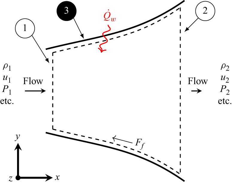


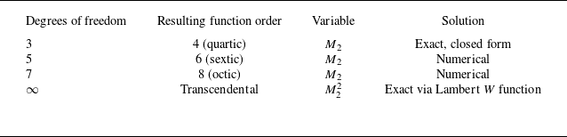





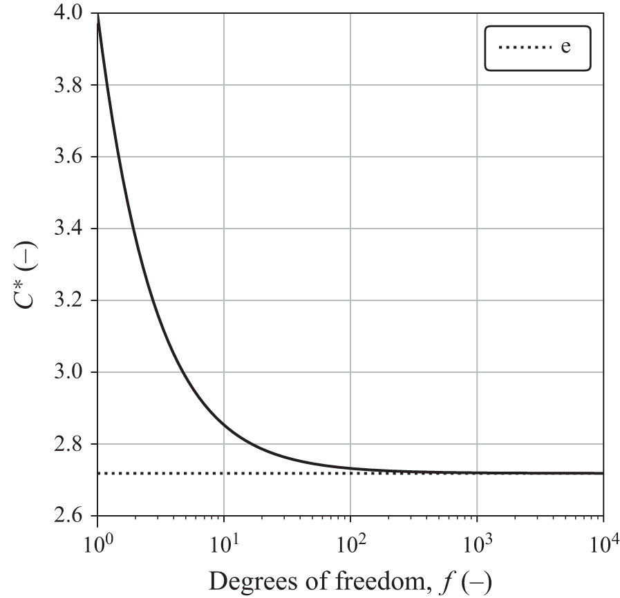


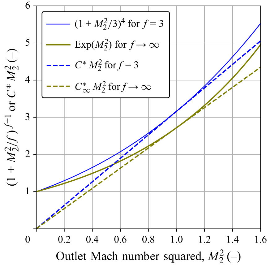


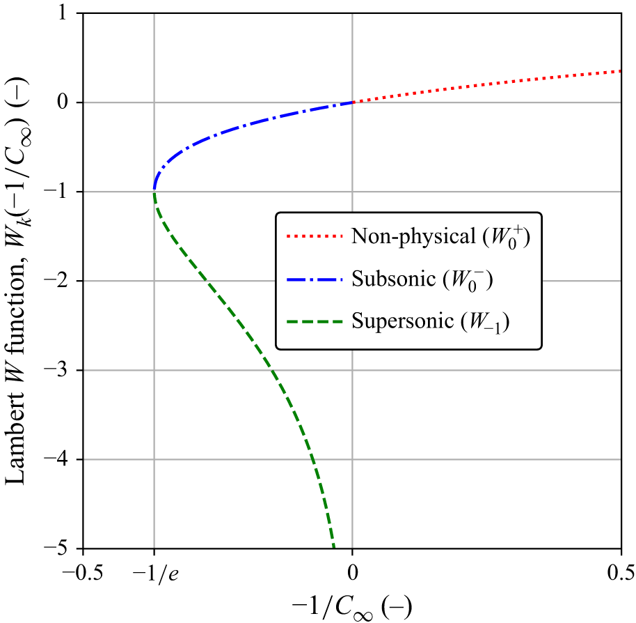


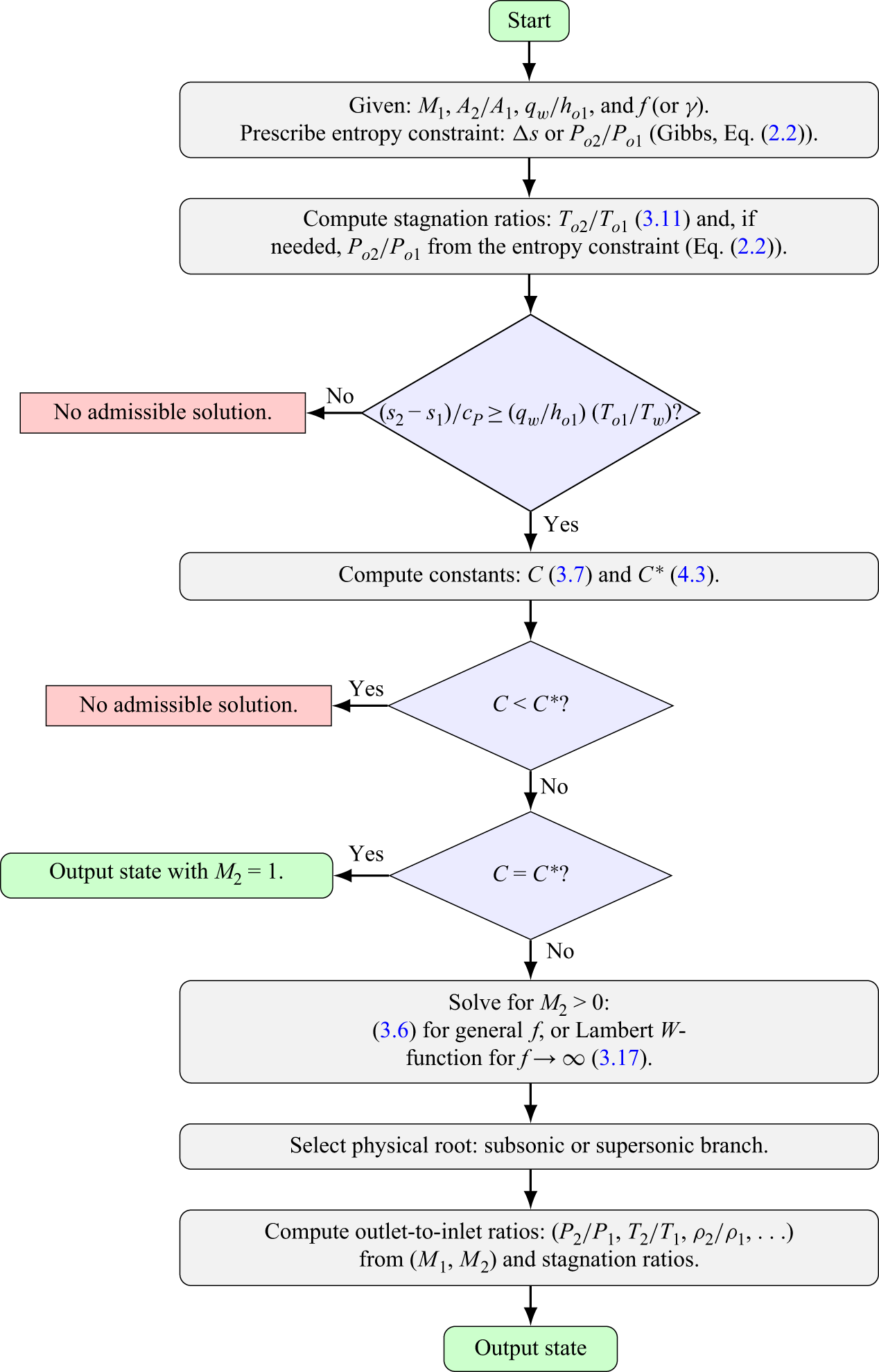
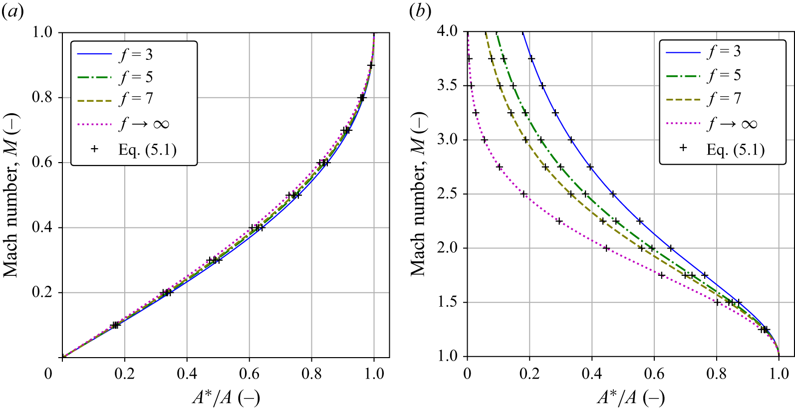


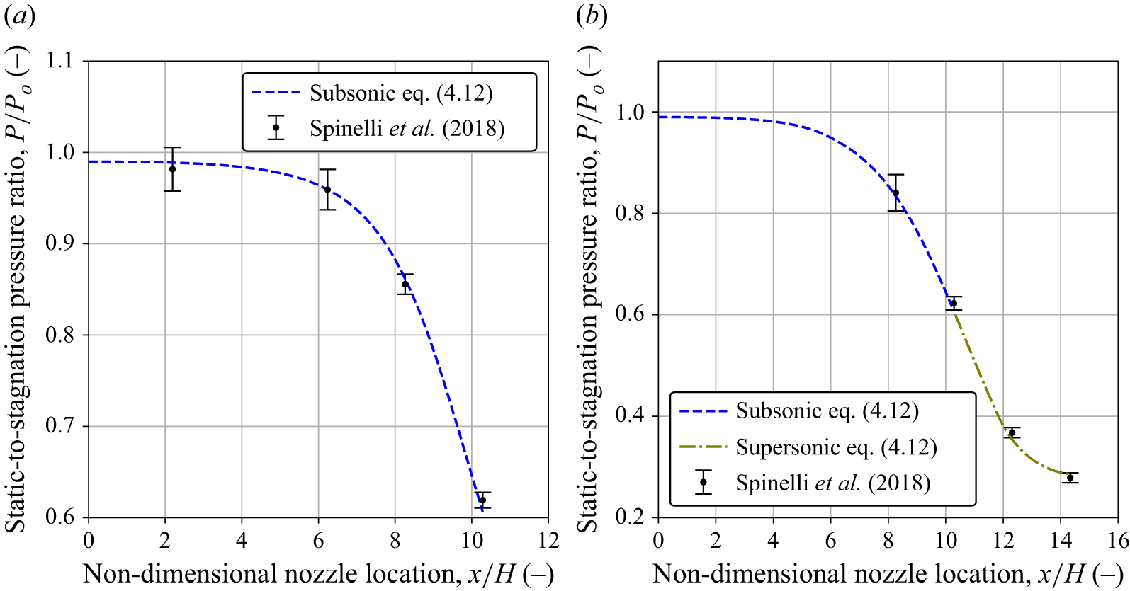

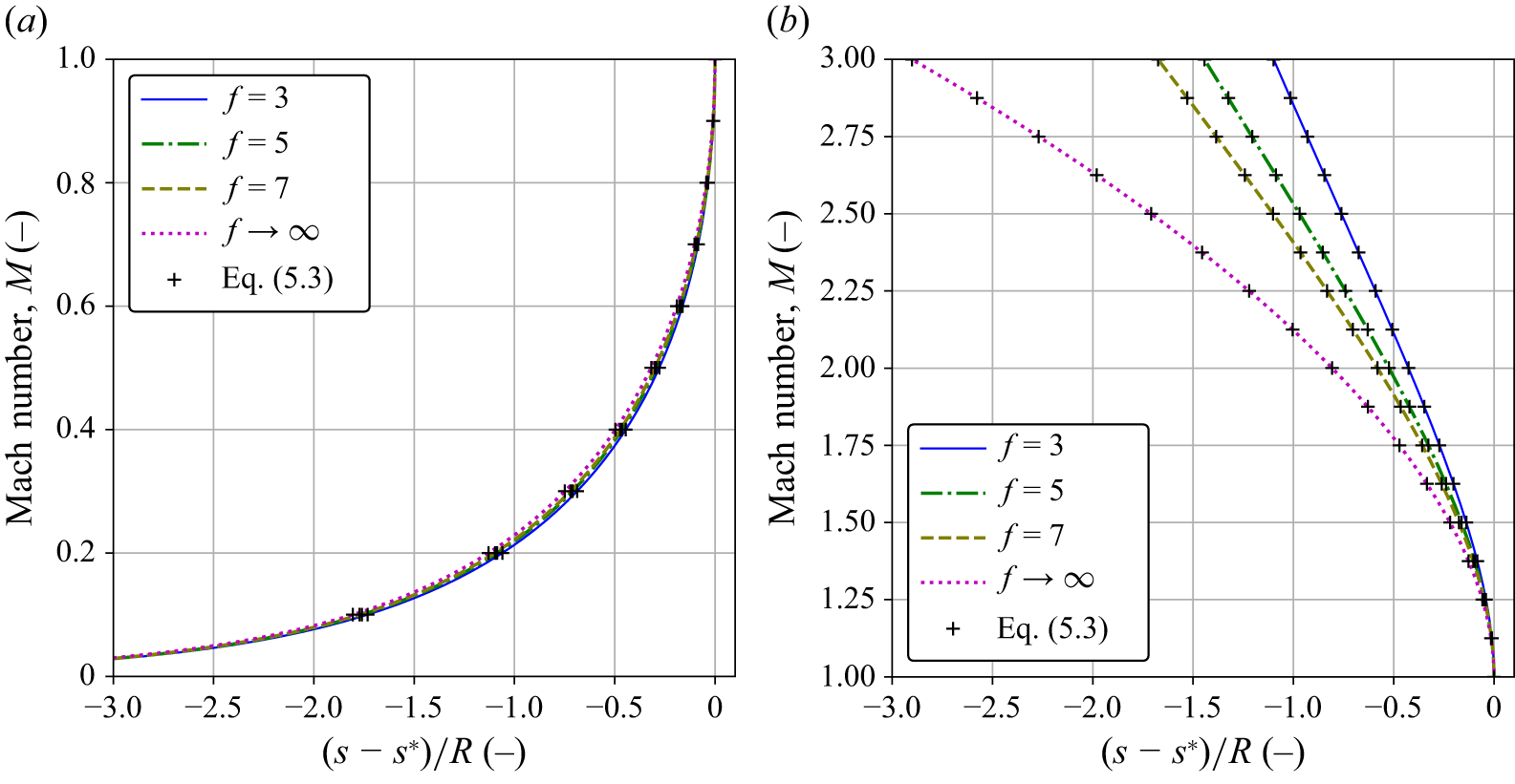


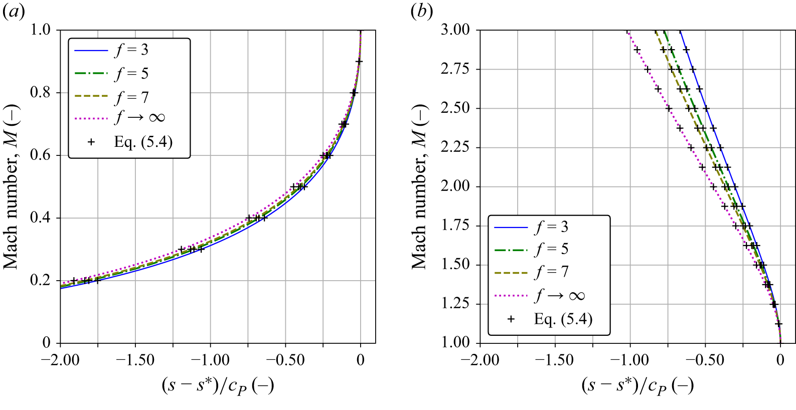


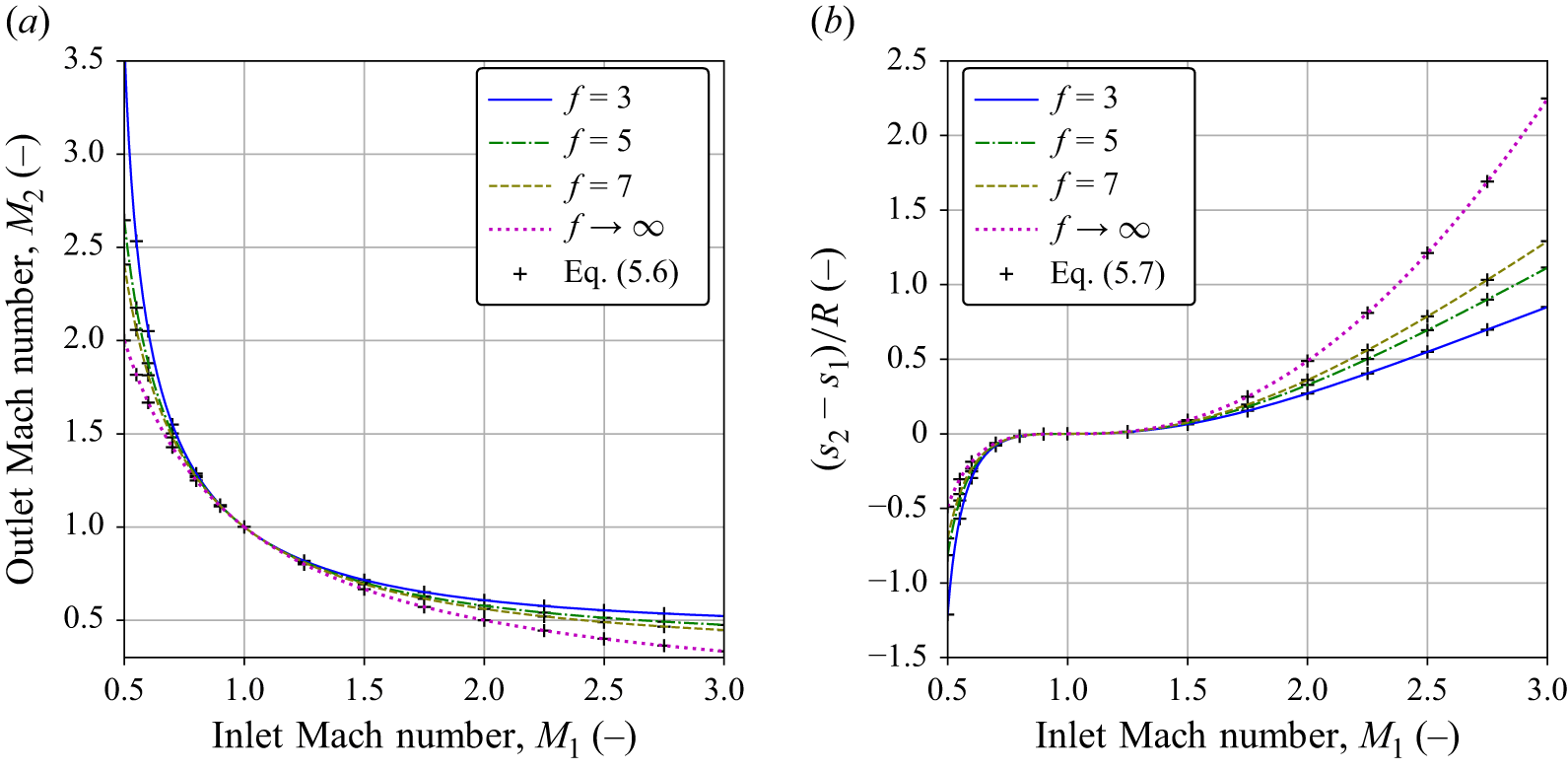


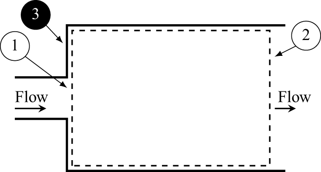
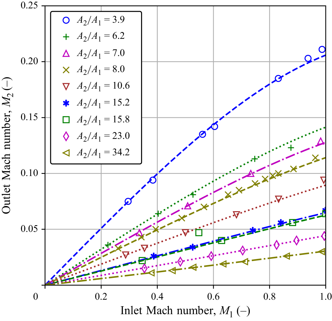


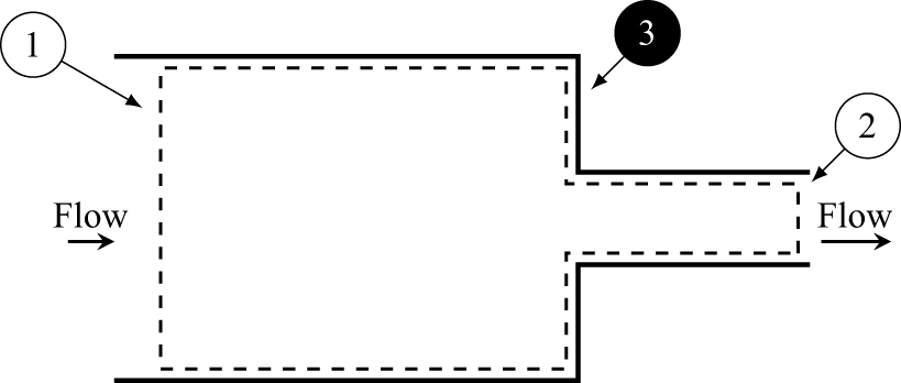
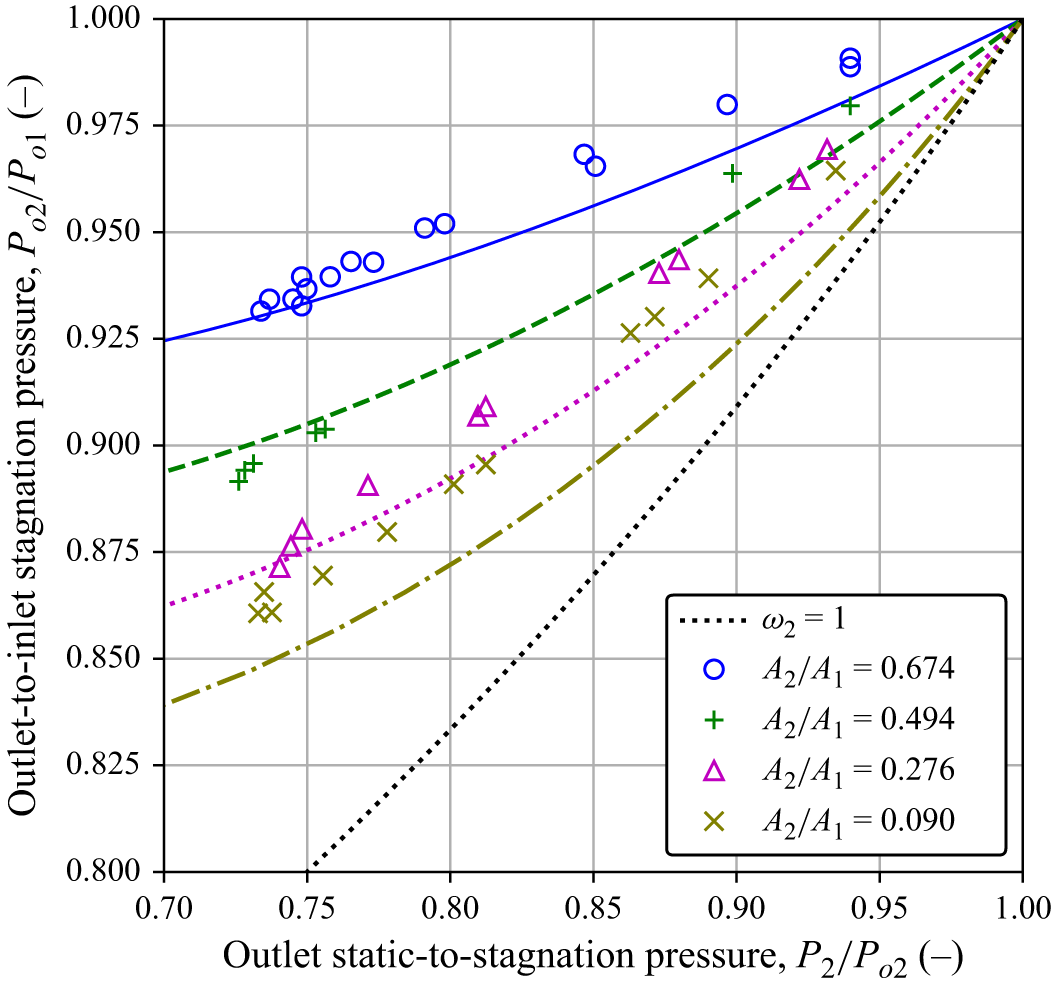


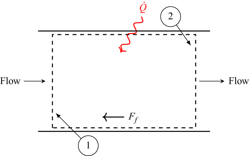
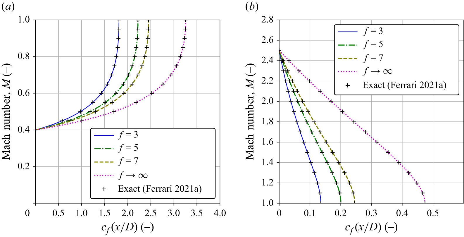


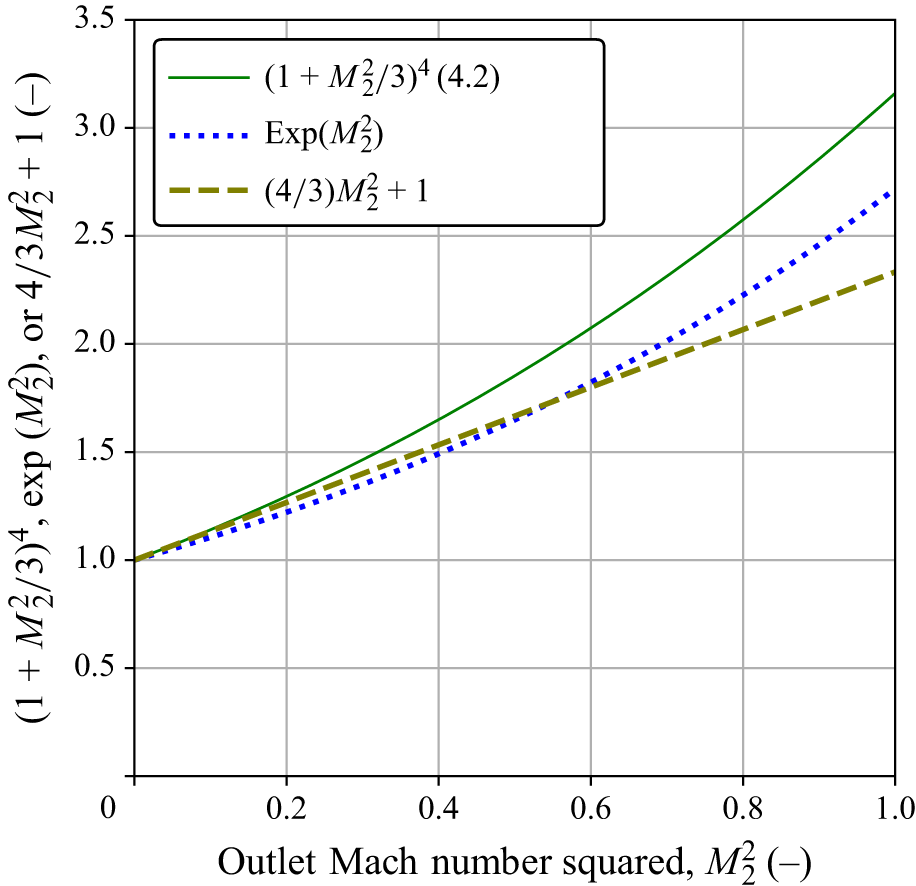


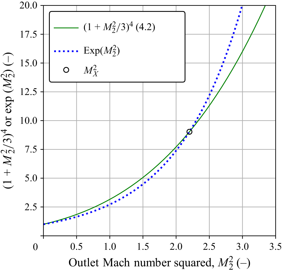


 Open access

