Introduction

Ice-core analyses yield remarkably detailed accounts of past climatic changes (e.g. Reference PetitPetit and others, 1999). the most widely used and high-resolution ice-core paleotemperature proxies are the isotopic compositions δ¹⁸O and δD of the ice. It is widely recognized that these δ values are sensitive not only to local ice-sheet temperature but also to source-region temperatures, because δ primarily measures fractional distillation of air-mass water content (e.g. Reference DansgaardDansgaard, 1964; Reference Aristarain, Jouzel and PourchetAristarain and others, 1986; Reference Jouzel, Russell, Suozzo, Koster, White and BroeckerJouzel and others, 1987, 1997; Reference BoyleBoyle, 1997; Reference CuffeyCuffey, 2000; Reference Hendricks, Paolo and CohenHendricks and others, 2000; Reference Vimeux, Masson, Delaygue, Jouzel, Petit and StiévenardVimeux and others, 2001). Also of primary importance is δ of marine source waters, δ_m. A zero-order relationship describing changes in δ values of the precipitate for ¹⁸O and D in terms of temperature shifts in the source region (ΔT_s) and at the location of deposition (ΔT_i), and source water shifts Δδ_m, is

(1)

where γ_s, γ_i and γ_m are constants with different values for each of the two isotope species. of principal interest is the temperature change at location of deposition, and thus a method for extracting ΔT_i from Equation (1) is sought. Marine composition changes can be estimated from oceanic records, but the source temperature change is more difficult to reconstruct. the deuterium excess, defined as d = δD– 8δ¹⁸O, has been proposed to provide this useful correction (Reference Johnsen, Dansgaard and WhiteJohnsen and others, 1989; Reference Petit, White, Young, Jouzel and KorotkevichPetit and others, 1991; Reference Vimeux, Masson, Delaygue, Jouzel, Petit and StiévenardVimeux and others, 2001), because fractionation accompanying evaporation is sensitive to temperature and relative humidity. General circulation model (GCM) calculations suggest that ocean surface temperature and relative humidity changes have been strongly correlated, so these effects are here lumped into one sensitivity b_s , so that

(2)

Combining Equations (1) and (2) yields the zero-order estimate for temperature changes at the ice-core site:

(3)

Thus the quantity γ_s/b_s emerges as a parameter of primary importance for ice-core paleoclimate reconstruction. All literature subsequent to the seminal work byReference Johnsen, Dansgaard and WhiteJohnsen and others (1989) considers d to be useful for paleoclimate correction specifically because of its dependence on source temperature. the dependence of d on source-region relative humidity and possibly wind speed are viewed as confounding factors.

In this paper, it is argued that this view needs to be broadened. In order to improve the use of d_i and γ_s/b_s in paleotemperature corrections, we here use an intermediate-complexity one-dimensional model of water-vapor transport to examine the factors that control δ¹⁸O and δD values in Antarctic precipitation (a modified version of the Reference Hendricks, Paolo and CohenHendricks and others (2000) model, which is a blend of earlier work by Reference ErikssonEriksson (1965) and Reference FisherFisher (1992)). We demonstrate that d of ice-sheet precipitation should vary as a function of many different sorts of climate changes in the oceanic source regions. Further, we demonstrate that most such changes cause anticorrelated variations of δD and d on the ice sheets. This indicates that d can be used to correct for changes in a number of source-region conditions (e.g. Reference Cuffey and VimeuxCuffey andVimeux, 2001) and thus has a more general utility for improving T_i reconstructions than has been previously recognized.

Model

The model (after Reference Hendricks, Paolo and CohenHendricks and others, 2000) was chosen in order to avoid some of the limitations of more commonly used simple Rayleigh models, which omit important physical mechanisms (evaporative recharge of air-mass water vapor; transport characteristics) and which do not explicitly incorporate climate data (e.g. values for P(θ) and E(θ)). GCMs are a superior tool for incorporating physical mechanisms (e.g. Reference Jouzel, Russell, Suozzo, Koster, White and BroeckerJouzel and others, 1987), but their complexity makes it difficult to isolate effects of changing single climate variables.

The essence of this model is an accurate accounting of the conservation of water vapor for each isotopic species along the transport path, in which both precipitation and evaporative recharge along the trajectory are incorporated. Climatological parameters are zonally averaged (Reference FisherFisher, 1992) and vapor transport is assumed to result entirely from advection by prevailing winds. We use the advective-transport case given by Reference Hendricks, Paolo and CohenHendricks and others (2000), for which the equation for the steady-state latitudinal gradient of airmass isotopic composition is

(4)

where θ is the local latitude, R_e is the radius of the Earth and w is the vertically integrated atmospheric water content. If w is expressed as water-column height, the precipitation P and evaporation E are given in units of ms^–1. the term Δ_p = δ_p – δ_a is the difference in isotopic composition between precipitate and atmospheric water vapor; Δ_e = δ_e – δ_a is the contrast between evaporative and ambient atmospheric values. Themean annual vapor-transport velocity v is related to the spatial gradient in atmospheric water content by

(5)

We use Equations (4) and (5) both directly from Reference Hendricks, Paolo and CohenHendricks and others (2000). Although modifications to these can be envisioned, adopting them directly from Reference Hendricks, Paolo and CohenHendricks and others (2000) is beneficial because the model behavior is already understood and analysis of it has been published. We do incorporate several important changes in the application of Equations (4) and (5), however. the transport path considered by Reference Hendricks, Paolo and CohenHendricks and others (2000) originates in the southern Pacific Ocean and traverses Antarctica from the west, crossing the Transantarctic Mountains. Recent GCM studies by Reference DelaygueDelaygue (2000) suggest that moisture following this path accounts for only ~20% of the mean annual precipitation at Vostok, while approximately 50% of the mean annual precipitation at Vostok comes from the southeastern Indian Ocean. We will consider both of these trajectories, and for convenience will refer to the transport path used by Reference Hendricks, Paolo and CohenHendricks and others (2000) as path 1and that originating in the Indian Ocean as path 2.

The isotopic composition of evaporation δ_e from the ocean surface is calculated using fractionation factors from Reference Horita and WesolowskiHorita andWesolowski (1994) and incorporating the parameterization of kinetic effects associated with vapor transport across a boundary layer between the ocean surface and the free atmosphere by Reference Merlivat and JouzelMerlivat and Jouzel (1979). In ice-covered regions, sublimation is the dominant recharge mechanism, and this is assumed to occur without additional fractionation. the evaporate in these regions is thus in isotopic equilibrium with local precipitate, and the effect of evaporation is to reduce the net accumulation.

The composition of precipitate is strongly temperature-dependent. In this study, we assume that only liquid is condensed at temperatures greater than –5˚C and that ice is the sole precipitate below –40˚C. Precipitate composition at intermediate temperature values is assumed to vary linearly. Isotopic fractionation during ice formation is calculated using equilibrium factors from Reference MajoubeMajoube (1971a, Reference Majoubeb) and assuming kinetic fractionation within the clouds, as in Reference Jouzel and MerlivatJouzel and Merlivat (1984). In nature, the altitude at which precipitate begins to form varies with the vertical temperature structure and atmospheric water content. Moreover, depending on the strength of convection, precipitate formation can occur over a significant vertical distance (and therefore temperature range). Rather than attempt to accurately parameterize these effects, we instead assume for simplicity that precipitation forms over the ocean at a temperature that is 6˚C cooler than the mean annual ocean surface temperature. Over the ice sheet, precipitation is assumed to form at the altitude corresponding to a similar cooling above the temperature inversion layer.

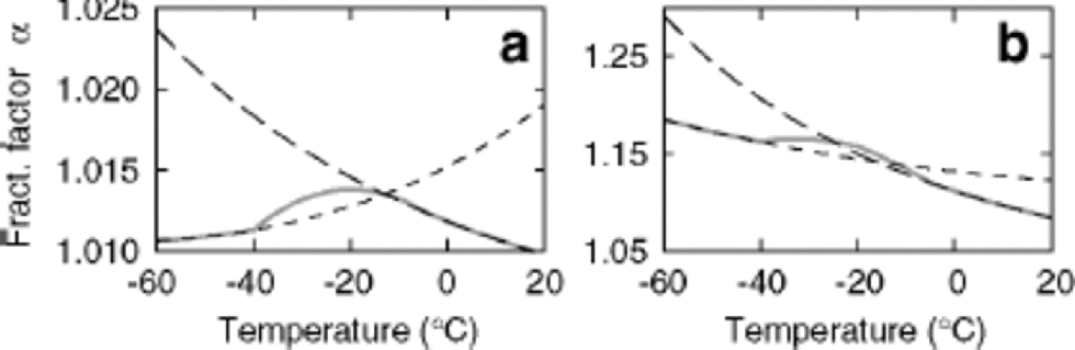
Fractionation factors for the liquid–vapor transition at low temperatures are poorly constrained. for this study, we have tuned the liquid–vapor deuterium fractionation factor at low temperatures in order to provide a better fit to field measurements of δD and d. Tuning against the data seems reasonable given the stability of excess measurements as discussed by Reference FisherFisher (1991), and this tuning is equivalent to the standard practice of tuning the cloud supersaturation (Reference Jouzel and MerlivatJouzel and Merlivat, 1984; Reference Johnsen, Dansgaard and WhiteJohnsen and others,1989). Figure 1 shows the fractionation factors used as a function of temperature (solidgrey line), along with the liquid–vapor fractionation factors of Reference Horita and WesolowskiHorita and Wesolowski (1994; long dashes) and the ice–vapor fractionation factors of Reference MajoubeMajoube (1971a, Reference Majoubeb; short dashes).

Fig. 1

Fractionation factors for δ ¹⁸O (a) and δ D(b) plotted as functions of temperature. Long dashes represent liquid– vapor fractionation factors of Reference Horita and WesolowskiHorita and Wesolowski (1994); short-dashed lines represent ice–vapor fractionation factors from Reference MajoubeMajoube (1971a, Reference Majoubeb). Kinetic effects are calculated as in Reference Jouzel and MerlivatJouzel and Merlivat (1984) using c = 1.00 and F = 0.007. These values are within the range suggested by Reference Johnsen, Dansgaard and WhiteJohnsen and others (1989). the liquid–vapor fractionation factor for δ D is tuned to provide the best fit to field data from Qin and others (1994) as discussed in the text.

We have found through experimentation that results presented in this paper are not at all sensitive to the specifics of the tuning. Any tuning that yields a δD and d that co-vary according to the measured relationship gives similar results.

Primary weaknesses of the model as a representation of nature are as follows. Because of the one-dimensional formulation of this model, values for atmospheric parameters represent vertical averages (as in the case of the transport velocity) or integrals (such as the atmospheric water content). Vertical structures in the atmosphere are therefore not considered. This is likely to have the greatest effect on isotope composition near the ocean–ice boundary, where there is significant vertical stratification within the atmosphere. In addition, this model considers only advective transport of water vapor. Eddy diffusion is likely to be an important transport mechanism, especially in the interior regions of Antarctica. It should be noted, however, that attempts to model δ values using purely diffusive transport produced spatial distributions that poorly matched field measurements.

Values for the zonal averages of precipitation P(θ), evaporation E (θ), water content w(θ) and surface temperature T_s(θ) are those used by Reference Hendricks, Paolo and CohenHendricks and others (2000) as follows. Their estimates of P (θ) and E(θ) are based primarily on the U.S. National Centers for Environmental Prediction (NCEP) re-analysis for years 1979–97 (Reference KalnayKalnay and others, 1996). Along path 1, values of P (θ) and E(θ) over Antarctica were modified to better match estimates by Reference Giovinetto, Bromwich and WendlerGiovinetto and others (1992) and Reference Giovinetto and BentleyGiovinetto and Bentley (1985), respectively. These values were used to allow direct comparison with model results from Reference Hendricks, Paolo and CohenHendricks and others (2000). Along path 2, net accumulation rates taken from the Reference HuybrechtsHuybrechts (1990) application of Reference Fortuin and OerlemansFortuin and Oerlemans (1990) are used in place of separate P and E estimates. Values for w(θ) are based on a simple model assuming 75% relative humidity and a lapse rate of –6^˚C km^–1 over the mid-latitudes; the decreased atmospheric height over the Antarctic plateau and the positive lapse rate of the surface inversion layer are also considered. Sea surface temperatures are also from NCEP data, while Antarctic surface temperatures are from Qin and others (1994). the relative humidity h(θ) is assumed to be linearly related to the surface temperature; values produced by this method are similar to those from Reference BroeckerBroecker (1997). Surface waters for most model runs are assigned δ¹⁸O and δD values of 0‰.

Integration of Equation (4) begins at a latitude of 43˚ S, just south of the location where evaporation and precipitation rates are equal (i.e. the southern edge of the Equatorial evaporation-dominated zone). Thus the physical counter part for the model’s initial condition is the average atmospheric δ composition in this geographic region where there is no local net source of air-mass recharge. on Earth, this value is determined by conditions in the ``desert belt’’ between ~20˚ S and this location. Important controls are the composition of evaporation and the amount and temperature of convective precipitation. In the present study we do not try to model this explicitly; this will be investigated in future work (see also Reference Jouzel and KosterJouzel and Koster, 1996). Because conditions in the desert belt are not modeled here, initial atmospheric deuterium excess values at the low-latitude limit are chosen explicitly and adjusted as part of model calibration. In the following model runs, the initial deuterium excess values are set to d_p = 4‰ for path 1 and d_p = 5‰ for path 2. These numbers are consistent with data (Reference Jouzel, Russell, Suozzo, Koster, White and BroeckerJouzel and others, 1987).

Integration continues to the location where minimum values for T_s, w, P –E and δ_p are reached. This condition is met near the center of the Antarctic Plateau near Vostok (78˚28’ S, 106˚48’ E) rather than at the true geographic South Pole, and thus we adopt the shifted coordinate system of Reference Hendricks, Paolo and CohenHendricks and others (2000) in whichVostok is defined as the model origin. Except where noted, the atmospheric δ¹⁸ _a O at the low-latitude limit is set to that of the evaporate at that location, as determined by surface temperature and humidity conditions (Reference Merlivat and JouzelMerlivat andJouzel, 1979).

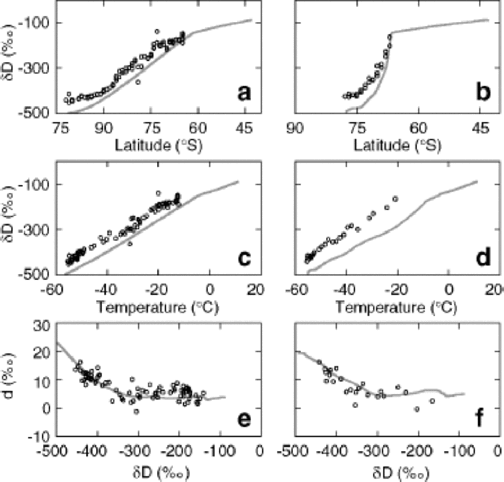
Modeled δD values for precipitation along paths 1 and 2 are shown as functions of latitude (Fig. 2a and b) and temperature (Fig. 2c and d). Although modeled values along both trajectories show values below those recorded by Qin and others (1994), the model reproduces the general trends of the data. We have chosen not to remove this difference by tuning of the climate variables because a number of poorly quantified factors may contribute. Temperature values used in calculating δ_p values are based on estimates of mean annual temperature. However, the seasonal and weekly timing of precipitation are likely biased to favor precipitation when air masses are warmer than average, which means effective temperatures of condensation should be higher and fractionations smaller. Similarly, the effective mean altitude (and therefore temperature) at which precipitation occurs is poorly known. Finally, calculated d values are slightly dependent on the initial latitude, and changing the starting point of integration shifts the entire curve slightly left and right. Figure 2e and f show the deuterium excess d_p of the precipitation plotted as a function of δD_p. Because the deuterium excess is a linear combination of δ¹⁸O and δD, any offsets introduced by the parameterizations of surface and cloud temperatures or by the choice of initial latitude will be effectively cancelled, as both δ¹⁸O and δD will be affected similarly. for this reason, the relationship between d and δD is more useful in constraining the isotopic model. Accordingly, we have tuned the deuterium fractionation factor for the liquid–vapor transition to optimize the match between model and field values of d and δD as described above.

Fig. 2

Model results using values for P , E , T_s and w from Reference Hendricks, Paolo and CohenHendricks and others (2000). Modeled δ D values for precipitation along paths 1 and 2 are shown as functions of latitude (a, b) and surface temperature (c, d). the deuterium excess d = 8 δ ¹⁸O of the precipitation is plotted against δ D along paths 1 and 2 in (e) and (f). Circles represent field measurements by Qin and others (1994).

Thus, because we have not optimized the δ–latitude relationship, if we wish to examine the model isotopic change at a specific location such as Vostok, we define this as the change at the latitude for which the standard model δD value is the same as that observed for Vostok. In other words, we use the net isotopic distillation as the best measure of location.

Numerical Experiments

To illustrate the effects of source-region climate changes on precipitation isotopes over the ice sheet, numerical experiments are performed in which adjustments of initial conditions and of climatic variables in the oceanic region of the model domain are imposed and compared to the standard case. of particular interest here are the simultaneous changes in ΔδD and Δd resulting from the imposed climate change; the ratio ΔδD/Δd is a generalized analogue of the ratio γ_s/b_s from Equation (3).

In all but one of the experiments that follow, conditions over the ice sheet are held constant, and thus these controlled experiments are not intended to realistically imitate natural climate changes. It is very unlikely, for example, that in nature there would be climatic changes over the oceans around the ice sheet that are not accompanied by any change over the ice sheet at all. Thus, quantitative results from our experiments are expected to differ from results of GCMs or other models that actually calculate the climate change in a physically realistic fashion as a function of forcings.

Experiments I

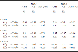
We first examine the model response to very simple changes in temperature, relative humidity and marine isotopic composition, the traditionally recognized controls on d of ice-sheet precipitation (Reference Petit, White, Young, Jouzel and KorotkevichPetit and others, 1991; Reference Vimeux, Masson, Delaygue, Jouzel, Petit and StiévenardVimeux and others, 2001). Values for ΔδD, Δd and ΔδD/Δd for these initial model runs are shown in Table 1. These changes are given for two locations, corresponding to the latitudes at which base-model δD values are δD₀ = –250‰ and δD₀ = –450‰. the effects of increasing marine δ¹⁸O by 1‰ and δD by 8‰ (and therefore maintaining the deuterium excess values of the base models) are shown in Figure 3a and b (solid black line). Changes for both paths are similar. Note that the excess changes at Δd{–₄₅₀} = –3.0 for both paths are nearly identical to the estimate using the Goddard Institute of Space Studies (GISS) GCM(Reference Vimeux, Masson, Delaygue, Jouzel, Petit and StiévenardVimeux and others, 2001).

Table 1.

Model results for Experiments I. Case 1: marine δ ¹⁸O increased by 1 ‰, marine δd increased by 8 ‰ . Case 2: ocean surface cooled as discussed in the text. Case 3: global relative humidity decreased by 5%

We next investigate the effects of reducing the surface temperature T_s of the ocean. to avoid discontinuities in the temperature or the temperature gradient, and to avoid

Fig. 3

Model results for Experiments I. Shown are results for (1) increasing the marine δ ¹⁸O by 1 ‰ and the marine δd by 8 ‰ (solid black line), (2) cooling the ocean surface as discussed in the text (long dashes), and (3) decreasing the global relative humidity by 5‰ Standard model values as shown in Figure 2e and f (solid grey line), and field measurements by Qin and others (1994) (circles) are shown for comparison. (a) Path 1. (b) Path 2.

changing the temperature over the ice sheet, a cooling (magnitude 5˚C) is imposed at the low-latitude integration limit, and the magnitude of cooling is reduced linearly to the Antarctic coastline (latitude θ = 61.5˚ S for path 1 and θ = 66.5³S for path 2), where no cooling occurs. the water content w is scaled by the surface temperature to preserve the relationship between w and temperature (thus w(T_s) = w(T_s,₀), where T_s,₀ and T_s are the surface temperature before and after the temperature shift), but no changes are made to P(θ) or E(θ). Note that any scenario that results in the cooling of coastal waters (including those that change the continental temperature structure) also requires adjustment of the extent of sea-ice cover. Such adjustments are simple to implement numerically but result in secondary δ changes that are difficult to separate from the signal of primary interest.

The temperature dependence of the fractionation factors implies they are higher at the lower temperatures than in the standard case. the effect of this is to increase distillation and hence decrease δD at a given latitude. However, this effect is overcompensated by the reduction in distillation due to the reduced gradient dw/dθ associated with the reduced temperature gradient (the transport velocity v must be higher to produce the same P –E given the reduced gradient; the faster transport then means there is less fractional reduction of air-mass water content due to P). Thus distillation is reduced and δD values increased (consistent with the basic temperature-gradient interpretation of the Rayleigh model) with similar magnitude for both paths (Table1; Fig. 3a and b, long dashes). the excess decreases along both paths, producing ΔδD/Δd values that are comparable to those for the marine composition change. the magnitude of the decreases in d (–2.5 to –4.5 for a temperature decrease of 0–5˚C) are similar to the b_s values calculated by Rayleigh models and the GISS GCM (Reference Petit, White, Young, Jouzel and KorotkevichPetit and others, 1991; Reference Vimeux, Masson, Delaygue, Jouzel, Petit and StiévenardVimeux and others, 2001). Below we will revisit the effects of temperature change, allowing scaling factors for P and E.

A global 5% reduction in relative humidity (Table 1; Fig. 3a and b, short dashes) yields ΔδD and Δd values that are of opposite sign compared to those in the previous two scenarios (consistent with Reference Petit, White, Young, Jouzel and KorotkevichPetit and others, 1991). As humidity values approach 100%, evaporation more closely approximates an equilibrium process. In contrast, the modeled reduction in humidity values strengthens the kinetic effects, and results in increased deuterium excess values.

Experiments II

Other source-region changes can occur that will also affect the d of ice-sheet precipitation. This is a consequence of the fractional nature of distillation; for an air mass that is not being recharged by evaporation (considered for simplicity), a differential change in either δj (where j =¹⁸O or D) due to a differential change in water content is

(6)

Here αj is the appropriate fractionation factor for the given isotopic species. This can be derived by substituting Equation (5) into Equation (4), and setting E = 0 (also see Reference Merlivat and JouzelMerlivat and Jouzel, 1979; Reference Johnsen, Dansgaard and WhiteJohnsen and others, 1989). Thus, regardless of its initial value, d will evolve as a function of (α_D – 1)(1+ δD) – 8(α18 – 1)(1 + δ¹⁸O). Any factor that affects the covariation of α’s and δ’s along the vapor-transport path will cause some change of d over the ice sheet. Most clearly, if α are strictly functions of temperature, then any climatic changes that alter the temperature at which a given δ is attained will inevitably cause a change in the excess. This means that also of importance are all of the source-region variables that play a role in the advective Equation (4), including the recharge fraction E(θ)/w(θ), precipitation P(θ), the source-region geography (i.e. where P = E, or the location of zero net divergence), and the δ¹⁸O and δD values at the location of zero net divergence. These initial d values potentially depend on both the magnitude of transport relative to E–P in the desert belt and the effective altitude of condensation (or the strength of convection within this region). We will therefore investigate a number of modeling scenarios of changes to either the hydrological conditions along the transport paths or the initial atmospheric δ values.

The simplest possible scenario is a change of initial δ values without any other source-region or path changes. Increasing initial δ¹⁸O by +1.0‰ without any change of the excess (i.e. by also increasing the initial δD by 8‰) causes a measurable change of d over the ice sheet without any change in the excess of evaporation (Table 2; Fig 4a and b, solid black line). If we impose a change in only the initial excess (i.e. a change in δD with no corresponding change of δ¹⁸O), the signal generated over the ice sheet is significantly reduced compared to the initial signal (Table 2; Fig. 4a and b, long dashes). These two calculations indicate that the excess signal over the ice sheet is generally more sensitive to the low-latitude δ¹⁸O than to the low-latitude excess.

Fig. 4

Model results for Experiments II. (a, b) (1) Initial δ ¹⁸O increased by 1.0 ‰ (solid black line). (2) Initial excess d doubled (long dashes). (3) Starting point of integration shifted halfway to the ocean edge (short dashes). (c, d) (4) Precipitation scenario A (solid black line). (5) Precipitation scenario B (dashed line). (e) (6) Global 50% reduction in evaporation (solid black line). (7) P(θ) = 1.1E(θ) (dashed line). Standard model values as shown in Figure 2e and f (solid grey line), and field measurements by Qin and others (1994) (circles) are shown for comparison. Results for path 1 are shown in (a), (c) and (e); results for path 2 are shown in (b) and (d).

Table 2.

Model results for Experiments II. Case 1: Initial δ ¹⁸O increased by 1.0 ‰ . Case 2: Initial excess d doubled. Case 3: Starting point of integration shifted halfway to ocean edge. Case 4: Precipitation scenario A (see text). Case 5: Precipitation scenario B (see text). Case 6: Global 50% reduction in evaporation. Case 7: P(θ) = 1.1E(θ)

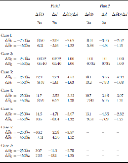
Another simple source-region change is a geographic shift of the low-latitude boundary (location of zero net divergence). If we shift the latitude at which the model integration begins (but do not modify other model parameters), changes in both δD and d result over the ice sheet (Table 2; Fig. 4a and b, short dashes). Moving the boundary closer to the ice sheet reduces net distillation, increasing the δD and δ¹⁸O. Because the δ values increase at a given temperature along the transport path, a corresponding decrease of the excess inevitably results.

All three of these examples are independent of changes in climate or evaporate along the transport trajectory. the following calculations illustrate effects of changing hydrologic characteristics in the oceanic part of the trajectory.

First, a temperature change that is zero at the ice-sheet edge and increases linearly to the low-latitude boundary is examined. In the previous discussion of such a shift (Experiments I) values for the evaporation E(θ) and precipitation P(θ) were unchanged, implying that the change in the meridional w gradient was compensated by changes in transport rate. Generally this is unrealistic, and a reduction of precipitation is expected to accompany a reduction in meridional temperature gradient. In this subsection, we scale the evaporation with the surface temperature change such that where T_s and T_s,₀ are the surface temperatures before and after the temperature shift, and scale the precipitation by two different relations. In the first, which we will refer to as scenario A, the precipitation is scaled as

(7)

where v₀(θ) is the transport velocity field given by Equation (5). (Inspection of Equation (5) shows that P and v cannot be redefined simultaneously.) In scenario B, the precipitation is scaled by

(8)

where T_c and T_c,₀ are the cloud temperatures before and after the temperature shift. the additional factor in Equation (8) is included as an analogue to a reduction of transport velocity accompanying the decreased temperature gradient, as Table 2 and Figure 4c and d give results for these calculations (precipitation scenario A: solid black line; precipitation scenario B: dashed line). for both scenarios, net distillation is decreased (increasing δD) and the corresponding decrease of excess is again clearly seen.

Finally, we show calculations for which E(θ) and P(θ) are scaled independently, and without any change in temperatures. These modeling scenarios are calculated for path 1 only, as net accumulation data are used for path 2 (rather than calculating the accumulation from separate estimates of P and E). A global 50% reduction in evaporation produces increased net distillation (lower δD) because of the reduced importance of recharge by isotopically heavy waters (Table 2; Fig. 4e, solid black line), and a similar anticorrelated change in excess (because lower δ are attained at a given temperature). to investigate the effects of a climate with exceptionally vigorous recharge, we scale the precipitation to the evaporation by P(θ) = 1.1E(θ). As one would expect, changes in isotopic composition are opposite to the previous case, showing increased δD values and decreased d (Table 2; Fig. 4e, dashed line). Again, changes in δD and d are anticorrelated.

Each of the preceding four climate scenarios results in correlative changes in both d and δD at Vostok. Despite the large range in ΔδD (–10.2 to +30.7 and –7.51 to +22.5 for δD₀ = –250‰ and –450‰, respectively) and Δd (–11.0 to +2.58 and –18.1 to +4.96), values for the ratio of these quantities are surprisingly uniform, ranging between –2.78 and –3.97 at δD₀ = –250, and –1.25 and –1.52 for δD₀ = –450‰. This is a direct result of Equation (6) and the fact that the fractionation factors are only functions of temperature.

Concluding Discussion

Although we recognize that the modeling experiments presented in this study are physically unrealistic (because we modify certain climatologic variables without calculating changes to others in a physically based fashion; and because the isotopic model is simple), we believe that the results provide an informative, if qualitative, perspective on controls of polar ice-sheet deuterium excess. Most importantly, these calculations indicate that the deuterium excess responds to a wide variety of climatologic factors in addition to the composition of oceanic evaporate. This complicates interpretations of d time series in terms of source-region temperature and relative humidity. However, it is important to keep in mind that the sorts of source-region changes we have examined very likely correlate strongly with source-region temperature. Regardless of implications for reconstruction of source-region climate, a clear result of our calculations is that a wide variety of source-region changes cause anticorrelated changes of δD and d over the ice sheets, with a ratio ΔδD/Δd generally in the range –1.4 to –3.5. the d may therefore be more useful than is presently recognized as a tool for correcting ice-core δD records for source-region effects. It is very important to ask what this result implies for interpretation of the Vostok deuterium record (Reference Vimeux, Masson, Jouzel, Stiévenardand and PetitVimeux and others, 1999). Answering this question is, however, beyond the scope of the simple model employed here. Experiments with rigorous climate models, such as GCMs with isotopic tracers, will be most useful for this inquiry. Moreover, such models are absolutely necessary for estimating quantitatively reliable values for the covariation factor ΔδD/Δδ, because it is unrealistic to prescribe source-region climate changes that have no correlated changes over the ice sheets, and because the nature of P, E and transport changes should be calculated rather than prescribed.