


1. Introduction
Thin liquid films interacting with gas flows are frequently encountered in engineering applications and in nature. The dynamics of these systems have a significant impact on the performance of industrial equipment such as evaporators, condensers and chemical reactors (Hanratty & Engen Reference Hanratty and Engen1957; McCready & Hanratty Reference McCready and Hanratty1985), as well as in processes like coating (Buchlin Reference Buchlin1997) or arc welding (Berghmans Reference Berghmans1972). Using direct numerical simulations, Lombardi, De Angelis & Banerjee (Reference Lombardi, De Angelis and Banerjee1996) and De Angelis, Lombardi & Banerjee (Reference De Angelis, Lombardi and Banerjee1997) have shown that, in some configurations, the large difference of scales in the dynamics of the two flows allows for treating the liquid phase as a ‘rigid’ boundary for the gas phase, thus decoupling their dynamics. However, this assumption is only valid when the interfacial deformations (waves) are confined to the viscous sublayer of the gas (Rosskamp, Willmann & Wittig Reference Rosskamp, Willmann and Wittig1998). When this condition is not met, as in most configurations of practical interest, understanding the gas–liquid interaction is crucial to improving the performance of the two-phase system. Examples of configurations with strongly coupled gas-interface interaction are the cavity flow produced by a jet impinging on a liquid bath (Ojiako et al. Reference Ojiako, Cimpeanu, Bandulasena, Smith and Tseluiko2020) or the waves in falling liquid films subject to concurrent or counter-current laminar gas flows (Dietze & Ruyer-Quil Reference Dietze and Ruyer-Quil2013).
A third example, which is the focus of this work, is the jet-wiping process. It consists in using impinging planar gas jets to control the thickness of a thin film dragged by an upward-moving substrate. The process is widely used in hot-dip galvanizing because it allows for a precise and contactless control of the amount of zinc deposited on a steel substrate for corrosion protection. Simplified analytical models to predict the average coating thickness downstream jet wiping have been proposed by Thornton & Graff (Reference Thornton and Graff1976), Buchlin (Reference Buchlin1997) and Yoneda (Reference Yoneda1993), while early stability analyses based on the Orr–Sommerfeld problem (Tuck Reference Tuck1983), and integral models (Tu & Ellen Reference Tu and Ellen1986) have concluded that the configuration is neutrally stable. This result was later confirmed by Hocking et al. (Reference Hocking, Sweatman, Fitt and Breward2011) using quasisteady models also accounting for the gas-induced shear stress at the interface, and by Ivanova et al. (Reference Ivanova, Pino, Scheid and Mendez2023) and Barreiro-Villaverde, Gosset & Mendez (Reference Barreiro-Villaverde, Gosset and Mendez2021) who investigated the dynamics of waves on thin films dragged by a solid wall. Nevertheless, all these works assumed a stationary jet flow or no jet flow. Experimental and numerical investigations by Gosset (Reference Gosset2007) and Myrillas et al. (Reference Myrillas, Rambaud, Mataigne, Anderhuber, Gardin, Vincent and Buchlin2013), later extended by Gosset, Mendez & Buchlin (Reference Gosset, Mendez and Buchlin2019) and Mendez, Gosset & Buchlin (Reference Mendez, Gosset and Buchlin2019b), have shown that the jet wiping is intrinsically unstable and characterized by a strong coupling between the gas and liquid phases, resulting in large oscillations of the impinging jet combined with large waves in the liquid film. This instability produces non-uniformities (long-wavelength undulations) on the final coating, limiting the quality of products requiring high surface finish, such as those for the automotive industry.
Besides the industrial relevance, understanding the origin of the jet-wiping instability remains a fundamental and unsolved problem in fluid dynamics, especially because this flow configuration remains inaccessible to comprehensive experimental and numerical investigations in industrial conditions. The link between the unsteadiness of the jet flow and the response of the coating layer was analysed via integral boundary layer (IBL) models introduced by Kapitza (Reference Kapitza1948) and Shkadov (Reference Shkadov1970) in a quasisteady formalism by Johnstone et al. (Reference Johnstone, Kosasih, Phan, Dixon and Renshaw2019) and using self-similar and weighted integral boundary layer (WIBL) models (Ruyer-Quil & Manneville Reference Ruyer-Quil and Manneville2000, Reference Ruyer-Quil and Manneville2002) by Mendez et al. (Reference Mendez, Gosset, Scheid, Balabane and Buchlin2021). These works have allowed for deriving the dimensionless transfer function of the coating film against harmonic and non-harmonic jet oscillations and/or pulsations, showing that a narrow range of high sensitivity exists in the dimensionless frequency domain obtained by scaling the problem using time and length scales built from the liquid film properties. This result is in agreement with the findings of Lunz & Howell (Reference Lunz and Howell2018) for liquid coatings on inclined planes.
Nevertheless, the main limitation of these theoretical works is that they are based on a one-way coupling formulation in which synthetic perturbations are introduced into the film to analyse its receptivity. More advanced two-way coupling requires more sophisticated simulations and modelling approaches. Examples of such two-way coupling approaches are proposed by Lavalle et al. (Reference Lavalle, Vila, Blanchard, Laurent and Charru2015), who combined an integral film model with a full Navier–Stokes solver for the shearing laminar gas flow; Miao, Hendrickson & Liu (Reference Miao, Hendrickson and Liu2017), who proposed a similar solution using an immersed boundary (IB) method; and Ojiako et al. (Reference Ojiako, Cimpeanu, Bandulasena, Smith and Tseluiko2020), who coupled a single-phase solver with a film model for a gas jet impinging on a liquid bath to obtain the stationary shape of the gas–liquid interface. However, the use of such kind of ‘hybrid’ approaches for the jet-wiping problem remains an open challenge due to the large difference in the scales of the liquid and the (turbulent) gas flow, especially in the wiping conditions encountered in galvanization.
Alternative solutions using state-of-the-art methods from two-phase computational fluid dynamics (CFD) face the same problems. The most common approach is to combine the volume of fluid (VOF) method and large-eddy simulation (LES) modelling for gas jet turbulence. This was the method used by Myrillas et al. (Reference Myrillas, Rambaud, Mataigne, Anderhuber, Gardin, Vincent and Buchlin2013) and Barreiro-Villaverde et al. (Reference Barreiro-Villaverde, Gosset and Mendez2021) for the three-dimensional (3-D) simulations reproducing the wiping of highly viscous fluids in the experiments of Gosset (Reference Gosset2007), Gosset et al. (Reference Gosset, Mendez and Buchlin2019) and Mendez et al. (Reference Mendez, Gosset and Buchlin2019b), which allowed for the first description of the wiping instability. However, these investigations focused on conditions that are extremely far from the ones encountered in galvanizing conditions, as further discussed in the following section. To the best of the authors’ knowledge, high-fidelity simulations of the process in galvanizing conditions are limited to two-dimensional (2-D) computations (Pfeiler et al. Reference Pfeiler, Eßl, Reiss, Riener, Angeli and Kharicha2017b,Reference Pfeiler, Eßl, Reiss, Ecker, Riener and Angelia) while the only attempt to reproduce it in three dimensions is due to Aniszewski et al. (Reference Aniszewski, Saade, Zaleski and Popinet2020). Despite the significant amount of computational resources ( ${\approx }5\times 10^{5}$ central processing unit (CPU) hours) and the use of highly optimized grid-adapting code such as Basilisk (Popinet Reference Popinet2015), the simulations in Aniszewski et al. (Reference Aniszewski, Saade, Zaleski and Popinet2020) only covered a few instants of the initial stage of the interaction, when the jet first impinges on the liquid film and begins to produce the wiping meniscus. Extending those simulations to achieve established wiping conditions was not feasible.
Considering the prohibitive computational costs reported in Aniszewski et al. (Reference Aniszewski, Saade, Zaleski and Popinet2020), the full high-fidelity simulation of the jet wiping in galvanizing conditions is likely going to remain unfeasible in the near future. Therefore, an important open question is the extent to which the results obtained for highly viscous fluids in Barreiro-Villaverde et al. (Reference Barreiro-Villaverde, Gosset and Mendez2021), Gosset et al. (Reference Gosset, Mendez and Buchlin2019) and Mendez et al. (Reference Mendez, Gosset and Buchlin2019b) are relevant for the much broader spectra of wiping conditions encountered in industry. This article is an attempt to tackle this question. Specifically, we complement the work in Barreiro-Villaverde et al. (Reference Barreiro-Villaverde, Gosset and Mendez2021) with the investigation of the wiping process in conditions that are closer to the industrial ones. Although far from achieving full dynamic similarity, as discussed in the following section, the investigated conditions cover a completely different wiping regime than what was previously reported in the literature. Therefore, the results give an insight into the dynamics and the scaling of the jet-wiping instability and perhaps enable an educated extrapolation. Moreover, we use the CFD results to examine the theoretical foundations of the classic jet-wiping models.
The rest of the manuscript is organized as follows. Section 2 presents the investigated conditions and the scaling approaches. Section 3 reports on the methodology, including the numerical approach (§ 3.1), the data-driven modal decomposition (§ 3.2) and the simplified jet-wiping model (§ 3.3) tested against the CFD. Finally, § 4 collects the results and § 5 the conclusions.
2. Selected test cases and scaling laws
We consider planar gas jet wiping, as sketched in figure 1. The slot nozzle of opening  $d$ and width
  $W\gg d$ is located at a distance
  $Z$ from a vertical strip moving upwards at speed
  $U_p$. The strip is flat, and the problem is treated as isothermal. The relevant fluid properties are the density
  $\rho _g$ and kinematic viscosity
  $\nu _g$ of the gas, the density
  $\rho _l$ and kinematic viscosity
  $\nu _l$ of the liquid, and the surface tension
  $\sigma$ at the interface between the two. The nozzle stagnation chamber is maintained at a gauge pressure
  $\Delta P_N$, leading to a jet average exit velocity
  $U_J$. The final coating thickness downstream of the wiping region is
  $h_f$, and the liquid film forced back by the impingement is usually referred to as run-back flow. The wiping mechanism (that is, the removal of some of the liquid and the consequent thinning of the film) is due to the pressure gradient distribution
  $\partial _x p_g(x)$ and the shear stress distribution
  $\tau _g(x)$ produced by the impingement. Both quantities are pictorially illustrated in figure 1 and are often referred to as ‘wiping actuators’.
Schematic of the jet-wiping process, recalling the main operating parameters. The substrate moves upwards at a speed  $U_p$, against gravitational acceleration
  $\boldsymbol {g}$. The typical shape of the streamwise pressure gradient
  $\partial _x p_g(x)$ and shear stress
  $\tau _g(x)$ distributions produced by the impinging jet at the film interface are represented on the right-hand side. The average final film thickness is denoted
  $h_f$.

To analyse the scaling of the problem and normalize the results from the CFD, we introduce a set of reference quantities denoted with square brackets. Therefore,  $[a]$ is the reference quantity used to scale the variable
  $a$, in order to obtain the associated dimensionless variable
  $\hat {a}=a/[a]$. The chosen set of reference quantities is the one introduced in Mendez et al. (Reference Mendez, Gosset, Scheid, Balabane and Buchlin2021) and is listed in table 1 for completeness.
Reference quantities used to scale the CFD results in this work.

The film thickness is scaled with respect to  $[h] = \sqrt {\nu _l U_p/g}$. This is approximately the maximum thickness that can be withdrawn by the moving strip in the absence of wiping (see Spiers, Subbaraman & Wilkinson Reference Spiers, Subbaraman and Wilkinson1974). Under the assumption of long wavelengths, the streamwise reference scale is taken as
  $[x]=[h]/\varepsilon$, with
  $\varepsilon \ll 1$ a small film parameter. Following Shkadov (Reference Shkadov1967), we set this parameter to keep the surface tension to the leading order even in the long-wavelength scaling. This yields (see (A6) in Mendez et al. (Reference Mendez, Gosset, Scheid, Balabane and Buchlin2021))
  $\varepsilon ={Ca}^{-1/3}$ with
  ${Ca}=\rho _l \nu _l U_p/\sigma$ the capillary number. A natural choice for the reference streamwise velocity
  $[u]$ is thus the strip velocity
  $U_p$, since it controls the relative importance of viscosity, inertia and capillary forces in the liquid film. The time scale is accordingly defined as
  $[t]=[x]/U_p$, while the choice for the remaining reference quantities is in line with the literature on jet wiping (Thornton & Graff Reference Thornton and Graff1976; Buchlin Reference Buchlin1997) and sets
  $[p] = \rho _l g [x]$ and
  $[\tau ] = \mu _l [u]/[h]$.
At a macroscopic level, we follow the scaling discussed by Gosset et al. (Reference Gosset, Mendez and Buchlin2019) and define the wiping conditions in terms of Reynolds numbers  $\textit {Re}_f=U_p h_f/\nu _l$ for the liquid film and
  $\textit {Re}_j=U_j d/\nu _g$ for the gas jet, dimensionless standoff distance
  $\hat {Z}=Z / d$, Kapitza number
  $\textit {Ka}=\sigma \rho _l^{-1} \nu _l^{-4/3} g^{-1/3}$ with
  $g$ the gravitational acceleration and three more numbers linked to the wiping ‘strength’ of the impinging jet in relation to the liquid properties. These are (i) the wiping number
  ${\varPi }_g= \Delta P_N d/(\rho _l g Z ^2)$, which relates the maximum pressure gradient (responsible for most of the wiping) to the liquid density, (ii) the shear number
  $\mathcal {T}_g=\Delta P_N d_n / (Z(\rho _l g \mu _l U_p)^{1/2})$, relating the maximum shear stress to the liquid viscosity and (iii) the ‘blockage’ number
  $[h]/Z$ measuring the intrusiveness of the liquid film on the gas jet flow, to characterize its geometrical confinement.
This article analyses four wiping conditions, for which table 2 collects the aforementioned parameters. Two of these (cases 1 and 2) are taken from Barreiro-Villaverde et al. (Reference Barreiro-Villaverde, Gosset and Mendez2021) and correspond to experiments in Mendez et al. (Reference Mendez, Gosset and Buchlin2019b). These consider the wiping of dipropylene glycol (DG) with a jet of air ( $\rho _g=1.2\ {\rm kg}\ {\rm m}^{-3}$ and
  $\nu _g= 1.48 \times 10^{-5}\ {\rm m}^2\ {\rm s}^{-1}$) with
  $Z = 18.5$ mm,
  $d=1.3$ mm and
  $U_p = 0.34\ {\rm m}\ {\rm s}^{-1}$ and discharge velocity
  $U_j\approx 26\ {\rm m}\ {\rm s}^{-1}$ (case 1, with
  $\Delta P_N=425$ Pa) and
  $U_j\approx 38\ {\rm m}\ {\rm s}^{-1}$ (case 2, with
  $\Delta P_N=875$ Pa). The other two cases (cases 3 and 4) were added for this work and consider the wiping of water (W) by an air jet with
  $Z = 10$ mm,
  $d=1$ mm and
  $U_p = 1\ {\rm m}\ {\rm s}^{-1}$ and discharge velocity
  $U_j\approx 42\ {\rm m}\ {\rm s}^{-1}$ (case 4, with
  $\Delta P_N=1$ kPa) and
  $U_j\approx 50\ {\rm m}\ {\rm s}^{-1}$ (case 3, with
  $\Delta P_N=1.5$ kPa). Even if we did not simulate the industrial conditions, it is instructive to compare the selected cases with those on a galvanizing line. Table 2 reports the relevant parameters for a moderate wiping of molten zinc by means of an air jet with
  $Z = 15$ mm,
  $d=1.2$ mm and
  $U_p = 3\ {\rm m}\ {\rm s}^{-1}$, and discharge velocity
  $U_j\approx 160\ {\rm m}\ {\rm s}^{-1}$ (
 $\Delta P_N\approx 20$ kPa). These would produce a final thickness of approximately
  ${\approx }25\ \mathrm {\mu }{\rm m}$.
Dimensional and dimensionless wiping conditions for cases 1 and 2 with dipropylene glycol (DG), with  $\rho _{l}=1023\ {\rm kg}\ {\rm m}^{-3}$,
  $\nu _{l}= 7.33\times 10^{-5}\ {\rm m}^2\,{\rm s}^{-1}$,
  $\sigma _{l} = 0.032\ {\rm N}\ {\rm m}^{-1}$; cases 3 and 4 with water (W), with
  $\rho _{l}=1000\ {\rm kg}\ {\rm m}^{-3}$,
 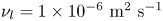 $\nu _{l}= 1\times 10^{-6}\ {\rm m}^2\ {\rm s}^{-1}$,
  $\sigma _{l} = 0.073\ {\rm N}\ {\rm m}^{-1}$; and an example of galvanizing conditions with zinc (Galvanization), with
  $\rho _{l}=6500\ {\rm kg}\ {\rm m}^{-3}$,
  $\nu _{l}= 4.5\times 10^{-7}\ {\rm m}^2\ {\rm s}^{-1}$,
  $\sigma _{l} = 0.78\ {\rm N}\ {\rm m}^{-1}$.

Table 2 also shows that the newly investigated conditions with water are significantly different from previous test cases and much closer to galvanizing conditions. In particular, the similarity in terms of  $[h]/Z$,
  $h_f/[h]$,
  ${Ca}$,
  $\varPi _g$ and
  $\mathcal {T}_g$ is remarkable, suggesting that the overall wiping mechanism reaches a good degree of similitude. On the other hand, significant differences remain in terms of the Reynolds number in both the liquid and the jet and the Kapitza number, suggesting that the impact of turbulence phenomena in both flows and the interface damping due to surface tension might be underestimated.
3. Methodology
This section describes the numerical configuration of the CFD simulations (§ 3.1), the modal analysis techniques applied to capture the instability mechanism (§ 3.2) and the theoretical foundations of the liquid-film models for jet wiping (§ 3.3).
3.1. Three-dimensional VOF LES simulations
The selected test cases are simulated using the open-source CFD software OpenFOAM (Weller et al. Reference Weller, Tabor, Jasak and Fureby1998), and the numerical model combines the algebraic VOF formulation of the interFoam solver with the Smagorinski LES model for the turbulence treatment of the gas jet flow. Barreiro-Villaverde et al. (Reference Barreiro-Villaverde, Gosset and Mendez2021) previously validated this approach with experiments, both in terms of stationary (mean final coating thickness) and non-stationary flow features (coherent structures and frequency content of both gas jet and liquid film). The LES technique involves the low-pass filtering of the equations with a Gaussian spatial filter  $\boldsymbol {G}_\varDelta (\boldsymbol {x})$ such that
  $\bar {\phi } = \boldsymbol {G}_\varDelta (\boldsymbol {x}) \circledast \phi$ where
  $\phi$ denotes the flow variables, the
  $\circledast$ the convolution operator and the overbar refers to the filtered flow variables. Therefore, the incompressible Navier–Stokes system reads
 $$\begin{gather} \boldsymbol{\nabla}\boldsymbol{\cdot}\bar{{\boldsymbol{u}}} = 0 , \end{gather}$$
 $$\begin{gather}\frac{\partial \left( \bar{\rho} \bar{\boldsymbol{u}}\right) }{\partial t} + \left( \bar{\rho} \bar{\boldsymbol{u}} \boldsymbol{\cdot}\boldsymbol{\nabla}\right) \bar{\boldsymbol{u}} ={-} \boldsymbol{\nabla} \bar{p} + \bar{\rho} \boldsymbol{g} + \boldsymbol{\nabla} \boldsymbol{\cdot} [ 2\bar{\mu} \bar{\boldsymbol{\mathsf{S}}}] + \bar{F}_\sigma - \boldsymbol{\nabla} \boldsymbol{\cdot} \boldsymbol{\tau} , \end{gather}$$
where  ${\boldsymbol {u}}=(u,v,w)$ is the velocity,
  $p$ the pressure,
  $\boldsymbol {g}$ is the gravitational acceleration,
  $\mu$ the dynamic viscosity,
  $\boldsymbol{\mathsf{S}}=(\boldsymbol {\nabla }{\boldsymbol {u}} + \nabla ^{T}{\boldsymbol {u}})/2$ the strain rate tensor,
  $F_\sigma$ the term accounting for the Laplace pressure computed using the continuum surface force model of Brackbill, Kothe & Zemach (Reference Brackbill, Kothe and Zemach1992) and
  $\boldsymbol {\tau }$ the subgrid stress term. This last term accounts for the turbulent stresses at scales smaller than the spatial filter, which in the Smagorinski model are computed as
 \begin{equation} {\tau_{u} ={-}2 \mu_t \bar{\boldsymbol{\mathsf{S}}} ,} \quad {\mu_t = \rho (C_s \Delta x_{cell})^2 |\bar{\boldsymbol{\mathsf{S}}}| .} \end{equation}
 The system is completed with the algebraic VOF implementation in interFoam (Deshpande, Anumolu & Trujillo Reference Deshpande, Anumolu and Trujillo2012), which solves an additional transport equation for the liquid volume fraction  $\alpha$,
 \begin{equation} \frac{\partial \bar{\alpha}}{\partial t} + \boldsymbol{\nabla}\boldsymbol{\cdot}(\bar{{\boldsymbol{u}}} \bar{\alpha}) + \boldsymbol{\nabla}\boldsymbol{\cdot} \left(\bar{{\boldsymbol{u}}}_r \bar{\alpha} (1-\bar{\alpha}) \right) = 0 , \end{equation}
where the last term introduces an artificial velocity  $\bar {{\boldsymbol {u}}}_r$ at the interface to mitigate its smearing. It is important to note that we neglect the extra subgrid terms due to unresolved surface tension terms and surface deformation due to the phase-averaging of VOF and the low-pass filtering of the LES (see Lakehal (Reference Lakehal2018) for more details). The large-eddy interface simulation models aim at providing closure models for the interfacial subgrid terms, although these are very case dependent and their implementation is only justified in cases where the subgrid scales are relevant to the flow, such as in jet atomization.
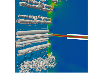
The domain and the mesh are shown in figure 2. The domain includes the coating bath from which the flat substrate is withdrawn, and a portion of the slot nozzle from which the gas jet is released. It spans 50 mm above and below the jet axis in the streamwise direction ( $x$), 20 mm in addition to the standoff distance
  $Z$ in the cross-stream direction (
 $y$) and 20 mm in the spanwise direction (
 $z$). The boundary conditions are indicated in figure 2, and the gas jet is established through an inlet condition with prescribed stagnation pressure
  $\Delta P_N$. Turbulence is promoted by introducing white noise perturbation with an amplitude of 5 % of the jet inlet velocity. The lateral patches (not shown) are set to cyclic.
Numerical domain, boundary conditions and mesh discretization.

The discretization is particularly challenging because of the multiscale nature of the problem, requiring a resolution of the order of the micrometre in different regions of the domain and along different directions. Since a complete mesh sensitivity analysis was out of the reach of our computational resources, the mesh design was based on (i) scaling considerations, (ii) the successful experimental validation of the simulations in Barreiro-Villaverde et al. (Reference Barreiro-Villaverde, Gosset and Mendez2021) and (iii) a set of preliminary tests. More specifically, the meshing near the moving strip was carried out keeping the same aspect ratio and the same dimensionless resolution across the liquid film as in Barreiro-Villaverde et al. (Reference Barreiro-Villaverde, Gosset and Mendez2021).
These considerations lead to a cell size in the region of gas–liquid interaction ( $-Z< x< Z$) of
  $\varDelta _x=50\ \mathrm {\mu }{\rm m}$ and
  $\varDelta _y=2\ \mathrm {\mu }{\rm m}$ across the film thickness. This provides 10 to 15 mesh points within the liquid film and 100 to 200 mesh points within one wavelength of the leading mode in the streamwise direction. This wavelength was first estimated from the results in Barreiro-Villaverde et al. (Reference Barreiro-Villaverde, Gosset and Mendez2021), scaled according to the reference quantities in table 1, and then confirmed a posteriori by the modal decomposition of the results. In dimensionless coordinates, this is much finer than the mesh in Aniszewski et al. (Reference Aniszewski2021) which allowed for a maximum of four points within the liquid film in the 2-D simulation and less than one mesh point within the film in the 3-D simulations.
On the gas side, the mesh was designed using the Taylor microscale in the nozzle as a reference. This characteristic length was estimated as  $\lambda _T = (10 k \nu _g / \epsilon )^{0.5}$, with
  $k$ the turbulent kinetic energy and
  $\epsilon$ the turbulent dissipation, computed using the empirical procedure in Rodriguez (Reference Rodriguez2019),
 \begin{equation} {k=\frac{3}{2} (U_J I )^2, \qquad \epsilon =C_{\mu} \frac{k^{2/3}}{ \ell },} \end{equation}
with  $U_J$ the mean velocity of the jet,
  $I$ the turbulence intensity estimated as
  ${I=0.144 Re_j^{-0.146}}$,
  $C_\mu = 0.09$ and
  $\ell =0.07 D_h$ the integral length scale based on the hydraulic diameter
  $D_h \approx 2d$. This estimation leads to
  $\lambda _T\approx 230\ \mathrm {\mu }{\rm m}$ for case 3 and
  $\lambda _T\approx 220\ \mathrm {\mu }{\rm m}$ for case 4. The mesh resolution in the streamwise direction was thus set to
  $\varDelta _y = 100\ \mathrm {\mu }{\rm m}$, as a good compromise between resolution and cost and to keep
  $\varDelta _y/\lambda _T<1/2$ in all simulations. In absolute terms, the resolution is comparable to the one in Aniszewski et al. (Reference Aniszewski2021). However, these authors consider a flow at much higher velocity (
 ${{Re}_J\approx 14\,300}$), leading to
  $\varDelta _y/\lambda _T>1$. In the cross-streamwise direction, the resolution was set to
  $\varDelta _x = 10\ \mathrm {\mu }{\rm m}$, leading to
  $y^+<5$ at the nozzle's wall for all cases. Finally, the spanwise resolution was set to
  $\varDelta _z=250\ \mathrm {\mu }{\rm m}$, keeping a similar aspect ratio in the spanwise direction as in Barreiro-Villaverde et al. (Reference Barreiro-Villaverde, Gosset and Mendez2021) and expecting a predominantly 2-D dynamics in the flow as in the previous works. The final mesh count reaches
  $14\times 10^6$ hexahedral cells.
The mesh quality was also assessed a posteriori using the LES index proposed in Celik, Cehreli & Yavuz (Reference Celik, Cehreli and Yavuz2005),
 \begin{equation} L_e = \frac{1}{1+\alpha_{\nu} \left( \dfrac{\nu_t}{\nu} \right)^n} , \end{equation}
with  $\alpha _{\nu } = 0.05$ and
  $n=0.53$ from correlations, and
  $\nu _t=\mu _t/\rho _g$ the turbulent viscosity from the simulations, computed from (3.2a,b). The LES index is above
  $80\,\%$ in the wiping region in all cases, following the recommendations in Pope (Reference Pope2000).
The simulations are initialized as in Barreiro-Villaverde et al. (Reference Barreiro-Villaverde, Gosset and Mendez2021) following two steps. The first phase begins with a uniform thickness distribution on the strip with  $\hat {h}=1$ and ends with the establishment of a drag-out flow in the absence of the jet. This requires approximately
  $100$ ms of physical time. The second phase introduces the jet flow and ends after the wiping meniscus is established. This requires approximately 100 ms to simulate the initial transient, after which 350 ms of physical time is computed. The time step is
  $10^{-7}$ s to keep the Courant–Friedrichs–Lewy number below 0.9, and a total of
  $n_t=3500$ instantaneous flow fields are exported with a sampling rate of 10 kHz. The computation requires approximately 1000 hr running in parallel on 512 Intel E5–2680v3 CPUs from the Centro de Supercomputacion de Galicia (CESGA) for one test case with water (case 3), and a total of
  $5\times 10^6$ CPU hours for the four test cases.
3.2. Multiscale proper orthogonal decomposition
The results are processed using the multiscale proper orthogonal decomposition (mPOD) (Mendez, Balabane & Buchlin Reference Mendez, Balabane and Buchlin2019a; Mendez Reference Mendez2023) and its extension, as in Barreiro-Villaverde et al. (Reference Barreiro-Villaverde, Gosset and Mendez2021). This technique decomposes the data  $\boldsymbol{\mathsf{D}}(\boldsymbol {x},t)$ as a linear combination of modes such that
 \begin{equation} {\boldsymbol{\mathsf{D}}(\boldsymbol{x},t)=\sum^{R}_{r=1} \sigma_r \boldsymbol{\phi}_r(\boldsymbol{x}) \boldsymbol{\psi}_r(t),} \end{equation}
where  $\sigma _r$ is the mode amplitude,
  $\boldsymbol{\phi} _r(\boldsymbol {x})$ is the mode spatial distribution and
  $\boldsymbol{\psi}_r (t)$ its temporal evolution. The structures
  $\boldsymbol{\phi} _r$ and
  $\boldsymbol{\psi} _r$ form, respectively, a basis for spatial distribution and temporal evolution of the data, while
  $\sigma _r$ indicates the energetic weight of each structure in the dataset. The mPOD is a data-driven decomposition that bridges the gap between the energy-based proper orthogonal decomposition (POD) (Sirovich Reference Sirovich1991; Holmes, Lumley & Berkooz Reference Holmes, Lumley and Berkooz1996) and frequency-based dynamic mode decomposition (Rowley et al. Reference Rowley, Mezić, Bagheri, Schlatter and Henningson2009; Schmid Reference Schmid2010) methods. In particular, the mPOD modes are optimal modes for a prescribed frequency partition and have a band-limited frequency content.
In a first step, we decompose the normalized film thickness, defined as  $\check {h} (x,z,t) = ({h(x,z,t) - \bar {h}(x,z)})/{\sigma _h (x,z)}$ with
  $\bar {h} (x,z)$ the average thickness and
  $\sigma _h (x,z)$ the thickness standard deviation (Barreiro-Villaverde et al. Reference Barreiro-Villaverde, Gosset and Mendez2021). This normalization allows the decomposition to equalize the importance of waves upstream and downstream of the wiping region despite the largely different thickness. Since we are interested in the most dominant travelling wave patterns, described by two sinusoidals in quadrature (phase-shifted by
  ${\rm \pi} /2$) both in time and space, we only retain the pair of modes
  $\mathcal {M}$ with the largest and equal amplitudes (
 $\sigma _{\mathcal {M}}$), having spatial (
 $\boldsymbol{\phi}_{\mathcal {M}}$) and temporal structures (
 $\boldsymbol{\psi}_{\mathcal {M}}$) in quadrature.
In a second step, we extract the most correlated coherent structures in the gas jet by projecting variables linked to the jet flow (e.g. velocity field, pressure or shear stress distribution at the wall) onto the dynamics of the leading wave patterns. Therefore, denoting as  $\boldsymbol{\mathsf{D}}_g (\boldsymbol {x},t)$ the general jet flow variable and as
  $\boldsymbol{\psi} _{\mathcal {M}}(t)$ the temporal structures of the leading wave pattern in the film thickness, the spatial distribution of the most correlated pattern is defined as
 \begin{equation} {\boldsymbol{\phi}_g(\boldsymbol{x})
= \frac{\langle \boldsymbol{\mathsf{D}}_g (\boldsymbol{x},t),
\boldsymbol{\psi}_{\mathcal{M}} (t)\rangle_t}{\sigma^2_{\mathcal{E}}}\quad \mbox{with}\
\sigma_{\mathcal{E}}=|| \langle \boldsymbol{\mathsf{D}}_g
(\boldsymbol{x},t), \boldsymbol{\psi}_{\mathcal{M}} (t)\rangle_t||_s} ,
\end{equation}
\begin{equation} {\boldsymbol{\phi}_g(\boldsymbol{x})
= \frac{\langle \boldsymbol{\mathsf{D}}_g (\boldsymbol{x},t),
\boldsymbol{\psi}_{\mathcal{M}} (t)\rangle_t}{\sigma^2_{\mathcal{E}}}\quad \mbox{with}\
\sigma_{\mathcal{E}}=|| \langle \boldsymbol{\mathsf{D}}_g
(\boldsymbol{x},t), \boldsymbol{\psi}_{\mathcal{M}} (t)\rangle_t||_s} ,
\end{equation}
where  $\langle \boldsymbol{a}(t),\boldsymbol{b}(t)\rangle _t=1/T\int ^T_0 \boldsymbol{a}(t) \boldsymbol{b}(t)\,{\rm d}t$ is the inner product in time, and
  $||\boldsymbol{a}(\boldsymbol {x})||^2_s=1/|\varOmega |\int _{\varOmega } \boldsymbol{a}^2(\boldsymbol {x})$ is the
  $L_2$ norm in space, with
  $\varOmega$ the simulation volume and
  $|\varOmega |$ its measure. The denominator in (3.7) has the scope of having
  $||\boldsymbol {\phi} _{g}(\boldsymbol {x})||_s=1$. The projection of a dataset (e.g. velocity field) onto the leading structures of another dataset (e.g. film height evolution) was first proposed by Borée (Reference Borée2003) for the POD and referred to as ‘extended’ POD. Barreiro-Villaverde et al. (Reference Barreiro-Villaverde, Gosset and Mendez2021) use the same idea for the ‘extended’ mPOD (emPOD).
3.3. One-dimensional analytical model for jet wiping
Analytical models for jet wiping were initially derived to predict the final thickness profiles as a function of the process parameters (Thornton & Graff Reference Thornton and Graff1976; Tuck Reference Tuck1983; Ellen & Tu Reference Ellen and Tu1984; Yoneda Reference Yoneda1993; Buchlin Reference Buchlin1997), and then extended to quasisteady formulations by Hocking et al. (Reference Hocking, Sweatman, Fitt and Breward2011) and more advanced integral formulations in Mendez et al. (Reference Mendez, Gosset, Scheid, Balabane and Buchlin2021).
Early validations of these models were limited to the final film thickness. A more extensive validation of the whole average thickness distribution for steady state models was presented by Lacanette et al. (Reference Lacanette, Gosset, Vincent, Buchlin and Arquis2006), while Barreiro-Villaverde et al. (Reference Barreiro-Villaverde, Gosset and Mendez2021) explored the validity of integral models in dynamic conditions. However, both Lacanette et al. (Reference Lacanette, Gosset, Vincent, Buchlin and Arquis2006) and Barreiro-Villaverde et al. (Reference Barreiro-Villaverde, Gosset and Mendez2021) considered the case of highly viscous fluids. In this work, we extend the validation to the wiping of water, both in time averaged and time-dependent conditions.
Thin film models build upon the 2-D incompressible Navier–Stokes equations for the liquid film, simplified using the longwave approximation. The later assumes that the characteristic length scale in the streamwise direction ( $x$) is much larger than in the cross-stream (
 $y$), i.e. the perturbation wavelength
  $\lambda$ is large compared with the liquid film thickness
  $h$. The separation of scales is provided by the film parameter
  $\varepsilon = [h]/[x]=Ca^{1/3}$ introduced in § 2. Neglecting terms of order
  $>O(\varepsilon )$, integrating the equations along the cross-stream direction using the Leibniz rule yields the following system of PDEs constituting the IBL model (Mendez et al. Reference Mendez, Gosset, Scheid, Balabane and Buchlin2021):
 $$\begin{gather} {\partial_{\hat{t}} \hat{h}+\partial_{\hat{x}} \hat{q}=0, } \end{gather}$$
 $$\begin{gather}{\varepsilon \,Re \left( \partial_{\hat{t}} \hat{q}+\partial_{\hat{x}} \mathcal{F} \right)=\hat{h} \left( 1-\partial_{\hat{x}} \hat{p}_{g}+\partial_{\hat{x} \hat{x} \hat{x}} \hat{h}\right) + \hat{\tau}_{g} - \hat{\tau}_{w} ,} \end{gather}$$
where  ${Re}=[u][x]/\nu _l = \sqrt {U_p^3 /g \nu _l}$ is the Reynolds number,
  $\hat {q}$ is the volumetric flow rate per unit width,
  $\partial _{\hat {x}} \hat {p}_g$ and
  $\hat {\tau }_g$ are the pressure gradient and shear stress distribution at the interface produced by the impinging jet,
  $\mathcal {F} = \int _{0}^{\hat {h}} \hat {u}^{2} \,{\rm d} \hat {y}$ is the integral advection term and
  $\hat {\tau }_{w} = \partial _{\hat {y}} \hat {u}|_{\hat {y}=0}$ is the shear stress at the wall. These last two terms require some assumptions on the streamwise velocity profile. The simplest IBL model assumes a parabolic, self-similar profile. Using the boundary conditions and the definition of the flow rate per unit width, it can be written as
 \begin{equation} \hat{u}= \left(\frac{3 \hat{q}}{\hat{h}}-\frac{3}{2} \hat{h}+3 \right) \left[\left(\frac{\hat{y}}{\hat{h}}\right)-\frac{1}{2}\left(\frac{\hat{y}}{\hat{h}}\right)^{2}\right]+\hat{\tau}_{g} \hat{y}-1, \end{equation}
leading to the following closure for (3.8):
 \begin{equation} {\mathcal{F}=\frac{\hat{h}^{3} \hat{\tau}_{g}^{2}}{120}+\frac{\hat{h} \hat{q} \hat{\tau}_{g}}{20}+\frac{\hat{h}^{2} \hat{\tau}_{g}}{20}+\frac{6 \hat{q}^{2}}{5 \hat{h}}+\frac{2 \hat{q}}{5}+\frac{\hat{h}}{5}} \quad{\text{and}}\quad \tau_w ={-}\frac{3\hat{q}}{\hat{h}^2} - \frac{3}{\hat{h}}. \end{equation}
 It is worth noticing that the boundary condition is  $\hat {u}(0)=-1$: keeping the classic convention in the literature of falling liquid films, the streamwise axis points downwards (same direction as gravity), contrary to the axes in the numerical simulations presented in this work.
The integral model in Hocking et al. (Reference Hocking, Sweatman, Fitt and Breward2011) can be obtained by neglecting inertia, hence  $\mathcal {F}=0$. In a further simplification, the steady state models in Tu & Ellen (Reference Tu and Ellen1986) and Buchlin (Reference Buchlin1997) can be reached by also removing the surface tension and time dependent terms. In these conditions, since
  $\partial _{\hat {x}} \hat {q} = 0$, the system of equations in (3.8) reduces to a cubic equation in terms of film thickness
  $\hat {h}$, with
  $\hat {q}$ left as a free parameter,
 \begin{equation} {\left( \partial_{\hat{x}} \hat{p} + 1 \right) \hat{h}^3 - \tfrac{3}{2}\hat{\tau}_g \hat{h}^2 - 3\hat{h} + 2 \hat{q} = 0}. \end{equation}
 This is known as the zero-order model. At each position  $x$, the cubic equation (3.11) admits two positive solutions. The blending between these allows recovering the full interface distribution. Independently from their respective degree of approximation, all these models require as inputs the distributions of pressure gradient and shear stress at the film interface (see Gosset (Reference Gosset2007) for a review). This is why to assess these models in the best possible conditions, we extract the stress distributions from the numerical results.
4. Results
The results of the two-phase simulations are first compared with thin film models in terms of average thickness and velocity profiles in § 4.1. Section 4.2 analyses the wave patterns on the liquid film, while § 4.3 focuses on the gas flow structures that are most correlated with the leading wave patterns. Finally, § 4.4 discusses the mechanism of interaction between the two phases. In all sections, the new results on cases 3 and 4 are analysed along with the ones previously obtained for cases 1 and 2. The spatiotemporal distribution of thickness  $h(x,z,t)$ and streamwise pressure gradient
  $\partial _x p(x,z,t)$ of cases 1 and 3 are openly available at http://doi.org/10.17605/OSF.IO/QAGBZ.
4.1. Cross-assessment of CFD and liquid-film models
As explained previously, the distributions of pressure gradient and shear stress at the interface are required to assess the thin film models in (3.3). These were retrieved from the postprocessing of the numerical results.
Starting from the averaged predictions, figure 3(a) shows the time-averaged distribution of pressure at the interface in the middle plane, i.e.  $z=L_z/2$, for case 3. A Gaussian distribution
  $\hat {p}_g(x)=\hat {p}_M\exp (-\hat {x}^2/\gamma _p)$ with
  $\hat {p}_M=43.5$ and
  $\gamma _p = 0.992$ appears appropriate. Figure 3(b) shows the link between the time averaged pressure gradient and the time averaged shear stress at the interface. Within the range
  $\hat {x}\in [-1,1]$, a reasonable correlation is provided by the linear trend
  $\tau _g(x)\approx -0.07 \partial _{\hat {x}}\hat {p}(x)+0.5\,\mbox {sign}(x)$, with
  $\mbox {sign}(x)=1$ if
  $x>0$,
  $\mbox {sign}(x)=-1$ if
  $x<0$ and
  $\mbox {sign}(0)=0$. The same approach was used for case 4.
Time-averaged dimensionless pressure distribution at the interface and the result of exponential fitting (a), and correlation between the pressure gradient distribution and the shear stress distribution at the interface (b). In both plots, the blue continuous line represents the CFD data, while the dashed red line represents the Gaussian and the linear fitting, respectively.
Introducing these distributions in the models (3.8) and (3.11) yields the results in figure 4. Figure 4(a) compares the results in terms of mean thickness profile for the CFD (orange solid line), the full IBL model in steady conditions (red dashed line) and the zero-order model (blue dotted line). The figure is complemented with a close-up above the wiping region and shaded areas to show the envelope of film thickness distributions. These were filtered using the emPOD to focus only on the leading travelling patterns. The model predictions were obtained using the pressure gradient and the shear stress distributions at the interface obtained by fitting an exponential curve on the pressure distribution and a linear fit between this and the shear stress. These are compared with the envelope values after filtering these quantities with the emPOD in figures 4(b) and 4(c), respectively.
Comparison between the CFD time averaged thickness profiles at  $z=L_z/2$ and the theoretical predictions using the zero-order and IBL model (a), together with the envelopes of the pressure gradient
  $\partial _x p$ (b) and shear stress
  $\tau _x$ (c). The solid lines in figures 4(b) and 4(c) represent the inputs of the theoretical models and have been obtained via Gaussian regression.

The overall agreement between the thin film models and the CFD is satisfactory in terms of average film thickness, especially considering the simplifying assumptions underpinning the models and the uncertainty on the wiping actuators. The IBL model provides an excellent prediction of the final film thickness and a satisfactory prediction of the meniscus shape. The discrepancy between the IBL and the zero-order model suggests that the surface tension and the advection term  $\mathcal {F}$, both neglected in the latter, are important. The large fluctuations of both the film thickness and wiping actuators illustrate the importance of the flow unsteadiness, analysed in detail in §§ 4.3 and 4.4.
Moving now to the dynamic conditions, the main interest is to analyse the validity of the self-similar parabolic profile underpinning the IBL model. This was shown to be surprisingly valid for cases 1 and 2 in Barreiro-Villaverde et al. (Reference Barreiro-Villaverde, Gosset and Mendez2021), despite the value of the film parameter ( $\varepsilon =[h]/[x]=0.93$), certainly too close to unity to justify the longwave approximation. Moreover, these cases are characterized by
  ${Re}\approx 7.4$, leading to a reduced Reynolds
  $\delta \approx \varepsilon \,{Re}= 6.8$ which is also outside the theoretical limit
  $\delta \sim O(1)$ above which the integral boundary layer approximation is in principle valid, as detailed in Kalliadasis et al. (Reference Kalliadasis, Ruyer-Quil, Scheid and Velarde2012). Cases 3 and 4 are characterized by a lower
  $\varepsilon =0.24$ but a much higher
  ${Re}\approx 320$, leading to
  $\delta \approx 77$. Figure 5 shows for case 1 (figure 5a) and case 3 (figure 5b), a contour plot of the streamwise velocity component in the
  $z$-midplane (
 $u(x,y,z=L_z/2)$) on the left-hand, with the horizontal red lines indicating the location from which the velocity profiles are extracted and plotted on the right-hand. These plots compare the CFD data (dashed blue) with the self-similar profile in (3.9). All variables are scaled by the reference quantities in table 1.
Contour map of the streamwise velocity with streamlines at the  $z$-midplane. The data are shown both in dimensional (left-hand side) and dimensionless axes (right-hand side). The horizontal red lines in the contours indicate the locations of the velocity profiles on the right-hand side. The continuous lines show the profile obtained with the simulation, and the dashed lines the self-similar profile in (3.9). (a) Case 1; (b) case 3.

The comparison of five profiles at different positions in the streamwise direction shows that the velocity profile remains close to parabolic, even at the much higher Reynolds number in case 3. This is true in all the domain for case 1 and only in absence of 3-D effects in case 3. For the illustrated snapshots, the validity of the parabolic assumption is particularly striking in the profile at  $x \approx -4$ mm (
 $\hat {x}<-2.2$) for case 1 and the profile at
  $x \approx -1.8$ mm (
 $\hat {x}=-1.3$) for case 3. Both are characterized by a large interface curvature and shear stress (see also figure 4c). Within
  $\hat {x}\in [-1,1]$, the dynamics of the flow field within the liquid film is quite similar, while differences become more pronounced as the waves in the run-back flow develop. At
  $x<-2$ mm (
 $\hat {x}<-1.7)$), the flow becomes 3-D for case 3 (as further illustrated in the following) and vortices appear between the crests of two successive waves. Therefore, while the parabolic assumption is appropriate in a large portion of the domain for case 1, its validity is confined to
  $\hat {x}>-1.5$ for case 3. Nevertheless, as discussed in the following sections, this is the area where most of the interaction between the gas jet and the liquid film takes place. Finally, we assess the validity of the key ingredient of the boundary layer approximation, allowing for neglecting the convective/inertial effect in the cross-stream direction in the film, and assuming zero cross-stream pressure gradient. To this end, figure 6 shows the pressure profiles at the interface
  $\hat {p}_i=\hat {p}(\hat {y}=\hat {h})$ and at the wall
  $\hat {p}_w = \hat {p}(\hat {y}=0)$ (figure 6a), the instantaneous film thickness distribution (figure 6b) and the standard deviation of the differential pressure across the film
  $\sigma _{\Delta \hat {p}}$, where
  $\Delta \hat {p} = \hat {p}_i - \hat {p}_w$ (figure 6c). The pressure at the wall and at the interface are identical in the final film, while some variations are visible in the run-back flow, where the flow is forced to reverse direction due to the wiping effect of the jet. This, together with the larger thickness and local Reynolds number make the cross-stream inertia more important and challenge the validity of the boundary layer approximation.
Dimensionless pressure profiles at the wall  $\hat {p}_w = \hat {p}(\hat {y}=0)$ and at the interface
  $\hat {p}_i = \hat {p}(\hat {y}=\hat {h})$ (a) and thickness (b) for a given time step, together with the standard deviation
  $\sigma _{\Delta \hat {p}}$ of the dimensionless pressure difference across the film
  $\Delta \hat {p} = \hat {p}_w - \hat {p}_i$ (c).

4.2. Wave patterns on the liquid film
Figure 7 illustrates the dynamics of the liquid film upstream of the wiping region ( $x<0$) in case 1 (figure 7a) and 3 (figure 7b). In each plot, an instantaneous film thickness distribution is shown, with the liquid going upwards in red (
 $u>0$) and the liquid going downwards in green (
 $u<0$). In case 1, the liquid film is clearly 2-D and features large waves originating approximately
  $2.5$ mm below the jet axis at a frequency of approximately
  $20$ Hz, corresponding to
  $\hat {f}=f{[t]} \approx 0.11$ in the scaling from table 1. These falling waves have a wavelength of the order of
  $\lambda \approx 12$ mm and evolve over an average film thickness of the order of
  $h_r\approx 2h_0=3$ mm. The local Reynolds number in this region, defined as
  ${Re}_r=h_r \Delta U/\nu$, with
  $\Delta U = \max (U_p - u|_{y=h}) \approx 2U_p$ is of the order of
  $Re_r\approx 18$. The flow is fairly laminar, and the 2-D nature of the falling waves is in line with what happens at the onset of interface instability in falling liquid films. Case 3 is clearly in a different wiping regime, especially from the liquid perspective as indicated in table 2. The frequency of wave formation (
 $f \approx 100\unicode{x2013}150$ Hz) in the introduced scaling is
  $\hat {f} \approx 0.15\unicode{x2013}0.2$, a value notably close to the one in case 1. The reasonable matching of the dimensionless frequencies in the two wiping regimes reinforces the choice of the reference quantities used for scaling, and justifies the dimensionless representation adopted in subsequent comparisons. The effect of increasing the film Reynolds number in case 3 (
 $Re_r\approx 800$) is clearly visible on the wave patterns on the run-back flow. The waves emerge 2-D – similar to case 1 – at approximately
  $0.5$ mm below the jet axis, but they rapidly undergo a transition towards a 3-D pattern, reminiscent of what occurs in falling liquid films (see Demekhin et al. Reference Demekhin, Kalaidin, Kalliadasis and Vlaskin2007).
Snapshots of the film thickness dynamics in cases (a) 1 and (b) 3. The liquid is coloured in red where  $u>0$ and in green where
  $u<0$. A supplementary movie of the 3-D reconstruction of the liquid film is also provided for both cases and is available at https://doi.org/10.1017/jfm.2024.553.

Moving to the multiscale modal analysis of the liquid film thickness, the convergence of the decomposition is illustrated in figure 8 as a function of the normalized energy content of the modes  $(\sigma _r / \sigma _1)^2$. The modes denoted with a full marker correspond to the ones that are selected as dominant wave patterns following the criterion defined in § 3.2. For each test case, figure 9 shows a snapshot of the normalized liquid film thickness (figure 8a i,b i,c i,d i), its reconstruction using the leading mPOD modes linked to the dominant travelling wave pattern (figure 8a ii,b ii,c ii,d ii) and the spectra of the associated temporal structures (figure 8a iii,b iii,c iii,d iii). The wiping conditions are recalled in the caption. The spectra computed from the temporal structure of the leading modes are represented as a function of both the dimensional
  $f$ and dimensionless
  $\hat {f}$ wave frequencies. Note that the stream and spanwise coordinates are shown in dimensionless form to facilitate the comparison between cases, since the dimensional wavelengths (and frequencies) are very different, as illustrated previously with figure 7.
Convergence of the mPOD decomposition for all cases. The dominant modes in figure 9 are denoted with a full marker.

Comparison between snapshots of the normalized film thickness  $\check {h}(\hat {x},\hat {z})$ (i) with the leading wave patterns detected via mPOD (ii). The spectra of the temporal structure of these modes are shown in (iii) as a function of the dimensional
  $f$ and dimensionless
  $\hat {f}$ wave frequencies. (a) Case 1 (DG),
  $\hat {Z}=14.2$,
  ${\varPi _g =0.16}$,
  $\mathcal {T}_g = 0.24$; (b) case 2 (DG),
  $\hat {Z}=14.2$,
  $\varPi _g =0.33$,
  $\mathcal {T}_g = 0.41$; (c) case 3 (W),
  $\hat {Z}=10$,
  $\varPi _g =1.02$,
  ${\mathcal {T}_g = 2.23}$; (d) case 4 (W),
  $\hat {Z}=10$,
  $\varPi _g =1.53$,
  $\mathcal {T}_g = 3.02$.

The slow convergence of the decomposition illustrates the complexity of the flow, as it appears from the normalized film thickness  $\check {h}$ distributions on the left-hand side. Even if the original (unfiltered) fields depict different dynamics, the mPOD analysis detects similar dominant wave patterns in both the run-back flow and final film. In all the cases, the leading wave pattern is remarkably 2-D, despite the vastly different wiping conditions, and regardless of the 3-D patterns arising upstream of the wiping region with water.
This is linked to the fact that the energy of the modes is more biased towards the final film in the cases with water because the 2-D dominant pattern, although present, is less important in the run-back flow. The energy in the run-back flow is distributed within more modes, featuring 3-D waves at slightly different wavelengths and frequencies. The dominant wavelength upstream and downstream of the wiping differs because of the different advection velocities in the two regions, but like in the run-back film, the range of dimensionless frequency is surprisingly similar (0.1–0.3). In line with the experimental findings with low  $\textit {Ka}$ liquids in Gosset et al. (Reference Gosset, Mendez and Buchlin2019), the frequency tends to increase with the wiping strength, and the gas jet Strouhal number
  ${St}=f Z / U_j$ based on the dominant frequency of the waves, is in the range (0.01–0.04), well below the typical values in free-jet instability and hydrodynamic feedback mechanisms (Mendez, Scelzo & Buchlin Reference Mendez, Scelzo and Buchlin2018). These results highlight the important coupling between the gas jet and the liquid. The following section analyses the gas jet structures linked to those dominant wave patterns.
4.3. Gas jet structures correlated with the leading waves in the liquid film
The dynamics of the gas jet and its connection to the dominant wave patterns has seldom been explored in the literature, due to the challenges in the experimental characterization and the computational cost of high-fidelity simulations. Figure 10 depicts the complexity of the gas jet dynamics for case 1 (figure 10a) and 3 (figure 10b). For both cases, the velocity contours at the  $z$-midplane are shown on the left-hand side while a 2-D view of the film in a plane parallel to the moving substrate is shown on the right-hand side. The gas jet structures, extracted using the
  $Q$-criterion, are shown in grey while the liquid film interface is shown in represented in blue shades.
Flow visualization of case (a) 1 and (b) 3. The gas jet vortices extracted using the  $Q$-criterion (grey) are superimposed to the liquid film interface (blue) and a contour plot of the velocity magnitude in the (a)
  $x\unicode{x2013}y$ plane and (b)
  $x\unicode{x2013}z$ plane for each test case: (a) case 1 (DG); (b) case 3 (W).

The dynamics of the jet are comparable, as expected from the similarity of the jet Reynolds number  ${Re}_j$ (see table 2). At a short distance from the nozzle, 2-D vortices are generated in the shear layers, due to the velocity gradient between the jet core and the quiescent atmosphere. At impingement, these vortices produce a low-amplitude/high-frequency flapping of the jet tip. Then, the main flow splits into two ‘side jets’ that remain attached to the gas–liquid interface until the run-back waves become too steep and trigger flow detachment. Downstream of the wiping, the 2-D vortices are convected along with the side jets and in close interaction with the interface. Finally, these structures undergo transverse modulation and dissipate into smaller eddies. Upstream of the wiping, it is interesting to note that the 2-D–3-D transition seems to be enhanced by the presence of the waves on the run-back flow, especially in case 3 where the vortices become 3-D very close to the impact. Comparatively, they remain unaltered for longer distances on the final film, which suggests the gas–liquid interaction is negligible in this region. These flow visualizations confirm that the gas jet perturbation is essentially 2-D, and therefore, uncorrelated with the formation of 3-D waves on the liquid, as expected from the analysis in § 4.2. This was previously observed in Barreiro-Villaverde et al. (Reference Barreiro-Villaverde, Gosset and Mendez2021) for case 2 using correlation analysis, and is confirmed here for different wiping conditions.
We now focus on the spatial structures in the gas jet flow using the emPOD, to reveal the flow structures that are most correlated with the leading wave patterns on the liquid film (described in figure 9). Figure 11 shows two representative snapshots of the gas velocity field  $\boldsymbol {u}=(u,v)$ at the
  $z$-midplane and its projection for case 1 (figure 11a) and case 3 (figure 11b). Cases 2 and 4 lead to similar results and are thus omitted for brevity, but an animation of the film thickness evolution and gas jet flow for each test case is provided in the supplementary material. In each figure, the contour on the left-hand side is the mean centred flow field (i.e.
  $\boldsymbol {u}^\prime = \boldsymbol {u}(\boldsymbol {x}) - \bar {\boldsymbol {u}}$), and the one on the right-hand side is the projection of the flow field on the leading mPOD modes of the normalized film thickness.
Mean-centred  $u^\prime$ and emPOD projected fields for cases (a) 1 and (b) 3. The plots are scaled such that the horizontal axis ranges between
  $0< y/Z<1$, and the vertical axis between
  $-10< x/d<10$. A supplementary movie for each test case in table 2 is also provided. (a) Case 1 (DG); (b) case 3 (W).

While the original flow fields reveal the full spectrum of flow structures, the emPOD filtered fields retain only those that are temporally correlated with the main patterns on the liquid layer or, from a physical perspective, those that are mostly correlated to the gas–liquid coupling. For instance, the vortices in the shear layers (label ‘ $v_s$’) and their downstream evolution (label ‘
 $v_f$’) are not visible in the emPOD counterpart, confirming that these structures are not correlated with the main wave pattern. Their impact on the liquid film is limited to small-scale disturbances that are rapidly damped due to viscosity and capillarity (Barreiro-Villaverde et al. Reference Barreiro-Villaverde, Gosset, Lema and Mendez2023). Here, the leading structures consist of a larger vortex induced by the falling liquid waves (label ‘
 $v_r$’) and a rigid oscillation of the impinging jet (label ‘
 $d$’). In the case of low Kapitza liquids, this mechanism was extensively documented in Myrillas et al. (Reference Myrillas, Rambaud, Mataigne, Anderhuber, Gardin, Vincent and Buchlin2013), Mendez et al. (Reference Mendez, Gosset and Buchlin2019b) and Barreiro-Villaverde et al. (Reference Barreiro-Villaverde, Gosset and Mendez2021), where a hypothesis on their interaction with the liquid film dynamics was formulated. In particular, it was postulated that the jet oscillation was linked to the vortex–liquid film interaction. The current results with high
  $\textit {Ka}$ liquids show for the first time that this interaction is much weaker in these conditions because of the comparatively smaller thickness of the liquid film; yet, these structures ‘
 $v_r$’ and ‘
 $d$’ persist. Is it because the gas–liquid interaction is similar despite the different flow conditions? Which comes first, the waves in the liquid or the oscillations/deflections in the gas? Is it possible to extrapolate these results to industrial galvanization? These questions are addressed in § 4.4.
4.4. Dynamics of the gas–liquid instability
Previous sections focused on the relevant flow patterns in the liquid film and the gas jet; this section investigates their impact on the momentum transfer at the interface. For two snapshots separated by half-undulation period  $T$, figure 12 shows the emPOD filtered dimensionless pressure gradient
  $\partial _{\hat {x}} \hat {p} = \partial _x p [x]/[p]$ and dimensionless shear stress
  $\hat {\tau }_{\hat {x}} = \tau _x / [\tau ]$ for case 1 (figure 12a) and case 3 (figure 12b).
Spatiotemporal evolution of the pressure gradient  $\partial _{\hat {x}} \hat {p}$ and shear stress
  $\hat {\tau }_{\hat {x}}$ in case (a) 1 and case (b) 3 for two time steps separated by half an undulation cycle
  $T$. (a) Case 1 (DG); (b) case 3 (W).

In both cases, the distributions downstream of the wiping ( $\hat {x}>0$) remain more or less unaffected – as expected from the negligible activity shown in figure 11 at these locations. The unsteadiness of the wiping actuators is concentrated in the run-back flow, featuring pulsations and oscillations of the wiping point
  $x^*$ (
 $\partial _x p (x^*) = \max (\partial _x p)$) and the shear point
  $x_\tau$ (
 $\tau _x (x_{\tau }) = \max ({\rm abs}(\tau _x)$), due to the interaction between the lower side jet and the run-back waves.
The connection between the dynamics of the liquid film and wiping actuators is analysed by means of the spatiotemporal contour of the normalized film thickness  $\check {h}$ in figure 13 for case 1 (figure 13a) and 3 (figure 13b). This contour map is complemented with the temporal evolution of (i) the impingement point
  $x_p$ (
 $p (x_p) =$ max(
 $p$)) (dashed red line) and (ii) the wiping point
  $x^*$ (continuous white line). The streamwise coordinate is normalized with the jet opening
  $d$ and time axis is scaled as
  $\hat {t}= t / [t]$. The region delimited by these two points is referred to as wiping region, i.e. the region where most of the wiping work occurs. Here, the characteristic lines are gently curved because of the wave acceleration due to the strong gas–liquid interaction. These characteristic lines are continuous in case 1, while the waves occasionally reverse direction in case 3. This is probably due to the reduced effect of the jet flow outside the wiping region, combined with a temporary win of the viscous drag over gravity and inertia. In all cases, it appears that the amplitude of the jet oscillation (linked to the jet structure ‘
 $d$’) has a minor role compared with the large fluctuations experienced by the wiping point (linked to the jet structure ‘
 $v_r$’). These fluctuations are characterized by a ‘slow’ downward dynamic and a ‘fast’ upward dynamic, as if the mechanisms governing these two stages were completely different. The downward shift of the wiping point occurs at the scale of the wave advection time in the falling liquid waves, while the upward shift occurs at the scale of the gas jet advection time. It is noteworthy that the waves are propagated at approximately the substrate speed (
 ${\hat {u} \approx 1}$) in both the final film and run-back flow, regardless of the wiping strength (
 $\varPi _g$), film intrusiveness (
 $h_0 / Z$) and characteristic speed of the side jet (
 $U_{sj}$) – which can reach values up to
  $\hat {u}_{sj} = 20$ in our simulations. This observation is in agreement with Lunz & Howell (Reference Lunz and Howell2018), who investigated a falling liquid film subjected to external pressure perturbations, and showed that the maximum amplification occurs when the pressure disturbance moves at a speed comparable to the wave propagation.
Spatiotemporal contours of the normalized film thickness  $\check {h}$ for cases (a) 1 and (b) 3, complemented with the temporal evolution of the impingement point
  $x_p$ (dashed red line) and the wiping point
  $x^*$ (continuous white line), both defined in the text. (a) Case 1 (DG); (b) case 3 (W).

From this perspective, the strip velocity plays a dominant role, while the wiping strength and the jet velocity plays a secondary role in selecting the coupling frequency. Tracking the white lines in figure 13, it appears that the time scale of the coupling is associated with (i) the time required to produce a wave in the run back flow, (ii) the time required for this wave to exit the wiping region. Below this zone, the wiping point is no longer able to ‘stick’ onto the wave's back and so it recovers its upward position, where a new wave will be generated. This mechanism is consistent with experimental data and the qualitative description in Mendez et al. (Reference Mendez, Gosset and Buchlin2019b), and justifies why a purely liquid-based scaling in which  $[u]=U_p$ yields similar dimensionless frequencies in largely different wiping regimes.
Finally, to conclude on the similarity between the investigated conditions, we analyse the time response of the liquid film thickness to the unsteadiness of the wiping point for both cases 1 and 3. Figure 14 compares the evolution of the emPOD filtered film thickness and pressure gradient at the time averaged wiping point  $\bar {x}^*$. The latter is defined as the location at which the time-averaged pressure gradient is maximum, i.e.
  $\bar {x}^*$ (
 $\overline {\partial _x p})(\bar {x}^*)=\mbox {max}(\overline {\partial _x p})$. The similarity between the two plots suggests that a comparable coupling mechanism takes place in the two cases despite the large differences in
  $\textit {Ka}$, wiping conditions and intrusiveness of the film. Because the dimensionless frequencies of the waves remain within the same range, we may infer that the interaction is mostly driven by the liquid film. Considering that the dimensionless groups related to the liquid film dynamics are in fair similarity between water and zinc (table 2), these results suggest that the coupling dynamics observed in water might not differ significantly from the one occurring in galvanization. It is striking that the wavy defects observed on galvanized products have typical wavelengths in the range 10–15 mm, which corresponds to dimensionless frequencies of
  $\hat {f} = (0.11\unicode{x2013}0.165)$, totally in line with what is found here for largely different conditions.
Lissajous curves for the dimensionless pressure gradient  $\partial _{\hat {x}} \hat {p}$ and thickness
  $\hat {h}$ at the time averaged wiping point
  $\bar {x}_*$ for case (a) 1 and (b) 3. (a) Case 1 (DG); (b) case 3 (W).

5. Conclusions
We have numerically investigated the two-phase coupling instability taking place between an impinging gas jet and a liquid film dragged by an upward moving substrate. The two-phase simulations with a high Kapitza liquid allowed for characterizing the gas–liquid interaction in an unexplored wiping regime and much closer to the industrial conditions, especially from the liquid perspective.
The results show a strong gas–liquid interaction which produces undulations on the final film, both with low and high Kapitza liquids. The waves emerge 2-D in the impingement region, even when the run-back flow is 3-D. It suggests that the 2-D–3-D transition of the liquid waves is due to an intrinsic instability typical of a falling film at these Reynolds numbers, and not due to the gas jet, which is fundamentally 2-D. The correlation analysis in the gas jet reveals two flow structures acting at the time scale of the leading wave pattern: a symmetric oscillation around the jet axis (pattern ‘ $d$’), and a deflection of the lower side jet triggered by the periodic formation of waves (pattern ‘
 $v_r$’). It is shown that, in all cases, the second mechanism has a stronger impact on the stresses at the interface and, thus, on the formation of the waves.
Remarkably, it is found that the velocity of the waves is similar to the substrate speed in both the final film and the run-back flow regardless of the wiping conditions, i.e. film intrusiveness, wiping strength and characteristic speed of the side jet. This observation suggests that the liquid film plays a dominant role in the coupling, and justifies the ‘appropriateness’ of a purely liquid based scaling that uses the substrate speed as a reference. On the other hand, the gas jet adjusts the characteristic frequency of the mechanism through the wiping strength, which modifies the time required to develop a run-back wave. From this perspective, the gas jet structures ‘ $v_r$’ and ‘
 $d$’ can be seen as a consequence rather than a cause in the coupling.
In spite of the very different flow regimes analysed in this work, it is remarkable that the dynamics of the gas–liquid interaction is qualitatively similar. Although the system locks at a certain frequency that depends on both the gas jet and liquid film, the present results provide new insights about the scaling laws and the physics of the gas–liquid coupling.
Additionally, the data from the simulations allowed for assessing the validity of liquid film models in the context of high film Reynolds numbers and wiping strengths. The steady-state solutions of the liquid-film models compare well with the time-averaged profile from the CFD, and the assumptions underpinning the models are well justified. These findings open a promising path towards the application of liquid-film models in jet wiping, since it is currently the only possible alternative to simulate industrial galvanization with zinc.
Supplementary movies
Supplementary movies are available at https://doi.org/10.1017/jfm.2024.553.
Acknowledgements
The authors wish to thank the ‘Red Española de Supercomputación’ for the attribution of special computational resources at FinisTerrae II/III (CESGA) and Tirant (UV) (FI-2018-3-0040, FI-2019-1-0044, IM-2021-3-0012).
Funding
D.B.-V. has been financially supported by Xunta de Galicia with the predoctoral grant ‘Programa de axudas á etapa predoutoral’ (ED481A-2020/018), and the research project has been founded by Arcelor-Mittal.
Declaration of interests
The authors report no conflict of interest.
Data availability statement
The spatiotemporal distributions of the thickness and streamwise pressure gradients of cases 1 and 3 in table 2 are openly available in the Open Science Framework (OSF) repository at http://doi.org/10.17605/OSF.IO/QAGBZ.


 Open access