


Crossref Citations
This article has been cited by the following publications. This list is generated based on data provided by Crossref.
Ghazvini, F.
and
Jha, B.
2016.
Controlling 3D viscous fingering and fluid mixing by fractures: a numerical study.
Proceedings of the Royal Society A Mathematical Physical and Engineering Science,
Vol. 482,
Issue. 2332,
Bělík, Pavel
Dahl, Brittany
Dokken, Douglas
Potvin, Corey K.
Scholz, Kurt
and
Shvartsman, Mikhail
2018.
Possible implications of self-similarity for tornadogenesis and maintenance.
AIMS Mathematics,
Vol. 3,
Issue. 3,
p.
365.
Alexakis, A.
and
Biferale, L.
2018.
Cascades and transitions in turbulent flows.
Physics Reports,
Vol. 767-769,
Issue. ,
p.
1.
Parfenyev, Vladimir M.
and
Vergeles, Sergey S.
2020.
Large-scale vertical vorticity generated by two crossing surface waves.
Physical Review Fluids,
Vol. 5,
Issue. 9,
Galperin, Boris
and
Sukoriansky, Semion
2020.
Quasinormal scale elimination theory of the anisotropic energy spectra of atmospheric and oceanic turbulence.
Physical Review Fluids,
Vol. 5,
Issue. 6,
Galperin, Boris
Sukoriansky, Semion
and
Qiu, Bo
2021.
Seasonal oceanic variability on meso- and submesoscales: a turbulence perspective.
Ocean Dynamics,
Vol. 71,
Issue. 4,
p.
475.
Hagg, Alexander
Kliemank, Martin L.
Asteroth, Alexander
Wilde, Dominik
Bedrunka, Mario C.
Foysi, Holger
and
Reith, Dirk
2023.
Efficient Quality Diversity Optimization of 3D Buildings through 2D Pre-Optimization.
Evolutionary Computation,
Vol. 31,
Issue. 3,
p.
287.
van Kan, Adrian
2024.
Phase transitions in anisotropic turbulence.
Chaos: An Interdisciplinary Journal of Nonlinear Science,
Vol. 34,
Issue. 12,
Ho, Richard D. J. G.
Clark, Daniel
and
Berera, Arjun
2024.
Chaotic Measures as an Alternative to Spectral Measures for Analysing Turbulent Flow.
Atmosphere,
Vol. 15,
Issue. 9,
p.
1053.
Zametaev, V. B.
2024.
Attached two-dimensional coherent vortices in a turbulent boundary layer.
Physics of Fluids,
Vol. 36,
Issue. 7,
Stofanak, Patrick J.
Xiao, Cheng-Nian
and
Senocak, Inanc
2025.
Self-organization in a stably stratified, valley-shaped enclosure heated from below.
Physical Review Fluids,
Vol. 10,
Issue. 1,
Kim, Eunchong
Park, Iksoo
Han, Seongjoo
Ryu, Jaehoon
and
Sim, Hyung Sub
2025.
Numerical Study on Pyrolysis and Combustion Characteristics of Grain in Solid Fuel Ramjets.
Journal of the Korean Society of Propulsion Engineers,
Vol. 29,
Issue. 2,
p.
34.
Novotný, Filip
Talíř, Marek
Midlik, Šimon
and
Varga, Emil
2025.
Critical behavior and multistability in quasi-two-dimensional turbulence.
Physical Review Fluids,
Vol. 10,
Issue. 5,
Jha, Vibhuti Bhushan
Seshasayanan, Kannabiran
and
Dallas, Vassilios
2025.
Cascades transition in generalised two-dimensional turbulence.
Journal of Fluid Mechanics,
Vol. 1008,
Issue. ,
Yan, Lei
Wang, Qiulei
Hu, Gang
Chen, Wenli
and
Noack, Bernd R.
2025.
Deep reinforcement cross-domain transfer learning of active flow control for three-dimensional bluff body flow.
Journal of Computational Physics,
Vol. 529,
Issue. ,
p.
113893.
Leng, Xue-Yuan
Wu, Wen-Tao
Wei, Ping
and
Zhong, Jin-Qiang
2026.
Flow regime transitions in rotating Rayleigh–Bénard convection induced by Navier slip boundaries.
Journal of Fluid Mechanics,
Vol. 1026,
Issue. ,
1 Introduction
We live in a world of three spatial dimensions, and most of the physics we observe reflects that dimensionality. In some circumstances, however, the degrees of freedom in one (or more) dimensions are suppressed, leading to an effectively lower-dimensional system. This change of dimensionality can have profound impact on the physics of such systems. In fluid dynamics, a reduction in dimensionality is important because there are many mechanisms that generate large spatial anisotropy with two spatial dimensions dominant compared with the third: thin fluid layers, stratification, rotation, magnetic field, etc. Here, we consider the dramatic changes that strong dimensional anisotropy imposes on the character of fluid turbulence.
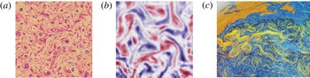
Examples of ideal and quasi-2D fluid turbulence that emphasize the role of coherent vortex structures in thin layers: (a) numerical simulation of ideal 2D turbulence (vorticity) (Boffetta & Ecke Reference Boffetta and Ecke2012), (b) laboratory quasi-2D turbulence (vorticity) (Boffetta & Ecke Reference Boffetta and Ecke2012) and (c) Atlantic Gulf Stream eddies (streak image) (Sirah Reference Sirah2012).
So what is the difference between two-dimensional (2D) turbulence (Boffetta & Ecke Reference Boffetta and Ecke2012) and the more familiar three-dimensional (3D) version (Frisch Reference Frisch1995)? In 3D, when energy is injected at large scales, it is transferred on average to smaller scales in a forward cascade with energy dissipated at the smallest scales by viscous forces. If the spatial scales of forcing and dissipation are widely separated, energy is conserved at intermediate scales, leading to a $-5/3$
power-law relationship between energy and wavenumber. In 2D, this transfer of energy to small scales cannot occur due to an additional conservation law related to the condition in 2D that the vorticity contained within a spatial contour is conserved; the vorticity can only be rearranged in space but not increased or reduced as is possible in 3D. Thus, a characteristic of 2D turbulence is the persistence of vortical structures; see figure 1. The constraint on vorticity implies that the mean-square vorticity is transferred to small scales whereas the energy flow is inverse, i.e. it is transferred to large scales. This leads to a double cascade in 2D, with energy cascading towards scales larger than the forcing scale whereas the mean-square vorticity cascades towards smaller scales. In many circumstances, the ideal limits of 3D or 2D turbulence are not met and there is a bidirectional cascade where different transfer mechanisms dominate at different length scales and no inertial range may exist. The relationship between the ideal limits in 2D and 3D with a bidirectional cascade for thin but 3D layers is what we consider here.
$-5/3$
power-law relationship between energy and wavenumber. In 2D, this transfer of energy to small scales cannot occur due to an additional conservation law related to the condition in 2D that the vorticity contained within a spatial contour is conserved; the vorticity can only be rearranged in space but not increased or reduced as is possible in 3D. Thus, a characteristic of 2D turbulence is the persistence of vortical structures; see figure 1. The constraint on vorticity implies that the mean-square vorticity is transferred to small scales whereas the energy flow is inverse, i.e. it is transferred to large scales. This leads to a double cascade in 2D, with energy cascading towards scales larger than the forcing scale whereas the mean-square vorticity cascades towards smaller scales. In many circumstances, the ideal limits of 3D or 2D turbulence are not met and there is a bidirectional cascade where different transfer mechanisms dominate at different length scales and no inertial range may exist. The relationship between the ideal limits in 2D and 3D with a bidirectional cascade for thin but 3D layers is what we consider here.
2 Overview
Much research on 3D and 2D turbulence has focused on ideal isotropic homogeneous turbulence in the respective spatial dimensions. There is, however, a large amount of interesting physics in the anisotropic regime of 3D turbulence where one direction is suppressed compared with the other two degrees of freedom. This is the regime recently addressed by Benavides & Alexakis (Reference Benavides and Alexakis2017), which significantly extends earlier work exploring the crossover from 3D turbulence to 2D turbulence (Celani, Musacchio & Vincenzi Reference Celani, Musacchio and Vincenzi2010). Benavides and Alexakis numerically compute a model with highly resolved 2D components in the lateral direction coupled to a truncated single-mode vertical component. The system is forced on a lateral scale $\ell _{f}$
that is large compared with the vertical height
$\ell _{f}$
that is large compared with the vertical height $H$
. The control parameter is
$H$
. The control parameter is $Q=\ell _{f}/H$
, where larger values correspond to thinner, more 2D systems. The energy flux is computed and its behaviour as a function of
$Q=\ell _{f}/H$
, where larger values correspond to thinner, more 2D systems. The energy flux is computed and its behaviour as a function of $Q$
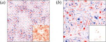
is considered. The resulting vorticity field reveals the quantitative feature of dominant vertical vorticity, as seen in figure 2. The insets show the 3D energy density and reflect the trend that as
$Q$
is considered. The resulting vorticity field reveals the quantitative feature of dominant vertical vorticity, as seen in figure 2. The insets show the 3D energy density and reflect the trend that as $Q$
is increased, the overall 3D energy density decreases, becoming highly singular in space for higher
$Q$
is increased, the overall 3D energy density decreases, becoming highly singular in space for higher $Q$
.
$Q$
.
Vertical vorticity and (insets) 3D energy density ${\mathcal{E}}$
for (a)
${\mathcal{E}}$
for (a) $\ell _{f}/H\sim 1$
, where vortices are weak and
$\ell _{f}/H\sim 1$
, where vortices are weak and ${\mathcal{E}}$
is fairly evenly distributed in space, and (b)
${\mathcal{E}}$
is fairly evenly distributed in space, and (b) $\ell _{f}/H\sim 10$
, where vortices are stronger and more spatially localized and
$\ell _{f}/H\sim 10$
, where vortices are stronger and more spatially localized and ${\mathcal{E}}$
is more spatially intermittent. After figure 7 in Benavides & Alexakis (Reference Benavides and Alexakis2017).
${\mathcal{E}}$
is more spatially intermittent. After figure 7 in Benavides & Alexakis (Reference Benavides and Alexakis2017).
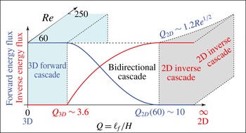
Schematic illustration of the behaviour of the normalized energy fluxes (forward and inverse) as a function of the degree of layer thinness $Q=\ell _{f}/H$
, adopted from Benavides & Alexakis (Reference Benavides and Alexakis2017, figures 1, 2 and 8). The ideal limits of 3D and 2D correspond to
$Q=\ell _{f}/H$
, adopted from Benavides & Alexakis (Reference Benavides and Alexakis2017, figures 1, 2 and 8). The ideal limits of 3D and 2D correspond to $Q=0$
and
$Q=0$
and $Q=\infty$
respectively. The transition to diminished forward energy flux at the expense of growing inverse energy flux occurs at
$Q=\infty$
respectively. The transition to diminished forward energy flux at the expense of growing inverse energy flux occurs at $Q_{3D}\sim 3.6$
, whereas the transition to no forward energy flux occurs at an
$Q_{3D}\sim 3.6$
, whereas the transition to no forward energy flux occurs at an $Re$
-dependent value where
$Re$
-dependent value where $Q_{2D}\sim 1.2Re^{1/2}$
. In between, energy flows in a bidirectional cascade where there is no inertial regime for either forward or inverse flux.
$Q_{2D}\sim 1.2Re^{1/2}$
. In between, energy flows in a bidirectional cascade where there is no inertial regime for either forward or inverse flux.
As $Q$
is varied, the forward energy flux characteristic of 3D turbulence and the 2D inverse energy flux behave in unexpected ways, namely they exhibit sharp transitions at specific values of
$Q$
is varied, the forward energy flux characteristic of 3D turbulence and the 2D inverse energy flux behave in unexpected ways, namely they exhibit sharp transitions at specific values of $Q$
. This behaviour is common in bifurcations in low-dimensional dynamical systems and in transitions from laminar to turbulent flow, but sharp transitions in turbulent flows are unusual. Benavides and Alexakis show that there is net inverse energy transfer that increases from zero at a well-defined value
$Q$
. This behaviour is common in bifurcations in low-dimensional dynamical systems and in transitions from laminar to turbulent flow, but sharp transitions in turbulent flows are unusual. Benavides and Alexakis show that there is net inverse energy transfer that increases from zero at a well-defined value $Q_{3D}\sim 3.6$
; see figure 3. At higher
$Q_{3D}\sim 3.6$
; see figure 3. At higher $Q$
, the 3D energy flux goes to zero sharply at a critical value of
$Q$
, the 3D energy flux goes to zero sharply at a critical value of $Q_{2D}$
that depends on the Reynolds number
$Q_{2D}$
that depends on the Reynolds number $Re$
of the flow. The empirically observed
$Re$
of the flow. The empirically observed $Re^{1/2}$
dependence of
$Re^{1/2}$
dependence of $Q_{2D}$
is consistent with scaling arguments by Benavides & Alexakis (Reference Benavides and Alexakis2017) and with a linear stability analysis of 2D flows with respect to 3D perturbations (Gallet & Doering Reference Gallet and Doering2015). Finally, Benavides & Alexakis (Reference Benavides and Alexakis2017) argue that the critical points should persist, as additional vertical modes are included in a fully resolved 3D numerical computation.
$Q_{2D}$
is consistent with scaling arguments by Benavides & Alexakis (Reference Benavides and Alexakis2017) and with a linear stability analysis of 2D flows with respect to 3D perturbations (Gallet & Doering Reference Gallet and Doering2015). Finally, Benavides & Alexakis (Reference Benavides and Alexakis2017) argue that the critical points should persist, as additional vertical modes are included in a fully resolved 3D numerical computation.
3 Future
The exciting results of Benavides & Alexakis (Reference Benavides and Alexakis2017) regarding the existence of sharp critical points in the crossover from 3D to 2D turbulent flows raise a number of questions that will be important in understanding how these results relate to large high- $Re$
turbulent flows in geophysical/astrophysical flows. In particular, the following questions arise. (i) To what degree are the transitions ‘sharp’ as resolution in
$Re$
turbulent flows in geophysical/astrophysical flows. In particular, the following questions arise. (i) To what degree are the transitions ‘sharp’ as resolution in $Q$
is increased? Even bifurcations in extremely well-controlled low-dimensional dynamical systems show some rounding due to experimental imperfections. Could the apparent
$Q$
is increased? Even bifurcations in extremely well-controlled low-dimensional dynamical systems show some rounding due to experimental imperfections. Could the apparent $(Q_{2D}-Q)^{2}$
dependence near the second critical point be instead rounding due to noise? (ii) What is the nature of the bidirectional cascades in which both forward and inverse energy transfer compete and the forward enstrophy cascade emerges? Can these cascades be inertial for sufficient scale separation between the critical points? (iii) Would a more realistic 3D model of thin layer flows preserve the nature of the critical points, as argued by Benavides & Alexakis (Reference Benavides and Alexakis2017), or would more degrees of freedom broaden the transitions (see also the question of sharpness above). The results of Benavides & Alexakis (Reference Benavides and Alexakis2017) raise numerous exciting questions as scientists attempt to extend idealized fluid experiments in the laboratory or in direct numerical simulations to real physical systems in nature such as the atmosphere and the ocean. The future continues to hold a wide range of challenges in understanding the roles of forcing scale, layer thickness, Reynolds number and body-force constraints such as magnetic field or rotation, to name just a few.
$(Q_{2D}-Q)^{2}$
dependence near the second critical point be instead rounding due to noise? (ii) What is the nature of the bidirectional cascades in which both forward and inverse energy transfer compete and the forward enstrophy cascade emerges? Can these cascades be inertial for sufficient scale separation between the critical points? (iii) Would a more realistic 3D model of thin layer flows preserve the nature of the critical points, as argued by Benavides & Alexakis (Reference Benavides and Alexakis2017), or would more degrees of freedom broaden the transitions (see also the question of sharpness above). The results of Benavides & Alexakis (Reference Benavides and Alexakis2017) raise numerous exciting questions as scientists attempt to extend idealized fluid experiments in the laboratory or in direct numerical simulations to real physical systems in nature such as the atmosphere and the ocean. The future continues to hold a wide range of challenges in understanding the roles of forcing scale, layer thickness, Reynolds number and body-force constraints such as magnetic field or rotation, to name just a few.