





1. Introduction
Viscoplastic materials behave as rigid solids when the applied stress is below a critical value and as fluids once that threshold is exceeded (Balmforth, Frigaard & Ovarlez Reference Balmforth, Frigaard and Ovarlez2014). As such, small gas bubbles which generate small buoyancy forces tend to become trapped in these materials during preparation and processing flows, intentionally or otherwise. Our concern here is with gas bubbles that arise from bacterial digestive processes within yield-stress media, i.e. bubbles that form and grow in situ. As they grow, the buoyancy force eventually overcomes restraining forces from the yield stress and the bubbles start to rise. This may happen within naturally formed ‘muck’ at the bottom of lakes and ponds, or as a result of industrial activity. In either case, a concern is the contribution to greenhouse gas emissions and similar negative environmental effects. Hence, these effects need to be quantified.
Our specific motivation comes from bubble trapping and release in oil sands tailings ponds (Small et al. Reference Small, Cho, Hashisho and Ulrich2015; He et al. Reference He2024). These large ponds contain tailings tens of metres deep and extend over many square kilometres. The tailings are colloidal suspensions that stratify in the pond as a result of solids settling. Larger solids fall through the liquid, but particles in the sub-20 μm range have body forces typically dominated by attractive colloidal forces, hence forming a yield-stress material. The rheology may be estimated from model correlations (Wells & Kaminsky Reference Wells and Kaminsky2015), from laboratory testing (e.g. Derakhshandeh Reference Derakhshandeh2016; Piette et al. Reference Piette, Moud, Poisson, Derakhshandeh, Hudson and Hatzikiriakos2022) or eventually from micro-mechanical models (Kapur et al. Reference Kapur, Scales, Boger and Healy1997; Scales et al. Reference Scales, Johnson, Healy and Kapur1998); see also (Wang et al. Reference Wang, Harbottle, Liu and Xu2014). In situ the density, solids content (clays, fines and coarse sand), clay-to-water ratio and yield stress will all stratify depthwise (Hajieghrary & Frigaard Reference Hajieghrary and Frigaard2024). However, this stratification occurs on length scales long with respect to bubble size, making the approximation of a bubble in uniform yield-stress fluid reasonable.
Residual bitumen and naphtha are digested within the ponds, generating $\text{CO}_2$
and
$\text{CO}_2$
and $\text{CH}_4$
, eventually forming bubbles, observed at the pond surface. Various fluid mechanical aspects of the process have been studied, such as ebullition, mixing and entrainment across interfaces (Lawrence, Tedford & Pieters Reference Lawrence, Tedford and Pieters2016; Tedford et al. Reference Tedford, Zhao, Olsthoorn, Pieters and Lawrence2019; Zhao et al. Reference Zhao, Tedford, Zare, Frigaard and Lawrence2022; Zare, Frigaard & Lawrence Reference Zare, Frigaard and Lawrence2024), all with a view to better managing/controlling process impacts. Here our focus is on a different problem: understanding the onset of bubble motion, i.e. trapping and release.
$\text{CH}_4$
, eventually forming bubbles, observed at the pond surface. Various fluid mechanical aspects of the process have been studied, such as ebullition, mixing and entrainment across interfaces (Lawrence, Tedford & Pieters Reference Lawrence, Tedford and Pieters2016; Tedford et al. Reference Tedford, Zhao, Olsthoorn, Pieters and Lawrence2019; Zhao et al. Reference Zhao, Tedford, Zare, Frigaard and Lawrence2022; Zare, Frigaard & Lawrence Reference Zare, Frigaard and Lawrence2024), all with a view to better managing/controlling process impacts. Here our focus is on a different problem: understanding the onset of bubble motion, i.e. trapping and release.
Quantifying the onset of motion of a bubble trapped in a yield-stress fluid is central to predicting gas emissions. The theoretical foundation for this problem was established by Dubash & Frigaard (Reference Dubash and Frigaard2004), who formulated the mobility flow problem and defined the critical yield number, $Y_c$
, marking the onset of bubble motion. Putz & Frigaard (Reference Putz and Frigaard2010) and Chaparian & Frigaard (Reference Chaparian and Frigaard2017) extended this approach to rigid particles settling in a yield-stress fluid, using resistance and mobility formulations, and exploring the limiting energy balances near
$Y_c$
, marking the onset of bubble motion. Putz & Frigaard (Reference Putz and Frigaard2010) and Chaparian & Frigaard (Reference Chaparian and Frigaard2017) extended this approach to rigid particles settling in a yield-stress fluid, using resistance and mobility formulations, and exploring the limiting energy balances near $Y_c$
. These analyses assumed a homogeneous Bingham fluid rheology, although all simple yield-stress fluids give the same
$Y_c$
. These analyses assumed a homogeneous Bingham fluid rheology, although all simple yield-stress fluids give the same $Y_c$
. Later, Pourzahedi et al. (Reference Pourzahedi, Chaparian, Roustaei and Frigaard2022) used high-resolution augmented-Lagrangian (AL) simulations to compute
$Y_c$
. Later, Pourzahedi et al. (Reference Pourzahedi, Chaparian, Roustaei and Frigaard2022) used high-resolution augmented-Lagrangian (AL) simulations to compute $Y_c$
for single bubbles of varying aspect ratio and surface tension, providing benchmark data for the present study. The first direct experimental study of flow onset (Daneshi & Frigaard Reference Daneshi and Frigaard2023) revealed changes in
$Y_c$
for single bubbles of varying aspect ratio and surface tension, providing benchmark data for the present study. The first direct experimental study of flow onset (Daneshi & Frigaard Reference Daneshi and Frigaard2023) revealed changes in $Y_c$
with bubble shape that were qualitatively consistent with those in Pourzahedi et al. (Reference Pourzahedi, Chaparian, Roustaei and Frigaard2022). With a view to application, where many bubbles are present in a tailings pond, bubble clouds were studied computationally in two dimensions by Chaparian & Frigaard (Reference Chaparian and Frigaard2021) and experimentally by Daneshi & Frigaard (Reference Daneshi and Frigaard2024), who examined the sensitivity of yielding/onset to bubble geometry, distribution and volume (area) fraction.
$Y_c$
with bubble shape that were qualitatively consistent with those in Pourzahedi et al. (Reference Pourzahedi, Chaparian, Roustaei and Frigaard2022). With a view to application, where many bubbles are present in a tailings pond, bubble clouds were studied computationally in two dimensions by Chaparian & Frigaard (Reference Chaparian and Frigaard2021) and experimentally by Daneshi & Frigaard (Reference Daneshi and Frigaard2024), who examined the sensitivity of yielding/onset to bubble geometry, distribution and volume (area) fraction.
While the above studies represented a logical progression in developing our understanding, they were based on the idealisation of randomly distributed bubbles in an inelastic viscoplastic liquid, at varying (likely low) volume fractions. Experimental insight has slowly chipped away at this image, leading to the current study. First was the observation that the computed steady rise shapes of bubbles in ideal viscoplastic fluids (Tsamopoulos et al. Reference Tsamopoulos, Dimakopoulos, Chatzidai, Karapetsas and Pavlidis2008; Dimakopoulos, Pavlidis & Tsamopoulos Reference Dimakopoulos, Pavlidis and Tsamopoulos2013) did not produce experimentally observed tail shapes and wake patterns. These shapes and effects were found only more recently by Moschopoulos et al. (Reference Moschopoulos, Spyridakis, Varchanis, Dimakopoulos and Tsamopoulos2021), who considered elastoviscoplastic (EVP) constitutive laws as the basis of their study.
Second was the observation that experimental repeatability using fluids such as Carbopol often required the fluids to be re-sheared/mixed between bubble releases. In particular, waiting for typical (viscoelastic) relaxation times did not remove the ‘memory’ of previous bubbles. Thus, resetting the fluid has been a common feature of many experimental bubble studies (Dubash & Frigaard Reference Dubash and Frigaard2007; Sikorski, Tabuteau & de Bruyn Reference Sikorski, Tabuteau and de Bruyn2009; Lopez et al. Reference Lopez, Naccache and de Souza Mendes2018; Wang et al. Reference Wang, Lou, Sun, Pan, Zhao and Liu2019), and also earlier in the context of studying settling particles (Atapattu, Chhabra & Uhlherr Reference Atapattu, Chhabra and Uhlherr1995; Gheissary & Van Den Brule Reference Gheissary and Van Den Brule1996). While initially these effects have been seen as an experimental inconvenience, later it has become apparent that they contain many interesting and important phenomena. Zare & Frigaard (Reference Zare and Frigaard2018) studied gas invasion into a column of Carbopol, driven under pressure through a nozzle. The bubble volume was not preset, but determined by a break-off process, influenced by the fluid rheology close to the nozzle. It was observed that the bubbles that formed/invaded after the initial bubble were consistently smaller than the first bubble, but also travelled upwards faster. This is consistent with the notion that the shearing in some way has ‘damaged’ the surrounding fluid. In earlier work, Mougin, Magnin & Piau (Reference Mougin, Magnin and Piau2012) showed that successive bubbles effectively sheared a confined channel through the fluid, outside of which there was little deformation. In an elegant experiment, Lopez et al. (Reference Lopez, Naccache and de Souza Mendes2018) sheared their fluid by drawing a solid rod through it, at an angle to the vertical. Remarkably, subsequent released bubbles translated along the path where the rod had been.
Inspired by Mougin et al. (Reference Mougin, Magnin and Piau2012) and Lopez et al. (Reference Lopez, Naccache and de Souza Mendes2018), in Zare, Daneshi & Frigaard (Reference Zare, Daneshi and Frigaard2021) we further explored the effects of non-uniform rheology on an actual bubble flow. Essentially, this meant ignoring exactly how the fluid became ‘damaged’ (i.e. rheologically), and looking at bubble dynamics in model two-liquid systems: a background yield-stress fluid (Bingham) and a damaged Newtonian layer of smaller viscosity. Using transient two-dimensional (2-D) computations and a regularisation method, bubbles released close to the damaged layer were found to approach the layer, become enveloped in it and travel upwards within the layer, at accelerated speeds and often elongating. Experiments confirmed these phenomena. Inclined damaged channels/pathways were also studied, computationally and experimentally, showing that bubbles could translate laterally even along strongly inclined damaged channels.
Around this time, we also became aware of field studies (Bussmann et al. Reference Bussmann, Schlömer, Schlüter and Wessels2011; Zhao et al. Reference Zhao, Tedford, Zare and Lawrence2021), where ‘pockmarks’ were observed in a sediment layer between a clear water cap and tailings suspension below. These circular holes are believed to be venting structures for the bubbles below. In the images of Zhao et al. (Reference Zhao, Tedford, Zare and Lawrence2021) the holes appear as entrances to a watery tunnel below, as was subsequently studied in the laboratory (Zhao et al. Reference Zhao, Tedford, Zare, Frigaard and Lawrence2022). This and the aforementioned studies in Zare et al. (Reference Zare, Daneshi and Frigaard2021) led to a reappraisal of the supposed subsurface bubble dynamics. Even if the initially nucleated bubbles are dispersed approximately uniformly and grow independently, it seemed likely that the release of bubbles and the paths followed to the surface would be influenced by the stress history of adjacent old pathways, i.e. promoting lateral migration and joining of pathways. The pockmarks and underlying tunnels may be indicators of a rootlike structure of bubble paths to the surface, repeatedly exiting through the same pockmarks.
This hypothesised structure has led to our current interest to quantify better the influence of adjacent damaged pathways on bubble release and passage. On release from entrapment there is an interest to assess the degree to which bubbles approach a damaged path. Recently, we studied this question experimentally (Goral & Frigaard Reference Goral and Frigaard2025), creating a 2-D ‘damaged layer’ by mechanically inserting a plate into and withdrawing it from a yield-stress-fluid bath, then releasing bubbles at different distances from the layer. The released bubbles were observed to migrate preferentially towards the damaged layer, as could be fitted by a simple toy model.
Regarding the actual bubble release, if an adjacent path results in a higher $Y_c$
value than in a uniform liquid, then bubbles will mobilise at smaller size. These in turn will create their own stress histories affecting further bubbles. Therefore, understanding how proximity affects
$Y_c$
value than in a uniform liquid, then bubbles will mobilise at smaller size. These in turn will create their own stress histories affecting further bubbles. Therefore, understanding how proximity affects $Y_c$
is of key importance in assessing the growing influence of damaged pathways. This is the topic of this paper. We determine the onset conditions for a single bubble rising in a damaged viscoplastic fluid, using an AL formulation. Section 2 presents the problem definition and governing equations. Section 3 outlines the numerical implementation and § 4 discusses the effects of offset distance, bubble aspect ratio, surface tension and viscosity ratio on the critical yield number
$Y_c$
is of key importance in assessing the growing influence of damaged pathways. This is the topic of this paper. We determine the onset conditions for a single bubble rising in a damaged viscoplastic fluid, using an AL formulation. Section 2 presents the problem definition and governing equations. Section 3 outlines the numerical implementation and § 4 discusses the effects of offset distance, bubble aspect ratio, surface tension and viscosity ratio on the critical yield number $Y_c$
, relative to the homogeneous fluid limit. We also explore the size of horizontal bubble velocities, affected by the damaged path.
$Y_c$
, relative to the homogeneous fluid limit. We also explore the size of horizontal bubble velocities, affected by the damaged path.
Throughout the paper we use a Bingham model for the viscoplastic fluid. The actual yield limit is independent of the post-yield rheology for all simple yield-stress fluids where the von Mises criterion is used (i.e. Herschel–Bulkley, Bingham, Casson, etc.). However, elastic effects are present in flow onset experiments, as in Daneshi & Frigaard (Reference Daneshi and Frigaard2024), and EVP model formulations are now more readily available (Moschopoulos et al. Reference Moschopoulos, Spyridakis, Varchanis, Dimakopoulos and Tsamopoulos2021; Esposito, Dimakopoulos & Tsamopoulos Reference Esposito, Dimakopoulos and Tsamopoulos2025). Our reason for avoiding these models is twofold. Firstly, popular models such as that of Saramito (Reference Saramito2007, Reference Saramito2009) are built around a description of viscoelastic flow, rather than elastic deformation and yielding. Secondly, the onset problem for an EVP fluid is not well defined. As found in Daneshi & Frigaard (Reference Daneshi and Frigaard2024), an initial bubble shape deforms elastically and significantly before eventually yielding plastically and flowing. The sensitivity of the deformation path to the initial bubble shape and the timeframe allowed for elastic deformation are two additional variables, not understood. Simple yield-stress fluids have a clear well-defined limit $Y_c$
for each shape. The computed (inelastic)
$Y_c$
for each shape. The computed (inelastic) $Y_c$
is likely a lower bound for associated EVP fluids, with small elastic effects, but a general theory is lacking.
$Y_c$
is likely a lower bound for associated EVP fluids, with small elastic effects, but a general theory is lacking.
2. Problem statement
We explore the yield limit of a bubble rising in a non-uniform viscoplastic fluid domain. The scenario considered is that a narrow vertical region close to the bubble has been damaged by the motion of a previous bubble. The aim is to quantify the influence of the damaged path on flow onset in a simplified model setting, so that insights can be gained regarding the industrially relevant flows described in § 1.
Our model problem uses three simplifying assumptions. First, the yield-stress fluid is modelled as a Bingham fluid, discussed above. Second, the damaged path is modelled as a vertical Newtonian channel of width equal to the bubble diameter, embedded within the viscoplastic fluid. This represents a simplified frozen heterogeneity approximation of the weakened fluid structure created by previous bubble motion. The model isolates the mechanical influence of a pre-existing pathway rather than attempting to simulate the rheological processes responsible for its formation or recovery. The choice of a Newtonian layer, as opposed to yield-stress fluid of lower yield stress is for simplicity. Lastly, we adopt a 2-D planar model, which speeds computation. An axisymmetric bubble with damaged layer would imply a damaged cylinder around the bubble, which is not representative. Hence, an expensive fully three-dimensional (3-D) computation would be the next most complete model, which is beyond the scope here. A discussion of the applicability of our 2-D results is given in § 5.
The computational domain, denoted by $\varOmega$
, includes the entire fluid region: the bubble
$\varOmega$
, includes the entire fluid region: the bubble $X$
, the surrounding Newtonian layer and the bulk viscoplastic material. The outer boundary of the domain is
$X$
, the surrounding Newtonian layer and the bulk viscoplastic material. The outer boundary of the domain is $\partial \varOmega$
, and the bubble boundary is denoted by
$\partial \varOmega$
, and the bubble boundary is denoted by $\partial X$
(see figure 1). The bubble is assumed to have a fixed elliptical shape with aspect ratio defined as the ratio of bubble height to width:
$\partial X$
(see figure 1). The bubble is assumed to have a fixed elliptical shape with aspect ratio defined as the ratio of bubble height to width: $\chi \lt 1$
corresponds to horizontally flattened bubbles (which we here refer to as oblate),
$\chi \lt 1$
corresponds to horizontally flattened bubbles (which we here refer to as oblate), $\chi = 1$
to circular bubbles and
$\chi = 1$
to circular bubbles and $\chi \gt 1$
to vertically elongated bubbles (which we here refer to as prolate). Here, oblate and prolate refer only to the orientation of the 2-D ellipse, and not to 3-D shapes. In all cases, due to the scaling, the area of the bubble equals
$\chi \gt 1$
to vertically elongated bubbles (which we here refer to as prolate). Here, oblate and prolate refer only to the orientation of the 2-D ellipse, and not to 3-D shapes. In all cases, due to the scaling, the area of the bubble equals $\pi$
, meaning that the major and minor axes have lengths
$\pi$
, meaning that the major and minor axes have lengths $2\sqrt {\chi }$
and
$2\sqrt {\chi }$
and $2/\sqrt {\chi }$
(or vice versa). The flow is considered in the Stokes regime, where inertia is negligible, since our questions are regarding onset of motion. We first formulate the problem in a natural way, using the buoyancy force of the bubble as the stress scale that drives the motion (mobility problem, [M]). Later we reformulate the problem as an equivalent resistance problem [R], where the bubble’s mean motion is prescribed, which has some computational advantages.
$2/\sqrt {\chi }$
(or vice versa). The flow is considered in the Stokes regime, where inertia is negligible, since our questions are regarding onset of motion. We first formulate the problem in a natural way, using the buoyancy force of the bubble as the stress scale that drives the motion (mobility problem, [M]). Later we reformulate the problem as an equivalent resistance problem [R], where the bubble’s mean motion is prescribed, which has some computational advantages.
Schematic of the problem domain.

2.1. Governing equations
The Stokes equations for the fluid region outside the bubble are
 \begin{align} \boldsymbol{\nabla }\boldsymbol{\cdot }\hat {\boldsymbol{\sigma }} - \hat {\rho }_f \hat {g} \boldsymbol{e}_y &= 0 \quad \text{in } \varOmega \setminus \overline {X} ,\end{align}
 \begin{align} \boldsymbol{\nabla }\boldsymbol{\cdot }\hat {\boldsymbol{u}} &= 0 \quad \text{in } \varOmega \setminus \overline {X}. \end{align}
Here, $\hat {\boldsymbol{\sigma }}$
is the Cauchy stress tensor,
$\hat {\boldsymbol{\sigma }}$
is the Cauchy stress tensor, $\hat {\rho }_f$
is the fluid density,
$\hat {\rho }_f$
is the fluid density, $\hat {g}$
is the gravitational acceleration and
$\hat {g}$
is the gravitational acceleration and $\hat {\boldsymbol{u}}$
is the fluid velocity in the domain
$\hat {\boldsymbol{u}}$
is the fluid velocity in the domain $\varOmega \setminus \overline {X}$
. Dimensional quantities are denoted by the accent
$\varOmega \setminus \overline {X}$
. Dimensional quantities are denoted by the accent $\hat {\boldsymbol{\cdot }}$
, while non-dimensional variables appear without it. The Cauchy stress tensor is expressed as
$\hat {\boldsymbol{\cdot }}$
, while non-dimensional variables appear without it. The Cauchy stress tensor is expressed as
 \begin{align} \hat {\boldsymbol{\sigma }} = -\hat {p} \boldsymbol{\delta } + \hat {\boldsymbol{\tau }}, \end{align}
where $\hat {p}$
is the pressure,
$\hat {p}$
is the pressure, $\hat {\boldsymbol{\tau }}$
is the deviatoric stress tensor and
$\hat {\boldsymbol{\tau }}$
is the deviatoric stress tensor and $\boldsymbol{\delta }$
is the Kronecker delta.
$\boldsymbol{\delta }$
is the Kronecker delta.
As we focus on the yield limit of the flow, the viscous behaviour after yielding becomes of secondary interest. Therefore, we adopt the simplest constitutive model for the viscoplastic region, the Bingham fluid model:
 \begin{align} \hat {\boldsymbol{\tau }} = \begin{cases} \left ( \hat {\mu }_p + \displaystyle {\frac {\hat {\tau }_y}{\|\hat {{\dot \gamma }}(\hat {\boldsymbol{u}})\|}} \right ) {\hat {\dot \gamma }}(\hat {\boldsymbol{u}}), & \text{if } \|\hat {\tau }\| \gt \hat {\tau }_y, \\ {\hat {\dot \gamma }}(\hat {\boldsymbol{u}}) = 0, & \text{if } \|\hat {\tau }\| \leqslant \hat {\tau }_y ,\end{cases} \end{align}
where $\hat {\mu }_p$
is the plastic viscosity,
$\hat {\mu }_p$
is the plastic viscosity, $\hat {\tau }_y$
is the yield stress and
$\hat {\tau }_y$
is the yield stress and $\hat {{\dot \gamma }}$
is the rate-of-strain tensor associated with the velocity field
$\hat {{\dot \gamma }}$
is the rate-of-strain tensor associated with the velocity field $\hat {\boldsymbol{u}}$
. The rate-of-strain tensor is given component-wise by
$\hat {\boldsymbol{u}}$
. The rate-of-strain tensor is given component-wise by
 \begin{align} \hat {{\dot \gamma }}_{\textit{ij}}(\hat {\boldsymbol{u}}) = \frac {\partial \hat {u}_i}{\partial \hat {x}_j} + \frac {\partial \hat {u}_j}{\partial \hat {x}_i}. \end{align}
The appropriate norms of the rate-of-strain tensor $\hat {\boldsymbol{{\dot \gamma }}}$
and deviatoric stress tensor
$\hat {\boldsymbol{{\dot \gamma }}}$
and deviatoric stress tensor $\hat {\boldsymbol{\tau }}$
are
$\hat {\boldsymbol{\tau }}$
are
 \begin{align} \|\hat {{\dot \gamma }}(\hat {\boldsymbol{u}})\| = \sqrt {\frac {1}{2} \sum _{\textit{ij}} \hat {{\dot \gamma }}_{\textit{ij}}^2(\hat {\boldsymbol{u}})} \quad \text{and} \quad \|\hat {\tau }(\hat {\boldsymbol{u}})\| = \sqrt {\frac {1}{2} \sum _{\textit{ij}} \hat {\tau }_{\textit{ij}}^2(\hat {\boldsymbol{u}})}, \end{align}
associated with the tensor inner product $\boldsymbol{a}:\boldsymbol{b} = ({1}/{2}) \sum _{\textit{ij}} a_{\textit{ij}}b_{\textit{ij}}$
. In the damaged region, we assume the material behaves as a Newtonian fluid. The stress is linearly related to the strain rate:
$\boldsymbol{a}:\boldsymbol{b} = ({1}/{2}) \sum _{\textit{ij}} a_{\textit{ij}}b_{\textit{ij}}$
. In the damaged region, we assume the material behaves as a Newtonian fluid. The stress is linearly related to the strain rate:
 \begin{align} \hat {\boldsymbol{\tau }} = \hat {\mu }_N \hat {\dot \gamma }(\hat {\boldsymbol{u}}), \end{align}
where $\hat {\mu }_N$
is the viscosity of the Newtonian fluid in the damaged region. Regarding the boundary conditions, in the far field, we specify
$\hat {\mu }_N$
is the viscosity of the Newtonian fluid in the damaged region. Regarding the boundary conditions, in the far field, we specify
 \begin{align} \hat {\boldsymbol u} =0 \quad \text{on } \partial \varOmega . \end{align}
At the bubble surface $ \partial X$
, the fluid velocity is continuous. As the gas phase has negligible viscosity relative to the surrounding yield-stress fluid, the tangential component of stress is assumed to vanish at the surface, corresponding to a free-slip condition:
$ \partial X$
, the fluid velocity is continuous. As the gas phase has negligible viscosity relative to the surrounding yield-stress fluid, the tangential component of stress is assumed to vanish at the surface, corresponding to a free-slip condition:
 \begin{equation} (\hat {\boldsymbol{\tau }} \boldsymbol{\cdot }\boldsymbol{n}) \boldsymbol{\cdot }\boldsymbol{t} = 0 \quad \text{on } \partial X, \end{equation}
where $ \boldsymbol{n}$
and
$ \boldsymbol{n}$
and $ \boldsymbol{t}$
denote the outward unit normal and tangential vectors to the bubble surface, respectively. This condition ensures that no shear stress is transmitted across the bubble boundary.
$ \boldsymbol{t}$
denote the outward unit normal and tangential vectors to the bubble surface, respectively. This condition ensures that no shear stress is transmitted across the bubble boundary.
In contrast, the normal component of the stress must balance the internal gas pressure and the capillary traction due to surface tension, expressed as
 \begin{equation} \hat p_b = \hat p - (\hat {\boldsymbol{\tau }} \boldsymbol{\cdot }\boldsymbol{n}) \boldsymbol{\cdot }\boldsymbol{n} + \frac {\hat \gamma }{\hat \kappa } \quad \text{on } \partial X, \end{equation}
where $ \hat p_b$
is the pressure inside the bubble,
$ \hat p_b$
is the pressure inside the bubble, $ \hat {\gamma }$
is the surface tension coefficient and
$ \hat {\gamma }$
is the surface tension coefficient and $ \hat \kappa$
denotes the local curvature of the interface. This relation describes the pressure jump across the bubble surface resulting from capillary forces.
$ \hat \kappa$
denotes the local curvature of the interface. This relation describes the pressure jump across the bubble surface resulting from capillary forces.
2.2. Dimensionless formulation
2.2.1. Mobility scaling
To scale the problem, we select a characteristic length scale $ \hat {R}$
based on the bubble radius. The characteristic velocity scale is determined by balancing the buoyancy force with viscous resistance in the viscoplastic fluids, leading to
$ \hat {R}$
based on the bubble radius. The characteristic velocity scale is determined by balancing the buoyancy force with viscous resistance in the viscoplastic fluids, leading to
 \begin{equation} \hat {U}_b = \frac {(\hat {\rho }_f - \hat {\rho }_g) \hat {g} \hat {R}^2}{\hat {\mu }_p}. \end{equation}
Stresses are scaled by the viscous stress scale $ \hat {\mu }_p \hat {U}_b / \hat {R}$
, which is equivalent to the buoyancy stress scale
$ \hat {\mu }_p \hat {U}_b / \hat {R}$
, which is equivalent to the buoyancy stress scale $ (\hat {\rho }_f - \hat {\rho }_g) \hat {g} \hat {R}$
. Using these scales, the dimensionless governing equations take the form
$ (\hat {\rho }_f - \hat {\rho }_g) \hat {g} \hat {R}$
. Using these scales, the dimensionless governing equations take the form
 \begin{align} \boldsymbol{\nabla }\boldsymbol{\cdot }\boldsymbol{\sigma } - \frac {1}{1 - \rho _r} \boldsymbol{e}_g &= 0, \quad \text{in } \varOmega \setminus \overline {X}, \end{align}
 \begin{align} \boldsymbol{\nabla }\boldsymbol{\cdot }\boldsymbol{u} &= 0, \quad \text{in } \varOmega \setminus \overline {X}, \end{align}
where $ \rho _r = \hat {\rho }_g / \hat {\rho }_f$
is the density ratio. Since typically
$ \rho _r = \hat {\rho }_g / \hat {\rho }_f$
is the density ratio. Since typically $ \hat {\rho }_g \ll \hat {\rho }_f$
, we have
$ \hat {\rho }_g \ll \hat {\rho }_f$
, we have $ \rho _r \approx 0$
.
$ \rho _r \approx 0$
.
The dimensionless constitutive law for the Bingham flow is given by
 \begin{align} \boldsymbol{\tau } = \begin{cases} \left ( 1 + \displaystyle \frac {Y}{\|\dot {\boldsymbol{\gamma }}(\boldsymbol{u})\|} \right ) \dot {\boldsymbol{\gamma }}(\boldsymbol{u}), & \text{iff } \|\boldsymbol{\tau }\| \gt Y, \\ \dot {\boldsymbol{\gamma }}(\boldsymbol{u}) = 0, & \text{iff } \|\boldsymbol{\tau }\| \leqslant Y, \end{cases} \end{align}
where $ Y={\hat {\tau }_y \hat {R}}/{\hat {\mu }_p \hat {U}_b}$
is the dimensionless yield number.
$ Y={\hat {\tau }_y \hat {R}}/{\hat {\mu }_p \hat {U}_b}$
is the dimensionless yield number.
For the Newtonian region, the constitutive law simplifies to
 \begin{equation} \boldsymbol{\tau } = \mu \dot {\boldsymbol{\gamma }}(\boldsymbol{u}), \end{equation}
where $ \mu = {\hat {\mu }_N}/{\hat {\mu }_p}$
is the viscosity ratio. Generally,
$ \mu = {\hat {\mu }_N}/{\hat {\mu }_p}$
is the viscosity ratio. Generally, $\mu \lt 1$
is assumed, implying that the damaged region is less viscous than the surrounding viscoplastic medium.
$\mu \lt 1$
is assumed, implying that the damaged region is less viscous than the surrounding viscoplastic medium.
2.2.2. Mobility variational formulation
To derive the mobility problem [M], we first introduce $\mathcal V_M$
as the space of admissible velocity fields, consisting of divergence-free vector fields that vanish on the far-field boundary:
$\mathcal V_M$
as the space of admissible velocity fields, consisting of divergence-free vector fields that vanish on the far-field boundary:
 \begin{equation} \mathcal V_{M} = \left \{ \boldsymbol{v}: \boldsymbol{\nabla }\boldsymbol{\cdot }\boldsymbol{v} = 0 \text{ in } \varOmega \setminus \overline {X}, \quad \boldsymbol{v} = 0 \text{ on } \partial \varOmega \setminus \partial X \right \}. \end{equation}
Using tools from convex analysis (see e.g. Ekeland & Temam Reference Ekeland and Temam1999), the mobility problem can be formulated as a minimisation principle. The solution velocity $\boldsymbol{u} \in \mathcal V_M$
is the unique minimiser of the functional
$\boldsymbol{u} \in \mathcal V_M$
is the unique minimiser of the functional
 \begin{equation} J_M({\boldsymbol v}) = \frac {1}{2} a({\boldsymbol v},{\boldsymbol v}) + Y j({\boldsymbol v}) - L_M({\boldsymbol v}) - T_M({\boldsymbol v}), \qquad {\boldsymbol v} \in \mathcal V_M, \end{equation}
where the functionals are defined as
 \begin{align} a({\boldsymbol u},{\boldsymbol v}) &= a_B({\boldsymbol u},{\boldsymbol v}) + \mu a_N({\boldsymbol u},{\boldsymbol v}) , \nonumber \\ &=\int \limits _{\varOmega _B} {{\dot \gamma }}(\boldsymbol{u}):{{\dot \gamma }}(\boldsymbol{v})\,\textrm {d} \boldsymbol{\varOmega } + \mu \int \limits _{\varOmega _N} {{\dot \gamma }}(\boldsymbol{u}):{{\dot \gamma }}(\boldsymbol{v})\,\textrm {d} \boldsymbol{\varOmega }, \end{align}
 \begin{align} j({\boldsymbol v}) &= \int \limits _{\varOmega _B} \|{\dot \gamma }(\boldsymbol{v})\|\,\textrm {d} \boldsymbol{\varOmega }, \end{align}
 \begin{align} L_M({\boldsymbol v}) &= -\frac {1}{1-\rho _r} \int \limits _{\varOmega \setminus \overline {X}}{\boldsymbol{v} \boldsymbol{\cdot }\boldsymbol e}_{g} \,\textrm {d} \boldsymbol{\varOmega }, \end{align}
 \begin{align} T_M({\boldsymbol v}) &= -\int \limits _{\partial X} \frac {\gamma _M}{\kappa }\boldsymbol v \boldsymbol{\cdot }\boldsymbol n_j \, \textrm {d} s . \end{align}
We have denoted the Bingham fluid domain by $\varOmega _B$
and the Newtonian damaged layer by
$\varOmega _B$
and the Newtonian damaged layer by $\varOmega _N$
, where
$\varOmega _N$
, where $\varOmega \setminus \overline {X} = \varOmega _B \cup \varOmega _N$
. The functionals
$\varOmega \setminus \overline {X} = \varOmega _B \cup \varOmega _N$
. The functionals $ a(v,v)$
and
$ a(v,v)$
and $ j(v)$
represent the effects of viscous and plastic dissipation within the fluid, respectively, whereas
$ j(v)$
represent the effects of viscous and plastic dissipation within the fluid, respectively, whereas $ L_M(v)$
and
$ L_M(v)$
and $ T_M(v)$
correspond to the work done by buoyancy and surface tension. The surface tension term is also scaled with the characteristic buoyancy stress, so that
$ T_M(v)$
correspond to the work done by buoyancy and surface tension. The surface tension term is also scaled with the characteristic buoyancy stress, so that
 \begin{equation} \gamma _M = \frac {\hat {\gamma }}{(\hat {\rho }_f - \hat {\rho }_g)\hat {g} \hat {R}^2}. \end{equation}
A dual variational principle can also be formulated in terms of the admissible stress tensor $ \tilde {\boldsymbol{\tau }}$
. If
$ \tilde {\boldsymbol{\tau }}$
. If $ \boldsymbol{u}$
is the minimiser of
$ \boldsymbol{u}$
is the minimiser of $ J_M$
, then the corresponding stress field
$ J_M$
, then the corresponding stress field $ \boldsymbol{\tau }$
maximises the functional
$ \boldsymbol{\tau }$
maximises the functional
 \begin{equation} I(\tilde {\boldsymbol{\tau }}) = \frac {1}{2} \int _{\varOmega \setminus \overline {X}} \big (\|\tilde {\boldsymbol{\tau }}\| - Y\big )_{+}^{2}\, \textrm {d} \varOmega , \end{equation}
where $ (\boldsymbol{\cdot })_+$
denotes the positive part.
$ (\boldsymbol{\cdot })_+$
denotes the positive part.
Generally, the primal and dual problems are linked through the following inequalities (originally derived by Prager (Reference Prager1954) for simpler flows):
 \begin{equation} I(\tilde {\boldsymbol{\tau }}) \;\leqslant \; I(\boldsymbol{\tau }) = J_M(\boldsymbol{u}) \;\leqslant \; J_M(\boldsymbol{v}). \end{equation}
Thus, the velocity solution $ \boldsymbol{u}$
uniquely minimises
$ \boldsymbol{u}$
uniquely minimises $ J_M$
over the admissible space
$ J_M$
over the admissible space $\mathcal V_M$
, while the associated stress field
$\mathcal V_M$
, while the associated stress field $ \boldsymbol{\tau }$
maximises
$ \boldsymbol{\tau }$
maximises $ I$
. For the exact solution, the difference between these two functionals vanishes, whereas for approximate admissible fields it remains strictly positive, known as the duality gap.
$ I$
. For the exact solution, the difference between these two functionals vanishes, whereas for approximate admissible fields it remains strictly positive, known as the duality gap.
Most computational methods are based on solving the velocity minimisation. This may be equivalently formulated as a variational inequality, i.e. $\boldsymbol{u} \in \mathcal V_M$
satisfies
$\boldsymbol{u} \in \mathcal V_M$
satisfies
 \begin{equation} a({\boldsymbol u},{\boldsymbol v}-{\boldsymbol u}) + Y [j({\boldsymbol v}) - j({\boldsymbol u}) ] \geqslant L_M({\boldsymbol v}-{\boldsymbol u}) + T_M({\boldsymbol v}-{\boldsymbol u}), \,\,\,\,\forall \boldsymbol{v} \in \mathcal V_M . \end{equation}
Lastly, the solution $\boldsymbol{u} \in \mathcal V_M$
satisfies the steady (mechanical) energy equation:
$\boldsymbol{u} \in \mathcal V_M$
satisfies the steady (mechanical) energy equation:
 \begin{equation} a({\boldsymbol u},{\boldsymbol u}) + Y j({\boldsymbol u}) = L_M({\boldsymbol u}) + T_M({\boldsymbol u}), \end{equation}
which is used in defining the yield limit.
2.2.3. Resistance scaling and formulation
In dealing with particle settling problems, a resistance formulation is often adopted, i.e. the particle motion is imposed and the resisting force calculated. This formulation is less natural for bubbles and droplets that may deform while moving. Indeed unlike rigid particles, where the velocity can be imposed directly on the boundary $\partial X$
as in Putz & Frigaard (Reference Putz and Frigaard2010), the bubble surface velocity is not easily determined. However, we shall see later that the resistance formulation has advantages in determining flow onset for specified interface shapes, where deformation of the interface with time is not a concern, i.e. because we determine a static limit.
$\partial X$
as in Putz & Frigaard (Reference Putz and Frigaard2010), the bubble surface velocity is not easily determined. However, we shall see later that the resistance formulation has advantages in determining flow onset for specified interface shapes, where deformation of the interface with time is not a concern, i.e. because we determine a static limit.
For the resistance formulation [R] we use the vertical component of the mean bubble velocity $\hat {U}_0$
, as velocity scale. Since the velocity field is divergence-free, the net volumetric flux across the entire domain
$\hat {U}_0$
, as velocity scale. Since the velocity field is divergence-free, the net volumetric flux across the entire domain $ \varOmega$
must be zero. Thus, the downward flux of the fluid domain must balance the upward motion of the bubble. This constraint allows us to express the mean bubble velocity in terms of the fluid velocity field:
$ \varOmega$
must be zero. Thus, the downward flux of the fluid domain must balance the upward motion of the bubble. This constraint allows us to express the mean bubble velocity in terms of the fluid velocity field:
 \begin{equation} \hat {U}_0 = -\frac {1}{\pi \hat {R}^2} \int _{\varOmega \setminus \overline {X}} \hat {\boldsymbol{u}} \boldsymbol{\cdot }\boldsymbol{e}_g \, \textrm {d} \varOmega . \end{equation}
On scaling velocities with $\hat {U}_0$
and lengths with
$\hat {U}_0$
and lengths with $\hat {R}$
, we see that the dimensionless velocity
$\hat {R}$
, we see that the dimensionless velocity $\boldsymbol{u}^*$
lies in the set
$\boldsymbol{u}^*$
lies in the set $ \mathcal{V}_R$
of admissible velocity fields:
$ \mathcal{V}_R$
of admissible velocity fields:
 \begin{equation} \mathcal{V}_{R}=\left\{ \boldsymbol{v}^*: \int \limits _{\varOmega \setminus \overline {X}} \boldsymbol{v}^* \boldsymbol{\cdot }\boldsymbol{e}_g \,\textrm {d} \varOmega =-\pi ; \,\,\boldsymbol{\boldsymbol{\nabla }} \boldsymbol{\cdot }\boldsymbol{v}^* = 0, \,\, \text{in } \varOmega \setminus \overline {X};\,\,\boldsymbol{v}^*=0 \text{ on }\partial \varOmega \right\} . \end{equation}
The solution $\boldsymbol{u}^* \in \mathcal{V}_R$
is the minimiser of
$\boldsymbol{u}^* \in \mathcal{V}_R$
is the minimiser of
 \begin{equation} J_R(\boldsymbol{v}^*) = \frac {1}{2} a(\boldsymbol{v}^*,\boldsymbol{v}^*) + B j(\boldsymbol{v}^*) - L_R(\boldsymbol{v}^*) - T_R(\boldsymbol{v}^*), \,\,\,\, \boldsymbol{v}^* \in \mathcal{V}_R, \end{equation}
where the linear functionals $ L_R(\boldsymbol{v}^*)$
and
$ L_R(\boldsymbol{v}^*)$
and $ T_R(\boldsymbol{v}^*)$
represent the effects of buoyancy and surface tension, respectively:
$ T_R(\boldsymbol{v}^*)$
represent the effects of buoyancy and surface tension, respectively:
 \begin{align} L_R(\boldsymbol{v}^*) &= - \frac {1}{1 - \rho _r} \frac {B}{Y} \int _{\varOmega \setminus \overline {X}} \boldsymbol{e}_g \boldsymbol{\cdot }\boldsymbol{v}^* \, \textrm {d}\varOmega , \end{align}
 \begin{align} T_R(\boldsymbol{v}^*) &= - \int _{\partial X} \frac {\gamma _R}{\kappa } \, \boldsymbol{v}^* \boldsymbol{\cdot }\boldsymbol{n} \, \textrm {d} S. \end{align}
Here, the non-dimensional Bingham number $ B$
and surface tension parameter
$ B$
and surface tension parameter $ \gamma _R$
are defined as
$ \gamma _R$
are defined as
 \begin{align} B &= \frac {\hat {\tau }_y \hat {R}}{\hat {\mu } \hat {U}_0}, \end{align}
 \begin{align} \gamma _R &= \frac {\hat {\gamma }}{\hat {\mu } \hat {U}_0}. \end{align}
As with the mobility formulation, the velocity minimisation can be written as a variational inequality. The mechanical energy balance in the resistance formulation is given by
 \begin{equation} a({\boldsymbol u}^*,{\boldsymbol u}^*) + B j({\boldsymbol u}^*) = L_R({\boldsymbol u}^*) + T_R({\boldsymbol u}^*), \end{equation}
for the solution $\boldsymbol{u}^* \in \mathcal V_R$
.
$\boldsymbol{u}^* \in \mathcal V_R$
.
2.3. Mapping between mobility and resistance formulations
The two formulations introduced differ in their choice of velocity scale. While the mobility formulation leads to an easier computational implementation, we will see below that the yield limit is defined by the ratio of two functionals that both approach zero in this limit. The resistance formulation avoids this feature. Thus, although we have used both formulations for computation, the resistance formulation has some advantage in computing the yield limit. The relationship between the Bingham number $ B$
and the yield number
$ B$
and the yield number $ Y$
is reflected in the ratio of the characteristic velocities used in each formulation:
$ Y$
is reflected in the ratio of the characteristic velocities used in each formulation:
 \begin{equation} \frac {B}{Y} = \frac {\hat {U}_b}{\hat {U}_0}. \end{equation}
Note that since the yield limit is defined by a stationary bubble, $\hat {U}_0 = 0$
, we see that
$\hat {U}_0 = 0$
, we see that $B \to \infty$
at flow onset.
$B \to \infty$
at flow onset.
To express the resistance formulation in terms of the mobility variables, we apply the scaling $ \boldsymbol{u}^* = ({\hat {U}_b}/{\hat {U}_0}) \boldsymbol{u}$
, where
$ \boldsymbol{u}^* = ({\hat {U}_b}/{\hat {U}_0}) \boldsymbol{u}$
, where $\boldsymbol{u}^* \in \mathcal V_R$
and
$\boldsymbol{u}^* \in \mathcal V_R$
and $\boldsymbol{u} \in \mathcal V_M$
. Using (2.27) and
$\boldsymbol{u} \in \mathcal V_M$
. Using (2.27) and
 \begin{equation} \gamma _R = \frac {B}{Y} \gamma _M, \end{equation}
we see that the energy equation in the resistance formulation is
 \begin{align} a(\boldsymbol{u}^*, \boldsymbol{u}^*) + B j(\boldsymbol{u}^*) &= \frac {B}{Y} [L_M(\boldsymbol{u}^*) + T_M(\boldsymbol{u}^*)], \end{align}
 \begin{align} \left (\frac {B}{Y}\right )^2 a(\boldsymbol{u}, \boldsymbol{u}) + B \left (\frac {B}{Y}\right ) j(\boldsymbol{u}) &= \left (\frac {B}{Y}\right )^2 [L_M(\boldsymbol{u}) + T_M(\boldsymbol{u})], \end{align}
which is (2.19).
2.4. Yield limit calculation
The yield limit of bubble motion is the conditions under which a bubble ceases to move in a viscoplastic fluid. This happens when $ Y$
exceeds a critical value
$ Y$
exceeds a critical value $ Y_{\text{c}}$
, and the material does not yield anywhere. Using the variational framework introduced earlier, following Dubash & Frigaard (Reference Dubash and Frigaard2004), assuming that
$ Y_{\text{c}}$
, and the material does not yield anywhere. Using the variational framework introduced earlier, following Dubash & Frigaard (Reference Dubash and Frigaard2004), assuming that ${\boldsymbol u} \neq 0$
:
${\boldsymbol u} \neq 0$
:
 \begin{align} 0 \leqslant a({\boldsymbol u},{\boldsymbol u}) & = L_M({\boldsymbol u}) + T_M({\boldsymbol u}) - Y j({\boldsymbol u}) = j({\boldsymbol u}) \left [ \frac {L_M({\boldsymbol u}) + T_M({\boldsymbol u})}{j({\boldsymbol u})} - Y \right ] \nonumber \\ & \leqslant j({\boldsymbol u}) \left [ \sup _{\boldsymbol v \in \mathcal V_M,\,\boldsymbol v \neq 0} \frac {L_M({\boldsymbol v}) + T_M({\boldsymbol v})}{j({\boldsymbol v})} - Y \right ] = j({\boldsymbol u}) [Y_c - Y], \end{align}
where $Y_c$
is defined by
$Y_c$
is defined by
 \begin{align} Y_c = \sup _{\boldsymbol v \in \mathcal V_M,\,\boldsymbol v \neq 0} \frac {L_M({\boldsymbol v}) + T_M({\boldsymbol v})}{j({\boldsymbol v})}. \end{align}
Having found $Y_c$
, in the limit
$Y_c$
, in the limit $ Y \rightarrow Y_c^-$
, it can be shown that
$ Y \rightarrow Y_c^-$
, it can be shown that
 \begin{align} a(\boldsymbol u,\boldsymbol u) &= \mathcal{O}\left((Y_c - Y)^2\right)\!, \end{align}
 \begin{align} j(\boldsymbol u) &= \mathcal{O}(Y_c - Y), \end{align}
and also that the viscous dissipation $a(\boldsymbol u,\boldsymbol u)$
decays at least one order of magnitude faster than the plastic dissipation term
$a(\boldsymbol u,\boldsymbol u)$
decays at least one order of magnitude faster than the plastic dissipation term $j(\boldsymbol u)$
.
$j(\boldsymbol u)$
.
Since (2.32) appears daunting to evaluate, an alternative is a simple and direct method of calculation, i.e. increase $Y$
from zero until the solution decays to zero, as (2.33) guarantees. Figure 2 shows the typical decay of these functionals as
$Y$
from zero until the solution decays to zero, as (2.33) guarantees. Figure 2 shows the typical decay of these functionals as $Y_c$
is approached from below, computed using formulation [M] for two examples with an oblate bubble.
$Y_c$
is approached from below, computed using formulation [M] for two examples with an oblate bubble.
For each functional $f$
we have fitted a power-law model to the last four points calculated, using MATLAB’s polyfit applied to the log–log data of
$f$
we have fitted a power-law model to the last four points calculated, using MATLAB’s polyfit applied to the log–log data of $f$
versus
$f$
versus $(1-Y/Y_c)$
. The resulting exponents and prefactors are reported in table 1. We have separately calculated the viscous dissipation into contributions from the Bingham and Newtonian domains,
$(1-Y/Y_c)$
. The resulting exponents and prefactors are reported in table 1. We have separately calculated the viscous dissipation into contributions from the Bingham and Newtonian domains, $a_B(\boldsymbol{u},\boldsymbol{u})$
and
$a_B(\boldsymbol{u},\boldsymbol{u})$
and $a_N(\boldsymbol{u},\boldsymbol{u})$
, respectively. These display the expected faster decay, with exponents close to 2, while the plastic dissipation
$a_N(\boldsymbol{u},\boldsymbol{u})$
, respectively. These display the expected faster decay, with exponents close to 2, while the plastic dissipation $j_B(\boldsymbol{u})$
, the buoyancy work
$j_B(\boldsymbol{u})$
, the buoyancy work $L_M(\boldsymbol{u})$
and the surface tension work
$L_M(\boldsymbol{u})$
and the surface tension work $T_M(\boldsymbol{u})$
all decay at comparable rates closer to unity. This decay is consistent with the theoretical decay described in (2.33):
$T_M(\boldsymbol{u})$
all decay at comparable rates closer to unity. This decay is consistent with the theoretical decay described in (2.33): $a(\boldsymbol{u},\boldsymbol{u})=O((Y_c-Y)^2)$
and
$a(\boldsymbol{u},\boldsymbol{u})=O((Y_c-Y)^2)$
and $j(\boldsymbol{u})=O(Y_c-Y)$
, confirming that the numerical results capture the correct limiting behaviour as
$j(\boldsymbol{u})=O(Y_c-Y)$
, confirming that the numerical results capture the correct limiting behaviour as $Y \to Y_c^{-}$
.
$Y \to Y_c^{-}$
.
Power-law fits $f \sim C\,x^{p}$
for the functionals under
$f \sim C\,x^{p}$
for the functionals under $\gamma _{M}=0$
and
$\gamma _{M}=0$
and $\gamma _{M}=1$
.
$\gamma _{M}=1$
.

Table 1. Long description
The table presents power-law fits for various functionals under two conditions, gamma M equals 0 and gamma M equals 1. It includes columns for different functionals such as a N, a B, j B, L M, and T M, with corresponding values for p and C. The table has five rows for each condition, showing specific numerical values for each functional. The values indicate how each functional decays over time, with some functionals displaying faster decay rates than others. The data is used to validate theoretical models and numerical results.
Computed decay of the energy functionals as $ Y \rightarrow Y_c^-$
for an oblate bubble
$ Y \rightarrow Y_c^-$
for an oblate bubble $\chi = 0.5$
positioned at
$\chi = 0.5$
positioned at $\varLambda =1$
. The viscosity ratio is fixed at
$\varLambda =1$
. The viscosity ratio is fixed at $\mu = 0.001$
for all computations shown (unless stated otherwise): (a)
$\mu = 0.001$
for all computations shown (unless stated otherwise): (a) $\gamma _M= 0$
,
$\gamma _M= 0$
, $Y_c = 0.2197$
; (b)
$Y_c = 0.2197$
; (b) $\gamma _M=1$
,
$\gamma _M=1$
, $Y_c = 0.3829$
. Functionals plotted are:
$Y_c = 0.3829$
. Functionals plotted are: $a_N(\boldsymbol u,\boldsymbol u)$
(Newtonian viscous dissipation),
$a_N(\boldsymbol u,\boldsymbol u)$
(Newtonian viscous dissipation), $a_B(\boldsymbol u,\boldsymbol u)$
(Bingham dissipation),
$a_B(\boldsymbol u,\boldsymbol u)$
(Bingham dissipation), $j(\boldsymbol u)$
(plastic dissipation),
$j(\boldsymbol u)$
(plastic dissipation), $L_M(\boldsymbol u)$
(buoyancy work) and
$L_M(\boldsymbol u)$
(buoyancy work) and $T_M(\boldsymbol u)$
(surface tension work). The dashed lines show the power-law fits obtained from the last four data points using MATLAB’s polyfit.
$T_M(\boldsymbol u)$
(surface tension work). The dashed lines show the power-law fits obtained from the last four data points using MATLAB’s polyfit.

The computed solutions used for the values plotted in figure 2 were calculated from the mobility formulation [M], using the code developed for Pourzahedi et al. (Reference Pourzahedi, Chaparian, Roustaei and Frigaard2022). Since we are concerned primarily with the limit of zero flow, this code uses an AL framework, originally introduced by Glowinski, Lions & Tremolieres (Reference Glowinski, Lions and Tremolieres1981), which computes unyielded regions of fluid as having zero strain rate. The computations are implemented in FreeFEM++ (Hecht Reference Hecht2012), with adaptive triangular mesh refinement near yield surfaces. The finite-element discretisation follows standard practices, using mixed Taylor–Hood elements for velocity and pressure, consistent with the approaches pioneered in Roquet & Saramito (Reference Roquet and Saramito2003).
The fitting procedure captured in table 1 is of course sensitive to the value of $Y_c$
used. Directly calculating
$Y_c$
used. Directly calculating $Y_c$
leads to some ambiguity, e.g. which functional should one monitor to evaluate whether
$Y_c$
leads to some ambiguity, e.g. which functional should one monitor to evaluate whether ${\boldsymbol u} =0$
:
${\boldsymbol u} =0$
: $L_M({\boldsymbol u})$
,
$L_M({\boldsymbol u})$
, $T_M({\boldsymbol u})$
or
$T_M({\boldsymbol u})$
or $j({\boldsymbol u})$
? Since the numerical method is also iterating to a specified tolerance at the same time as the solution becomes close to zero, there are further difficulties in accurately stating the value of
$j({\boldsymbol u})$
? Since the numerical method is also iterating to a specified tolerance at the same time as the solution becomes close to zero, there are further difficulties in accurately stating the value of $Y$
at which the flow has stopped. Therefore, a new method is needed to identify
$Y$
at which the flow has stopped. Therefore, a new method is needed to identify $Y_c$
.
$Y_c$
.
As argued elsewhere (Putz & Frigaard Reference Putz and Frigaard2010; Chaparian & Frigaard Reference Chaparian and Frigaard2017), the redundancy of the viscous dissipation terms in the $Y \to Y_c^-$
limit suggests that the solution
$Y \to Y_c^-$
limit suggests that the solution ${\boldsymbol u} = {\boldsymbol u}(Y)$
is itself a minimiser of (2.32) in the limit
${\boldsymbol u} = {\boldsymbol u}(Y)$
is itself a minimiser of (2.32) in the limit $Y \rightarrow Y_c^-$
. On rearranging (2.19), we find
$Y \rightarrow Y_c^-$
. On rearranging (2.19), we find
 \begin{align} Y = \frac {L_M({\boldsymbol u}) + T_M({\boldsymbol u})}{j({\boldsymbol u})} - \frac {a({\boldsymbol u},{\boldsymbol u})} {j({\boldsymbol u})} , \,\,\,\,{\boldsymbol u}(Y) \neq 0, \\[-28pt] \nonumber \end{align}
 \begin{align} Y_c = \lim _{Y\to Y_c^-} \left \{ \frac {L_M({\boldsymbol u}) + T_M({\boldsymbol u})}{j({\boldsymbol u})} \right \} + \mathcal{O}(Y_c - Y). \\[0pt] \nonumber \end{align}
Therefore, the limiting solutions may be used to evaluate $Y_c$
. As seen in figure 2 and as follows theoretically from (2.34), the plastic dissipation term
$Y_c$
. As seen in figure 2 and as follows theoretically from (2.34), the plastic dissipation term $j({\boldsymbol u})$
dominates over the viscous dissipation
$j({\boldsymbol u})$
dominates over the viscous dissipation $a({\boldsymbol u,\boldsymbol u})$
in this limit. It may appear that we have improved on the direct method, by evaluating
$a({\boldsymbol u,\boldsymbol u})$
in this limit. It may appear that we have improved on the direct method, by evaluating $Y_c$
as the ratio in (2.35). However, since both numerator and denominator vanish, (2.35) leads to an indeterminate limit. This is further illustrated in figure 3, which plots the strain-rate fields obtained from the mobility formulation for several values of
$Y_c$
as the ratio in (2.35). However, since both numerator and denominator vanish, (2.35) leads to an indeterminate limit. This is further illustrated in figure 3, which plots the strain-rate fields obtained from the mobility formulation for several values of $Y \lt Y_c$
, corresponding to the progression in figure 2. The sequence highlights the transition from yielded bubble flow to a near-rigid plug as
$Y \lt Y_c$
, corresponding to the progression in figure 2. The sequence highlights the transition from yielded bubble flow to a near-rigid plug as $Y \to Y_c^{-}$
.
$Y \to Y_c^{-}$
.
Formulation [M] strain rate contours $(\log \| \dot {\boldsymbol{\gamma }} \|)$
plotted for an oblate bubble
$(\log \| \dot {\boldsymbol{\gamma }} \|)$
plotted for an oblate bubble $\chi = 0.5$
positioned at
$\chi = 0.5$
positioned at $\varLambda =1$
with
$\varLambda =1$
with $\gamma _M= 0$
, shown for four values of the yield number: (a)
$\gamma _M= 0$
, shown for four values of the yield number: (a) $Y = 0.13$
, (b)
$Y = 0.13$
, (b) $Y = 0.16$
, (c)
$Y = 0.16$
, (c) $Y = 0.19$
and (d)
$Y = 0.19$
and (d) $Y = 0.22$
.
$Y = 0.22$
.

3. Computing solutions and yield limits using the resistance formulation
We have seen that the mobility formulation has some limitations for finding the yield limit. Firstly, there is naturally a problem in distinguishing zero velocity from iterating to a numerically small tolerance. Secondly, as discussed above, (2.35) becomes indeterminate as the flow stops. Therefore, we switch from mobility to resistance formulation in order to be able to compute the yield limit robustly.
3.1. An AL approach
This section may be skipped for the reader uninterested in detail of the method used. The chief difficulty with the [R] formulation is in ensuring the bubble rise constraint: unlike a solid particle, only the mean motion is enforced. The AL functional used for the resistance formulation is
 \begin{align} \mathcal{L}(\boldsymbol{v}^*, \boldsymbol{q}, \boldsymbol{\lambda },k) &= \frac {1}{2} a(\boldsymbol{q}, \boldsymbol{q}) + {B} j(\boldsymbol{q}) + L_R(\boldsymbol{v}^*) + T_R\left(\boldsymbol{v}^*\right) \notag \\ &\quad + \frac {r}{2} \int _{\varOmega \setminus \overline {X}} \left ({\boldsymbol q} - \dot {\boldsymbol{\gamma }}\left(\boldsymbol{v^*}\right)\right )^2 \, \mathrm{d}\varOmega \notag \\ &\quad + \int _{\varOmega \setminus \overline {X}} \boldsymbol{\lambda } \boldsymbol{\cdot }\left ({\boldsymbol q} - \dot {\boldsymbol{\gamma }}\left(\boldsymbol{v^*}\right)\right ) \, \mathrm{d}\varOmega \notag \\ &\quad + \int _{\varOmega \setminus \overline {X}} k \left(v^*_y + \pi \right) \, \mathrm{d}\varOmega . \end{align}
Here $ \boldsymbol v^* \in \mathcal{V}_{R}$
is an admissible velocity and
$ \boldsymbol v^* \in \mathcal{V}_{R}$
is an admissible velocity and $ \boldsymbol{q}$
is an auxiliary strain-rate tensor variable. There are two Lagrange multipliers:
$ \boldsymbol{q}$
is an auxiliary strain-rate tensor variable. There are two Lagrange multipliers: $\boldsymbol \lambda$
is a tensor that enforces the constitutive law and
$\boldsymbol \lambda$
is a tensor that enforces the constitutive law and $k$
is a scalar that is used to enforce the flux constraint, needed for the solution to be in
$k$
is a scalar that is used to enforce the flux constraint, needed for the solution to be in $\mathcal{V}_{R}$
. We solve a saddle-point problem for
$\mathcal{V}_{R}$
. We solve a saddle-point problem for $\mathcal{L}(\boldsymbol{v}^*, \boldsymbol{q}, \boldsymbol{\lambda },k)$
, using an iterative Uzawa algorithm. At convergence, we expect
$\mathcal{L}(\boldsymbol{v}^*, \boldsymbol{q}, \boldsymbol{\lambda },k)$
, using an iterative Uzawa algorithm. At convergence, we expect
 \begin{equation} \boldsymbol{q} \to \dot {\boldsymbol{\gamma }}(\boldsymbol{v}^*), \quad \boldsymbol{\lambda } \to \boldsymbol{\tau }^*, \quad \int _{\varOmega \setminus \overline {X}} v^*_y \, \mathrm{d}\varOmega \to -\pi . \end{equation}
Much of the algorithm is standard for those familiar with AL methods. We solve sequentially for optimality of $\boldsymbol{v}^*$
,
$\boldsymbol{v}^*$
, $\boldsymbol{q}$
and
$\boldsymbol{q}$
and $\boldsymbol{\lambda }$
, and then iteratively. The main difference comes in solving for the optimal
$\boldsymbol{\lambda }$
, and then iteratively. The main difference comes in solving for the optimal $\boldsymbol{v}^*$
, wherein we also update
$\boldsymbol{v}^*$
, wherein we also update $k$
automatically.
$k$
automatically.
At the beginning of the solution procedure, we compute a homogeneous base flow solution $(\boldsymbol{u}^*_H,p^*_H)(k)$
, which corresponds to a unit buoyancy force. This is the solution of
$(\boldsymbol{u}^*_H,p^*_H)(k)$
, which corresponds to a unit buoyancy force. This is the solution of
 \begin{align} -\boldsymbol{\nabla }p^*_H + \boldsymbol{\boldsymbol{\nabla }} \boldsymbol{\cdot }[ r \dot {\boldsymbol{\gamma }}(\boldsymbol{u}^*_H)] &= \left (k + \frac {B}{Y}\right ) \boldsymbol{e}_y \quad \text{in } \varOmega \setminus \overline {X}, \end{align}
 \begin{align} \boldsymbol{\boldsymbol{\nabla }} \boldsymbol{\cdot }\boldsymbol{u}^*_H &= 0 \quad \text{in } \varOmega \setminus \overline {X}, \end{align}
 \begin{align} \boldsymbol{u}^*_H &= \boldsymbol{0} \quad \text{on } \partial \varOmega . \end{align}
The unit vector in the vertical direction is $\boldsymbol{e}_y$
. The following interface conditions are satisfied on
$\boldsymbol{e}_y$
. The following interface conditions are satisfied on $ \partial X$
:
$ \partial X$
:
 \begin{align} p^*_H - r \dot {\gamma }_{nn}(\boldsymbol{u}^*_H) &= \text{const.}, \end{align}
 \begin{align} r \dot {\gamma }_{nt}(\boldsymbol{u}^*_H) &= 0. \end{align}
If $k = k_0 \equiv 1 - ( {B}/{Y})$
, then a unit buoyancy force pushes the fluid downwards (in response to the bubble rising). The vertical areal flux due to
$k = k_0 \equiv 1 - ( {B}/{Y})$
, then a unit buoyancy force pushes the fluid downwards (in response to the bubble rising). The vertical areal flux due to $\boldsymbol{u}^*_H(k)$
is
$\boldsymbol{u}^*_H(k)$
is
 \begin{align} Q(k) = \int _{\varOmega \setminus \overline {X}} (\boldsymbol{u}^*_H)_y(k) \, \mathrm{d}\varOmega . \end{align}
Due to linearity, we see that $(\boldsymbol{u}^*_H,p^*_H)(k) = (k + B/Y)(\boldsymbol{u}^*_H,p^*_H)(k_0)$
, which is the homogeneous base flow solution driven by buoyancy force
$(\boldsymbol{u}^*_H,p^*_H)(k) = (k + B/Y)(\boldsymbol{u}^*_H,p^*_H)(k_0)$
, which is the homogeneous base flow solution driven by buoyancy force $(k + B/Y)$
, and evidently has vertical areal flux
$(k + B/Y)$
, and evidently has vertical areal flux $Q(k) = (k + B/Y)Q(k_0)$
.
$Q(k) = (k + B/Y)Q(k_0)$
.
3.1.1. Velocity iteration
Suppose that $(\boldsymbol{q},\boldsymbol{\lambda }) = (\boldsymbol{q}^{n-1},\boldsymbol{\lambda }^{n-1})$
are known at step
$(\boldsymbol{q},\boldsymbol{\lambda }) = (\boldsymbol{q}^{n-1},\boldsymbol{\lambda }^{n-1})$
are known at step $n-1$
. At iteration
$n-1$
. At iteration $n$
, the optimality conditions on
$n$
, the optimality conditions on $\boldsymbol{v}^* \in \mathcal{V}_{R}$
define the velocity problem, the solution of which is
$\boldsymbol{v}^* \in \mathcal{V}_{R}$
define the velocity problem, the solution of which is $\boldsymbol{u}^{*}\,(=\boldsymbol{u}^{*,n})$
. Below we suppress the iteration superscript, for simplicity of notation. We decompose the velocity
$\boldsymbol{u}^{*}\,(=\boldsymbol{u}^{*,n})$
. Below we suppress the iteration superscript, for simplicity of notation. We decompose the velocity $\boldsymbol{u}^{*}$
into two parts:
$\boldsymbol{u}^{*}$
into two parts:
 \begin{equation} \boldsymbol{u}^* = \boldsymbol{u}^*_H +\boldsymbol{u}^*_N . \end{equation}
Here $\boldsymbol u_H^*$
represents a buoyancy-driven base flow and
$\boldsymbol u_H^*$
represents a buoyancy-driven base flow and $\boldsymbol u_N^*$
is a correction that enforces the viscoplastic constitutive law as it converges. Since the optimality conditions on
$\boldsymbol u_N^*$
is a correction that enforces the viscoplastic constitutive law as it converges. Since the optimality conditions on $\boldsymbol{v}^*$
result in a linear problem for
$\boldsymbol{v}^*$
result in a linear problem for $\boldsymbol{u}^*$
, two linear problems can be separately defined for
$\boldsymbol{u}^*$
, two linear problems can be separately defined for $\boldsymbol u_H^*$
and
$\boldsymbol u_H^*$
and $\boldsymbol u_N^*$
, then joined by superposition.
$\boldsymbol u_N^*$
, then joined by superposition.
The correction $(\boldsymbol{u}^*_N,p_N^*)$
is found at each iteration as the solution of
$(\boldsymbol{u}^*_N,p_N^*)$
is found at each iteration as the solution of
 \begin{align} -\boldsymbol{\nabla }p^*_N + \boldsymbol{\boldsymbol{\nabla }} \boldsymbol{\cdot }[r \dot {\boldsymbol{\gamma }}(\boldsymbol{u}^*_N)] + \boldsymbol{\boldsymbol{\nabla }} \boldsymbol{\cdot }(\boldsymbol{\lambda } - r \boldsymbol{q}) & = \boldsymbol{0} \quad \text{in } \varOmega \setminus \overline {X},\end{align}
 \begin{align} \boldsymbol{\nabla }\boldsymbol{\cdot }\boldsymbol{u}^*_N &= 0 \quad \text{in } \varOmega \setminus \overline {X},\end{align}
 \begin{align} \boldsymbol{u}^*_N &= \boldsymbol{0} \quad \text{on } \partial \varOmega ,\end{align}
with interface conditions on $\partial X$
:
$\partial X$
:
 \begin{align} p^*_N - r (\dot {\gamma }_{nn}(\boldsymbol{u}^*_N) - q_{nn}) - \lambda _{nn} + \frac {B}{Y} \gamma &= \text{const.}, \end{align}
 \begin{align} - r (\dot {\gamma }_{nt}(\boldsymbol{u}^*_N) - q_{nt}) - \lambda _{nt} &= 0. \end{align}
Having solved for $(\boldsymbol{u}^*_N,p_N^*)$
, we compute the vertical areal flux:
$(\boldsymbol{u}^*_N,p_N^*)$
, we compute the vertical areal flux:
 \begin{equation} Q_N = \int _{\varOmega \setminus \overline {X}} u^*_{N,y} \, \mathrm{d}\varOmega . \end{equation}
We now determine $k\,(=k^n)$
by the requirement that
$k\,(=k^n)$
by the requirement that $\boldsymbol{u}^* = \boldsymbol{u}^*_H(k) +\boldsymbol{u}^*_N \in \mathcal{V}_R$
:
$\boldsymbol{u}^* = \boldsymbol{u}^*_H(k) +\boldsymbol{u}^*_N \in \mathcal{V}_R$
:
 \begin{eqnarray} -\pi &=& Q_N + Q(k) = Q_N + (k + B/Y)Q(k_0) \,\,\,\Longrightarrow \nonumber \\ k &=& -\frac {B}{Y} - \frac {\pi + Q_N}{Q(k_0)} = k_0 - \frac {\pi + Q_N + Q(k_0)}{Q(k_0)}. \end{eqnarray}
3.1.2. Uzawa-based resistance algorithm
The overall algorithm proceeds as follows. We initialise $ n = 0$
, and set the initial guesses
$ n = 0$
, and set the initial guesses $\boldsymbol{q}^0$
and
$\boldsymbol{q}^0$
and $\boldsymbol{\lambda }^0$
, typically both set to zero. We compute
$\boldsymbol{\lambda }^0$
, typically both set to zero. We compute $(\boldsymbol{u}^*_H,p^*_H)(k_0)$
to initialise. On iteration
$(\boldsymbol{u}^*_H,p^*_H)(k_0)$
to initialise. On iteration $n\geqslant 1$
we sequentially perform the following steps.
$n\geqslant 1$
we sequentially perform the following steps.
-
(i) Using $(\boldsymbol{q}^{n-1},\boldsymbol{\lambda }^{n-1})$
, compute
$(\boldsymbol{u}^*)^n = \boldsymbol{u}^*_H +\boldsymbol{u}^*_N$
and
$k^n$
as described in § 3.1.1.
$(\boldsymbol{q}^{n-1},\boldsymbol{\lambda }^{n-1})$
, compute
$(\boldsymbol{u}^*)^n = \boldsymbol{u}^*_H +\boldsymbol{u}^*_N$
and
$k^n$
as described in § 3.1.1. -
(ii) Update the plastic strain rate,
$\boldsymbol{q}^{n}$
, according to(3.17)where
\begin{equation} \boldsymbol{q}^{n} = \left (1 - \dfrac {B(\boldsymbol{x})}{\left \| \boldsymbol{\lambda }^{n-1} + r \mu (\boldsymbol{x}) \dot {\boldsymbol{\gamma }}((\boldsymbol{u}^*)^{n+1}) \right \|} \right )_+ \dfrac {\boldsymbol{\lambda }^{n-1} + r \mu (\boldsymbol{x}) \dot {\boldsymbol{\gamma }}((\boldsymbol{u}^*)^{n+1})}{\mu (\boldsymbol{x}) (1 + r)}, \end{equation}
$B(\boldsymbol{x}) = 0$
in the weakened Newtonian layer and
$B(\boldsymbol{x}) = B$
in the Bingham fluid. Similarly,
$\mu (\boldsymbol{x})=1$
in
$\varOmega _B$
and
$\mu (\boldsymbol{x})=\mu$
in
$\varOmega _N$
.
-
(iii) Update the Lagrange multiplier
$\boldsymbol{\lambda }^{n}$
:(3.18)
\begin{equation} \boldsymbol{\lambda }^{n} = \boldsymbol{\lambda }^{n-1} + r \mu (\boldsymbol{x}) \left [( \dot {\boldsymbol{\gamma }}((\boldsymbol{u}^*)^{n}) - \boldsymbol{q}^{n} \right ]. \end{equation}


Convergence is monitored through
 \begin{align} \max \left \{ \left\| \boldsymbol{u}^{*,n} - \boldsymbol{u}^{*,n-1} \right\|_{L^2}, \; \left\| \boldsymbol{q}^{\,n} - \boldsymbol{q}^{\,n-1} \right\|_{L^2}, \; \left\| \boldsymbol{q}^{\,n} - \dot {\boldsymbol{\gamma }}((\boldsymbol{u}^*)^{n}) \right\|_{L^2} \right \}. \end{align}
3.2. Benchmark problems
To benchmark the numerical implementation of the resistance formulation, we reproduce and compare results for a single bubble in a uniform medium using the mobility formulation as a reference. This allows us to verify consistency between the two formulations before introducing any spatial non-uniformity. Figure 4 shows an example of this comparison. The velocity contours obtained from both the resistance and mobility formulations for an oblate bubble ( $\chi = 0.5$
) are plotted with surface tension parameter
$\chi = 0.5$
) are plotted with surface tension parameter $ \gamma _M = 1$
. The two solutions coincide, with the only difference being that the resistance formulation results are scaled such that the mean bubble rise velocity is
$ \gamma _M = 1$
. The two solutions coincide, with the only difference being that the resistance formulation results are scaled such that the mean bubble rise velocity is $1$
, as noted previously.
$1$
, as noted previously.
The magnitude of velocity fields around an elliptical bubble for $\chi = 0.5$
with
$\chi = 0.5$
with $\gamma _M = 1$
: (a) results from the [R] problem at
$\gamma _M = 1$
: (a) results from the [R] problem at $B = 100$
and (b) results from the [M] problem with an equivalent yield number
$B = 100$
and (b) results from the [M] problem with an equivalent yield number $Y = 0.277$
(Pourzahedi et al. Reference Pourzahedi, Chaparian, Roustaei and Frigaard2022). White lines indicate the yield surfaces separating yielded and unyielded regions.
$Y = 0.277$
(Pourzahedi et al. Reference Pourzahedi, Chaparian, Roustaei and Frigaard2022). White lines indicate the yield surfaces separating yielded and unyielded regions.

Secondly, figure 5 shows the decay of the duality gap, with successive iterations in both mobility and resistance algorithms. As discussed in Treskatis et al. (Reference Treskatis, Roustaei, Frigaard and Wachs2018), the duality gap provides the most reliable measure for assessing the accuracy of both stress and velocity fields, particularly in computations close to the yield point.
Convergence of the duality gap for (a) the [R] problem and (b) the [M] problem. The computations are carried out for parameters equivalent to those of figure 4.

3.3.
Evaluating
$Y_c$

As discussed in § 2.4, the reason for adopting the resistance formulation is to avoid the indeterminate limit in (2.35). In the resistance formulation, we have
 \begin{align} Y_c & = \lim _{B \to \infty } \frac {L_R(\boldsymbol{u}^*) + T_R(\boldsymbol{u}^*)}{j(\boldsymbol{u}^*)+\dfrac {a(\boldsymbol{u}^*,\boldsymbol{u}^*)}{B}}. \end{align}
Figure 6(a) demonstrates the convergence of the quotient in (3.20). Note that now we have no indeterminacy since $L_R(\boldsymbol{u}^*)=-\pi$
in the resistance formulation and there is always a strain rate local to the bubble, as the velocity changes from
$L_R(\boldsymbol{u}^*)=-\pi$
in the resistance formulation and there is always a strain rate local to the bubble, as the velocity changes from $O(1)$
near the bubble to
$O(1)$
near the bubble to $0$
in the far field. In figure 6(a) we can see that the approximation (3.20) to
$0$
in the far field. In figure 6(a) we can see that the approximation (3.20) to $Y_c$
is still slightly increasing even at
$Y_c$
is still slightly increasing even at $B = 10^5$
. Consequently, to estimate the asymptotic value
$B = 10^5$
. Consequently, to estimate the asymptotic value $Y_c$
as
$Y_c$
as $B \to \infty$
, we fit the computed values of
$B \to \infty$
, we fit the computed values of $Y(B)$
to
$Y(B)$
to
 \begin{align} Y(B) = Y_c - d\,B^{-\nu }. \end{align}
The parameters $(Y_c,d,\nu )$
are obtained by nonlinear least squares, solved using a Levenberg–Marquardt scheme, which is well suited to smooth nonlinear regressions of this type. In practice, the smallest Bingham numbers are excluded from the regression fitting, being outside the asymptotic range. This procedure yields stable and consistent estimates of
$(Y_c,d,\nu )$
are obtained by nonlinear least squares, solved using a Levenberg–Marquardt scheme, which is well suited to smooth nonlinear regressions of this type. In practice, the smallest Bingham numbers are excluded from the regression fitting, being outside the asymptotic range. This procedure yields stable and consistent estimates of $Y_c = Y_c^{[R]}$
across all configurations that we have computed. The earlier values of
$Y_c = Y_c^{[R]}$
across all configurations that we have computed. The earlier values of $Y_c$
used, e.g. in figure 2, were obtained using this method. To assess the sensitivity of the extrapolation, the regression was repeated using different fitting windows by excluding subsets of the smallest Bingham numbers. Across all configurations considered, the resulting values of
$Y_c$
used, e.g. in figure 2, were obtained using this method. To assess the sensitivity of the extrapolation, the regression was repeated using different fitting windows by excluding subsets of the smallest Bingham numbers. Across all configurations considered, the resulting values of $Y_c$
varied by less than approximately
$Y_c$
varied by less than approximately $0.15\,\%$
, indicating that the asymptotic estimate of
$0.15\,\%$
, indicating that the asymptotic estimate of $Y_c$
is relatively insensitive to the choice of fitting range.
$Y_c$
is relatively insensitive to the choice of fitting range.
(a) Convergence of the ratio in (3.20) to $Y_c$
for the [R] problem for a bubble with
$Y_c$
for the [R] problem for a bubble with $\chi = 0.5$
and
$\chi = 0.5$
and $\gamma _M = 1$
. (b) Decay of the mean rise velocity of the same bubble with increasing
$\gamma _M = 1$
. (b) Decay of the mean rise velocity of the same bubble with increasing $Y$
, based on results from the [M] problem.
$Y$
, based on results from the [M] problem.

In figure 6(b) we plot the decay of the mean rise velocity $U$
with increasing
$U$
with increasing $Y$
, calculated using the [M] problem, together with the limit
$Y$
, calculated using the [M] problem, together with the limit $Y_c = Y_c^{[R]}$
determined in figure 6(a) as the vertical dashed line. The inset shows
$Y_c = Y_c^{[R]}$
determined in figure 6(a) as the vertical dashed line. The inset shows $U$
plotted against
$U$
plotted against $Y_c - Y$
on a log–log scale. The decay of the data as
$Y_c - Y$
on a log–log scale. The decay of the data as $Y \to Y_c^{-}$
confirms that the mobility formulation is consistent with the same limiting value of
$Y \to Y_c^{-}$
confirms that the mobility formulation is consistent with the same limiting value of $Y_c$
.
$Y_c$
.
4. Results
Our main results concern how the critical yield number $Y_c$
for 2-D bubble motion with a nearby damaged Newtonian layer depends on various parameters. Most of the results are obtained from simulations of the resistance problem, for which
$Y_c$
for 2-D bubble motion with a nearby damaged Newtonian layer depends on various parameters. Most of the results are obtained from simulations of the resistance problem, for which $Y_c$
is estimated from the asymptotic behaviour at large Bingham numbers of the ratio in (3.20). We explore the effects of the offset distance
$Y_c$
is estimated from the asymptotic behaviour at large Bingham numbers of the ratio in (3.20). We explore the effects of the offset distance $\varLambda$
(§ 4.1), the bubble aspect ratio
$\varLambda$
(§ 4.1), the bubble aspect ratio $\chi$
(§ 4.2), the surface tension parameter
$\chi$
(§ 4.2), the surface tension parameter $\gamma _M$
(§ 4.3) and the viscosity ratio
$\gamma _M$
(§ 4.3) and the viscosity ratio $\mu$
(§ 4.4). Lastly, we assess the effects of the damaged layer on lateral motion of the bubble (§ 4.5).
$\mu$
(§ 4.4). Lastly, we assess the effects of the damaged layer on lateral motion of the bubble (§ 4.5).
4.1. Offset distance effect on onset of motion
First, we examine how the critical yield number $Y_c$
depends on the offset distance
$Y_c$
depends on the offset distance $\varLambda$
between the bubble and the Newtonian layer, as defined in figure 1. Note that we use the edge-to-edge offset distance to define
$\varLambda$
between the bubble and the Newtonian layer, as defined in figure 1. Note that we use the edge-to-edge offset distance to define $\varLambda$
, as it is less affected by bubble shape, i.e. centre-to-centre distance would be limited at small
$\varLambda$
, as it is less affected by bubble shape, i.e. centre-to-centre distance would be limited at small $\chi$
. Figure 7 shows results computed from the resistance-based formulation (3.20) for a circular bubble,
$\chi$
. Figure 7 shows results computed from the resistance-based formulation (3.20) for a circular bubble, $\chi = 1$
. For small offsets (
$\chi = 1$
. For small offsets ( $\varLambda =1$
), we see that
$\varLambda =1$
), we see that $Y_c$
is significantly elevated compared with the case of a uniform viscoplastic fluid, with no Newtonian layer. In other words, a larger yield stress is needed in order to keep the bubble static when it lies close to the Newtonian layer.
$Y_c$
is significantly elevated compared with the case of a uniform viscoplastic fluid, with no Newtonian layer. In other words, a larger yield stress is needed in order to keep the bubble static when it lies close to the Newtonian layer.
Convergence of computed critical yield number $Y_c$
for a circular bubble at various offset distances from a damaged region;
$Y_c$
for a circular bubble at various offset distances from a damaged region; $\gamma _M =0$
.
$\gamma _M =0$
.

In this regime of elevated $Y_c$
, the stress field generated by the bubble rise, which yields the fluid within an envelope before and after the bubble, is less confined. The yielded envelope connects to the Newtonian layer, allowing the bubble to move. As
$Y_c$
, the stress field generated by the bubble rise, which yields the fluid within an envelope before and after the bubble, is less confined. The yielded envelope connects to the Newtonian layer, allowing the bubble to move. As $\varLambda$
increases, the extent of this overlap in stress fields diminishes and the effect of the Newtonian layer weakens, leading to a gradual decrease in
$\varLambda$
increases, the extent of this overlap in stress fields diminishes and the effect of the Newtonian layer weakens, leading to a gradual decrease in $Y_c$
. Beyond a critical offset (
$Y_c$
. Beyond a critical offset ( $ \varLambda \approx 4$
), the Newtonian layer lies entirely outside the stress-bearing zone, and
$ \varLambda \approx 4$
), the Newtonian layer lies entirely outside the stress-bearing zone, and $Y_c$
converges to a plateau of approximately
$Y_c$
converges to a plateau of approximately $ Y_c \approx 0.171$
, consistent with the value reported for a uniform viscoplastic medium (Pourzahedi et al. Reference Pourzahedi, Chaparian, Roustaei and Frigaard2022). As seen in figure 7, all the limiting curves of (3.20) overlap at large
$ Y_c \approx 0.171$
, consistent with the value reported for a uniform viscoplastic medium (Pourzahedi et al. Reference Pourzahedi, Chaparian, Roustaei and Frigaard2022). As seen in figure 7, all the limiting curves of (3.20) overlap at large $B$
. Although the
$B$
. Although the $\varLambda = \infty$
value for
$\varLambda = \infty$
value for $Y$
is recovered, it is worth noting that
$Y$
is recovered, it is worth noting that $ \varLambda _c \approx 4$
is significantly larger than the radius of the yielded envelope around the single bubble in an unyielded medium (see Pourzahedi et al. Reference Pourzahedi, Chaparian, Roustaei and Frigaard2022). The stresses do not vanish at the yielded envelope boundary, but continue to vary within the unyielded fluid, and hence are influenced at greater distances. Similar sensitivity, through the stress field at distances greater than the yielded envelope distance, is found in the study of multiple particles settling in yield stress fluids (Liu, Muller & Denn Reference Liu, Muller and Denn2003; Chaparian, Wachs & Frigaard Reference Chaparian, Wachs and Frigaard2018).
$ \varLambda _c \approx 4$
is significantly larger than the radius of the yielded envelope around the single bubble in an unyielded medium (see Pourzahedi et al. Reference Pourzahedi, Chaparian, Roustaei and Frigaard2022). The stresses do not vanish at the yielded envelope boundary, but continue to vary within the unyielded fluid, and hence are influenced at greater distances. Similar sensitivity, through the stress field at distances greater than the yielded envelope distance, is found in the study of multiple particles settling in yield stress fluids (Liu, Muller & Denn Reference Liu, Muller and Denn2003; Chaparian, Wachs & Frigaard Reference Chaparian, Wachs and Frigaard2018).
Although the resistance method provides a robust way of evaluating (3.20), it is worth noting that extrapolating to the limit at $B \to \infty$
is still needed. Here the procedure used is that described in § 3.3, i.e. fitting to the expression in (3.21). The resulting asymptotic values are reported in table 2. The alternative to this fitting procedure could be to compute at larger
$B \to \infty$
is still needed. Here the procedure used is that described in § 3.3, i.e. fitting to the expression in (3.21). The resulting asymptotic values are reported in table 2. The alternative to this fitting procedure could be to compute at larger $B$
. The range of Bingham numbers considered is, however, still limited by computational constraints, but different from those of problem [M]. In problem [R], computational challenges at high Bingham numbers arise due to the growth of unyielded plug regions as
$B$
. The range of Bingham numbers considered is, however, still limited by computational constraints, but different from those of problem [M]. In problem [R], computational challenges at high Bingham numbers arise due to the growth of unyielded plug regions as $ B$
increases. The unyielded regions expand while the surrounding yielded (sheared) layers become progressively thinner in parts. The thin layers need increasingly fine mesh resolution to resolve the sharp gradients in the narrow sheared layers. This in turn requires more mesh adaptivity cycles. In practice, the gain in precision for evaluating
$ B$
increases. The unyielded regions expand while the surrounding yielded (sheared) layers become progressively thinner in parts. The thin layers need increasingly fine mesh resolution to resolve the sharp gradients in the narrow sheared layers. This in turn requires more mesh adaptivity cycles. In practice, the gain in precision for evaluating $Y_c$
at larger
$Y_c$
at larger $B$
is minimal.
$B$
is minimal.
Asymptotic fit parameters $Y_c$
,
$Y_c$
, $d$
and
$d$
and $\nu$
for
$\nu$
for $\chi = 1$
.
$\chi = 1$
.

Table 2. Long description
The table presents asymptotic fit parameters for various values of A. It contains six rows and four columns. The columns are labeled A, Yc, d, and v. Each row lists the corresponding values for these parameters. Row 1: A, 1; Yc, 0.3110; d, 0.3629; v, 0.8773. Row 2: A, 2; Yc, 0.2306; d, 0.2270; v, 0.9205. Row 3: A, 3; Yc, 0.1907; d, 0.1490; v, 0.9397. Row 4: A, 4; Yc, 0.1714; d, 0.06035; v, 0.5909. Row 5: A, 5; Yc, 0.1714; d, 0.1863; v, 0.7526. Row 6: A, 6; Yc, 0.1715; d, 0.1850; v, 0.7505.
The [R] formulation computations: the magnitude of velocity field (a,d), strain rate ( $\log \|\dot {\boldsymbol{\gamma }}\|$
) (b,e) and deviatoric stress
$\log \|\dot {\boldsymbol{\gamma }}\|$
) (b,e) and deviatoric stress $||\boldsymbol{\tau }||$
(c,f) contours at
$||\boldsymbol{\tau }||$
(c,f) contours at $ B=10$
(a–c) and
$ B=10$
(a–c) and $ B=1000$
(d–f) for a circular bubble positioned at offset distance
$ B=1000$
(d–f) for a circular bubble positioned at offset distance $ \varLambda = 3$
to the Newtonian layer;
$ \varLambda = 3$
to the Newtonian layer; $\gamma _M =0$
.
$\gamma _M =0$
.

Zare et al. (Reference Zare, Daneshi and Frigaard2021) studied similar viscoplastic systems using a regularised formulation of the constitutive law and reported comparable trends in plug development and flow onset. Regularisation methods tend, however, to smooth out the yield surface transition, suppressing the geometrical features of the exact Bingham model in these limits. They are, however, relatively easy to implement in standard solvers. Even regularisation methods have difficulties at large $B$
as the condition number of the system matrix increases. Hence, the variational inequality approach adopted here enables sharper resolution of yielded versus unyielded regions and offers improved accuracy in capturing the critical yield limit. This improved resolution generally comes at the expense of increased computational cost compared with regularised formulations.
$B$
as the condition number of the system matrix increases. Hence, the variational inequality approach adopted here enables sharper resolution of yielded versus unyielded regions and offers improved accuracy in capturing the critical yield limit. This improved resolution generally comes at the expense of increased computational cost compared with regularised formulations.
Figure 8 shows the magnitude of velocity, strain rate (in logarithmic scale) and stress fields for a circular bubble positioned at offset $\varLambda = 3$
, computed for
$\varLambda = 3$
, computed for $ B=10$
and
$ B=10$
and $ B=1000$
. The velocity field indicates that the symmetry of the uniform viscoplastic medium is broken. The fluid in front of the bubble flows towards the Newtonian layer and towards the bubble behind it. The strain rate contour in figure 8(b) highlights the presence of plug regions (areas of unyielded material) surrounding parts of the bubble and extending towards the damaged layer. These regions correspond to zones where the stress is below the yield threshold, resulting in negligible deformation. In the resistance-based formulation, what is being computed is effectively the shape of the velocity field near the onset of motion (
$ B=1000$
. The velocity field indicates that the symmetry of the uniform viscoplastic medium is broken. The fluid in front of the bubble flows towards the Newtonian layer and towards the bubble behind it. The strain rate contour in figure 8(b) highlights the presence of plug regions (areas of unyielded material) surrounding parts of the bubble and extending towards the damaged layer. These regions correspond to zones where the stress is below the yield threshold, resulting in negligible deformation. In the resistance-based formulation, what is being computed is effectively the shape of the velocity field near the onset of motion ( $B\to \infty$
), normalised by an arbitrarily small mobility velocity. Thus, while the plug regions are rigid, small-scale linear or rotational motion may still occur within them, without being static, e.g. flow is permitted into and out of these regions, while maintaining zero strain rate. The plug structure therefore acts as a stress-transmitting body, bridging the bubble and the nearby Newtonian layer while remaining mechanically undisturbed. Figure 8(c) highlights how the bubble-induced stress field overlaps with the damaged region. The analogous
$B\to \infty$
), normalised by an arbitrarily small mobility velocity. Thus, while the plug regions are rigid, small-scale linear or rotational motion may still occur within them, without being static, e.g. flow is permitted into and out of these regions, while maintaining zero strain rate. The plug structure therefore acts as a stress-transmitting body, bridging the bubble and the nearby Newtonian layer while remaining mechanically undisturbed. Figure 8(c) highlights how the bubble-induced stress field overlaps with the damaged region. The analogous $B=1000$
fields (figure 8
d–f) show the same qualitative structure, but with sharper yield surfaces and enlarged plug regions, consistent with the high-
$B=1000$
fields (figure 8
d–f) show the same qualitative structure, but with sharper yield surfaces and enlarged plug regions, consistent with the high- $B$
limit. It is interesting to speculate on the limit as
$B$
limit. It is interesting to speculate on the limit as $B \to \infty$
, where the stresses in the Bingham fluid scale with
$B \to \infty$
, where the stresses in the Bingham fluid scale with $B$
, but the Newtonian layer cannot match these while remaining static. Is this mathematically equivalent to imposing a stress-free condition along the interface?
$B$
, but the Newtonian layer cannot match these while remaining static. Is this mathematically equivalent to imposing a stress-free condition along the interface?
Convergence of computed critical yield number $Y_c$
for elliptical bubbles at various offset distances from a damaged region with no surface tension: (a)
$Y_c$
for elliptical bubbles at various offset distances from a damaged region with no surface tension: (a) $\chi =0.5$
and (b)
$\chi =0.5$
and (b) $\chi =2$
.
$\chi =2$
.

4.2. Effect of bubble aspect ratio
Next we investigate the influence of bubble aspect ratio $\chi$
on the critical yield number
$\chi$
on the critical yield number $Y_c$
and the critical offset distance
$Y_c$
and the critical offset distance $\varLambda _c$
. We consider only mild elongations
$\varLambda _c$
. We consider only mild elongations $\chi \in [0.5,2]$
, as these are mostly those found in practice. The general trend of
$\chi \in [0.5,2]$
, as these are mostly those found in practice. The general trend of $Y_c$
for larger and smaller
$Y_c$
for larger and smaller $\chi$
can be inferred from the results of Pourzahedi et al. (Reference Pourzahedi, Chaparian, Roustaei and Frigaard2022).
$\chi$
can be inferred from the results of Pourzahedi et al. (Reference Pourzahedi, Chaparian, Roustaei and Frigaard2022).
Figure 9 shows the convergence of the computed critical yield number $Y_c$
for elliptical bubbles at various offset distances
$Y_c$
for elliptical bubbles at various offset distances $\varLambda$
from the damaged region. We can see that the behaviour of the resistance method is similar to that in figure 7, for
$\varLambda$
from the damaged region. We can see that the behaviour of the resistance method is similar to that in figure 7, for $\chi = 1$
, i.e. increasing to a plateau for large
$\chi = 1$
, i.e. increasing to a plateau for large $B$
, at each value of
$B$
, at each value of $\varLambda$
studied. The corresponding asymptotic quantities are listed in tables 3 and 4, with fitting method as before. To compare the decay of
$\varLambda$
studied. The corresponding asymptotic quantities are listed in tables 3 and 4, with fitting method as before. To compare the decay of $Y_c$
with its value in an infinite domain of homogeneous fluid, we have computed
$Y_c$
with its value in an infinite domain of homogeneous fluid, we have computed $Y_c$
for a finer mesh of
$Y_c$
for a finer mesh of $\varLambda$
values near to the limit. Figure 10 displays the monotonic decay of
$\varLambda$
values near to the limit. Figure 10 displays the monotonic decay of $Y_c$
to the plateau
$Y_c$
to the plateau $Y_{c,\infty }$
. The corresponding values of
$Y_{c,\infty }$
. The corresponding values of $Y_{c,\infty }$
approximated and the critical offset distances
$Y_{c,\infty }$
approximated and the critical offset distances $\varLambda _c$
, for the different aspect ratios
$\varLambda _c$
, for the different aspect ratios $\chi$
, are summarised in table 5.
$\chi$
, are summarised in table 5.
Asymptotic fit parameters $Y_c$
,
$Y_c$
, $d$
and
$d$
and $\nu$
for
$\nu$
for $\chi = 0.5$
,
$\chi = 0.5$
, $\gamma _M = 0$
.
$\gamma _M = 0$
.

Asymptotic parameters $Y_c$
,
$Y_c$
, $d$
and
$d$
and $\nu$
for
$\nu$
for $\chi = 2$
,
$\chi = 2$
, $\gamma _M = 0$
.
$\gamma _M = 0$
.

Table 4. Long description
The table presents asymptotic parameters for different values of A and d. It consists of four columns labeled A, Yc, d, and v, with six rows of numerical data. The values of A range from 1 to 6, while Yc, d, and v show varying numerical values. Notable trends include the decrease in Yc as A increases, with corresponding changes in d and v. The table provides a detailed comparison of these parameters, highlighting their relationships and variations.
Computed critical yield number $Y_c$
and critical offset
$Y_c$
and critical offset $\varLambda _c$
for 2-D elliptical bubbles with no surface tension.
$\varLambda _c$
for 2-D elliptical bubbles with no surface tension.

Table 5. Long description
A table with three columns and three rows, including headers. The columns are labeled Aspect ratio, Y subscript c, infinity, and Lambda subscript c. The rows provide data for different aspect ratios: 0.5, 1, and 2. For aspect ratio 0.5, Y subscript c, infinity is 0.118 and Lambda subscript c is 5.2. For aspect ratio 1, Y subscript c, infinity is 0.171 and Lambda subscript c is 3.9. For aspect ratio 2, Y subscript c, infinity is 0.261 and Lambda subscript c is 3.1.
Decay of $Y_c$
to
$Y_c$
to $Y_c^{\infty }$
with
$Y_c^{\infty }$
with $\varLambda$
for elliptical bubbles of varying
$\varLambda$
for elliptical bubbles of varying $\chi$
with no surface tension;
$\chi$
with no surface tension; $\star$
indicates the critical offset distance.
$\star$
indicates the critical offset distance.

As the bubble becomes more vertically elongated, $Y_c$
increases, indicating that prolate bubbles require a higher yield stress to prevent motion. This arises from sharper curvature near the vertical poles, which enhances local stress concentrations, and from a thicker unyielded plug that forms around the bubble, both of which resist motion. In contrast, oblate bubbles experience weaker confinement and are trapped more easily.
$Y_c$
increases, indicating that prolate bubbles require a higher yield stress to prevent motion. This arises from sharper curvature near the vertical poles, which enhances local stress concentrations, and from a thicker unyielded plug that forms around the bubble, both of which resist motion. In contrast, oblate bubbles experience weaker confinement and are trapped more easily.
Interestingly, while the critical yield number $Y_c$
increases with
$Y_c$
increases with $\chi$
, the critical offset distance
$\chi$
, the critical offset distance $\varLambda _c$
decreases monotonically. For the oblate bubble ,
$\varLambda _c$
decreases monotonically. For the oblate bubble , $\varLambda _c = 5.2$
, indicating that the damaged region influences its motion over a relatively long spatial range. For the circular bubble, this distance decreases to
$\varLambda _c = 5.2$
, indicating that the damaged region influences its motion over a relatively long spatial range. For the circular bubble, this distance decreases to $\varLambda _c = 3.9$
, and for the prolate bubble it further reduces to
$\varLambda _c = 3.9$
, and for the prolate bubble it further reduces to $\varLambda _c = 3.1$
. These results show that as the bubble elongates vertically, the effect of the damaged region fades more rapidly with horizontal distance. In other words, taller bubbles are less sensitive to heterogeneities away from their central axis, while flattened bubbles remain affected even when the damaged zone is farther away.
$\varLambda _c = 3.1$
. These results show that as the bubble elongates vertically, the effect of the damaged region fades more rapidly with horizontal distance. In other words, taller bubbles are less sensitive to heterogeneities away from their central axis, while flattened bubbles remain affected even when the damaged zone is farther away.
To further illustrate this effect, figure 11 compares velocity, strain rate (in logarithmic scale) and stress fields for oblate and prolate bubbles at a fixed offset distance of $\varLambda = 3$
. The oblate bubble maintains a broader unyielded plug region along the vertical axis, enhancing confinement and resistance to motion, whereas the prolate bubble exhibits strain localisation near its vertical poles, facilitating yielding and motion despite the horizontal asymmetry.
$\varLambda = 3$
. The oblate bubble maintains a broader unyielded plug region along the vertical axis, enhancing confinement and resistance to motion, whereas the prolate bubble exhibits strain localisation near its vertical poles, facilitating yielding and motion despite the horizontal asymmetry.
The [R] formulation computations: contours of the magnitude of (a,d) velocity, (b,e) strain rate ( $\log \|\dot {\boldsymbol{\gamma }}\|$
) and (c,f) deviatoric stress
$\log \|\dot {\boldsymbol{\gamma }}\|$
) and (c,f) deviatoric stress $||\boldsymbol{\tau }||$
, for an elliptical bubble at
$||\boldsymbol{\tau }||$
, for an elliptical bubble at $B=100$
with
$B=100$
with $\gamma _{M}=0$
in close proximity to a damaged pathway with offset distance
$\gamma _{M}=0$
in close proximity to a damaged pathway with offset distance $\varLambda =3$
. (a–c) An oblate bubble (
$\varLambda =3$
. (a–c) An oblate bubble ( $\chi =0.5$
); (d–f) a prolate bubble (
$\chi =0.5$
); (d–f) a prolate bubble ( $\chi =2$
).
$\chi =2$
).

4.2.1. The limiting process of [M] and [R] compared
A significant part of this study has been taken up with finding a robust method of calculating $Y_c$
, which initially appeared a simple matter. Using formulation [R] at increasing values of
$Y_c$
, which initially appeared a simple matter. Using formulation [R] at increasing values of $B$
leads to a consistent plateau value of
$B$
leads to a consistent plateau value of $Y$
, which asymptotes to
$Y$
, which asymptotes to $Y_c = Y_c^{[R]}$
, eventually found by fitting. Since every computed
$Y_c = Y_c^{[R]}$
, eventually found by fitting. Since every computed ${\boldsymbol u}^*$
also can be rescaled to give
${\boldsymbol u}^*$
also can be rescaled to give $\boldsymbol u$
, the rescaled resistance functionals may be compared with the mobility functionals, decaying with respect to
$\boldsymbol u$
, the rescaled resistance functionals may be compared with the mobility functionals, decaying with respect to $1-Y/Y_c$
. Figure 12 shows the comparison of near-critical scaling behaviour, plotting
$1-Y/Y_c$
. Figure 12 shows the comparison of near-critical scaling behaviour, plotting $j(\boldsymbol{u})$
obtained from the resistance [R] and mobility [M] formulations, for
$j(\boldsymbol{u})$
obtained from the resistance [R] and mobility [M] formulations, for $\chi = 0.5$
with no surface tension. The results computed using [R] (rescaled) tend to approach closer to the zero limit than the [M] results. The rescaled [R] functional appears consistent with the [M] values. In other words, figure 12 provides a useful consistency check.
$\chi = 0.5$
with no surface tension. The results computed using [R] (rescaled) tend to approach closer to the zero limit than the [M] results. The rescaled [R] functional appears consistent with the [M] values. In other words, figure 12 provides a useful consistency check.
In particular, the resistance results are characterised by the asymptotic fit $\sim B^{-\nu }$
at large
$\sim B^{-\nu }$
at large $B$
, while the mobility results exhibit near-critical decay of the form
$B$
, while the mobility results exhibit near-critical decay of the form $\sim (Y_c-Y)^p$
as
$\sim (Y_c-Y)^p$
as $Y\to Y_c^{-}$
. Power-law exponents extracted from these data are summarised in table 6 for the functionals
$Y\to Y_c^{-}$
. Power-law exponents extracted from these data are summarised in table 6 for the functionals $j(\boldsymbol{u})$
,
$j(\boldsymbol{u})$
, $a(\boldsymbol{u},\boldsymbol{u})$
and
$a(\boldsymbol{u},\boldsymbol{u})$
and $L(\boldsymbol{u})$
. While the fitted exponents differ slightly between the rescaled resistance mapping ([R]
$L(\boldsymbol{u})$
. While the fitted exponents differ slightly between the rescaled resistance mapping ([R] $\rightarrow$
[M]) and the mobility formulation, they are broadly consistent with the expected asymptotic behaviour as
$\rightarrow$
[M]) and the mobility formulation, they are broadly consistent with the expected asymptotic behaviour as $Y \to Y_c^{-}$
. Given the limited asymptotic range accessible in the numerical data, particularly for the mobility formulation, these fits are best interpreted as qualitative indicators of near-critical scaling behaviour rather than as precise quantitative measurements.
$Y \to Y_c^{-}$
. Given the limited asymptotic range accessible in the numerical data, particularly for the mobility formulation, these fits are best interpreted as qualitative indicators of near-critical scaling behaviour rather than as precise quantitative measurements.
Power-law exponents for the functionals $j(\boldsymbol{u})$
,
$j(\boldsymbol{u})$
, $a(\boldsymbol{u},\boldsymbol{u})$
and
$a(\boldsymbol{u},\boldsymbol{u})$
and $L(\boldsymbol{u})$
obtained from the rescaled resistance (R
$L(\boldsymbol{u})$
obtained from the rescaled resistance (R $\rightarrow$
M) and mobility (M) formulations.
$\rightarrow$
M) and mobility (M) formulations.

Comparison of rescaled resistance ( $R\to M$
) and mobility (
$R\to M$
) and mobility ( $M$
) functionals near the critical yield number for an oblate bubble
$M$
) functionals near the critical yield number for an oblate bubble $\chi = 0.5$
positioned at
$\chi = 0.5$
positioned at $\varLambda =1$
with no surface tension.
$\varLambda =1$
with no surface tension.

4.3. Surface tension effects
To assess how surface tension alters the bubble–damage interaction, we repeat the simulations for the same aspect ratios, $\chi = 0.5$
and
$\chi = 0.5$
and $\chi = 2$
, but with
$\chi = 2$
, but with $\gamma _M = 1$
. Following the results in Pourzahedi et al. (Reference Pourzahedi, Chaparian, Roustaei and Frigaard2022), where the surface tension is also represented by
$\gamma _M = 1$
. Following the results in Pourzahedi et al. (Reference Pourzahedi, Chaparian, Roustaei and Frigaard2022), where the surface tension is also represented by $\gamma _M$
, we expect to see significant effects at this value. At more extreme values of
$\gamma _M$
, we expect to see significant effects at this value. At more extreme values of $\chi$
it has also been observed that surface tension can become dominant over buoyancy due to the high curvature of the points of the ellipse. However, extremely long bubbles also tend to deform and break up when mobilised, so we keep the parameter range restricted.
$\chi$
it has also been observed that surface tension can become dominant over buoyancy due to the high curvature of the points of the ellipse. However, extremely long bubbles also tend to deform and break up when mobilised, so we keep the parameter range restricted.
Figure 13 shows examples of convergence of $Y \to Y_c$
at large
$Y \to Y_c$
at large $B$
, essentially showing the same qualitative behaviour as in previous plots. The corresponding asymptotic values for
$B$
, essentially showing the same qualitative behaviour as in previous plots. The corresponding asymptotic values for $\gamma _{M}=1$
are reported in tables 7 and 8. A very clear effect of surface tension is found in the values of
$\gamma _{M}=1$
are reported in tables 7 and 8. A very clear effect of surface tension is found in the values of $Y_c$
, i.e. compare the limiting values in figure 13 with those earlier in figure 9. This arises due to the need for the yield stress to resist not only the buoyancy forces but also the surface-tension-induced stresses.
$Y_c$
, i.e. compare the limiting values in figure 13 with those earlier in figure 9. This arises due to the need for the yield stress to resist not only the buoyancy forces but also the surface-tension-induced stresses.
Asymptotic fit parameters $Y_c$
,
$Y_c$
, $d$
and
$d$
and $\nu$
for
$\nu$
for $\chi = 0.5$
,
$\chi = 0.5$
, $\gamma _M= 1$
.
$\gamma _M= 1$
.

Asymptotic fit parameters $Y_c$
,
$Y_c$
, $d$
and
$d$
and $\nu$
for
$\nu$
for $\chi = 2$
,
$\chi = 2$
, $\gamma _M = 1$
.
$\gamma _M = 1$
.

Table 8. Long description
The table presents asymptotic fit parameters for five different cases. Each row corresponds to a specific value of lambda, ranging from 1 to 5. The columns are labeled as Yc, d, and v, representing different parameters. Row 1: Lambda is 1, Yc is 0.6803, d is 3.885, and v is 0.8658. Row 2: Lambda is 2, Yc is 0.4501, d is 2.011, and v is 0.8911. Row 3: Lambda is 3, Yc is 0.4027, d is 2.240, and v is 0.7856. Row 4: Lambda is 4, Yc is 0.4027, d is 2.206, and v is 0.7810. Row 5: Lambda is 5, Yc is 0.4026, d is 2.225, and v is 0.7839. The table provides a detailed comparison of these parameters across different values of lambda.
Convergence of computed critical yield number $Y_c$
for elliptical bubbles at various offset distances from a damaged region with
$Y_c$
for elliptical bubbles at various offset distances from a damaged region with $\gamma _{M}=1$
: (a)
$\gamma _{M}=1$
: (a) $\chi =0.5$
and (b)
$\chi =0.5$
and (b) $\chi =2$
.
$\chi =2$
.

Velocity, strain-rate and stress contours are plotted in figure 14. Surprisingly, the surface tension tends to smooth the distribution of strain rate around the bubble, particularly near the interface between the bubble and the damaged region. For both aspect ratios, the presence of surface tension appears to confine the deformation and localises strain rates near the bubble edge. This enhanced interfacial stability appears to weaken the mechanical coupling between the bubble and the surrounding damaged layer. The other obvious effect in figure 14 is the loss of fore–aft symmetry about the bubble.
The [R] contours of the magnitude of (a,d) velocity, (b,e) strain rate ( $\log \|\dot {\boldsymbol{\gamma }}\|$
) and (c,f) deviatoric stress
$\log \|\dot {\boldsymbol{\gamma }}\|$
) and (c,f) deviatoric stress $||\boldsymbol{\tau }||$
, for an elliptical bubble at
$||\boldsymbol{\tau }||$
, for an elliptical bubble at $B=10$
with
$B=10$
with $\gamma _{M}=1$
in close proximity to a damaged pathway with offset distance
$\gamma _{M}=1$
in close proximity to a damaged pathway with offset distance $\varLambda =3$
. (a–c) An oblate bubble (
$\varLambda =3$
. (a–c) An oblate bubble ( $\chi =0.5$
); (d–f) a prolate bubble (
$\chi =0.5$
); (d–f) a prolate bubble ( $\chi =2$
).
$\chi =2$
).

Quantitatively, in the absence of surface tension, oblate bubbles ( $\chi = 0.5$
) interact with the damaged layer up to
$\chi = 0.5$
) interact with the damaged layer up to $\varLambda _c \approx 5.2$
, while prolate bubbles (
$\varLambda _c \approx 5.2$
, while prolate bubbles ( $\chi = 2$
) do so up to
$\chi = 2$
) do so up to $\varLambda _c \approx 3.1$
. When surface tension is included, these interaction distances decrease to
$\varLambda _c \approx 3.1$
. When surface tension is included, these interaction distances decrease to $\varLambda _c \approx 1.6$
and
$\varLambda _c \approx 1.6$
and $\varLambda _c \approx 2.5$
, respectively. The reduction is more pronounced for the oblate bubble. This arises because oblate bubbles have their points of highest curvature in the direction of the damaged layer, resulting in larger surface tension pressure jumps. This more strongly suppresses interfacial deformation and shields the surrounding material from stress transmission.
$\varLambda _c \approx 2.5$
, respectively. The reduction is more pronounced for the oblate bubble. This arises because oblate bubbles have their points of highest curvature in the direction of the damaged layer, resulting in larger surface tension pressure jumps. This more strongly suppresses interfacial deformation and shields the surrounding material from stress transmission.
Despite this overall reduction in $\varLambda _c$
, prolate bubbles continue to feel the damaged region from slightly farther away than oblate ones. Their elongated geometry promotes sharper stress gradients near the poles, which enhances local yielding and enables deeper penetration of stresses into the surrounding fluid. These findings highlight the dual role of surface tension in damaged viscoplastic environments: while it generally limits the spatial extent of bubble–damage interaction, it simultaneously modifies the balance between geometric and interfacial effects governing the onset of motion.
$\varLambda _c$
, prolate bubbles continue to feel the damaged region from slightly farther away than oblate ones. Their elongated geometry promotes sharper stress gradients near the poles, which enhances local yielding and enables deeper penetration of stresses into the surrounding fluid. These findings highlight the dual role of surface tension in damaged viscoplastic environments: while it generally limits the spatial extent of bubble–damage interaction, it simultaneously modifies the balance between geometric and interfacial effects governing the onset of motion.
4.4. Viscosity ratio effect on the critical yield number
Having examined the influence of geometric and interfacial parameters, we next investigate whether the viscosity contrast between the damaged and undamaged regions affects the onset of bubble motion. The viscosity ratio $\mu = \hat {\mu }_N / \hat {\mu }_p$
was varied over several orders of magnitude to assess its influence on the critical yield number
$\mu = \hat {\mu }_N / \hat {\mu }_p$
was varied over several orders of magnitude to assess its influence on the critical yield number $Y_c$
.
$Y_c$
.
As shown in figure 15, variations in $\mu$
have a negligible effect on
$\mu$
have a negligible effect on $Y_c$
. This result confirms that the onset of motion is governed by the yield stress and plastic dissipation, rather than by viscous dissipation within the yielded zones. In other words, flow initiation occurs when the applied stress first exceeds the yield stress locally, and this condition is largely insensitive to the viscosity of the Newtonian (damaged) region. This insensitivity to the viscosity ratio is consistent with the asymptotic limit
$Y_c$
. This result confirms that the onset of motion is governed by the yield stress and plastic dissipation, rather than by viscous dissipation within the yielded zones. In other words, flow initiation occurs when the applied stress first exceeds the yield stress locally, and this condition is largely insensitive to the viscosity of the Newtonian (damaged) region. This insensitivity to the viscosity ratio is consistent with the asymptotic limit $B \to \infty$
, in which the interfacial traction tends to zero and the influence of the Newtonian layer becomes secondary.
$B \to \infty$
, in which the interfacial traction tends to zero and the influence of the Newtonian layer becomes secondary.
This observation is consistent with the physics of Stokes flow in viscoplastic systems. As in our study of the energy balance, close to flow onset, onset of motion depends on the balance of (linear) functionals representing buoyancy and surface tension, with the plastic dissipation. The viscous terms in the balance converge faster to zero and so should not affect the balance. Although non-zero shear stresses are transmitted from the yield-stress fluid into the adjacent Newtonian layer, these stresses are themselves independent of $\mu _N$
. Modifying the Newtonian viscosity therefore affects only the local velocity gradients, without altering the overall stress distribution. Near
$\mu _N$
. Modifying the Newtonian viscosity therefore affects only the local velocity gradients, without altering the overall stress distribution. Near $Y_c$
, the shear stresses in the Newtonian layer remain extremely small, rendering strain rates negligible regardless of viscosity. The damaged layer behaves effectively as a passive, low-resistance conduit that does not influence the critical yield number through its viscosity.
$Y_c$
, the shear stresses in the Newtonian layer remain extremely small, rendering strain rates negligible regardless of viscosity. The damaged layer behaves effectively as a passive, low-resistance conduit that does not influence the critical yield number through its viscosity.
Critical yield number $Y_c$
as a function of viscosity ratio
$Y_c$
as a function of viscosity ratio $\mu _N / \mu _P$
. Results are shown for fixed bubble aspect ratio
$\mu _N / \mu _P$
. Results are shown for fixed bubble aspect ratio $\chi =1$
, offset distance
$\chi =1$
, offset distance $\varLambda =3$
and surface tension
$\varLambda =3$
and surface tension $\gamma _M =0$
. Despite orders-of-magnitude variation in the Newtonian viscosity,
$\gamma _M =0$
. Despite orders-of-magnitude variation in the Newtonian viscosity, $Y_c$
remains effectively unchanged, confirming that yield stress distribution, not viscous dissipation, governs the onset of motion.
$Y_c$
remains effectively unchanged, confirming that yield stress distribution, not viscous dissipation, governs the onset of motion.

4.5. Horizontal velocity
To further explore the effects of the damaged region, the mean horizontal velocity component of the bubble $\bar {u}_x$
is computed, by averaging the horizontal fluid velocity and using incompressibility. We do this for values of
$\bar {u}_x$
is computed, by averaging the horizontal fluid velocity and using incompressibility. We do this for values of $Y \lt Y_c$
, in order that there is bubble motion. The results presented are mainly qualitative, to gain insight into the size of these effects, as the calculations we perform are steady-Stokes-flow calculations, i.e. our results indicate only the velocities for a specific instant and shape, but do not evolve in time.
$Y \lt Y_c$
, in order that there is bubble motion. The results presented are mainly qualitative, to gain insight into the size of these effects, as the calculations we perform are steady-Stokes-flow calculations, i.e. our results indicate only the velocities for a specific instant and shape, but do not evolve in time.
Initially we start with $\gamma _M=0$
. We fix
$\gamma _M=0$
. We fix $Y$
to be 90 % of the critical value, i.e.
$Y$
to be 90 % of the critical value, i.e. $Y=0.9 Y_c(\varLambda )$
, for values of
$Y=0.9 Y_c(\varLambda )$
, for values of $\varLambda = 1,\,2,\,3$
. For each
$\varLambda = 1,\,2,\,3$
. For each $Y$
we expect the bubble to be in motion for
$Y$
we expect the bubble to be in motion for $\varLambda = 1$
. As the offset distance increases we expect the influence of the damaged layer to decrease until eventually the bubble rises vertically, but at larger
$\varLambda = 1$
. As the offset distance increases we expect the influence of the damaged layer to decrease until eventually the bubble rises vertically, but at larger $\varLambda$
note that
$\varLambda$
note that $Y_c$
also decreases. The results are shown in figure 16.
$Y_c$
also decreases. The results are shown in figure 16.
Decay of the horizontal bubble velocity $\bar {u}_x$
with
$\bar {u}_x$
with $\varLambda$
for three values of
$\varLambda$
for three values of $Y$
(
$Y$
( $\chi =1$
,
$\chi =1$
, $\gamma _{M}=0$
).
$\gamma _{M}=0$
).

Decay of the mean bubble velocities with $\varLambda$
for an oblate bubble (
$\varLambda$
for an oblate bubble ( $\chi =0.5$
,
$\chi =0.5$
, $\gamma _{M}=1$
). (a) Horizontal velocity
$\gamma _{M}=1$
). (a) Horizontal velocity $\bar {u}_x$
. (b) Bubble rise velocity
$\bar {u}_x$
. (b) Bubble rise velocity $\bar {u}_y$
.
$\bar {u}_y$
.

Figure 16 shows that the horizontal bubble velocity $\bar {u}_x$
decays to zero at a fixed distance from the damaged layer. This distance is shorter for larger
$\bar {u}_x$
decays to zero at a fixed distance from the damaged layer. This distance is shorter for larger $Y$
. We see that in each case the horizontal component of velocity is effectively zero at large
$Y$
. We see that in each case the horizontal component of velocity is effectively zero at large $\varLambda$
: here
$\varLambda$
: here $\varLambda = 5$
suffices. The critical limit for the circular bubble at large
$\varLambda = 5$
suffices. The critical limit for the circular bubble at large $\varLambda$
is
$\varLambda$
is $Y_{c,\infty } = 0.1715$
, so that each
$Y_{c,\infty } = 0.1715$
, so that each $Y$
value explored should lead to zero velocity at large
$Y$
value explored should lead to zero velocity at large $\varLambda$
. The other main comment related to figure 16 is that the horizontal velocities for the case
$\varLambda$
. The other main comment related to figure 16 is that the horizontal velocities for the case $\gamma _M = 0$
are remarkably small.
$\gamma _M = 0$
are remarkably small.
We now consider effects on $\bar {u}_x$
for oblate (
$\bar {u}_x$
for oblate ( $\chi = 0.5$
) and prolate (
$\chi = 0.5$
) and prolate ( $\chi = 2$
) bubbles, each at fixed surface tension parameter
$\chi = 2$
) bubbles, each at fixed surface tension parameter $\gamma _M = 1$
. Again we fix the yield number
$\gamma _M = 1$
. Again we fix the yield number $Y$
and vary the offset distance
$Y$
and vary the offset distance $\varLambda$
over the range
$\varLambda$
over the range $1 \leqslant \varLambda \leqslant 5$
. We consider a wide range of
$1 \leqslant \varLambda \leqslant 5$
. We consider a wide range of $Y$
, for which the bubble can remain mobile for all
$Y$
, for which the bubble can remain mobile for all $\varLambda$
.
$\varLambda$
.
Figures 17 and 18 show the variation of $\bar {u}_x$
and the corresponding mean rise velocity
$\bar {u}_x$
and the corresponding mean rise velocity $\bar {u}_y$
with
$\bar {u}_y$
with $\varLambda$
. Physically, as the offset distance increases, the influence of the damaged layer weakens and the bubble motion is expected to become increasingly vertical. For example, in figure 17 at
$\varLambda$
. Physically, as the offset distance increases, the influence of the damaged layer weakens and the bubble motion is expected to become increasingly vertical. For example, in figure 17 at $Y = 0.15$
the vertical velocity
$Y = 0.15$
the vertical velocity $\bar {u}_y \approx 0.1$
at
$\bar {u}_y \approx 0.1$
at $\varLambda \gtrapprox 4$
, while
$\varLambda \gtrapprox 4$
, while $\bar {u}_x$
has effectively vanished. Note that
$\bar {u}_x$
has effectively vanished. Note that $Y_{c,\infty } =0.3258$
for this geometry and
$Y_{c,\infty } =0.3258$
for this geometry and $\gamma _M$
, so curves except that for
$\gamma _M$
, so curves except that for $Y=0.35$
converge to a non-zero rise velocity at large
$Y=0.35$
converge to a non-zero rise velocity at large $\varLambda$
.
$\varLambda$
.
Decay of the mean bubble velocities with $\varLambda$
for a prolate bubble (
$\varLambda$
for a prolate bubble ( $\chi =2$
,
$\chi =2$
, $\gamma _{M}=1$
). (a) Horizontal velocity
$\gamma _{M}=1$
). (a) Horizontal velocity $\bar {u}_x$
. (b) Bubble rise velocity
$\bar {u}_x$
. (b) Bubble rise velocity $\bar {u}_y$
.
$\bar {u}_y$
.

Decay of the mean horizontal velocities with $\varLambda$
at fixed
$\varLambda$
at fixed $Y=0.05$
for different values of surface tension: (a)
$Y=0.05$
for different values of surface tension: (a) $\chi =0.5$
; (b)
$\chi =0.5$
; (b) $\chi =2$
.
$\chi =2$
.

In all cases, the horizontal velocity decreases monotonically with increasing $\varLambda$
, approaching zero once the bubble is sufficiently far from the damaged layer. This decay occurs more rapidly for larger yield numbers, reflecting the stronger resistance of the surrounding material. For the parameter ranges shown,
$\varLambda$
, approaching zero once the bubble is sufficiently far from the damaged layer. This decay occurs more rapidly for larger yield numbers, reflecting the stronger resistance of the surrounding material. For the parameter ranges shown, $\varLambda = 5$
leads to a substantial reduction in
$\varLambda = 5$
leads to a substantial reduction in $\bar {u}_x$
at large yield numbers, indicating that the influence of the damaged region on the bubble dynamics becomes much weaker at this distance.
$\bar {u}_x$
at large yield numbers, indicating that the influence of the damaged region on the bubble dynamics becomes much weaker at this distance.
The corresponding vertical rise velocities $\bar {u}_y$
also decrease with increasing
$\bar {u}_y$
also decrease with increasing $\varLambda$
, though more gradually. This reflects the reduction in the stress asymmetry induced by the damaged layer as the offset distance increases. At fixed
$\varLambda$
, though more gradually. This reflects the reduction in the stress asymmetry induced by the damaged layer as the offset distance increases. At fixed $\varLambda$
, both
$\varLambda$
, both $\bar {u}_x$
and
$\bar {u}_x$
and $\bar {u}_y$
also decrease with increasing
$\bar {u}_y$
also decrease with increasing $Y$
, consistent with the increasing resistance of the viscoplastic material. The values of
$Y$
, consistent with the increasing resistance of the viscoplastic material. The values of $\bar {u}_x$
computed in figures 17 and 18 are notably larger than those for the earlier circular bubble (
$\bar {u}_x$
computed in figures 17 and 18 are notably larger than those for the earlier circular bubble ( $\chi = 1$
) in figure 16. It might be questioned whether this is due to the different shape or to surface tension.
$\chi = 1$
) in figure 16. It might be questioned whether this is due to the different shape or to surface tension.
Figure 19 isolates the effect of surface tension by showing $\bar {u}_x$
as a function of
$\bar {u}_x$
as a function of $\varLambda$
at fixed
$\varLambda$
at fixed $Y = 0.05$
for several values of
$Y = 0.05$
for several values of $\gamma _M$
, for both
$\gamma _M$
, for both $\chi = 0.5$
and
$\chi = 0.5$
and $\chi = 2$
. Increasing surface tension leads to systematically larger horizontal velocities at small
$\chi = 2$
. Increasing surface tension leads to systematically larger horizontal velocities at small $\varLambda$
, while preserving the same qualitative decay with offset distance. In all cases,
$\varLambda$
, while preserving the same qualitative decay with offset distance. In all cases, $\bar {u}_x$
tends to zero as
$\bar {u}_x$
tends to zero as $\varLambda$
increases, confirming that surface tension modifies the magnitude of the lateral motion but not its overall dependence on the offset distance. Other computations (not shown) reveal that bubble shape has a much smaller effect on the lateral velocity than does
$\varLambda$
increases, confirming that surface tension modifies the magnitude of the lateral motion but not its overall dependence on the offset distance. Other computations (not shown) reveal that bubble shape has a much smaller effect on the lateral velocity than does $\gamma _M$
.
$\gamma _M$
.
Overall, the results of this section demonstrate that lateral bubble motion is a near-field effect associated with proximity to the damaged layer. Once the bubble is sufficiently far from this region, its motion becomes essentially vertical, independent of yield number, aspect ratio or surface tension.
5. Summary and conclusions
Various experimental studies (see § 1) over the past 30 years have suggested that viscoplastic fluids retain memory of the passage of buoyant objects through them (particles, bubbles, etc.), long after the usual relaxation times that might be associated with the elastic response of such systems. This memory manifests by allowing subsequent objects to move faster along the same pathways and by attracting nearby objects towards the pathways. While a full rheological characterisation and explanation for these effects is lacking, one can at least study the effects of a weakened pathway on nearby flow behaviour using an idealised system. This has been the goal of our study, in which we have explored a 2-D flow consisting of a bubble in a Bingham fluid that contains a weakened vertical layer of Newtonian fluid. As principally we study flow onset, the results generated for the Bingham fluid are equally valid for other similar models, Herschel–Bulkley, Casson, etc., which provides some wider generality. The Bingham fluid is inelastic, remaining undeformed for stresses below a given yield stress, which allows bubbles below a critical size to be trapped within the fluid. The problem studied here revolves around release of trapped bubbles and how the flow onset limit is affected by the damaged Newtonian layer. The fact that it is influenced, in the absence of elasticity, suggests a strong role for the stresses in the static fluid. Note that in unyielded fluid regions, although the stresses are not uniquely determined by the constitutive relation, they are constrained by the Stokes equations, which serve as equilibrium conditions.
We have worked with an AL framework to study the onset of motion, as this method allows for truly rigid areas of flow under an applied stress. Our initial results using a mobility formulation have difficulties in properly quantifying the flow onset. Thus, instead we moved to a resistance formulation, in which the mean bubble rise velocity is imposed. This results in the flow onset being captured via a critical value of yield number ( $Y_c$
), which is robustly calculated as the limiting value of the functional (3.20), evaluated for the velocity solution, as the Bingham number
$Y_c$
), which is robustly calculated as the limiting value of the functional (3.20), evaluated for the velocity solution, as the Bingham number $B \to \infty$
. We have found that
$B \to \infty$
. We have found that $Y_c$
is sensitive to various geometric parameters, explored in the paper.
$Y_c$
is sensitive to various geometric parameters, explored in the paper.
First, our results confirm that the presence of a damaged region strongly modifies $Y_c$
. When the bubble is sufficiently close to the Newtonian channel, the stress fields overlap and form a lubricated bridge that allows motion at yield numbers considerably higher than the critical limit for a bubble in a uniform Bingham fluid. As the distance of the bubble from the Newtonian damaged path increases, the coupling between the bubble and the damaged pathway weakens. Beyond a critical offset (
$Y_c$
. When the bubble is sufficiently close to the Newtonian channel, the stress fields overlap and form a lubricated bridge that allows motion at yield numbers considerably higher than the critical limit for a bubble in a uniform Bingham fluid. As the distance of the bubble from the Newtonian damaged path increases, the coupling between the bubble and the damaged pathway weakens. Beyond a critical offset ( $\varLambda _c \approx 3.9$
, for the circular bubble), the damaged layer no longer influences the onset of motion. This critical distance provides a simple quantitative measure of the spatial extent over which prior damage affects subsequent bubble rise. Consequently, one can estimate the bubble fraction below which a distribution of bubbles is likely to be affected by adjacent bubbles.
$\varLambda _c \approx 3.9$
, for the circular bubble), the damaged layer no longer influences the onset of motion. This critical distance provides a simple quantitative measure of the spatial extent over which prior damage affects subsequent bubble rise. Consequently, one can estimate the bubble fraction below which a distribution of bubbles is likely to be affected by adjacent bubbles.
The dependence of the critical distance $\varLambda _c$
on bubble shape is also pronounced: oblate bubbles experience weaker confinement and thus a smaller
$\varLambda _c$
on bubble shape is also pronounced: oblate bubbles experience weaker confinement and thus a smaller $Y_c$
is sufficient. However, their interaction with the damaged layer extends over larger distances. Prolate bubbles, in contrast, exhibit higher yield limits but reduced sensitivity to lateral non-uniformities. Surface tension further limits the coupling between the bubble and the damaged layer, shrinking the influence range from its capillarity-free value. Lastly, the viscosity contrast between the Newtonian and viscoplastic regions has negligible influence on
$Y_c$
is sufficient. However, their interaction with the damaged layer extends over larger distances. Prolate bubbles, in contrast, exhibit higher yield limits but reduced sensitivity to lateral non-uniformities. Surface tension further limits the coupling between the bubble and the damaged layer, shrinking the influence range from its capillarity-free value. Lastly, the viscosity contrast between the Newtonian and viscoplastic regions has negligible influence on $Y_c$
, confirming that flow initiation is governed primarily by the buoyancy-induced stress distribution balancing with the yield stress, and not by viscous stresses within the yielded zones.
$Y_c$
, confirming that flow initiation is governed primarily by the buoyancy-induced stress distribution balancing with the yield stress, and not by viscous stresses within the yielded zones.
A nearby damaged layer also induces lateral bubble migration over a finite range of offset distances, with the mean horizontal velocity decaying monotonically as the separation increases and becoming negligible once the bubble is sufficiently far from the weakened region. These qualitative features are similar to those observed in the recent experimental study of Goral & Frigaard (Reference Goral and Frigaard2025), in which a simple toy model was developed, based on a stress deficit close to a damaged layer. This was used to fit the horizontal bubble velocity observed. Computations such as those here provide a different way of developing similar predictions and perhaps calibrating for surface tension and shape effects. In this context, it is notable that the lateral bubble velocities computed appear insignificant without surface tension.
While the above paragraphs summarise the main results established for our model problem, we should also consider their applicability to real fluid systems. In considering laboratory-scale experiments with model transparent fluids, two considerations must be made: (i) rheological and (ii) dimensional. Regarding rheological limitations, what our model formulation provides is a general framework for analysing flow onset in heterogeneous viscoplastic media. Beyond the specific problem of bubble entrapment, it offers a methodology for characterising critical states in systems where localised rheological softening or prior yielding introduces non-uniformity, although it does not model the creation of non-uniformity. Modelling the creation of the non-uniformity would be possible with some EVP or thixotropic models of yield-stress fluids. For a laboratory-scale fluid experiment, with common transparent viscoplastic fluids, this might be a sensible next step. However, common EVP models have not been formulated to focus on elastic creep and plastic yielding. There is also ongoing discussion regarding the role of thixotropy in these fluids and how to model.
Our eventual hope for application is to build network-like models that characterise the likely subsurface stress-pathway structure in tailings ponds or natural mud systems. These structures in turn control the larger-scale stability of ponds/lakes and susceptibility to large-scale bubble release. Regarding dimensional considerations, the concern is that our 2-D results model a rising elliptical (or circular) cylinder close to a plane channel of Newtonian fluid. Evidently, the question arises as to the relevance of the 2-D results for actual 3-D scenarios. The first concern is that in Stokes flow and elasticity, spatial disturbances lead to stresses that decay more slowly in two dimensions than in three dimensions, typically as $1/r$
rather than
$1/r$
rather than $1/r^{2}$
.
$1/r^{2}$
.
There are two features to examine here: creation of a damaged structure and the later proximity of a bubble to the damaged structure. For creation, we should note that our physical intuition concerning stress decay refers to an instantaneous Stokes flow around a particle or bubble. However, in the damaging phase this particle/bubble translates (mostly vertically), shearing the fluid in a cylinder around its path. The distance from the surface of the object to the outer radius of the yielded envelope, while in motion, is typically a few radii. Pourzahedi et al. (Reference Pourzahedi, Chaparian, Roustaei and Frigaard2022) show illustrative results for axisymmetric ellipsoids and planar ellipses, which have comparable extent at 90 % of $Y_c$
, and also vary qualitatively in similar ways with physical problem parameters. Thus, if yielded envelope is taken as an indicator of the size of damaged layer, results based on a planar computation are likely reasonable approximations. Experimentally, perhaps most relevant is the study of Mougin et al. (Reference Mougin, Magnin and Piau2012) (see their figure 17 and discussion), which shows that outside of the actual bubble path, a narrow region is also sheared, but then beyond that fluid particles are merely displaced and returned to their initial positions, after the bubble has passed. This suggests an elastically strained cylindrical region of damage, comparable to the yielded envelope in extent.
$Y_c$
, and also vary qualitatively in similar ways with physical problem parameters. Thus, if yielded envelope is taken as an indicator of the size of damaged layer, results based on a planar computation are likely reasonable approximations. Experimentally, perhaps most relevant is the study of Mougin et al. (Reference Mougin, Magnin and Piau2012) (see their figure 17 and discussion), which shows that outside of the actual bubble path, a narrow region is also sheared, but then beyond that fluid particles are merely displaced and returned to their initial positions, after the bubble has passed. This suggests an elastically strained cylindrical region of damage, comparable to the yielded envelope in extent.
Of course, not all damage/creation is cylindrical. It is interesting that in Goral & Frigaard (Reference Goral and Frigaard2025), where a planar surface is inserted and removed from the fluid to damage it, there is still a finite distance beyond which the effects are not felt, i.e. here path creation is 2-D, but the damage extends still a finite distance. There are other examples of stress heterogeneity effects in Mougin et al. (Reference Mougin, Magnin and Piau2012) and Lopez et al. (Reference Lopez, Naccache and de Souza Mendes2018), with different geometric origins. In an industrial tailings pond setting, we may also expect larger-scale heterogeneity due to, for example, addition of new material, varying bottom topography, stirring/purging, freeze–thaw cycles. Thus, damaged structures within a bond are likely to combine both previous bubble pathways and other features
Regarding proximity of bubbles to a damaged feature, the main point to note is that the computed critical distances $\varLambda _c$
are necessarily larger than the yielded envelopes around the bubble, including in the limit as
$\varLambda _c$
are necessarily larger than the yielded envelopes around the bubble, including in the limit as $Y \to Y_c$
in an infinite domain (
$Y \to Y_c$
in an infinite domain ( $\varLambda \to \infty$
). Yielded envelopes only reflect the position where the yield stress is attained. Beyond the envelope, the stress continues to decay. Due to the yield stress, it is not necessary for
$\varLambda \to \infty$
). Yielded envelopes only reflect the position where the yield stress is attained. Beyond the envelope, the stress continues to decay. Due to the yield stress, it is not necessary for $r \to \infty$
in order for the stress field to have insignificant effect on the flow. We have seen this here and it appears true in three dimensions and in the experiments of Goral & Frigaard (Reference Goral and Frigaard2025). In other words, since only decay over finite distances appears necessary, the supposed decay differences between
$r \to \infty$
in order for the stress field to have insignificant effect on the flow. We have seen this here and it appears true in three dimensions and in the experiments of Goral & Frigaard (Reference Goral and Frigaard2025). In other words, since only decay over finite distances appears necessary, the supposed decay differences between $\sim 1/r$
and
$\sim 1/r$
and $\sim 1/r^{2}$
, at distances
$\sim 1/r^{2}$
, at distances $r\sim 1$
, are not crucial. We believe that our results can be safely interpreted as identifying qualitative trends and mechanisms, as well as parametric effects, although not precise 3-D values.
$r\sim 1$
, are not crucial. We believe that our results can be safely interpreted as identifying qualitative trends and mechanisms, as well as parametric effects, although not precise 3-D values.
Acknowledgements
The authors acknowledge helpful discussions with E. Chaparian and M. Zare during the course of this research and thank the reviewers for raising interesting questions.
Funding
The authors gratefully acknowledge the financial support of NSERC from the excellent Discovery grant programme (grant number RGPIN-2020-04471): keeping Canadian research strong and free!
Declaration of interests
The authors report no conflict of interest.
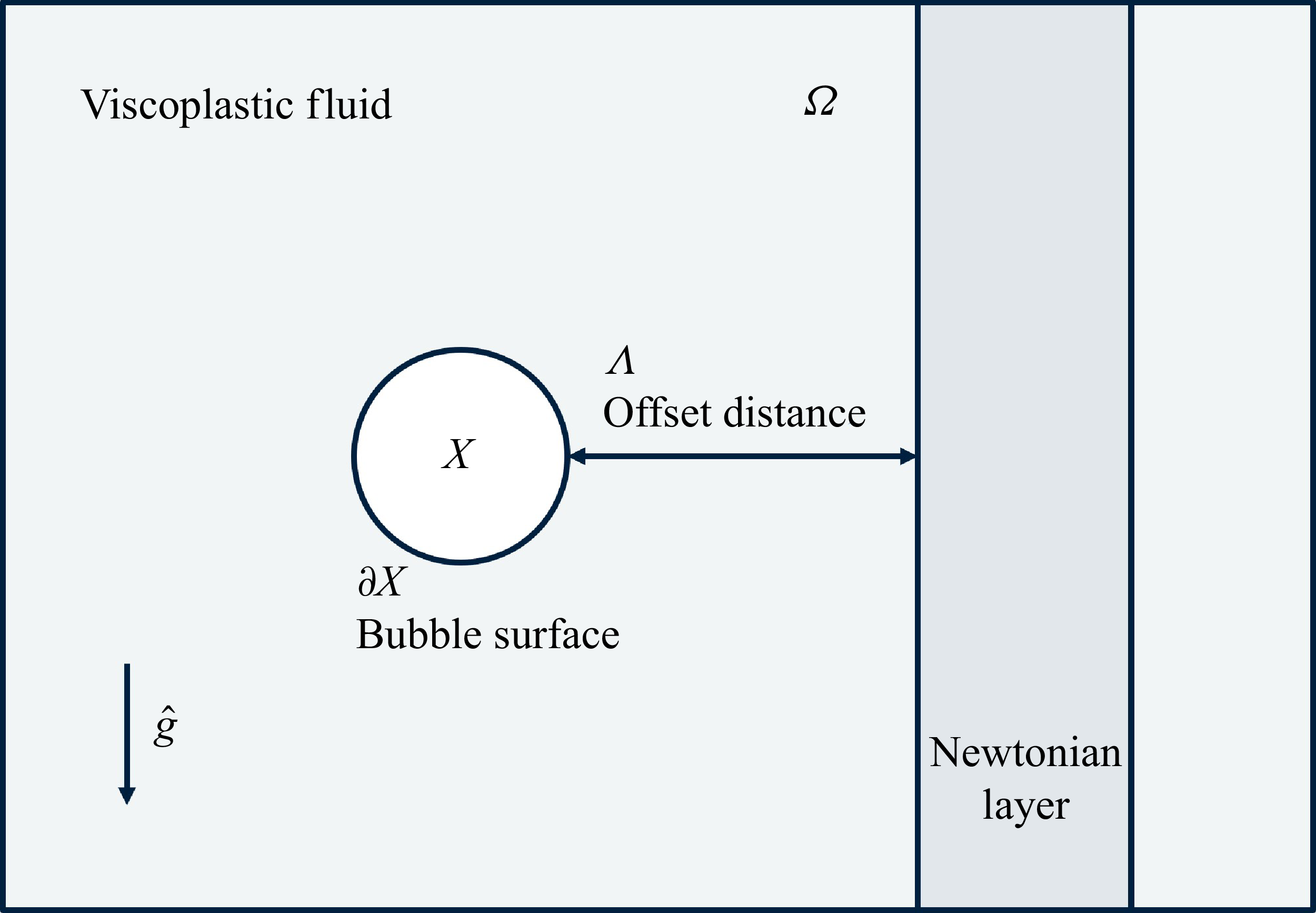
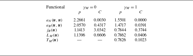
 f∼Cxp
f∼Cxp γM=0
γM=0 γM=1
γM=1
 Y→Yc−
Y→Yc− χ=0.5
χ=0.5 Λ=1
Λ=1 μ=0.001
 γM=0
γM=0 Yc=0.2197
 γM=1
γM=1 Yc=0.3829
 aN(u,u)
 aB(u,u)
 j(u)
j(u) LM(u)
LM(u) TM(u)
TM(u)
 (log‖γ˙‖)
 χ=0.5
χ=0.5 Λ=1
Λ=1 γM=0
γM=0 Y=0.13
 Y=0.16
 Y=0.19
 Y=0.22
 χ=0.5
χ=0.5 γM=1
γM=1 B=100
B=100 Y=0.277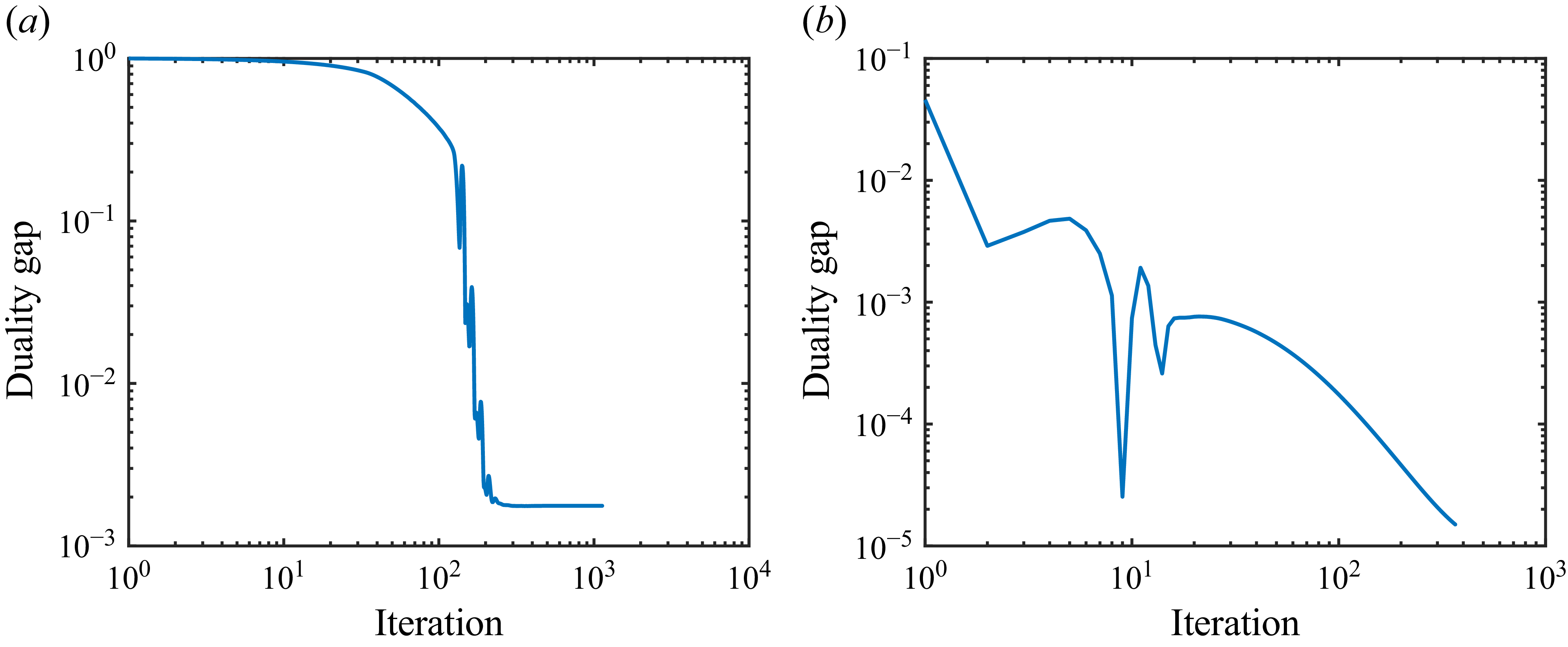
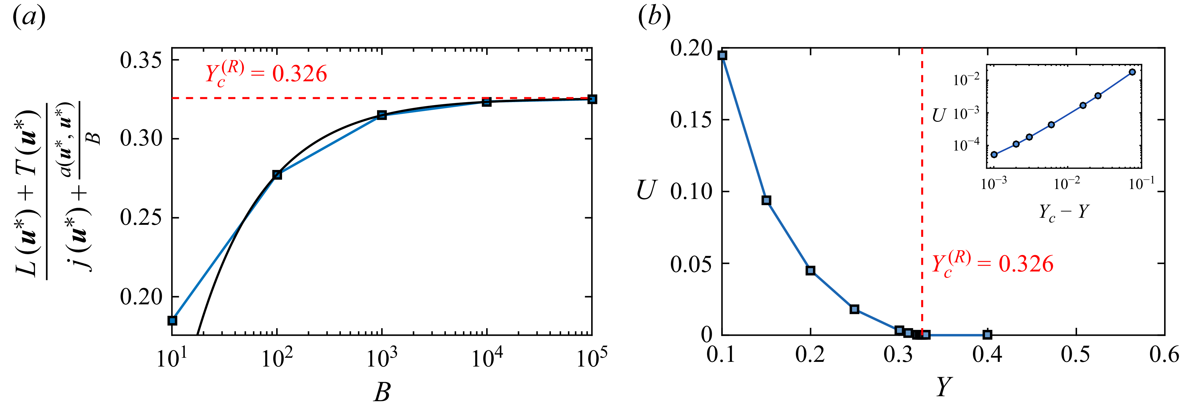
 Yc
Yc χ=0.5
χ=0.5 γM=1
γM=1 Y
Y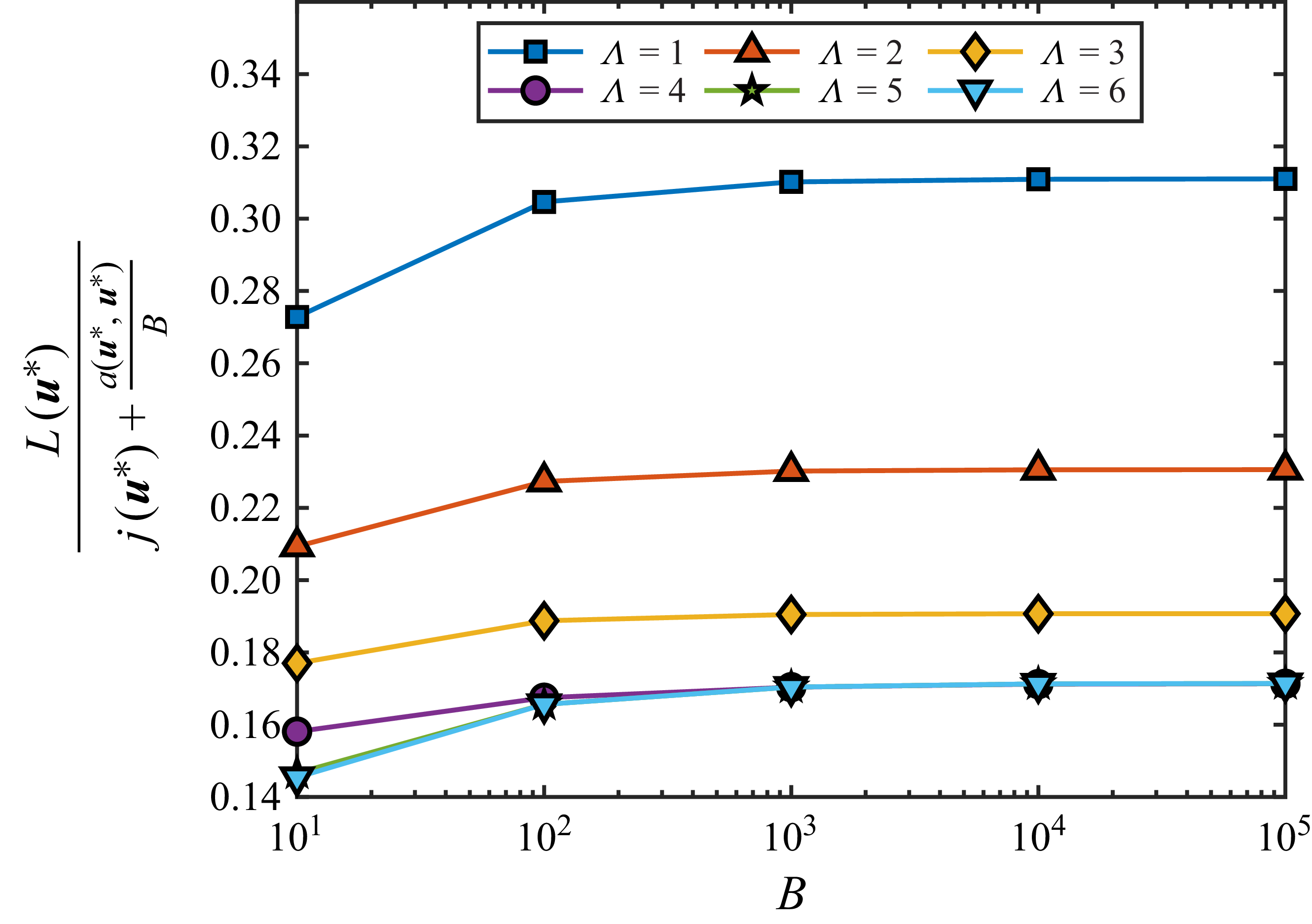
 Yc
Yc γM=0
γM=0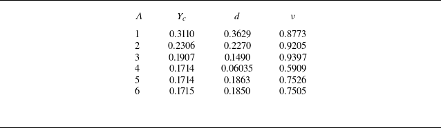
 Yc
Yc d
d ν
ν χ=1
χ=1
 log‖γ˙‖
 ||τ||
||τ|| B=10
B=10 B=1000
 Λ=3
Λ=3 γM=0
γM=0
 Yc
Yc χ=0.5
χ=0.5 χ=2
χ=2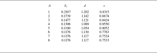
 Yc
Yc d
d ν
ν χ=0.5
χ=0.5 γM=0
γM=0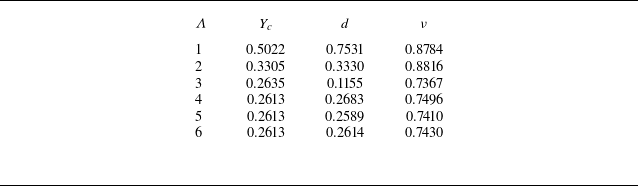
 Yc
Yc d
d ν
ν χ=2
χ=2 γM=0
γM=0
 Yc
Yc Λc
Λc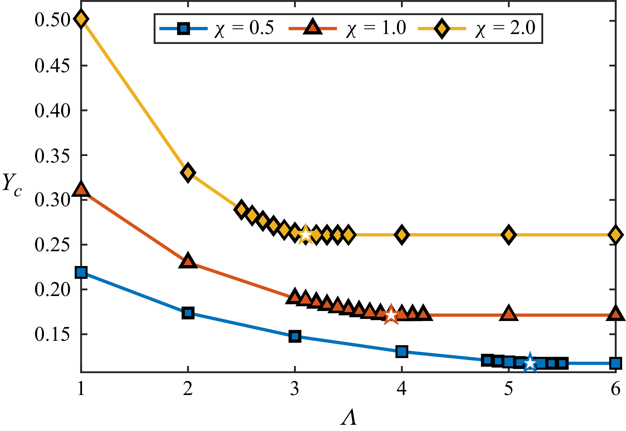
 Yc
Yc Yc∞
Yc∞ Λ
Λ χ
χ ⋆
⋆
 log‖γ˙‖
 ||τ||
||τ|| B=100
B=100 γM=0
γM=0 Λ=3
Λ=3 χ=0.5
χ=0.5 χ=2
χ=2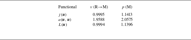
 j(u)
j(u) a(u,u)
 L(u)
L(u) →
→
 R→M
R→M M
M χ=0.5
χ=0.5 Λ=1
Λ=1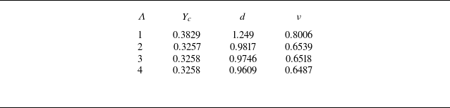
 Yc
Yc d
d ν
ν χ=0.5
χ=0.5 γM=1
γM=1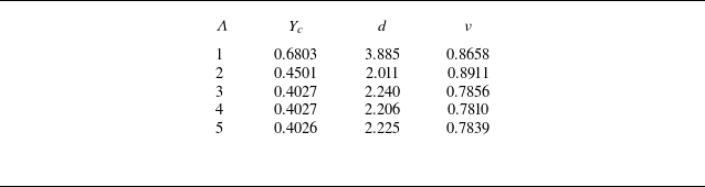
 Yc
Yc d
d ν
ν χ=2
χ=2 γM=1
γM=1
 Yc
Yc γM=1
γM=1 χ=0.5
χ=0.5 χ=2
χ=2
 log‖γ˙‖
 ||τ||
||τ|| B=10
B=10 γM=1
γM=1 Λ=3
Λ=3 χ=0.5
χ=0.5 χ=2
χ=2
 Yc
Yc μN/μP
μN/μP χ=1
χ=1 Λ=3
Λ=3 γM=0
γM=0 Yc
Yc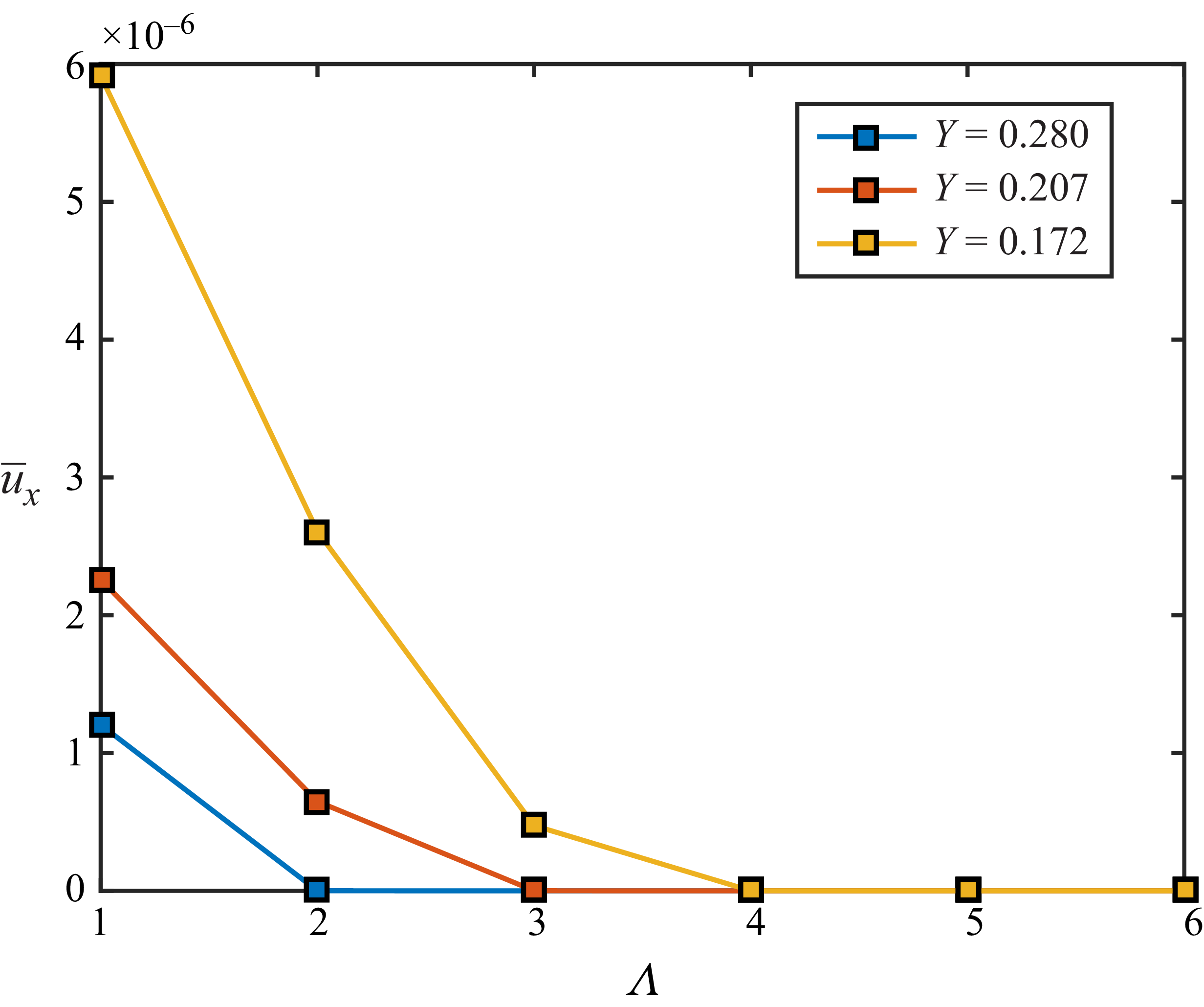
 u¯x
u¯x Λ
Λ Y
Y χ=1
χ=1 γM=0
γM=0
 Λ
Λ χ=0.5
χ=0.5 γM=1
γM=1 u¯x
u¯x u¯y
u¯y
 Λ
Λ χ=2
χ=2 γM=1
γM=1 u¯x
u¯x u¯y
u¯y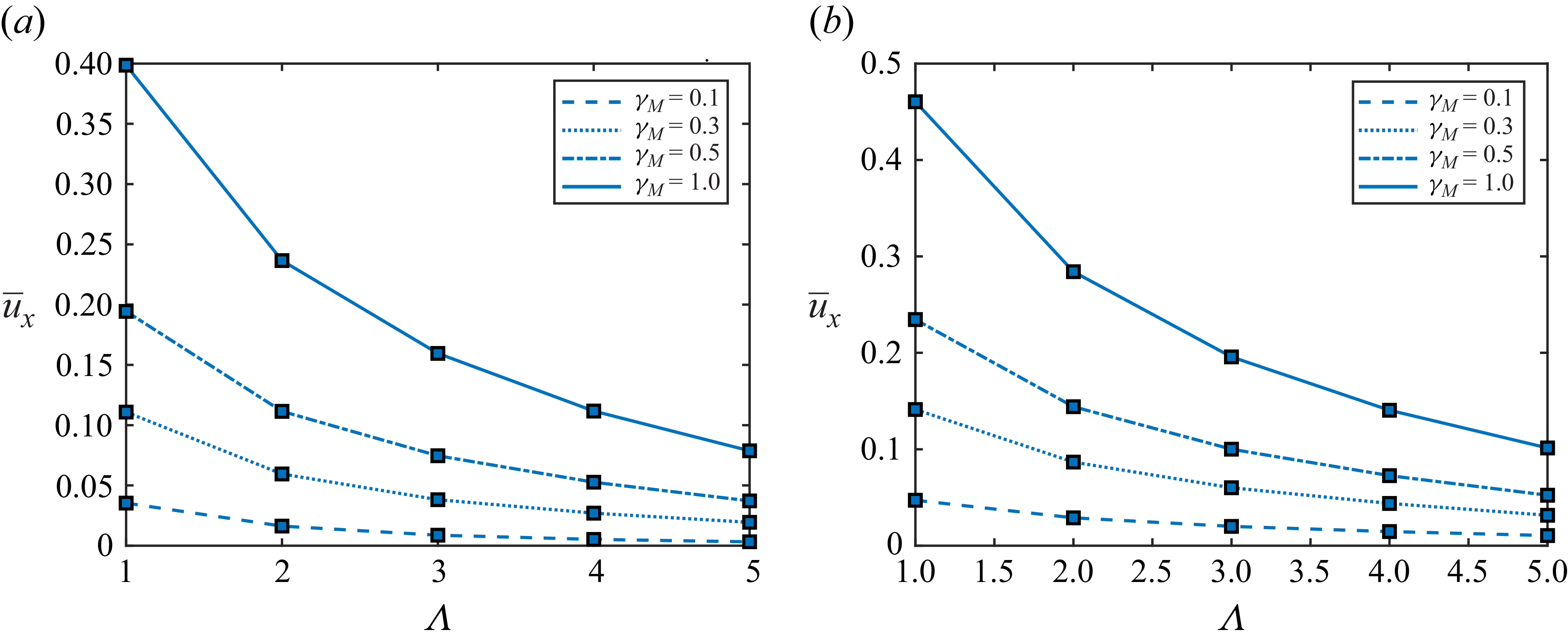
 Λ
Λ Y=0.05
 χ=0.5
χ=0.5 χ=2
χ=2
 Open access

