


1. Introduction
The topic of threshold crossing by a process has been extensively studied in probabilistic literature. When the process is a one-dimensional diffusion that solves a classical stochastic differential equation (SDE) with sufficiently regular coefficients, the number of crossings of a threshold $\zeta \in \mathbb{R}$
provides consistent estimations of the local time at
$\zeta \in \mathbb{R}$
provides consistent estimations of the local time at $\zeta $
(e.g. [Reference Azas6, Reference Jacod21, Reference Jacod22]; for a definition of local time see Section 2.1). Similar results have been developed for diffusions with a skew threshold or with discontinuous coefficients, allowing for estimation of localized features of a diffusion, such as the localized diffusion coefficient (e.g. [Reference Florens15]), the skew parameter [Reference Lejay, Mordecki and Torres26, Reference Mazzonetto27], and the oscillation jump of the diffusion coefficient [Reference Mazzonetto27]. Despite these advances, the limit behavior at a sticky threshold remains not well understood.
$\zeta $
(e.g. [Reference Azas6, Reference Jacod21, Reference Jacod22]; for a definition of local time see Section 2.1). Similar results have been developed for diffusions with a skew threshold or with discontinuous coefficients, allowing for estimation of localized features of a diffusion, such as the localized diffusion coefficient (e.g. [Reference Florens15]), the skew parameter [Reference Lejay, Mordecki and Torres26, Reference Mazzonetto27], and the oscillation jump of the diffusion coefficient [Reference Mazzonetto27]. Despite these advances, the limit behavior at a sticky threshold remains not well understood.
In this paper, we study the limit behavior of the number of the threshold 0 by time discretization of the sticky Brownian motion, as the discretization step vanishes. Sticky Brownian motion is a diffusion process that behaves like the standard Brownian motion away from 0 and spends a positive amount of time at 0 upon contact (see the definition in Section 2.2). The set of times at which the process is at 0 forms a totally disconnected random set of positive Lebesgue measure. This contrasts with the standard Brownian motion, whose zeroes form an uncountable, totally disconnected set, but of Lebesgue measure 0 (see, e.g., [Reference Revuz and Yor30, Proposition III.3.12]).
To the best of our knowledge, the only established result about number of crossings at the sticky threshold 0 by a sticky Brownian motion $(X_t)_{t\ge 0}$
is due to Gikhman. The result states that for every
$(X_t)_{t\ge 0}$
is due to Gikhman. The result states that for every $t\ge 0$
, as n goes to infinity, the statistic
$t\ge 0$
, as n goes to infinity, the statistic $\sum_{i=1}^{[nt]}\mathbf{1}_{\{{X}^{}_{({{i-1}})/{n}}{X}^{}_{{{i}}/{n}}<0\}}$
converges in law to some non-trivial discrete random variable (see [Reference Portenko29, §8], stated here in Theorem 2.1). This contrasts with the standard Brownian motion, where this statistic, renormalized by
$\sum_{i=1}^{[nt]}\mathbf{1}_{\{{X}^{}_{({{i-1}})/{n}}{X}^{}_{{{i}}/{n}}<0\}}$
converges in law to some non-trivial discrete random variable (see [Reference Portenko29, §8], stated here in Theorem 2.1). This contrasts with the standard Brownian motion, where this statistic, renormalized by $\sqrt{\pi/2n}$
, converges in probability to its local time at 0.
$\sqrt{\pi/2n}$
, converges in probability to its local time at 0.
In the case of sticky Brownian motion, we distinguish between three types of crossings and establish the limit behavior of each respective renormalized number-of-crossings statistic. Unlike Brownian motion, we show that the normalizing sequence depends on the type of crossing considered. One type of crossing provides a statistic whose renormalized limit matches the one observed in the Brownian case. Understanding the limit behavior of all these statistics is a crucial step before tackling the open question of the convergence rates to the local time at a sticky threshold. For non-sticky processes, these have been obtained in [Reference Jacod21, Theorem 1.2] for classical diffusions and [Reference Mazzonetto27] for skew threshold diffusions.
Ultimately, establishing such rates would enable us to obtain similar rates for the stickiness parameter estimators established here and in [Reference Anagnostakis3, Reference Anagnostakis and Mazzonetto5], which are built on such approximations. To highlight the importance of the estimation problem, let us mention a few applications of sticky diffusions. These processes are used in finance to model price dynamics on assets subject to takeover offers (see [Reference Criens and Urusov11]); in quantum mechanics, to model motions of particles near a source of emission (see [Reference Davies and Truman12]); in classical mechanics, to model motions of coarse particles in colloids (see [Reference Bou-Rabee and Holmes-Cerfon9] and references therein); and in epidemics, to model concentrations of pathogens in an organism (see [Reference Calsina and Farkas10]) – during an infection, these concentrations are random and significant, whereas off-infection, they keep close to zero.
Another contribution of this paper is the introduction of the symmetric counterpart of crossings, called bouncings, defined here as rebounds of the time discretization of the process at some threshold. As with crossings, we distinguish three kinds of bouncing and prove that the respective number of bouncings has the same asymptotic properties as the number of crossings of the same kind. We combine results on bouncings and crossings to establish results on sticky–reflected Brownian motion (see Section 5.1 for a definition), where only bouncing behavior is possible, and also on some sticky Itô diffusions. Our findings allow for the construction of a consistent stickiness parameter estimator, which we numerically show to converge at a comparable or faster rate than the existing estimators in [Reference Anagnostakis3, Reference Anagnostakis and Mazzonetto5].
The paper is organized as follows. In Section 2, we introduce sticky Brownian motion, along with several notions and results that are useful for this paper. In Section 3, we state the main results, namely, the limit behavior of the considered number-of-crossings and -bouncings statistics (Theorems 3.1 and 3.2) and the consistency of a stickiness parameter estimator based on these (Proposition 3.2). In Section 4, we prove these results. In Section 5, we extend the results to sticky–reflected Brownian motion and to smooth Itô diffusions with a sticky threshold. Section 6 is dedicated to numerical experiments on the stickiness parameter estimator devised here.
In the Appendix we prove several useful results. More precisely, in Appendix A, we prove asymptotic results on the sticky Brownian motion transition kernel, and in Appendix B, we prove a reflection principle at 0 for sticky Brownian motion.
2. Preliminary notions and results
In this section we state preliminary notions and results useful for the rest of the paper. We begin by defining the sticky Brownian motion, recall its probability transition kernel and its space–time scaling property. Then, we recall two notions of convergence. The first is convergence uniform in time, in probability, in which the local time approximation results are expressed and which retains the functional character of the approximation. The second is conditional convergence in probability, in which the estimation results are expressed. The estimators are indeed consistent only on the event that the threshold of interest (0 in our case) is hit by the process. Last, we state convergence results, in particular a local time approximation result previously established in [Reference Anagnostakis and Mazzonetto5], to which the proofs of our main results reduce.
2.1. Local time
We start by recalling the definition of the local time, which plays a fundamental role in our analysis. Indeed, in many cases, it will be the limiting process of our statistics of interest.
The local time of a semi-martingale, X, is the random field $(L^{a}_{t}(X);\, a\in \mathbb{R},\,t\ge 0) $
, defined for all
$(L^{a}_{t}(X);\, a\in \mathbb{R},\,t\ge 0) $
, defined for all $t\ge 0 $
,
$t\ge 0 $
, $a\in \mathbb{R}$
as the term
$a\in \mathbb{R}$
as the term $L^{a}_{t}(X)$
such that the following equation holds (see [Reference Revuz and Yor30, Theorem 1.2]):
$L^{a}_{t}(X)$
such that the following equation holds (see [Reference Revuz and Yor30, Theorem 1.2]):
 \begin{equation*} |X_t - a| = |X_0 - a| + \int_{0}^{t} \mathrm{sgn}(X_s - a) \,\mathrm{d} X_s + L^{a}_{t}(X).\end{equation*}
Here we used the convention $\mathrm{sgn}(x)=\mathbf{1}_{\{x>0\}}-\mathbf{1}_{\{x\le 0\}}$
.
$\mathrm{sgn}(x)=\mathbf{1}_{\{x>0\}}-\mathbf{1}_{\{x\le 0\}}$
.
For all $a\in\mathbb{R}$
,
$a\in\mathbb{R}$
, $t \mapsto L^{a}_{t}(X)$
is increasing and is fully supported on
$t \mapsto L^{a}_{t}(X)$
is increasing and is fully supported on $\{t\ge 0\colon X_t = a\} $
. This means that, for all
$\{t\ge 0\colon X_t = a\} $
. This means that, for all $t \ge 0$
,
$t \ge 0$
, $\int_{0}^{t}\mathbf{1}_{\{|X_s-a| \not = 0\}} \,\mathrm{d} L^{a}_{s}(X) = 0$
.
$\int_{0}^{t}\mathbf{1}_{\{|X_s-a| \not = 0\}} \,\mathrm{d} L^{a}_{s}(X) = 0$
.
The local time field can alternatively be defined as the following almost sure limit (see [Reference Revuz and Yor30, Corollary VI.1.9]):
 \begin{equation*} \text{for all}\ t\ge 0,\ a\in \mathbb{R},\ \text{almost surely}, \quad L^{a}_{t}(X) = \lim_{\varepsilon \rightarrow 0}\frac{1}{\varepsilon} \int_{0}^{t}\mathbf{1}_{\{X_s \in [a,a + \varepsilon)\}}\,\mathrm{d}\langle X\rangle_s.\end{equation*}
2.2. The sticky Brownian motion
We now provide a definition of sticky Brownian motion as a general linear diffusion on the real line described by scale function and speed measure. We explain the role of the stickiness parameter without discussing further what the scale function and speed measure are. Instead, we provide other equivalent characterizations of the process that are useful in the proofs of our results.
Sticky Brownian motion of stickiness parameter $\rho>0$
is the diffusion process on
$\rho>0$
is the diffusion process on $\mathbb{R}$
, on natural scale, with speed measure
$\mathbb{R}$
, on natural scale, with speed measure $m(\mathrm{d} x) = \mathrm{d}x + \rho\,\delta_{0}(\mathrm{d}x)$
(see, e.g., [Reference Borodin and Salminen8, pp. 123--124]). The parameter
$m(\mathrm{d} x) = \mathrm{d}x + \rho\,\delta_{0}(\mathrm{d}x)$
(see, e.g., [Reference Borodin and Salminen8, pp. 123--124]). The parameter $\rho>0$
, called the stickiness parameter, expresses the propensity of the process to stick at 0. The higher it is, the more time the process spends on average at 0. The asymptotic case
$\rho>0$
, called the stickiness parameter, expresses the propensity of the process to stick at 0. The higher it is, the more time the process spends on average at 0. The asymptotic case $\rho = 0$
corresponds to standard Brownian motion and
$\rho = 0$
corresponds to standard Brownian motion and $\rho=\infty$
to Brownian motion with an absorbing boundary at 0. In this paper we deal only with the case
$\rho=\infty$
to Brownian motion with an absorbing boundary at 0. In this paper we deal only with the case $\rho \in (0,\infty) $
. The Brownian motion case is known and the absorbing case is trivial.
$\rho \in (0,\infty) $
. The Brownian motion case is known and the absorbing case is trivial.
We now provide some useful equivalent characterizations of sticky Brownian motion. Let $\mathcal P_x = (\Omega, \mathcal{F}, (\mathcal{F}_t)_{t\ge 0}, \mathbb{P}_x)$
be a filtered probability space. The subscript x in
$\mathcal P_x = (\Omega, \mathcal{F}, (\mathcal{F}_t)_{t\ge 0}, \mathbb{P}_x)$
be a filtered probability space. The subscript x in $\mathcal P_x$
is a notational choice to indicate the starting point of the process. The filtrations
$\mathcal P_x$
is a notational choice to indicate the starting point of the process. The filtrations $(\mathcal F_t)_{t\ge 0}$
as well as all filtrations in this paper are assumed to satisfy the usual conditions (right-continuity and completeness).
$(\mathcal F_t)_{t\ge 0}$
as well as all filtrations in this paper are assumed to satisfy the usual conditions (right-continuity and completeness).
The following hold (see, e.g., [Reference Itô20, Sections 5.1, 5.2] and [Reference Rogers and Williams31, Theorem 47.1 and Remark (ii), p. 277]):
-
(t1) Let X be a sticky Brownian motion of stickiness parameter $\rho$
, defined on
$\mathcal P_x$
such that,
$\mathbb{P}_x$
-almost surely (a.s.),
$X_0=x$
. (In particular, X is
$(\mathcal{F}_t)_{t\ge 0}$
-adapted.) There exists a Brownian motion Z, defined on an extension of
$\mathcal P_x$
, such that
$X=(Z_{\gamma(t)})_{t\ge 0}$
, where the time change
$\gamma$
is the right-inverse of
$A(t) \;:\!=\; t + \rho L^{0}_{t}(Z_{})$
,
$t\ge 0$
, given by
$\gamma(t)\;:\!=\;\inf\{s>0 \colon A(s)>t\}$
and where
$L^{0}_{t}(Z_{})$
is the right local time at 0 of the process
$Z_{}$
.
$\rho$
, defined on
$\mathcal P_x$
such that,
$\mathbb{P}_x$
-almost surely (a.s.),
$X_0=x$
. (In particular, X is
$(\mathcal{F}_t)_{t\ge 0}$
-adapted.) There exists a Brownian motion Z, defined on an extension of
$\mathcal P_x$
, such that
$X=(Z_{\gamma(t)})_{t\ge 0}$
, where the time change
$\gamma$
is the right-inverse of
$A(t) \;:\!=\; t + \rho L^{0}_{t}(Z_{})$
,
$t\ge 0$
, given by
$\gamma(t)\;:\!=\;\inf\{s>0 \colon A(s)>t\}$
and where
$L^{0}_{t}(Z_{})$
is the right local time at 0 of the process
$Z_{}$
. -
(t2) Let Z be a standard Brownian motion, defined on the probability space
$\mathcal P_x$
, such that,
$\mathbb{P}_x$
-a.s.,
$Z_0=x$
. Then the process
$X \;:\!=\; (Z_{\gamma(t)})_{t\ge0}$
with
$\gamma$
defined in (t1) is a sticky Brownian motion of stickiness parameter
$\rho$
, and,
$\mathbb{P}_x$
-a.s.,
$X_0 = x $
.










Also, the following SDE characterization holds.
-
(p1) Let X be a sticky Brownian motion of stickiness parameter
$\rho$
, defined on the probability space
$\mathcal P_x$
, such that,
$\mathbb{P}_x$
-a.s.,
$X_0=x$
. There exists a Brownian motion W defined on an extension of
$\mathcal P_x $
such that (X, W) solves (2.1) -
(p2) The system (2.1) has a jointly unique weak solution [Reference Engelbert and Peskir13, Theorem 1] and it is a sticky Brownian motion of stickiness parameter
$\rho$
.


A proof of the last two statements for some sticky diffusions can be found in [Reference Anagnostakis3, Proposition 4.2] for (p1) and in [Reference Anagnostakis3, Theorem 4.1] for (p2). For sticky Brownian motion these proofs are contained in the proof of [Reference Engelbert and Peskir13, Theorem 1].
For an historical overview of sticky Brownian motion, see [Reference Peskir28]. For results on this process, see, e.g., [Reference Amir2, Reference Anagnostakis3, Reference Anagnostakis and Mazzonetto5, Reference Davies and Truman12, Reference Howitt19, Reference Salins and Spiliopoulos32]. For applications, see [Reference Bou-Rabee and Holmes-Cerfon9] and references therein.
Remark 2.1. (Occupation time and local time.) The second line of the system (2.1) states that the occupation time of the process at 0 is proportional to its local time at 0. This is related to the fact that the process spends a positive amount of time at the threshold 0.
2.3. Notions of convergence
The results on local time approximation are formulated in terms of the types of convergence introduced below. For convenience, let $(A_n)_{n\ge 0}$
be a sequence of real-valued processes defined on the probability space
$(A_n)_{n\ge 0}$
be a sequence of real-valued processes defined on the probability space $(\Omega, \mathcal F, \mathbb{P})$
.
$(\Omega, \mathcal F, \mathbb{P})$
.
Definition 2.1. We say that $(A^{n})_{n\ge1}$
converges locally uniformly in time, in probability to
$(A^{n})_{n\ge1}$
converges locally uniformly in time, in probability to $A^{0}$
if, for all
$A^{0}$
if, for all $t\ge 0$
,
$t\ge 0$
,

We denote this convergence with

The following result gives a sufficient condition for ucp convergence to occur.
Lemma 2.1. (cf. [Reference Jacod and Protter23, §2.2.3].) Assume that $A^n$
, for all
$A^n$
, for all $n\ge 1 $
, and
$n\ge 1 $
, and $A^{0}$
have increasing paths, and
$A^{0}$
have increasing paths, and $A^{0}$
is continuous. If there exists D dense in
$A^{0}$
is continuous. If there exists D dense in $[0,\infty)$
such that
$[0,\infty)$
such that $A^{n}_{t} \overset{\mathbb{P}}{\longrightarrow} A^{0}_t$
for all
$A^{n}_{t} \overset{\mathbb{P}}{\longrightarrow} A^{0}_t$
for all $t \in D$
, then
$t \in D$
, then  .
.
For the estimation result we adopt the notion of conditional convergence in probability. The reason is that the estimators we consider are consistent conditionally on the event that the threshold of interest (assumed located at 0) is reached. For an event $\mathcal H $
with
$\mathcal H $
with $\mathbb{P}(\mathcal H)\neq 0$
, let
$\mathbb{P}(\mathcal H)\neq 0$
, let $\mathbb{P}^{\mathcal H}(\!\cdot\!) \;:\!=\; \mathbb{P}(\cdot\mid \mathcal H)$
be the conditional probability on
$\mathbb{P}^{\mathcal H}(\!\cdot\!) \;:\!=\; \mathbb{P}(\cdot\mid \mathcal H)$
be the conditional probability on $\mathcal H $
.
$\mathcal H $
.
Definition 2.2. We say that the sequence of random variables $(X_{n})_{n\ge 1}$
converges to the random variable
$(X_{n})_{n\ge 1}$
converges to the random variable $X_{0}$
in probability, conditionally on the event
$X_{0}$
in probability, conditionally on the event $\mathcal H$
with positive probability, if
$\mathcal H$
with positive probability, if $X_{n} \longrightarrow X_{0}$
in
$X_{n} \longrightarrow X_{0}$
in $\mathbb{P}^{\mathcal H}$
-probability. We denote this convergence with
$\mathbb{P}^{\mathcal H}$
-probability. We denote this convergence with

2.4. Existing useful asymptotic results
For establishing the limit behavior of the number-of-crossings statistics we use the following existing results on sticky Brownian motion: an approximation of the local time, an approximation of the occupation time at 0, and a result on discrete martingales. We conclude the section by recalling a previously established limit in law of the number of crossings (of a precise type, type 0, described in Section 3), that we do not use in the paper because we have not found a proof.
Proposition 2.1. ([Reference Anagnostakis and Mazzonetto5, Proposition 6.3].) Let X be a sticky Brownian motion of stickiness parameter $\rho>0$
, defined on the filtered probability space
$\rho>0$
, defined on the filtered probability space $(\Omega, \mathcal{F}, (\mathcal{F}_t)_{t\ge 0},\mathbb{P}_x)$
, such that,
$(\Omega, \mathcal{F}, (\mathcal{F}_t)_{t\ge 0},\mathbb{P}_x)$
, such that, $\mathbb{P}_x$
-a.s.,
$\mathbb{P}_x$
-a.s., $X_0=x$
. Let
$X_0=x$
. Let $m_{\sqrt n \rho}$
be the measure defined for all
$m_{\sqrt n \rho}$
be the measure defined for all $x\in \mathbb{R}$
by
$x\in \mathbb{R}$
by
 \begin{equation} m_{\sqrt n \rho}(\mathrm{d}x) = \mathrm{d}x + \sqrt n\rho\,\delta_{0}(\mathrm{d}x) \end{equation}
and $(g_{n})_{n}$
a sequence of measurable real functions such that, for all
$(g_{n})_{n}$
a sequence of measurable real functions such that, for all $x\in \mathbb{R}$
,
$x\in \mathbb{R}$
,
 \begin{align} &\lim_{n \longrightarrow \infty}\bigg(\frac{g_{n}^2(\sqrt n x)}{n} + \frac{m_{\sqrt n \rho}(g^{2}_n)}{\sqrt n}\nonumber \\ &\quad + \frac{\big(\int_{-\infty}^{+\infty}|x|g_n(x)\,\mathrm{d}x\big)(1 + \log(n))g_n(\sqrt n x)}{n} + \frac{{(1 + \log(n))m_{\sqrt n \rho}(|g_n|)}}{\sqrt n}\bigg) = 0 \end{align}
and $\lim_{n\to \infty}m_{\sqrt n \rho}(g_n) = M$
. Then, for all
$\lim_{n\to \infty}m_{\sqrt n \rho}(g_n) = M$
. Then, for all $t \geq 0$
,
$t \geq 0$
,

Also, if (2.3) holds and $\sup_n\big(m_{\sqrt n \rho}(|g_n|)\big) < \infty$
then the above convergence is localy uniform in time, in
$\sup_n\big(m_{\sqrt n \rho}(|g_n|)\big) < \infty$
then the above convergence is localy uniform in time, in $\mathbb{P}_x$
-probability.
$\mathbb{P}_x$
-probability.
In Proposition 2.1, as well as throughout the paper, we use the notation
 \begin{equation} m_{\sqrt n \rho}(g) = \int_{\mathbb{R}}g(x)\,m_{\sqrt n \rho}(\mathrm{d} x) = \int_{-\infty}^{+\infty}g(x)\,\mathrm{d}x + \sqrt{n}\rho g(0)\end{equation}
for any integrable function g.
Lemma 2.2. ([Reference Anagnostakis and Mazzonetto5, Lemma 3.7].) Let X be a sticky Brownian motion of stickiness parameter $\rho>0$
, defined on the filtered probability space
$\rho>0$
, defined on the filtered probability space $(\Omega,\mathcal{F},(\mathcal{F}_t)_{t\ge 0},\mathbb{P}_x)$
such that,
$(\Omega,\mathcal{F},(\mathcal{F}_t)_{t\ge 0},\mathbb{P}_x)$
such that, $\mathbb{P}_x$
-a.s.,
$\mathbb{P}_x$
-a.s., $X_0=x$
. Then, for all intervals U (including singletons),
$X_0=x$
. Then, for all intervals U (including singletons),
 \begin{equation*} \frac{1}{n}\sum_{i=1}^{[n\cdot]}\mathbf{1}_{\{{X}_{({{i-1}})/{n}} \in U\}} \xrightarrow[n \longrightarrow \infty]{\mathbb{P}_x\text{-}\mathrm{ucp}} \int_{0}^{\cdot}\mathbf{1}_{\{X_s \in U\}}\,\mathrm{d}s. \end{equation*}
In particular, taking $U=\{0\}$
,
$U=\{0\}$
,
 \begin{equation*} \frac{1}{n}\sum_{i=1}^{[n\cdot]}\mathbf{1}_{\{{X}_{({{i-1}})/{n}} = 0\}} \xrightarrow[n \longrightarrow \infty]{\mathbb{P}_x\text{-}\mathrm{ucp}} \int_{0}^{\cdot}\mathbf{1}_{\{X_s = 0\}}\,\mathrm{d}s = \rho L^{0}_{}(X). \end{equation*}
See also [Reference Altmeyer1] for the approximation of smooth occupation time functionals.
Lemma 2.3. ([Reference Genon-Catalot and Jacod17, Lemma 9].) Let $\mathcal P = (\Omega,\mathcal{F},\mathbb{P})$
be a probability space,
$\mathcal P = (\Omega,\mathcal{F},\mathbb{P})$
be a probability space, $((\mathcal{F}^{n}_{i})_{i})_n$
a family of discrete filtrations on
$((\mathcal{F}^{n}_{i})_{i})_n$
a family of discrete filtrations on $\mathcal P$
,
$\mathcal P$
, $(\chi^{n}_i)_{i,n}$
a family of random variables on
$(\chi^{n}_i)_{i,n}$
a family of random variables on $\mathcal P$
such that, for all (i, n),
$\mathcal P$
such that, for all (i, n), $\chi^{n}_i$
is
$\chi^{n}_i$
is $\mathcal{F}^{n}_{i}$
-measurable, and U a random variable on
$\mathcal{F}^{n}_{i}$
-measurable, and U a random variable on $\mathcal P$
. The following two conditions imply that
$\mathcal P$
. The following two conditions imply that 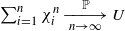 :
:
-
(i)
; -
(ii)
.
 ;
; .
.
Theorem 2.1. (Efimenko–Portenko (1989); see [Reference Portenko29].) We consider the setting of Lemma 2.2. For all $t>0$
,
$t>0$
, $\sum_{i=1}^{[nt]}\mathbf{1}_{\{{X}_{({{i-1}})/{n}}{X}_{{{i}}/{n}}<0\}}$
converges in law to some discrete random variable
$\sum_{i=1}^{[nt]}\mathbf{1}_{\{{X}_{({{i-1}})/{n}}{X}_{{{i}}/{n}}<0\}}$
converges in law to some discrete random variable $Z_t$
with values in
$Z_t$
with values in $\mathbb{N}_0 $
, i.e. there exists
$\mathbb{N}_0 $
, i.e. there exists $(b_k(t);\,k\in\mathbb{N}_0,\,t\ge 0)$
such that
$(b_k(t);\,k\in\mathbb{N}_0,\,t\ge 0)$
such that $\mathbb{P}_0(Z_t = k) = b_k(t)$
for all
$\mathbb{P}_0(Z_t = k) = b_k(t)$
for all $k\in\mathbb{N}_0$
. The probabilities
$k\in\mathbb{N}_0$
. The probabilities $(b_k(t);\, k\in\mathbb{N}_0,\,t\ge 0)$
are defined via their Laplace transforms
$(b_k(t);\, k\in\mathbb{N}_0,\,t\ge 0)$
are defined via their Laplace transforms
 \begin{equation*} \int_{0}^{\infty}\lambda{\mathrm{e}}^{-\lambda t}b_k(t)\,\mathrm{d}t = \frac{A_{\lambda}}{1/\rho^{2} + A_{\lambda}}\bigg(\frac{1/\rho^{2}}{1/\rho^{2}+A_{\lambda}}\bigg)^{k} \quad {for\ all}\ k\in\mathbb{N}_0\ { and\ all }\ t\ge 0, \end{equation*}
with $A_{\lambda} = \sqrt{\lambda}(\sqrt\lambda + \sqrt{2}/\rho)$
.
$A_{\lambda} = \sqrt{\lambda}(\sqrt\lambda + \sqrt{2}/\rho)$
.
3. Main results
We consider three types of behavior on the time interval $[t,t+s]$
of the process X at the sticky threshold. For simplicity, we assume the threshold to be located at 0.
$[t,t+s]$
of the process X at the sticky threshold. For simplicity, we assume the threshold to be located at 0.
The types of crossings are:
-
Type 0: The process crosses from one open half-plane to the other. For example if
$X_t <0 $
and
$X_{t+s}>0 $
. -
Type 1: The process crosses from one open or closed half-plane to its complementary. For example if
$X_t \le0 $
and
$X_{t+s}>0 $
, or if
$X_t <0 $
and
$X_{t+s} \ge 0 $
. -
Type 2: The process crosses from one closed half-plane to the other. For example
$X_t \le 0$
and
$X_{t+s}\ge 0$
.


The types of bouncings are:
-
Type 0: The process bounces from
$(0,\infty)$
back into
$(0,\infty)$
after hitting 0. For example if
$X_t >0$
,
$X_{t+s}>0$
, and, for some
$h\in[0,s]$
,
$X_{t+h}=0$
. -
Type 1: The process bounces from the closed half-plane to the open one or vice versa. For example if
$X_t > 0$
and
$X_{t+s}\ge 0$
, or if
$X_t >0$
and
$X_{t+s} \ge 0$
, and, for some
$h\in[0,s]$
,
$X_{t+h}=0$
. -
Type 2: The process bounces from
$[0,\infty)$
to
$[0,\infty)$
. For example
$X_t \ge 0 $
,
$X_{t+s}\ge 0 $
, and, for some
$u\in[t,t+s]$
,
$X_{u}=0$
.


We now define the crossing statistics based on discrete observations of the process. Assume we are given uniformly spaced in time observations of a process X over the interval [0, t], taken at times $i/n$
,
$i/n$
, $i = 0, 1, \dots, [nt]$
. That is, we are given
$i = 0, 1, \dots, [nt]$
. That is, we are given $(X_{i/n})_{i\le [nt]}$
.
$(X_{i/n})_{i\le [nt]}$
.
For $j\in \{0,1,2\}$
, the number-of-crossings statistic of type j is the number of times the time discretization
$j\in \{0,1,2\}$
, the number-of-crossings statistic of type j is the number of times the time discretization $(X_{i/n})_{i\le [nt]}$
of the process executes a crossing of type j at 0. In particular, for all
$(X_{i/n})_{i\le [nt]}$
of the process executes a crossing of type j at 0. In particular, for all $t \in (0,\infty)$
and
$t \in (0,\infty)$
and $n\in \mathbb{N} $
,
$n\in \mathbb{N} $
,
 \begin{align*} C^{(0)}_{n,t}(X) & \;:\!=\; \textstyle\sum_{i=1}^{[nt]}\mathbf{1}_{\{{X}_{({{i-1}})/{n}}{X}_{{{i}}/{n}}<0\}}, \\ C^{(1)}_{n,t}(X) & \;:\!=\; \textstyle\sum_{i=1}^{[nt]}\big(\mathbf{1}_{\{{X}_{({{i-1}})/{n}}{X}_{{{i}}/{n}}\le 0\}} - \mathbf{1}_{\{{X}_{({{i-1}})/{n}}={X}_{{{i}}/{n}} = 0\}}\big), \\ C^{(2)}_{n,t}(X) & \;:\!=\; \textstyle\sum_{i=1}^{[nt]}\mathbf{1}_{\{{X}_{({{i-1}})/{n}}{X}_{{{i}}/{n}}\le 0\}}.\end{align*}
Similarly, for all $t \in (0,\infty)$
and
$t \in (0,\infty)$
and $n\in \mathbb{N} $
, we define the number-of-bouncings statistics as
$n\in \mathbb{N} $
, we define the number-of-bouncings statistics as
 \begin{align*} B^{(0)}_{n,t}(X) & \;:\!=\; \textstyle\sum_{i=1}^{[nt]}\mathbf{1}_{U^{n}_{i}(X)}\mathbf{1}_{\{{X}_{({{i-1}})/{n}}{X}_{{{i}}/{n}}>0\}}, \\ B^{(1)}_{n,t}(X) & \;:\!=\; \textstyle\sum_{i=1}^{[nt]}\mathbf{1}_{U^{n}_{i}(X)}\big(\mathbf{1}_{\{{X}_{({{i-1}})/{n}}{X}_{{{i}}/{n}}\ge 0\}} - \mathbf{1}_{\{{X}_{({{i-1}})/{n}}={X}_{{{i}}/{n}} = 0\}}\big), \\ B^{(2)}_{n,t}(X) & \;:\!=\; \textstyle\sum_{i=1}^{[nt]}\mathbf{1}_{U^{n}_{i}(X)}\mathbf{1}_{\{{X}_{({{i-1}})/{n}}{X}_{{{i}}/{n}}\ge 0\}},\end{align*}
where, for all n, i, $U^{n}_{i}(X)$
is the event defined as
$U^{n}_{i}(X)$
is the event defined as
 \begin{equation*} U^{n}_{i}(X) = \{\text{there exists}\ s \in [{i-1}/{n},{i}/{n}]\ \text{such that}\ X_s = 0\}.\end{equation*}
We note that these statistics are different when the process spends a positive amount of time at 0 with positive probability. Indeed, if we define the difference statistics as
 \begin{equation*} \begin{aligned} \mathbf{Z}^{(1)}_{n,t}(X) \;:\!=\; C^{(1)}_{n,t}(X) - C^{(0)}_{n,t}(X) & = B^{(1)}_{n,t}(X) - B^{(0)}_{n,t}(X) \\ & = \sum_{i=1}^{[nt]}\mathbf{1}_{\{{X}_{({{i-1}})/{n}}=0;\,{X}_{{{i}}/{n}}\not= 0\}} + \sum_{i=1}^{[nt]}\mathbf{1}_{\{{X}_{({{i-1}})/{n}}\not = 0;\,{X}_{{{i}}/{n}}= 0\}}, \\ \mathbf{Z}^{(2)}_{n,t}(X) \;:\!=\; C^{(2)}_{n,t}(X) - C^{(1)}_{n,t}(X) & = B^{(2)}_{n,t}(X) - B^{(1)}_{n,t}(X) = \sum_{i=1}^{[nt]}\mathbf{1}_{\{{X}_{({{i-1}})/{n}}={X}_{{{i}}/{n}}= 0\}}, \end{aligned}\end{equation*}
then, for all t, n and $i=1,2$
, for sticky Brownian motion X we have
$i=1,2$
, for sticky Brownian motion X we have $\mathbf{Z}^{(i)}_{n,t}(X)>0 $
with positive probability. If X is a Brownian motion, then
$\mathbf{Z}^{(i)}_{n,t}(X)>0 $
with positive probability. If X is a Brownian motion, then $\mathbf{Z}^{(i)}_{n,t}(X)=0$
almost surely.
$\mathbf{Z}^{(i)}_{n,t}(X)=0$
almost surely.
It can be said that the $B^{(\,j)}$
are not statistics, since they depend on the events
$B^{(\,j)}$
are not statistics, since they depend on the events $(U_{n,i})_{n,i}$
that are not in the
$(U_{n,i})_{n,i}$
that are not in the $\sigma$
-algebra generated by high-frequency samples of the process. However, they are related to the difference statistics
$\sigma$
-algebra generated by high-frequency samples of the process. However, they are related to the difference statistics $\mathbf{Z}^{(1)}_{}$
,
$\mathbf{Z}^{(1)}_{}$
, $\mathbf{Z}^{(2)}_{} $
.
$\mathbf{Z}^{(2)}_{} $
.
3.1. Limit behavior of the statistics
The main result of this paper is the following.
Theorem 3.1. Let X be a sticky Brownian motion of stickiness parameter $\rho>0$
defined on the filtered probability space
$\rho>0$
defined on the filtered probability space $(\Omega, \mathcal{F}, (\mathcal{F}_t)_{t\ge 0},\mathbb{P}_x)$
such that,
$(\Omega, \mathcal{F}, (\mathcal{F}_t)_{t\ge 0},\mathbb{P}_x)$
such that, $\mathbb{P}_x$
-a.s.,
$\mathbb{P}_x$
-a.s., $X_0 = x$
(in particular, X is
$X_0 = x$
(in particular, X is $(\mathcal{F}_t)_{t\ge 0}$
-adapted), and let
$(\mathcal{F}_t)_{t\ge 0}$
-adapted), and let $L^{0}_{}(X)$
be the right local time at 0 of X. Then the following convergences hold:
$L^{0}_{}(X)$
be the right local time at 0 of X. Then the following convergences hold:
-
(i) for every diverging sequence
$u_n$
, ; -
(ii)
and ; -
(iii)
and ,

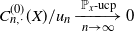 ;
; and
and  ;
; and
and  ,
, where, as per (2.1), $\rho L^{0}_{t}(X) = \int_{0}^{t}\mathbf{1}_{\{X_s = 0\}}\,\mathrm{d}s$
for all
$\rho L^{0}_{t}(X) = \int_{0}^{t}\mathbf{1}_{\{X_s = 0\}}\,\mathrm{d}s$
for all $t\ge 0$
.
$t\ge 0$
.
We note that in the case of the standard Brownian motion W, all three statistics have the same non-trivial limit for the same normalizing sequence $\sqrt{n}$
. Indeed, from, e.g., [Reference Jacod21, Theorem 1.1],
$\sqrt{n}$
. Indeed, from, e.g., [Reference Jacod21, Theorem 1.1],
 \begin{equation*} \mathop{\mathbb{P}{\kern.5pt}\text{-}{\kern.5pt}\text{lim}}\limits_{n\longrightarrow\infty}\bigg(\frac{C^{(0)}_{n,t}(W)}{\sqrt n}\bigg) = \mathop{\mathbb{P}{\kern.5pt}\text{-}{\kern.5pt}\text{lim}}\limits_{n\longrightarrow\infty}\bigg(\frac{C^{(1)}_{n,t}(W)}{\sqrt n}\bigg) = \mathop{\mathbb{P}{\kern.5pt}\text{-}{\kern.5pt}\text{lim}}\limits_{n\longrightarrow\infty}\bigg(\frac{C^{(2)}_{n,t}(W)}{\sqrt n}\bigg) = \sqrt{\frac{2}{\pi}} L^{0}_{t}(W).\end{equation*}
Also, the rates of convergence are known. In [Reference Jacod21, Theorem 1.2], a central limit theorem is proven for this convergence, with a rate of $n^{1/4}$
.
$n^{1/4}$
.
Unlike the standard Brownian motion, we observe that there is a factor 4 in the limits of $C^{(1)}_{n\cdot}/\sqrt n$
and
$C^{(1)}_{n\cdot}/\sqrt n$
and $\mathbf{Z}^{(1)}_{n,\cdot}/\sqrt n $
for sticky Brownian motion (see Theorem 3.1(ii)). This factor comes from the fact that
$\mathbf{Z}^{(1)}_{n,\cdot}/\sqrt n $
for sticky Brownian motion (see Theorem 3.1(ii)). This factor comes from the fact that $\mathbf{Z}^{(1)}_{n,t}/\sqrt n$
rewrites as a sum of four different terms, all converging to
$\mathbf{Z}^{(1)}_{n,t}/\sqrt n$
rewrites as a sum of four different terms, all converging to $\sqrt{2/\pi} L^{0}_{t}(X)$
. Indeed,
$\sqrt{2/\pi} L^{0}_{t}(X)$
. Indeed,
 \begin{equation*} \begin{aligned} \frac{1}{\sqrt{n}\,}\mathbf{Z}^{(1)}_{n,t}(X) & = \frac{1}{\sqrt{n}\,}\sum_{i=1}^{[nt]}\mathbf{1}_{\{{X}_{({{i-1}})/{n}}=0;\,{X}_{{{i}}/{n}}> 0\}} + \frac{1}{\sqrt{n}\,}\sum_{i=1}^{[nt]}\mathbf{1}_{\{{X}_{({{i-1}})/{n}}=0;\,{X}_{{{i}}/{n}} < 0\}} \\ & \quad + \frac{1}{\sqrt{n}\,}\sum_{i=1}^{[nt]}\mathbf{1}_{\{{X}_{({{i-1}})/{n}} > 0;\,{X}_{{{i}}/{n}}= 0\}} + \frac{1}{\sqrt{n}\,}\sum_{i=1}^{[nt]}\mathbf{1}_{\{{X}_{({{i-1}})/{n}} < 0;\,{X}_{{{i}}/{n}}= 0\}} . \end{aligned}\end{equation*}
Each term converges to 0 if the process is a standard Brownian motion W. For the sticky Brownian motion, the limit is instead non-trivial and it corresponds to the case of the renormalized number-of-crossings statistic for Brownian motion: $C^{(0)}_{n,\cdot}(W)/\sqrt n$
.
$C^{(0)}_{n,\cdot}(W)/\sqrt n$
.
Regarding the bouncing statistics, we prove the following.
Theorem 3.2. Consider the setting of Theorem 3.1. Then:
-
(i) For every diverging sequence
$u_n$
,
$B^{(0)}_{n,\cdot}/u_n$
has the same limit as
$C^{(0)}_{n,\cdot}(X) /u_n$
. -
(ii)
$B^{(\,j)}_{n,\cdot}/n^{\,j/2}$
has the same limit as
$C^{(\,j)}_{n,\cdot}(X) /n^{\,j/2}$
for
$j=1,2$
.


The difference statistics $\mathbf{Z}^{(\cdot)}_{}$
are the leading parts of number-of-crossings and -bouncings statistics of type 1 and 2.
$\mathbf{Z}^{(\cdot)}_{}$
are the leading parts of number-of-crossings and -bouncings statistics of type 1 and 2.
The proof of the above results relies, by virtue of Lemma 2.3, on the following limit behavior of the conditional version of the statistics $C^{(0)}_{}$
,
$C^{(0)}_{}$
, $C^{(1)}_{}$
, and
$C^{(1)}_{}$
, and $C^{(2)}_{}$
. These are the statistics
$C^{(2)}_{}$
. These are the statistics $\widetilde C^{(0)}_{}$
,
$\widetilde C^{(0)}_{}$
, $\widetilde C^{(1)}_{}$
, and
$\widetilde C^{(1)}_{}$
, and $\widetilde C^{(2)}_{}$
defined for all n, t as
$\widetilde C^{(2)}_{}$
defined for all n, t as
 \begin{align*} \widetilde C^{(0)}_{n,t}(X) & \;:\!=\; \textstyle\sum_{i=1}^{[nt]}\mathbb{E}_x\big(\mathbf{1}_{\{{X}_{({{i-1}})/{n}}{X}_{{{i}}/{n}}<0\}} \mid \mathcal{F}_{({i-1})/{n}}\big), \\ \widetilde C^{(1)}_{n,t}(X) & \;:\!=\; \textstyle\sum_{i=1}^{[nt]}\mathbb{E}_x\big(\mathbf{1}_{\{{X}_{({{i-1}})/{n}}{X}_{{{i}}/{n}}\le 0\}} - \mathbf{1}_{\{{X}_{({{i-1}})/{n}}={X}_{{{i}}/{n}} = 0\}} \mid \mathcal{F}_{({i-1})/{n}}\big), \\ \widetilde C^{(2)}_{n,t}(X) & \;:\!=\; \textstyle\sum_{i=1}^{[nt]}\mathbb{E}_x\big(\mathbf{1}_{\{{X}_{({{i-1}})/{n}}{X}_{{{i}}/{n}}\le 0\}} \mid \mathcal{F}_{({i-1})/{n}}\big).\end{align*}
For these, the following result holds.
Proposition 3.1. Consider the setting of Theorem 3.1. Then:
-
(i)
. -
(ii)
$\widetilde C^{(\,j)}_{n,\cdot}(X)/n^{\,j/2}$
has the same limit as
$C^{(\,j)}_{n,\cdot}(X)/n^{\,j/2}$
for
$j=1,2$
.
 .
.


The proof of Theorem 3.1(i) is done by bounding the distance between $ \widetilde C^{(0)}_{}$
and
$ \widetilde C^{(0)}_{}$
and $C^{(0)}_{} $
, and showing that both the distance and the limit of
$C^{(0)}_{} $
, and showing that both the distance and the limit of $\widetilde C^{(0)}_{}(X)$
, if renormalized by
$\widetilde C^{(0)}_{}(X)$
, if renormalized by $1/u_n $
, vanish in probability as
$1/u_n $
, vanish in probability as $n \longrightarrow \infty$
.
$n \longrightarrow \infty$
.
Let us note that the only case, for which the limits of the expected and non-expected versions of the number-of-crossings statistics are not necessarily the same is for the type 0 crossings (strict crossings). In fact, they cannot be the same since $C^{(0)}_{n,t}(X)$
and its limit take values in
$C^{(0)}_{n,t}(X)$
and its limit take values in $\mathbb{N} \cup (+\infty)$
, while the law of
$\mathbb{N} \cup (+\infty)$
, while the law of $(1/\rho) L^{0}_{t}(X) $
, the limit of
$(1/\rho) L^{0}_{t}(X) $
, the limit of $\widetilde C^{(0)}_{n,t}(X) $
, is continuous. The discrete limit law of
$\widetilde C^{(0)}_{n,t}(X) $
, is continuous. The discrete limit law of $C^{(0)}_{n,t}(X)$
is described in [Reference Portenko29, §8], which is restated here in Theorem 2.1. We also mention that Theorem 3.1(i) can also be inferred directly from Theorem 2.1.
$C^{(0)}_{n,t}(X)$
is described in [Reference Portenko29, §8], which is restated here in Theorem 2.1. We also mention that Theorem 3.1(i) can also be inferred directly from Theorem 2.1.
3.2. Estimation
In [Reference Anagnostakis3, Reference Anagnostakis and Mazzonetto5] an estimator was proposed based on a test function g and a normalizing sequence $u_n$
. More precisely, let g be a bounded integrable function that satisfies
$u_n$
. More precisely, let g be a bounded integrable function that satisfies $g(0)=0$
,
$g(0)=0$
, $(u_n)_n$
a sequence such that, as
$(u_n)_n$
a sequence such that, as $n \longrightarrow \infty$
,
$n \longrightarrow \infty$
, $u_n \longrightarrow \infty$
and
$u_n \longrightarrow \infty$
and $u_n/n \longrightarrow 0$
,
$u_n/n \longrightarrow 0$
, $\mathcal H_t$
be the event
$\mathcal H_t$
be the event $\big\{\tau^{X}_0<t\big\} = \{\text{there exists}\ s < t\ \text{such that}\ X_s = 0\}$
, and
$\big\{\tau^{X}_0<t\big\} = \{\text{there exists}\ s < t\ \text{such that}\ X_s = 0\}$
, and $\varrho^{(0)}_{n}(X)$
the statistic
$\varrho^{(0)}_{n}(X)$
the statistic
 \begin{equation} \varrho^{(0)}_{n}(X) \;:\!=\; \bigg(\int_{\mathbb{R}}g\,\mathrm{d}x\bigg)\frac{1}{u_n} \frac{\sum_{i=1}^{[nt]}\mathbf{1}_{\{{X}_{({{i-1}})/{n}}=0\}}}{\sum_{i=1}^{[nt]}g(u_n{X}_{({{i-1}})/{n}})}.\end{equation}
Then $\varrho^{(0)}_{n}(X) $
is a consistent estimator of
$\varrho^{(0)}_{n}(X) $
is a consistent estimator of $\rho $
conditionally on the event
$\rho $
conditionally on the event $\mathcal H_t $
, i.e.
$\mathcal H_t $
, i.e. $\varrho^{(0)}_{n}(X) \longrightarrow \rho $
in
$\varrho^{(0)}_{n}(X) \longrightarrow \rho $
in $\mathbb{P}^{\mathcal H_t}_x $
-probability as
$\mathbb{P}^{\mathcal H_t}_x $
-probability as $n \longrightarrow \infty $
.
$n \longrightarrow \infty $
.
We now devise a consistent stickiness parameter estimator based on the number-of-crossings statistics. This provides an alternative estimator to (3.1).
Like (3.1), this new estimator also converges conditionally on the event that 0 has been reached before time t. If the threshold is not reached, the number-of-crossings statistics are all trivially null.
Then, the following conditional convergence in probability holds.
Proposition 3.2. Consider the setting of Theorem 3.1 and let $t>0$
. The statistic
$t>0$
. The statistic
 \begin{equation} \varrho_n(X) = \bigg(4\sqrt{\frac2\pi}\bigg)\frac{1}{\sqrt{n}\,}\frac{C^{(2)}_{n,t}(X)}{C^{(1)}_{n,t}(X)} \end{equation}
is a consistent estimator of $\rho$
conditionally on the event
$\rho$
conditionally on the event $\mathcal H_t$
, i.e.
$\mathcal H_t$
, i.e. $\varrho_n(X) \longrightarrow \rho $
in
$\varrho_n(X) \longrightarrow \rho $
in $\mathbb{P}^{\mathcal H_t}_x $
-probability as
$\mathbb{P}^{\mathcal H_t}_x $
-probability as $n \longrightarrow \infty $
.
$n \longrightarrow \infty $
.
Remark 3.1. The result also holds if, in (3.2), we replace $(C^{(1)}_{n,t}(X)$
,
$(C^{(1)}_{n,t}(X)$
, $C^{(2)}_{n,t}(X))$
with
$C^{(2)}_{n,t}(X))$
with $(B^{(1)}_{n,t}(X)$
,
$(B^{(1)}_{n,t}(X)$
, $B^{(2)}_{n,t}(X))$
or
$B^{(2)}_{n,t}(X))$
or $(\mathbf{Z}^{(1)}_{n,t}(X)$
,
$(\mathbf{Z}^{(1)}_{n,t}(X)$
, $\mathbf{Z}^{(2)}_{n,t}(X))$
.
$\mathbf{Z}^{(2)}_{n,t}(X))$
.
4. Proofs of main results
In this section we prove Theorem 3.1 and Proposition 3.1 for each type of crossing. The proofs are organized by crossing type: Section 4.1 covers type 0 crossings, Section 4.2 covers type 1 crossings, and Section 4.3 covers type 2 crossings. Following this, Section 4.4 contains the proof of Theorem 3.2 (asymptotics of bouncings statistics), and finally Section 4.5 contains the proof of Proposition 3.2 (stickiness parameter estimation).
For these, we need some results on the asymptotic behavior of the kernel, whose proof is deferred to Appendix A. In the statement we use the notation in (2.2)–(2.4) of Proposition 2.1.
Lemma 4.1. Consider the setting of Theorem 3.1. Let $(\,f_n,k_n,g_n,h_n;\,n\in\mathbb{N})$
be the functions defined for all
$(\,f_n,k_n,g_n,h_n;\,n\in\mathbb{N})$
be the functions defined for all $n \in \mathbb{N}$
and
$n \in \mathbb{N}$
and $x\in \mathbb{R}$
by
$x\in \mathbb{R}$
by $f_n(x) \;:\!=\; \mathbb{P}_{x}(X_{1/n} = 0)$
,
$f_n(x) \;:\!=\; \mathbb{P}_{x}(X_{1/n} = 0)$
, $k_n(x) \;:\!=\; \mathbf{1}_{\{x\not = 0\}}\,f_n(x/\sqrt n)$
,
$k_n(x) \;:\!=\; \mathbf{1}_{\{x\not = 0\}}\,f_n(x/\sqrt n)$
, $g_n(x) \;:\!=\; \mathbb{P}_{x}(xX_{1/n} < 0)$
, and
$g_n(x) \;:\!=\; \mathbb{P}_{x}(xX_{1/n} < 0)$
, and $h_n(x) \;:\!=\; \sqrt n g_n(x/\sqrt n)$
. Then:
$h_n(x) \;:\!=\; \sqrt n g_n(x/\sqrt n)$
. Then:
-
(i)
$\lim_{n \rightarrow \infty}f_n(0) = 1$
and
$\lim_{n \rightarrow \infty}\sqrt n(1- f_n(0)) = {2\sqrt{2}}/{\rho\sqrt\pi}$
; -
(ii) the sequence
$(k_n)_n $
satisfies (2.3) and
$\lim_{n \rightarrow \infty}m_{\sqrt n\rho}(k_n) = 2\sqrt{{2}/{\pi}}$
; -
(iii) the sequence
$(h_n)_n $
satisfies (2.3) and
$\lim_{n \rightarrow \infty}m_{\sqrt n\rho}(h_n) = 1/{\rho}$
.






4.1. Crossings of type 0
Here, we prove all results regarding the number of type 0 crossings, namely Theorem 3.1(i) and Proposition 3.1(i). We first prove Proposition 3.1(i), relying on the sticky kernel asymptotics from Lemma 4.1 and the convergence result in Proposition 2.1. Then, using Lemma 2.3 (conditional and unconditioned versions of the statistic have the same asymptotics), we prove Theorem 3.1(i) by reducing to Proposition 3.1(i).
Proof of Proposition
3.1(i). We begin by expressing the statistic $\widetilde C^{(0)}_{n,t}(X)$
in terms of the functions
$\widetilde C^{(0)}_{n,t}(X)$
in terms of the functions $(g_n)$
and
$(g_n)$
and $(h_n)$
from Lemma 4.1. Indeed, by the Markov property we have
$(h_n)$
from Lemma 4.1. Indeed, by the Markov property we have
 \begin{equation*} \widetilde C^{(0)}_{n,t}(X) = \sum_{i=1}^{[nt]}\mathbb{E}_x\big(\mathbf{1}_{\{{X}_{({{i-1}})/{n}}{X}_{{{i}}/{n}}< 0\}}\mid\mathcal{F}_{({i-1})/{n}}\big) = \sum_{i=1}^{[nt]}g_n({X}_{({{i-1}})/{n}}) = \frac{1}{\sqrt{n}\,}\sum_{i=1}^{[nt]}h_n(\sqrt n{X}_{({{i-1}}(/{n}}). \end{equation*}
By Proposition 2.1 and Lemma 4.1(iii), we have

which completes the proof.
Proof of Theorem
3.1(i). We consider the families of $\sigma$
-algebras
$\sigma$
-algebras $(\mathcal{F}^{n}_{i})_{i,n}$
and random variables
$(\mathcal{F}^{n}_{i})_{i,n}$
and random variables $(\chi^{n}_{i})_{i,n} $
defined for all i, n by
$(\chi^{n}_{i})_{i,n} $
defined for all i, n by $\mathcal{F}^{n}_{i} \;:\!=\; \mathcal{F}_{i/n}$
and
$\mathcal{F}^{n}_{i} \;:\!=\; \mathcal{F}_{i/n}$
and $\chi^{n}_{i} \;:\!=\; ({1}/{u_n})\mathbf{1}_{\{{X}_{({{i-1}})/{n}}{X}_{{{i}}/{n}}< 0\}}$
so that
$\chi^{n}_{i} \;:\!=\; ({1}/{u_n})\mathbf{1}_{\{{X}_{({{i-1}})/{n}}{X}_{{{i}}/{n}}< 0\}}$
so that
 \begin{equation*} \frac{1}{u_n}C^{(0)}_{n,t}(X) = \sum_{i=1}^{[nt]}\chi^{n}_{i}, \qquad \frac{1}{u_n}\widetilde C^{(0)}_{n,t}(X) = \sum_{i=1}^{[nt]}\mathbb{E}_x\big(\chi^{n}_{i} \mid \mathcal{F}^{n}_{i-1}\big). \end{equation*}

and, since $(\chi^n_i)^2= \chi^n_i/u_n$
,
$(\chi^n_i)^2= \chi^n_i/u_n$
,

Thus, from Lemma 2.3,

From Lemma 2.1, the convergence is also uniform in time, in probability (ucp). This completes the proof.
4.2. Crossings of type 1
Here, we prove all results regarding the number of type 1 crossings, namely Theorem 3.1(ii) and part of Proposition 3.1(ii).
The proof relies on studying the limit behavior of the following quantity which, according to our naming conventions, is referred to as the conditional difference statistic:
 \begin{equation*} \widetilde{\mathbf Z}^{(1)}_{n,t}(X) \;:\!=\; \sum_{i=1}^{[nt]}\mathbb{E}_x\big( \mathbf{1}_{\{{X}_{({{i-1}})/{n}}=0,\,{X}_{{{i}}/{n}}\not= 0\}} + \mathbf{1}_{\{{X}_{({{i-1}})/{n}}\not =0,\,{X}_{{{i}}/{n}}= 0\}} \mid \mathcal{F}_{({i-1})/{n}}\big),\end{equation*}
which satisfies $\widetilde C^{(1)}_{n,t}(X) = \widetilde{\mathbf Z}^{(1)}_{n,t}(X) + \widetilde C^{(0)}_{n,t}(X)$
, involving the type 1 and type 0 conditional statistics.
$\widetilde C^{(1)}_{n,t}(X) = \widetilde{\mathbf Z}^{(1)}_{n,t}(X) + \widetilde C^{(0)}_{n,t}(X)$
, involving the type 1 and type 0 conditional statistics.
We first establish the limit behavior of $\widetilde{\mathbf Z}^{(1)}_{n,t}(X)$
using Lemmas 2.2 (occupation time approximation) and 4.1 (sticky kernel asymptotics). The asymptotics of the type 1 conditional crossing statistic
$\widetilde{\mathbf Z}^{(1)}_{n,t}(X)$
using Lemmas 2.2 (occupation time approximation) and 4.1 (sticky kernel asymptotics). The asymptotics of the type 1 conditional crossing statistic $\widetilde C^{(1)}_{n,t}(X) $
follows from the decomposition
$\widetilde C^{(1)}_{n,t}(X) $
follows from the decomposition $\widetilde C^{(1)}_{n,t}(X) = \widetilde{\mathbf Z}^{(1)}_{n,t}(X) + \widetilde C^{(0)}_{n,t}(X) $
and Proposition 3.1(i) (asymptotics of the respective type 0 statistic). Finally, by Lemma 2.3 we deduce Theorem 3.1(ii) from its conditional version.
$\widetilde C^{(1)}_{n,t}(X) = \widetilde{\mathbf Z}^{(1)}_{n,t}(X) + \widetilde C^{(0)}_{n,t}(X) $
and Proposition 3.1(i) (asymptotics of the respective type 0 statistic). Finally, by Lemma 2.3 we deduce Theorem 3.1(ii) from its conditional version.
Lemma 4.2.
 .
.
Proof. Regarding the first term of $\widetilde{\mathbf Z}^{(1)}_{}$
, by Lemmas 2.2 and 4.1(i) we have
$\widetilde{\mathbf Z}^{(1)}_{}$
, by Lemmas 2.2 and 4.1(i) we have

Regarding the second term of $\widetilde{\mathbf Z}^{(1)}$
, by the Markov property we have
$\widetilde{\mathbf Z}^{(1)}$
, by the Markov property we have
 \begin{equation*} \begin{aligned} \frac{1}{\sqrt{n}\,}\sum_{i=1}^{[nt]}\mathbb{E}_x\big[ \mathbf{1}_{\{{X}_{({{i-1}})/{n}}\not =0;\,{X}_{{{i}}/{n}} = 0\}} \mid \mathcal{F}_{({i-1})/{n}}\big] & = \frac{1}{\sqrt{n}\,}\sum_{i=1}^{[nt]}\mathbf{1}_{\{{X}_{({{i-1}})/{n}}\not =0\}} \mathbb{P}_{{X}_{({{i-1}})/{n}}}({X}_{{{1}}/{n}} = 0) \\ & = \frac{1}{\sqrt{n}\,}\sum_{i=1}^{[nt]}k_n(\sqrt n{X}_{({{i-1}})/{n}}), \end{aligned} \end{equation*}
where $(k_n)_n$
is the sequence of functions defined in Lemma 4.1. From Proposition 2.1 and Lemma 4.1(ii),
$(k_n)_n$
is the sequence of functions defined in Lemma 4.1. From Proposition 2.1 and Lemma 4.1(ii),

Combining the relations in (4.1) and (4.2) yields the desired result.
Proof of Proposition
3.1(ii) for $j=1$
. Essentially, it suffices to observe that
$j=1$
. Essentially, it suffices to observe that
 \begin{equation*} \frac{1}{\sqrt{n}\,}\widetilde C^{(1)}_{n,t}(X) = \frac{1}{\sqrt{n}\,}\widetilde{\mathbf Z}^{(1)}_{n,t}(X) + \frac{1}{\sqrt{n}\,}\widetilde C^{(0)}_{n,t}(X). \end{equation*}
Then, by Lemma 4.2 and Proposition 3.1(i),

By Lemma 2.1, the convergence is also uniform in time, in probability (ucp).
Proof of Theorem
3.1(ii). The proofs works by first proving convergence of the type 1 zero statistic $\mathbf{Z}^{(1)}_{\cdot,t}$
by reduction to its conditional version
$\mathbf{Z}^{(1)}_{\cdot,t}$
by reduction to its conditional version $\widetilde{\mathbf Z}^{(1)}_{\cdot,t}$
. We then conclude from previous results by re-writing
$\widetilde{\mathbf Z}^{(1)}_{\cdot,t}$
. We then conclude from previous results by re-writing $C^{(1)}_{\cdot,t}$
as
$C^{(1)}_{\cdot,t}$
as $\mathbf{Z}^{(1)}_{\cdot,t} + C^{(0)}_{\cdot,t}$
.
$\mathbf{Z}^{(1)}_{\cdot,t} + C^{(0)}_{\cdot,t}$
.
For the reduction argument, we consider the families of $\sigma$
-algebras
$\sigma$
-algebras $(\mathcal{F}^{n}_{i})_{i,n}$
and random variables
$(\mathcal{F}^{n}_{i})_{i,n}$
and random variables $(\chi^{n}_{i})_{i,n}$
, defined for all
$(\chi^{n}_{i})_{i,n}$
, defined for all $i\in \mathbb{N}$
,
$i\in \mathbb{N}$
, $n >0$
, by
$n >0$
, by
 \begin{equation*} \mathcal{F}^{n}_{i} \;:\!=\; \mathcal{F}_{i/n}, \qquad \chi^{n}_{i} \;:\!=\; \frac{1}{\sqrt{n}\,}\big(\mathbf{1}_{\{{X}_{({{i-1}})/{n}}{X}_{{{i}}/{n}}= 0\}} - \mathbf{1}_{\{{X}_{({{i-1}})/{n}}={X}_{{{i}}/{n}} = 0\}}\big), \end{equation*}
so that
 \begin{equation*} \frac{1}{\sqrt{n}\,}\mathbf{Z}^{(1)}_{n,t}(X) = \sum_{i=1}^{[nt]}\chi^{n}_{i}, \qquad \frac{1}{\sqrt{n}\,}\widetilde{\mathbf Z}^{(1)}_{n,t}(X) = \sum_{i=1}^{[nt]}\mathbb{E}_x\big(\chi^{n}_{i} \mid \mathcal{F}^{n}_{i-1}\big). \end{equation*}
From Lemma 4.2,

and, since $(\chi^n_i)^2= \chi^n_i/\sqrt n$
,
$(\chi^n_i)^2= \chi^n_i/\sqrt n$
,

By Lemma 2.3 we therefore have that

Combining this with Theorem 3.1(i) ensures that

From Lemma 2.1, the convergence is also uniform in time, in probability (ucp). This completes the proof.
4.3. Crossings of type 2
Here, we prove all results regarding the number of type 2 crossings, completing the proofs of Theorem 3.1 and Proposition 3.1. The proofs consist of combining results on type 1 crossings with the occupation time approximation (Lemma 2.2).
Specifically, we show that both the type 2 crossing statistic and its conditional version are asymptotically equivalent to the occupation time approximation from Lemma 2.2.
Proof of Theorem 3.1(iii). Recall the decomposition
 \begin{equation*} C^{(2)}_{n,t}(X) = C^{(1)}_{n,t}(X) + \sum_{i=1}^{[nt]}\mathbf{1}_{\{{X}_{({{i-1}})/{n}}=0,\,{X}_{{{i}}/{n}} = 0\}}, \end{equation*}
where we can rewrite the second term as $\mathbf{1}_{\{{X}_{({{i-1}})/{n}}=0,\,{X}_{{{i}}/{n}} = 0\}} = \mathbf{1}_{\{{X}_{({{i-1}})/{n}} =0\}} - \mathbf{1}_{\{{X}_{({{i-1}})/{n}}=0,\,{X}_{{{i}}/{n}}\neq 0\}}$
. Since
$\mathbf{1}_{\{{X}_{({{i-1}})/{n}}=0,\,{X}_{{{i}}/{n}} = 0\}} = \mathbf{1}_{\{{X}_{({{i-1}})/{n}} =0\}} - \mathbf{1}_{\{{X}_{({{i-1}})/{n}}=0,\,{X}_{{{i}}/{n}}\neq 0\}}$
. Since $\{{X}_{({{i-1}})/{n}}=0,\,{X}_{{{i}}/{n}}\neq 0\}$
corresponds to a particular case of type 1 crossing, we have
$\{{X}_{({{i-1}})/{n}}=0,\,{X}_{{{i}}/{n}}\neq 0\}$
corresponds to a particular case of type 1 crossing, we have $0 \le C^{(1)}_{n,t}(X) - \sum_{i=1}^{[nt]}\mathbf{1}_{\{{X}_{({{i-1}})/{n}}=0,\,{X}_{{{i}}/{n}}\neq 0\}} \le C^{(1)}_{n,t}(X)$
. This yields the bound
$0 \le C^{(1)}_{n,t}(X) - \sum_{i=1}^{[nt]}\mathbf{1}_{\{{X}_{({{i-1}})/{n}}=0,\,{X}_{{{i}}/{n}}\neq 0\}} \le C^{(1)}_{n,t}(X)$
. This yields the bound
 \begin{equation*} \frac1n\sum_{i=1}^{[nt]}\mathbf{1}_{\{{X}_{({{i-1}})/{n}}=0\}} \le \frac{1}{n}C^{(2)}_{n,t}(X) \le \frac1n\sum_{i=1}^{[nt]}\mathbf{1}_{\{{X}_{({{i-1}})/{n}}=0\}} + \frac1n C^{(1)}_{n,t}(X). \end{equation*}
By item (ii) and Lemma 2.2, both bounds converge to $\rho L^{0}_{t}(X)$
. Therefore, by the squeeze theorem, for all
$\rho L^{0}_{t}(X)$
. Therefore, by the squeeze theorem, for all $t\ge 0$
,
$t\ge 0$
,

Lemma 2.1 ensures ucp convergence, which completes the proof.
Proof of Proposition
3.1(ii) for $j=2$
. Observe that
$j=2$
. Observe that
 \begin{equation*} \frac{1}{n}\widetilde C^{(2)}_{n,t}(X) = \frac{1}{n}\sum_{i=1}^{[nt]}\mathbb{E}_x\big(\mathbf{1}_{\{{X}_{({{i-1}})/{n}}={X}_{{{i}}/{n}}= 0\}} \mid \mathcal{F}_{({i-1})/{n}}\big) + \frac{1}{n}\widetilde C^{(1)}_{n,t}(X). \end{equation*}
With the same argument as in the proof of Theorem 3.1(iii),
 \begin{equation*} \frac{1}{n}\sum_{i=1}^{[nt]}\mathbf{1}_{\{{X}_{({{i-1}})/{n}} = 0\}} \le \frac{1}{n}\widetilde C^{(2)}_{n,t}(X) \le \frac{1}{n}\sum_{i=1}^{[nt]}\mathbf{1}_{\{{X}_{({{i-1}})/{n}} = 0\}} + \frac{1}{n}\widetilde C^{(1)}_{n,t}(X). \end{equation*}
From item (ii) for $j=1$
and Lemma 2.2, we have that, for all
$j=1$
and Lemma 2.2, we have that, for all $t\ge 0$
,
$t\ge 0$
,

By Lemma 2.1, the convergence is ucp. This completes the proof.
4.4. Proof of Theorem 3.2
The proof relies essentially in linking the bouncing and crossing behaviors of type 0 via a reflection principle at 0 for sticky Brownian motion. Then, analogous to the results for type 1 and type 2 crossings, the leading terms in the number of type 1 and type 2 bouncings ( $B^{(1)}$
,
$B^{(1)}$
, $B^{(2)}$
) are given by the corresponding difference statistics (
$B^{(2)}$
) are given by the corresponding difference statistics ( $\mathbf{Z}^{(1)}$
,
$\mathbf{Z}^{(1)}$
, $\mathbf{Z}^{(2)}$
).
$\mathbf{Z}^{(2)}$
).
For the statement and the proof of the reflection principle, let $\tau^{Y}_{0}$
be the hitting time of 0 by the process Y, defined as
$\tau^{Y}_{0}$
be the hitting time of 0 by the process Y, defined as
 \begin{equation} \tau^{Y}_{0} = \inf\{t>0\colon Y_t = 0\}.\end{equation}
We are now ready to state this intermediary result. The proof is deferred to Appendix B.
Lemma 4.3. (Reflection principle for sticky Brownian motion.) Let X be the sticky Brownian motion of stickiness parameter $\rho>0$
defined on the filtered probability space
$\rho>0$
defined on the filtered probability space $\mathcal P_x = (\Omega, \mathcal{F}, (\mathcal{F}_t)_{t\ge 0},\mathbb{P}_x)$
such that,
$\mathcal P_x = (\Omega, \mathcal{F}, (\mathcal{F}_t)_{t\ge 0},\mathbb{P}_x)$
such that, $\mathbb{P}_x$
-a.s.,
$\mathbb{P}_x$
-a.s., $X_0 = x$
(in particular, X is
$X_0 = x$
(in particular, X is $(\mathcal F_t)_{t\ge 0}$
-adapted). Let X′ be the process defined, for all
$(\mathcal F_t)_{t\ge 0}$
-adapted). Let X′ be the process defined, for all $t\ge 0$
, by
$t\ge 0$
, by

The process X′ defined this way is a sticky Brownian motion of stickiness parameter $\rho$
.
$\rho$
.
We are now ready to address the proof of Theorem 3.2.
Proof of Theorem
3.2(i). In this proof, let $\widetilde B^{(0)}$
be the conditional version of
$\widetilde B^{(0)}$
be the conditional version of $B^{(0)}$
, defined for all
$B^{(0)}$
, defined for all $n,t >0$
by
$n,t >0$
by $\widetilde B^{(0)}_{n,t}(X) = \sum_{i=1}^{[nt]}\mathbb{E}_x\big( \mathbf{1}_{U^{n}_{i}(X)}\mathbf{1}_{\{{X}_{({{i-1}})/{n}}{X}_{{{i}}/{n}}>0\}} \mid \mathcal{F}_{({i-1})/{n}}\big)$
. We also introduce the notation of Markovian families used in [Reference Freedman16, Section 2.1]. Let X
′ be a diffusion on J, an interval of
$\widetilde B^{(0)}_{n,t}(X) = \sum_{i=1}^{[nt]}\mathbb{E}_x\big( \mathbf{1}_{U^{n}_{i}(X)}\mathbf{1}_{\{{X}_{({{i-1}})/{n}}{X}_{{{i}}/{n}}>0\}} \mid \mathcal{F}_{({i-1})/{n}}\big)$
. We also introduce the notation of Markovian families used in [Reference Freedman16, Section 2.1]. Let X
′ be a diffusion on J, an interval of $\mathbb{R}$
, defined on the probability space
$\mathbb{R}$
, defined on the probability space $\mathcal P_x$
such that,
$\mathcal P_x$
such that, $\mathbb{P}_x$
-a.s.,
$\mathbb{P}_x$
-a.s., $X'_0 = x$
. We denote by
$X'_0 = x$
. We denote by $(Q^{X'}_y,\, y\in J)$
the canonical diffusion on the path-space
$(Q^{X'}_y,\, y\in J)$
the canonical diffusion on the path-space $C([0,\infty),\mathbb{R})$
and by Y the coordinate process. Then, for every almost-surely-finite stopping time
$C([0,\infty),\mathbb{R})$
and by Y the coordinate process. Then, for every almost-surely-finite stopping time $\tau$
, we have
$\tau$
, we have
 \begin{equation*} Q^{X'}_{X'_{\tau}}(h(Y_t)) = \mathbb{E}_x(h(X'_{\tau+t}) \mid \mathcal{F}_\tau). \end{equation*}
From the strong Markov property, using the above notation and (4.3), we have
 \begin{align*} \mathbb{E}_x\big(\mathbf{1}_{U^{n}_{i}(X)}\mathbf{1}_{\{{X}_{({{i-1}})/{n}}{X}_{{{i}}/{n}}>0\}} \mid \mathcal{F}_{({i-1})/{n}}\big) & = Q^{X}_{{X}_{({{i-1}})/{n}}}\big(\mathbf{1}_{\{\tau^{Y}_0<1/n\}}\mathbf{1}_{\{Y_0{Y}_{{{1}}/{n}}>0\}}\big) \\ & = \mathbf{1}_{\{{X}_{({{i-1}})/{n}}>0\}}Q^{X}_{{X}_{({{i-1}})/{n}}} \big(\mathbf{1}_{\{\tau^{Y}_0<1/n\}}\mathbf{1}_{\{{Y}_{{{1}}/{n}}>0\}}\big) \\ & \quad + \mathbf{1}_{\{{X}_{({{i-1}})/{n}}<0\}}Q^{X}_{{X}_{({{i-1}})/{n}}} \big(\mathbf{1}_{\{\tau^{Y}_0<1/n\}}\mathbf{1}_{\{{Y}_{{{1}}/{n}}<0\}}\big), \\ \mathbb{E}_x\big(\mathbf{1}_{\{{X}_{({{i-1}})/{n}}{X}_{{{i}}/{n}}<0\}} \mid \mathcal{F}_{({i-1})/{n}}\big) & = Q^{X}_{{X}_{({{i-1}})/{n}}}\big(\mathbf{1}_{\{Y_0{Y}_{{{1}}/{n}}<0\}}\big) \\ & = \mathbf{1}_{\{{X}_{({{i-1}})/{n}}<0\}}Q^{X}_{{X}_{({{i-1}})/{n}}}\big(\mathbf{1}_{\{{Y}_{{{1}}/{n}}>0\}}\big) \\ & \quad + \mathbf{1}_{\{{X}_{({{i-1}})/{n}}>0\}}Q^{X}_{{X}_{({{i-1}})/{n}}}\big(\mathbf{1}_{\{{Y}_{{{1}}/{n}}<0\}}\big). \end{align*}
From Lemma 4.3, we have
 \begin{align*} \mathbf{1}_{\{{X}_{({{i-1}})/{n}}>0\}}Q^{X}_{{X}_{({{i-1}})/{n}}} \big(\mathbf{1}_{\{\tau^{Y}_0<1/n\}}\mathbf{1}_{\{{Y}_{{{1}}/{n}}>0\}}\big) & = \mathbf{1}_{\{{X}_{({{i-1}})/{n}}>0\}}Q^{X}_{{X}_{({{i-1}})/{n}}} \big(\mathbf{1}_{\{\tau^{Y}_0<1/n\}}\mathbf{1}_{\{{Y}_{{{1}}/{n}}<0\}}\big) \\ & = \mathbf{1}_{\{{X}_{({{i-1}})/{n}}>0\}}Q^{X}_{{X}_{({{i-1}})/{n}}}\big(\mathbf{1}_{\{{Y}_{{{1}}/{n}}<0\}}\big), \\ \mathbf{1}_{\{{X}_{({{i-1}})/{n}}<0\}}Q^{X}_{{X}_{({{i-1}})/{n}}} \big(\mathbf{1}_{\{\tau^{Y}_0<1/n\}}\mathbf{1}_{\{{Y}_{{{1}}/{n}}<0\}}\big) & = \mathbf{1}_{\{{X}_{({{i-1}})/{n}}<0\}}Q^{X}_{{X}_{({{i-1}})/{n}}} \big(\mathbf{1}_{\{\tau^{Y}_0<1/n\}}\mathbf{1}_{\{{Y}_{{{1}}/{n}}>0\}}\big) \\ & = \mathbf{1}_{\{{X}_{({{i-1}})/{n}}<0\}}Q^{X}_{{X}_{({{i-1}})/{n}}}\big(\mathbf{1}_{\{{Y}_{{{1}}/{n}}>0\}}\big). \end{align*}
Therefore, we obtain $\mathbb{E}_x\big(\mathbf{1}_{U^{n}_{i}(X)}\mathbf{1}_{\{{X}_{({{i-1}})/{n}}{X}_{{{i}}/{n}}>0\}} \mid \mathcal{F}_{({i-1})/{n}}\big) = \mathbb{E}_x\big(\mathbf{1}_{\{{X}_{({{i-1}})/{n}}{X}_{{{i}}/{n}}<0\}} \big| \mathcal{F}_{({i-1})/{n}}\big)$
and thus
$\mathbb{E}_x\big(\mathbf{1}_{U^{n}_{i}(X)}\mathbf{1}_{\{{X}_{({{i-1}})/{n}}{X}_{{{i}}/{n}}>0\}} \mid \mathcal{F}_{({i-1})/{n}}\big) = \mathbb{E}_x\big(\mathbf{1}_{\{{X}_{({{i-1}})/{n}}{X}_{{{i}}/{n}}<0\}} \big| \mathcal{F}_{({i-1})/{n}}\big)$
and thus
 \begin{equation} \widetilde B^{(0)}_{n,t} = \widetilde C^{(0)}_{n,t}. \end{equation}
Let us consider the families of $\sigma$
-algebras
$\sigma$
-algebras $(\mathcal{F}^{n}_{i})_{i,n}$
and random variables
$(\mathcal{F}^{n}_{i})_{i,n}$
and random variables $(\chi^{n}_{i})_{i,n}$
defined, for all i, n, by
$(\chi^{n}_{i})_{i,n}$
defined, for all i, n, by $\mathcal{F}^{n}_{i} = \mathcal{F}_{i/n}$
and
$\mathcal{F}^{n}_{i} = \mathcal{F}_{i/n}$
and $\chi^{n}_{i} = \frac{1}{u_n}\mathbf{1}_{U^{n}_{i}(X)}\mathbf{1}_{\{{X}_{({{i-1}})/{n}}{X}_{{{i}}/{n}}> 0\}}$
. Then,
$\chi^{n}_{i} = \frac{1}{u_n}\mathbf{1}_{U^{n}_{i}(X)}\mathbf{1}_{\{{X}_{({{i-1}})/{n}}{X}_{{{i}}/{n}}> 0\}}$
. Then,
 \begin{equation*} \frac{1}{u_n}B^{(0)}_{n,t}(X) = \sum_{i=1}^{[nt]} \chi^{n}_{i}, \qquad \frac{1}{u_n}\widetilde B^{(0)}_{n,t}(X) = \sum_{i=1}^{[nt]}\mathbb{E}_x\big(\chi^{n}_{i} \mid \mathcal{F}^{n}_{i-1}\big). \end{equation*}
From Proposition 3.1(i) and (4.4),

and, since $(\chi^{n}_i)^{2}=\chi^{n}_i/u_n$
,
$(\chi^{n}_i)^{2}=\chi^{n}_i/u_n$
,

Thus, from Lemma 2.3,

From Lemma 2.1, the convergence is also uniform in time, in probability (ucp). This completes the proof of item (i).
Proof of Theorem
3.2(ii). We observe that, for $j=1,2$
,
$j=1,2$
, $\mathbf{Z}^{(\,j)}_{n,\cdot}(X) = B^{(\,j)}_{n,\cdot}(X) - B^{(\,j-1)}_{n,\cdot}(X)$
. Thus, from Theorem 3.1 and item (i),
$\mathbf{Z}^{(\,j)}_{n,\cdot}(X) = B^{(\,j)}_{n,\cdot}(X) - B^{(\,j-1)}_{n,\cdot}(X)$
. Thus, from Theorem 3.1 and item (i),

From Lemma 2.1, the convergence is uniform in time, in $\mathbb{P}_x$
-probability (
$\mathbb{P}_x$
-probability ( $\mathbb{P}_x$
-ucp). This completes the proof.
$\mathbb{P}_x$
-ucp). This completes the proof.
4.5. Proof of Proposition 3.2
Proof. From Theorem 3.1,

This and the fact that $L^{0}_{t}(X)=L^{0}_{t}(X)\mathbf{1}_{\{L^{0}_{t}(X)>0\}}$
ensure that
$L^{0}_{t}(X)=L^{0}_{t}(X)\mathbf{1}_{\{L^{0}_{t}(X)>0\}}$
ensure that

and

Note that, $\mathbb{P}_x$
-a.s.,
$\mathbb{P}_x$
-a.s., $ \{L^{0}_{t}(X)>0\} = \mathcal H_t$
(this follows, e.g., from [Reference Kallenberg25, Corollary 29.18]) and, for every
$ \{L^{0}_{t}(X)>0\} = \mathcal H_t$
(this follows, e.g., from [Reference Kallenberg25, Corollary 29.18]) and, for every $\varepsilon >0$
,
$\varepsilon >0$
,
 \begin{equation*} \mathbb{P}_x(\mathcal H_t \cap \{|\varrho_n -\rho|>\varepsilon\}\}) = \mathbb{P}_x(\{L^{0}_{t}(X)>0\} \cap \{|\varrho_n -\rho|>\varepsilon\}\}) = \mathbb{P}_x(|\varrho_n -\rho|\mathbf{1}_{\{L^{0}_{t}(X)>0\}}>\varepsilon), \end{equation*}
which converges to 0 as $n\to \infty$
, as we just showed. Since
$n\to \infty$
, as we just showed. Since $\mathbb{P}_x(\mathcal H_t)>0$
, from Bayes’ rule, we prove the desired convergence.
$\mathbb{P}_x(\mathcal H_t)>0$
, from Bayes’ rule, we prove the desired convergence.
5. Extensions
In this section we extend the results on sticky Brownian motion to sticky–reflected Brownian motion and sticky Itô diffusions, i.e. processes that solve a homogeneous SDE away from a sticky point.
5.1. Bouncings of the sticky–reflected Brownian motion
The sticky–reflected Brownian motion, also known as slowly reflected Brownian motion, was first discovered by Feller in his attempt to describe all possible ways to define Brownian motion on the positive semi-axis $[0,\infty)$
; see [Reference Feller14]. In particular, he discovered that the operator
$[0,\infty)$
; see [Reference Feller14]. In particular, he discovered that the operator $\mathrm{L} = \mathrm{D}^{2}_x$
with domain
$\mathrm{L} = \mathrm{D}^{2}_x$
with domain $\mathrm{dom}(\mathrm{L}) = \{\,f\in C([0,\infty))\cap C^{2}([0,\infty))\colon f'(0+)=(\rho/2)f''(0+)\}$
, with
$\mathrm{dom}(\mathrm{L}) = \{\,f\in C([0,\infty))\cap C^{2}([0,\infty))\colon f'(0+)=(\rho/2)f''(0+)\}$
, with $\rho>0$
, is the infinitesimal generator of a diffusion that spends a positive amount of time at 0 and that behaves like a Brownian motion away from 0. Replacing the boundary condition
$\rho>0$
, is the infinitesimal generator of a diffusion that spends a positive amount of time at 0 and that behaves like a Brownian motion away from 0. Replacing the boundary condition $f'(0+)=(\rho/2)f''(0+)$
by the lateral condition
$f'(0+)=(\rho/2)f''(0+)$
by the lateral condition $f(0+)-f(0-)=(\rho/2)\,f''(0+)$
defines the sticky Brownian motion, or two-sided sticky Brownian motion, introduced in Section 2.2. A nice historical overview can be found in [Reference Peskir28].
$f(0+)-f(0-)=(\rho/2)\,f''(0+)$
defines the sticky Brownian motion, or two-sided sticky Brownian motion, introduced in Section 2.2. A nice historical overview can be found in [Reference Peskir28].
For simplicity, we define the sticky–reflected Brownian motion of stickiness parameter $\rho>0 $
as the unique (in law) weak solution to the system
$\rho>0 $
as the unique (in law) weak solution to the system

where B is a standard Brownian motion (see [Reference Engelbert and Peskir13, Theorem 5]).
Let us note that the absolute value of a sticky Brownian motion is a sticky–reflected Brownian motion with the same stickiness parameter. More precisely, if Y is a sticky Brownian motion of stickiness parameter $\rho$
, from the Tanaka formula [Reference Revuz and Yor30, Theorem VI.1.2] and the SDE characterization in (p1) for sticky Brownian motion, there exists a Brownian motion B on an extension of the probability space such that
$\rho$
, from the Tanaka formula [Reference Revuz and Yor30, Theorem VI.1.2] and the SDE characterization in (p1) for sticky Brownian motion, there exists a Brownian motion B on an extension of the probability space such that
 \begin{equation} \mathrm{d}|Y_t| = \mathrm{sgn}(Y_t)\,\mathrm{d}Y_t + \mathrm{d}L^{0}_{t}(Y) = \mathrm{sgn}(Y_t)\mathbf{1}_{\{|Y_t|\not = 0\}}\,\mathrm{d}B_t + \mathrm{d}L^{0}_{t}(Y).\end{equation}
This, along with (p1), yield that $\mathrm{d}\langle Y\rangle_t = \mathrm{d}\langle|Y|\rangle_t = \mathbf{1}_{\{Y_t \not = 0\}}\,\mathrm{d}t$
and that, since Y is a martingale, from [Reference Revuz and Yor30, Corollary VI.1.9],
$\mathrm{d}\langle Y\rangle_t = \mathrm{d}\langle|Y|\rangle_t = \mathbf{1}_{\{Y_t \not = 0\}}\,\mathrm{d}t$
and that, since Y is a martingale, from [Reference Revuz and Yor30, Corollary VI.1.9],
 \begin{align} L^{0}_{t}(|Y|) & = \lim_{\varepsilon \rightarrow 0}\frac{1}{\varepsilon}\int_{0}^{t}\mathbf{1}_{\{0<|Y_s|<\varepsilon\}}\,\mathrm{d}s \nonumber\\ & = \lim_{\varepsilon \rightarrow 0}\frac{1}{\varepsilon}\int_{0}^{t}\mathbf{1}_{\{0<Y_s<\varepsilon\}}\,\mathrm{d}s + \lim_{\varepsilon \rightarrow 0}\frac{1}{\varepsilon}\int_{0}^{t}\mathbf{1}_{\{0<-Y_s<\varepsilon\}}\,\mathrm{d}s \nonumber\\ & = 2L^{0}_{t}(Y) = 2\rho\int_{0}^{t}\mathbf{1}_{\{Y_s = 0\}}\,\mathrm{d}s. \end{align}
From (5.2) and (5.3), if $B'=\int_{0}^{\cdot}\mathrm{sgn}(Y_s)\,\mathrm{d}B_s$
, the pair
$B'=\int_{0}^{\cdot}\mathrm{sgn}(Y_s)\,\mathrm{d}B_s$
, the pair $(|Y|,B')$
solves (5.1).
$(|Y|,B')$
solves (5.1).
We are now ready to state our main results regarding the number of bouncings of this process. The proof reduces to the case of non-reflected sticky Brownian motion.
Theorem 5.1. Let X be a sticky–reflected Brownian motion of stickiness parameter $\rho>0$
, defined on the filtered probability space
$\rho>0$
, defined on the filtered probability space $(\Omega,\mathcal{F},(\mathcal{F}_t)_{t\ge 0},\mathbb{P}_x)$
such that,
$(\Omega,\mathcal{F},(\mathcal{F}_t)_{t\ge 0},\mathbb{P}_x)$
such that, $\mathbb{P}_x$
-a.s.,
$\mathbb{P}_x$
-a.s., $X_0 = x \geq 0$
(in particular, X is
$X_0 = x \geq 0$
(in particular, X is $(\mathcal{F}_t)_{t\ge 0}$
-adapted). Also let
$(\mathcal{F}_t)_{t\ge 0}$
-adapted). Also let $L^{0}_{}(X)$
be the right local time at 0 of X, and
$L^{0}_{}(X)$
be the right local time at 0 of X, and $B^{(0)}_{}$
,
$B^{(0)}_{}$
, $B^{(1)}_{}$
,
$B^{(1)}_{}$
, $B^{(2)}_{}$
,
$B^{(2)}_{}$
, $\mathbf{Z}^{(1)}_{}$
, and
$\mathbf{Z}^{(1)}_{}$
, and $\mathbf{Z}^{(2)}_{}$
be the quantities defined in Section 1 for the process X. Then, the following convergences hold:
$\mathbf{Z}^{(2)}_{}$
be the quantities defined in Section 1 for the process X. Then, the following convergences hold:
-
(i) for every diverging sequence
$u_n$
, ; -
(ii)
; -
(iii)
; -
(iv)
$\mathbf{Z}^{(\,j)}_{n,\cdot}(X)/n^{\,j/2}$
has the same limit as
$B^{(\,j)}_{n,\cdot}(X)/n^{\,j/2}$
for
$j=1,2$
,

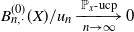 ;
; ;
; ;
;


where, as per (5.1), $({\rho}/{2})L^{0}_{t}(X)=\int_{0}^{t}\mathbf{1}_{\{X_s = 0\}}\,\mathrm{d}s$
for all
$({\rho}/{2})L^{0}_{t}(X)=\int_{0}^{t}\mathbf{1}_{\{X_s = 0\}}\,\mathrm{d}s$
for all $t\ge 0$
.
$t\ge 0$
.
Proof. Let Y be a sticky Brownian motion of stickiness parameter $\rho $
defined on the probability space
$\rho $
defined on the probability space $\mathcal{P}'_x = (\Omega',\mathcal{F}',(\mathcal{F}'_t)_{t\ge 0},\mathbb{P}'_x) $
such that,
$\mathcal{P}'_x = (\Omega',\mathcal{F}',(\mathcal{F}'_t)_{t\ge 0},\mathbb{P}'_x) $
such that, $\mathbb{P}'_x$
-a.s.,
$\mathbb{P}'_x$
-a.s., $Y_0 = x$
and Y is
$Y_0 = x$
and Y is $(\mathcal{F}'_t)_{t\ge 0}$
-adapted. We note that X and
$(\mathcal{F}'_t)_{t\ge 0}$
-adapted. We note that X and $|Y|$
are equal in law (see the discussion before the statement) and that
$|Y|$
are equal in law (see the discussion before the statement) and that
 \begin{align} B^{(0)}_{n,\cdot}(|Y|) & = B^{(0)}_{n,\cdot}(Y)+C^{(0)}_{n,\cdot}(Y), \nonumber\\ B^{(1)}_{n,\cdot}(|Y|) & = \mathbf{Z}^{(\,j)}_{n,\cdot}(Y) + B^{(0)}_{n,\cdot}(|Y|), \nonumber\\ B^{(2)}_{n,\cdot}(|Y|) & = \mathbf{Z}^{(\,j)}_{n,\cdot}(Y) + B^{(0)}_{n,\cdot}(|Y|). \end{align}
From Theorems 3.1 and 3.2, for every diverging sequence $(u_n)_n$
,
$(u_n)_n$
,

This, and the fact that $L^{0}_{t}(Y)= L^{0}_{t}(Y) \mathbf{1}_{\{L^{0}_{t}(Y)>0\}}$
an d
$L^{0}_{t}(Y)= L^{0}_{t}(Y) \mathbf{1}_{\{L^{0}_{t}(Y)>0\}}$
an d $L^{0}_{t}(|Y|)=2L^{0}_{t}(Y)$
, imply the convergences
$L^{0}_{t}(|Y|)=2L^{0}_{t}(Y)$
, imply the convergences

and

It is known that, in the case of constant limits, convergence in probability is equivalent to convergence in law (see [Reference Billingsley7, Theorem 25.2] and the discussion thereafter). And since $|Y|= X$
in law (which entails that
$|Y|= X$
in law (which entails that $(|Y|,L^{0}_{}(|Y|))=(X,L^{0}_{}(X))$
in law), the latter convergences hold with X instead of
$(|Y|,L^{0}_{}(|Y|))=(X,L^{0}_{}(X))$
in law), the latter convergences hold with X instead of $|Y|$
and
$|Y|$
and $\mathbb{P}_x$
instead of
$\mathbb{P}_x$
instead of $\mathbb{P}'_x$
. Therefore, again using that
$\mathbb{P}'_x$
. Therefore, again using that ${L^{0}_{t}(X)} = {L^{0}_{t}(X)} \mathbf{1}_{\{L^{0}_{t}(X)>0\}}$
, we obtain
${L^{0}_{t}(X)} = {L^{0}_{t}(X)} \mathbf{1}_{\{L^{0}_{t}(X)>0\}}$
, we obtain

and

Thus, we have

From Lemma 2.1, the convergences are uniform in time, in $\mathbb{P}_x$
-probability (
$\mathbb{P}_x$
-probability ( $\mathbb{P}_x$
-ucp). This proves (i), (ii), and (iii). From (5.4) and (5.5), we infer (iv). This completes the proof.
$\mathbb{P}_x$
-ucp). This proves (i), (ii), and (iii). From (5.4) and (5.5), we infer (iv). This completes the proof.
Corollary 5.1. We consider the setting of Theorem 5.1 and let $\mathcal H_t$
be the event
$\mathcal H_t$
be the event $\big\{\tau^{X}_0<t\big\} = \{$
there exists
$\big\{\tau^{X}_0<t\big\} = \{$
there exists $s \in [0,t) \colon X_s = 0\}$
. The statistic
$s \in [0,t) \colon X_s = 0\}$
. The statistic
 \begin{equation*} \varrho_n(X) = \bigg(4\sqrt{\frac2\pi}\bigg)\frac{1}{\sqrt{n}\,} \frac{\mathbf{Z}^{(2)}_{n,\cdot}(X)}{\mathbf{Z}^{(1)}_{n,\cdot}(X)} \end{equation*}
is a consistent estimator of $\rho$
, conditionally on the event
$\rho$
, conditionally on the event $\mathcal H_t$
, i.e.
$\mathcal H_t$
, i.e. $\varrho_n(X) \longrightarrow \rho$
, in
$\varrho_n(X) \longrightarrow \rho$
, in $\mathbb{P}^{\mathcal H_t}_x$
-probability, as
$\mathbb{P}^{\mathcal H_t}_x$
-probability, as $n \longrightarrow \infty$
.
$n \longrightarrow \infty$
.


5.2. Crossings and bouncings of sticky Itô diffusions
In this section we generalize Theorems 3.1 and 3.2 to sticky Itô diffusions. The generalization procedure is analogous to the ones in, e.g., [Reference Anagnostakis3, Reference Anagnostakis and Mazzonetto5, Reference Azas6, Reference Jacod21, Reference Mazzonetto27].
We consider the system

with $W_{}$
a standard Brownian motion, defined on the probability space
$W_{}$
a standard Brownian motion, defined on the probability space $\mathcal P_x = (\Omega, \mathcal{F}, (\mathcal{F}_t)_{t\ge 0},\mathbb{P}_x) $
such that,
$\mathcal P_x = (\Omega, \mathcal{F}, (\mathcal{F}_t)_{t\ge 0},\mathbb{P}_x) $
such that, $\mathbb{P}_x$
-a.s.,
$\mathbb{P}_x$
-a.s., $X_0=x$
. We suppose
$X_0=x$
. We suppose $(\mu,\sigma) $
satisfy the following conditions:
$(\mu,\sigma) $
satisfy the following conditions:
-
(c1) The diffusion coefficient
$\sigma$
is strictly positive and
$C^{1}$
. -
(c2) Weak existence and uniqueness in law holds for the system
(5.7)on
$\mathcal P_x$
such that,
$\mathbb{P}_x$
-a.s.,
$X'_0=x$
.
-
(c3) The laws of the solutions X, X ′ of (5.6) and (5.7) with the same initial condition (
$X_0 = X'_0 = x $
a.s.) are locally equivalent: they are mutually locally absolutely continuous in the sense of [Reference Jacod and Shiryaev24, Definition III.3.2]. Basically, this means for all
$t \ge 0$
,
$\mathrm{Law}\big(X|_{[0,t]}\big) \sim \mathrm{Law}\big(X'|_{[0,t]}\big)$
. Note that the processes are not necessarily defined on the same probability space. -
(c4) The state space of X ′ that solves (5.7) is an open interval J of
$\mathbb{R}$
, i.e. X
′ has only inaccessible boundaries (see, e.g., [Reference Kallenberg25, Section 33]).


Remark 5.1 Condition (c2) is equivalent to the weak existence and uniqueness for the classical SDE $\mathrm{d}X''_t = \sigma(X''_t)\,\mathrm{d}W_t$
. This is a consequence of, e.g., [Reference Anagnostakis3, Theorem 4.1] and [Reference Anagnostakis3, Proposition 4.2].
$\mathrm{d}X''_t = \sigma(X''_t)\,\mathrm{d}W_t$
. This is a consequence of, e.g., [Reference Anagnostakis3, Theorem 4.1] and [Reference Anagnostakis3, Proposition 4.2].
Under conditions (c1)–(c4), the following results hold.
Theorem 5.2. Let $C^{(0)}_{}$
,
$C^{(0)}_{}$
, $C^{(1)}_{}$
,
$C^{(1)}_{}$
, $C^{(2)}_{}$
,
$C^{(2)}_{}$
, $B^{(0)}_{}$
,
$B^{(0)}_{}$
, $B^{(1)}_{}$
,
$B^{(1)}_{}$
, $B^{(2)}_{}$
,
$B^{(2)}_{}$
, $\mathbf{Z}^{(1)}_{}$
, and
$\mathbf{Z}^{(1)}_{}$
, and $\mathbf{Z}^{(2)}_{}$
be the quantities defined in Section 1 for the process X. Then:
$\mathbf{Z}^{(2)}_{}$
be the quantities defined in Section 1 for the process X. Then:
-
(i) for every diverging sequence
$(u_n)_n$
, ; -
(ii)
; -
(iii)
,

 ;
; ;
; ,
, where, as per (5.6), $\rho L^{0}_{t}(X)=\int_{0}^{t}\mathbf{1}_{\{X_s = 0\}}\,\mathrm{d}s$
for all
$\rho L^{0}_{t}(X)=\int_{0}^{t}\mathbf{1}_{\{X_s = 0\}}\,\mathrm{d}s$
for all $t\ge 0 $
.
$t\ge 0 $
.
In the proof we reduce ourselves to the case of sticky Brownian motion. By the local equivalence in law (c3), it suffices to prove the result for (5.7). We then further reduce to the case of sticky Brownian motion by Girsanov’s lemma and a Lamperti transform.
Proof of Theorem
5.2. Let us first assume that the diffusion coefficient and its derivative satisfy the following conditions: there exists a real constant $\delta >0 $
such that, for all
$\delta >0 $
such that, for all $x \in \mathbb{R}$
,
$x \in \mathbb{R}$
, $\delta \le \sigma(x)\le 1/\delta$
and
$\delta \le \sigma(x)\le 1/\delta$
and $|\sigma'(x)| \le 1/\delta$
. We note that under these conditions, the state space J is
$|\sigma'(x)| \le 1/\delta$
. We note that under these conditions, the state space J is $\mathbb{R}$
. We consider X
′ to be the process that is the solution to (5.7), defined on
$\mathbb{R}$
. We consider X
′ to be the process that is the solution to (5.7), defined on $\mathcal P_x$
and with
$\mathcal P_x$
and with $(\mathcal{F}_t)_{t\ge 0}$
the natural filtration generated by X
′. By Definition 2.1 of ucp convergence, we can fix
$(\mathcal{F}_t)_{t\ge 0}$
the natural filtration generated by X
′. By Definition 2.1 of ucp convergence, we can fix $T>0$
and consider that all processes are restricted to the time interval [0,T].
$T>0$
and consider that all processes are restricted to the time interval [0,T].
Let $\mathcal{E}(\theta)$
,
$\mathcal{E}(\theta)$
, $\theta$
be the processes defined by
$\theta$
be the processes defined by
 \begin{equation*} \mathcal{E}_t(\theta) = \exp\bigg(\int_{0}^{t}\theta_s\,\mathrm{d}W_s - \frac{1}{2}\int_{0}^{t}\theta^2_s\,\mathrm{d}s\bigg), \qquad \theta_t = \frac12\sigma'(X_t), \quad t \ge 0. \end{equation*}
Since $\sigma'$
is bounded, from Girsanov’s theorem [Reference Anagnostakis3, Lemma 4.4] there exists a measure
$\sigma'$
is bounded, from Girsanov’s theorem [Reference Anagnostakis3, Lemma 4.4] there exists a measure $\mathbb{Q}_x$
such that the process
$\mathbb{Q}_x$
such that the process $(X'_t, W^{\theta}_{t})_{t\in [0,T]}$
jointly solves a drifted version of (5.7),
$(X'_t, W^{\theta}_{t})_{t\in [0,T]}$
jointly solves a drifted version of (5.7),

where $(W^{\theta}_{t})_{t\in [0,T]}$
is the
$(W^{\theta}_{t})_{t\in [0,T]}$
is the $\mathbb{Q}_x$
-Brownian motion defined by
$\mathbb{Q}_x$
-Brownian motion defined by $W^{\theta} = W_{} - \int_{0}^{\cdot}\theta_s\,\mathrm{d}s$
. Moreover, the Radon–Nikodym derivative
$W^{\theta} = W_{} - \int_{0}^{\cdot}\theta_s\,\mathrm{d}s$
. Moreover, the Radon–Nikodym derivative $\mathrm{d}\mathbb{Q}_x/\mathrm{d}\mathbb{P}_x|_{\mathcal{F}_T} = \mathcal{E}_T(\theta)$
.
$\mathrm{d}\mathbb{Q}_x/\mathrm{d}\mathbb{P}_x|_{\mathcal{F}_T} = \mathcal{E}_T(\theta)$
.
Let S be the function defined by
 \begin{equation*} S(y) = \int_{0}^{y} \frac{1}{\sigma(u)}\,\mathrm{d}u, \quad y \in \mathbb R. \end{equation*}
The function S is strictly increasing, $S(0)=0$
,
$S(0)=0$
, $S \in C^{2}(\mathbb{R})$
,
$S \in C^{2}(\mathbb{R})$
, $S'(y) = (\sigma(y))^{-1}$
, and
$S'(y) = (\sigma(y))^{-1}$
, and $S''(y) = -\sigma'(y)(\sigma(y))^{-2}$
,
$S''(y) = -\sigma'(y)(\sigma(y))^{-2}$
, $y \in \mathbb R$
. Let
$y \in \mathbb R$
. Let $Y'_{} \;:\!=\; S(X')$
, Then, from the Itô–Tanaka formula (see, e.g., [Reference Anagnostakis3, Lemma 4.5]), (5.8), and the fact that
$Y'_{} \;:\!=\; S(X')$
, Then, from the Itô–Tanaka formula (see, e.g., [Reference Anagnostakis3, Lemma 4.5]), (5.8), and the fact that $S(0)=0$
,
$S(0)=0$
, $(Y'_{}, W^{\theta}_{})$
solves
$(Y'_{}, W^{\theta}_{})$
solves

From characterization (p2), the process Y
′ is a sticky Brownian motion under $\mathbb{Q}_x$
of stickiness parameter
$\mathbb{Q}_x$
of stickiness parameter $\rho\sigma(0)$
and Theorems 3.1 and 3.2 do apply to Y
′ for the probability
$\rho\sigma(0)$
and Theorems 3.1 and 3.2 do apply to Y
′ for the probability $\mathbb{Q}_x$
. In particular:
$\mathbb{Q}_x$
. In particular:
-
(i)
, -
(ii)
, -
(iii)
.
 ,
, ,
, .
. Since S is strictly increasing and $S(0)=0$
,
$S(0)=0$
,
-
• for all n, t and
$j\in\{0,1,2\}$
,
$C^{(\,j)}_{n,t}(Y'_{}) = C^{(\,j)}_{n,t}(X')$
,
$B^{(\,j)}_{n,t}(Y'_{}) = B^{(\,j)}_{n,t}(X')$
, -
• for all n, t and
$j\in \{1,2\} $
,
$\mathbf{Z}^{(\,j)}_{n,t}(Y'_{}) = \mathbf{Z}^{(\,j)}_{n,t}(X') $
, -
• for all i, n,
$U^{n}_{i}(Y'_{})=U^{n}_{i}(X') $
,






and, $\mathbb{Q}_x $
-a.s.,
$\mathbb{Q}_x $
-a.s., $L^{0}_{t}(X') = \sigma(0)L^{0}_{t}(Y'_{})$
. From the equivalence of measure
$L^{0}_{t}(X') = \sigma(0)L^{0}_{t}(Y'_{})$
. From the equivalence of measure $\mathbb{P}_x \sim \mathbb{Q}_x$
when restricted to
$\mathbb{P}_x \sim \mathbb{Q}_x$
when restricted to $\mathcal{F}_T$
, and the fact that
$\mathcal{F}_T$
, and the fact that $\mathcal E(\theta)_T $
is an exponential martingale (even square integrable), we deduce that the previous convergences also hold under
$\mathcal E(\theta)_T $
is an exponential martingale (even square integrable), we deduce that the previous convergences also hold under $\mathbb{P}_x$
. The proof is thus completed for (5.7) under the boundedness assumptions on the diffusion coefficient and its derivative.
$\mathbb{P}_x$
. The proof is thus completed for (5.7) under the boundedness assumptions on the diffusion coefficient and its derivative.
Let us consider a standard localization argument to go from bounded to unbounded $\sigma$
,
$\sigma$
, $1/\sigma$
, and
$1/\sigma$
, and $\sigma'$
by considering
$\sigma'$
by considering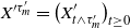 $X'^{\tau'_m} = \big(X'_{t\wedge \tau'_m}\big)_{t\ge 0}$
. More precisely, let
$X'^{\tau'_m} = \big(X'_{t\wedge \tau'_m}\big)_{t\ge 0}$
. More precisely, let $(\mathcal{F}_t)_{t\ge 0}$
be the filtration generated by X
′, let
$(\mathcal{F}_t)_{t\ge 0}$
be the filtration generated by X
′, let $(K_m)_m $
be an increasing sequence of compacts of J such that
$(K_m)_m $
be an increasing sequence of compacts of J such that $\bigcup_m K_m = J $
, and let
$\bigcup_m K_m = J $
, and let $(\tau'_m)_m $
be the sequence of stopping times defined by
$(\tau'_m)_m $
be the sequence of stopping times defined by $\tau'_m = \inf\{t\ge 0\colon X'_t \not\in K_m \}$
and
$\tau'_m = \inf\{t\ge 0\colon X'_t \not\in K_m \}$
and $X'^{\tau'_m} $
be the stopped process, defined by
$X'^{\tau'_m} $
be the stopped process, defined by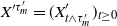 $X'^{\tau'_m} = (X'_{t\wedge \tau'_m})_{t\ge 0} $
. Condition (c4) ensures that
$X'^{\tau'_m} = (X'_{t\wedge \tau'_m})_{t\ge 0} $
. Condition (c4) ensures that
 \begin{equation} \lim_{m \rightarrow \infty} \mathbb{P}_x(t > \tau'_m) = 0 \end{equation}
for all $t\geq 0$
. For a process Z and all
$t\geq 0$
. For a process Z and all $t\geq 0$
, let
$t\geq 0$
, let $(\,f_n(Z,t))_n$
be a sequence of statistics such that
$(\,f_n(Z,t))_n$
be a sequence of statistics such that $f_n(Z,t)$
is
$f_n(Z,t)$
is $\mathcal{F}_t $
-measurable. These quantities represent the difference between the statistics of interest and their limits. We also observe that
$\mathcal{F}_t $
-measurable. These quantities represent the difference between the statistics of interest and their limits. We also observe that
 \begin{equation*} \begin{aligned} \mathbb{P}_x (|\,f_n(X',t)|>\varepsilon) & \le \mathbb{P}_x(|\,f_n(X',t)|>\varepsilon;\, t\le \tau'_m) + \mathbb{P}_x(t > \tau'_m) \\ & = \mathbb{P}_x(|\,f_n(X',t \wedge \tau'_m)|>\varepsilon;\, t\le \tau'_m) + \mathbb{P}_x(t > \tau'_m). \end{aligned} \end{equation*}
We use the previous part to pass to the limit as $n\to \infty$
. Next, we let
$n\to \infty$
. Next, we let $m \longrightarrow \infty$
. From (5.9), this proves the result for X
′.
$m \longrightarrow \infty$
. From (5.9), this proves the result for X
′.
From (c3), these convergences also hold in $\mathbb{P}_x$
-probability for the solution to (5.6).
$\mathbb{P}_x$
-probability for the solution to (5.6).
From Lemma 2.1, the convergence is also uniform in time, in $\mathbb{P}_x$
-probability (
$\mathbb{P}_x$
-probability ( $\mathbb{P}_x$
-ucp). This completes the proof.
$\mathbb{P}_x$
-ucp). This completes the proof.
Corollary 5.2. Let $\mathcal P_x =(\Omega, \mathcal{F}, (\mathcal{F}_t)_{t\ge 0}, \mathbb{P}_x)$
be a filtered probability space and let X be an
$\mathcal P_x =(\Omega, \mathcal{F}, (\mathcal{F}_t)_{t\ge 0}, \mathbb{P}_x)$
be a filtered probability space and let X be an $(\mathcal{F}_t)_{t\ge 0}$
-adapted process solution to (5.6) on
$(\mathcal{F}_t)_{t\ge 0}$
-adapted process solution to (5.6) on $\mathcal P_x$
. The statistic defined by
$\mathcal P_x$
. The statistic defined by
 \begin{equation*} \varrho_n(X) = \bigg(\frac{4}{\sigma(0)}\sqrt{\frac2\pi}\bigg)\frac{1}{\sqrt{n}\,} \frac{C^{(2)}_{n,t}(X)}{C^{(1)}_{n,t}(X)}, \quad n \in \mathbb{N}, \end{equation*}
is a consistent estimator of $\rho$
, conditionally on the event
$\rho$
, conditionally on the event $\mathcal H_t = \{\tau^{X}_0 < t\} = \{$
there exists
$\mathcal H_t = \{\tau^{X}_0 < t\} = \{$
there exists $s \in [0,t) \colon X_s = 0\}$
. This means that (see Definition 2.2),
$s \in [0,t) \colon X_s = 0\}$
. This means that (see Definition 2.2), $\varrho_n(X) \longrightarrow \rho$
, in
$\varrho_n(X) \longrightarrow \rho$
, in $\mathbb{P}^{\mathcal H_t}_x $
-probability, as
$\mathbb{P}^{\mathcal H_t}_x $
-probability, as $n \longrightarrow \infty$
.
$n \longrightarrow \infty$
.
Proof. The proof is the same as the proof of Proposition 3.2, using Theorem 5.2 instead of Theorem 3.1. We should also justify that, $\mathbb{P}_x$
-a.s.,
$\mathbb{P}_x$
-a.s., $\mathcal H_t = \{L^{0}_{t}(X) > 0\}$
. For this, it suffices to remark that, as seen in the proof of Proposition 3.2, this is the case for sticky Brownian motion, so using the notations of the proof of Theorem 5.2, for Y under
$\mathcal H_t = \{L^{0}_{t}(X) > 0\}$
. For this, it suffices to remark that, as seen in the proof of Proposition 3.2, this is the case for sticky Brownian motion, so using the notations of the proof of Theorem 5.2, for Y under $\mathbb{Q}_x$
. From [Reference Revuz and Yor30, Exercise VI.1.23], this is the case for
$\mathbb{Q}_x$
. From [Reference Revuz and Yor30, Exercise VI.1.23], this is the case for $X = S^{-1}(Y)$
under
$X = S^{-1}(Y)$
under $\mathbb{Q}_x $
. From the equivalence of probability measures, this is also the case for X under
$\mathbb{Q}_x $
. From the equivalence of probability measures, this is also the case for X under $\mathbb{P}_x $
. This completes the proof.
$\mathbb{P}_x $
. This completes the proof.
Remark 5.2. Corollary 5.2 holds by replacing $(C^{(1)}_{n,t}(X),C^{(2)}_{n,t}(X))$
with
$(C^{(1)}_{n,t}(X),C^{(2)}_{n,t}(X))$
with $(\mathbf{Z}^{(1)}_{n,t}(X),\mathbf{Z}^{(2)}_{n,t}(X))$
.
$(\mathbf{Z}^{(1)}_{n,t}(X),\mathbf{Z}^{(2)}_{n,t}(X))$
.
6. Numerical experiments
In this section we aim to numerically establish the properties of the stickiness parameter estimator $\varrho_n$
devised in Proposition 3.2. We compare it with the stickiness parameter estimator
$\varrho_n$
devised in Proposition 3.2. We compare it with the stickiness parameter estimator $\varrho^{(0)}_n $
of [Reference Anagnostakis and Mazzonetto5] (recalled in (3.1)) in terms of variance and convergence rate.
$\varrho^{(0)}_n $
of [Reference Anagnostakis and Mazzonetto5] (recalled in (3.1)) in terms of variance and convergence rate.
We simulate sample paths of the sticky Brownian motion of stickiness parameter $\rho=1$
. For this, we use the STMCA approximation scheme with the tuned grid defined in [Reference Anagnostakis, Lejay and Villemonais4, Section 2.3] of size criteria
$\rho=1$
. For this, we use the STMCA approximation scheme with the tuned grid defined in [Reference Anagnostakis, Lejay and Villemonais4, Section 2.3] of size criteria $h=0.005$
(the nomenclature tuned grid and size criteria is as used in [Reference Anagnostakis, Lejay and Villemonais4] – it is a grid adapted to the diffusion we aim to approximate). This ensures good convergence properties of the scheme [Reference Anagnostakis, Lejay and Villemonais4, Corollary 2.5]. We consider initial value
$h=0.005$
(the nomenclature tuned grid and size criteria is as used in [Reference Anagnostakis, Lejay and Villemonais4] – it is a grid adapted to the diffusion we aim to approximate). This ensures good convergence properties of the scheme [Reference Anagnostakis, Lejay and Villemonais4, Corollary 2.5]. We consider initial value $X_0 = 0 $
and time horizon
$X_0 = 0 $
and time horizon $T=1 $
.
$T=1 $
.
Stickiness parameter estimation for the sticky Brownian motion: $\varrho$
vs.
$\varrho$
vs. $\varrho^{(0)}$
. Simulation size:
$\varrho^{(0)}$
. Simulation size: $N_{\mathrm{MC}}= 2000$
. High values of
$N_{\mathrm{MC}}= 2000$
. High values of $\alpha,n$
induce some bias in the approximation due to the grid nature of the STMCA approximation scheme (see the discussion in [Reference Anagnostakis, Lejay and Villemonais4]).
$\alpha,n$
induce some bias in the approximation due to the grid nature of the STMCA approximation scheme (see the discussion in [Reference Anagnostakis, Lejay and Villemonais4]).

For each generated path $\widetilde X^{(i)} $
we consider the Monte Carlo estimators of
$\widetilde X^{(i)} $
we consider the Monte Carlo estimators of $\rho$
given by
$\rho$
given by
 \begin{equation*} \mu_{\mathrm{MC}} \;:\!=\; \frac{1}{N_{\mathrm{MC}}}\sum_{i=1}^{N_{\mathrm{MC}}}\varrho_{n}(\widetilde X^{(i)}), \qquad \mu^{(0)}_{\mathrm{MC}} \;:\!=\; \frac{1}{N_{\mathrm{MC}}}\sum_{i=1}^{N_{\mathrm{MC}}}\varrho_{n}^{(0)}(\widetilde X^{(i)}),\end{equation*}
where $N_{\mathrm{MC}} $
is the Monte Carlo simulation size and the estimator
$N_{\mathrm{MC}} $
is the Monte Carlo simulation size and the estimator $\varrho^{(0)}_n$
, defined in (3.1), is considered for test function
$\varrho^{(0)}_n$
, defined in (3.1), is considered for test function $g\colon [x \rightarrow \mathbf{1}_{\{0<|x|<5\}}/10] $
and
$g\colon [x \rightarrow \mathbf{1}_{\{0<|x|<5\}}/10] $
and $u_n = n^{\alpha} $
for different values of
$u_n = n^{\alpha} $
for different values of $\alpha$
close to
$\alpha$
close to $0.5$
. For Brownian motion
$0.5$
. For Brownian motion $\alpha=0.5$
yields a higher convergence speed [Reference Jacod21].
$\alpha=0.5$
yields a higher convergence speed [Reference Jacod21].
We also consider the associated Monte Carlo variance estimators
 \begin{align*} \sigma_{\mathrm{MC}} \;:\!=\; \Bigg(\frac{1}{N_{\mathrm{MC}}}\sum_{i=1}^{N_{\mathrm{MC}}}(\varrho_{n}(\widetilde X^{(i)}) - \mu_{\mathrm{MC}})^{2}\Bigg)^{1/2}, \\ \sigma^{(0)}_{\mathrm{MC}} \;:\!=\; \Bigg(\frac{1}{N_{\mathrm{MC}}}\sum_{i=1}^{N_{\mathrm{MC}}} \big(\varrho^{(0)}_{n}(\widetilde X^{(i)}) - \mu^{(0)}_{\mathrm{MC}}\big)^{2}\Bigg)^{1/2}.\end{align*}
The numerical simulations indicate that the choice of the normalizing sequence affects the overall convergence rate of $\varrho^{(0)}_{n}(X) $
. Compared to
$\varrho^{(0)}_{n}(X) $
. Compared to $\varrho^{(0)}_{n}(X) $
, the estimator
$\varrho^{(0)}_{n}(X) $
, the estimator $\varrho_{n}(X) $
has the advantage that it does not depend upon a test function and a normalizing sequence. Moreover, the numerical simulations indicate the following:
$\varrho_{n}(X) $
has the advantage that it does not depend upon a test function and a normalizing sequence. Moreover, the numerical simulations indicate the following:
-
• The estimator
$\varrho $
seems superior to
$\varrho^{(0)} $
for any normalizing sequence as it has less variance (see Table 1; also compare Table 2 with [Reference Anagnostakis3, Table 2]). -
• The Monte Carlo standard deviation decreases as a function of the sampling frequency n (see Table 2).


A theoretical analysis of the convergence speed is the object of further research.
Stickiness parameter estimation of the sticky Brownian motion using the estimator $\varrho$
: variance as function of n. Simulation size:
$\varrho$
: variance as function of n. Simulation size: $N_{\mathrm{MC}}= 5000$
.
$N_{\mathrm{MC}}= 5000$
.

Appendix A. Proof of Lemma 4.1
For the reader’s convenience, we recall the statement of Lemma 4.1. Let us also recall that we consider the notation of (2.2)–(2.4) in Proposition 2.1.
Lemma. Consider the setting of Theorem 3.1. Let $(\,f_n,k_n,g_n,h_n;\,n\in\mathbb{N})$
be the functions defined for all
$(\,f_n,k_n,g_n,h_n;\,n\in\mathbb{N})$
be the functions defined for all $n \in \mathbb{N}$
and
$n \in \mathbb{N}$
and $x\in \mathbb{R}$
by
$x\in \mathbb{R}$
by $f_n(x) \;:\!=\; \mathbb{P}_{x}(X_{1/n} = 0)$
,
$f_n(x) \;:\!=\; \mathbb{P}_{x}(X_{1/n} = 0)$
, $k_n(x) \;:\!=\; \mathbf{1}_{\{x\not = 0\}}\,f_n(x/\sqrt n)$
,
$k_n(x) \;:\!=\; \mathbf{1}_{\{x\not = 0\}}\,f_n(x/\sqrt n)$
, $g_n(x) \;:\!=\; \mathbb{P}_{x}(xX_{1/n} < 0)$
, and
$g_n(x) \;:\!=\; \mathbb{P}_{x}(xX_{1/n} < 0)$
, and $h_n(x) \;:\!=\; \sqrt n g_n(x/\sqrt n)$
. Then:
$h_n(x) \;:\!=\; \sqrt n g_n(x/\sqrt n)$
. Then:
-
(i)
$\lim_{n \rightarrow \infty}f_n(0) = 1$
and
$\lim_{n \rightarrow \infty}\sqrt n(1- f_n(0)) = {2\sqrt{2}}/{\rho\sqrt\pi}$
; -
(ii) the sequence
$(k_n)_n $
satisfies (2.3) and
$\lim_{n \rightarrow \infty}m_{\sqrt n\rho}(k_n) = 2\sqrt{{2}/{\pi}}$
; -
(iii) the sequence
$(h_n)_n $
satisfies (2.3) and
$\lim_{n \rightarrow \infty}m_{\sqrt n\rho}(h_n) = 1/{\rho}$
.






Let us also recall some useful results.
Lemma A.1. (For example, [Reference Borodin and Salminen8, p. 124].) The probability transition kernel of the sticky Brownian motion of stickiness parameter $\rho$
with respect to its speed measure
$\rho$
with respect to its speed measure $m_{\rho}(\mathrm{d}y) = \mathrm{d}y + \rho\,\delta_0(\mathrm{d}y)$
is the function defined for all
$m_{\rho}(\mathrm{d}y) = \mathrm{d}y + \rho\,\delta_0(\mathrm{d}y)$
is the function defined for all $t>0$
and
$t>0$
and $x,y\in\mathbb{R}$
by
$x,y\in\mathbb{R}$
by
 \begin{equation*} p_{\rho}(t,x,y) = \frac{{\mathrm{e}}^{-(x-y)^2/2t} - {\mathrm{e}}^{-(|x|+|y|)^2/2t}}{\sqrt{2 \pi t}} + \frac{1}{\rho}{\mathrm{e}}^{2(|x|+|y|)/\rho + 2t/\rho^2} \mathrm{erfc}\bigg(\frac{|x|+|y|}{\sqrt{2t}} + \frac{\sqrt{2t}}{\rho}\bigg). \end{equation*}
Lemma A.2. (For example, [Reference Anagnostakis3, Corollary 2.7].) The probability transition kernel of the sticky Brownian motion with respect to its speed measure $m_{\rho}(\mathrm{d}x) = \mathrm{d}x + \rho\,\delta_0(\mathrm{d}x)$
satisfies, for all
$m_{\rho}(\mathrm{d}x) = \mathrm{d}x + \rho\,\delta_0(\mathrm{d}x)$
satisfies, for all $c,\rho,t>0$
and
$c,\rho,t>0$
and $x,y\in \mathbb{R}$
,
$x,y\in \mathbb{R}$
, $p_{\rho}(ct,x,y)\,m_{\rho}(\mathrm{d}y) = p_{\rho/\sqrt{c}}(t,x/\sqrt{c},y)\,m_{\rho/\sqrt{c}}(\mathrm{d}y)$
.
$p_{\rho}(ct,x,y)\,m_{\rho}(\mathrm{d}y) = p_{\rho/\sqrt{c}}(t,x/\sqrt{c},y)\,m_{\rho/\sqrt{c}}(\mathrm{d}y)$
.
We are now ready to provide the proof of Lemma 4.1. From Lemma A.2, for all $n\in \mathbb{N} $
and
$n\in \mathbb{N} $
and $x\in \mathbb{R} $
, we have
$x\in \mathbb{R} $
, we have

Proof of item (i). Regarding the first relation, from (A.1) and Lemma A.1,
 \begin{equation*} f_n(0) = (\sqrt n \rho)p_{\sqrt n \rho }(1,0,0) = {\mathrm{e}}^{2/n\rho^2}\mathrm{erfc}\bigg(\frac{\sqrt{2}}{\sqrt n\rho}\bigg). \end{equation*}
Taking the limit as $n \longrightarrow \infty$
yields the result. Indeed, we have
$n \longrightarrow \infty$
yields the result. Indeed, we have
 \begin{equation*} \lim_{n \rightarrow \infty} f_n(0) = \lim_{y \rightarrow 0} e^{y^{2}} \mathrm{erfc}(y) = 1. \end{equation*}
Regarding the second relation, from the l’Hôspital’s rule,
 \begin{equation*} \lim_{y \rightarrow 0}\frac{1}{y}\big(1 - {\mathrm{e}}^{y^{2}}\mathrm{erfc}(y)\big) = -\lim_{y \rightarrow 0}{\mathrm{e}}^{y^{2}}\mathrm{erfc}'(y) = \frac{2}{\sqrt{\pi}\,}. \end{equation*}
Taking the limit as $n \longrightarrow \infty$
yields
$n \longrightarrow \infty$
yields
 \begin{equation*} \lim_{n \rightarrow \infty}\sqrt n(1 - f_n(0)) = \lim_{n \rightarrow \infty}\frac{\sqrt{2}}{\rho}\bigg(\frac{\sqrt{2}}{\sqrt{n}\rho}\bigg)^{-1}(1 - f_n(0)) = \frac{\sqrt{2}}{\rho}\frac{2}{\sqrt{\pi}\,} = \frac{2}{\rho}\sqrt{\frac{2}{\pi}}, \end{equation*}
which is the desired result. This completes the proof.
Proof of item (ii). Since $k_n(0)=0$
, from (A.1) and Lemma A.1 we have
$k_n(0)=0$
, from (A.1) and Lemma A.1 we have
 \begin{equation*} \begin{aligned} m_{\sqrt n \rho}( k_n ) = \int_{\mathbb{R}}k_n(x)\,\mathrm{d}x & = (\sqrt n\rho)\int_{\mathbb{R}}p_{\sqrt n\rho}(1,x,0)\,\mathrm{d}x \\ & = \int_{\mathbb{R}}{\mathrm{e}}^{2|x|/\sqrt n\rho + 2/n\rho^2} \mathrm{erfc}\bigg(\frac{|x|}{\sqrt{2}\,} + \frac{\sqrt{2}}{\sqrt n\rho}\bigg)\,\mathrm{d}x. \end{aligned} \end{equation*}
Regarding the function we integrate, from the Mills ratio on the Gaussian random variable (see [Reference Grimmett and Stirzaker18, p. 98]), for some constant $K_{\mathrm{Mills}}>0$
, we have
$K_{\mathrm{Mills}}>0$
, we have
 \begin{equation*} \begin{aligned} \lim_{n \rightarrow \infty}{\mathrm{e}}^{2|x|/\sqrt n\rho + 2/n\rho^2} \mathrm{erfc}\bigg(\frac{|x|}{\sqrt{2}\,} + \frac{\sqrt{2}}{\sqrt n\rho}\bigg) & = \mathrm{erfc}\bigg(\frac{|x|}{\sqrt{2}\,}\bigg), \\ \mathbf{1}_{\{|x|\ge 1\}}{\mathrm{e}}^{2|x|/\sqrt n\rho + 2/n\rho^2} \mathrm{erfc}\bigg(\frac{|x|}{\sqrt{2}\,} + \frac{\sqrt{2}}{\sqrt n\rho}\bigg) & \le \mathbf{1}_{\{|x|\ge 1\}}K_{\mathrm{Mills}}\frac{\sqrt{2n}\rho}{\sqrt n\rho|x|+ 2} \mathrm{erfc}\bigg({-}\frac{x^{2}}{2}\bigg) \\ & \le \sqrt{2}K_{\mathrm{Mills}}\mathrm{erfc}\bigg({-}\frac{x^{2}}{2}\bigg), \\ \mathbf{1}_{\{|x|< 1\}}{\mathrm{e}}^{2|x|/\sqrt n\rho + 2/n\rho^2} \mathrm{erfc}\bigg(\frac{|x|}{\sqrt{2}\,} + \frac{\sqrt{2}}{\sqrt n\rho}\bigg) & \le \mathbf{1}_{\{|x|<1\}}{\mathrm{e}}^{2/\rho + 2/\rho^{2}}\mathrm{erfc}\bigg(\frac{|x|}{\sqrt{2}\,}\bigg), \end{aligned} \end{equation*}
where both upper bounds are $L^{1}(\mathbb{R})$
. Thus, from the dominated convergence theorem,
$L^{1}(\mathbb{R})$
. Thus, from the dominated convergence theorem,
 \begin{equation*} \lim_{n \rightarrow \infty}m_{\sqrt n\rho}(k_n) = \lim_{n \rightarrow \infty}\int_{\mathbb{R}}\mathrm{erfc}\bigg(\frac{|x|}{\sqrt{2}\,}\bigg)\,\mathrm{d}x = 2\sqrt{\frac{2}{\pi}}. \end{equation*}
This proves the second assertion.
Regarding the first assertion, we observe that

where the upper bound defines a function in $L^{1}(\mathbb{R})$
. Hence, from the dominated convergence theorem,
$L^{1}(\mathbb{R})$
. Hence, from the dominated convergence theorem,
 \begin{equation*} \begin{aligned} \lim_{n \rightarrow \infty}{\int_{-\infty}^{+\infty}|x|k_n(x)\,\mathrm{d}x} & = \int_{\mathbb{R}}\lim_{n \rightarrow \infty}\bigg(|x|{\mathrm{e}}^{2|x|/\sqrt n\rho + 2/n\rho^2} \mathrm{erfc}\bigg(\frac{|x|}{\sqrt{2}\,} + \frac{\sqrt{2}}{\sqrt n\rho}\bigg)\bigg)\,\mathrm{d}x \\ & = \int_{\mathbb{R}}|x|\mathrm{erfc}\bigg(\frac{|x|}{\sqrt{2}\,}\bigg)\,\mathrm{d}x = 1. \end{aligned} \end{equation*}
With similar arguments, we can prove that $m(k^{2}_n)$
converges to some constant
$m(k^{2}_n)$
converges to some constant $K > 0$
. Also,
$K > 0$
. Also,
 \begin{equation*} \lim_{n \rightarrow \infty}k^{2}_n(\sqrt nx) = \lim_{n \rightarrow \infty} \bigg({\mathrm{e}}^{2|x|/\rho + 2/n\rho^2}\mathrm{erfc}\bigg(\frac{\sqrt n|x|}{\sqrt{2}\,} + \frac{\sqrt{2}}{\sqrt n\rho}\bigg)\bigg)^{2} = 0. \end{equation*}
From all the above, $(k_n)_n $
satisfies (2.3). This completes the proof.
$(k_n)_n $
satisfies (2.3). This completes the proof.
Proof of item (iii). The first assertion is proved with similar arguments to the proof of item (ii). Regarding the second assertion, from (A.1) and Lemma A.1, we have
 \begin{equation*} \begin{aligned} & \sqrt n\mathbf{1}_{\{xy<0\}}p_{\sqrt n\rho}(1,x,y) \\ & \quad = \frac{1}{\rho}\mathbf{1}_{\{xy<0\}}\big(\mathbf{1}_{\{|x|+|y|\ge 1\}}+\mathbf{1}_{\{|x|+|y|< 1\}}\big) {\mathrm{e}}^{2(|x|+|y|)/\sqrt n\rho + 2/n\rho^2}\mathrm{erfc}\bigg(\frac{|x|+|y|}{\sqrt{2}\,} + \frac{\sqrt{2}}{\sqrt n\rho}\bigg) \\ & \quad \le 2\bigg(\mathbf{1}_{\{|x|+|y|\ge 1\}}K_{\mathrm{Mills}} \frac{\sqrt{2n}\rho(|x|+|y|)}{\sqrt n\rho(|x|+|y|)+ 2}{\mathrm{e}}^{-({(|x|+|y|)^{2}})/{2}} \\ & \quad\qquad + \mathbf{1}_{\{|x|+|y|<1\}}{\mathrm{e}}^{2/\rho + 2/\rho^{2}} \mathrm{erfc}\bigg(\frac{|x|+|y|}{\sqrt{2}}\bigg)\bigg) \\ & \quad \le 2\bigg(\mathbf{1}_{\{|x|+|y|\ge 1\}}K_{\mathrm{Mills}}\sqrt{2}{\mathrm{e}}^{-({(|x|+|y|)^{2}})/{2}} + \mathbf{1}_{\{|x|+|y|<1\}}{\mathrm{e}}^{2/\rho + 2/\rho^{2}}\mathrm{erfc}\bigg(\frac{|x|+|y|}{\sqrt{2}}\bigg)\bigg), \end{aligned} \end{equation*}
where the upper bound defines a function in $L^{1}(\mathbb{R})$
. Hence, from the dominated convergence theorem,
$L^{1}(\mathbb{R})$
. Hence, from the dominated convergence theorem,

This completes the proof.
Appendix B. Proof of Lemma 4.3
For reader’s convenience, we recall the statement of Lemma 4.3 using the notation in (4.3) for the first hitting time.
Lemma. (Reflection principle for sticky Brownian motion) Let X be the sticky Brownian motion of stickiness parameter $\rho>0$
defined on the filtered probability space
$\rho>0$
defined on the filtered probability space $\mathcal P_x = (\Omega, \mathcal{F}, (\mathcal{F}_t)_{t\ge 0},\mathbb{P}_x)$
such that,
$\mathcal P_x = (\Omega, \mathcal{F}, (\mathcal{F}_t)_{t\ge 0},\mathbb{P}_x)$
such that, $\mathbb{P}_x$
-a.s.,
$\mathbb{P}_x$
-a.s., $X_0 = x$
(in particular, X is
$X_0 = x$
(in particular, X is $(\mathcal F_t)_{t\ge 0}$
-adapted). Let X
′ be the process defined, for all
$(\mathcal F_t)_{t\ge 0}$
-adapted). Let X
′ be the process defined, for all $t\ge 0$
, by
$t\ge 0$
, by

The process X
′ defined this way is a sticky Brownian motion of stickiness parameter $\rho$
.
$\rho$
.
Proof. Let Z be the Brownian motion defined in characterization (t1) on an extension of the probability space, so that, for all $t \ge 0$
,
$t \ge 0$
, $X_t = Z_{\gamma(t)}$
with
$X_t = Z_{\gamma(t)}$
with $\gamma$
the time change defined in (t1). We observe that
$\gamma$
the time change defined in (t1). We observe that $\tau^{X}_{0}=\gamma(\tau^{Z}_{0})$
. Let Z
′ be the process defined for all
$\tau^{X}_{0}=\gamma(\tau^{Z}_{0})$
. Let Z
′ be the process defined for all $t\ge 0 $
by
$t\ge 0 $
by

From the reflection principle of the Brownian motion Z (see [Reference Revuz and Yor30, Exercise III.3.14]), Z
′ is also a Brownian motion. Moreover, $L^{0}_{}(Z)=L^{0}_{}(Z')$
,
$L^{0}_{}(Z)=L^{0}_{}(Z')$
, $\tau^{Z}_0=\tau^{Z'}_0$
. Therefore,
$\tau^{Z}_0=\tau^{Z'}_0$
. Therefore, $A(t)=t+\rho L^{0}_{t}(Z')$
and
$A(t)=t+\rho L^{0}_{t}(Z')$
and $\tau^{X}_0=\gamma\big(\tau^{Z}_0\big)=\gamma\big(\tau^{Z'}_0\big)$
which, by the definition of X
′, is also equal to
$\tau^{X}_0=\gamma\big(\tau^{Z}_0\big)=\gamma\big(\tau^{Z'}_0\big)$
which, by the definition of X
′, is also equal to $\tau^{X'}_0$
. From all the above, we show that
$\tau^{X'}_0$
. From all the above, we show that $X' = \big(Z'_{\gamma(t)}\big)_{t\ge 0}$
. Indeed, on the event
$X' = \big(Z'_{\gamma(t)}\big)_{t\ge 0}$
. Indeed, on the event $\big\{t\geq \tau^{X}_0\big\}$
we have
$\big\{t\geq \tau^{X}_0\big\}$
we have
 \begin{equation*} X_t'= -X_t = - Z_{\gamma(t)} = (-Z)_{\gamma(t)} = Z'_{\gamma(t)}, \end{equation*}
and, since $X_t=Z_{\gamma(t)}$
,
$X_t=Z_{\gamma(t)}$
, $X'_t = Z_{\gamma(t)}\mathbf{1}_{\{t < \tau^{X}_0\}} + Z'_{\gamma(t)}\mathbf{1}_{\{t\geq \tau^{X}_0\}} = Z'_{\gamma(t)}$
. To finish the proof, it suffices to observe that (t2) ensures that X
′ is a sticky Brownian motion of stickiness parameter
$X'_t = Z_{\gamma(t)}\mathbf{1}_{\{t < \tau^{X}_0\}} + Z'_{\gamma(t)}\mathbf{1}_{\{t\geq \tau^{X}_0\}} = Z'_{\gamma(t)}$
. To finish the proof, it suffices to observe that (t2) ensures that X
′ is a sticky Brownian motion of stickiness parameter $\rho$
.
$\rho$
.
Funding information
The authors were partially supported by the Programme Exploratoire Pluridisciplinaire (PEPS) of CNRS Mathématiques.
Competing interests
There were no competing interests to declare which arose during the preparation or publication process of this article.