

1. Introduction
The coast of mainland Norway is dominated by the presence of fjords. Often subjected to air temperatures below freezing, sea ice has the possibility to form in these regions. The larger fjords are mostly ice free in winter due to the inflow of warm oceanic water, but ice often forms in the inner parts of fjords and fjord arms, with variable duration and extent of the ice cover (Eilertsen and Skardhamar, Reference Eilertsen and Skardhamar2006). It is understood that one condition important, often necessary, for ice to form in fjords is a layer of brackish water on the surface (Gade, Reference Gade and Hurdle1986). This water can be less dense than the warmer ocean water below, leading to little vertical mixing and a stable water column that promotes cooling and ice formation at the surface (Manak and Mysak, Reference Manak and Mysak1989; Ogi and Tachibana, Reference Ogi and Tachibana2001). Calm oceanic and atmospheric conditions must be present to allow for the stratified water column to form. These requirements of fresh water and calm conditions make ice formation a local effect, likely to vary between fjords and years.
Very little systematic work has been done on ice in mainland Norwegian fjords. The Norwegian pilot guide offers brief descriptions of ice extent in selected fjords to assist boat and ship captains (Hughes, Reference Hughes2006). However, the guide is based primarily on limited data with little focus on interannual variability. There is a wide breadth of work examining Norwegian fjords from physical and biological perspectives (e.g. Hopkins and others, Reference Hopkins, Tande and Grønvik1984; Stigebrandt and Aure, Reference Stigebrandt and Aure1989; Svendsen, Reference Svendsen1995; Asplin and others, Reference Asplin, Salvanes and Kristoffersen1999; Eilertsen and Skardhamar, Reference Eilertsen and Skardhamar2006; Skardhamar and others, Reference Skardhamar2018). In these works, focus is primarily placed on the warmer, summer months with ice conditions in the winter mentioned only occasionally. One can turn to research focused on fjords found in Arctic regions such as Svalbard which have been closely investigated regarding sea ice (Cottier and others, Reference Cottier, Nilsen, Skogseth, Tverberg, Skarðhamar and Svendsen2010; Nilsen and others, Reference Nilsen, Cottier, Skogseth and Mattsson2008; Smedsrud and Skogseth, Reference Smedsrud and Skogseth2006). These regions differ from coastal Norway, given longer periods of cooler temperatures.
Ice can alter the physical behavior of a fjord, i.e. the transmission of light through the water column and heat flux from the air to ocean and vice versa, and in turn alter biological conditions (Gradinger, Reference Gradinger2009; Arndt and Nicolaus, Reference Arndt and Nicolaus2014; Arrigo and others, Reference Arrigo2014). In addition, ice can create an obstacle to those transiting certain areas by boat – slowing speed, increasing risk in search and rescue scenarios and complicating the clean-up of any spilled pollutants such as oil (Arctic Marine Shipping Assessment, 2009). With industry increasing in the North, a larger number of boats and people are being drawn to these areas. Understanding ice conditions including not only where ice may be present but the properties of that ice, i.e. thickness, porosity and permeability, will better prepare northern communities for future development (Petrich and others, Reference Petrich2019). Previous work has examined the relationship of oceanic, atmospheric and hydrologic variables to ice extent in estuaries and other areas where rivers interact with marine environments; however, little focus has been placed on the Norwegian coastline (Manak and Mysak, Reference Manak and Mysak1989; Ogi and Tachibana, Reference Ogi and Tachibana2001; Granskog and others, Reference Granskog, Ehn and Niemelä2005; Kuzyk and others, Reference Kuzyk, Macdonald, Granskog and Scharien2008). Here we first present findings of ice extent determined from the analysis of Moderate Resolution Imaging Spectroradiometer (MODIS) satellite images from 2001 through 2019, February through May for each year, with focus placed on fjords but including coastal areas where similar oceanic and weather conditions may exist enabling ice formation. We next examine correlations between ice extent and several variables related to weather: air temperature, new snowfall and rainfall plus snowmelt.
2. Data and Methods
2.1 Analysis of imagery and measurement of ice extent
Many of the fjords along the Norwegian coastline are narrow (<2 km wide), with steep slopes, and often experience cloudy weather; 24 h darkness also occurs in the northern-most regions. For these reasons, remote sensing of fjords along the Norwegian coast can be challenging. In a previous study examining ice cover in the northern Norwegian fjord of Porsangerfjorden, false color images were manually examined to determine changes in ice extent through time (Petrich and others, Reference Petrich, O'Sadnick and Dale2017). Here, a similar approach is taken but automated using Google Earth Engine.
The MOD09A1.006 Surface Reflectance 8-Day Global 500 m dataset was chosen to be analyzed (Vermote, Reference Vermote2015). This dataset provides surface spectral reflectance values of Terra, a NASA satellite that began collecting environmental data in 2000, MODIS bands 1 through 7 with corrections for atmospheric conditions including gasses and aerosols. For each pixel, one value is chosen over an 8-day period based on cloud cover and solar zenith. Given the frequency of cloud cover along coastal Norway, an instrument performing daily passes is ideal. Additionally, through using the 8-day composite, corrections are made to decrease, but do not remove all, the possible influence of clouds on results. If several pixels over the 8-day period are found to be of equal quality, the one having the lowest reflectance in channel 3 is used. To illuminate ice, the following formula was applied:
Ice Index = Band 3 – (Band 6 + Band 7).
These three bands are commonly used in false color images. Band 3, in the visible part of the spectrum (459–479 nm), reflects well off ice while Band 6 (1628–1652 nm) and Band 7 (2105–2155 nm) are both absorbed. Reflectance in the latter two is indicative of cloud cover, of concern given the possibility of cloud cover in these regions over periods of time longer than the 8-day time span composite is created. Thus, by using the three bands in combination, ice is illuminated while further minimizing the impact of cloud cover on results. To ensure only ice on the ocean surface was considered and no pixels of snow-covered land or in-land ice were included, the MOD44W.005 Land Water Mask was applied. Having a resolution of 250 m, this mask is derived from the MODIS and Shuttle Radar Topography Mission (SRTM) data (Carroll and others, Reference Carroll2017).
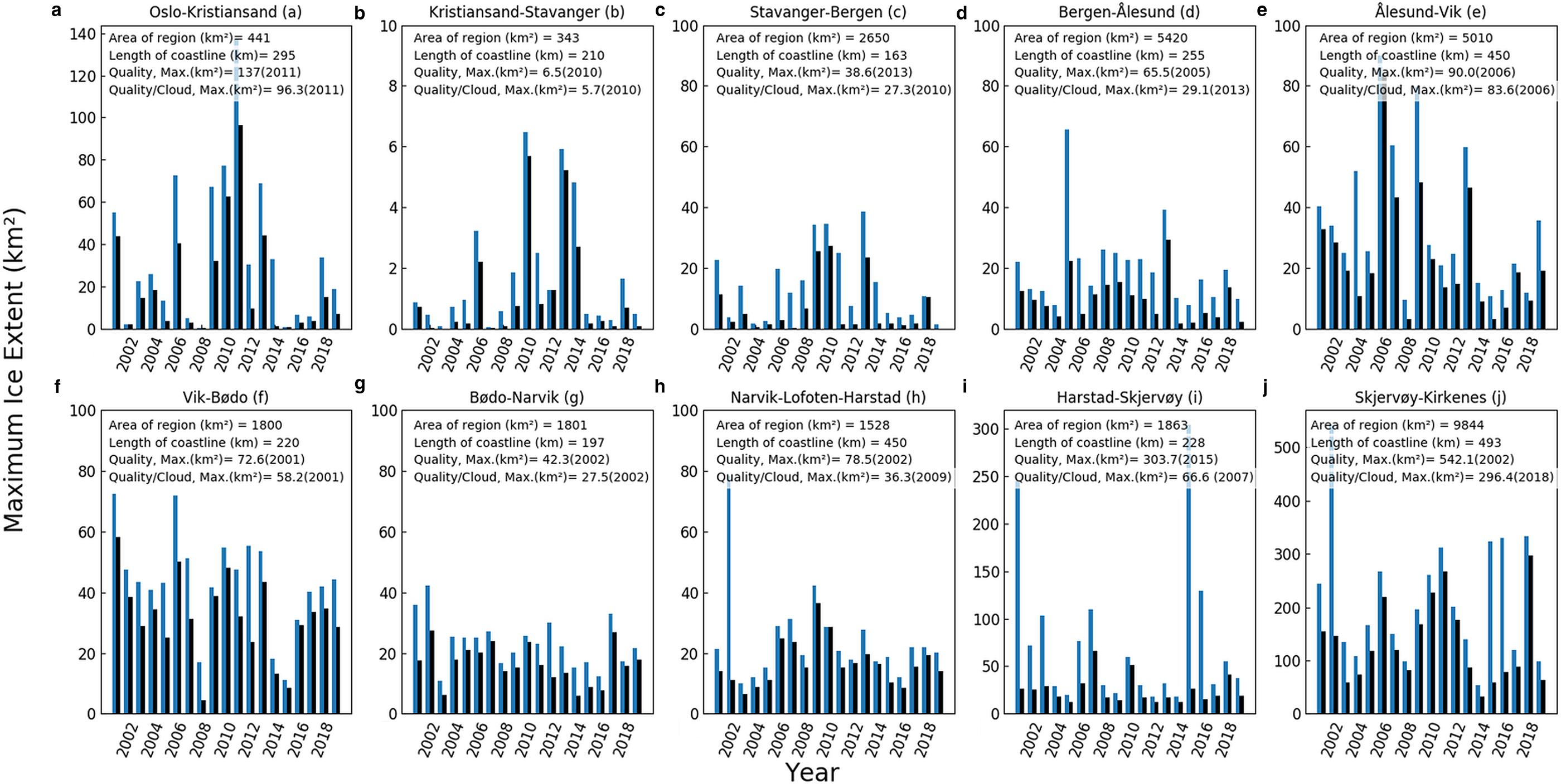
Prior to the calculation of ice extent, all images were filtered based on quality and cloud cover using Quality Assessment (QA) and State Quality Assessment (StateQA) data, respectively. For QA data, the first 30 bits were examined with only pixels defined as being of ‘ideal quality’ for all bands included in analysis, thus filtering out any pixels marked as ‘less than ideal quality’ or not corrected for atmospheric effects due to clouds. For StateQA data, the first three bits were processed which provide a description of cloud state and cloud shadow. Pixels were filtered to include only those having a ‘clear’ cloud state (as opposed to ‘cloudy’, ‘mixed’, ‘not set’) and no cloud shadow. The majority of the following analysis was completed using results from images filtered using both QA and StateQA data. A comparison to results produced when only QA data were used is still provided however due to the observed frequency of cloud cover by the authors in northern Norway in wintertime (Fig. 3). Filtering using QA and StateQA may result in an underestimation despite the 8-day composite being used to select images with the lowest cloud cover. On average, ice extent was 38% lower in results filtered using both QA and StateQA data. The four most southern regions, Oslo–Kristiansand, Kristiansand–Stavanger, Stavanger–Bergen and Bergen–Ålesund, showed the greatest similarity between the two types of filtering, falling below this average. The remaining six regions were above.
For analysis, focus was placed primarily on fjords but also included several narrow channels and areas with a high density of small islands and inlets. Smaller fjords/inlets were also often grouped together (Figs 1 and 2) given the length of the coastline. A region of interest (ROI) was created around each, a total of 386, with boundaries determined subjectively by the coastline and natural breaks (i.e. abrupt changes in fjord width, direction, etc.). Each ROI was drawn manually in Google Earth Engine using the polygon tool to output a geometry object and are specific for use in this work, not being used previously. Pixels that are partially (>0.50%) within the ROI are weighted based on the fraction of the pixel included in the region. Visually inspecting the land mask shows generally good agreement, but areas where there is not perfect alignment are evident. This can introduce an overestimation due to land being mistaken as water with snow cover being identified as ice. Through creating ROIs that follow the coastline closely, the possibility of misidentification is further prevented. In addition, through normalization of ice extent by maximum ice extent, any remaining error is lessened assuming more constant conditions (snow or no snow) on land than in the water. Any fjords having an ice extent >5 km2 were also manually examined to further ensure accurate results.
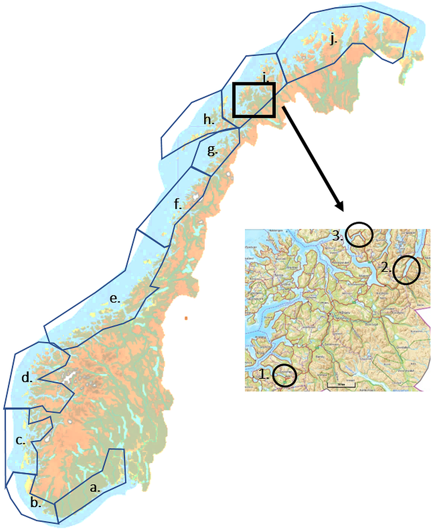
Norwegian coastline with regions used for analysis outlined. (a) Oslo–Kristiansand; (b) Kristiansand–Stavanger; (c) Stavanger–Bergen; (d) Bergen–Ålesund; (e) Ålesund–Vik; (f) Vik–Bodø; (g) Bodø–Narvik; (h) Narvik–Lofoten–Harstad; (i) Harstad–Skjervøy; (j) Skjervøy–Kirkenes. The boxed area shows the three fjords examined closer, (1) Gratangsbotn, (2) Storfjord and (3) Sørbotn/Ramfjord.
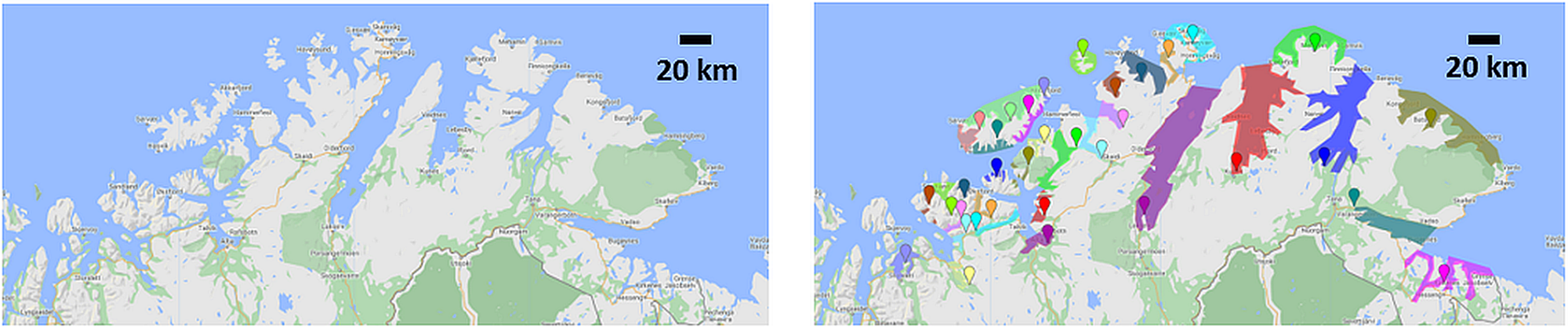
Example of region-of-interest (ROI) placement and point selection for weather data for the Skjervøy–Kirkenes (j) region.
To determine ice extent, the number of pixels within each ROI having an ice band value above 0.3 were counted. Given an array of ice (e.g. homogeneous snow covered, meltwater, bare ice) and atmospheric conditions, setting a threshold proved non-trivial. Depending on the region and fjord, ice band values for pixels holding ice could vary from where the threshold was set, 0.3, upwards to ~0.7. Pixels with high reflectances (indicative of ice) in band 3 also could have high values in bands 6 and 7. The result often led to ice band values between 0.2 and 0.3; however, while such a pixel could have held ice, clouds were also possibly present influencing results. Such pixels were often filtered out using StateQA data; however, by applying the 0.3 threshold, further reassurance is provided that only ice is counted.
The sum of pixels holding ice was multiplied by the area of the pixel, often varying slightly from 0.25 km2 (expected for a 500 m pixel) given MODIS is produced in a geographic coordinate system and referenced to a spheroid. The calculation was done at a scale of 500 m, the average value of a pixel within the spheroid and the resolution of the MOD09 dataset. The land mask was therefore downscaled to a lower resolution. For fjords above the Arctic Circle, no images are gathered between 1 November and 2 February. Values of maximum ice extent therefore apply to ice observed between 2 February and 24 May. It is important to note however that ice may have been present and extended further during the period no images were gathered.
For every fjord/coastal area, a maximum ice extent for each year of analysis, 2001–2019, was obtained. These data acted as a starting point to determine if any significant trends existed as well as revealed the spread of values for ice extent in individual fjords, highlighting which showed particularly high extent, >5 km2. Given the large number of fjords outlined, the majority of analysis here is presented with ROIs grouped into regions, created based primarily on features in the coastline (Figs 1 and 2), namely Oslo–Kristiansand (a), Kristiansand–Stavanger (b), Stavanger–Bergen (c), Bergen–Ålesund (d), Ålesund–Vik (e), Vik–Bodø (f), Bodø–Narvik (g), Narvik–Lofoten–Harstad (h), Harstad–Skjervøy (i) and Skjervøy–Kirkenes (j). Through grouping the numerous ROIs, analysis can begin examining the variations between years and possible causes, potentially directing future studies where individual fjords are examined. To provide an example of how regional findings may differ from that of individual fjords, three fjords from the Harstad–Skjervøy region were selected Gratangsbotn (a), Storfjord (b) and Sørbotn/Ramfjord (c) (Fig. 1).
Ice extent was summed between all fjords in a region for each date included in the time span investigated, with a maximum ice extent found for each year (Fig. 3). For each region, the yearly maximum was normalized by the highest maximum of ice extent observed from 2001 through 2019. This was done for results obtained when images were filtered using only QA data, to remove pixels of poor quality, and QA and StateQA data, to remove pixels of poor quality and those with clouds present. The normalized ice extent for each region was used in the subsequent analysis comparing ice extent to ancillary data.
Maximum ice area for each region and year with comparison between filtering methods using only quality, QA, data (blue) and quality and cloud, QA and StateQA, data (black). The area, length of outer coastline and maximums for both filtering approaches are also provided for each region. (a) Oslo–Kristiansand; (b) Kristiansand–Stavanger; (c) Stavanger–Bergen; (d) Bergen–Ålesund; (e) Ålesund–Vik; (f) Vik–Bodø; (g) Bodø–Narvik; (h) Narvik–Lofoten–Harstad; (i) Harstad–Skjervøy; (j) Skjervøy–Kirkenes. Note, while the y-axis scale is generally consistent, it differs on plots for regions (b), (i) and (j).
2.2 Analysis of ancillary data
The relationship was examined between ice extent and two variables enabling fjord ice formation, cold weather and a source of fresh water. Estimates of daily new snowfall, daily snow melt and rainfall, and daily average temperature were obtained through seNorge (Lussana and others, Reference Lussana, Tveito and Uboldi2016). This open online database provides several datasets including rain, snow and temperature used most often for the monitoring and prediction of hazards including avalanches, floods and landslides. Data are only available for land-based locations. Temperature data are interpolated at 1 km resolution from point observations from ~230 measurement stations across Norway. Values for daily rainfall plus snowmelt in millimeters provide an estimate of total water supply and are based on point measurements from ~400 stations that are interpolated onto a 1 km grid (Engeset, Reference Engeset2016). Daily new snowfall in millimeters is provided by the Norwegian Water Resources and Energy Directorate (NVE) and is calculated from models using the temperature and precipitation data described above. Both snow and weather data have a resolution of 1 km and a time resolution of 24 h.
Given unknowns as to where runoff may end up and subsequently mix with fjord water, total runoff from the catchment area around a fjord was not considered. Representative temperature, new snowfall, and rainfall plus snowmelt data for each region were obtained by selecting one point at the head of each fjord near to sea level for all contained in each region (Fig. 2). Through using only one location from each fjord/coastal area, an understanding of the general weather patterns and their potential impact on fresh water in the fjord for a given year is provided. This allows for examination of how such weather patterns may influence ice formation without introducing unknown artifacts, for example, some fjords may have strong gradients in temperature throughout the fjord while others not as much, some fjords may have many river inlets while others only have one main source of water. Using the approach outlined here, an understanding of the general weather patterns and their influence on ice extent over the time span examined can begin to form with findings useful in future studies focused on specific regions or weather variables.
For correlation analysis, cumulative daily new snowfall and daily rainfall plus snowmelt were calculated from 1 November to 30 April of each year. This range of dates differs from the period ice extent is examined to account for the possible influence of snowfall and rainfall/snowmelt prior to freeze-up. Freezing degree days (FDD), the sum of average daily temperatures below 0°C, was determined during this time period as well. As fresh water may enable formation, the freezing temperature of fresh water (0°C) was set as the threshold to calculate FDD, although this may vary depending on the fjord and timing of freeze-up in relation to weather events (e.g. Weeks and Ackley Reference Weeks and Ackley1982).
3. Results
3.1 Maximum ice extent in fjords
While the majority of the analysis presented here focuses on the ten selected regions, results from individual fjords and areas along the coast were also examined to understand if and how many contributed most to higher values of ice extent. Often this led to manually sorting through images to ensure accuracy. Of the 386 fjords/coastal areas examined, 47 had over 5 km2 of ice during at least one season between 2001 and 2019. The majority of areas with high ice extent were found in the Skjervøy–Kirkenes region, 22 out of 47, while Ålesund–Vik came in second with seven out of 47. Additionally, Vik–Bodø had five out of 47; Bergen–Ålesund had four out of 47; Oslo–Kristiansand, Stavanger–Bergen, Narvik–Lofoten–Harstad and Harstad–Skjervøy all had two each out of 47; and Bodø–Narvik had one. While these values are driven by the overall area of the ROI (the reason why the following results are presented normalized), they provide context for where ice may be expected and to what degree. Additionally, such findings motivate the continuing analysis of why some fjords/coastal areas display years with high extent and relatedly, how ice varies through a season and between years and the main contributing factors.
3.2 Trends in regional ice extent
3.2.1 Trends from 2001 to 2019
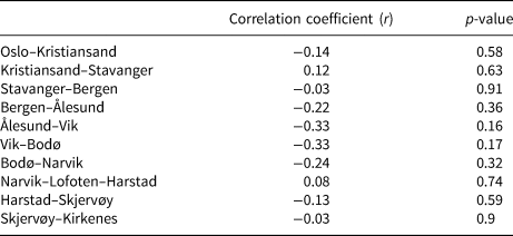
No statistically significant trend (p < 0.05) was found between ice extent and variations between 2001 and 2019 when a linear least-squared trend regression analysis was performed (Table 1). Between years and through individual seasons however, variations were observed sometimes consistently and sometimes unique to each region. In the following, the factors driving these findings are of focus.
Results from linear least-squared regression trend analysis for ice extent by region from 2001–2019
3.2.2 Patterns in seasonal and interannual ice extent
Depending on the year, the area of ice in a region was non-existent, increased and decreased gradually, or showed abrupt changes between images (Fig. 7). In the southern three regions, Oslo–Kristiansand (a), Kristiansand–Stavanger (b) and Stavanger–Bergen (c), several years revealed a total ice extent <0.20 the maximum or no ice at all (Fig. 4). For example, 2007 was a year of very low ice extent in these three regions. Additionally, between 2014 and 2017, regions (a), (b) and (c) have had ice extents consistently lower than 0.50 the maximum. In 2018, ice extent increased but returned to similarly low values in 2019. The next two regions, Bergen–Ålesund (d) and Ålesund–Vik (e), also show a similar pattern but with longer periods having a small area of ice each year.
Total ice extent, determined using QA and StateQA filtering, in each region for dates 2 February through 24 May, 2001 through 2019 normalized by the maximum ice extent measured during this time period. (a) Oslo-Kristiansand, (b) Kristiansand-Stavanger, (c) Stavanger–Bergen, (d) Bergen–Ålesund, (e) Ålesund–Vik, (f) Vik–Bodø, (g) Bodø–Narvik, (h) Narvik–Lofoten–Harstad, (i) Harstad–Skjervøy, (j) Skjervøy–Kirkenes.
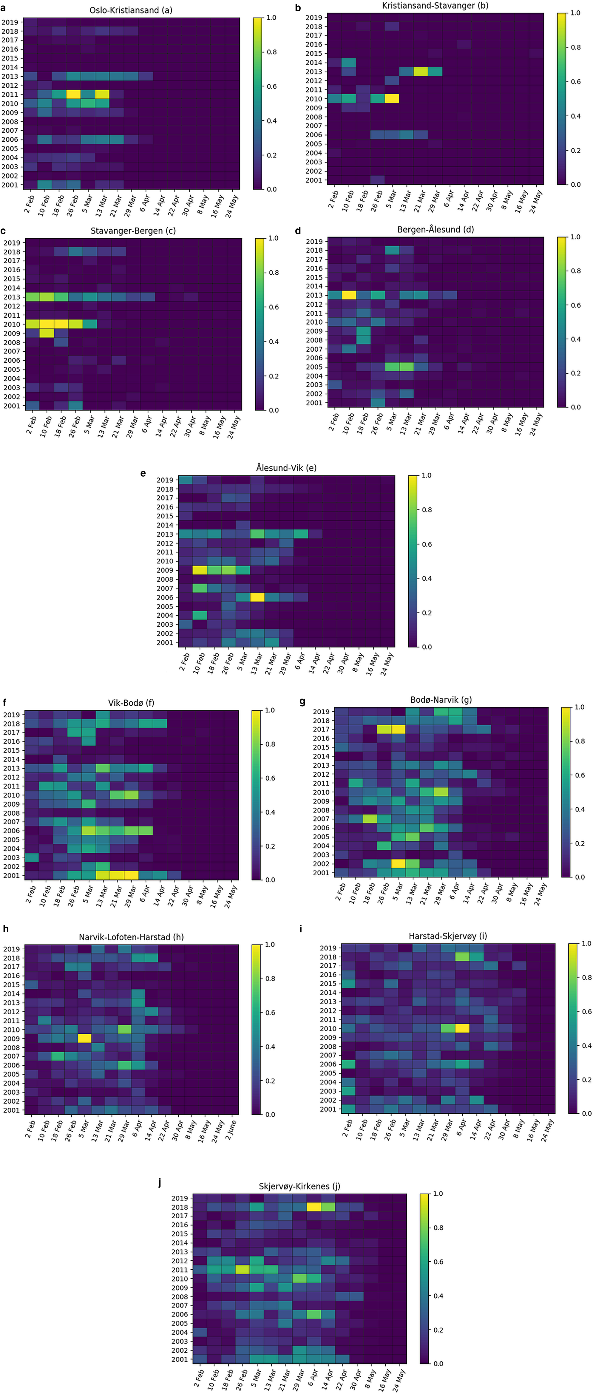
For the regions of Vik–Bodø (f), Bodø–Narvik (g), Narvik–Lofoten–Harstad (h), Harstad–Skjervøy (i) and Skjervøy–Kirkenes (j), ice is consistently observed each year over varying lengths of time. Gradual increases and decreases in ice extent were also more commonly observed in these regions, for example, in 2006 where all five regions generally increased to a maximum between 21 March and 6 April before a decrease. Additionally, further north, measured ice extent was more consistent between years with yearly maximum ice extent often above 0.50–0.60 of the overall maximum. Harstad–Skjervøy (i) region differs slightly with 2010 and 2018 showing noticeable extremes with all other years being more similar in total ice extent being 40–60% of the maximum.
In regions (a), (b) and (c), outside of 2013, ice was not measured after March except at very low quantities. In regions (d) and (e), the period of time where ice was observed extended into the first 2 weeks of April with the possibility of ice at very low values until May (Fig. 4). Further north, in the regions (f) and (g), ice was often found at higher quantities at the beginning of April but showed low values by 30 April with very little observed in May. The remaining two regions, (f) and (j), revealed ice seasons extending more frequently into May but with very little ice measured after 16 May.
3.3 Correlation of maximum ice extent with weather variables
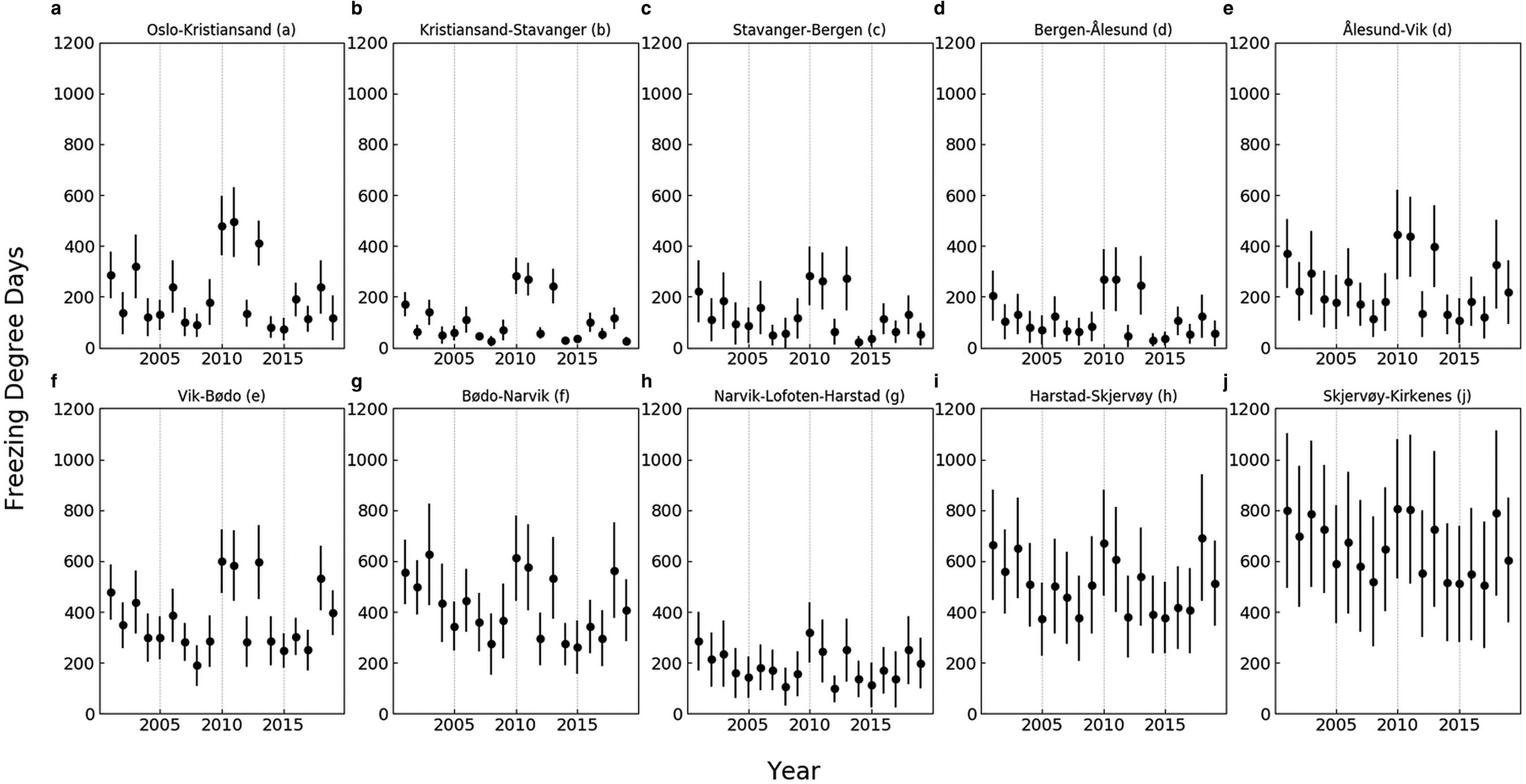
For each fjord/coastal area in a region, FDD, cumulative daily new snowfall and daily rainfall plus snowmelt were calculated. The values in Figs 5–7 represent an average over all areas within a region with std dev. also determined.
Average freezing degree days for each region and year, calculated between 1 November and 30 April, with bars representing std dev.. (a) Oslo–Kristiansand; (b) Kristiansand–Stavanger; (c) Stavanger–Bergen; (d) Bergen–Ålesund; (e) Ålesund–Vik; (f) Vik–Bodø; (g) Bodø–Narvik; (h) Narvik–Lofoten–Harstad; (i) Harstad–Skjervøy; (j) Skjervøy–Kirkenes.

Average sum of rainfall plus snowmelt for each region and year, calculated between 1 November and 30 April, with bars representing std dev. (a) Oslo–Kristiansand; (b) Kristiansand–Stavanger; (c) Stavanger–Bergen; (d) Bergen–Ålesund; (e) Ålesund–Vik; (f) Vik–Bodø; (g) Bodø–Narvik; (h) Narvik–Lofoten–Harstad; (i) Harstad–Skjervøy; (j) Skjervøy–Kirkenes.

Average sum of snowfall for each region and year, calculated between 1 November and 30 April, with bars representing std dev. (a) Oslo–Kristiansand; (b) Kristiansand–Stavanger; (c) Stavanger–Bergen; (d) Bergen–Ålesund; (e) Ålesund–Vik; (f) Vik–Bodø; (g) Bodø–Narvik; (h) Narvik–Lofoten–Harstad; (i) Harstad–Skjervøy; (j) Skjervøy–Kirkenes.

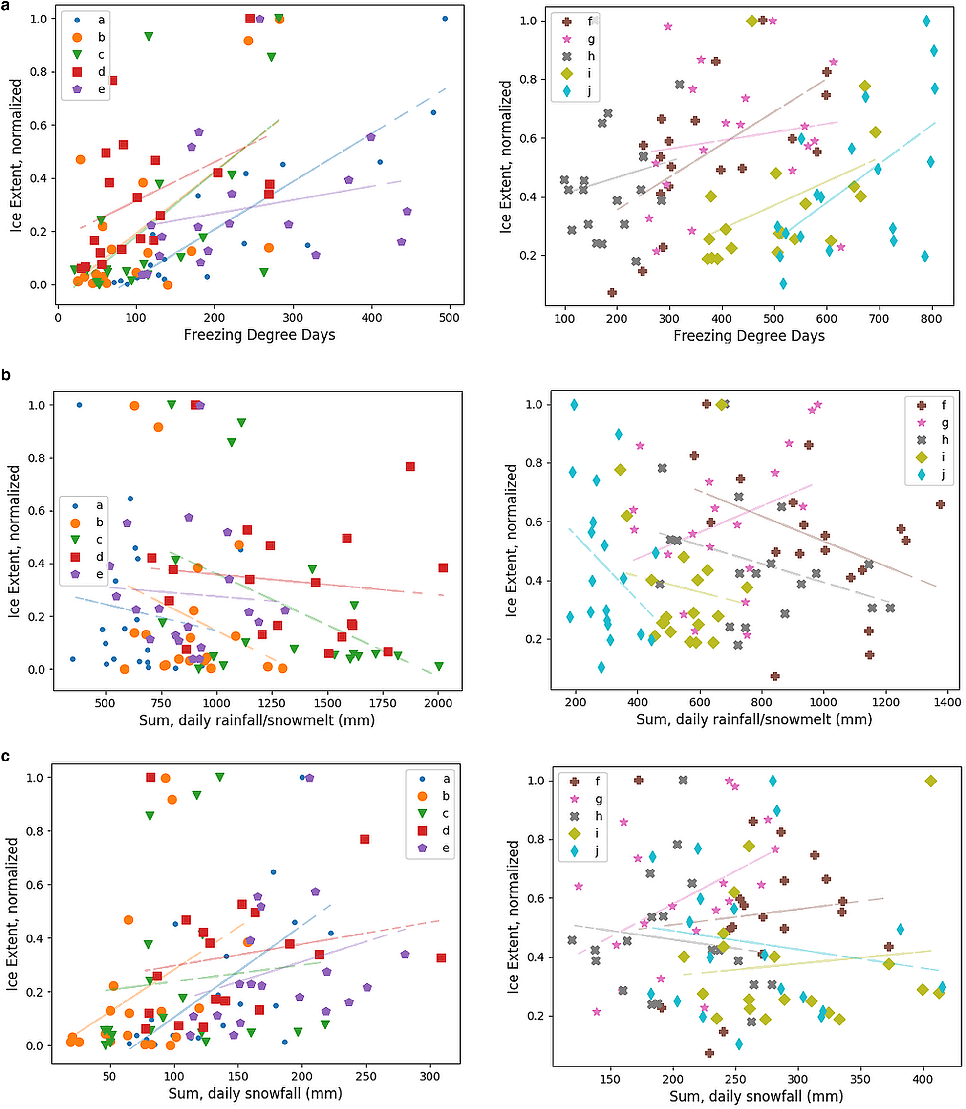
A Pearson's correlation coefficient (r) and p-value were calculated between each variable – daily snowfall, daily rainfall plus snowmelt and FDD – in comparison to maximum ice extent from 2 February and 24 May (Fig. 8, Table 2). Four out of the ten regions examined – Oslo–Kristiansand (a), Kristiansand–Stavanger (b), Stavanger–Bergen (c) and Vik–Bodø (d) – had a significant correlation between ice extent and FDD (p-value <0.05) when both filtering methods were used (Fig. 8a, Table 2). Two additional regions – Bergen–Ålesund (d) and Skjervøy–Kirkenes (j) – showed a significant correlation only when images were filtered using QA and StateQA data. Lastly, Harstad–Skjervøy (i) showed a correlation to FDD but of slightly lower significance, p = 0.078. The three regions that showed no significant correlation to FDD were Ålesund–Vik (e), Bodø–Narvik (f) and Narvik–Lofoten–Harstad (i). Significant correlations to the two other variables presented were less frequent. Stavanger–Bergen (c) showed a significant negative correlation to rain plus snowmelt using both filtering methods (Fig. 8b, Table 2). Both Oslo–Kristiansand (a) and Bodø–Narvik (g) showed a significant correlation to snowfall, the latter only when using QA/StateQA filtering (Fig. 8c, Table 2). Seven out of ten regions showed good agreement between the two filtering methods used. The three regions where filtering by QA/StateQA versus only QA showed disagreement resulting in no significant correlation were Bergen–Ålesund (d), Narvik–Lofoten–Harstad (h) and Harstad–Skjervøy (i).
Normalized ice extent filtered using QA and StateQA data compared to (a) freezing degree days, (b) sum of daily rainfall plus snowmelt and (c) sum of daily new snowfall for regions. A linear trend line for each region is included to highlight the relationship between and spread of data points. (a) Oslo–Kristiansand; (b) Kristiansand–Stavanger; (c) Stavanger–Bergen; (d) Bergen–Ålesund; (e) Ålesund–Vik; (f) Vik–Bodø; (g) Bodø–Narvik; (h) Narvik–Lofoten–Harstad; (i) Harstad–Skjervøy; (j) Skjervøy–Kirkenes.
Pearson's correlation coefficient and p-value between ice extent and three variables for each region
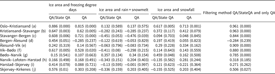
Significant correlations (p < 0.05) marked in gray. Those with 0.05> p < 0.1 marked in light gray. (a) Oslo–Kristiansand; (b) Kristiansand–Stavanger; (c) Stavanger–Bergen; (d) Bergen–Ålesund; (e) Ålesund–Vik; (f) Vik–Bodø; (g) Bodø–Narvik; (h) Narvik–Lofoten–Harstad; (i) Harstad–Skjervøy; (j) Skjervøy–Kirkenes.
3.4 Selected fjords in the Harstad–Skjervøy region
3.4.1 Ice extent
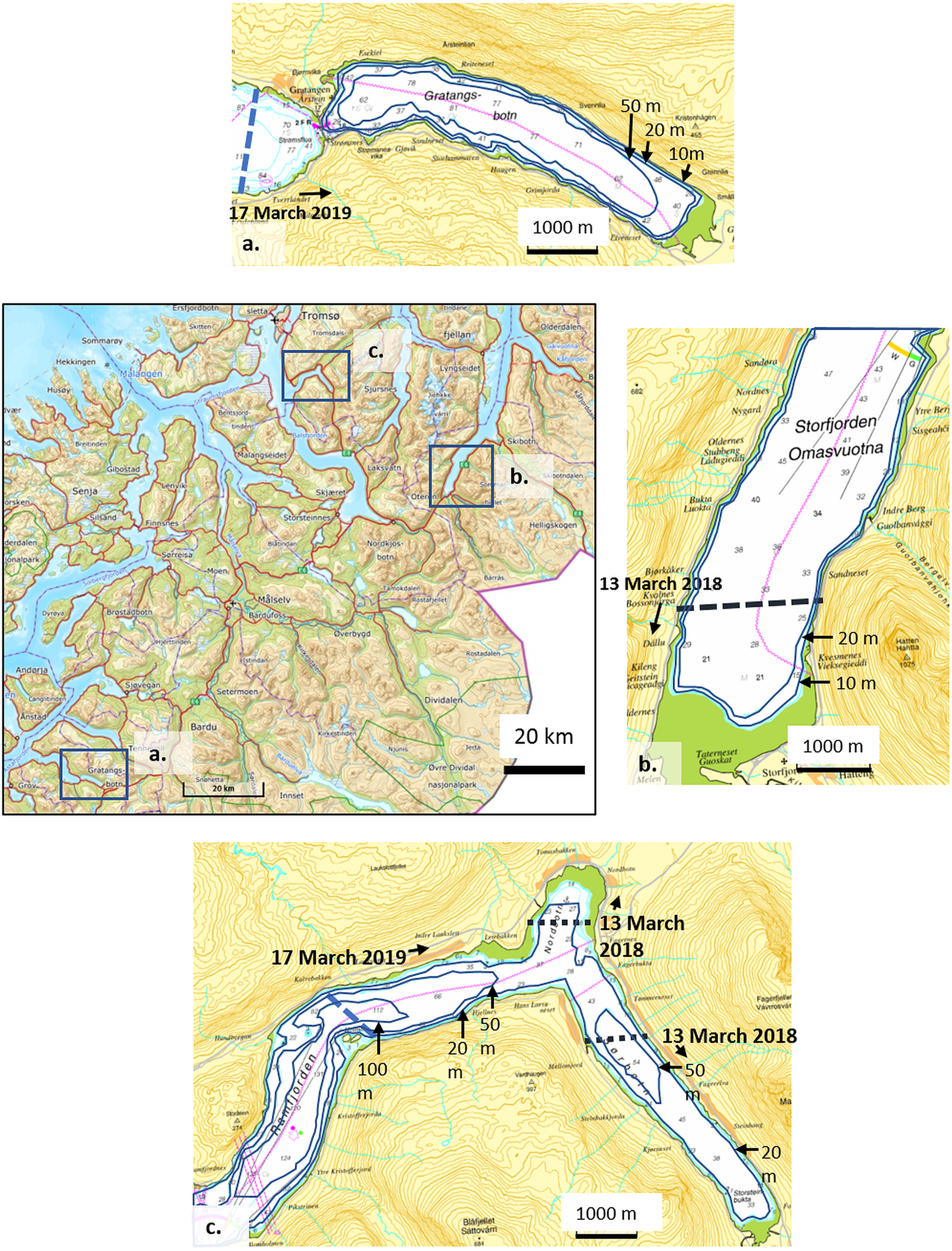
To begin addressing smaller scale, local variations in ice extent, we chose three fjords located within 100 km of each other – Gratangsbotn, Storfjord and Sørbotn/Ramfjord, each located in the Harstad–Skjervøy region (i) (Fig. 1). The shape of each fjord offers an example of the variety one can expect when examining these regions closer (Fig. 9). Gratangsbotn (Fig. 9a) has a fairly consistent width of ~1 km except at its mouth where the fjord narrows to 300 m and the depth decreases to <10 m. Sørbotn/Ramfjord (Fig. 9c), while also having a consistent width between 800 m and 1 km, has a distinct nearly 90° turn with variations in depth throughout. Storfjord (Fig. 9b) is wider being 1.5–2 km in width where ice is known to form. The fjord is substantially longer, extending nearly 75 km, widening and breaking off into other smaller fjords along the way.
Region where the three fjords discussed further are found with each separate fjord boxed and presented on a smaller scale. (a) Gratangsbotn (only ice in 2019), (b) Storfjord (only ice in 2018), (c) Sørbotn/Ramfjord. Ice extent in 2018 and 2019 for each fjord marked with a long-dash black line and short-dash blue line, respectively, and arrows pointing in direction of ice. Fjord bathymetry and depth also marked.
Ice extent for the three fjords since 2001 is presented in Figure 10. Each fjord differs in seasonal and annual variations in ice extent. In Gratangsbotn, years of low ice extent are separated by peaks where ice is present often over a period of time upwards of 2 months in length (Fig. 10a). During the years with ice, the maximum ice extent reached is relatively consistent with >0.50 of the maximum (2010) reached in five separate years. Storfjord showed fewer years of similar ice extent (Fig. 10b), with years of very little or no ice separated by years with none or short-lived ice. In 2018 however, ice was observed throughout the season. Sørbotn/Ramfjord (Fig. 10c) has the most constant ice extent between all years reaching ice extents often above 0.70 of the maximum. Ice was observed every year in Sørbotn/Ramfjord although in 2016 ice extent did not reach above 0.2 of the maximum.
Total ice extent in three fjords for dates 2 February through 24 May, 2001 through 2019 normalized by the maximum ice area measured during this time period. (a) Gratangsbotn, (b) Storfjord, (c) Sørbotn/Ramfjord.

Comparing between fjords during specific years, differing behavior is apparent despite each being located near to each other. For instance, in 2018, Storfjord held ice from approximately 26 February to 14 April, with an abrupt break around 21 March likely due to cloud coverage. Conversely at Gratangsbotn, 2018 was a year with no to little ice, while in Sørbotn/Ramfjord, ice extent stayed below 0.4 the maximum until later in the season. In 2019 however, Storfjord had less consistent ice coverage while Gratangsbotn and Ramfjord/Sørbotn experienced the opposite.
3.4.2 Correlation to weather variables
Out of the three fjords examined individually, only Gratangsbotn showed a significant, albeit moderate, positive correlation – ice extent filtered using only QA data and snowfall (Fig. 11, Table 3). Sørbotn/Ramfjord showed a moderate positive correlation but of less significance between ice extent when filtered using QA/StateQA data and FDD. These findings are therefore partially in alignment with the Harstad–Skjervøy (Table 2) region where all three are located, which had a moderate positive correlation of lower significance to temperature for QA/StateQA filtered ice extent. Snowfall does not appear to have played a dominant role when examining the region as a whole.
Normalized ice extent filtered using QA and StateQA data compared to (a) freezing degree days, (b) sum of daily rainfall plus snowmelt and (c) sum of daily new snowfall for Gratangsbotn, Storfjord and Sørbotn/Ramfjord (marked as Ramfjord). A linear trend line for each region is included to highlight the relationship between and spread of data points.

Correlation and associated p-value between ice extent for each fjord of focus versus the three weather variables discussed

Significant correlations (p < 0.05) marked in gray.
4. Discussion
4.1 Connecting ice conditions to weather events
Through comparison of FDD to measurements of ice thickness, Anderson (Reference Anderson1961) derived a relationship between these two variables to provide an accurate estimation of ice thickness knowing only FDD. Although ice extent, not ice thickness, is considered here, FDD provides a method to examine ice formation based purely on the transfer of heat between air and water. Past studies have used this measurement to look at trends in ice conditions and their possible connection to other variables such as the presence of marine and terrestrial organisms (Petrich and others, Reference Petrich, Tivy and Ward2014). In fjords where FDD is not found to be correlated to ice extent, other factors may be playing a more dominant role in ice formation. The influence of temperature appears to be most prominent in the southern regions of Oslo–Kristiansand (a), Kristiansand–Stavanger (b) and Stavanger–Bergen (c). Moving north, this relationship is less consistent being significant (using both filtering methods) in one region located midway up the coast, Vik–Bodø (f) as well as the most northern region, Skjervøy–Kirkenes (j) using QA/StateQA filtering.
Snowfall and rainfall plus snowmelt have similarities in their potential impact on ice formation through supplying fresh water to a fjord's surface. Rainfall plus snowmelt may not contribute substantially to creating a freshwater layer when applied directly to the surface of a fjord. What likely has a larger impact is the accumulation of rain and snowmelt in rivers and streams leading into a fjord, which can create a freshwater plume and a stratified water column closer to river outlets (Ingram and others, Reference Ingram, Wang, Lin, Legendre and Fortier1996; Granskog and others, Reference Granskog, Ehn and Niemelä2005). Snowfall while not leading to a thick layer of fresh water may assist in ice formation through further cooling the surface and enabling ice formation through seeding the ice. The initial enabling formation of a thin ice layer is capable of dampening small waves allowing for further ice formation (Martin and Kauffman, Reference Martin and Kauffman1981). In addition, once a thin ice layer is created, it allows for accumulation of more snow on top, thickening and strengthening the ice to better withstand fluctuations in weather conditions. If snowfall occurs after a cohesive ice cover has formed however, this snow may alternatively slow ice formation, insulating the ice from the top and allowing more melt from below. Deeper investigation is required to assess which of the two processes, snowfall on the fjord surface versus rainfall plus snowmelt flowing into the fjord, triggers ice formation more efficiently. The mechanism for ice formation, potentially different in southern versus northern fjords, may also lead to differences in ice properties, a topic discussed more below.
The timing of both snowfall and rainfall plus snowmelt events to colder weather likely explains much of the variance in ice extent observed between years and fjords. While a thin ice layer may be able to form a number of times throughout the season, it is vulnerable to break-up given waves, tides or variations in air and water temperature. For ice to stay in place depends on the thickness, or primarily its ability to withstand changing conditions.
It is through examining specific fjords that the unique conditions needed in different regions and even fjords become more apparent. The lack of significant correlations to the three weather variables examined except Gratangsbotn's relation to snowfall illustrates the absence of a general formula combining an input of fresh water, cold weather and their respective timing. Instead, other factors impact ice formation significantly, potentially unique to individual fjords.
4.2 Additional factors to consider
4.2.1 Other weather and oceanic conditions
While several weather variables are considered here, one important factor remaining is wind. Wind provides mixing energy that may act to prevent a cooler, fresher layer of water from forming ice (Manak and Mysak, Reference Manak and Mysak1989). Additionally, any thin ice that may be formed during a calmer period is at risk if and when wind may increase, creating waves to break-up or push ice to another area. Wind strength and direction is difficult to obtain in each individual fjord given the impact of topography which can act to shelter a fjord or conversely to funnel wind to alter predicted wind patterns. Weather models used to predict wind are often produced at resolutions too large for many of the fjords examined. In situ measurements are also limited. The impact of wind on ice conditions in fjords is an important topic that should not be overlooked when analyzing variations in ice conditions in fjords through time. The lack of a significant correlation between ice extent and the variables examined in the regions of Ålesund–Vik (e), Narvik–Lofoten–Harstad (h) and Harstad–Skjervøy (i) and additionally Bodø–Narvik (g) and Skjervøy–Kirkenes (j) when both filtering methods are considered alludes to the influence of other factors, wind likely being one. In future studies, this is recommended to be examined more closely.
Another factor that may lead to mixing and disruption of the stratification that can enable ice formation is tides. Measurements of water temperature in the upper 6 m of the water column in a northern Norwegian fjord known to have ice cover show fluctuations in water temperature aligned with tidal cycles (O'Sadnick and others, Reference O'Sadnick2018). Tides bring in ocean water that may also be of a different salinity, potential mixing and sweeping away layers of fresh or brackish water formed due to water runoff. They also can influence the presence of currents in a fjord (Stigebrandt, Reference Stigebrandt1980; Stigebrandt and Aure, Reference Stigebrandt and Aure1989) which may also impact mixing at varying depths in the water column. Modeling currents within a specific fjord is not simple due to the interaction of current with bed topography and features in the coastline. Understanding the movement of water within a fjord however is useful in determining ocean temperature and related oceanic heat flux, how it may change throughout a day, month or year and if it has potential to control ice extent.
4.2.2 Fjord geometry and bathymetry
Gratangsbotn, Sørbotn/Ramfjord and Storfjord offer an example of the diversity in fjord shape one can encounter within a region. Gratangsbotn has a distinct narrowing where a shallow sill is present. In addition, its shape and bed resemble a bathtub with depth increasing quickly a short distance from the coastline, consistent around its rim (Fig. 6). It is the only fjord out of the three that was significantly correlated to any variable examined, that being snowfall. Additionally, Gratangsbotn displayed large differences in ice extent from year to year, with ice either being non-existent or extending throughout the entirety of the fjord.
The lack of distinct features in the bed or coastline likely contributes to the consistent ice cover when it is present. This is in comparison to Sørbotn/Ramfjord where ice extent appears related to the sharp turn in its coastline as well as areas of varying water depth throughout its length. Ice extent may also be tied to the location of input and amount of fresh water entering a fjord by way of streams and rivers. In Sørbotn/Ramfjord, ice appears to form at the head of the fjord where two rivers enter. Gratangsbotn only has one main river, which itself is smaller than in many other rivers leading into fjords in the area. Given that Gratangsbotn often has a similar ice extent and also a significant correlation to snowfall, one can surmise that the river may not influence ice coverage to the same degree as in other locations like Sørbotn/Ramfjord.
Storfjord displays often the opposite behavior of Gratangsbotn (Figs 10a and b), having greater ice extent in years where Gratangsbotn has lesser or none. The fjord geometry and bathymetry of Storfjord lack abrupt changes in the coastline and ocean bed where ice is present but is considerably wider than the other two examined here, 2 km versus nearer to 1 km. When ice is present, it only extends at most a maximum of 4 km outwards despite a much longer fjord (Fig. 9b). This may be a result of currents and wind on a fjord that due to its width and length, offers less protection against the elements. The last year with substantial ice formation occurred in the winter of 2018, a notably cold and dry season. If conditions were comparatively calm with little wind and resultantly mixing, congelation ice formation due purely to cooling of the ocean from the surface downward may have been possible. Given the lack of a correlation to FDD however, it may be the relationship to another factor such as wind that played the more important role. In comparison, in a fjord such as Gratangsbotn, temperature and FDD may also not be the most important factor but rather a trigger for ice formation, i.e. snowfall just before calm conditions that allow for a strong, cohesive ice cover to form.
Through examining differences in ice extent from year to year between fjords located near to each other, our understanding of how certain factors combine to allow for ice formation can be improved. Fjords displaying similar patterns in ice extent can also be of interest however as the factors contributing may not be the same. For example, both a cold, calm year with little precipitation to form a brackish layer may display the same ice extent as a year with more precipitation but with strong winds in the days directly following. Each fjord may have a different combination of factors leading to variations in ice conditions. For each fjord or region, the questions become:
(1) What factors initiate ice formation?
(2) What factors support an increase in ice extent?
(3) What factors lead to break-up of the initial ice cover, both thin or of substantial thickness?
Understanding historically where ice is present and how it has changed between years in relation to weather and oceanic conditions, as well as its own geometry and bathymetry, helps to identify these factors.
4.3 Implications
Grouping together fjords into regions as done here allows for a first-order analysis of the factors that may be most important when examining trends in sea-ice cover. In future work, focus may be placed more on specific fjords to determine what variables contribute most to sea-ice formation and why, determining if patterns exist between fjords that show stronger correlations to such factors as FDD, snowfall or rainfall/snowmelt. Knowing what factors, and combinations of factors, are most likely to lead to ice formation in each region or fjord allows also for understanding of the properties of the ice such as thickness and porosity that are likely to result.
Ice formed primarily from snow accumulating on a layer of slush or thin ice which turns into a cohesive cover as sea water floods the surface and refreezes is termed granular ice. Such ice typically has a high porosity with pores being connected in all directions through meandering networks of channels. High porosity enables fractures to propagate more easily; this is ideal for boats looking to break through an ice cover but may cause a safety risk if traveling across (Timco and Frederking, Reference Timco and Frederking1982). Once it is emplaced on top of the ocean's surface however, granular ice cover can enable and quicken the growth of congelation ice downward due to its dampening effect on waves. This process requires temperatures cold enough to counteract oceanic heat flux, the latter possibly varying between years. Congelation ice forms directly from the source water, that being either seawater or fresh water. It occurs under quiescent conditions, allowing for slow growth favoring large ice crystals. If fresh water is the source, this ice will be the lowest in porosity, appearing nearly transparent with only air bubbles throughout. In ice formed from saltwater, porosity is higher, the result of salt being rejected from the ice crystal matrix. The pores are connected particularly in the vertical dimension and have a predictable structure based on the temperature of the ice (Petrich and Eicken, Reference Petrich, Eicken, Thomas and Dieckmann2010). The failure mechanisms differ for sea ice versus freshwater ice, the former deforming before breaking thus allowing for some animals or even humans to walk across if they have the correct technique. For all ice types, temperature will largely influence its strength (Assur, Reference Assur1960).
Ice permeability, an indicator of pore connectivity, is also an important characteristic to consider when investigating how ice may interact with the surrounding environment. Given fewer pores in freshwater congelation ice, there is a lack of habitat for marine microbiota. Freshwater ice also does not offer favorable conditions for under-ice algae to grow, a potential source of nutrients for marine life during the winter and initiator of phytoplankton blooms in the summer when ice melts (Granskog and others, Reference Granskog, Kaartokallio and Shirasawa2003; Kaartokallio and others, Reference Kaartokallio, Kuosa, Thomas, Granskog and Kivi2007). In sea ice, a connected pore space provides microbiota a pathway to move upward into the ice where they are protected from predators and can subsist on nutrients in the high salinity brine. Relatedly, algae can be found at the ice–ocean interface in the highly porous skeletal layer (Arrigo and others, Reference Arrigo, Mock, Lizotte, Thomas and Dieckmann2010).
Permeability also determines how a pollutant, such as oil, may pass through the ice. Given a cover of congelation sea ice, oil has the potential to migrate up through the volume, pooling eventually on the surface allowing for cleanup. In freshwater ice, oil does not have a pathway to the surface and therefore can remain under or entrapped in the ice until warmer conditions allow for break-up (Oggier and others, Reference Oggier, Eicken, Petrich, Wilkinson and O'Sadnick2019). These two types of ice, although similar in many aspects in the way they may impact transit through and across, may therefore have a big impact on how one would respond in the case of an oil spill cleanup.
Due to variations in weather and oceanic conditions throughout one season, ice has the possibility to fall between the categories described above – in terms of microstructure and related physical properties. Through considering the factors that ice formation in specific regions or fjords is correlated to, hypotheses can begin to be made in terms of resultant ice conditions. To determine the relation between the factors examined here (i.e. weather, fjord geometry, bed topography), further work must be done. This includes in situ ice sampling of ice properties and the analysis of remote-sensing datasets sensitive to microstructural differences at least in the upper layers of the ice (Hallikainen, Reference Hallikainen and Carsey1994; Tucker and others, Reference Tucker, Perovich, Gow, Weeks, Drinkwater and Carsey1994). Unpredictable and inconsistent ice conditions present a very real risk in an Arctic where traffic is increasing. Therefore, ice conditions both in Norwegian fjords and regions with similar characteristics such as the coast of Greenland or northern Canada where fjords are numerous are an important topic of study.
5. Conclusions
The coast of Norway offers a natural laboratory to explore how differing weather, oceanic conditions, bathymetry and coastal geometry may influence ice extent, conditions and properties important for the safety of the community, those working in these regions, and the environment as a whole. From the work presented here, the following conclusions can be drawn.
– No statistically significant trend in ice extent was found when individual fjords/coastal areas were grouped into regions and total maximum ice extent analyzed between 2001 and 2019.
– Of the 386 fjords and coastal areas chosen, 47 held >5 km2 at least once between 2001 and 2019.
– FDD, a simple measurement of how cold a winter may be in relation to potential ice growth, was significantly correlated to six out of ten regions studied. Additionally, cumulative new snowfall was significantly correlated to ice extent in two regions, and rainfall plus snowfall in one region.
– Seasonal patterns in ice cover are apparent in each region with those lying in the south appearing to break-up and reform while a more consistent ice cover is present in northern regions. The mechanisms of ice formation may influence ice properties, namely ice porosity which will determine ice strength, backscatter signal and permeability.
– The potential impact of unpredictable ice extent and ice properties on boat traffic, local communities, marine life and oil spill cleanup efforts should be considered in future studies. It is recommended to expand the analysis to incorporate more in situ measurements of ice and weather conditions, the latter including wind. Additionally, other regions of the Arctic where fjords are prevalent including northern Canada and Greenland should be examined under a similar lens to determine if similarities exist.
Acknowledgements
This work is funded by the Centre for Integrated Remote Sensing and Forecasting for Arctic Operations (CIRFA), a Centre for Research-based Innovation (Research Council of Norway project number 237906). In addition, we thank the two anonymous reviewers whose constructive feedback greatly added to the presentation and text of the final paper.


 Open access