

1 Introduction
Recent progress in laser technology has led to a dramatic increase of laser power and intensity. The lasers are capable of producing electromagnetic field intensities well above
 $10^{18}~\text{W}~\text{cm}^{-2}$
, which corresponds to the relativistic quiver electron energy, and in the near future their radiation may reach intensities of
$10^{18}~\text{W}~\text{cm}^{-2}$
, which corresponds to the relativistic quiver electron energy, and in the near future their radiation may reach intensities of
 $10^{24}~\text{W}~\text{cm}^{-2}$
and higher (Mourou et al.
Reference Mourou, Korn, Sandner and Collier2011). As a result, the laser–matter interaction will happen in the radiation friction dominated regimes (Marklund & Shukla Reference Marklund and Shukla2006; Mourou, Tajima & Bulanov Reference Mourou, Tajima and Bulanov2006; Di Piazza et al.
Reference Di Piazza, Muller, Hatsagortsyan and Keitel2012). In a strong electromagnetic field, electrons can be accelerated to such high velocities that the radiation reaction starts to play an important role (Zel’dovich Reference Zel’dovich1975; Zhidkov et al.
Reference Zhidkov, Koga, Sasaki and Uesaka2002; Bulanov et al.
Reference Bulanov, Esirkepov, Koga and Tajima2004b
; Di Piazza Reference Di Piazza2008; Harvey, Heinzl & Marklund Reference Harvey, Heinzl and Marklund2011; Thomas et al.
Reference Thomas, Ridgers, Bulanov, Griffin and Mangles2012; Heinzl et al.
Reference Heinzl, Harvey, Ilderton, Marklund, Bulanov, Rykovanov, Schroeder, Esarey and Leemans2015). The radiation friction effects change drastically the laser–plasma interaction leading to fast energy losses (see Koga Reference Koga2004; Koga, Esirkepov & Bulanov Reference Koga, Esirkepov and Bulanov2005, Reference Koga, Esirkepov and Bulanov2006) and to phase space contraction, as discussed in Tamburini et al. (Reference Tamburini, Pegoraro, Di Piazza, Keitel, Liseykina and Macchi2011). Moreover, previously unexplored regimes of the interaction will be entered into, in which quantum electrodynamics (QED) effects such as vacuum polarization, pair production and cascade development can occur (Bell & Kirk Reference Bell and Kirk2008; Di Piazza et al.
Reference Di Piazza, Muller, Hatsagortsyan and Keitel2012).
$10^{24}~\text{W}~\text{cm}^{-2}$
and higher (Mourou et al.
Reference Mourou, Korn, Sandner and Collier2011). As a result, the laser–matter interaction will happen in the radiation friction dominated regimes (Marklund & Shukla Reference Marklund and Shukla2006; Mourou, Tajima & Bulanov Reference Mourou, Tajima and Bulanov2006; Di Piazza et al.
Reference Di Piazza, Muller, Hatsagortsyan and Keitel2012). In a strong electromagnetic field, electrons can be accelerated to such high velocities that the radiation reaction starts to play an important role (Zel’dovich Reference Zel’dovich1975; Zhidkov et al.
Reference Zhidkov, Koga, Sasaki and Uesaka2002; Bulanov et al.
Reference Bulanov, Esirkepov, Koga and Tajima2004b
; Di Piazza Reference Di Piazza2008; Harvey, Heinzl & Marklund Reference Harvey, Heinzl and Marklund2011; Thomas et al.
Reference Thomas, Ridgers, Bulanov, Griffin and Mangles2012; Heinzl et al.
Reference Heinzl, Harvey, Ilderton, Marklund, Bulanov, Rykovanov, Schroeder, Esarey and Leemans2015). The radiation friction effects change drastically the laser–plasma interaction leading to fast energy losses (see Koga Reference Koga2004; Koga, Esirkepov & Bulanov Reference Koga, Esirkepov and Bulanov2005, Reference Koga, Esirkepov and Bulanov2006) and to phase space contraction, as discussed in Tamburini et al. (Reference Tamburini, Pegoraro, Di Piazza, Keitel, Liseykina and Macchi2011). Moreover, previously unexplored regimes of the interaction will be entered into, in which quantum electrodynamics (QED) effects such as vacuum polarization, pair production and cascade development can occur (Bell & Kirk Reference Bell and Kirk2008; Di Piazza et al.
Reference Di Piazza, Muller, Hatsagortsyan and Keitel2012).
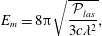
An electromagnetic field intensity of the order of
 $10^{24}~\text{W}~\text{cm}^{-2}$
can be achieved in the focus of a
$10^{24}~\text{W}~\text{cm}^{-2}$
can be achieved in the focus of a
 $1~\unicode[STIX]{x03BC}\text{m}$
wavelength laser of ten petawatt power. For 30 fs, i.e. for a ten wave period duration, the laser pulse energy is approximately 300 J. Within the framework of the multiple colliding laser pulses (MCLP) concept formulated in Bulanov et al. (Reference Bulanov, Mur, Narozhny, Nees and Popov2010b
) (see Bulanov et al. (Reference Bulanov, Esirkepov, Koga, Thomas and Bulanov2010a
), Gonoskov et al. (Reference Gonoskov, Aiello, Heugel and Leuchs2012, Reference Gonoskov, Gonoskov, Harvey, Ilderton, Kim, Marklund, Mourou and Sergeev2013), Gelfer et al. (Reference Gelfer, Mironov, Fedotov, Bashmakov, Nerush, Kostyukov and Narozhny2015) for development of this idea), the laser radiation with given energy
$1~\unicode[STIX]{x03BC}\text{m}$
wavelength laser of ten petawatt power. For 30 fs, i.e. for a ten wave period duration, the laser pulse energy is approximately 300 J. Within the framework of the multiple colliding laser pulses (MCLP) concept formulated in Bulanov et al. (Reference Bulanov, Mur, Narozhny, Nees and Popov2010b
) (see Bulanov et al. (Reference Bulanov, Esirkepov, Koga, Thomas and Bulanov2010a
), Gonoskov et al. (Reference Gonoskov, Aiello, Heugel and Leuchs2012, Reference Gonoskov, Gonoskov, Harvey, Ilderton, Kim, Marklund, Mourou and Sergeev2013), Gelfer et al. (Reference Gelfer, Mironov, Fedotov, Bashmakov, Nerush, Kostyukov and Narozhny2015) for development of this idea), the laser radiation with given energy
 ${\mathcal{E}}_{las}$
is subdivided into several beams each of them having
${\mathcal{E}}_{las}$
is subdivided into several beams each of them having
 $1/N$
of the laser energy, where
$1/N$
of the laser energy, where
 $N$
is the number of beams. If the beams interfere in the focus in a constructive way, i.e. their electric fields are summed, the resulting electric field and the laser intensity are equal to
$N$
is the number of beams. If the beams interfere in the focus in a constructive way, i.e. their electric fields are summed, the resulting electric field and the laser intensity are equal to
 $E_{N}=\sqrt{N}E_{las}$
and
$E_{N}=\sqrt{N}E_{las}$
and
 $I_{N}=NI_{las}$
, respectively. Here
$I_{N}=NI_{las}$
, respectively. Here
 $E_{las}$
and
$E_{las}$
and
 $I_{las}$
are the electric field and the intensity of the laser light. For a large number of beams there is a diffraction constraint on the electric field amplitude in the focus region. In the limit
$I_{las}$
are the electric field and the intensity of the laser light. For a large number of beams there is a diffraction constraint on the electric field amplitude in the focus region. In the limit
 $N\rightarrow \infty$
the electromagnetic field can be approximated by the three-dimensional dipole configurations (see Bulanov et al.
Reference Bulanov, Esirkepov, Koga, Thomas and Bulanov2010a
) for which the electric field maximum is given by (Bassett Reference Bassett1986)
$N\rightarrow \infty$
the electromagnetic field can be approximated by the three-dimensional dipole configurations (see Bulanov et al.
Reference Bulanov, Esirkepov, Koga, Thomas and Bulanov2010a
) for which the electric field maximum is given by (Bassett Reference Bassett1986)
 $$\begin{eqnarray}E_{m}=8\unicode[STIX]{x03C0}\sqrt{\frac{{\mathcal{P}}_{las}}{3c\unicode[STIX]{x1D706}^{2}}},\end{eqnarray}$$
where
 ${\mathcal{P}}_{las}$
,
${\mathcal{P}}_{las}$
,
 $\unicode[STIX]{x1D706}$
and
$\unicode[STIX]{x1D706}$
and
 $c$
are the laser power, wavelength and speed of light in vacuum, respectively.
$c$
are the laser power, wavelength and speed of light in vacuum, respectively.
Since the radiation friction and QED processes both depend on the particle’s momentum, the strength of the present electromagnetic field and on their mutual orientation, they are crucial in understanding the dynamics of charged particles in an electromagnetic field in the regime of radiation dominance. Even in the simplest MCLP case, two counter-propagating plane waves, the particle behaviour in the standing wave is quite complicated. It demonstrates regular and chaotic motion, random walk, limit circles and strange attractors as is shown by Mendonca (Reference Mendonca1983), Bauer, Mulser & Steeb (Reference Bauer, Mulser and Steeb1995), Sheng et al. (Reference Sheng, Mima, Sentoku, Jovanovic, Taguchi, Zhang and Meyer-ter Vehn2002), Lehmann & Spatschek (Reference Lehmann and Spatschek2012, Reference Lehmann and Spatschek2016), Gonoskov et al. (Reference Gonoskov, Bashinov, Gonoskov, Harvey, Ilderton, Kim, Marklund, Mourou and Sergeev2014), Bashinov, Kim & Sergeev (Reference Bashinov, Kim and Sergeev2015), Bulanov et al. (Reference Bulanov, Esirkepov, Kando, Koga, Kondo and Korn2015), Esirkepov et al. (Reference Esirkepov, Bulanov, Koga, Kando, Kondo, Rosanov, Korn and Bulanov2015), Jirka et al. (Reference Jirka, Klimo, Bulanov, Esirkepov, Gelfer, Bulanov, Weber and Korn2016), Kirk (Reference Kirk2016). As is well known, the standing wave configuration is widely used in classical electrodynamics and in QED theory. This is due to the fact that in the planes where the magnetic field vanishes, the charged particle may be considered to be interacting with an oscillating pure electric field. This provides great simplification of the theoretical description. In addition, as has been noted above, in a standing wave formed by two colliding laser pulses, the resulting electromagnetic (EM) field configuration facilitates QED effects (see Bulanov et al.
Reference Bulanov, Narozhny, Mur and Popov2004a
, Reference Bulanov, Narozhny, Mur and Popov2006, Reference Bulanov, Mur, Narozhny, Nees and Popov2010b
). Computer simulations presented in Gonoskov et al. (Reference Gonoskov, Bashinov, Bastrakov, Efimenko, Ilderton, Kim, Marklund, Meyerov, Muraviev and Sergeev2016), Gong et al. (Reference Gong, Hu, Shou, Qiao, Chen, He, Bulanov, Esirkepov, Bulanov and Yan2017), Vranic et al. (Reference Vranic, Grismayer, Fonseca and Silva2017) show that the MCLP concept can be beneficial for realizing such important laser–matter interaction regimes as, for example, the electron–positron pair production via the Breit–Wheeler process (see Vranic et al.
Reference Vranic, Grismayer, Fonseca and Silva2017) and the high efficiency
 $\unicode[STIX]{x1D6FE}$
-ray flash generation due to nonlinear Thomson or multi-photon Compton scattering, as shown in Gonoskov et al. (Reference Gonoskov, Bashinov, Bastrakov, Efimenko, Ilderton, Kim, Marklund, Meyerov, Muraviev and Sergeev2016), Gong et al. (Reference Gong, Hu, Shou, Qiao, Chen, He, Bulanov, Esirkepov, Bulanov and Yan2017). Another configuration for the generation of a
$\unicode[STIX]{x1D6FE}$
-ray flash generation due to nonlinear Thomson or multi-photon Compton scattering, as shown in Gonoskov et al. (Reference Gonoskov, Bashinov, Bastrakov, Efimenko, Ilderton, Kim, Marklund, Meyerov, Muraviev and Sergeev2016), Gong et al. (Reference Gong, Hu, Shou, Qiao, Chen, He, Bulanov, Esirkepov, Bulanov and Yan2017). Another configuration for the generation of a
 $\unicode[STIX]{x1D6FE}$
-ray flash is a single laser pulse irradiating an overdense plasma target (see Nakamura et al.
Reference Nakamura, Koga, Esirkepov, Kando, Korn and Bulanov2012; Ridgers et al.
Reference Ridgers, Brady, Duclous, Kirk, Bennett, Arber, Robinson and Bell2012; Corvan, Zepf & Sarri Reference Corvan, Zepf and Sarri2016; Levy et al.
Reference Levy, Blackburn, Ratan, Sadler, Ridgers, Kasim, Ceurvorst, Holloway, Baring and Bell2016). The applications of the laser based
$\unicode[STIX]{x1D6FE}$
-ray flash is a single laser pulse irradiating an overdense plasma target (see Nakamura et al.
Reference Nakamura, Koga, Esirkepov, Kando, Korn and Bulanov2012; Ridgers et al.
Reference Ridgers, Brady, Duclous, Kirk, Bennett, Arber, Robinson and Bell2012; Corvan, Zepf & Sarri Reference Corvan, Zepf and Sarri2016; Levy et al.
Reference Levy, Blackburn, Ratan, Sadler, Ridgers, Kasim, Ceurvorst, Holloway, Baring and Bell2016). The applications of the laser based
 $\unicode[STIX]{x1D6FE}$
-ray sources are reviewed in Gales et al. (Reference Gales, Balabanski, Negoita, Tesileanu, Ur, Ursescu and Zamfir2016). The radiation friction effects on ion acceleration, on magnetic field self-generation and on high-order harmonics in laser plasmas have been studied in Tamburini et al. (Reference Tamburini, Pegoraro, Di Piazza, Keitel and Macchi2010, Reference Tamburini, Pegoraro, Di Piazza, Keitel, Liseykina and Macchi2011), Liseykina, Popruzhenko & Macchi (Reference Liseykina, Popruzhenko and Macchi2016) and Tang, Kumar & Keitel (Reference Tang, Kumar and Keitel2016), respectively.
$\unicode[STIX]{x1D6FE}$
-ray sources are reviewed in Gales et al. (Reference Gales, Balabanski, Negoita, Tesileanu, Ur, Ursescu and Zamfir2016). The radiation friction effects on ion acceleration, on magnetic field self-generation and on high-order harmonics in laser plasmas have been studied in Tamburini et al. (Reference Tamburini, Pegoraro, Di Piazza, Keitel and Macchi2010, Reference Tamburini, Pegoraro, Di Piazza, Keitel, Liseykina and Macchi2011), Liseykina, Popruzhenko & Macchi (Reference Liseykina, Popruzhenko and Macchi2016) and Tang, Kumar & Keitel (Reference Tang, Kumar and Keitel2016), respectively.
It is not surprising that the dynamics of the electron interacting with three-, four-, etc. colliding pulses is even more complicated and rich with novel patterns.
The present paper contains the theoretical analysis of the electron motion in the standing EM wave generated by two, three and four colliding focused EM pulses. The paper is organized as follows. In the next section we introduce the notations used, describe the field configurations and equations of motion and present the dimensionless parameters characterizing the charged particle interaction with a high intensity EM field. Then, in § 3 we briefly recover the main features of the electron motion in two counter-propagating plane waves. In § 4 we formulate a simple theoretical model of the stabilization of the particle motion in the oscillating field due to nonlinear dissipation effects, which explains the radiative electron trapping revealed earlier in Gonoskov et al. (Reference Gonoskov, Aiello, Heugel and Leuchs2012, Reference Gonoskov, Gonoskov, Harvey, Ilderton, Kim, Marklund, Mourou and Sergeev2013), Ji et al. (Reference Ji, Pukhov, Kostyukov, Shen and Akli2014), Bulanov et al. (Reference Bulanov, Esirkepov, Kando, Koga, Kondo and Korn2015), Esirkepov et al. (Reference Esirkepov, Bulanov, Koga, Kando, Kondo, Rosanov, Korn and Bulanov2015), Jirka et al. (Reference Jirka, Klimo, Bulanov, Esirkepov, Gelfer, Bulanov, Weber and Korn2016), Kirk (Reference Kirk2016). Section 5 relates to the regular and chaotic electron motion in three s-polarized laser pulses. The radiating electron dynamics in the four s- and p-polarized colliding EM pulses is discussed in § 6. Section 7 summarizes the conclusions.
2 Field configurations, dimensionless parameters and equations of motion
2.1
 $N$
colliding EM waves
$N$
colliding EM waves

Consider
 $N$
monochromatic plane waves in vacuum with the same frequencies
$N$
monochromatic plane waves in vacuum with the same frequencies
 $\unicode[STIX]{x1D714}_{0}$
and equal amplitudes
$\unicode[STIX]{x1D714}_{0}$
and equal amplitudes
 $a_{n}$
. We assume that the wave vectors
$a_{n}$
. We assume that the wave vectors
 $\boldsymbol{k}_{n}$
are in the
$\boldsymbol{k}_{n}$
are in the
 $(x,y)$
plane. The wave vector of the
$(x,y)$
plane. The wave vector of the
 $n_{th}$
wave is equal to
$n_{th}$
wave is equal to
 $$\begin{eqnarray}\boldsymbol{k}_{n}=k_{0}[\sin (\unicode[STIX]{x1D703}_{n})\boldsymbol{e}_{x}+\cos (\unicode[STIX]{x1D703}_{n})\boldsymbol{e}_{y}],\end{eqnarray}$$
where
 $k_{0}=\unicode[STIX]{x1D714}_{0}/c$
,
$k_{0}=\unicode[STIX]{x1D714}_{0}/c$
,
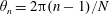 $\unicode[STIX]{x1D703}_{n}=2\unicode[STIX]{x03C0}(n-1)/N$
,
$\unicode[STIX]{x1D703}_{n}=2\unicode[STIX]{x03C0}(n-1)/N$
,
 $n=1,2,3,\ldots ,N$
and
$n=1,2,3,\ldots ,N$
and
 $\boldsymbol{e}_{x}$
and
$\boldsymbol{e}_{x}$
and
 $\boldsymbol{e}_{y}$
are unit vectors in the
$\boldsymbol{e}_{y}$
are unit vectors in the
 $x$
and
$x$
and
 $y$
directions.
$y$
directions.
It is convenient to describe the s-polarized EM waves with the electric field normal to the
 $(x,y)$
plane, i.e.
$(x,y)$
plane, i.e.
 $\boldsymbol{E}=E_{z}\boldsymbol{e}_{z}$
with the unit vector
$\boldsymbol{E}=E_{z}\boldsymbol{e}_{z}$
with the unit vector
 $\boldsymbol{e}_{z}$
along the
$\boldsymbol{e}_{z}$
along the
 $z$
direction, in terms of
$z$
direction, in terms of
 $E_{z}(x,y,t)$
equal to
$E_{z}(x,y,t)$
equal to
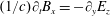
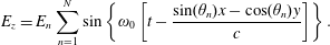 $$\begin{eqnarray}E_{z}=E_{n}\mathop{\sum }_{n=1}^{N}\sin \left\{\unicode[STIX]{x1D714}_{0}\left[t-\frac{\sin (\unicode[STIX]{x1D703}_{n})x-\cos (\unicode[STIX]{x1D703}_{n})y}{c}\right]\right\}.\end{eqnarray}$$
Here the amplitude of the
 $n_{th}$
wave is
$n_{th}$
wave is
 $E_{n}=E_{0}/\sqrt{N}$
where
$E_{n}=E_{0}/\sqrt{N}$
where
 $E_{0}=E_{las}$
. The magnetic field can be expressed by using Maxwell’s equations:
$E_{0}=E_{las}$
. The magnetic field can be expressed by using Maxwell’s equations:
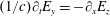
 $(1/c)\unicode[STIX]{x2202}_{t}B_{x}=-\unicode[STIX]{x2202}_{y}E_{z}$
and
$(1/c)\unicode[STIX]{x2202}_{t}B_{x}=-\unicode[STIX]{x2202}_{y}E_{z}$
and
 $(1/c)\unicode[STIX]{x2202}_{t}B_{y}=\unicode[STIX]{x2202}_{x}E_{z}$
.
$(1/c)\unicode[STIX]{x2202}_{t}B_{y}=\unicode[STIX]{x2202}_{x}E_{z}$
.
In the case of p-polarized EM waves with the magnetic field normal to the
 $(x,y)$
plane,
$(x,y)$
plane,
 $\boldsymbol{B}=B_{z}\boldsymbol{e}_{z}$
, the
$\boldsymbol{B}=B_{z}\boldsymbol{e}_{z}$
, the
 $B_{z}$
field of colliding
$B_{z}$
field of colliding
 $N$
pules is given by
$N$
pules is given by
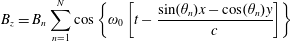 $$\begin{eqnarray}B_{z}=B_{n}\mathop{\sum }_{n=1}^{N}\cos \left\{\unicode[STIX]{x1D714}_{0}\left[t-\frac{\sin (\unicode[STIX]{x1D703}_{n})x-\cos (\unicode[STIX]{x1D703}_{n})y}{c}\right]\right\}\end{eqnarray}$$
with
 $B_{n}=E_{las}/\sqrt{N}$
and the electric field components expressed via Maxwell’s equations as
$B_{n}=E_{las}/\sqrt{N}$
and the electric field components expressed via Maxwell’s equations as
 $(1/c)\unicode[STIX]{x2202}_{t}E_{x}=\unicode[STIX]{x2202}_{y}B_{z}$
and
$(1/c)\unicode[STIX]{x2202}_{t}E_{x}=\unicode[STIX]{x2202}_{y}B_{z}$
and
 $(1/c)\unicode[STIX]{x2202}_{t}E_{y}=-\unicode[STIX]{x2202}_{x}E_{z}$
, respectively.
$(1/c)\unicode[STIX]{x2202}_{t}E_{y}=-\unicode[STIX]{x2202}_{x}E_{z}$
, respectively.
2.2 Dimensionless parameters characterizing interaction of laser radiation with charged particles
Introducing the normalized variables, we change the space and time coordinates to
 $x/\unicode[STIX]{x1D706}\rightarrow x$
and
$x/\unicode[STIX]{x1D706}\rightarrow x$
and
 $t\unicode[STIX]{x1D714}/2\unicode[STIX]{x03C0}\rightarrow t$
.
$t\unicode[STIX]{x1D714}/2\unicode[STIX]{x03C0}\rightarrow t$
.
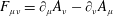
The interaction of charged particles with intense EM fields is characterized by several dimensionless and relativistic invariant parameters (Nikishov & Ritus Reference Nikishov and Ritus1964a ; Di Piazza et al. Reference Di Piazza, Muller, Hatsagortsyan and Keitel2012; Bulanov et al. Reference Bulanov, Esirkepov, Kando, Koga, Kondo and Korn2015).
The first parameter is
 $$\begin{eqnarray}a=\frac{e\sqrt{A_{\unicode[STIX]{x1D707}}A^{\unicode[STIX]{x1D707}}}}{m_{e}c^{2}},\end{eqnarray}$$
where
 $A^{\unicode[STIX]{x1D707}}$
is the 4-potential of the electromagnetic field with
$A^{\unicode[STIX]{x1D707}}$
is the 4-potential of the electromagnetic field with
 $\unicode[STIX]{x1D707}=0,1,2,3,4$
. Here and below summation over repeating indexes is assumed. This parameter is relativistically invariant for a plane EM wave. It is related to the wave normalized amplitude introduced above. When it is equal to unity, i.e. the intensity of a linearly polarized EM wave is
$\unicode[STIX]{x1D707}=0,1,2,3,4$
. Here and below summation over repeating indexes is assumed. This parameter is relativistically invariant for a plane EM wave. It is related to the wave normalized amplitude introduced above. When it is equal to unity, i.e. the intensity of a linearly polarized EM wave is
 $I_{R}=1.37\times 10^{18}(1~\unicode[STIX]{x03BC}\text{m}/\unicode[STIX]{x1D706})^{2}~\text{W}~\text{cm}^{-2}$
, the quiver electron motion becomes relativistic.
$I_{R}=1.37\times 10^{18}(1~\unicode[STIX]{x03BC}\text{m}/\unicode[STIX]{x1D706})^{2}~\text{W}~\text{cm}^{-2}$
, the quiver electron motion becomes relativistic.
The ratio,
 $eE/m_{e}\unicode[STIX]{x1D714}c$
, the dimensionless EM field amplitude, measures the work in units of
$eE/m_{e}\unicode[STIX]{x1D714}c$
, the dimensionless EM field amplitude, measures the work in units of
 $m_{e}c^{2}$
produced by the field on an electron over the distance equal to the field wavelength. Here,
$m_{e}c^{2}$
produced by the field on an electron over the distance equal to the field wavelength. Here,
 $e$
and
$e$
and
 $m_{e}$
are the charge and mass of an electron,
$m_{e}$
are the charge and mass of an electron,
 $E$
and
$E$
and
 $\unicode[STIX]{x1D714}$
are the EM field strength and frequency and
$\unicode[STIX]{x1D714}$
are the EM field strength and frequency and
 $c$
is the speed of light.
$c$
is the speed of light.
The second dimensionless parameter is
 $\unicode[STIX]{x1D700}_{rad}$
:
$\unicode[STIX]{x1D700}_{rad}$
:
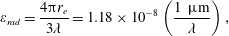 $$\begin{eqnarray}\unicode[STIX]{x1D700}_{rad}=\frac{4\unicode[STIX]{x03C0}r_{e}}{3\unicode[STIX]{x1D706}}=1.18\times 10^{-8}\left(\frac{1~\unicode[STIX]{x03BC}\text{m}}{\unicode[STIX]{x1D706}}\right),\end{eqnarray}$$
which is proportional to the ratio of the classical electron radius
 $r_{e}=e^{2}/m_{e}c^{2}=2.8\times 10^{-13}$
cm to the laser radiation wavelength,
$r_{e}=e^{2}/m_{e}c^{2}=2.8\times 10^{-13}$
cm to the laser radiation wavelength,
 $\unicode[STIX]{x1D706}$
. It essentially determines the strength of the radiation reaction effects for an electron radiating an EM wave.
$\unicode[STIX]{x1D706}$
. It essentially determines the strength of the radiation reaction effects for an electron radiating an EM wave.
When one micron wavelength laser intensities exceed
 $10^{23}~\text{W}~\text{cm}^{-2}$
, the nonlinear quantum electrodynamics effects begin to play a significant role in laser plasma interactions (e.g. see Bulanov et al. (Reference Bulanov, Esirkepov, Kando, Koga, Kondo and Korn2015) and literature cited therein). These effects manifest themselves through multi-photon Compton and Breit–Wheeler effects (Nikishov & Ritus Reference Nikishov and Ritus1964a
,Reference Nikishov and Ritus
b
; Ritus Reference Ritus1985) (see Narozhnyi & Fofanov (Reference Narozhnyi and Fofanov1996), Boca & Florescu (Reference Boca and Florescu2009), Ehlotzky, Krajewska & Kamiśki (Reference Ehlotzky, Krajewska and Kamiśki2009), Heinzl, Ilderton & Marklund (Reference Heinzl, Ilderton and Marklund2010a
), Heinzl, Seipt & Kämpfer (Reference Heinzl, Seipt and Kämpfer2010b
), Mackenroth & Di Piazza (Reference Mackenroth and Di Piazza2011), Krajewska & Kamiński (Reference Krajewska and Kamiński2012), Titov et al. (Reference Titov, Takabe, Kämpfer and Hosaka2012), Harvey, Heinzl & Ilderton (Reference Harvey, Heinzl and Ilderton2009) for recent studies), i.e. through either photon emission by an electron or positron, or electron–positron pair production by a high energy photon, respectively. The multi-photon Compton and Breit–Wheeler processes are characterized in terms of two dimensionless relativistic and gauge invariant parameters (Nikishov & Ritus Reference Nikishov and Ritus1964a
):
$10^{23}~\text{W}~\text{cm}^{-2}$
, the nonlinear quantum electrodynamics effects begin to play a significant role in laser plasma interactions (e.g. see Bulanov et al. (Reference Bulanov, Esirkepov, Kando, Koga, Kondo and Korn2015) and literature cited therein). These effects manifest themselves through multi-photon Compton and Breit–Wheeler effects (Nikishov & Ritus Reference Nikishov and Ritus1964a
,Reference Nikishov and Ritus
b
; Ritus Reference Ritus1985) (see Narozhnyi & Fofanov (Reference Narozhnyi and Fofanov1996), Boca & Florescu (Reference Boca and Florescu2009), Ehlotzky, Krajewska & Kamiśki (Reference Ehlotzky, Krajewska and Kamiśki2009), Heinzl, Ilderton & Marklund (Reference Heinzl, Ilderton and Marklund2010a
), Heinzl, Seipt & Kämpfer (Reference Heinzl, Seipt and Kämpfer2010b
), Mackenroth & Di Piazza (Reference Mackenroth and Di Piazza2011), Krajewska & Kamiński (Reference Krajewska and Kamiński2012), Titov et al. (Reference Titov, Takabe, Kämpfer and Hosaka2012), Harvey, Heinzl & Ilderton (Reference Harvey, Heinzl and Ilderton2009) for recent studies), i.e. through either photon emission by an electron or positron, or electron–positron pair production by a high energy photon, respectively. The multi-photon Compton and Breit–Wheeler processes are characterized in terms of two dimensionless relativistic and gauge invariant parameters (Nikishov & Ritus Reference Nikishov and Ritus1964a
):
 $$\begin{eqnarray}\unicode[STIX]{x1D712}_{e}=\frac{\sqrt{|F^{\unicode[STIX]{x1D707}\unicode[STIX]{x1D708}}p_{\unicode[STIX]{x1D708}}|^{2}}}{E_{S}m_{e}c}\quad \text{and}\quad \unicode[STIX]{x1D712}_{\unicode[STIX]{x1D6FE}}=\frac{\unicode[STIX]{x1D706}_{C}\sqrt{|F^{\unicode[STIX]{x1D707}\unicode[STIX]{x1D708}}k_{\unicode[STIX]{x1D708}}|^{2}}}{E_{S}}.\end{eqnarray}$$
where
 $p_{\unicode[STIX]{x1D708}}$
and
$p_{\unicode[STIX]{x1D708}}$
and
 $\hbar k_{\unicode[STIX]{x1D708}}$
denote the 4-momenta of an electron or positron undergoing the Compton process and a photon undergoing the Breit–Wheeler process, the 4-tensor of the electromagnetic field is defined as
$\hbar k_{\unicode[STIX]{x1D708}}$
denote the 4-momenta of an electron or positron undergoing the Compton process and a photon undergoing the Breit–Wheeler process, the 4-tensor of the electromagnetic field is defined as
 $F_{\unicode[STIX]{x1D707}\unicode[STIX]{x1D708}}=\unicode[STIX]{x2202}_{\unicode[STIX]{x1D707}}A_{\unicode[STIX]{x1D708}}-\unicode[STIX]{x2202}_{\unicode[STIX]{x1D708}}A_{\unicode[STIX]{x1D707}}$
, with the critical QED electric field
$F_{\unicode[STIX]{x1D707}\unicode[STIX]{x1D708}}=\unicode[STIX]{x2202}_{\unicode[STIX]{x1D707}}A_{\unicode[STIX]{x1D708}}-\unicode[STIX]{x2202}_{\unicode[STIX]{x1D708}}A_{\unicode[STIX]{x1D707}}$
, with the critical QED electric field
 $$\begin{eqnarray}E_{S}=\frac{m_{e}^{2}c^{3}}{e\hbar }.\end{eqnarray}$$
This field is also known as the ‘Schwinger field’ (Beresteskii, Lifshitz & Pitaevskii Reference Beresteskii, Lifshitz and Pitaevskii1982). Its amplitude is approximately
 $10^{18}~\text{V}~\text{cm}^{-1}$
, which corresponds to the radiation intensity
$10^{18}~\text{V}~\text{cm}^{-1}$
, which corresponds to the radiation intensity
 ${\approx}10^{29}~\text{W}~\text{cm}^{-2}$
. The work produced by the field
${\approx}10^{29}~\text{W}~\text{cm}^{-2}$
. The work produced by the field
 $E_{S}$
on an electron over the distance equal to the reduced Compton wavelength,
$E_{S}$
on an electron over the distance equal to the reduced Compton wavelength,
 $\unicode[STIX]{x1D706}_{C}=\hbar /m_{e}c=3.86\times 10^{-11}~\text{cm}$
equals
$\unicode[STIX]{x1D706}_{C}=\hbar /m_{e}c=3.86\times 10^{-11}~\text{cm}$
equals
 $m_{e}c^{2}$
. Here
$m_{e}c^{2}$
. Here
 $\hbar$
is the reduced Planck constant.
$\hbar$
is the reduced Planck constant.
In three-dimensional (3-D) notation the parameter
 $\unicode[STIX]{x1D712}_{e}$
given by (2.6) reads
$\unicode[STIX]{x1D712}_{e}$
given by (2.6) reads
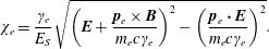 $$\begin{eqnarray}\unicode[STIX]{x1D712}_{e}=\frac{\unicode[STIX]{x1D6FE}_{e}}{E_{S}}\sqrt{\left(\boldsymbol{E}+\frac{\boldsymbol{ p}_{e}\times \boldsymbol{ B}}{m_{e}c\unicode[STIX]{x1D6FE}_{e}}\right)^{2}-\left(\frac{\boldsymbol{p}_{e}\boldsymbol{\cdot }\boldsymbol{E}}{m_{e}c\unicode[STIX]{x1D6FE}_{e}}\right)^{2}}.\end{eqnarray}$$
For the parameter
 $\unicode[STIX]{x1D712}_{\unicode[STIX]{x1D6FE}}$
defined by (2.6) we have
$\unicode[STIX]{x1D712}_{\unicode[STIX]{x1D6FE}}$
defined by (2.6) we have
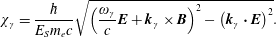 $$\begin{eqnarray}\unicode[STIX]{x1D712}_{\unicode[STIX]{x1D6FE}}=\frac{\hbar }{E_{S}m_{e}c}\sqrt{\left(\frac{\unicode[STIX]{x1D714}_{\unicode[STIX]{x1D6FE}}}{c}\boldsymbol{E}+\boldsymbol{k}_{\unicode[STIX]{x1D6FE}}\times \boldsymbol{B}\right)^{2}-\left(\boldsymbol{k}_{\unicode[STIX]{x1D6FE}}\boldsymbol{\cdot }\boldsymbol{E}\right)^{2}}.\end{eqnarray}$$
Here
 $\unicode[STIX]{x1D6FE}_{e}$
,
$\unicode[STIX]{x1D6FE}_{e}$
,
 $\boldsymbol{p}_{e}$
,
$\boldsymbol{p}_{e}$
,
 $\unicode[STIX]{x1D714}_{\unicode[STIX]{x1D6FE}}$
and
$\unicode[STIX]{x1D714}_{\unicode[STIX]{x1D6FE}}$
and
 $\boldsymbol{k}_{\unicode[STIX]{x1D6FE}}$
correspond to the representation of the electron 4-momentum
$\boldsymbol{k}_{\unicode[STIX]{x1D6FE}}$
correspond to the representation of the electron 4-momentum
 $p_{\unicode[STIX]{x1D708}}$
and of the photon 4-wavenumber
$p_{\unicode[STIX]{x1D708}}$
and of the photon 4-wavenumber
 $k_{\unicode[STIX]{x1D708}}$
as
$k_{\unicode[STIX]{x1D708}}$
as
 $p_{\unicode[STIX]{x1D708}}=(\unicode[STIX]{x1D6FE}_{e}m_{e}c,\boldsymbol{p})$
and
$p_{\unicode[STIX]{x1D708}}=(\unicode[STIX]{x1D6FE}_{e}m_{e}c,\boldsymbol{p})$
and
 $k_{\unicode[STIX]{x1D708}}=(\unicode[STIX]{x1D714}_{\unicode[STIX]{x1D6FE}}/c,\boldsymbol{k}_{\unicode[STIX]{x1D6FE}})$
, respectively. The parameter
$k_{\unicode[STIX]{x1D708}}=(\unicode[STIX]{x1D714}_{\unicode[STIX]{x1D6FE}}/c,\boldsymbol{k}_{\unicode[STIX]{x1D6FE}})$
, respectively. The parameter
 $\unicode[STIX]{x1D712}_{e}$
can also be defined as the ratio of the electric field to the critical electric field of quantum electrodynamics,
$\unicode[STIX]{x1D712}_{e}$
can also be defined as the ratio of the electric field to the critical electric field of quantum electrodynamics,
 $E_{S}$
, in the electron rest frame. In particular, it characterizes the probability of the gamma–photon emission by an electron with 4-momentum
$E_{S}$
, in the electron rest frame. In particular, it characterizes the probability of the gamma–photon emission by an electron with 4-momentum
 $p_{\unicode[STIX]{x1D708}}$
in the field of the electromagnetic wave, in the Compton scattering process.
$p_{\unicode[STIX]{x1D708}}$
in the field of the electromagnetic wave, in the Compton scattering process.
The parameter
 $\unicode[STIX]{x1D712}_{\unicode[STIX]{x1D6FE}}$
characterizes the probability of electron–positron pair creation by the photon with the momentum
$\unicode[STIX]{x1D712}_{\unicode[STIX]{x1D6FE}}$
characterizes the probability of electron–positron pair creation by the photon with the momentum
 $\hbar k_{\unicode[STIX]{x1D708}}$
interacting with a strong EM wave in the Breit–Wheeler process.
$\hbar k_{\unicode[STIX]{x1D708}}$
interacting with a strong EM wave in the Breit–Wheeler process.
The probabilities of the Compton scattering and of the Breit–Wheeler processes depend strongly on
 $\unicode[STIX]{x1D712}_{e}$
and
$\unicode[STIX]{x1D712}_{e}$
and
 $\unicode[STIX]{x1D712}_{\unicode[STIX]{x1D6FE}}$
, reaching optimal values when
$\unicode[STIX]{x1D712}_{\unicode[STIX]{x1D6FE}}$
, reaching optimal values when
 $\unicode[STIX]{x1D712}_{e}\sim 1$
and
$\unicode[STIX]{x1D712}_{e}\sim 1$
and
 $\unicode[STIX]{x1D712}_{\unicode[STIX]{x1D6FE}}\sim 1$
(Nikishov & Ritus Reference Nikishov and Ritus1964a
).
$\unicode[STIX]{x1D712}_{\unicode[STIX]{x1D6FE}}\sim 1$
(Nikishov & Ritus Reference Nikishov and Ritus1964a
).
In the case of an electron interaction with a plane EM wave propagating along the
 $x$
-axis with phase and group velocity equal to speed of light in vacuum the parameters of the interaction can be written in terms of EM field strength, normalized by the QED critical field given by (2.7), and either the electron
$x$
-axis with phase and group velocity equal to speed of light in vacuum the parameters of the interaction can be written in terms of EM field strength, normalized by the QED critical field given by (2.7), and either the electron
 $\unicode[STIX]{x1D6FE}_{e}$
-factor or the photon energy
$\unicode[STIX]{x1D6FE}_{e}$
-factor or the photon energy
 $\hbar \unicode[STIX]{x1D714}_{\unicode[STIX]{x1D6FE}}$
:
$\hbar \unicode[STIX]{x1D714}_{\unicode[STIX]{x1D6FE}}$
:
 $$\begin{eqnarray}\unicode[STIX]{x1D712}_{e}=\frac{E}{E_{S}}\left(\unicode[STIX]{x1D6FE}_{e}-\frac{p_{x}}{m_{e}c}\right)\end{eqnarray}$$
and
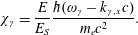 $$\begin{eqnarray}\unicode[STIX]{x1D712}_{\unicode[STIX]{x1D6FE}}=\frac{E}{E_{S}}\frac{\hbar (\unicode[STIX]{x1D714}_{\unicode[STIX]{x1D6FE}}-k_{\unicode[STIX]{x1D6FE},x}c)}{m_{e}c^{2}}.\end{eqnarray}$$
For an electron interacting with the EM wave the linear combination of the electron energy and momentum,
 $$\begin{eqnarray}h_{e}=\unicode[STIX]{x1D6FE}_{e}-p_{x}/m_{e}c,\end{eqnarray}$$
on the right-hand side of (2.10) is an integral of motion (Landau & Lifshitz Reference Landau and Lifshitz1982). Its value is determined by initial conditions.
If an electron/positron or a photon co-propagates with the EM wave, then in the former case the parameter
 $\unicode[STIX]{x1D712}_{e}$
is suppressed by a factor
$\unicode[STIX]{x1D712}_{e}$
is suppressed by a factor
 $(2\unicode[STIX]{x1D6FE}_{e,0})^{-1}$
, i.e.
$(2\unicode[STIX]{x1D6FE}_{e,0})^{-1}$
, i.e.
 $\unicode[STIX]{x1D712}_{e}\simeq (2\unicode[STIX]{x1D6FE}_{e,0})^{-1}(E/E_{S})$
, where
$\unicode[STIX]{x1D712}_{e}\simeq (2\unicode[STIX]{x1D6FE}_{e,0})^{-1}(E/E_{S})$
, where
 $\unicode[STIX]{x1D6FE}_{e,0}$
is the electron gamma-factor before interaction with the laser pulse. In the later case, when the gamma–photon co-propagates with the EM wave, the parameter
$\unicode[STIX]{x1D6FE}_{e,0}$
is the electron gamma-factor before interaction with the laser pulse. In the later case, when the gamma–photon co-propagates with the EM wave, the parameter
 $\unicode[STIX]{x1D712}_{\unicode[STIX]{x1D6FE}}$
is equal to zero,
$\unicode[STIX]{x1D712}_{\unicode[STIX]{x1D6FE}}$
is equal to zero,
 $\unicode[STIX]{x1D712}_{\unicode[STIX]{x1D6FE}}=0$
, because
$\unicode[STIX]{x1D712}_{\unicode[STIX]{x1D6FE}}=0$
, because
 $\unicode[STIX]{x1D714}_{\unicode[STIX]{x1D6FE}}=k_{\unicode[STIX]{x1D6FE},x}c$
. On the contrary, the parameter
$\unicode[STIX]{x1D714}_{\unicode[STIX]{x1D6FE}}=k_{\unicode[STIX]{x1D6FE},x}c$
. On the contrary, the parameter
 $\unicode[STIX]{x1D712}_{e}$
can be enhanced to approximately
$\unicode[STIX]{x1D712}_{e}$
can be enhanced to approximately
 $2\unicode[STIX]{x1D6FE}_{e,0}E/E_{S}$
, when the electron interacts with a counter-propagating laser pulse. Therefore the head-on collision configuration has an apparent advantage for strengthening the electron–EM wave interaction and, in particular, for enhancing the
$2\unicode[STIX]{x1D6FE}_{e,0}E/E_{S}$
, when the electron interacts with a counter-propagating laser pulse. Therefore the head-on collision configuration has an apparent advantage for strengthening the electron–EM wave interaction and, in particular, for enhancing the
 $\unicode[STIX]{x1D6FE}$
-ray production due to nonlinear Thomson or/and Compton scattering.
$\unicode[STIX]{x1D6FE}$
-ray production due to nonlinear Thomson or/and Compton scattering.
Depending on the energy of charged particles and field strength the interaction happens in one of the following regimes parametrized by the values of
 $a$
,
$a$
,
 $\unicode[STIX]{x1D712}_{e}$
and
$\unicode[STIX]{x1D712}_{e}$
and
 $\unicode[STIX]{x1D712}_{\unicode[STIX]{x1D6FE}}$
:
$\unicode[STIX]{x1D712}_{\unicode[STIX]{x1D6FE}}$
:
-
(i)
$a>1$
, the relativistic interaction regime (Mourou et al.
Reference Mourou, Tajima and Bulanov2006); -
(ii)
$a>\unicode[STIX]{x1D700}_{rad}^{-1/3}$
, the interaction becomes radiation dominated (Zhidkov et al.
Reference Zhidkov, Koga, Sasaki and Uesaka2002; Bulanov et al.
Reference Bulanov, Esirkepov, Koga and Tajima2004b
; Bashinov & Kim Reference Bashinov and Kim2013); -
(iii)
$\unicode[STIX]{x1D712}_{e}\geqslant 1$
the quantum effects begin to manifest themselves (Di Piazza, Hatsagortsyan & Keitel Reference Di Piazza, Hatsagortsyan and Keitel2010; Bulanov et al.
Reference Bulanov, Esirkepov, Hayashi, Kando, Kiriyama, Koga, Kondo, Kotaki, Pirozhkov and Bulanov2011a
, Reference Bulanov, Esirkepov, Kando, Koga, Kondo and Korn2015); and -
(iv)
$\unicode[STIX]{x1D712}_{e}>1$
,
$\unicode[STIX]{x1D712}_{\unicode[STIX]{x1D6FE}}>1$
marks the condition for the EM avalanche (Bulanov et al.
Reference Bulanov, Esirkepov, Koga, Thomas and Bulanov2010a
; Fedotov et al.
Reference Fedotov, Narozhny, Mourou and Korn2010; Elkina et al.
Reference Elkina, Fedotov, Kostyukov, Legkov, Narozhny, Nerush and Ruhl2011; Nerush et al.
Reference Nerush, Kostyukov, Fedotov, Narozhny, Elkina and Ruhl2011; Bulanov et al.
Reference Bulanov, Schroeder, Esarey and Leemans2013), which is the phenomenon of exponential growth of the number of electron–positrons and photons in the strong EM field, being able to develop. These conditions can be supplemented by
$\unicode[STIX]{x1D6FC}a>1$
, which indicates that the number of photons emitted incoherently per laser period can be larger than unity as has been noted by Di Piazza et al. (Reference Di Piazza, Hatsagortsyan and Keitel2010). Here the parameter
$\unicode[STIX]{x1D700}_{rad}$
is given by (2.5) and
$\unicode[STIX]{x1D6FC}=e^{2}/\hbar c\approx 1/137$
is the fine structure constant.


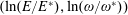
Regimes of electromagnetic field interaction with matter on the plane of parameters: (a) the normalized EM wave amplitude
 $a\unicode[STIX]{x1D700}_{rad}^{1/3}$
and the parameter
$a\unicode[STIX]{x1D700}_{rad}^{1/3}$
and the parameter
 $\unicode[STIX]{x1D712}_{e}$
; (b) accordingly the
$\unicode[STIX]{x1D712}_{e}$
; (b) accordingly the
 $(\ln (E/E^{\ast }),\ln (\unicode[STIX]{x1D714}/\unicode[STIX]{x1D714}^{\ast }))$
plane, where
$(\ln (E/E^{\ast }),\ln (\unicode[STIX]{x1D714}/\unicode[STIX]{x1D714}^{\ast }))$
plane, where
 $E^{\ast }$
and
$E^{\ast }$
and
 $\unicode[STIX]{x1D714}^{\ast }$
are given by (2.14) and (2.15), respectively. The parameter planes are subdivided into 4 domains: (I) electron – EM field interaction in the particle dominated radiation reaction domain; (II) electron – EM field interaction is dominated by the radiation reaction; (III) electron – EM field interaction is in the particle dominated QED regime; (IV) electron – EM field interaction is in the radiation dominated QED regime.
$\unicode[STIX]{x1D714}^{\ast }$
are given by (2.14) and (2.15), respectively. The parameter planes are subdivided into 4 domains: (I) electron – EM field interaction in the particle dominated radiation reaction domain; (II) electron – EM field interaction is dominated by the radiation reaction; (III) electron – EM field interaction is in the particle dominated QED regime; (IV) electron – EM field interaction is in the radiation dominated QED regime.
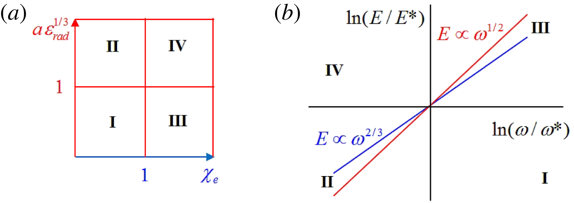
As one can see two dimensionless parameters,
 $a$
and
$a$
and
 $\unicode[STIX]{x1D712}_{e}$
, can be used to subdivide the
$\unicode[STIX]{x1D712}_{e}$
, can be used to subdivide the
 $(a,\unicode[STIX]{x1D712}_{e})$
plane into four domains shown in figure 1(a) (see also Bulanov et al.
Reference Bulanov, Esirkepov, Kando, Koga, Kondo and Korn2015; Bulanov Reference Bulanov2017). The
$(a,\unicode[STIX]{x1D712}_{e})$
plane into four domains shown in figure 1(a) (see also Bulanov et al.
Reference Bulanov, Esirkepov, Kando, Koga, Kondo and Korn2015; Bulanov Reference Bulanov2017). The
 $\unicode[STIX]{x1D712}_{e}=1$
line divides the plane into the radiation reaction description of the interaction domain (
$\unicode[STIX]{x1D712}_{e}=1$
line divides the plane into the radiation reaction description of the interaction domain (
 $\unicode[STIX]{x1D712}_{e}<1$
) and QED description of interaction domain (
$\unicode[STIX]{x1D712}_{e}<1$
) and QED description of interaction domain (
 $\unicode[STIX]{x1D712}_{e}>1$
). The
$\unicode[STIX]{x1D712}_{e}>1$
). The
 $a=\unicode[STIX]{x1D700}_{rad}^{-1/3}$
line divides the plane into radiation dominated (
$a=\unicode[STIX]{x1D700}_{rad}^{-1/3}$
line divides the plane into radiation dominated (
 $a>\unicode[STIX]{x1D700}_{rad}^{-1/3}$
) and particle dominated (
$a>\unicode[STIX]{x1D700}_{rad}^{-1/3}$
) and particle dominated (
 $a<\unicode[STIX]{x1D700}_{rad}^{-1/3}$
) regimes of interaction domains. We note that the
$a<\unicode[STIX]{x1D700}_{rad}^{-1/3}$
) regimes of interaction domains. We note that the
 $a=\unicode[STIX]{x1D700}_{rad}^{-1/3}$
threshold comes from the requirement for an electron to emit the amount of energy per EM wave period equal to the energy gain from the EM wave during the wave period. If one takes into account the discrete nature of the photon emission, then the same condition will take the form
$a=\unicode[STIX]{x1D700}_{rad}^{-1/3}$
threshold comes from the requirement for an electron to emit the amount of energy per EM wave period equal to the energy gain from the EM wave during the wave period. If one takes into account the discrete nature of the photon emission, then the same condition will take the form
 $a\,m_{e}c^{2}=\hbar \unicode[STIX]{x1D714}_{\unicode[STIX]{x1D6FE}}(\unicode[STIX]{x1D706}/L_{R})$
(Ritus Reference Ritus1985), where
$a\,m_{e}c^{2}=\hbar \unicode[STIX]{x1D714}_{\unicode[STIX]{x1D6FE}}(\unicode[STIX]{x1D706}/L_{R})$
(Ritus Reference Ritus1985), where
 $L_{R}$
is the radiation length is of the order of
$L_{R}$
is the radiation length is of the order of
 $2\unicode[STIX]{x1D706}/a$
for
$2\unicode[STIX]{x1D706}/a$
for
 $\unicode[STIX]{x1D712}_{e}\ll 1$
and
$\unicode[STIX]{x1D712}_{e}\ll 1$
and
 $\unicode[STIX]{x1D706}\unicode[STIX]{x1D6FE}_{e}^{1/3}/a^{2/3}$
for
$\unicode[STIX]{x1D706}\unicode[STIX]{x1D6FE}_{e}^{1/3}/a^{2/3}$
for
 $\unicode[STIX]{x1D712}_{e}\gg 1$
(Nikishov & Ritus Reference Nikishov and Ritus1964a
,Reference Nikishov and Ritus
b
; Bolotovskii & Voskresenskii Reference Bolotovskii and Voskresenskii1966; Ritus Reference Ritus1985). This condition in the limit
$\unicode[STIX]{x1D712}_{e}\gg 1$
(Nikishov & Ritus Reference Nikishov and Ritus1964a
,Reference Nikishov and Ritus
b
; Bolotovskii & Voskresenskii Reference Bolotovskii and Voskresenskii1966; Ritus Reference Ritus1985). This condition in the limit
 $\unicode[STIX]{x1D712}_{e}\rightarrow 0$
tends to the classical limit
$\unicode[STIX]{x1D712}_{e}\rightarrow 0$
tends to the classical limit
 $a=\unicode[STIX]{x1D700}_{rad}^{-1/3}$
.
$a=\unicode[STIX]{x1D700}_{rad}^{-1/3}$
.
The intersection point, where
 $a_{rad}=\unicode[STIX]{x1D700}_{rad}^{-1/3}$
and the parameter
$a_{rad}=\unicode[STIX]{x1D700}_{rad}^{-1/3}$
and the parameter
 $\unicode[STIX]{x1D712}_{e}$
is equal to unity, determines critical values of the EM wave amplitude
$\unicode[STIX]{x1D712}_{e}$
is equal to unity, determines critical values of the EM wave amplitude
 $\unicode[STIX]{x1D718}_{a}a^{\ast }$
with
$\unicode[STIX]{x1D718}_{a}a^{\ast }$
with
 $$\begin{eqnarray}a^{\ast }=\left(\frac{3c}{2r_{e}\unicode[STIX]{x1D714}^{\ast }}\right)^{1/3}=\frac{\hbar c}{e^{2}}=\frac{1}{\unicode[STIX]{x1D6FC}},\end{eqnarray}$$
i.e. the wave electric field is
 $\unicode[STIX]{x1D718}_{a}\unicode[STIX]{x1D718}_{\unicode[STIX]{x1D714}}E^{\ast }$
, where
$\unicode[STIX]{x1D718}_{a}\unicode[STIX]{x1D718}_{\unicode[STIX]{x1D714}}E^{\ast }$
, where
 $$\begin{eqnarray}E^{\ast }=E_{S}\unicode[STIX]{x1D6FC},\end{eqnarray}$$
and the wave frequency
 $\unicode[STIX]{x1D718}_{\unicode[STIX]{x1D714}}\unicode[STIX]{x1D714}^{\ast }$
with
$\unicode[STIX]{x1D718}_{\unicode[STIX]{x1D714}}\unicode[STIX]{x1D714}^{\ast }$
with
 $\unicode[STIX]{x1D714}^{\ast }$
given by
$\unicode[STIX]{x1D714}^{\ast }$
given by
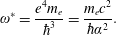 $$\begin{eqnarray}\unicode[STIX]{x1D714}^{\ast }=\frac{e^{4}m_{e}}{\hbar ^{3}}=\frac{m_{e}c^{2}}{\hbar \unicode[STIX]{x1D6FC}^{2}}.\end{eqnarray}$$
Here
 $\unicode[STIX]{x1D6FC}=1/137$
is the fine structure constant and
$\unicode[STIX]{x1D6FC}=1/137$
is the fine structure constant and
 $\unicode[STIX]{x1D718}_{a}$
and
$\unicode[STIX]{x1D718}_{a}$
and
 $\unicode[STIX]{x1D718}_{\unicode[STIX]{x1D714}}$
are constants of the order of unity. The normalized EM wave amplitude equals
$\unicode[STIX]{x1D718}_{\unicode[STIX]{x1D714}}$
are constants of the order of unity. The normalized EM wave amplitude equals
 $a^{\ast }=137$
with corresponding wave intensity
$a^{\ast }=137$
with corresponding wave intensity
 $I^{\ast }=2.6\times 10^{22}~\text{W}~\text{cm}^{-2}$
. The corresponding photon energy is
$I^{\ast }=2.6\times 10^{22}~\text{W}~\text{cm}^{-2}$
. The corresponding photon energy is
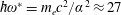 $\hbar \unicode[STIX]{x1D714}^{\ast }=m_{e}c^{2}/\unicode[STIX]{x1D6FC}^{2}\approx 27$
eV. We note that the value of
$\hbar \unicode[STIX]{x1D714}^{\ast }=m_{e}c^{2}/\unicode[STIX]{x1D6FC}^{2}\approx 27$
eV. We note that the value of
 $a^{\ast }=1/\unicode[STIX]{x1D6FC}$
corresponds to one of the conditions for the charged particle interaction with the EM field to be in the QED regime,
$a^{\ast }=1/\unicode[STIX]{x1D6FC}$
corresponds to one of the conditions for the charged particle interaction with the EM field to be in the QED regime,
 $\unicode[STIX]{x1D6FC}a>1$
(see also Di Piazza et al.
Reference Di Piazza, Hatsagortsyan and Keitel2010).
$\unicode[STIX]{x1D6FC}a>1$
(see also Di Piazza et al.
Reference Di Piazza, Hatsagortsyan and Keitel2010).
Concrete values of the coefficients
 $\unicode[STIX]{x1D718}_{a}$
and
$\unicode[STIX]{x1D718}_{a}$
and
 $\unicode[STIX]{x1D718}_{\unicode[STIX]{x1D714}}$
depend on the specific electromagnetic configuration. For example, in the case of a rotating homogeneous electric field (which can be formed in the antinodes of an electric field in the standing EM wave) analysed in Bulanov et al. (Reference Bulanov, Esirkepov, Kando, Koga, Kondo and Korn2015), they are
$\unicode[STIX]{x1D718}_{\unicode[STIX]{x1D714}}$
depend on the specific electromagnetic configuration. For example, in the case of a rotating homogeneous electric field (which can be formed in the antinodes of an electric field in the standing EM wave) analysed in Bulanov et al. (Reference Bulanov, Esirkepov, Kando, Koga, Kondo and Korn2015), they are
 $\unicode[STIX]{x1D718}_{a}=3$
and
$\unicode[STIX]{x1D718}_{a}=3$
and
 $\unicode[STIX]{x1D718}_{\unicode[STIX]{x1D714}}=1/18$
, respectively, which gives
$\unicode[STIX]{x1D718}_{\unicode[STIX]{x1D714}}=1/18$
, respectively, which gives
 $\unicode[STIX]{x1D718}_{a}a^{\ast }=411$
, with the intensity equal to
$\unicode[STIX]{x1D718}_{a}a^{\ast }=411$
, with the intensity equal to
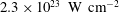 $2.3\times 10^{23}~\text{W}~\text{cm}^{-2}$
, and
$2.3\times 10^{23}~\text{W}~\text{cm}^{-2}$
, and
 $\unicode[STIX]{x1D718}_{\unicode[STIX]{x1D714}}\hbar \unicode[STIX]{x1D714}^{\ast }=m_{e}c^{2}\unicode[STIX]{x1D6FC}^{2}/18\approx 1.5$
eV.
$\unicode[STIX]{x1D718}_{\unicode[STIX]{x1D714}}\hbar \unicode[STIX]{x1D714}^{\ast }=m_{e}c^{2}\unicode[STIX]{x1D6FC}^{2}/18\approx 1.5$
eV.
Here we would like to attract attention to the relationship between the well-known critical electric field of classical electrodynamics
 $E_{cr}$
, the critical electric field of quantum electrodynamics
$E_{cr}$
, the critical electric field of quantum electrodynamics
 $E_{S}$
and the electric field
$E_{S}$
and the electric field
 $E^{\ast }$
. They can be written as
$E^{\ast }$
. They can be written as
 $E_{cr}=e/r_{e}^{2}$
,
$E_{cr}=e/r_{e}^{2}$
,
 $E_{S}=e/r_{e}\unicode[STIX]{x1D706}_{C}$
and
$E_{S}=e/r_{e}\unicode[STIX]{x1D706}_{C}$
and
 $E^{\ast }\approx e/\unicode[STIX]{x1D706}_{C}^{2}$
, respectively. In other words we have
$E^{\ast }\approx e/\unicode[STIX]{x1D706}_{C}^{2}$
, respectively. In other words we have
 $E_{S}=E_{cr}\unicode[STIX]{x1D6FC}$
and
$E_{S}=E_{cr}\unicode[STIX]{x1D6FC}$
and
 $E^{\ast }=E_{cr}\unicode[STIX]{x1D6FC}^{2}$
.
$E^{\ast }=E_{cr}\unicode[STIX]{x1D6FC}^{2}$
.
Using the relationships obtained above we find that on the line
 $a\unicode[STIX]{x1D700}_{rad}^{1/3}=1$
the wave electric field is proportional to the frequency in the
$a\unicode[STIX]{x1D700}_{rad}^{1/3}=1$
the wave electric field is proportional to the frequency in the
 $2/3$
power, i.e.
$2/3$
power, i.e.
 $E/E^{\ast }=(\unicode[STIX]{x1D714}/\unicode[STIX]{x1D714}^{\ast })^{2/3}$
, and on the line
$E/E^{\ast }=(\unicode[STIX]{x1D714}/\unicode[STIX]{x1D714}^{\ast })^{2/3}$
, and on the line
 $\unicode[STIX]{x1D712}_{e}=1$
we have
$\unicode[STIX]{x1D712}_{e}=1$
we have
 $E/E^{\ast }=(\unicode[STIX]{x1D714}/\unicode[STIX]{x1D714}^{\ast })^{1/2}$
.
$E/E^{\ast }=(\unicode[STIX]{x1D714}/\unicode[STIX]{x1D714}^{\ast })^{1/2}$
.
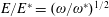
Figure 1(b) shows the
 $(\ln (E/E^{\ast }),\ln (\unicode[STIX]{x1D714}/\unicode[STIX]{x1D714}^{\ast }))$
plane with 4 domains. The lines intersect each other at the point
$(\ln (E/E^{\ast }),\ln (\unicode[STIX]{x1D714}/\unicode[STIX]{x1D714}^{\ast }))$
plane with 4 domains. The lines intersect each other at the point
 $(0,0)$
, i.e. at the point where
$(0,0)$
, i.e. at the point where
 $E=E^{\ast }$
and
$E=E^{\ast }$
and
 $\unicode[STIX]{x1D714}=\unicode[STIX]{x1D714}^{\ast }$
.
$\unicode[STIX]{x1D714}=\unicode[STIX]{x1D714}^{\ast }$
.
2.3 Radiation friction force with the QED form factor
In order to describe the relativistic electron dynamics in the electromagnetic field we shall use the equations of electron motion:
 $$\begin{eqnarray}\displaystyle & \displaystyle \frac{\text{d}\boldsymbol{p}}{\text{d}t}=e\left(\boldsymbol{E}+\frac{\boldsymbol{v}}{c}\times \boldsymbol{B}\right)+F_{rad}, & \displaystyle\end{eqnarray}$$
 $$\begin{eqnarray}\displaystyle & \displaystyle \frac{\text{d}\boldsymbol{x}}{\text{d}t}=\frac{\boldsymbol{p}}{m_{e}\unicode[STIX]{x1D6FE}}, & \displaystyle\end{eqnarray}$$
where the radiation friction force,
 $F_{rad}=G_{e}\boldsymbol{f}_{rad}$
, is the product of the classical radiation friction force,
$F_{rad}=G_{e}\boldsymbol{f}_{rad}$
, is the product of the classical radiation friction force,
 $\boldsymbol{f}_{rad}$
, in the Landau–Lifshitz form (Landau & Lifshitz Reference Landau and Lifshitz1982):
$\boldsymbol{f}_{rad}$
, in the Landau–Lifshitz form (Landau & Lifshitz Reference Landau and Lifshitz1982):
 $$\begin{eqnarray}\displaystyle \boldsymbol{f}_{rad} & = & \displaystyle \frac{2e^{3}}{3m_{e}c^{3}\unicode[STIX]{x1D6FE}}\left\{\unicode[STIX]{x2202}_{t}+(\boldsymbol{v}\unicode[STIX]{x1D735})\boldsymbol{E}+\frac{1}{c}[\boldsymbol{v}\times (\unicode[STIX]{x2202}_{t}+(\boldsymbol{v}\unicode[STIX]{x1D735})\boldsymbol{B}]\right\}\nonumber\\ \displaystyle & & \displaystyle +\,\frac{2e^{4}}{3m_{e}^{2}c^{4}}\left\{\boldsymbol{E}\times \boldsymbol{B}+\frac{1}{c}[\boldsymbol{B}\times (\boldsymbol{B}\times \boldsymbol{v})+\boldsymbol{E}(\boldsymbol{v}\boldsymbol{\cdot }\boldsymbol{E})]\right\}\nonumber\\ \displaystyle & & \displaystyle -\,\frac{2e^{4}}{3m_{e}^{2}c^{5}}\unicode[STIX]{x1D6FE}^{2}\boldsymbol{v}\left\{\left(\boldsymbol{E}+\frac{1}{c}\boldsymbol{v}\times \boldsymbol{B}\right)^{2}-\frac{1}{c^{2}}(\boldsymbol{v}\boldsymbol{\cdot }\boldsymbol{E})^{2}\right\}\end{eqnarray}$$
and a form factor
 $G_{e}$
, which takes into account the quantum electrodynamics weakening of the radiation friction (Sokolov, Klepikov & Ternov Reference Sokolov, Klepikov and Ternov1952; Schwinger Reference Schwinger1954; Erber Reference Erber1966; Beresteskii et al.
Reference Beresteskii, Lifshitz and Pitaevskii1982; Sokolov et al.
Reference Sokolov, Nees, Yanovsky, Naumova and Mourou2010). Discussions of the relationship between the Landau–Lifshitz and Lorentz–Abraham–Dirac forms of the radiation friction force and what form of the force follows from the QED calculation, can be found in Bulanov et al. (Reference Bulanov, Esirkepov, Kando, Koga and Bulanov2011b
), Ilderton & Torgrimsson (Reference Ilderton and Torgrimsson2013), Zhang (Reference Zhang2013) and in the literature cited therein.
$G_{e}$
, which takes into account the quantum electrodynamics weakening of the radiation friction (Sokolov, Klepikov & Ternov Reference Sokolov, Klepikov and Ternov1952; Schwinger Reference Schwinger1954; Erber Reference Erber1966; Beresteskii et al.
Reference Beresteskii, Lifshitz and Pitaevskii1982; Sokolov et al.
Reference Sokolov, Nees, Yanovsky, Naumova and Mourou2010). Discussions of the relationship between the Landau–Lifshitz and Lorentz–Abraham–Dirac forms of the radiation friction force and what form of the force follows from the QED calculation, can be found in Bulanov et al. (Reference Bulanov, Esirkepov, Kando, Koga and Bulanov2011b
), Ilderton & Torgrimsson (Reference Ilderton and Torgrimsson2013), Zhang (Reference Zhang2013) and in the literature cited therein.
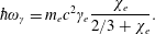
As we have noted above, the threshold of the QED effects is determined by the dimensionless parameter
 $\unicode[STIX]{x1D712}_{e}$
given by (2.8). For example, if an electron moves in the magnetic field
$\unicode[STIX]{x1D712}_{e}$
given by (2.8). For example, if an electron moves in the magnetic field
 $B$
, the parameter is equal to
$B$
, the parameter is equal to
 $\unicode[STIX]{x1D712}_{e}\approx \unicode[STIX]{x1D6FE}_{e}(B/B_{S})$
, where
$\unicode[STIX]{x1D712}_{e}\approx \unicode[STIX]{x1D6FE}_{e}(B/B_{S})$
, where
 $B_{S}=m_{e}^{2}c^{3}/e\hbar$
is the QED critical magnetic field (see also (2.7)). The energy of the emitted synchrotron photons is
$B_{S}=m_{e}^{2}c^{3}/e\hbar$
is the QED critical magnetic field (see also (2.7)). The energy of the emitted synchrotron photons is
 $$\begin{eqnarray}\hbar \unicode[STIX]{x1D714}_{\unicode[STIX]{x1D6FE}}=m_{e}c^{2}\unicode[STIX]{x1D6FE}_{e}\frac{\unicode[STIX]{x1D712}_{e}}{2/3+\unicode[STIX]{x1D712}_{e}}.\end{eqnarray}$$
In the limit
 $\unicode[STIX]{x1D712}_{e}\ll 1$
the frequency
$\unicode[STIX]{x1D712}_{e}\ll 1$
the frequency
 $\unicode[STIX]{x1D714}_{\unicode[STIX]{x1D6FE}}$
is equal to
$\unicode[STIX]{x1D714}_{\unicode[STIX]{x1D6FE}}$
is equal to
 $(3/2)\unicode[STIX]{x1D714}_{Be}\unicode[STIX]{x1D6FE}_{e}^{2}$
in accordance with classical electrodynamics (see Landau & Lifshitz Reference Landau and Lifshitz1982). Here
$(3/2)\unicode[STIX]{x1D714}_{Be}\unicode[STIX]{x1D6FE}_{e}^{2}$
in accordance with classical electrodynamics (see Landau & Lifshitz Reference Landau and Lifshitz1982). Here
 $\unicode[STIX]{x1D714}_{Be}=eB/m_{e}c$
is the Larmor frequency. If
$\unicode[STIX]{x1D714}_{Be}=eB/m_{e}c$
is the Larmor frequency. If
 $\unicode[STIX]{x1D712}_{e}\gg 1$
the photon energy is equal to the energy of the radiating electron:
$\unicode[STIX]{x1D712}_{e}\gg 1$
the photon energy is equal to the energy of the radiating electron:
 $\hbar \unicode[STIX]{x1D714}_{\unicode[STIX]{x1D6FE}}=m_{e}c^{2}\unicode[STIX]{x1D6FE}_{e}$
.
$\hbar \unicode[STIX]{x1D714}_{\unicode[STIX]{x1D6FE}}=m_{e}c^{2}\unicode[STIX]{x1D6FE}_{e}$
.
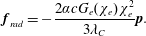
The radiation friction force in the limit
 $\unicode[STIX]{x1D6FE}_{e}\rightarrow \infty$
, i.e. the last term on the right-hand side of (2.18) retained, can be written in the following form (see also Sokolov et al. (Reference Sokolov, Klepikov and Ternov1952), Schwinger (Reference Schwinger1954), Erber (Reference Erber1966), Sokolov et al. (Reference Sokolov, Nees, Yanovsky, Naumova and Mourou2010), Bulanov et al. (Reference Bulanov, Esirkepov, Kando, Koga, Kondo and Korn2015) and literature cited therein)
$\unicode[STIX]{x1D6FE}_{e}\rightarrow \infty$
, i.e. the last term on the right-hand side of (2.18) retained, can be written in the following form (see also Sokolov et al. (Reference Sokolov, Klepikov and Ternov1952), Schwinger (Reference Schwinger1954), Erber (Reference Erber1966), Sokolov et al. (Reference Sokolov, Nees, Yanovsky, Naumova and Mourou2010), Bulanov et al. (Reference Bulanov, Esirkepov, Kando, Koga, Kondo and Korn2015) and literature cited therein)
 $$\begin{eqnarray}\boldsymbol{f}_{rad}=-\frac{2\unicode[STIX]{x1D6FC}cG_{e}(\unicode[STIX]{x1D712}_{e})\unicode[STIX]{x1D712}_{e}^{2}}{3\unicode[STIX]{x1D706}_{C}}\boldsymbol{p}.\end{eqnarray}$$
Here the QED effects are incorporated into the equations of the electron motion by using the form factor
 $G_{e}(\unicode[STIX]{x1D712}_{e})$
(see Sokolov et al.
Reference Sokolov, Klepikov and Ternov1952), which is equal to the ratio of full radiation intensity to the intensity of the radiation emitted by a classical electron. It reads
$G_{e}(\unicode[STIX]{x1D712}_{e})$
(see Sokolov et al.
Reference Sokolov, Klepikov and Ternov1952), which is equal to the ratio of full radiation intensity to the intensity of the radiation emitted by a classical electron. It reads
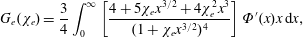 $$\begin{eqnarray}G_{e}(\unicode[STIX]{x1D712}_{e})=\frac{3}{4}\int _{0}^{\infty }\left[\frac{4+5\unicode[STIX]{x1D712}_{e}x^{3/2}+4\unicode[STIX]{x1D712}_{e}^{2}x^{3}}{(1+\unicode[STIX]{x1D712}_{e}x^{3/2})^{4}}\right]\unicode[STIX]{x1D6F7}^{\prime }(x)x\,\text{d}x,\end{eqnarray}$$
where
 $\unicode[STIX]{x1D6F7}(x)$
is the Airy function (Abramovitz & Stegun Reference Abramovitz and Stegun1964). In (2.20) we neglect the effects of the discrete nature of the photon emission in quantum electrodynamics (see Duclous, Kirk & Bell Reference Duclous, Kirk and Bell2011; Brady et al.
Reference Brady, Ridgers, Arber, Bell and Kirk2012; Thomas et al.
Reference Thomas, Ridgers, Bulanov, Griffin and Mangles2012; Bulanov et al.
Reference Bulanov, Schroeder, Esarey and Leemans2013; Bashinov et al.
Reference Bashinov, Kim and Sergeev2015; Esirkepov et al.
Reference Esirkepov, Bulanov, Koga, Kando, Kondo, Rosanov, Korn and Bulanov2015; Jirka et al.
Reference Jirka, Klimo, Bulanov, Esirkepov, Gelfer, Bulanov, Weber and Korn2016).
$\unicode[STIX]{x1D6F7}(x)$
is the Airy function (Abramovitz & Stegun Reference Abramovitz and Stegun1964). In (2.20) we neglect the effects of the discrete nature of the photon emission in quantum electrodynamics (see Duclous, Kirk & Bell Reference Duclous, Kirk and Bell2011; Brady et al.
Reference Brady, Ridgers, Arber, Bell and Kirk2012; Thomas et al.
Reference Thomas, Ridgers, Bulanov, Griffin and Mangles2012; Bulanov et al.
Reference Bulanov, Schroeder, Esarey and Leemans2013; Bashinov et al.
Reference Bashinov, Kim and Sergeev2015; Esirkepov et al.
Reference Esirkepov, Bulanov, Koga, Kando, Kondo, Rosanov, Korn and Bulanov2015; Jirka et al.
Reference Jirka, Klimo, Bulanov, Esirkepov, Gelfer, Bulanov, Weber and Korn2016).
In the limit
 $\unicode[STIX]{x1D712}_{e}\ll 1$
the form factor
$\unicode[STIX]{x1D712}_{e}\ll 1$
the form factor
 $G(\unicode[STIX]{x1D712}_{e})$
tends to unity as
$G(\unicode[STIX]{x1D712}_{e})$
tends to unity as
 $$\begin{eqnarray}\displaystyle G_{e}(\unicode[STIX]{x1D712}_{e}) & = & \displaystyle 1-\frac{55\sqrt{3}}{16}\unicode[STIX]{x1D712}_{e}+48\unicode[STIX]{x1D712}_{e}^{2}+\cdots \nonumber\\ \displaystyle & {\approx} & \displaystyle 1-5.95\unicode[STIX]{x1D712}_{e}+48\unicode[STIX]{x1D712}_{e}^{2}+\cdots \,.\end{eqnarray}$$
For
 $\unicode[STIX]{x1D712}_{e}\gg 1$
it tends to zero as
$\unicode[STIX]{x1D712}_{e}\gg 1$
it tends to zero as
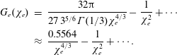 $$\begin{eqnarray}\displaystyle G_{e}(\unicode[STIX]{x1D712}_{e}) & = & \displaystyle \frac{32\unicode[STIX]{x03C0}}{27\,3^{5/6}\unicode[STIX]{x1D6E4}(1/3)\unicode[STIX]{x1D712}_{e}^{4/3}}-\frac{1}{\unicode[STIX]{x1D712}_{e}^{2}}+\cdots \nonumber\\ \displaystyle & {\approx} & \displaystyle \frac{0.5564}{\unicode[STIX]{x1D712}_{e}^{4/3}}-\frac{1}{\unicode[STIX]{x1D712}_{e}^{2}}+\cdots \,.\end{eqnarray}$$
However, expression (2.21) and the asymptotical dependences (2.22) and (2.23) are not convenient for implementation in computer codes. For the sake of calculation simplicity we shall use the following approximation
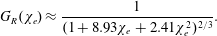 $$\begin{eqnarray}G_{R}(\unicode[STIX]{x1D712}_{e})\approx \frac{1}{(1+8.93\unicode[STIX]{x1D712}_{e}+2.41\unicode[STIX]{x1D712}_{e}^{2})^{2/3}}.\end{eqnarray}$$
Within the interval
 $0<\unicode[STIX]{x1D712}_{e}<10$
the accuracy of this approximation is better than 1 %.
$0<\unicode[STIX]{x1D712}_{e}<10$
the accuracy of this approximation is better than 1 %.
3 Electron motion in the standing EM wave formed by two counter-propagating EM pulses
3.1 EM field configuration
An electron interaction with an EM field formed by two counter-propagating waves has been addressed a number of times in high field theory using classical quantum electrodynamics approaches because it provides one of the basic EM configurations where important properties of a radiating electron can be revealed (e.g. see above cited publications Mendonca Reference Mendonca1983; Di Piazza et al. Reference Di Piazza, Muller, Hatsagortsyan and Keitel2012; Lehmann & Spatschek Reference Lehmann and Spatschek2012, Reference Lehmann and Spatschek2016; Gonoskov et al. Reference Gonoskov, Gonoskov, Harvey, Ilderton, Kim, Marklund, Mourou and Sergeev2013, Reference Gonoskov, Bashinov, Gonoskov, Harvey, Ilderton, Kim, Marklund, Mourou and Sergeev2014; Bashinov et al. Reference Bashinov, Kim and Sergeev2015; Bulanov et al. Reference Bulanov, Esirkepov, Kando, Koga, Kondo and Korn2015; Chang et al. Reference Chang, Qiao, Xu, Xu, Zhou, Yan, Wu, Borghesi, Zepf and He2015; Esirkepov et al. Reference Esirkepov, Bulanov, Koga, Kando, Kondo, Rosanov, Korn and Bulanov2015; Lobet et al. Reference Lobet, Ruyer, Debayle, D’Humiéres, Grech, Lemoine and Gremillet2015; Bashinov, Kumar & Kim Reference Bashinov, Kumar and Kim2016; Grismayer et al. Reference Grismayer, Vranic, Martins, Fonseca and Silva2016; Jirka et al. Reference Jirka, Klimo, Bulanov, Esirkepov, Gelfer, Bulanov, Weber and Korn2016; Kirk Reference Kirk2016). Here, we present the results of the analysis of electron motion in a standing EM wave in order to compare them below with the radiating electron behaviour in a more complicated EM configuration formed by three or four waves with various polarizations.
Here we consider an electron interaction with the electromagnetic field corresponding to two counter-propagating linearly polarized waves of equal amplitude,
 $(a_{0}/2)\cos (t+x)$
and
$(a_{0}/2)\cos (t+x)$
and
 $(a_{0}/2)\cos (t-x)$
, forming a standing wave. The field is given by the electromagnetic 4-potential
$(a_{0}/2)\cos (t-x)$
, forming a standing wave. The field is given by the electromagnetic 4-potential
 $$\begin{eqnarray}\boldsymbol{A}=a_{0}\cos t\cos x\boldsymbol{e}_{z}.\end{eqnarray}$$
This is a standing electromagnetic wave with zero magnetic and electric field nodes located at the coordinates
 $x=\pm \unicode[STIX]{x03C0}n$
and
$x=\pm \unicode[STIX]{x03C0}n$
and
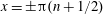 $x=\pm \unicode[STIX]{x03C0}(n+1/2)$
with
$x=\pm \unicode[STIX]{x03C0}(n+1/2)$
with
 $n=0,1,2,\ldots ,$
respectively.
$n=0,1,2,\ldots ,$
respectively.
Numerical integration of the electron motion equations with the radiation friction force in the form (2.20) shows different features of the electron dynamics depending on the electromagnetic wave amplitude and the dissipation parameter
 $\unicode[STIX]{x1D700}_{rad}$
.
$\unicode[STIX]{x1D700}_{rad}$
.
(a) Electron trajectories in the
 $(x,z)$
plane for initial conditions:
$(x,z)$
plane for initial conditions:
 $x(0)=0.01$
,
$x(0)=0.01$
,
 $z(0)=0$
,
$z(0)=0$
,
 $p_{x}(0)=0$
,
$p_{x}(0)=0$
,
 $p_{z}(0)=0$
. (b) Trajectory in the phase space
$p_{z}(0)=0$
. (b) Trajectory in the phase space
 $x,p_{x},p_{z}$
; (c) electron gamma-factor,
$x,p_{x},p_{z}$
; (c) electron gamma-factor,
 $\unicode[STIX]{x1D6FE}_{e}$
, versus the coordinate
$\unicode[STIX]{x1D6FE}_{e}$
, versus the coordinate
 $x$
; (d) parameter
$x$
; (d) parameter
 $\unicode[STIX]{x1D712}_{e}$
versus the coordinate
$\unicode[STIX]{x1D712}_{e}$
versus the coordinate
 $x$
, for the same initial conditions. The electromagnetic field amplitude is
$x$
, for the same initial conditions. The electromagnetic field amplitude is
 $a_{0}=617$
and the dissipation parameter is
$a_{0}=617$
and the dissipation parameter is
 $\unicode[STIX]{x1D700}_{rad}=1.2\times 10^{-8}$
. The coordinates, time and momentum are measured in
$\unicode[STIX]{x1D700}_{rad}=1.2\times 10^{-8}$
. The coordinates, time and momentum are measured in
 $2\unicode[STIX]{x03C0}c/\unicode[STIX]{x1D714}$
,
$2\unicode[STIX]{x03C0}c/\unicode[STIX]{x1D714}$
,
 $2\unicode[STIX]{x03C0}/\unicode[STIX]{x1D714}$
and
$2\unicode[STIX]{x03C0}/\unicode[STIX]{x1D714}$
and
 $m_{e}c$
units.
$m_{e}c$
units.

3.2 Relatively weak intensity limit
In the limit of relatively weak dissipation, which corresponds to domain I in figure 1, the electron trajectory wanders in the phase space and in the coordinate space as shown in figure 2. In this case the wave amplitude is
 $a_{0}=618$
. The dissipation parameter equals
$a_{0}=618$
. The dissipation parameter equals
 $\unicode[STIX]{x1D700}_{rad}=2\times 10^{-8}$
. The normalized critical QED field is
$\unicode[STIX]{x1D700}_{rad}=2\times 10^{-8}$
. The normalized critical QED field is
 $a_{S}=eE_{S}/m_{e}\unicode[STIX]{x1D714}c=m_{e}c^{2}/\hbar \unicode[STIX]{x1D714}=4\times 10^{5}$
. The parameter values correspond to the vicinity of the point
$a_{S}=eE_{S}/m_{e}\unicode[STIX]{x1D714}c=m_{e}c^{2}/\hbar \unicode[STIX]{x1D714}=4\times 10^{5}$
. The parameter values correspond to the vicinity of the point
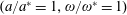 $(a/a^{\ast }=1,\unicode[STIX]{x1D714}/\unicode[STIX]{x1D714}^{\ast }=1)$
in figure 1(b). The integration time equals 75.
$(a/a^{\ast }=1,\unicode[STIX]{x1D714}/\unicode[STIX]{x1D714}^{\ast }=1)$
in figure 1(b). The integration time equals 75.
Figure 2 demonstrates a typical behaviour of the electron in the limit of relatively low EM wave amplitude. Figure 2(a,b) shows that the electron performs a random-walk-like motion for a long time, being intermittently trapped and untrapped in the vicinities of the zero electric field nodes, where the electric field vanishes. For this parameter choice the equilibrium trajectory at the electric field antinodes is unstable according to Bulanov et al. (Reference Bulanov, Esirkepov, Koga, Thomas and Bulanov2010a
) (see also Gong et al.
Reference Gong, Hu, Shou, Qiao, Chen, Xu, He and Yan2016). The maximum value of the electron gamma-factor,
 $\unicode[STIX]{x1D6FE}_{e}$
, whose dependence on the coordinate
$\unicode[STIX]{x1D6FE}_{e}$
, whose dependence on the coordinate
 $x$
is plotted in figure 2(c), reaches 700. In an oscillating electric field of amplitude
$x$
is plotted in figure 2(c), reaches 700. In an oscillating electric field of amplitude
 $a=618$
it would be equal to 618. The parameter
$a=618$
it would be equal to 618. The parameter
 $\unicode[STIX]{x1D712}_{e}$
(see figure 2
d) changes between zero and approximately 0.7, which corresponds, within an order of magnitude, to
$\unicode[STIX]{x1D712}_{e}$
(see figure 2
d) changes between zero and approximately 0.7, which corresponds, within an order of magnitude, to
 $(a_{0}/a_{S})\unicode[STIX]{x1D6FE}_{e}$
. The particle coordinates
$(a_{0}/a_{S})\unicode[STIX]{x1D6FE}_{e}$
. The particle coordinates
 $z$
versus time in figure 3, for initial coordinates
$z$
versus time in figure 3, for initial coordinates
 $x(0)=0.01$
–1, 0.2–2, 0.49–3 with other parameters the same as in figure 2, show its wandering along the coordinate
$x(0)=0.01$
–1, 0.2–2, 0.49–3 with other parameters the same as in figure 2, show its wandering along the coordinate
 $z$
. The particle over-leaping from one field period to another with small-scale oscillations in between seen in figure 3 may correspond to Lévy flights (see Lévy Reference Lévy1954; Metzler & Klafter Reference Metzler and Klafter2000; Zaslavsky Reference Zaslavsky2002; Metzler et al.
Reference Metzler, Chechkin, Gonchar and Klafter2007).
$z$
. The particle over-leaping from one field period to another with small-scale oscillations in between seen in figure 3 may correspond to Lévy flights (see Lévy Reference Lévy1954; Metzler & Klafter Reference Metzler and Klafter2000; Zaslavsky Reference Zaslavsky2002; Metzler et al.
Reference Metzler, Chechkin, Gonchar and Klafter2007).
Electron coordinate
 $z$
versus time for initial coordinates
$z$
versus time for initial coordinates
 $x(0)=0.01$
–1, 0.2–2, 0.49–3, other parameters are the same as in figure 2.
$x(0)=0.01$
–1, 0.2–2, 0.49–3, other parameters are the same as in figure 2.
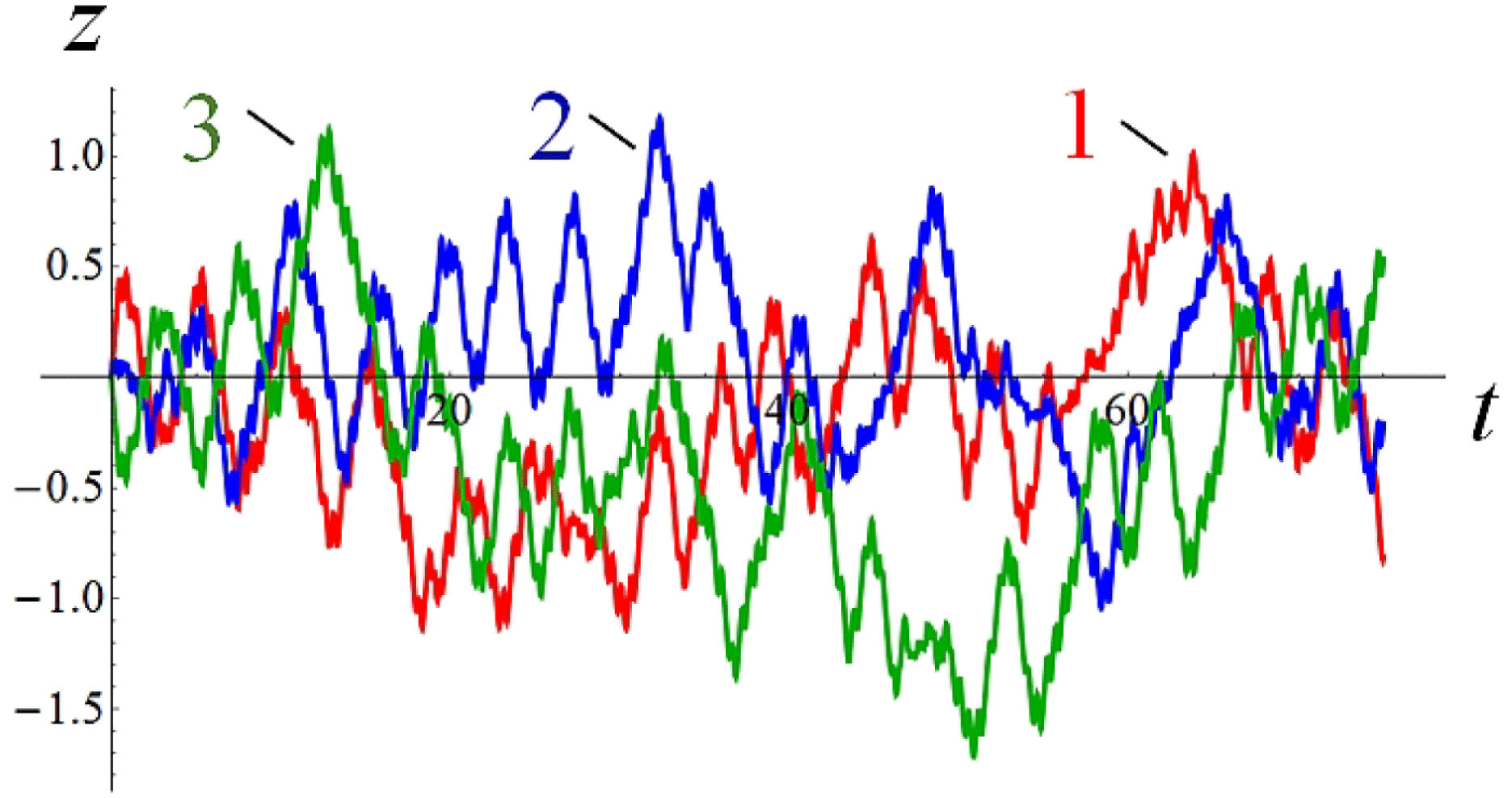
Figure 4 shows the Poincaré section for the motion of the particle with
 $x(0)=0.01$
positions in the phase plane
$x(0)=0.01$
positions in the phase plane
 $(p_{x},p_{z})$
at discrete times with the time step equal to the period of the driving force. The parameters are the same as in figure 2. The Poincaré section demonstrates that this process is stochastic.
$(p_{x},p_{z})$
at discrete times with the time step equal to the period of the driving force. The parameters are the same as in figure 2. The Poincaré section demonstrates that this process is stochastic.
The Poincaré sections showing the particle positions in the phase plane (
 $p_{x},p_{z}$
) at discrete times with the time step equal to the period of the driving force. The parameters are the same as in figure 2 for
$p_{x},p_{z}$
) at discrete times with the time step equal to the period of the driving force. The parameters are the same as in figure 2 for
 $x(0)=0.01$
.
$x(0)=0.01$
.
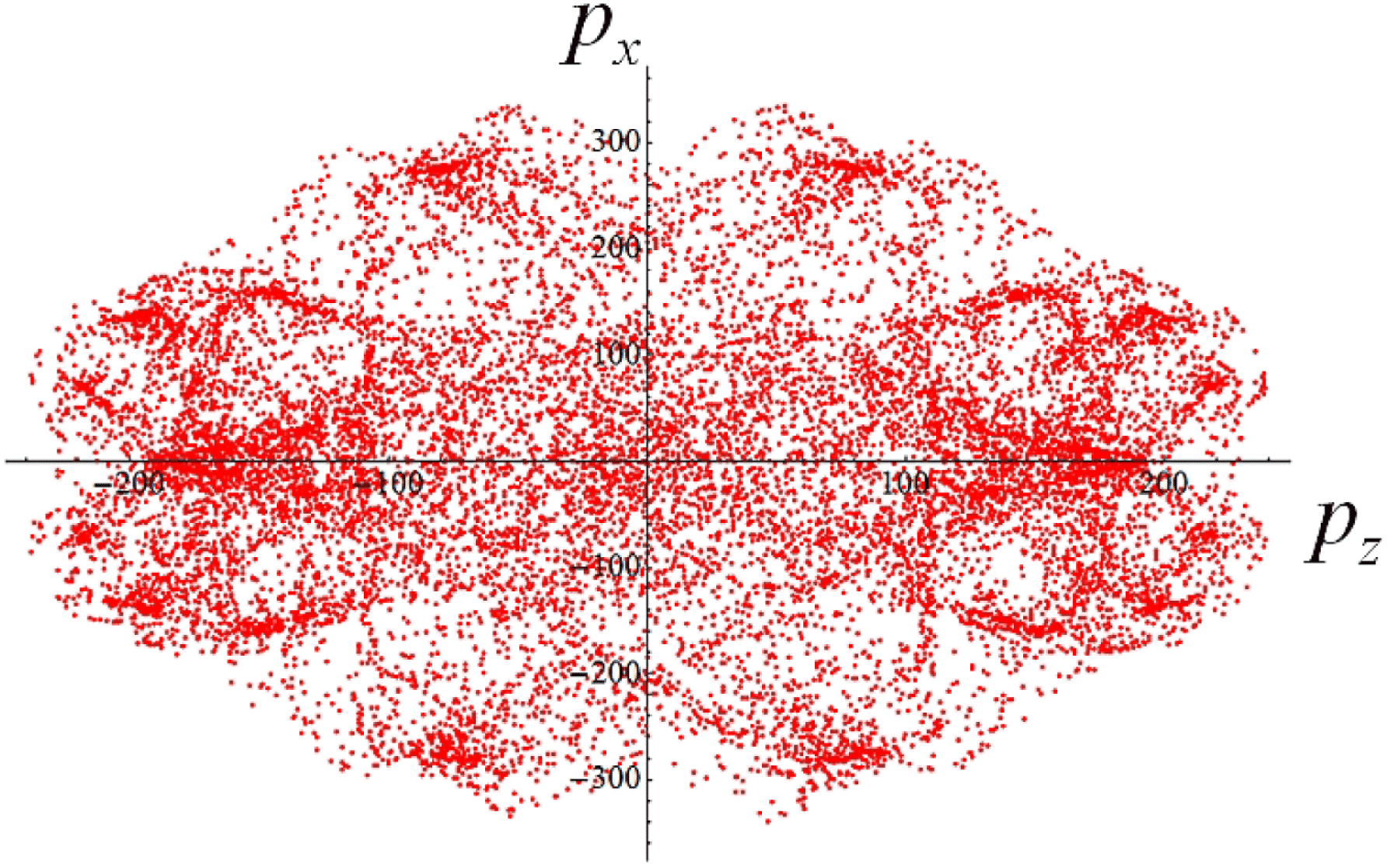
Dependences of
 $\text{Log}(\text{Var}[r]/t^{q})$
on
$\text{Log}(\text{Var}[r]/t^{q})$
on
 $\text{Log}(t)$
for
$\text{Log}(t)$
for
 $0<q<1.25$
for the parameters corresponding to figure 2.
$0<q<1.25$
for the parameters corresponding to figure 2.
3.3 Random walk
Now we analyse the time dependence of the random walk, assuming that the particle coordinates
 $x(t)$
and
$x(t)$
and
 $z(t)$
are random variables, i.e. the particle displacement in the
$z(t)$
are random variables, i.e. the particle displacement in the
 $(x,z)$
plane equal to
$(x,z)$
plane equal to
 $r=\sqrt{x^{2}+z^{2}}$
is also a random variable. As is known in statistics the behaviour of the random variable
$r=\sqrt{x^{2}+z^{2}}$
is also a random variable. As is known in statistics the behaviour of the random variable
 $f$
is characterized by the expectation
$f$
is characterized by the expectation
 $\unicode[STIX]{x1D707}=E[f]$
and variance
$\unicode[STIX]{x1D707}=E[f]$
and variance
 $\unicode[STIX]{x1D70E}^{2}=\text{Var}[f]$
defined as
$\unicode[STIX]{x1D70E}^{2}=\text{Var}[f]$
defined as
 $$\begin{eqnarray}E[f]=\lim _{t\rightarrow \infty }\frac{1}{t}\int ^{t}f(t)\,\text{d}t\end{eqnarray}$$
and
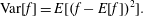 $$\begin{eqnarray}\text{Var}[f]=E[(f-E[f])^{2}].\end{eqnarray}$$
The definition of an expectation in the form (3.2) implies that the probability density function is taken to be a continuous uniform distribution equal to
 $1/t$
within the interval
$1/t$
within the interval
 $[0,t]$
. We assume here that the ergodicity of the processes is expected.
$[0,t]$
. We assume here that the ergodicity of the processes is expected.
If the random walk process is a Wiener process, which is also called ‘Brownian motion’, the variance of the walker’s coordinate
 $r(t)$
is proportional to time (e.g. see Durrett Reference Durrett1991). To examine whether or not the random walk seen in figures 2 and 3 is a Wiener process we plot in figure 5 the dependences of
$r(t)$
is proportional to time (e.g. see Durrett Reference Durrett1991). To examine whether or not the random walk seen in figures 2 and 3 is a Wiener process we plot in figure 5 the dependences of
 $\text{Log}(\text{Var}[r]/t^{q})$
on
$\text{Log}(\text{Var}[r]/t^{q})$
on
 $\text{Log}(t)$
for
$\text{Log}(t)$
for
 $0<q<1.75$
. For a Wiener process the parameter
$0<q<1.75$
. For a Wiener process the parameter
 $q$
should be equal to 1. As we can see, in our case of a random walk process the variance is proportional to
$q$
should be equal to 1. As we can see, in our case of a random walk process the variance is proportional to
 $t^{q}$
with
$t^{q}$
with
 $q\approx 1$
.
$q\approx 1$
.
Electron motion in the standing EM wave for
 $\unicode[STIX]{x1D700}_{rad}=6\times 10^{-9}$
,
$\unicode[STIX]{x1D700}_{rad}=6\times 10^{-9}$
,
 $a_{S}=8\times 10^{5}$
and
$a_{S}=8\times 10^{5}$
and
 $a_{0}=778$
for initial conditions:
$a_{0}=778$
for initial conditions:
 $x(0)=0.01$
,
$x(0)=0.01$
,
 $z(0)=0$
,
$z(0)=0$
,
 $p_{x}(0)=0$
,
$p_{x}(0)=0$
,
 $p_{z}(0)=0$
(red);
$p_{z}(0)=0$
(red);
 $x(0)=0.2$
,
$x(0)=0.2$
,
 $z(0)=0$
,
$z(0)=0$
,
 $p_{x}(0)=0$
,
$p_{x}(0)=0$
,
 $p_{z}(0)=0$
(blue);
$p_{z}(0)=0$
(blue);
 $x(0)=0.49$
,
$x(0)=0.49$
,
 $z(0)=0$
,
$z(0)=0$
,
 $p_{x}(0)=0$
,
$p_{x}(0)=0$
,
 $p_{z}(0)=0$
(green). (a) Trajectory in the
$p_{z}(0)=0$
(green). (a) Trajectory in the
 $x,z$
plane. Dashed line is the ponderomotive potential (3.4) versus the
$x,z$
plane. Dashed line is the ponderomotive potential (3.4) versus the
 $x$
coordinate; (b) electron trajectories in the
$x$
coordinate; (b) electron trajectories in the
 $(x,p_{x},p_{z})$
space. (c) Electron gamma-factor,
$(x,p_{x},p_{z})$
space. (c) Electron gamma-factor,
 $\unicode[STIX]{x1D6FE}_{e}$
, versus the coordinate
$\unicode[STIX]{x1D6FE}_{e}$
, versus the coordinate
 $x$
. (d) Parameter
$x$
. (d) Parameter
 $\unicode[STIX]{x1D712}_{e}$
versus the coordinate
$\unicode[STIX]{x1D712}_{e}$
versus the coordinate
 $x$
, for the same initial conditions.
$x$
, for the same initial conditions.
3.4 Moderate intensity regime
The situation qualitatively changes when the dissipation becomes more significant. In figure 1 this corresponds to the domain II. This case is illustrated in figure 6, for which the radiation friction parameter is
 $\unicode[STIX]{x1D700}_{rad}=6\times 10^{-9}$
, the normalized critical QED field is
$\unicode[STIX]{x1D700}_{rad}=6\times 10^{-9}$
, the normalized critical QED field is
 $a_{S}=8\times 10^{5}$
and the normalized laser field equals
$a_{S}=8\times 10^{5}$
and the normalized laser field equals
 $a_{0}=778$
. In figure 6 we present three trajectories for particles with initial conditions:
$a_{0}=778$
. In figure 6 we present three trajectories for particles with initial conditions:
 $x(0)=0.01$
,
$x(0)=0.01$
,
 $z(0)=0$
,
$z(0)=0$
,
 $p_{x}(0)=0$
,
$p_{x}(0)=0$
,
 $p_{z}(0)=0$
(red);
$p_{z}(0)=0$
(red);
 $x(0)=0.2$
,
$x(0)=0.2$
,
 $z(0)=0$
,
$z(0)=0$
,
 $p_{x}(0)=0$
,
$p_{x}(0)=0$
,
 $p_{z}(0)=0$
(blue);
$p_{z}(0)=0$
(blue);
 $x(0)=0.49$
,
$x(0)=0.49$
,
 $z(0)=0$
,
$z(0)=0$
,
 $p_{x}(0)=0$
,
$p_{x}(0)=0$
,
 $p_{z}(0)=0$
(green). As seen in figure 6(a), where the trajectories in the
$p_{z}(0)=0$
(green). As seen in figure 6(a), where the trajectories in the
 $x,z$
plane are shown, independent of the initial position all three trajectories end up in the vicinity of the plane
$x,z$
plane are shown, independent of the initial position all three trajectories end up in the vicinity of the plane
 $x=0.25$
. Here the EM wave electric field vanishes.
$x=0.25$
. Here the EM wave electric field vanishes.
At the coordinate
 $x=0.25$
the ponderomotive potential has a minimum. It is defined as
$x=0.25$
the ponderomotive potential has a minimum. It is defined as
 $$\begin{eqnarray}\unicode[STIX]{x1D6F1}(x)=\frac{1}{2\unicode[STIX]{x03C0}}\int _{-\unicode[STIX]{x03C0}}^{\unicode[STIX]{x03C0}}\left(\!\sqrt{1+A(x,t)^{2}}-1\right)\text{d}t\end{eqnarray}$$
with the vector potential
 $A(x,t)$
given by (3.1). The dashed curve in figure 6(a) presents the ponderomotive potential (3.4) dependence on the
$A(x,t)$
given by (3.1). The dashed curve in figure 6(a) presents the ponderomotive potential (3.4) dependence on the
 $x$
coordinate. In figure 6(b) electron trajectories in the
$x$
coordinate. In figure 6(b) electron trajectories in the
 $(x,p_{x},p_{z})$
space show the attractors, which have been analysed in detail in Esirkepov et al. (Reference Esirkepov, Bulanov, Koga, Kando, Kondo, Rosanov, Korn and Bulanov2015) (see figure 7, where the Poincaré section is presented for this case). Electron gamma-factor,
$(x,p_{x},p_{z})$
space show the attractors, which have been analysed in detail in Esirkepov et al. (Reference Esirkepov, Bulanov, Koga, Kando, Kondo, Rosanov, Korn and Bulanov2015) (see figure 7, where the Poincaré section is presented for this case). Electron gamma-factor,
 $\unicode[STIX]{x1D6FE}_{e}$
, versus the coordinate
$\unicode[STIX]{x1D6FE}_{e}$
, versus the coordinate
 $x$
presented in figure 6(c) correspond to the case when the dissipation limits the particle energy, which does not exceed the value determined by the amplitude of the EM wave being of the order of
$x$
presented in figure 6(c) correspond to the case when the dissipation limits the particle energy, which does not exceed the value determined by the amplitude of the EM wave being of the order of
 $a$
. Since the parameter
$a$
. Since the parameter
 $\unicode[STIX]{x1D712}_{e}(x)$
plotted in figure 6(d) is less than unity for all three trajectories, the equation of electron motion with the radiation friction force is still valid for this parameter range.
$\unicode[STIX]{x1D712}_{e}(x)$
plotted in figure 6(d) is less than unity for all three trajectories, the equation of electron motion with the radiation friction force is still valid for this parameter range.
In figure 7, we plot the Poincaré section for the particle with the same parameters as in figure 6 for
 $x(0)=0.01$
. Here, the particle positions are in the phase plane (
$x(0)=0.01$
. Here, the particle positions are in the phase plane (
 $x,p_{x}$
) at discrete times with the time step equal to the period of the driving force. The map pattern corresponds to the stochastic regime developed in the particle motion.
$x,p_{x}$
) at discrete times with the time step equal to the period of the driving force. The map pattern corresponds to the stochastic regime developed in the particle motion.
The Poincaré sections showing the particle positions in the phase plane (
 $x,p_{x}$
) at discrete times with the time step equal to the period of the driving force. The parameters are the same as in figure 6 for
$x,p_{x}$
) at discrete times with the time step equal to the period of the driving force. The parameters are the same as in figure 6 for
 $x(0)=0.01$
.
$x(0)=0.01$
.
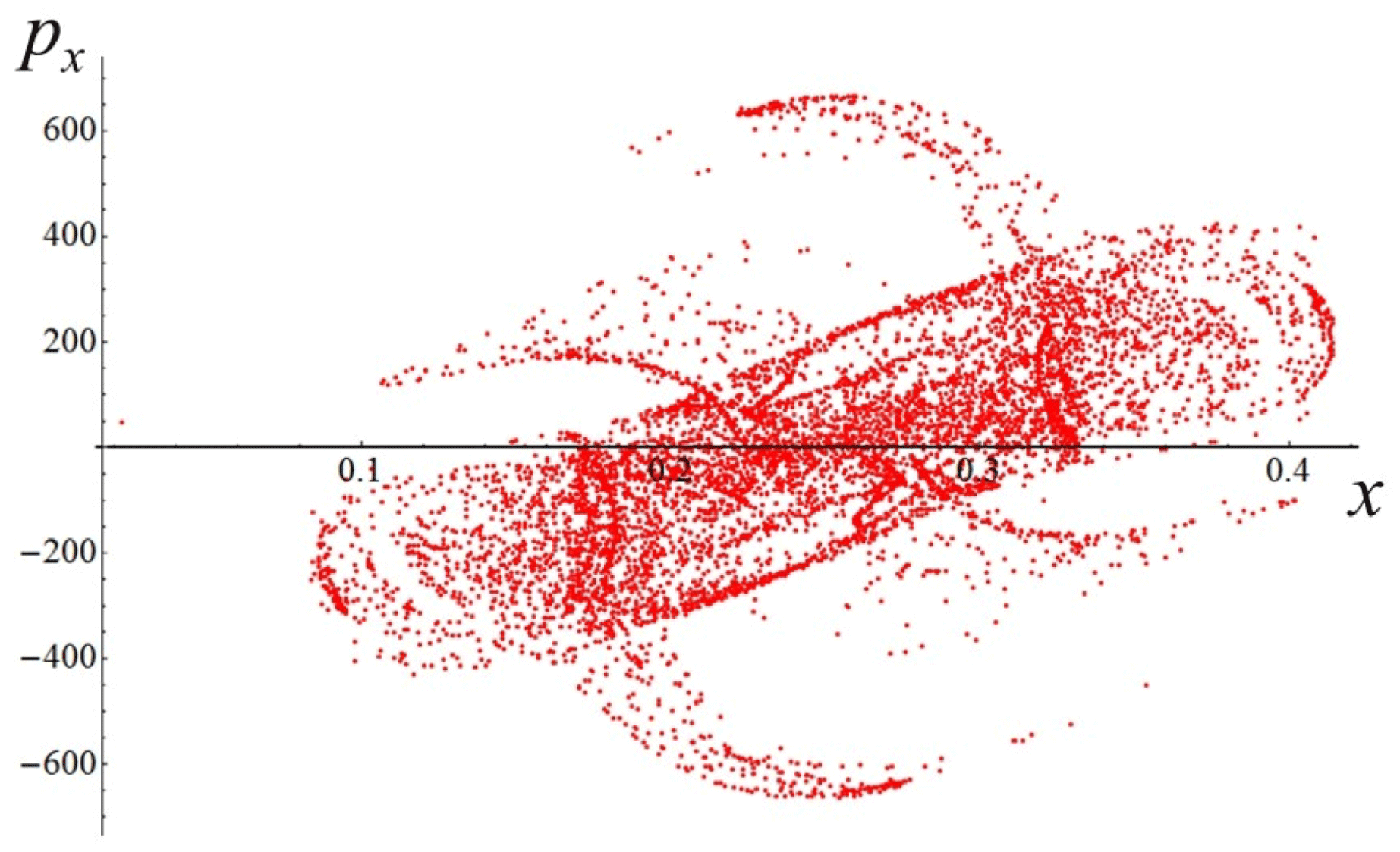
Electron motion in the standing EM wave for
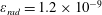 $\unicode[STIX]{x1D700}_{rad}=1.2\times 10^{-9}$
,
$\unicode[STIX]{x1D700}_{rad}=1.2\times 10^{-9}$
,
 $a_{S}=4\times 10^{6}$
,
$a_{S}=4\times 10^{6}$
,
 $a=1996$
for initial conditions:
$a=1996$
for initial conditions:
 $x(0)=0.01$
,
$x(0)=0.01$
,
 $z(0)=0$
,
$z(0)=0$
,
 $p_{x}(0)=0$
,
$p_{x}(0)=0$
,
 $p_{z}(0)=0$
(red);
$p_{z}(0)=0$
(red);
 $x(0)=0.2$
,
$x(0)=0.2$
,
 $z(0)=0$
,
$z(0)=0$
,
 $p_{x}(0)=0$
,
$p_{x}(0)=0$
,
 $p_{z}(0)=0$
(blue);
$p_{z}(0)=0$
(blue);
 $x(0)=0.49$
,
$x(0)=0.49$
,
 $z(0)=0$
,
$z(0)=0$
,
 $p_{x}(0)=0$
,
$p_{x}(0)=0$
,
 $p_{z}(0)=0$
(green). (a) Trajectory in the
$p_{z}(0)=0$
(green). (a) Trajectory in the
 $x,z$
plane. Inset shows zoomed trajectory for
$x,z$
plane. Inset shows zoomed trajectory for
 $x(0)=0.2$
. Dashed line is the ponderomotive potential (3.4) versus the
$x(0)=0.2$
. Dashed line is the ponderomotive potential (3.4) versus the
 $x$
coordinate; (b) electron trajectories in the
$x$
coordinate; (b) electron trajectories in the
 $(x,p_{x},p_{z})$
space. Inset shows zoomed trajectory for
$(x,p_{x},p_{z})$
space. Inset shows zoomed trajectory for
 $x(0)=0.2$
corresponding to a strange attractor (Esirkepov et al.
Reference Esirkepov, Bulanov, Koga, Kando, Kondo, Rosanov, Korn and Bulanov2015). (c) Electron gamma-factor,
$x(0)=0.2$
corresponding to a strange attractor (Esirkepov et al.
Reference Esirkepov, Bulanov, Koga, Kando, Kondo, Rosanov, Korn and Bulanov2015). (c) Electron gamma-factor,
 $\unicode[STIX]{x1D6FE}_{e}$
, versus the coordinate
$\unicode[STIX]{x1D6FE}_{e}$
, versus the coordinate
 $x$
. Inset shows zoomed
$x$
. Inset shows zoomed
 $\unicode[STIX]{x1D6FE}_{e}(x)$
for
$\unicode[STIX]{x1D6FE}_{e}(x)$
for
 $x(0)=0.2$
. (d) Parameter
$x(0)=0.2$
. (d) Parameter
 $\unicode[STIX]{x1D712}_{e}$
versus the coordinate
$\unicode[STIX]{x1D712}_{e}$
versus the coordinate
 $x$
, for the same initial conditions.
$x$
, for the same initial conditions.
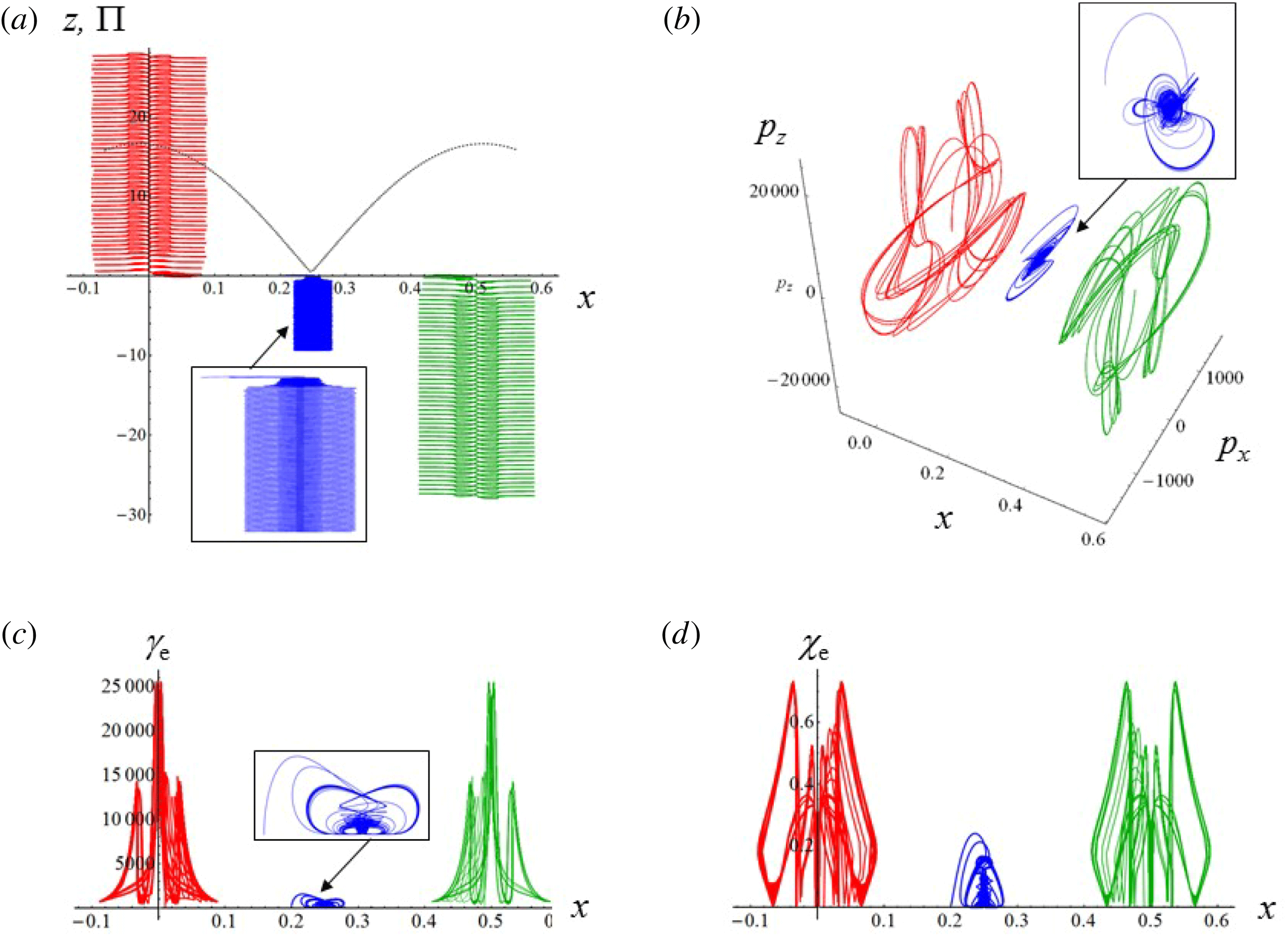
3.5 High intensity regime
If we choose the parameters in a such the way that the dissipation becomes even more significant, when we approach domain IV in figure 1, the particle behaviour becomes counterintuitive, as can be seen in figure 8, for which the radiation friction parameter is
 $\unicode[STIX]{x1D700}_{rad}=1.2\times 10^{-9}$
, the normalized critical QED field is
$\unicode[STIX]{x1D700}_{rad}=1.2\times 10^{-9}$
, the normalized critical QED field is
 $a_{S}=4\times 10^{6}$
and the normalized laser field equals
$a_{S}=4\times 10^{6}$
and the normalized laser field equals
 $a_{0}=1996$
. There we present three electron trajectories for the same initial conditions as in figure 4:
$a_{0}=1996$
. There we present three electron trajectories for the same initial conditions as in figure 4:
 $x(0)=0.01$
,
$x(0)=0.01$
,
 $z(0)=0$
,
$z(0)=0$
,
 $p_{x}(0)=0$
,
$p_{x}(0)=0$
,
 $p_{z}(0)=0$
(red);
$p_{z}(0)=0$
(red);
 $x(0)=0.2$
,
$x(0)=0.2$
,
 $z(0)=0$
,
$z(0)=0$
,
 $p_{x}(0)=0$
,
$p_{x}(0)=0$
,
 $p_{z}(0)=0$
(blue);
$p_{z}(0)=0$
(blue);
 $x(0)=0.49$
,
$x(0)=0.49$
,
 $z(0)=0$
,
$z(0)=0$
,
 $p_{x}(0)=0$
,
$p_{x}(0)=0$
,
 $p_{z}(0)=0$
(green). Trajectories in the
$p_{z}(0)=0$
(green). Trajectories in the
 $x,z$
plane (figure 6
a) are principally different depending on where the particle has been initially located. For
$x,z$
plane (figure 6
a) are principally different depending on where the particle has been initially located. For
 $x(0)=0.2$
the trajectory remains in the vicinity of the ponderomotive potential minimum similarly to the case discussed above (figure 6). The dashed line is the ponderomotive potential (3.4) versus the
$x(0)=0.2$
the trajectory remains in the vicinity of the ponderomotive potential minimum similarly to the case discussed above (figure 6). The dashed line is the ponderomotive potential (3.4) versus the
 $x$
coordinate. In contrast, particles with initial coordinates near the maximum of the ponderomotive potential are trapped there (similar behaviour was noted in Gonoskov et al. (Reference Gonoskov, Bashinov, Gonoskov, Harvey, Ilderton, Kim, Marklund, Mourou and Sergeev2014)).
$x$
coordinate. In contrast, particles with initial coordinates near the maximum of the ponderomotive potential are trapped there (similar behaviour was noted in Gonoskov et al. (Reference Gonoskov, Bashinov, Gonoskov, Harvey, Ilderton, Kim, Marklund, Mourou and Sergeev2014)).
In figure 8(b) the electron trajectories in the
 $(x,p_{x},p_{z})$
space show behaviour typical for limit circles and attractors. The inset shows the zoomed trajectory for
$(x,p_{x},p_{z})$
space show behaviour typical for limit circles and attractors. The inset shows the zoomed trajectory for
 $x(0)=0.2$
corresponding to a strange attractor (Esirkepov et al.
Reference Esirkepov, Bulanov, Koga, Kando, Kondo, Rosanov, Korn and Bulanov2015). The trajectories with
$x(0)=0.2$
corresponding to a strange attractor (Esirkepov et al.
Reference Esirkepov, Bulanov, Koga, Kando, Kondo, Rosanov, Korn and Bulanov2015). The trajectories with
 $x(0)=0.01$
and
$x(0)=0.01$
and
 $x(0)=0.49$
demonstrate regular limit circles. It follows from figure 8(c) that the electron gamma-factor,
$x(0)=0.49$
demonstrate regular limit circles. It follows from figure 8(c) that the electron gamma-factor,
 $\unicode[STIX]{x1D6FE}_{e}$
, has a moderate value for the electron trapped near the ponderomotive potential minimum (the inset shows zoomed
$\unicode[STIX]{x1D6FE}_{e}$
, has a moderate value for the electron trapped near the ponderomotive potential minimum (the inset shows zoomed
 $\unicode[STIX]{x1D6FE}_{e}(x)$
for
$\unicode[STIX]{x1D6FE}_{e}(x)$
for
 $x(0)=0.2$
), and the particles are efficiently accelerated when they are trapped in the region at the ponderomotive potential maximum. For the parameters chosen,
$x(0)=0.2$
), and the particles are efficiently accelerated when they are trapped in the region at the ponderomotive potential maximum. For the parameters chosen,
 $\unicode[STIX]{x1D712}_{e}(x)$
plotted in figure 8(d) remains less than unity for all three trajectories, i.e. the QED effects are finite but relatively weak.
$\unicode[STIX]{x1D712}_{e}(x)$
plotted in figure 8(d) remains less than unity for all three trajectories, i.e. the QED effects are finite but relatively weak.
In figure 9, we plot the Poincaré section showing the particle with
 $x(0)=0.49$
position in the phase plane (
$x(0)=0.49$
position in the phase plane (
 $x,p_{x}$
) at discrete times with the time step equal to the period of the driving force. The parameters are the same as in figure 8 for
$x,p_{x}$
) at discrete times with the time step equal to the period of the driving force. The parameters are the same as in figure 8 for
 $x(0)=0.49$
. Although the map pattern is complicated it does not contain curve broadening, i.e. does not indicate a stochastic regime of the particle motion.
$x(0)=0.49$
. Although the map pattern is complicated it does not contain curve broadening, i.e. does not indicate a stochastic regime of the particle motion.
The Poincaré sections showing the particle positions in the phase plane (
 $x,p_{x}$
) at discrete times with the time step equal to the period of the driving force. The parameters are the same as in figure 8 for
$x,p_{x}$
) at discrete times with the time step equal to the period of the driving force. The parameters are the same as in figure 8 for
 $x(0)=0.49$
.
$x(0)=0.49$
.
In the next section we discuss the mechanism of dissipative particle trapping in the vicinity of the ponderomotive potential maximum which can explain the observed effects (see also Fedotov et al. Reference Fedotov, Elkina, Gelfer, Narozhny and Ruhl2014 and Esirkepov & Bulanov Reference Esirkepov and Bulanov2017).
4 Simple model of the stabilization of the particle motion in an oscillating field due to the nonlinear friction
Let us consider a particle motion in a fast oscillating field in a way similar to Landau & Lifshitz (Reference Landau and Lifshitz1976). As in Landau & Lifshitz (Reference Landau and Lifshitz1976) for the sake of simplicity of calculations we assume non-relativistic electron motion in one dimension, where the force acting on the particle depends on the coordinate
 $x$
and time
$x$
and time
 $t$
. In contrast to the consideration in Landau & Lifshitz (Reference Landau and Lifshitz1976), we take into account the effects of the friction. The equation of particle motion is
$t$
. In contrast to the consideration in Landau & Lifshitz (Reference Landau and Lifshitz1976), we take into account the effects of the friction. The equation of particle motion is
 $$\begin{eqnarray}\ddot{x}+\unicode[STIX]{x1D705}(F){\dot{x}}=F.\end{eqnarray}$$
Here a dot stands for the time derivative and
 $\unicode[STIX]{x1D705}(F)$
is the friction coefficient. It is assumed to depend on the rapidly oscillating driving force,
$\unicode[STIX]{x1D705}(F)$
is the friction coefficient. It is assumed to depend on the rapidly oscillating driving force,
 $$\begin{eqnarray}F(x,t)=f_{1}(x)\cos \unicode[STIX]{x1D714}t+f_{2}(x)\sin \unicode[STIX]{x1D714}t.\end{eqnarray}$$
We seek a solution of (4.1), assuming that it can be written as a sum of two parts,
 $$\begin{eqnarray}x(t)=X(t)+\unicode[STIX]{x1D709}(t),\end{eqnarray}$$
where
 $X(t)$
slowly varies with time and
$X(t)$
slowly varies with time and
 $\unicode[STIX]{x1D709}(t)$
is a small fast oscillating periodic function,
$\unicode[STIX]{x1D709}(t)$
is a small fast oscillating periodic function,
 $|\unicode[STIX]{x1D709}|\ll |X|$
.
$|\unicode[STIX]{x1D709}|\ll |X|$
.
We also assume that the time average of the function
 $\unicode[STIX]{x1D709}(t)$
over the oscillation period
$\unicode[STIX]{x1D709}(t)$
over the oscillation period
 $2\unicode[STIX]{x03C0}/\unicode[STIX]{x1D714}$
is zero. Introducing the notation
$2\unicode[STIX]{x03C0}/\unicode[STIX]{x1D714}$
is zero. Introducing the notation
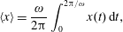 $$\begin{eqnarray}\langle x\rangle =\frac{\unicode[STIX]{x1D714}}{2\unicode[STIX]{x03C0}}\int _{0}^{2\unicode[STIX]{x03C0}/\unicode[STIX]{x1D714}}x(t)\,\text{d}t,\end{eqnarray}$$
we obtain
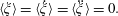 $$\begin{eqnarray}\langle \unicode[STIX]{x1D709}\rangle =\langle \dot{\unicode[STIX]{x1D709}}\rangle =\langle \ddot{\unicode[STIX]{x1D709}}\rangle =0.\end{eqnarray}$$
Therefore, we have
 $\langle x\rangle =X(t)$
, i.e. the function
$\langle x\rangle =X(t)$
, i.e. the function
 $X(t)$
describes the slow particle motion averaged over the fast oscillations,
$X(t)$
describes the slow particle motion averaged over the fast oscillations,
 $\langle X\rangle \approx X(t)$
.
$\langle X\rangle \approx X(t)$
.
Substituting (4.3) into the equation of particle motion (4.1) and expanding the functions
 $\unicode[STIX]{x1D705}(x,t)$
and
$\unicode[STIX]{x1D705}(x,t)$
and
 $F(x,t)$
in powers of
$F(x,t)$
in powers of
 $\unicode[STIX]{x1D709}$
, i.e. writing
$\unicode[STIX]{x1D709}$
, i.e. writing
 $\unicode[STIX]{x1D705}(x,t)\approx \unicode[STIX]{x1D705}(X,t)+\unicode[STIX]{x1D709}\unicode[STIX]{x2202}_{X}\unicode[STIX]{x1D705}(X,t)$
and
$\unicode[STIX]{x1D705}(x,t)\approx \unicode[STIX]{x1D705}(X,t)+\unicode[STIX]{x1D709}\unicode[STIX]{x2202}_{X}\unicode[STIX]{x1D705}(X,t)$
and
 $F(x,t)\approx F(X,t)+\unicode[STIX]{x1D709}\unicode[STIX]{x2202}_{X}F(X,t)$
, we obtain
$F(x,t)\approx F(X,t)+\unicode[STIX]{x1D709}\unicode[STIX]{x2202}_{X}F(X,t)$
, we obtain
 $$\begin{eqnarray}\ddot{X}+\ddot{\unicode[STIX]{x1D709}}+\unicode[STIX]{x1D705}{\dot{X}}+\unicode[STIX]{x1D705}\dot{\unicode[STIX]{x1D709}}+\unicode[STIX]{x1D709}{\dot{X}}\unicode[STIX]{x2202}_{X}\unicode[STIX]{x1D705}+\unicode[STIX]{x1D709}\dot{\unicode[STIX]{x1D709}}\unicode[STIX]{x2202}_{X}\unicode[STIX]{x1D705}=F+\unicode[STIX]{x1D709}\unicode[STIX]{x2202}_{X}F,\end{eqnarray}$$
where
 $\unicode[STIX]{x2202}_{X}$
is the partial derivative with respect to the first argument of functions
$\unicode[STIX]{x2202}_{X}$
is the partial derivative with respect to the first argument of functions
 $\unicode[STIX]{x1D705}(X,t)$
and
$\unicode[STIX]{x1D705}(X,t)$
and
 $F(X,t)$
. This equation contains slowly varying and fast oscillating terms, which apparently should be separately equal to each other. In the zeroth-order approximation with respect to small function
$F(X,t)$
. This equation contains slowly varying and fast oscillating terms, which apparently should be separately equal to each other. In the zeroth-order approximation with respect to small function
 $\unicode[STIX]{x1D709}$
and the time derivatives of the slow function
$\unicode[STIX]{x1D709}$
and the time derivatives of the slow function
 $X$
, we find the equation for the fast oscillating term
$X$
, we find the equation for the fast oscillating term
 $$\begin{eqnarray}\ddot{\unicode[STIX]{x1D709}}+\unicode[STIX]{x1D705}\dot{\unicode[STIX]{x1D709}}=F.\end{eqnarray}$$
Here we neglect the terms proportional to
 $\unicode[STIX]{x1D709}$
. The time derivatives
$\unicode[STIX]{x1D709}$
. The time derivatives
 $\ddot{\unicode[STIX]{x1D709}}$
and
$\ddot{\unicode[STIX]{x1D709}}$
and
 $\dot{\unicode[STIX]{x1D709}}$
are not small, being proportional to
$\dot{\unicode[STIX]{x1D709}}$
are not small, being proportional to
 $\unicode[STIX]{x1D714}^{2}$
and
$\unicode[STIX]{x1D714}^{2}$
and
 $\unicode[STIX]{x1D714}$
, respectively. They are assumed to be much greater than
$\unicode[STIX]{x1D714}$
, respectively. They are assumed to be much greater than
 $\ddot{X}$
and
$\ddot{X}$
and
 ${\dot{X}}$
. The friction coefficient
${\dot{X}}$
. The friction coefficient
 $\unicode[STIX]{x1D705}$
is not necessarily small.
$\unicode[STIX]{x1D705}$
is not necessarily small.
Integration of (4.7), assuming
 $X$
to be constant, yields
$X$
to be constant, yields
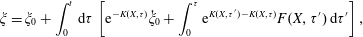 $$\begin{eqnarray}\displaystyle & \displaystyle \unicode[STIX]{x1D709}=\unicode[STIX]{x1D709}_{0}+\int _{0}^{t}\,\text{d}\unicode[STIX]{x1D70F}\left[\text{e}^{-K(X,\unicode[STIX]{x1D70F})}\dot{\unicode[STIX]{x1D709}}_{0}+\int _{0}^{\unicode[STIX]{x1D70F}}\text{e}^{K(X,\unicode[STIX]{x1D70F}^{\prime })-K(X,\unicode[STIX]{x1D70F})}F(X,\unicode[STIX]{x1D70F}^{\prime })\,\text{d}\unicode[STIX]{x1D70F}^{\prime }\right], & \displaystyle\end{eqnarray}$$
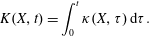 $$\begin{eqnarray}\displaystyle & \displaystyle K(X,t)=\int _{0}^{t}\unicode[STIX]{x1D705}(X,\unicode[STIX]{x1D70F})\,\text{d}\unicode[STIX]{x1D70F}. & \displaystyle\end{eqnarray}$$
Assuming that
 $K(X,t)$
can be approximated by
$K(X,t)$
can be approximated by
 $K(X,t)\approx \langle \unicode[STIX]{x1D705}\rangle t$
, where
$K(X,t)\approx \langle \unicode[STIX]{x1D705}\rangle t$
, where
 $\langle \unicode[STIX]{x1D705}\rangle$
is the time-averaged friction coefficient, in the limit
$\langle \unicode[STIX]{x1D705}\rangle$
is the time-averaged friction coefficient, in the limit
 $t\gg 1/\langle \unicode[STIX]{x1D705}\rangle$
we obtain
$t\gg 1/\langle \unicode[STIX]{x1D705}\rangle$
we obtain
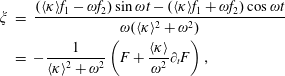 $$\begin{eqnarray}\displaystyle \unicode[STIX]{x1D709} & = & \displaystyle \frac{(\langle \unicode[STIX]{x1D705}\rangle f_{1}-\unicode[STIX]{x1D714}f_{2})\sin \unicode[STIX]{x1D714}t-(\langle \unicode[STIX]{x1D705}\rangle f_{1}+\unicode[STIX]{x1D714}f_{2})\cos \unicode[STIX]{x1D714}t}{\unicode[STIX]{x1D714}(\langle \unicode[STIX]{x1D705}\rangle ^{2}+\unicode[STIX]{x1D714}^{2})}\nonumber\\ \displaystyle & = & \displaystyle -\frac{1}{\langle \unicode[STIX]{x1D705}\rangle ^{2}+\unicode[STIX]{x1D714}^{2}}\left(F+\frac{\langle \unicode[STIX]{x1D705}\rangle }{\unicode[STIX]{x1D714}^{2}}\unicode[STIX]{x2202}_{t}F\right),\end{eqnarray}$$
with
 $\unicode[STIX]{x2202}_{t}F=\unicode[STIX]{x2202}F(X,t)/\unicode[STIX]{x2202}t|_{X=\text{const}}$
. Here we assume the initial condition
$\unicode[STIX]{x2202}_{t}F=\unicode[STIX]{x2202}F(X,t)/\unicode[STIX]{x2202}t|_{X=\text{const}}$
. Here we assume the initial condition
 $\unicode[STIX]{x1D709}_{0}=-(f_{2}+\unicode[STIX]{x1D714}\dot{\unicode[STIX]{x1D709}}_{0})/(\langle \unicode[STIX]{x1D705}\rangle \unicode[STIX]{x1D714})$
.
$\unicode[STIX]{x1D709}_{0}=-(f_{2}+\unicode[STIX]{x1D714}\dot{\unicode[STIX]{x1D709}}_{0})/(\langle \unicode[STIX]{x1D705}\rangle \unicode[STIX]{x1D714})$
.
Averaging (4.6) over time and taking into account that
 $\langle F(X,t)\rangle \approx 0$
for nearly constant
$\langle F(X,t)\rangle \approx 0$
for nearly constant
 $X(t)$
, we obtain
$X(t)$
, we obtain
 $$\begin{eqnarray}\ddot{X}+(\langle \unicode[STIX]{x1D705}\rangle +\langle \unicode[STIX]{x1D709}\unicode[STIX]{x2202}_{X}\unicode[STIX]{x1D705}\rangle ){\dot{X}}=\langle \unicode[STIX]{x1D709}\unicode[STIX]{x2202}_{X}F\rangle -\langle \unicode[STIX]{x1D709}\dot{\unicode[STIX]{x1D709}}\unicode[STIX]{x2202}_{X}\unicode[STIX]{x1D705}\rangle .\end{eqnarray}$$
Substituting expression (4.10) into the right-hand side of (4.11), for the first term we obtain
 $$\begin{eqnarray}\langle \unicode[STIX]{x1D709}\unicode[STIX]{x2202}_{X}F\rangle =-\frac{\unicode[STIX]{x2202}_{X}(f_{1}^{2}+f_{2}^{2})}{4(\langle \unicode[STIX]{x1D705}\rangle ^{2}+\unicode[STIX]{x1D714}^{2})}-\frac{\langle \unicode[STIX]{x1D705}\rangle (f_{2}\unicode[STIX]{x2202}_{X}f_{1}-f_{1}\unicode[STIX]{x2202}_{X}f_{2})}{2\unicode[STIX]{x1D714}(\langle \unicode[STIX]{x1D705}\rangle ^{2}+\unicode[STIX]{x1D714}^{2})}.\end{eqnarray}$$
The first term on the right-hand side of (4.12) is the well-known ponderomotive force (Landau & Lifshitz Reference Landau and Lifshitz1976) where the friction effect is taken into account. The last term on the right-hand side, proportional to the friction coefficient, can change signs for
 $f_{2}\unicode[STIX]{x2202}_{X}f_{1}\neq f_{1}\unicode[STIX]{x2202}_{X}f_{2}$
depending on whether
$f_{2}\unicode[STIX]{x2202}_{X}f_{1}\neq f_{1}\unicode[STIX]{x2202}_{X}f_{2}$
depending on whether
 $f_{2}\unicode[STIX]{x2202}_{X}f_{1}>f_{1}\unicode[STIX]{x2202}_{X}f_{2}$
or
$f_{2}\unicode[STIX]{x2202}_{X}f_{1}>f_{1}\unicode[STIX]{x2202}_{X}f_{2}$
or
 $f_{2}\unicode[STIX]{x2202}_{X}f_{1}<f_{1}\unicode[STIX]{x2202}_{X}f_{2}$
. It vanishes if
$f_{2}\unicode[STIX]{x2202}_{X}f_{1}<f_{1}\unicode[STIX]{x2202}_{X}f_{2}$
. It vanishes if
 $f_{2}\unicode[STIX]{x2202}_{X}f_{1}=f_{1}\unicode[STIX]{x2202}_{X}f_{2}$
,
$f_{2}\unicode[STIX]{x2202}_{X}f_{1}=f_{1}\unicode[STIX]{x2202}_{X}f_{2}$
,
 $f_{1}\neq 0$
,
$f_{1}\neq 0$
,
 $f_{2}=0$
or
$f_{2}=0$
or
 $f_{2}\neq 0$
,
$f_{2}\neq 0$
,
 $f_{1}=0$
.
$f_{1}=0$
.
The actual form of the last term on the right-hand side of (4.11) is determined by the specific dependence of the friction coefficient
 $\unicode[STIX]{x1D705}$
on the driver force. As an example, we consider the case when this dependence is quadratic, i.e.
$\unicode[STIX]{x1D705}$
on the driver force. As an example, we consider the case when this dependence is quadratic, i.e.
 $\unicode[STIX]{x1D705}=\unicode[STIX]{x1D708}F^{2}$
, with a constant
$\unicode[STIX]{x1D705}=\unicode[STIX]{x1D708}F^{2}$
, with a constant
 $\unicode[STIX]{x1D708}$
. Then we obtain
$\unicode[STIX]{x1D708}$
. Then we obtain
 $$\begin{eqnarray}-\langle \unicode[STIX]{x1D709}\dot{\unicode[STIX]{x1D709}}\unicode[STIX]{x2202}_{X}\unicode[STIX]{x1D705}\rangle =\frac{\unicode[STIX]{x1D708}\langle \unicode[STIX]{x1D705}\rangle \unicode[STIX]{x2202}_{X}(f_{1}^{2}+f_{2}^{2})^{2}}{8(\langle \unicode[STIX]{x1D705}\rangle ^{2}+\unicode[STIX]{x1D714}^{2})^{2}}+\frac{\unicode[STIX]{x1D708}(\langle \unicode[STIX]{x1D705}\rangle ^{2}-\unicode[STIX]{x1D714}^{2})(f_{1}^{2}+f_{2}^{2})(f_{2}\unicode[STIX]{x2202}_{X}f_{1}-f_{1}\unicode[STIX]{x2202}_{X}f_{2})}{4\unicode[STIX]{x1D714}(\langle \unicode[STIX]{x1D705}\rangle ^{2}+\unicode[STIX]{x1D714}^{2})^{2}}\end{eqnarray}$$
and the time-averaged friction coefficient becomes
 $\langle \unicode[STIX]{x1D705}\rangle =\unicode[STIX]{x1D708}(f_{1}^{2}+f_{2}^{2})/2$
. In addition,
$\langle \unicode[STIX]{x1D705}\rangle =\unicode[STIX]{x1D708}(f_{1}^{2}+f_{2}^{2})/2$
. In addition,
 $\langle \unicode[STIX]{x1D709}\unicode[STIX]{x2202}_{X}\unicode[STIX]{x1D705}\rangle =0$
.
$\langle \unicode[STIX]{x1D709}\unicode[STIX]{x2202}_{X}\unicode[STIX]{x1D705}\rangle =0$
.
For the sake of simplicity we further assume that
 $f_{2}=0$
in expression (4.2) for the driver force. Then, (4.12) and (4.13) are simplified and we finally obtain the equation for the slowly varying function
$f_{2}=0$
in expression (4.2) for the driver force. Then, (4.12) and (4.13) are simplified and we finally obtain the equation for the slowly varying function
 $X(t)$
:
$X(t)$
:
 $$\begin{eqnarray}\ddot{X}+\frac{\unicode[STIX]{x1D708}f_{1}^{2}}{2}{\dot{X}}=-\frac{\unicode[STIX]{x2202}_{X}f_{1}^{2}}{\unicode[STIX]{x1D708}^{2}f_{1}^{4}+4\unicode[STIX]{x1D714}^{2}}+\frac{2\unicode[STIX]{x1D708}^{2}\unicode[STIX]{x2202}_{X}f_{1}^{6}}{3(\unicode[STIX]{x1D708}^{2}f_{1}^{4}+4\unicode[STIX]{x1D714}^{2})^{2}}.\end{eqnarray}$$
The first term on the right-hand side corresponds to the ponderomotive force, the last term is the drag force induced by the friction.
As we can see, the ponderomotive force (4.12) and the drag force due to the friction (4.13) have different signs in (4.14). If
 $|\unicode[STIX]{x1D708}|>2\unicode[STIX]{x1D714}/f_{1}^{2}$
, the drag force exceeds in magnitude the ponderomotive force.
$|\unicode[STIX]{x1D708}|>2\unicode[STIX]{x1D714}/f_{1}^{2}$
, the drag force exceeds in magnitude the ponderomotive force.
Numerical integration of the equation of motion (4.1) with
 $$\begin{eqnarray}F(x,t)=f_{0}\exp (-(x/l_{0})^{2})\cos \unicode[STIX]{x1D714}t\quad \text{and}\quad \unicode[STIX]{x1D705}=\unicode[STIX]{x1D708}F^{2}\end{eqnarray}$$
reveals the main features of the behaviour predicted within the framework of the simple model approximation. The solutions for the cases of relatively weak and relatively strong driver force are plotted in figure 10. The parameters are as follows. The driver frequency and the friction coefficient values are
 $\unicode[STIX]{x1D714}=1$
and
$\unicode[STIX]{x1D714}=1$
and
 $\unicode[STIX]{x1D708}=0.1$
, respectively. The driver width equals
$\unicode[STIX]{x1D708}=0.1$
, respectively. The driver width equals
 $l_{0}=5$
. The initial coordinate and velocity are
$l_{0}=5$
. The initial coordinate and velocity are
 $x_{0}=3$
and
$x_{0}=3$
and
 ${\dot{x}}_{0}=1$
in both cases. The driver amplitude is equal to
${\dot{x}}_{0}=1$
in both cases. The driver amplitude is equal to
 $f_{0}=5\sqrt{2\unicode[STIX]{x1D714}/\unicode[STIX]{x1D708}}$
in the case of the weak driver and is equal to
$f_{0}=5\sqrt{2\unicode[STIX]{x1D714}/\unicode[STIX]{x1D708}}$
in the case of the weak driver and is equal to
 $f_{0}=15\sqrt{2\unicode[STIX]{x1D714}/\unicode[STIX]{x1D708}}$
in the case of the strong driver. As we see in figure 10(a,b), in the case of weak nonlinearity, the particle being pushed outwards by the ponderomotive force having performed several oscillations leaves the region where the driver force is localized. In contrast, in the limit of strong nonlinearity, the friction drag force prevents the particle from leaving the driver localization region resulting in its slow drift inwards (figure 10
c,d).
$f_{0}=15\sqrt{2\unicode[STIX]{x1D714}/\unicode[STIX]{x1D708}}$
in the case of the strong driver. As we see in figure 10(a,b), in the case of weak nonlinearity, the particle being pushed outwards by the ponderomotive force having performed several oscillations leaves the region where the driver force is localized. In contrast, in the limit of strong nonlinearity, the friction drag force prevents the particle from leaving the driver localization region resulting in its slow drift inwards (figure 10
c,d).
The solutions of (4.1) in the case of relatively weak driver force (a,b), and for the case of relatively strong driver force (c,d). (a,c) Dependence of the particle coordinate on time. (b,d) The particle trajectory in the phase plane
 $(x,{\dot{x}})$
.
$(x,{\dot{x}})$
.
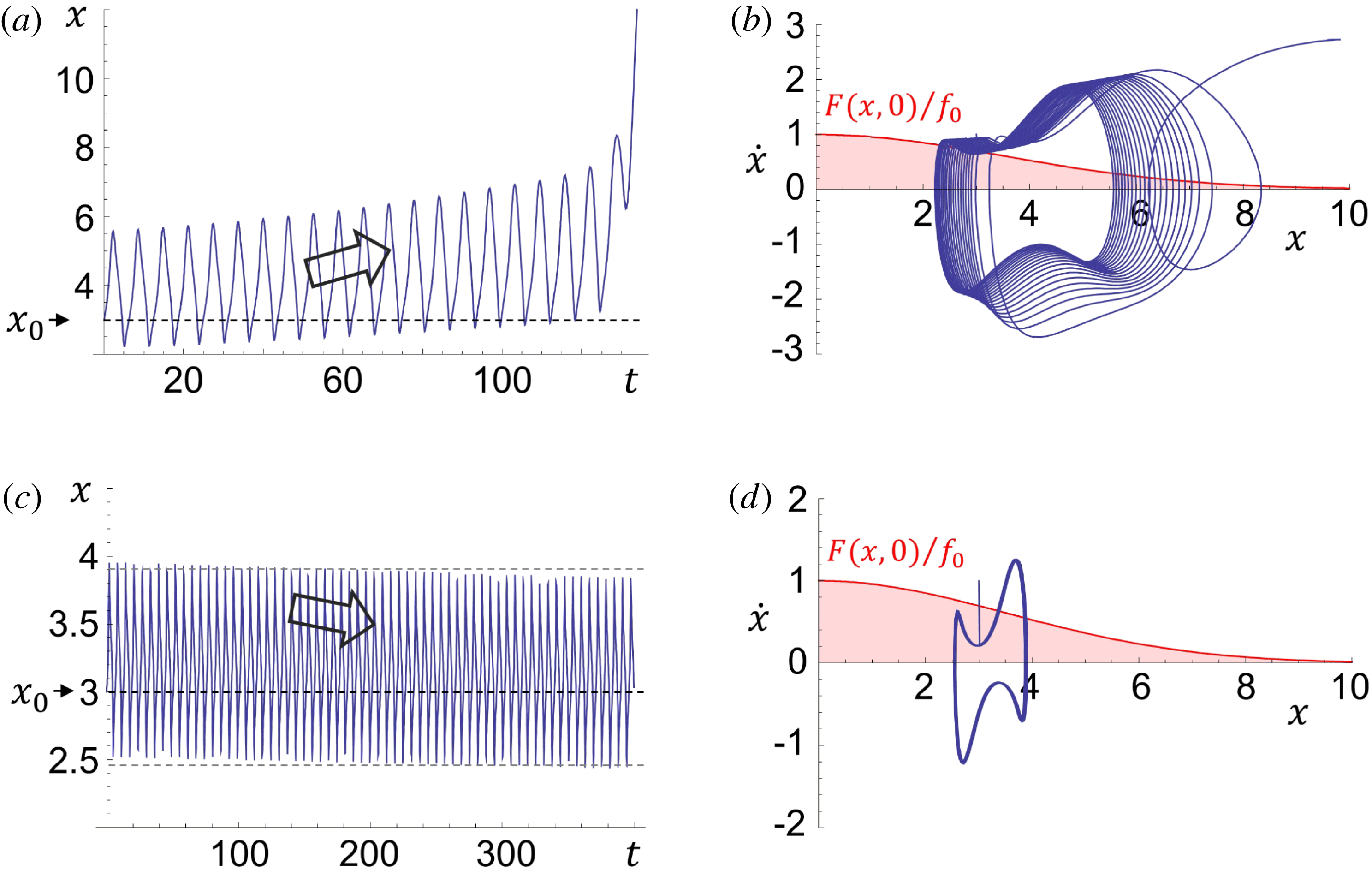
On a trajectory corresponding to a quasi-periodic particle motion seen in figure 10, the particle feels an almost constant driving force. This situation can be described in the approximation
 $$\begin{eqnarray}F(x,t)=f_{0}\cos \unicode[STIX]{x1D714}t,\quad \unicode[STIX]{x1D705}=\unicode[STIX]{x1D708}f_{0}^{2}\cos ^{2}\unicode[STIX]{x1D714}t.\end{eqnarray}$$
Substituting this driving force and friction coefficient into (4.1), we change variables to
 $(\unicode[STIX]{x1D70F},y(\unicode[STIX]{x1D70F}))$
,
$(\unicode[STIX]{x1D70F},y(\unicode[STIX]{x1D70F}))$
,
 $t=\unicode[STIX]{x1D70F}/\unicode[STIX]{x1D714}$
,
$t=\unicode[STIX]{x1D70F}/\unicode[STIX]{x1D714}$
,
 $x(t)=(f_{0}/\unicode[STIX]{x1D714}^{2})y(\unicode[STIX]{x1D70F})$
and introduce the constant
$x(t)=(f_{0}/\unicode[STIX]{x1D714}^{2})y(\unicode[STIX]{x1D70F})$
and introduce the constant
 $$\begin{eqnarray}\unicode[STIX]{x1D70E}=\unicode[STIX]{x1D708}f_{0}^{2}/\unicode[STIX]{x1D714}.\end{eqnarray}$$
Thus, we obtain
 $$\begin{eqnarray}y^{\prime \prime }(\unicode[STIX]{x1D70F})+\unicode[STIX]{x1D70E}\cos ^{2}(\unicode[STIX]{x1D70F})y^{\prime }(\unicode[STIX]{x1D70F})=\cos \unicode[STIX]{x1D70F}.\end{eqnarray}$$
Here a prime denotes a differentiation with respect to the variable
 $\unicode[STIX]{x1D70F}$
. Using (4.9) and the generating function for the modified Bessel functions of the first kind,
$\unicode[STIX]{x1D70F}$
. Using (4.9) and the generating function for the modified Bessel functions of the first kind,
 $I_{k}$
, one can cast the general solution to (4.18) in the form
$I_{k}$
, one can cast the general solution to (4.18) in the form
 $$\begin{eqnarray}y^{\prime }(\unicode[STIX]{x1D70F})=\exp \left(-\frac{\unicode[STIX]{x1D70E}\unicode[STIX]{x1D70F}}{2}-\frac{\unicode[STIX]{x1D70E}}{4}\sin (2\unicode[STIX]{x1D70F})\right)[y^{\prime }(0)-Y_{LC}(0)]+Y_{LC}(\unicode[STIX]{x1D70F}),\end{eqnarray}$$
where the function
 $Y_{LC}(\unicode[STIX]{x1D70F})$
is given by
$Y_{LC}(\unicode[STIX]{x1D70F})$
is given by
 $$\begin{eqnarray}\displaystyle Y_{LC}(\unicode[STIX]{x1D70F}) & = & \displaystyle \exp \left(-\frac{\unicode[STIX]{x1D70E}}{4}\sin (2\unicode[STIX]{x1D70F})\right)\mathop{\sum }_{k=-\infty }^{\infty }(-\text{i})^{k+1}I_{k}\left(\frac{\unicode[STIX]{x1D70E}}{4}\right)\nonumber\\ \displaystyle & & \displaystyle \times \left\{\frac{\exp [\text{i}(2k-1)\unicode[STIX]{x1D70F}]}{4k-2-\text{i}\unicode[STIX]{x1D70E}}+\frac{\exp [\text{i}(2k+1)\unicode[STIX]{x1D70F}]}{4k+2-\text{i}\unicode[STIX]{x1D70E}}\right\}.\end{eqnarray}$$
As one can see, any solution at
 $\unicode[STIX]{x1D70F}\rightarrow \infty$
tends to the limit cycle described by the function
$\unicode[STIX]{x1D70F}\rightarrow \infty$
tends to the limit cycle described by the function
 $Y_{LC}$
and determined by the constant
$Y_{LC}$
and determined by the constant
 $y^{\prime }(0)=Y_{LC}(0)$
.
$y^{\prime }(0)=Y_{LC}(0)$
.
The function describing the limit cycle, (4.20), can be represented as a Fourier series in terms of odd harmonics of the driving force frequency
 $$\begin{eqnarray}\displaystyle & \displaystyle Y_{LC}(\unicode[STIX]{x1D70F})=\mathop{\sum }_{n=1}^{\infty }[\exp (\text{i}(2n-1)\unicode[STIX]{x1D70F})C_{n}(\unicode[STIX]{x1D70E})+\exp (-\text{i}(2n-1)\unicode[STIX]{x1D70F})C_{1-n}(\unicode[STIX]{x1D70E})] & \displaystyle\end{eqnarray}$$
with
 $$\begin{eqnarray}C_{n}(\unicode[STIX]{x1D70E})=\text{i}^{n}\mathop{\sum }_{k=-\infty }^{\infty }\frac{(-1)^{k+1}}{4k+2-\text{i}\unicode[STIX]{x1D70E}}\left[I_{k}\left(\frac{\unicode[STIX]{x1D70E}}{4}\right)-\text{i}I_{k+1}\left(\frac{\unicode[STIX]{x1D70E}}{4}\right)\right]I_{k+1-n}\left(\frac{\unicode[STIX]{x1D70E}}{4}\right).\end{eqnarray}$$
This gives the spectrum of the limit cycle trajectory. For the particle velocity (corresponding to
 $y^{\prime }(\unicode[STIX]{x1D70F})$
), the spectral density is
$y^{\prime }(\unicode[STIX]{x1D70F})$
), the spectral density is
 $|2C_{n}(\unicode[STIX]{x1D70E})|^{2}$
, figure 11.
$|2C_{n}(\unicode[STIX]{x1D70E})|^{2}$
, figure 11.
The spectral density of the particle velocity for several harmonics of the driving force frequency as a function of the friction parameter
 $\unicode[STIX]{x1D70E}$
.
$\unicode[STIX]{x1D70E}$
.
We believe that the approach formulated above towards dissipative stabilization of nonlinear dynamics systems will be useful for applications well beyond the framework of laser–matter interaction physics, remembering a saying of William Thomson (Lord Kelvin) ‘I never satisfy myself until I can make a mechanical model of a thing’ (see Thomson Reference Thomson1884).
5 Regular and chaotic electron motion in three s- and p-polarized colliding laser pulses
5.1 EM field configuration
Let us consider three s(p)-polarized waves, in which the
 $z$
-component of the electric (magnetic) field is given by
$z$
-component of the electric (magnetic) field is given by
 $$\begin{eqnarray}\binom{E_{z}}{B_{z}}=-\frac{1}{\sqrt{3}}\binom{E_{0}}{B_{0}}\left\{\sin \left[\unicode[STIX]{x1D714}_{0}\left(t+\frac{y}{c}\right)\right]+2\sin \left[\unicode[STIX]{x1D714}_{0}\left(t-\frac{y}{2c}\right)\right]\cos \left(\unicode[STIX]{x1D714}_{0}\frac{\sqrt{3}x}{2c}\right)\right\}.\end{eqnarray}$$
The
 $x$
and
$x$
and
 $y$
components of the magnetic (electric) field of the s(p)-polarized wave are
$y$
components of the magnetic (electric) field of the s(p)-polarized wave are
 $$\begin{eqnarray}\binom{B_{x}}{E_{x}}=\frac{1}{\sqrt{3}}\binom{E_{0}}{-B_{0}}\left\{-\sin \left[\unicode[STIX]{x1D714}_{0}\left(t+\frac{y}{c}\right)\right]+\sin \left[\unicode[STIX]{x1D714}_{0}\left(t-\frac{y}{2c}\right)\right]\cos \left(\unicode[STIX]{x1D714}_{0}\frac{\sqrt{3}x}{2c}\right)\right\}\end{eqnarray}$$
and
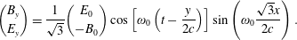 $$\begin{eqnarray}\binom{B_{y}}{E_{y}}=\frac{1}{\sqrt{3}}\binom{E_{0}}{-B_{0}}\cos \left[\unicode[STIX]{x1D714}_{0}\left(t-\frac{y}{2c}\right)\right]\sin \left(\unicode[STIX]{x1D714}_{0}\frac{\sqrt{3}x}{2c}\right).\end{eqnarray}$$
Wave vectors of three colliding waves.
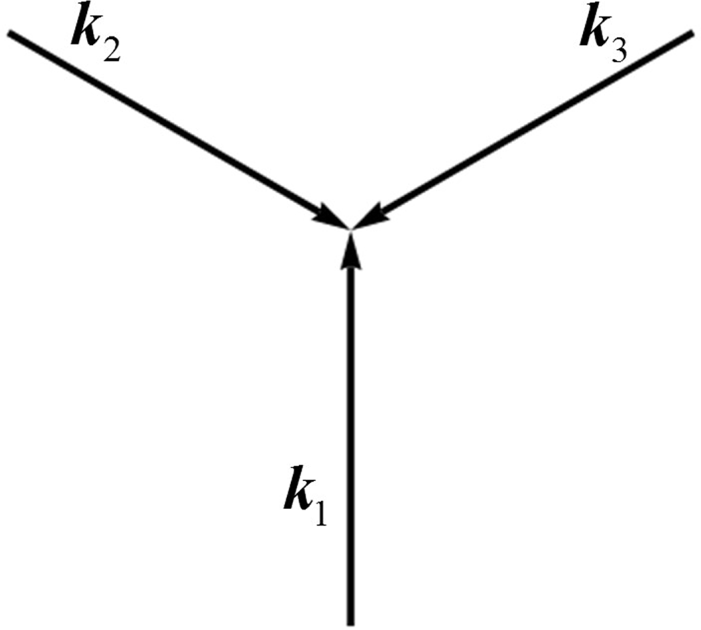
The wave orientation is illustrated in figure 12. As an example in figure 13(a) we show the magnetic (electric) field
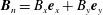 $\boldsymbol{B}_{n}=B_{x}\boldsymbol{e}_{x}+B_{y}\boldsymbol{e}_{y}$
(
$\boldsymbol{B}_{n}=B_{x}\boldsymbol{e}_{x}+B_{y}\boldsymbol{e}_{y}$
(
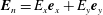 $\boldsymbol{E}_{n}=E_{x}\boldsymbol{e}_{x}+E_{y}\boldsymbol{e}_{y}$
) and in figure 13(b) the isocontours of the electric (magnetic) field
$\boldsymbol{E}_{n}=E_{x}\boldsymbol{e}_{x}+E_{y}\boldsymbol{e}_{y}$
) and in figure 13(b) the isocontours of the electric (magnetic) field
 $E_{z}$
(
$E_{z}$
(
 $B_{z}$
) in the
$B_{z}$
) in the
 $(x,y)$
plane at time
$(x,y)$
plane at time
 $t=\unicode[STIX]{x03C0}/4$
for the case of three colliding s-polarized (p-polarized) EM waves.
$t=\unicode[STIX]{x03C0}/4$
for the case of three colliding s-polarized (p-polarized) EM waves.
Three s-polarized (p-polarized) EM waves: (a) magnetic (electric) field; (b) isocontours of the electric (magnetic) field in the
 $(x,y)$
plane at time
$(x,y)$
plane at time
 $t=\unicode[STIX]{x03C0}/4$
.
$t=\unicode[STIX]{x03C0}/4$
.
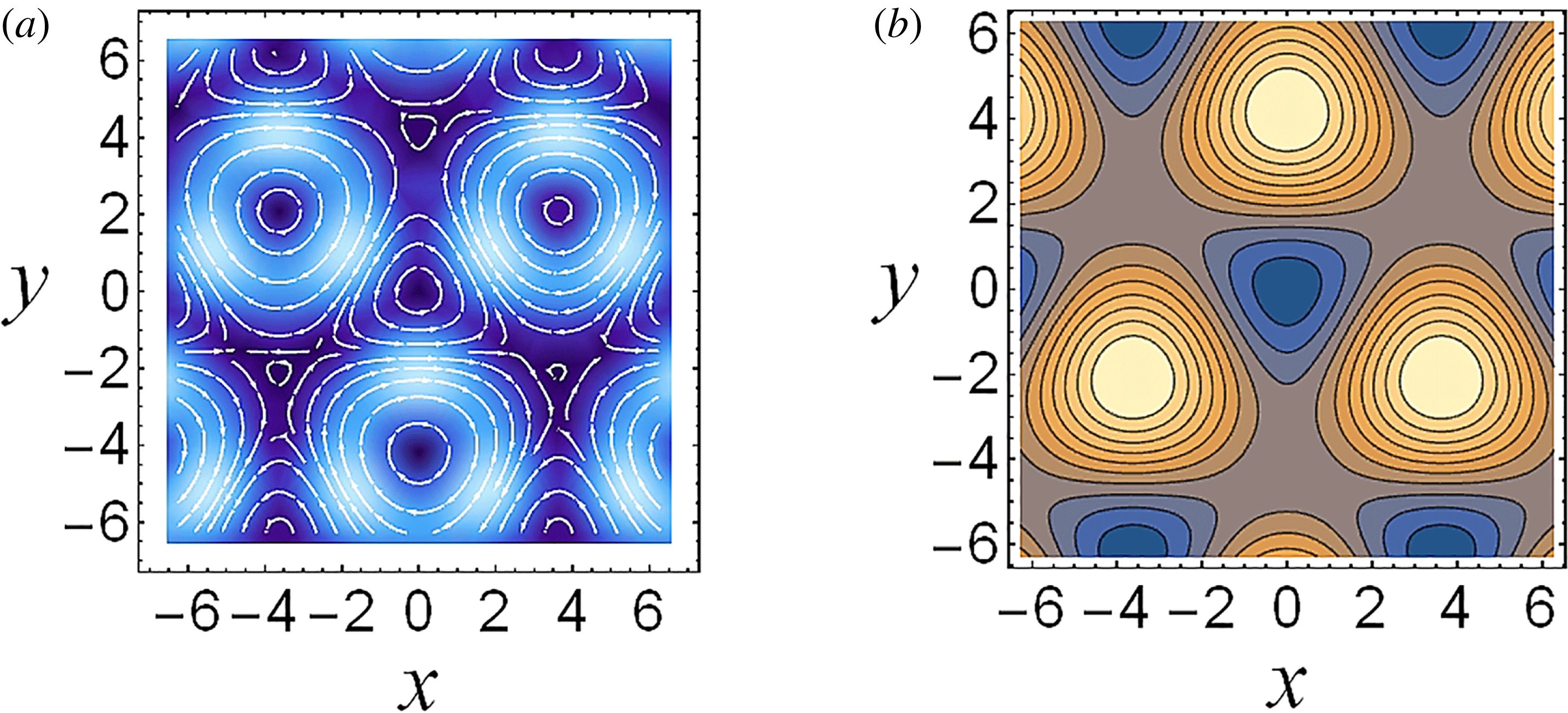
5.2 Electron interaction with three s-polarized EM waves
5.2.1 Particular solutions
Due to the symmetry of the EM field given by (5.2), (5.3), there are particular solutions of the equations of motion, when the particle moves straight in the
 $(x,y)$
plane along the direction of one of the waves propagation. If we let
$(x,y)$
plane along the direction of one of the waves propagation. If we let
 $x=0$
in (5.2), (5.3), the electromagnetic field formally corresponds to a superposition of two EM waves one of which propagates with the velocity equal to
$x=0$
in (5.2), (5.3), the electromagnetic field formally corresponds to a superposition of two EM waves one of which propagates with the velocity equal to
 $-c$
and another has the velocity
$-c$
and another has the velocity
 $2c$
.
$2c$
.
The integration of the equations of electron motion yields the particle trajectories presented in figure 14 for initial conditions:
 $x(0)=0$
,
$x(0)=0$
,
 $y(0)=0.05$
,
$y(0)=0.05$
,
 $z(0)=0$
,
$z(0)=0$
,
 $p_{x}(0)=0$
,
$p_{x}(0)=0$
,
 $p_{y}(0)=0$
,
$p_{y}(0)=0$
,
 $p_{z}(0)=0$
. The normalized electromagnetic field amplitude is
$p_{z}(0)=0$
. The normalized electromagnetic field amplitude is
 $a_{0}=436$
(each of the colliding waves has the amplitude equal to
$a_{0}=436$
(each of the colliding waves has the amplitude equal to
 $a_{0}/3$
), the dissipation parameter is
$a_{0}/3$
), the dissipation parameter is
 $\unicode[STIX]{x1D700}_{rad}=1.2\times 10^{-8}$
and the normalized critical QED field is
$\unicode[STIX]{x1D700}_{rad}=1.2\times 10^{-8}$
and the normalized critical QED field is
 $a_{S}=4\times 10^{5}$
. The electron trajectory in the
$a_{S}=4\times 10^{5}$
. The electron trajectory in the
 $(y,z)$
plane plotted in figure 14(a) and the trajectory in the phase
$(y,z)$
plane plotted in figure 14(a) and the trajectory in the phase
 $(y,p_{z})$
plane shown in figure 14(b) look similar to the trajectories presented in figure 2(a,b). The particle is trapped for a finite time within the EM field period performing relatively small-scale oscillations. Then, after some time it over-leaps to the next EM field period. This is also clearly seen in figure 14(c), where its
$(y,p_{z})$
plane shown in figure 14(b) look similar to the trajectories presented in figure 2(a,b). The particle is trapped for a finite time within the EM field period performing relatively small-scale oscillations. Then, after some time it over-leaps to the next EM field period. This is also clearly seen in figure 14(c), where its
 $y$
-coordinate is plotted versus time. From the Poincaré sections in figure 14(d), which show the particle positions in the phase plane
$y$
-coordinate is plotted versus time. From the Poincaré sections in figure 14(d), which show the particle positions in the phase plane
 $(p_{z},p_{y})$
at discrete times with the time step equal to the period of the driving force, we may see that this process is stochastic. The particle over-leaping from one field period to another with small-scale oscillations in between (see figures 2, 3 and 14) may be interpreted in terms of Lévy flights (Lévy Reference Lévy1954; Metzler & Klafter Reference Metzler and Klafter2000; Zaslavsky Reference Zaslavsky2002; Metzler et al.
Reference Metzler, Chechkin, Gonchar and Klafter2007).
$(p_{z},p_{y})$
at discrete times with the time step equal to the period of the driving force, we may see that this process is stochastic. The particle over-leaping from one field period to another with small-scale oscillations in between (see figures 2, 3 and 14) may be interpreted in terms of Lévy flights (Lévy Reference Lévy1954; Metzler & Klafter Reference Metzler and Klafter2000; Zaslavsky Reference Zaslavsky2002; Metzler et al.
Reference Metzler, Chechkin, Gonchar and Klafter2007).
(a) Electron trajectory in the
 $(y,z)$
plane for initial conditions:
$(y,z)$
plane for initial conditions:
 $x(0)=0$
,
$x(0)=0$
,
 $y(0)=0.05$
,
$y(0)=0.05$
,
 $z(0)=0$
,
$z(0)=0$
,
 $p_{x}(0)=0$
,
$p_{x}(0)=0$
,
 $p_{y}(0)=0$
,
$p_{y}(0)=0$
,
 $p_{z}(0)=0$
. (b) Trajectory in the phase
$p_{z}(0)=0$
. (b) Trajectory in the phase
 $(y,p_{z})$
plane; (c) electron
$(y,p_{z})$
plane; (c) electron
 $y$
-coordinate versus time; (d) the Poincaré sections showing the particle positions in the phase plane
$y$
-coordinate versus time; (d) the Poincaré sections showing the particle positions in the phase plane
 $(p_{z},p_{y})$
at discrete times with the time step equal to the period of the driving force. The electromagnetic field amplitude is
$(p_{z},p_{y})$
at discrete times with the time step equal to the period of the driving force. The electromagnetic field amplitude is
 $a_{0}=436$
, the dissipation parameter is
$a_{0}=436$
, the dissipation parameter is
 $\unicode[STIX]{x1D700}_{rad}=1.2\times 10^{-8}$
and the normalized critical QED field is
$\unicode[STIX]{x1D700}_{rad}=1.2\times 10^{-8}$
and the normalized critical QED field is
 $a_{S}=4\times 10^{5}$
. The coordinates, time and momentum are measured in
$a_{S}=4\times 10^{5}$
. The coordinates, time and momentum are measured in
 $2\unicode[STIX]{x03C0}c/\unicode[STIX]{x1D714}$
,
$2\unicode[STIX]{x03C0}c/\unicode[STIX]{x1D714}$
,
 $2\unicode[STIX]{x03C0}/\unicode[STIX]{x1D714}$
and
$2\unicode[STIX]{x03C0}/\unicode[STIX]{x1D714}$
and
 $m_{e}c$
units.
$m_{e}c$
units.
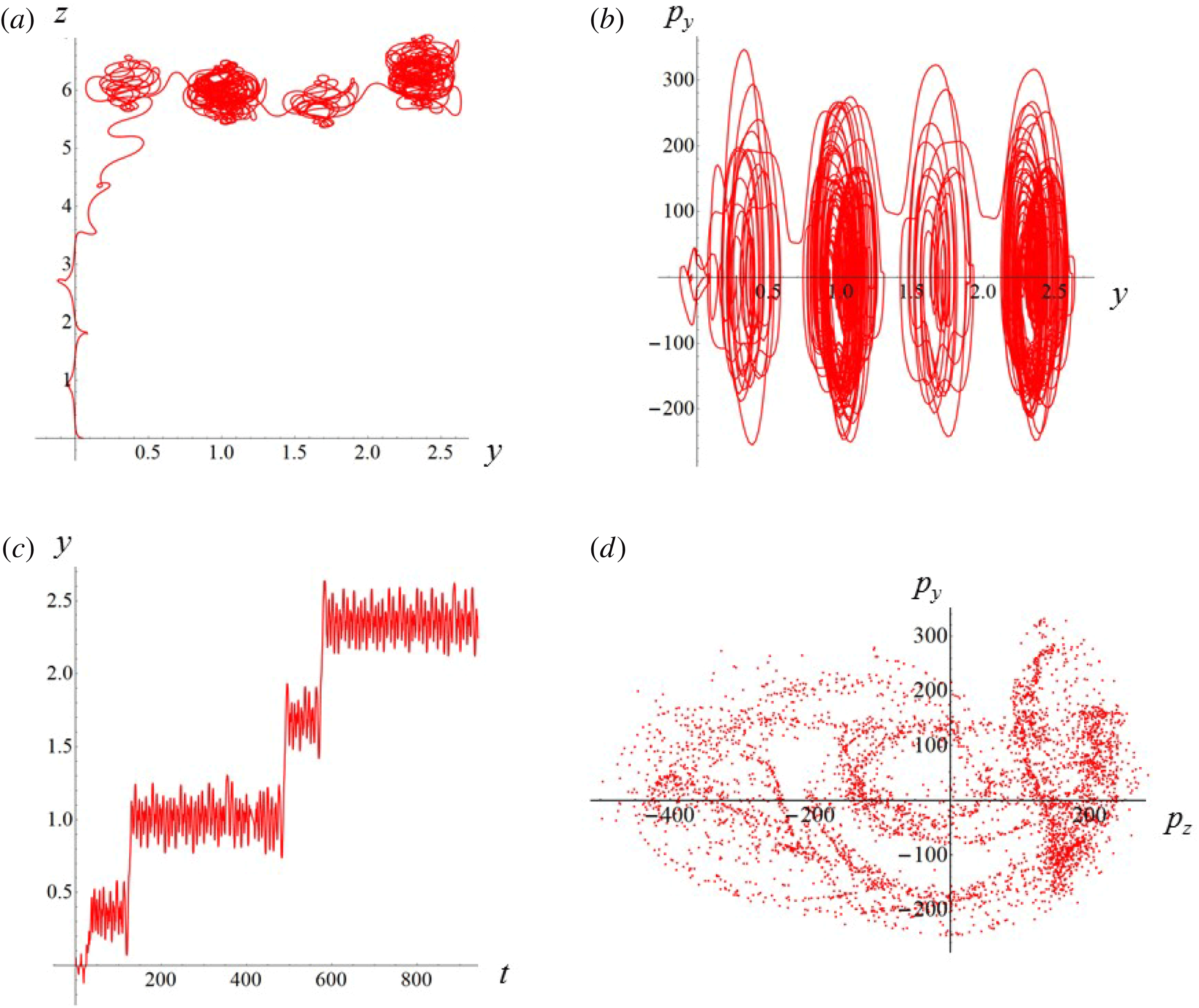
The case of high laser amplitude is presented in figure 15 for initial conditions:
 $x(0)=0$
,
$x(0)=0$
,
 $y(0)=-0.0001$
,
$y(0)=-0.0001$
,
 $z(0)=0$
,
$z(0)=0$
,
 $p_{x}(0)=0$
,
$p_{x}(0)=0$
,
 $p_{y}(0)=0$
,
$p_{y}(0)=0$
,
 $p_{z}(0)=0$
. The normalized electromagnetic field amplitude is
$p_{z}(0)=0$
. The normalized electromagnetic field amplitude is
 $a_{0}=4700$
(each of the colliding waves has the amplitude equal to
$a_{0}=4700$
(each of the colliding waves has the amplitude equal to
 $a_{0}/3$
), the dissipation parameter is
$a_{0}/3$
), the dissipation parameter is
 $\unicode[STIX]{x1D700}_{rad}=1.2\times 10^{-9}$
and the normalized critical QED field is
$\unicode[STIX]{x1D700}_{rad}=1.2\times 10^{-9}$
and the normalized critical QED field is
 $a_{S}=4\times 10^{6}$
. The electron trajectory in the
$a_{S}=4\times 10^{6}$
. The electron trajectory in the
 $(y,z)$
plane plotted in figure 15(a) and the trajectory in the phase
$(y,z)$
plane plotted in figure 15(a) and the trajectory in the phase
 $(y,p_{y})$
plane shown in figure 15(b) clearly demonstrate the particle trapping in the limit circle after an initial phase corresponding to the particle motion in the vicinity of the electric field node,
$(y,p_{y})$
plane shown in figure 15(b) clearly demonstrate the particle trapping in the limit circle after an initial phase corresponding to the particle motion in the vicinity of the electric field node,
 $y=0$
. Since the motion here is unstable, the particle leaves this region. This is also distinctly seen in figure 15(d) showing the electron trajectory in the
$y=0$
. Since the motion here is unstable, the particle leaves this region. This is also distinctly seen in figure 15(d) showing the electron trajectory in the
 $(p_{y},p_{z})$
plane. In the plane
$(p_{y},p_{z})$
plane. In the plane
 $(y,z)$
(figure 15
a) as we see, when the particle moves along the limit circle, its trajectory has the ‘figure eight’ form. It performs regular oscillations (see figure 15
c, where the particle coordinate
$(y,z)$
(figure 15
a) as we see, when the particle moves along the limit circle, its trajectory has the ‘figure eight’ form. It performs regular oscillations (see figure 15
c, where the particle coordinate
 $y$
is plotted versus time) with the double frequency for oscillations along the
$y$
is plotted versus time) with the double frequency for oscillations along the
 $y$
axis compared with the frequency of oscillation along the
$y$
axis compared with the frequency of oscillation along the
 $z$
axis.
$z$
axis.
(a) Electron trajectory in the
 $(y,z)$
plane for initial conditions:
$(y,z)$
plane for initial conditions:
 $x(0)=0$
,
$x(0)=0$
,
 $y(0)=-0.0001$
,
$y(0)=-0.0001$
,
 $z(0)=0$
,
$z(0)=0$
,
 $p_{x}(0)=0$
,
$p_{x}(0)=0$
,
 $p_{y}(0)=0$
,
$p_{y}(0)=0$
,
 $p_{z}(0)=0$
. (b) Trajectory in the phase plane
$p_{z}(0)=0$
. (b) Trajectory in the phase plane
 $(y,p_{y})$
; (c) electron
$(y,p_{y})$
; (c) electron
 $y$
-coordinate versus time; (d) electron trajectory in the
$y$
-coordinate versus time; (d) electron trajectory in the
 $(p_{y},p_{z})$
plane. The electromagnetic field amplitude is
$(p_{y},p_{z})$
plane. The electromagnetic field amplitude is
 $a_{0}=4700$
, the dissipation parameter is
$a_{0}=4700$
, the dissipation parameter is
 $\unicode[STIX]{x1D700}_{rad}=1.2\times 10^{-9}$
and the normalized critical QED field is
$\unicode[STIX]{x1D700}_{rad}=1.2\times 10^{-9}$
and the normalized critical QED field is
 $a_{S}=4\times 10^{6}$
. The coordinates, time and momentum are measured in
$a_{S}=4\times 10^{6}$
. The coordinates, time and momentum are measured in
 $2\unicode[STIX]{x03C0}c/\unicode[STIX]{x1D714}$
,
$2\unicode[STIX]{x03C0}c/\unicode[STIX]{x1D714}$
,
 $2\unicode[STIX]{x03C0}/\unicode[STIX]{x1D714}$
and
$2\unicode[STIX]{x03C0}/\unicode[STIX]{x1D714}$
and
 $m_{e}c$
units.
$m_{e}c$
units.
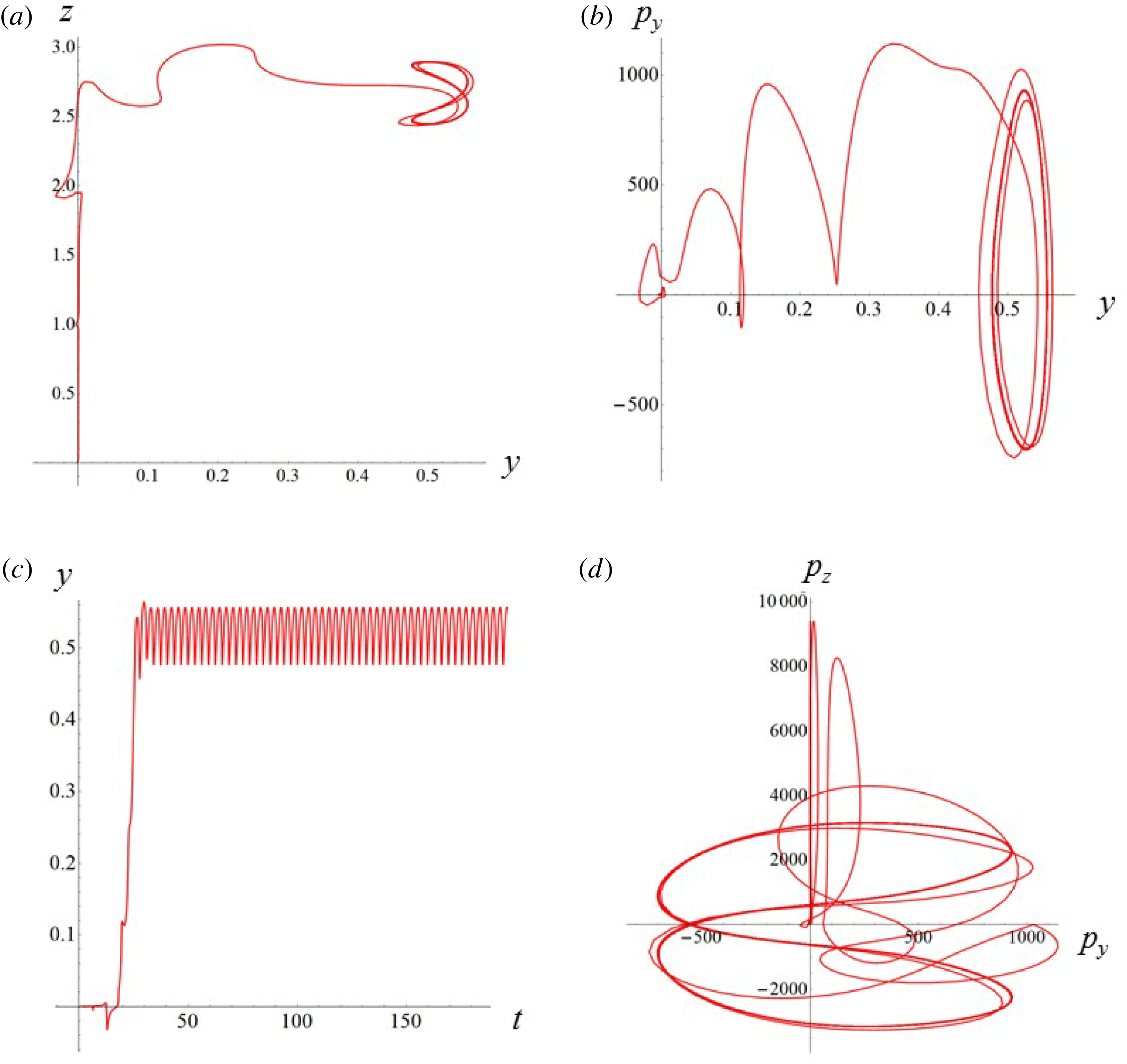
5.2.2 Random walk and regular patterns of the particle trajectories in the field of three 3 s-polarized EM waves
Results of the integration of the motion equations for the electron interacting with three 3 s-polarized EM waves in the limit of relatively low radiation intensity are presented in figure 16. Figure 16(a) shows 8 electron trajectories in the
 $(x,y)$
plane for initial conditions:
$(x,y)$
plane for initial conditions:
 $x(0)$
and
$x(0)$
and
 $y(0)$
are in the vicinity of the coordinate origin, and
$y(0)$
are in the vicinity of the coordinate origin, and
 $z(0)=0$
,
$z(0)=0$
,
 $p_{x}(0)=0$
,
$p_{x}(0)=0$
,
 $p_{y}(0)=0$
,
$p_{y}(0)=0$
,
 $p_{z}(0)=0$
. In figure 16(b) we plot a close up of the trajectories in the vicinity of the coordinate origin superimposed with the isocontours of the electromagnetic potential averaged over a half-period of the field oscillations. It is proportional to the ponderomotive potential in the high field amplitude limit,
$p_{z}(0)=0$
. In figure 16(b) we plot a close up of the trajectories in the vicinity of the coordinate origin superimposed with the isocontours of the electromagnetic potential averaged over a half-period of the field oscillations. It is proportional to the ponderomotive potential in the high field amplitude limit,
 $a_{0}\gg 1$
. As we see the typical trajectories are comprised of long range Lévy-flight-like excursions and short range rambling motion, which changes the direction of succeeding flight. The combination of the long range excursions and short range rambling is also seen in the dependence of the electron
$a_{0}\gg 1$
. As we see the typical trajectories are comprised of long range Lévy-flight-like excursions and short range rambling motion, which changes the direction of succeeding flight. The combination of the long range excursions and short range rambling is also seen in the dependence of the electron
 $y$
coordinate on time in figure 16(d). The corresponding particle trajectory in the
$y$
coordinate on time in figure 16(d). The corresponding particle trajectory in the
 $p_{x},p_{y},p_{z}$
momentum space for
$p_{x},p_{y},p_{z}$
momentum space for
 $x(0)=-0.125$
and
$x(0)=-0.125$
and
 $y(0)=0.125$
is presented in figure 16(c). What is remarkable is that during the Lévy-like flights the electron moves almost along one of the three waves propagation direction (compare figures 12 and 16
a). This stage of the particle motion can be described by the particular solution analysed above and illustrated in figure 14.
$y(0)=0.125$
is presented in figure 16(c). What is remarkable is that during the Lévy-like flights the electron moves almost along one of the three waves propagation direction (compare figures 12 and 16
a). This stage of the particle motion can be described by the particular solution analysed above and illustrated in figure 14.
(a) Eight electron trajectories in the
 $(x,y)$
plane for initial conditions:
$(x,y)$
plane for initial conditions:
 $x(0)$
and
$x(0)$
and
 $y(0)$
are in the vicinity of the coordinate origin, and
$y(0)$
are in the vicinity of the coordinate origin, and
 $z(0)=0$
,
$z(0)=0$
,
 $p_{x}(0)=0$
,
$p_{x}(0)=0$
,
 $p_{y}(0)=0$
,
$p_{y}(0)=0$
,
 $p_{z}(0)=0$
. (b) Close up of the trajectories in the vicinity of the coordinate origin. (c) Electron trajectory in the
$p_{z}(0)=0$
. (b) Close up of the trajectories in the vicinity of the coordinate origin. (c) Electron trajectory in the
 $p_{x},p_{y},p_{z}$
space for
$p_{x},p_{y},p_{z}$
space for
 $x(0)=-0.125$
and
$x(0)=-0.125$
and
 $y(0)=0.125$
. (d) Electron
$y(0)=0.125$
. (d) Electron
 $y$
coordinate versus time for
$y$
coordinate versus time for
 $x(0)=-0.125$
and
$x(0)=-0.125$
and
 $y(0)=0.125$
. The electromagnetic field amplitude is
$y(0)=0.125$
. The electromagnetic field amplitude is
 $a_{0}=756$
, the dissipation parameter is
$a_{0}=756$
, the dissipation parameter is
 $\unicode[STIX]{x1D700}_{rad}=1.2\times 10^{-8}$
and the normalized critical QED field is
$\unicode[STIX]{x1D700}_{rad}=1.2\times 10^{-8}$
and the normalized critical QED field is
 $a_{S}=4\times 10^{5}$
. The coordinates, time and momentum are measured in
$a_{S}=4\times 10^{5}$
. The coordinates, time and momentum are measured in
 $2\unicode[STIX]{x03C0}c/\unicode[STIX]{x1D714}$
,
$2\unicode[STIX]{x03C0}c/\unicode[STIX]{x1D714}$
,
 $2\unicode[STIX]{x03C0}/\unicode[STIX]{x1D714}$
and
$2\unicode[STIX]{x03C0}/\unicode[STIX]{x1D714}$
and
 $m_{e}c$
units.
$m_{e}c$
units.

(a) Ensemble of electron trajectories in the
 $(x,y)$
plane for initial conditions:
$(x,y)$
plane for initial conditions:
 $x(0)$
and
$x(0)$
and
 $y(0)$
are in the vicinity of the coordinate origin, and
$y(0)$
are in the vicinity of the coordinate origin, and
 $z(0)=0$
,
$z(0)=0$
,
 $p_{x}(0)=0$
,
$p_{x}(0)=0$
,
 $p_{y}(0)=0$
,
$p_{y}(0)=0$
,
 $p_{z}(0)=0$
. (b) Close up of the trajectories in the vicinity of the coordinate origin. (c) Electron trajectory in the
$p_{z}(0)=0$
. (b) Close up of the trajectories in the vicinity of the coordinate origin. (c) Electron trajectory in the
 $p_{x},p_{y},p_{z}$
space for
$p_{x},p_{y},p_{z}$
space for
 $x(0)=-0.125$
and
$x(0)=-0.125$
and
 $y(0)=0.125$
. (d) Electron
$y(0)=0.125$
. (d) Electron
 $y$
coordinate versus time for
$y$
coordinate versus time for
 $x(0)=-0.001$
and
$x(0)=-0.001$
and
 $y(0)=-0.001$
. (e) The Poincaŕe sections: the particle positions in the phase plane
$y(0)=-0.001$
. (e) The Poincaŕe sections: the particle positions in the phase plane
 $(p_{x},p_{y})$
at discrete times with the time step equal to the period of the driving force. The electromagnetic field amplitude is
$(p_{x},p_{y})$
at discrete times with the time step equal to the period of the driving force. The electromagnetic field amplitude is
 $a_{0}=4764$
, the dissipation parameter is
$a_{0}=4764$
, the dissipation parameter is
 $\unicode[STIX]{x1D700}_{rad}=6\times 10^{-9}$
and the normalized critical QED field is
$\unicode[STIX]{x1D700}_{rad}=6\times 10^{-9}$
and the normalized critical QED field is
 $a_{S}=8\times 10^{5}$
. The coordinates, time and momentum are measured in
$a_{S}=8\times 10^{5}$
. The coordinates, time and momentum are measured in
 $2\unicode[STIX]{x03C0}c/\unicode[STIX]{x1D714}$
,
$2\unicode[STIX]{x03C0}c/\unicode[STIX]{x1D714}$
,
 $2\unicode[STIX]{x03C0}/\unicode[STIX]{x1D714}$
and
$2\unicode[STIX]{x03C0}/\unicode[STIX]{x1D714}$
and
 $m_{e}c$
units. The integration time equals
$m_{e}c$
units. The integration time equals
 $200\times 2\unicode[STIX]{x03C0}/\unicode[STIX]{x1D714}$
.
$200\times 2\unicode[STIX]{x03C0}/\unicode[STIX]{x1D714}$
.
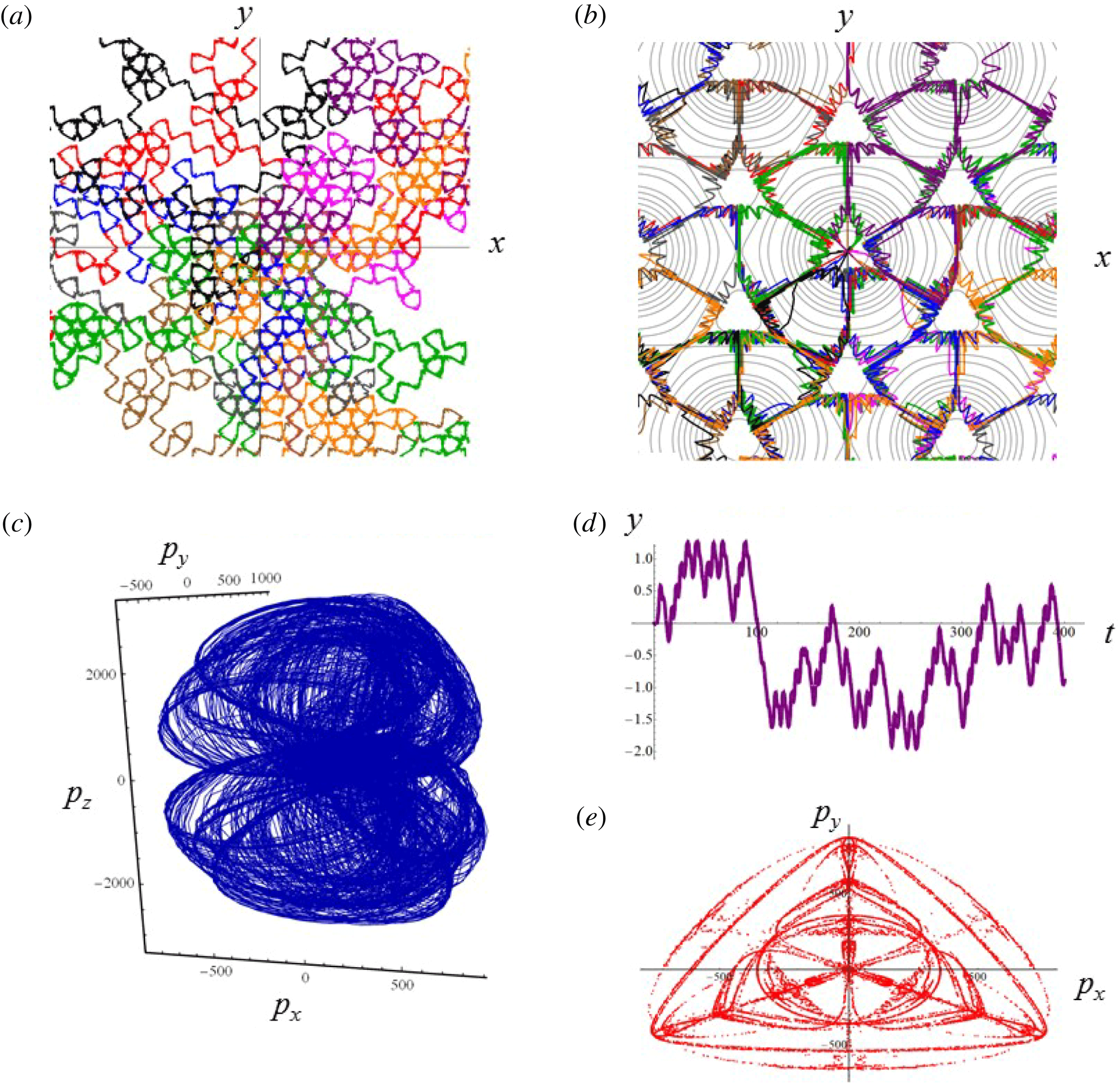
Qualitatively different patterns formed by the trajectories of particles interacting with the field of three 3 s-polarized EM waves are observed in the high intensity and low frequency limit. These patterns are shown in figure 17(a) and in figure 17(b) presenting a close up of the trajectories in the vicinity of the coordinate origin, where the trajectories in the
 $(x,y)$
plane of an electron ensemble make a tracery strikingly remeniscent of parquetry or window frost. Either an individual trajectory or the ensemble appears to be confined in the lower measure sub-domain periodic in the
$(x,y)$
plane of an electron ensemble make a tracery strikingly remeniscent of parquetry or window frost. Either an individual trajectory or the ensemble appears to be confined in the lower measure sub-domain periodic in the
 $x$
and
$x$
and
 $y$
directions. In figure 17(c) the electron trajectory in the
$y$
directions. In figure 17(c) the electron trajectory in the
 $p_{x},p_{y},p_{z}$
momentum space for
$p_{x},p_{y},p_{z}$
momentum space for
 $x(0)=-0.125$
and
$x(0)=-0.125$
and
 $y(0)=0.125$
demonstrates that the particle energy remains finite. The electron
$y(0)=0.125$
demonstrates that the particle energy remains finite. The electron
 $y$
coordinate dependence on time for
$y$
coordinate dependence on time for
 $x(0)=-0.001$
and
$x(0)=-0.001$
and
 $y(0)=-0.001$
plotted in figure 17(c) shows that the particle motion is comprised of relatively long over-leaps interlaced with small-scale oscillations. In figure 17(e) we present the corresponding Poincaŕe sections, i.e. we plot the particle positions in the phase plane
$y(0)=-0.001$
plotted in figure 17(c) shows that the particle motion is comprised of relatively long over-leaps interlaced with small-scale oscillations. In figure 17(e) we present the corresponding Poincaŕe sections, i.e. we plot the particle positions in the phase plane
 $(p_{x},p_{y})$
at discrete times with the time step equal to the period of the driving force. The Poincaŕe sections, in this case, indicate that the particle motion is pretty regular. Here the parameters of the EM field and of the electrons are as follows. The electromagnetic field amplitude is
$(p_{x},p_{y})$
at discrete times with the time step equal to the period of the driving force. The Poincaŕe sections, in this case, indicate that the particle motion is pretty regular. Here the parameters of the EM field and of the electrons are as follows. The electromagnetic field amplitude is
 $a_{0}=4764$
(the amplitude of each colliding wave is equal to 1588), the dissipation parameter is
$a_{0}=4764$
(the amplitude of each colliding wave is equal to 1588), the dissipation parameter is
 $\unicode[STIX]{x1D700}_{rad}=6\times 10^{-9}$
and the normalized critical QED field is
$\unicode[STIX]{x1D700}_{rad}=6\times 10^{-9}$
and the normalized critical QED field is
 $a_{S}=8\times 10^{5}$
, which corresponds to the wave frequency a factor two smaller than in the case shown in figure 16. The integration time equals
$a_{S}=8\times 10^{5}$
, which corresponds to the wave frequency a factor two smaller than in the case shown in figure 16. The integration time equals
 $200\times 2\unicode[STIX]{x03C0}/\unicode[STIX]{x1D714}$
.
$200\times 2\unicode[STIX]{x03C0}/\unicode[STIX]{x1D714}$
.
5.2.3 Ergodization or not?
The attractor trajectory pattern in figure 17(a,b) is made by an ensemble of electrons. The single electron trajectory shown in figure 18 demonstrates that, having been moving for a long enough time, it could cover the whole attractor. In view of this, there are two questions. The first one being whether there is an analogy of the ergodic hypothesis saying that over long periods of time, the time spent in some region of the attractor is proportional to the attractor measure? The second one being whether there is an analogy of the Poincaré recurrence theorem (for details see Arnol’d Reference Arnol’d1989) saying that the particle, after a sufficiently long but finite time, returns to a point very close to the initial point? A similar question occurs in the case of the particle random walk regarding whether the results of the well-known random walk theory (Kac Reference Kac1961) can be used in our case. In both the regular and stochastic regimes the methods developed in turbulence theory (see Mathur et al. Reference Mathur, Haller, Peacock, Ruppert-Felsot and Swinney2007; Peacock & Haller Reference Peacock and Haller2013) can be used for analysing and identifying the attractors and repelling trajectories.
Trajectory of the electron migrating over a long time in the
 $(x,y)$
plane.
$(x,y)$
plane.
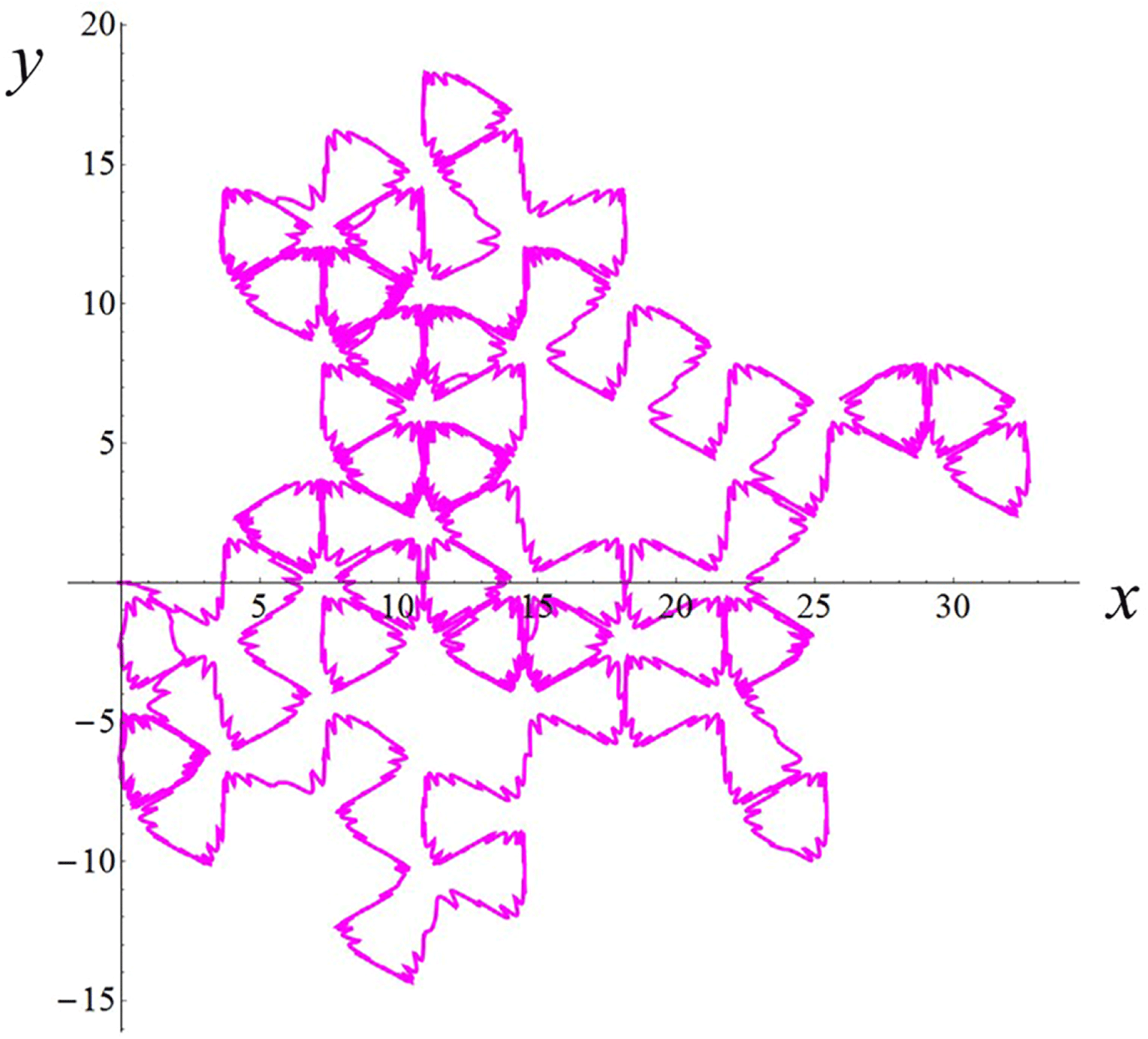
5.3 Electron interaction with three p-polarized EM waves
In the case of three p-polarized EM waves the EM configuration is described by (5.1)–(5.3). As in the s-polarization case, in the limit of relatively low EM wave intensity the electron performs the random walk motion comprised of short scale-length oscillations interleaved by long scale-length Lévy-like flights. An example of such the trajectory is shown in figure 19(a) for the EM field amplitude of
 $a_{0}=4764$
, the dissipation parameter of
$a_{0}=4764$
, the dissipation parameter of
 $\unicode[STIX]{x1D700}_{rad}=6\times 10^{-9}$
and the normalized critical QED field of
$\unicode[STIX]{x1D700}_{rad}=6\times 10^{-9}$
and the normalized critical QED field of
 $a_{S}=8\times 10^{5}$
. For the high intensity EM wave case the electrons migrate along the paths confined in narrow valleys, as can be seen in figure 19(b), where the ensemble of the electron trajectories is plotted for the EM field amplitude of
$a_{S}=8\times 10^{5}$
. For the high intensity EM wave case the electrons migrate along the paths confined in narrow valleys, as can be seen in figure 19(b), where the ensemble of the electron trajectories is plotted for the EM field amplitude of
 $7.2\times 10^{3}$
, the dissipation parameter of
$7.2\times 10^{3}$
, the dissipation parameter of
 $\unicode[STIX]{x1D700}_{rad}=1.2\times 10^{-8}$
and the normalized critical QED field of
$\unicode[STIX]{x1D700}_{rad}=1.2\times 10^{-8}$
and the normalized critical QED field of
 $a_{S}=4.1\times 10^{5}$
.
$a_{S}=4.1\times 10^{5}$
.
(a) Ensemble of electron trajectories in the
 $(x,y)$
plane for initial conditions:
$(x,y)$
plane for initial conditions:
 $x(0)$
and
$x(0)$
and
 $y(0)$
are in the vicinity of the coordinate origin, and
$y(0)$
are in the vicinity of the coordinate origin, and
 $z(0)=0$
,
$z(0)=0$
,
 $p_{x}(0)=0$
,
$p_{x}(0)=0$
,
 $p_{y}(0)=0$
,
$p_{y}(0)=0$
,
 $p_{z}(0)=0$
. (b) Electron trajectories in the
$p_{z}(0)=0$
. (b) Electron trajectories in the
 $(p_{x},p_{y})$
plane. (c) The Poincaŕe sections: the particle positions in the phase plane
$(p_{x},p_{y})$
plane. (c) The Poincaŕe sections: the particle positions in the phase plane
 $(p_{x},p_{y})$
at discrete times with the time step equal to the period of the driving force. The electromagnetic field amplitude is
$(p_{x},p_{y})$
at discrete times with the time step equal to the period of the driving force. The electromagnetic field amplitude is
 $a_{0}=1383$
, the dissipation parameter is
$a_{0}=1383$
, the dissipation parameter is
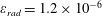 $\unicode[STIX]{x1D700}_{rad}=1.2\times 10^{-6}$
and the normalized critical QED field is
$\unicode[STIX]{x1D700}_{rad}=1.2\times 10^{-6}$
and the normalized critical QED field is
 $a_{S}=4.1\times 10^{5}$
. (d) Ensemble of electron trajectories in the
$a_{S}=4.1\times 10^{5}$
. (d) Ensemble of electron trajectories in the
 $(x,y)$
plane for initial conditions:
$(x,y)$
plane for initial conditions:
 $x(0)$
and
$x(0)$
and
 $y(0)$
are in the vicinity of the coordinate origin, and
$y(0)$
are in the vicinity of the coordinate origin, and
 $z(0)=0$
,
$z(0)=0$
,
 $p_{x}(0)=0$
,
$p_{x}(0)=0$
,
 $p_{y}(0)=0$
,
$p_{y}(0)=0$
,
 $p_{z}(0)=0$
. (e) Electron trajectories in the
$p_{z}(0)=0$
. (e) Electron trajectories in the
 $(p_{x},p_{y})$
plane. (f) The Poincaŕe sections: the particle positions in the phase plane
$(p_{x},p_{y})$
plane. (f) The Poincaŕe sections: the particle positions in the phase plane
 $(p_{x},p_{y})$
at discrete times with the time step equal to the period of the driving force. The electromagnetic field amplitude is
$(p_{x},p_{y})$
at discrete times with the time step equal to the period of the driving force. The electromagnetic field amplitude is
 $a_{0}=7.2\times 10^{3}$
, the dissipation parameter is
$a_{0}=7.2\times 10^{3}$
, the dissipation parameter is
 $\unicode[STIX]{x1D700}_{rad}=1.2\times 10^{-8}$
and the normalized critical QED field is
$\unicode[STIX]{x1D700}_{rad}=1.2\times 10^{-8}$
and the normalized critical QED field is
 $a_{S}=4.1\times 10^{5}$
.
$a_{S}=4.1\times 10^{5}$
.
6 Electron dynamics in four s- and p-polarized colliding EM pulses
The orientation of four colliding waves is illustrated in figure 20. Figure 21(a) shows magnetic (electric) field and (b) isocontours of the electric (magnetic) field in the
 $(x,y)$
plane at time
$(x,y)$
plane at time
 $t=\unicode[STIX]{x03C0}/4$
of four s-polarized (p-polarized) colliding EM waves.
$t=\unicode[STIX]{x03C0}/4$
of four s-polarized (p-polarized) colliding EM waves.
Wave vectors of four colliding EM waves.
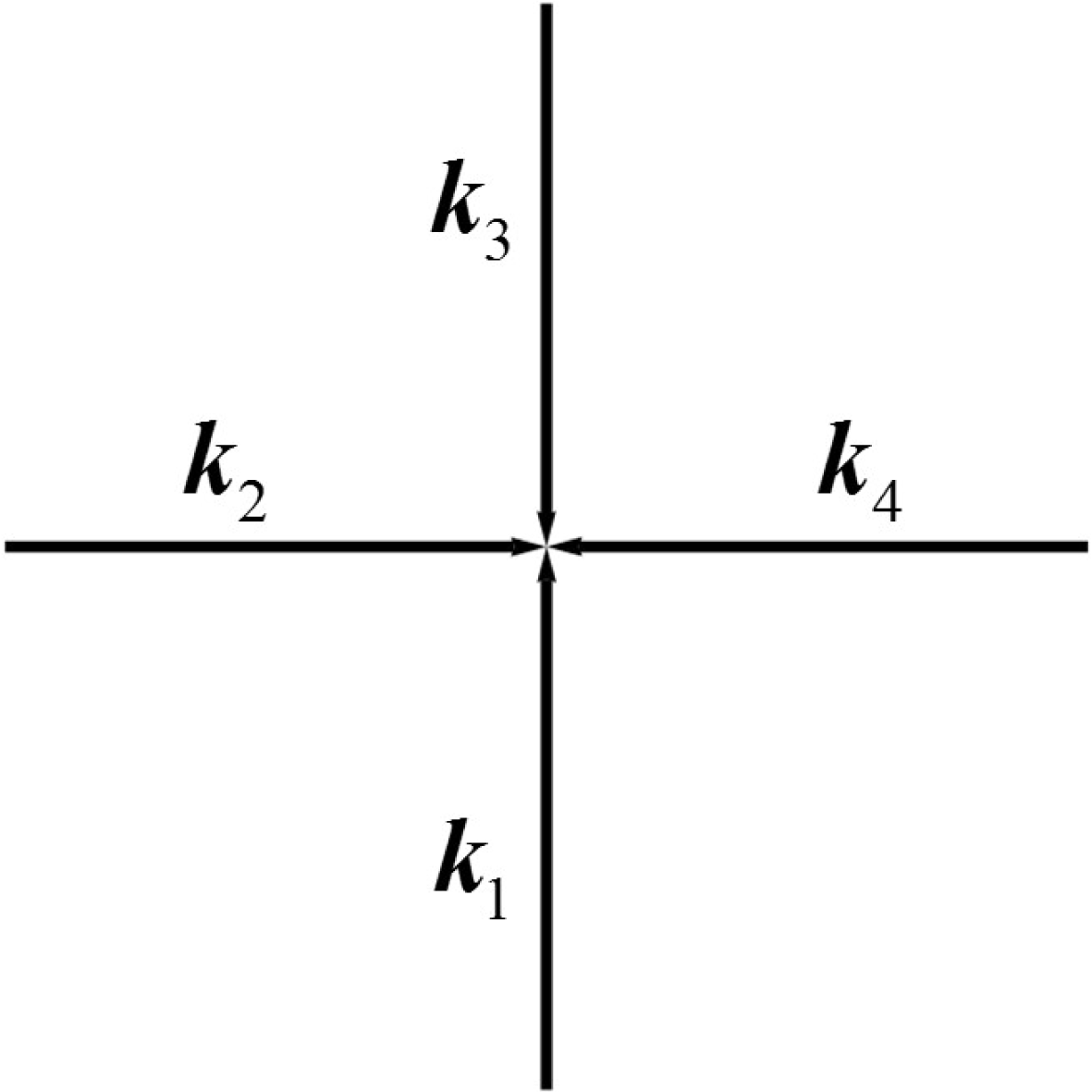
Four s-polarized (p-polarized) EM waves: (a) magnetic (electric) field; (b) isocontours of the electric (magnetic) field in the
 $(x,y)$
plane at time
$(x,y)$
plane at time
 $t=\unicode[STIX]{x03C0}/4$
.
$t=\unicode[STIX]{x03C0}/4$
.
6.1 S-polarized 4 colliding EM waves
6.1.1 EM field configuration
In the EM configuration of four colliding s(p)-polarized waves the
 $z$
-components of the electric (magnetic) field can be written
$z$
-components of the electric (magnetic) field can be written
 $$\begin{eqnarray}\left(\begin{array}{@{}c@{}}E_{z}\\ B_{z}\end{array}\right)=\left(\begin{array}{@{}c@{}}E_{0}\\ B_{0}\end{array}\right)2\sin (\unicode[STIX]{x1D714}_{0}t)\left[\cos \left(\unicode[STIX]{x1D714}_{0}\frac{x}{c}\right)+\cos \left(\unicode[STIX]{x1D714}_{0}\frac{y}{c}\right)\right].\end{eqnarray}$$
The
 $x$
and
$x$
and
 $y$
components of the magnetic (electric) field of the four colliding s(p)-polarized waves are given by
$y$
components of the magnetic (electric) field of the four colliding s(p)-polarized waves are given by
 $$\begin{eqnarray}\left(\begin{array}{@{}c@{}}B_{x}\\ E_{x}\end{array}\right)=\left(\begin{array}{@{}c@{}}-E_{0}\\ B_{0}\end{array}\right)2\cos (\unicode[STIX]{x1D714}_{0}t)\sin \left(\unicode[STIX]{x1D714}_{0}\frac{y}{c}\right)\end{eqnarray}$$
and
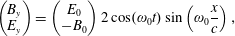 $$\begin{eqnarray}\left(\begin{array}{@{}c@{}}B_{y}\\ E_{y}\end{array}\right)=\left(\begin{array}{@{}c@{}}E_{0}\\ -B_{0}\end{array}\right)2\cos (\unicode[STIX]{x1D714}_{0}t)\sin \left(\unicode[STIX]{x1D714}_{0}\frac{x}{c}\right),\end{eqnarray}$$
respectively.
Electron trajectories in the case of the first type particular solution corresponding to the motion along the
 $y$
axis (at
$y$
axis (at
 $x=0$
) in the field of four colliding EM waves for
$x=0$
) in the field of four colliding EM waves for
 $\unicode[STIX]{x1D700}_{rad}=1.2\times 10^{-9}$
,
$\unicode[STIX]{x1D700}_{rad}=1.2\times 10^{-9}$
,
 $a_{S}=4\times 10^{6}$
,
$a_{S}=4\times 10^{6}$
,
 $a=94$
,
$a=94$
,
 $\unicode[STIX]{x1D714}=0.1$
for initial conditions:
$\unicode[STIX]{x1D714}=0.1$
for initial conditions:
 $y(0)=0.01$
,
$y(0)=0.01$
,
 $z(0)=0$
,
$z(0)=0$
,
 $p_{y}(0)=0$
,
$p_{y}(0)=0$
,
 $p_{z}(0)=0$
(red,
$p_{z}(0)=0$
(red,
 $-1$
);
$-1$
);
 $y(0)=0.23$
,
$y(0)=0.23$
,
 $z(0)=0$
,
$z(0)=0$
,
 $p_{y}(0)=0$
,
$p_{y}(0)=0$
,
 $p_{z}(0)=0$
(blue,
$p_{z}(0)=0$
(blue,
 $-2$
);
$-2$
);
 $y(0)=0.45$
,
$y(0)=0.45$
,
 $z(0)=0$
,
$z(0)=0$
,
 $p_{x}(0)=0$
,
$p_{x}(0)=0$
,
 $p_{z}(0)=0$
(green,
$p_{z}(0)=0$
(green,
 $-3$
). (a) Trajectories in the
$-3$
). (a) Trajectories in the
 $(y,z)$
plane. (b) Dependences of the
$(y,z)$
plane. (b) Dependences of the
 $y$
coordinates on time. (c) The Poincaŕe sections: the particle positions in the phase plane
$y$
coordinates on time. (c) The Poincaŕe sections: the particle positions in the phase plane
 $(p_{y},p_{z})$
at discrete times with the time step equal to the period of the driving force. For lower frequency,
$(p_{y},p_{z})$
at discrete times with the time step equal to the period of the driving force. For lower frequency,
 $\unicode[STIX]{x1D714}=0.02$
, when
$\unicode[STIX]{x1D714}=0.02$
, when
 $\unicode[STIX]{x1D700}_{rad}=2.4\times 10^{-10}$
,
$\unicode[STIX]{x1D700}_{rad}=2.4\times 10^{-10}$
,
 $a_{S}=2\times 10^{7}$
,
$a_{S}=2\times 10^{7}$
,
 $a_{0}=8\times 10^{3}$
, they are shown (d) trajectories in the
$a_{0}=8\times 10^{3}$
, they are shown (d) trajectories in the
 $(y,z)$
plane, (e) dependences of the
$(y,z)$
plane, (e) dependences of the
 $y$
coordinates on time and (f) trajectories in the
$y$
coordinates on time and (f) trajectories in the
 $(y,p_{y},p_{z})$
space for the same initial conditions as in the panels (a–c).
$(y,p_{y},p_{z})$
space for the same initial conditions as in the panels (a–c).
6.1.2 Particular solutions
As in the above considered case of three s-polarized EM waves the equations of electron motion admit particular solutions, in the first of which the particle moves either along one of the axis, i.e.
 $x=nc\unicode[STIX]{x03C0}/\unicode[STIX]{x1D714}$
or
$x=nc\unicode[STIX]{x03C0}/\unicode[STIX]{x1D714}$
or
 $y=nc\unicode[STIX]{x03C0}/\unicode[STIX]{x1D714}$
with
$y=nc\unicode[STIX]{x03C0}/\unicode[STIX]{x1D714}$
with
 $n=0,\pm 1,\pm 2,\ldots ,$
and in the second it moves along straight lines
$n=0,\pm 1,\pm 2,\ldots ,$
and in the second it moves along straight lines
 $x=\pm y+nc\unicode[STIX]{x03C0}/\unicode[STIX]{x1D714}$
.
$x=\pm y+nc\unicode[STIX]{x03C0}/\unicode[STIX]{x1D714}$
.
First type solution. For the first class of particular solutions with
 $x=nc\unicode[STIX]{x03C0}/\unicode[STIX]{x1D714}$
(without loss of generality we may take
$x=nc\unicode[STIX]{x03C0}/\unicode[STIX]{x1D714}$
(without loss of generality we may take
 $n=0$
, i.e. consider
$n=0$
, i.e. consider
 $x=0$
), formally the particle moves in a superposition of the fields of two counter-propagating s-polarized EM waves and a homogeneous oscillating electric field directed along the
$x=0$
), formally the particle moves in a superposition of the fields of two counter-propagating s-polarized EM waves and a homogeneous oscillating electric field directed along the
 $z$
axis. As in the above considered cases of two and three colliding EM waves, in the limit of weak nonlinearity and dissipation (
$z$
axis. As in the above considered cases of two and three colliding EM waves, in the limit of weak nonlinearity and dissipation (
 $\unicode[STIX]{x1D700}_{rad}=1.2\times 10^{-9}$
,
$\unicode[STIX]{x1D700}_{rad}=1.2\times 10^{-9}$
,
 $a_{S}=4\times 10^{6}$
,
$a_{S}=4\times 10^{6}$
,
 $a=94$
,
$a=94$
,
 $\unicode[STIX]{x1D714}=0.1$
, for initial conditions:
$\unicode[STIX]{x1D714}=0.1$
, for initial conditions:
 $y(0)=0.01$
,
$y(0)=0.01$
,
 $z(0)=0$
,
$z(0)=0$
,
 $p_{x}(0)=0$
,
$p_{x}(0)=0$
,
 $p_{z}(0)=0$
(red,
$p_{z}(0)=0$
(red,
 $-1$
);
$-1$
);
 $y(0)=0.23$
,
$y(0)=0.23$
,
 $z(0)=0$
,
$z(0)=0$
,
 $p_{x}(0)=0$
,
$p_{x}(0)=0$
,
 $p_{z}(0)=0$
(blue,
$p_{z}(0)=0$
(blue,
 $-2$
);
$-2$
);
 $y(0)=0.45$
,
$y(0)=0.45$
,
 $z(0)=0$
,
$z(0)=0$
,
 $p_{x}(0)=0$
,
$p_{x}(0)=0$
,
 $p_{z}(0)=0$
(green,
$p_{z}(0)=0$
(green,
 $-3$
)) the particle motion can be described as a random walk, for which the trajectories consist of the relatively small amplitude fast oscillating parts and of the long scale-length Lévy flights (see figure 22
a,b). The Poincaŕe sections, the particle positions in the phase plane
$-3$
)) the particle motion can be described as a random walk, for which the trajectories consist of the relatively small amplitude fast oscillating parts and of the long scale-length Lévy flights (see figure 22
a,b). The Poincaŕe sections, the particle positions in the phase plane
 $(p_{y},p_{z})$
at discrete times with the time step equal to the period of the driving force, presented in figure 22(c), show that the electron motion is stochastic.
$(p_{y},p_{z})$
at discrete times with the time step equal to the period of the driving force, presented in figure 22(c), show that the electron motion is stochastic.
In the case of lower frequency,
 $\unicode[STIX]{x1D714}=0.02$
, and higher dimensionless EM field amplitude
$\unicode[STIX]{x1D714}=0.02$
, and higher dimensionless EM field amplitude
 $a=8\times 10^{3}$
, when
$a=8\times 10^{3}$
, when
 $\unicode[STIX]{x1D700}_{rad}=2.4\times 10^{-10}$
,
$\unicode[STIX]{x1D700}_{rad}=2.4\times 10^{-10}$
,
 $a_{S}=2\times 10^{7}$
,
$a_{S}=2\times 10^{7}$
,
 $a_{0}=8\times 10^{3}$
,
$a_{0}=8\times 10^{3}$
,
 $\unicode[STIX]{x1D714}=0.02$
, the electron trajectories in the the
$\unicode[STIX]{x1D714}=0.02$
, the electron trajectories in the the
 $(y,z)$
plane (see figure 22
d) show that the particles are trapped within narrow regions moving along regular limit circles (figure 22
e). The attractor geometry is distinctly seen in figure 22(f), where the trajectories in the
$(y,z)$
plane (see figure 22
d) show that the particles are trapped within narrow regions moving along regular limit circles (figure 22
e). The attractor geometry is distinctly seen in figure 22(f), where the trajectories in the
 $(y,p_{y},p_{z})$
space are presented. As well seen, after a relatively short initial time interval the particles are trapped into stable limit circles performing periodic motion. We note that for the parameters chosen although the particle energy is ultrarelativistic the value of
$(y,p_{y},p_{z})$
space are presented. As well seen, after a relatively short initial time interval the particles are trapped into stable limit circles performing periodic motion. We note that for the parameters chosen although the particle energy is ultrarelativistic the value of
 $\unicode[STIX]{x1D712}_{e}$
remains below unity, i.e. the QED effect of the recoil is not significant.
$\unicode[STIX]{x1D712}_{e}$
remains below unity, i.e. the QED effect of the recoil is not significant.
Second type solution. The particle behaviour under the conditions corresponding to the second class of particular solutions of the equations of motion (
 $x=y$
) is illustrated in figures 23 and 24. Here the coordinate
$x=y$
) is illustrated in figures 23 and 24. Here the coordinate
 $s(t)$
is equal to
$s(t)$
is equal to
 $s=x=y$
.
$s=x=y$
.
Electron trajectories in the case of the second type particular solution corresponding to the motion along the
 $x=y$
direction in the field of four colliding EM waves for
$x=y$
direction in the field of four colliding EM waves for
 $\unicode[STIX]{x1D700}_{rad}=1.2\times 10^{-8}$
,
$\unicode[STIX]{x1D700}_{rad}=1.2\times 10^{-8}$
,
 $a_{S}=4\times 10^{5}$
,
$a_{S}=4\times 10^{5}$
,
 $a_{0}=44$
,
$a_{0}=44$
,
 $\unicode[STIX]{x1D714}=1$
for initial conditions:
$\unicode[STIX]{x1D714}=1$
for initial conditions:
 $x(0)=0.01$
,
$x(0)=0.01$
,
 $z(0)=0$
,
$z(0)=0$
,
 $p_{x}(0)=0$
,
$p_{x}(0)=0$
,
 $p_{z}(0)=0$
(red,
$p_{z}(0)=0$
(red,
 $-1$
);
$-1$
);
 $x(0)=0.23$
,
$x(0)=0.23$
,
 $z(0)=0$
,
$z(0)=0$
,
 $p_{x}(0)=0$
,
$p_{x}(0)=0$
,
 $p_{z}(0)=0$
(blue,
$p_{z}(0)=0$
(blue,
 $-2$
);
$-2$
);
 $x(0)=0.45$
,
$x(0)=0.45$
,
 $z(0)=0$
,
$z(0)=0$
,
 $p_{x}(0)=0$
,
$p_{x}(0)=0$
,
 $p_{z}(0)=0$
(green,
$p_{z}(0)=0$
(green,
 $-3$
). (a) Trajectories in the
$-3$
). (a) Trajectories in the
 $(s,z)$
plane. (b) Dependences of the
$(s,z)$
plane. (b) Dependences of the
 $s$
coordinates on time. (c) Trajectories in the
$s$
coordinates on time. (c) Trajectories in the
 $(s,p_{s},p_{z})$
space. (d) The particle Lorentz factor
$(s,p_{s},p_{z})$
space. (d) The particle Lorentz factor
 $\unicode[STIX]{x1D6FE}$
versus time. (e) Parameter
$\unicode[STIX]{x1D6FE}$
versus time. (e) Parameter
 $\unicode[STIX]{x1D712}$
versus time. (f) The Poincaŕe sections: the particle positions in the phase plane
$\unicode[STIX]{x1D712}$
versus time. (f) The Poincaŕe sections: the particle positions in the phase plane
 $(p_{s},p_{z})$
at discrete times with the time step equal to the period of the driving force.
$(p_{s},p_{z})$
at discrete times with the time step equal to the period of the driving force.
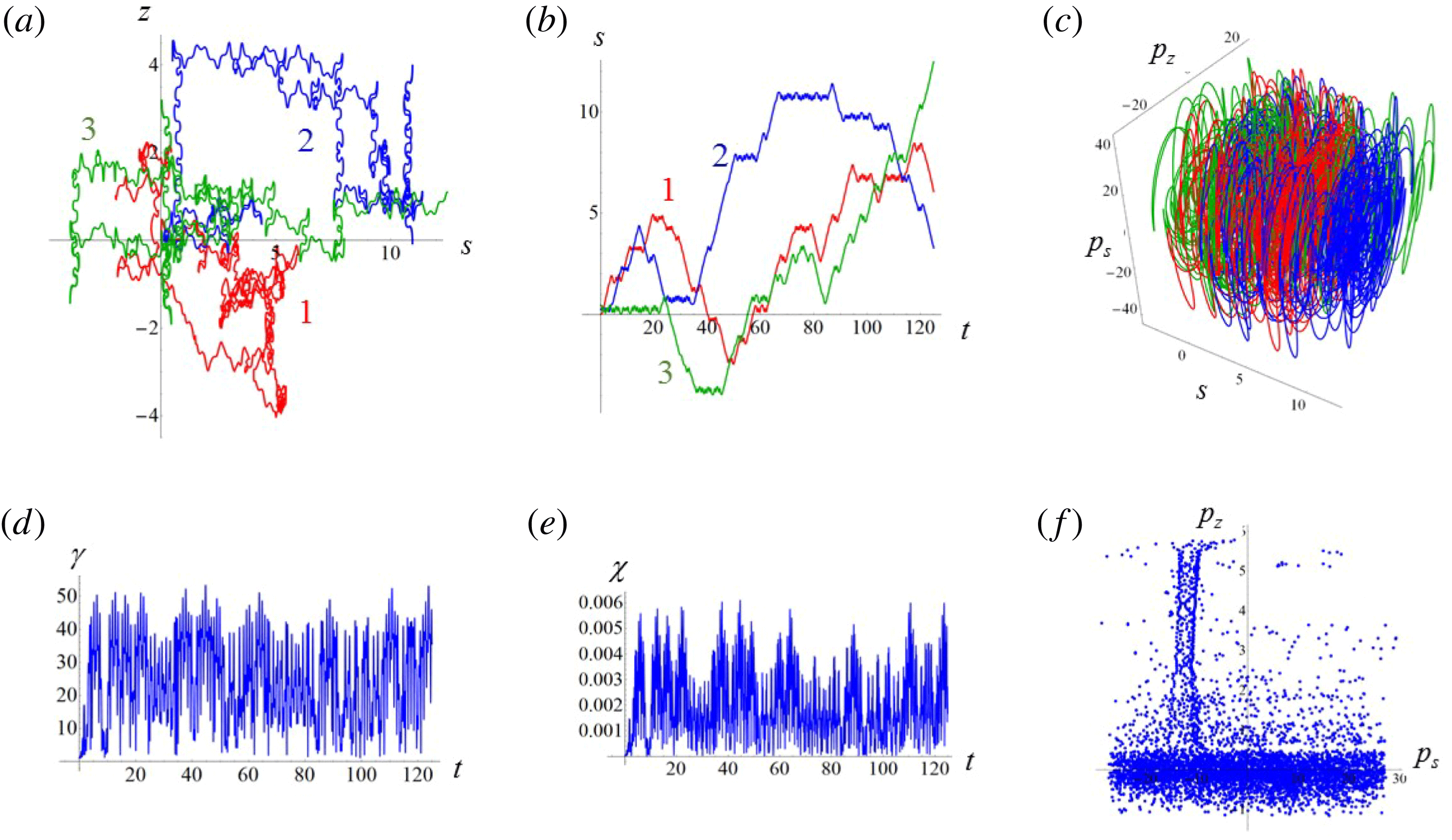
Electron trajectories in the case of the second type particular solution corresponding to the motion along the
 $x=y$
direction in the field of four colliding EM waves for
$x=y$
direction in the field of four colliding EM waves for
 $\unicode[STIX]{x1D700}_{rad}=1.2\times 10^{-8}$
,
$\unicode[STIX]{x1D700}_{rad}=1.2\times 10^{-8}$
,
 $a_{S}=4\times 10^{5}$
,
$a_{S}=4\times 10^{5}$
,
 $a_{0}=874$
,
$a_{0}=874$
,
 $\unicode[STIX]{x1D714}=1$
for initial conditions:
$\unicode[STIX]{x1D714}=1$
for initial conditions:
 $x(0)=0.01$
,
$x(0)=0.01$
,
 $z(0)=0$
,
$z(0)=0$
,
 $p_{x}(0)=0$
,
$p_{x}(0)=0$
,
 $p_{z}(0)=0$
(red,
$p_{z}(0)=0$
(red,
 $-1$
);
$-1$
);
 $x(0)=0.23$
,
$x(0)=0.23$
,
 $z(0)=0$
,
$z(0)=0$
,
 $p_{x}(0)=0$
,
$p_{x}(0)=0$
,
 $p_{z}(0)=0$
(blue,
$p_{z}(0)=0$
(blue,
 $-2$
);
$-2$
);
 $x(0)=0.45$
,
$x(0)=0.45$
,
 $z(0)=0$
,
$z(0)=0$
,
 $p_{x}(0)=0$
,
$p_{x}(0)=0$
,
 $p_{z}(0)=0$
(green,
$p_{z}(0)=0$
(green,
 $-3$
). (a) Trajectories in the
$-3$
). (a) Trajectories in the
 $(s,z)$
plane. (b) Dependences of the
$(s,z)$
plane. (b) Dependences of the
 $s$
coordinates on time. (c) Trajectories in the
$s$
coordinates on time. (c) Trajectories in the
 $(s,p_{s},p_{z})$
space. (d) Lorentz factor
$(s,p_{s},p_{z})$
space. (d) Lorentz factor
 $\unicode[STIX]{x1D6FE}$
versus time for
$\unicode[STIX]{x1D6FE}$
versus time for
 $x(0)=0.45$
. (e) Parameter
$x(0)=0.45$
. (e) Parameter
 $\unicode[STIX]{x1D712}_{e}$
versus time for
$\unicode[STIX]{x1D712}_{e}$
versus time for
 $x(0)=0.45$
. (f) The Poincaŕe sections: the particle positions in the phase plane
$x(0)=0.45$
. (f) The Poincaŕe sections: the particle positions in the phase plane
 $(p_{s},p_{z})$
at discrete times with the time step equal to the period of the driving force for
$(p_{s},p_{z})$
at discrete times with the time step equal to the period of the driving force for
 $x(0)=0.01$
.
$x(0)=0.01$
.
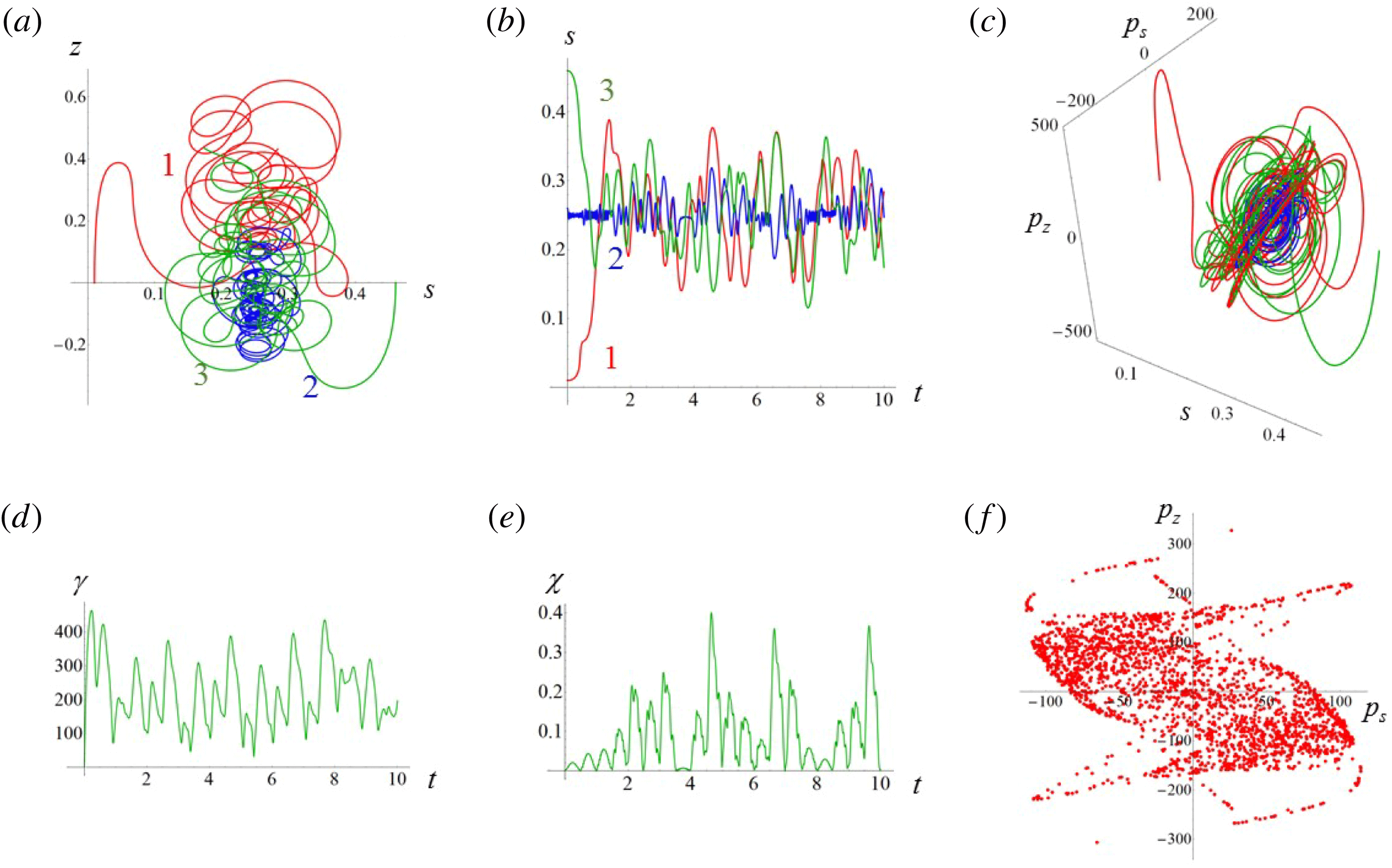
In figure 23 we present electron trajectories in the case corresponding to the motion along the
 $x=y$
direction in the field of four colliding EM waves for
$x=y$
direction in the field of four colliding EM waves for
 $\unicode[STIX]{x1D700}_{rad}=1.2\times 10^{-8}$
,
$\unicode[STIX]{x1D700}_{rad}=1.2\times 10^{-8}$
,
 $a_{S}=4\times 10^{5}$
,
$a_{S}=4\times 10^{5}$
,
 $a_{0}=44$
,
$a_{0}=44$
,
 $\unicode[STIX]{x1D714}=1$
for initial conditions:
$\unicode[STIX]{x1D714}=1$
for initial conditions:
 $x(0)=0.01$
,
$x(0)=0.01$
,
 $z(0)=0$
,
$z(0)=0$
,
 $p_{x}(0)=0$
,
$p_{x}(0)=0$
,
 $p_{z}(0)=0$
(red,
$p_{z}(0)=0$
(red,
 $-1$
);
$-1$
);
 $x(0)=0.23$
,
$x(0)=0.23$
,
 $z(0)=0$
,
$z(0)=0$
,
 $p_{x}(0)=0$
,
$p_{x}(0)=0$
,
 $p_{z}(0)=0$
(blue,
$p_{z}(0)=0$
(blue,
 $-2$
);
$-2$
);
 $x(0)=0.45$
,
$x(0)=0.45$
,
 $z(0)=0$
,
$z(0)=0$
,
 $p_{x}(0)=0$
,
$p_{x}(0)=0$
,
 $p_{z}(0)=0$
(green,
$p_{z}(0)=0$
(green,
 $-3$
). Figure 23(a) shows electron trajectories in the
$-3$
). Figure 23(a) shows electron trajectories in the
 $(s,z)$
plane, which demonstrate random walks with intermittent short scale-length oscillations and long range Lévy flights. The same behaviour is distinctly seen in figure 23(b) with three dependences of the
$(s,z)$
plane, which demonstrate random walks with intermittent short scale-length oscillations and long range Lévy flights. The same behaviour is distinctly seen in figure 23(b) with three dependences of the
 $s$
coordinates on time. Stochastic character of the particle motion is demonstrated in figure 23(b,f) by the behaviour of trajectories in the
$s$
coordinates on time. Stochastic character of the particle motion is demonstrated in figure 23(b,f) by the behaviour of trajectories in the
 $(s,p_{s},p_{z})$
space and by the particle positions in the phase plane
$(s,p_{s},p_{z})$
space and by the particle positions in the phase plane
 $(p_{s},p_{z})$
at discrete times with the time step equal to the period of the driving force, respectively. According to figure 23(d), where the particle Lorentz factor
$(p_{s},p_{z})$
at discrete times with the time step equal to the period of the driving force, respectively. According to figure 23(d), where the particle Lorentz factor
 $\unicode[STIX]{x1D6FE}$
is plotted versus time, the normalized electron energy is of the order of the dimensionless EM field amplitude, i.e.
$\unicode[STIX]{x1D6FE}$
is plotted versus time, the normalized electron energy is of the order of the dimensionless EM field amplitude, i.e.
 $\unicode[STIX]{x1D6FE}\approx a_{0}$
. From the dependence of the parameter
$\unicode[STIX]{x1D6FE}\approx a_{0}$
. From the dependence of the parameter
 $\unicode[STIX]{x1D712}$
on time in figure 23(e) it follows that, in this case, the QED effect of the recoil is not significant.
$\unicode[STIX]{x1D712}$
on time in figure 23(e) it follows that, in this case, the QED effect of the recoil is not significant.
The electron interaction with four colliding EM waves in the case of the second type particular solution corresponding to the motion along the
 $x=y$
direction is illustrated in figure 24 for
$x=y$
direction is illustrated in figure 24 for
 $\unicode[STIX]{x1D700}_{rad}=1.2\times 10^{-8}$
,
$\unicode[STIX]{x1D700}_{rad}=1.2\times 10^{-8}$
,
 $a_{S}=4\times 10^{5}$
,
$a_{S}=4\times 10^{5}$
,
 $a_{0}=874$
,
$a_{0}=874$
,
 $\unicode[STIX]{x1D714}=1$
for initial conditions:
$\unicode[STIX]{x1D714}=1$
for initial conditions:
 $x(0)=0.01$
,
$x(0)=0.01$
,
 $z(0)=0$
,
$z(0)=0$
,
 $p_{x}(0)=0$
,
$p_{x}(0)=0$
,
 $p_{z}(0)=0$
(red,
$p_{z}(0)=0$
(red,
 $-1$
);
$-1$
);
 $x(0)=0.23$
,
$x(0)=0.23$
,
 $z(0)=0$
,
$z(0)=0$
,
 $p_{x}(0)=0$
,
$p_{x}(0)=0$
,
 $p_{z}(0)=0$
(blue,
$p_{z}(0)=0$
(blue,
 $-2$
);
$-2$
);
 $x(0)=0.45$
,
$x(0)=0.45$
,
 $z(0)=0$
,
$z(0)=0$
,
 $p_{x}(0)=0$
,
$p_{x}(0)=0$
,
 $p_{z}(0)=0$
(green,
$p_{z}(0)=0$
(green,
 $-3$
). The particle independently of the initial conditions becomes trapped by a strange attractor performing stochastic motion. Panel figure 24(a) shows trajectories in the
$-3$
). The particle independently of the initial conditions becomes trapped by a strange attractor performing stochastic motion. Panel figure 24(a) shows trajectories in the
 $(s,z)$
plane. As we see the electrons become trapped in the region of the ponderomotive force minimum. From figure 25(b,c) with dependences of the
$(s,z)$
plane. As we see the electrons become trapped in the region of the ponderomotive force minimum. From figure 25(b,c) with dependences of the
 $s$
coordinates on time and with the trajectories in the
$s$
coordinates on time and with the trajectories in the
 $(s,p_{s},p_{z})$
space it follows that the trapped particle motion with all the three initial conditions is irregular. As we may see in figure 24(d), where the Lorentz factor
$(s,p_{s},p_{z})$
space it follows that the trapped particle motion with all the three initial conditions is irregular. As we may see in figure 24(d), where the Lorentz factor
 $\unicode[STIX]{x1D6FE}$
versus time for
$\unicode[STIX]{x1D6FE}$
versus time for
 $x(0)=0.23$
is presented, the normalized particle energy is of the order of the dimensionless EM wave amplitude. The QED parameter
$x(0)=0.23$
is presented, the normalized particle energy is of the order of the dimensionless EM wave amplitude. The QED parameter
 $\unicode[STIX]{x1D712}_{e}$
, whose dependence on time for
$\unicode[STIX]{x1D712}_{e}$
, whose dependence on time for
 $x(0)=0.23$
is shown in figure 24(e) is lower than unity, i.e. the QED effect of the recoil is weak. The Poincaŕe sections are shown in figure 24(e): the particle positions in the phase plane
$x(0)=0.23$
is shown in figure 24(e) is lower than unity, i.e. the QED effect of the recoil is weak. The Poincaŕe sections are shown in figure 24(e): the particle positions in the phase plane
 $(p_{s},p_{z})$
at discrete times with the time step equal to the period of the driving force for
$(p_{s},p_{z})$
at discrete times with the time step equal to the period of the driving force for
 $x(0)=0.01$
. As we see, the particle motion is stochastic.
$x(0)=0.01$
. As we see, the particle motion is stochastic.
Electron trajectories in the case of the second type particular solution corresponding to the motion along the
 $x=y$
direction in the field of four colliding EM waves for
$x=y$
direction in the field of four colliding EM waves for
 $\unicode[STIX]{x1D700}_{rad}=3\times 10^{-9}$
,
$\unicode[STIX]{x1D700}_{rad}=3\times 10^{-9}$
,
 $a_{S}=1.6\times 10^{6}$
,
$a_{S}=1.6\times 10^{6}$
,
 $a_{0}=3466$
,
$a_{0}=3466$
,
 $\unicode[STIX]{x1D714}=0.25$
for initial conditions:
$\unicode[STIX]{x1D714}=0.25$
for initial conditions:
 $x(0)=0.01$
,
$x(0)=0.01$
,
 $z(0)=0$
,
$z(0)=0$
,
 $p_{x}(0)=0$
,
$p_{x}(0)=0$
,
 $p_{z}(0)=0$
(red,
$p_{z}(0)=0$
(red,
 $-1$
);
$-1$
);
 $x(0)=0.23$
,
$x(0)=0.23$
,
 $z(0)=0$
,
$z(0)=0$
,
 $p_{x}(0)=0$
,
$p_{x}(0)=0$
,
 $p_{z}(0)=0$
(blue,
$p_{z}(0)=0$
(blue,
 $-2$
);
$-2$
);
 $x(0)=0.45$
,
$x(0)=0.45$
,
 $z(0)=0$
,
$z(0)=0$
,
 $p_{x}(0)=0$
,
$p_{x}(0)=0$
,
 $p_{z}(0)=0$
(green,
$p_{z}(0)=0$
(green,
 $-3$
). (a) Trajectories in the
$-3$
). (a) Trajectories in the
 $(s,z)$
plane. (b) Dependences of the
$(s,z)$
plane. (b) Dependences of the
 $s$
coordinates on time. (c) Trajectories in the
$s$
coordinates on time. (c) Trajectories in the
 $(s,p_{s},p_{z})$
space. The inset shows a close up of trajectories in the
$(s,p_{s},p_{z})$
space. The inset shows a close up of trajectories in the
 $(s,p_{s},p_{z})$
for
$(s,p_{s},p_{z})$
for
 $x(0)=0.23$
. (d) Lorentz factor
$x(0)=0.23$
. (d) Lorentz factor
 $\unicode[STIX]{x1D6FE}$
versus time for
$\unicode[STIX]{x1D6FE}$
versus time for
 $x(0)=0.23$
. (e) Parameter
$x(0)=0.23$
. (e) Parameter
 $\unicode[STIX]{x1D712}_{e}$
versus time for
$\unicode[STIX]{x1D712}_{e}$
versus time for
 $x(0)=0.23$
. (f) The Poincaŕe sections: the particle positions in the phase plane
$x(0)=0.23$
. (f) The Poincaŕe sections: the particle positions in the phase plane
 $(p_{s},p_{z})$
at discrete times with the time step equal to the period of the driving force for
$(p_{s},p_{z})$
at discrete times with the time step equal to the period of the driving force for
 $x(0)=0.23$
.
$x(0)=0.23$
.
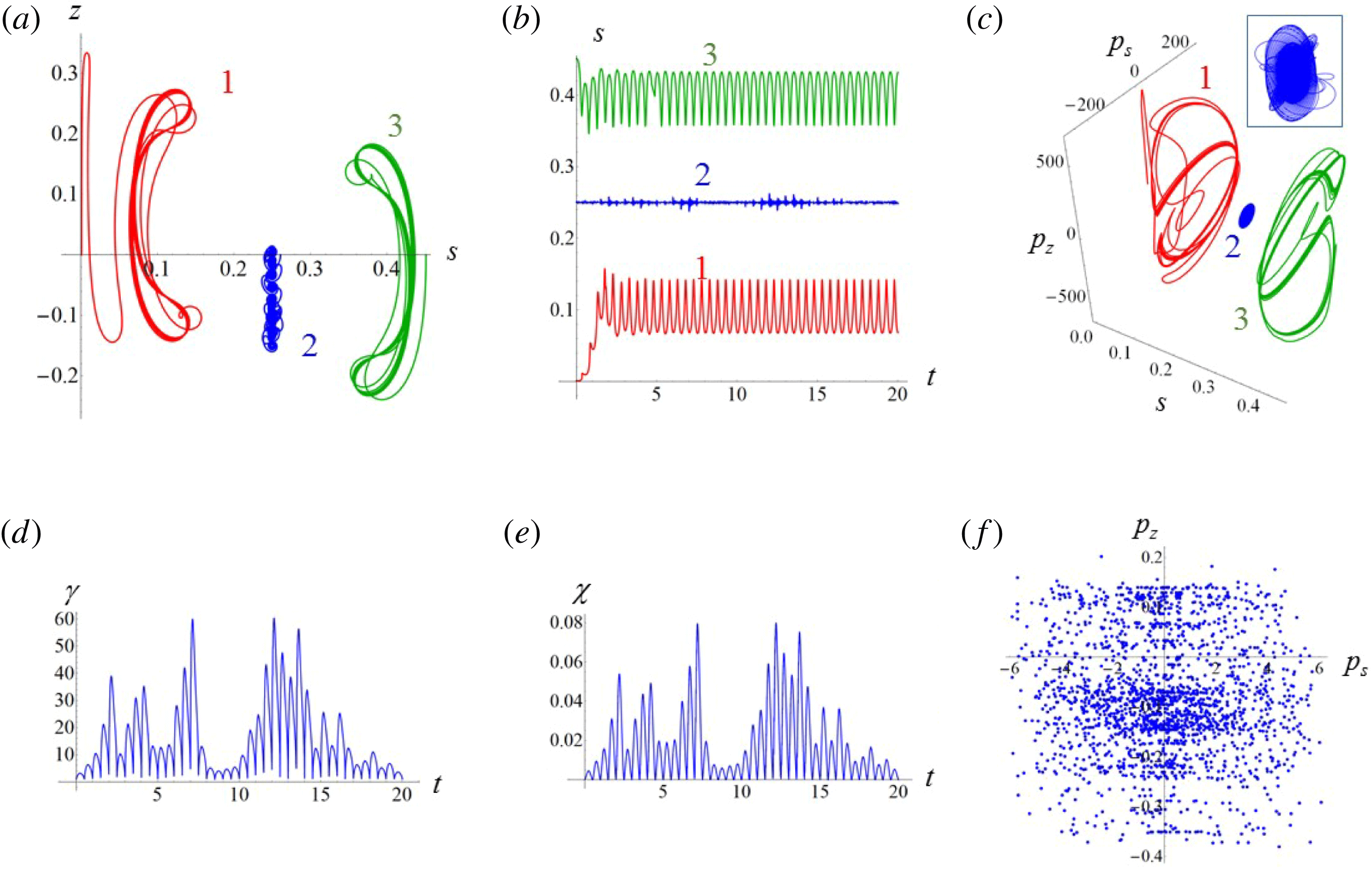
Electron interaction with four colliding EM waves in the case of the second type particular solution corresponding to the motion along the
 $x=y$
direction is illustrated in figure 25 for
$x=y$
direction is illustrated in figure 25 for
 $\unicode[STIX]{x1D700}_{rad}=3\times 10^{-9}$
,
$\unicode[STIX]{x1D700}_{rad}=3\times 10^{-9}$
,
 $a_{S}=1.6\times 10^{6}$
,
$a_{S}=1.6\times 10^{6}$
,
 $a_{0}=3466$
,
$a_{0}=3466$
,
 $\unicode[STIX]{x1D714}=0.25$
for initial conditions:
$\unicode[STIX]{x1D714}=0.25$
for initial conditions:
 $x(0)=0.01$
,
$x(0)=0.01$
,
 $z(0)=0$
,
$z(0)=0$
,
 $p_{x}(0)=0$
,
$p_{x}(0)=0$
,
 $p_{z}(0)=0$
(red,
$p_{z}(0)=0$
(red,
 $-1$
);
$-1$
);
 $x(0)=0.23$
,
$x(0)=0.23$
,
 $z(0)=0$
,
$z(0)=0$
,
 $p_{x}(0)=0$
,
$p_{x}(0)=0$
,
 $p_{z}(0)=0$
(blue,
$p_{z}(0)=0$
(blue,
 $-2$
);
$-2$
);
 $x(0)=0.45$
,
$x(0)=0.45$
,
 $z(0)=0$
,
$z(0)=0$
,
 $p_{x}(0)=0$
,
$p_{x}(0)=0$
,
 $p_{z}(0)=0$
(green,
$p_{z}(0)=0$
(green,
 $-3$
). In this case the EM wave frequency is lower than in the above discussed case and the EM wave amplitude is higher. As a result the particle is trapped performing either regular or stochastic motion. Panel figure 25(a) shows trajectories in the
$-3$
). In this case the EM wave frequency is lower than in the above discussed case and the EM wave amplitude is higher. As a result the particle is trapped performing either regular or stochastic motion. Panel figure 25(a) shows trajectories in the
 $(s,z)$
plane. As we see, depending on the initial conditions, the electron becomes trapped either in the region of the ponderomotive force maximum or in the region of its minimum. From figure 25(b,c) with dependences of the
$(s,z)$
plane. As we see, depending on the initial conditions, the electron becomes trapped either in the region of the ponderomotive force maximum or in the region of its minimum. From figure 25(b,c) with dependences of the
 $s$
coordinates on time and with the trajectories in the
$s$
coordinates on time and with the trajectories in the
 $(s,p_{s},p_{z})$
space it follows that the trapped particle motion with the initial conditions
$(s,p_{s},p_{z})$
space it follows that the trapped particle motion with the initial conditions
 $x(0)=0.01$
and
$x(0)=0.01$
and
 $x(0)=0.45$
along the limit circles is regular. As one can see in figure 25(d), where the Lorentz factor
$x(0)=0.45$
along the limit circles is regular. As one can see in figure 25(d), where the Lorentz factor
 $\unicode[STIX]{x1D6FE}$
versus time for
$\unicode[STIX]{x1D6FE}$
versus time for
 $x(0)=0.23$
is presented, the normalized particle energy is substantially lower than the dimensionless EM wave amplitude. The QED parameter
$x(0)=0.23$
is presented, the normalized particle energy is substantially lower than the dimensionless EM wave amplitude. The QED parameter
 $\unicode[STIX]{x1D712}_{e}$
, whose dependence on time for
$\unicode[STIX]{x1D712}_{e}$
, whose dependence on time for
 $x(0)=0.23$
is shown figure 25(e) is significantly lower than unity, i.e. the QED effect of the recoil is negligibly weak. The Poincaŕe sections are shown in figure 25(e), the particle positions in the phase plane
$x(0)=0.23$
is shown figure 25(e) is significantly lower than unity, i.e. the QED effect of the recoil is negligibly weak. The Poincaŕe sections are shown in figure 25(e), the particle positions in the phase plane
 $(p_{s},p_{z})$
at discrete times with the time step equal to the period of the driving force for
$(p_{s},p_{z})$
at discrete times with the time step equal to the period of the driving force for
 $x(0)=0.23$
. As we see, the particle motion along the trajectories of the attractor plotted in the inset in figure 25(c) with the close up of trajectories in the
$x(0)=0.23$
. As we see, the particle motion along the trajectories of the attractor plotted in the inset in figure 25(c) with the close up of trajectories in the
 $(s,p_{s},p_{z})$
for
$(s,p_{s},p_{z})$
for
 $x(0)=0.23$
is stochastic.
$x(0)=0.23$
is stochastic.
6.1.3 General case
The results of integration of the motion equations for the electron interacting with four s-polarized EM waves in the limit of relatively low radiation intensity are presented in figure 26. Figure 26(a) shows 11 electron trajectories in the
 $(x,y)$
plane for initial conditions as follows. The initial coordinates
$(x,y)$
plane for initial conditions as follows. The initial coordinates
 $x(0)$
and
$x(0)$
and
 $y(0)$
are chosen to be in the vicinity of the coordinate origin, and
$y(0)$
are chosen to be in the vicinity of the coordinate origin, and
 $z(0)=0$
,
$z(0)=0$
,
 $p_{x}(0)=0$
,
$p_{x}(0)=0$
,
 $p_{y}(0)=0$
,
$p_{y}(0)=0$
,
 $p_{z}(0)=0$
. In figure 26(b) we show a close up of the trajectories in the vicinity of the coordinate origin superimposed with the isocontours of the electromagnetic potential averaged over a half-period of the field oscillations. It is proportional to the ponderomotive potential in the high field amplitude limit,
$p_{z}(0)=0$
. In figure 26(b) we show a close up of the trajectories in the vicinity of the coordinate origin superimposed with the isocontours of the electromagnetic potential averaged over a half-period of the field oscillations. It is proportional to the ponderomotive potential in the high field amplitude limit,
 $a_{0}\gg 1$
. As we see, the typical trajectories are comprised of long range Lévy-flight-like excursions and of short range rambling motion, which changes the direction of the succeeding flight. The corresponding particle trajectory in the
$a_{0}\gg 1$
. As we see, the typical trajectories are comprised of long range Lévy-flight-like excursions and of short range rambling motion, which changes the direction of the succeeding flight. The corresponding particle trajectory in the
 $(p_{x},p_{y},p_{z})$
momentum space for
$(p_{x},p_{y},p_{z})$
momentum space for
 $x(0)=-0.125$
and
$x(0)=-0.125$
and
 $y(0)=0.125$
is presented figure 26(c). According to the dependence of the parameter
$y(0)=0.125$
is presented figure 26(c). According to the dependence of the parameter
 $\unicode[STIX]{x1D712}_{e}$
on time plotted in figure 26(d) the QED recoil effects are weak under the conditions of consideration. The Poincaŕe sections, the particle positions in the phase plane
$\unicode[STIX]{x1D712}_{e}$
on time plotted in figure 26(d) the QED recoil effects are weak under the conditions of consideration. The Poincaŕe sections, the particle positions in the phase plane
 $(p_{x},p_{y})$
at discrete times with the time step equal to the period of the driving force, in figure 26(e), show that the particle motion is stochastic.
$(p_{x},p_{y})$
at discrete times with the time step equal to the period of the driving force, in figure 26(e), show that the particle motion is stochastic.
(a) Eleven electron trajectories in the
 $(x,y)$
plane for initial conditions:
$(x,y)$
plane for initial conditions:
 $x(0)$
and
$x(0)$
and
 $y(0)$
are in the vicinity of the coordinate origin, and
$y(0)$
are in the vicinity of the coordinate origin, and
 $z(0)=0$
,
$z(0)=0$
,
 $p_{x}(0)=0$
,
$p_{x}(0)=0$
,
 $p_{y}(0)=0$
,
$p_{y}(0)=0$
,
 $p_{z}(0)=0$
. (b) Close up of the trajectories in the region
$p_{z}(0)=0$
. (b) Close up of the trajectories in the region
 $(-7.5<x<7.5;-7.5<y<7.5)$
. (c) Trajectory in the
$(-7.5<x<7.5;-7.5<y<7.5)$
. (c) Trajectory in the
 $(p_{x},p_{y},p_{z})$
space. (d) Parameter
$(p_{x},p_{y},p_{z})$
space. (d) Parameter
 $\unicode[STIX]{x1D712}_{e}$
versus time. (e) The Poincaŕe sections: the particle positions in the phase plane
$\unicode[STIX]{x1D712}_{e}$
versus time. (e) The Poincaŕe sections: the particle positions in the phase plane
 $(p_{x},p_{y})$
at discrete times with the time step equal to the period of the driving force. The electromagnetic field amplitude is
$(p_{x},p_{y})$
at discrete times with the time step equal to the period of the driving force. The electromagnetic field amplitude is
 $a_{0}=218$
, the dissipation parameter is
$a_{0}=218$
, the dissipation parameter is
 $\unicode[STIX]{x1D700}_{rad}=1.2\times 10^{-8}$
, the normalized critical QED field is
$\unicode[STIX]{x1D700}_{rad}=1.2\times 10^{-8}$
, the normalized critical QED field is
 $a_{S}=4\times 10^{5}$
and the EM field frequency equals
$a_{S}=4\times 10^{5}$
and the EM field frequency equals
 $\unicode[STIX]{x1D714}_{0}=1$
.
$\unicode[STIX]{x1D714}_{0}=1$
.
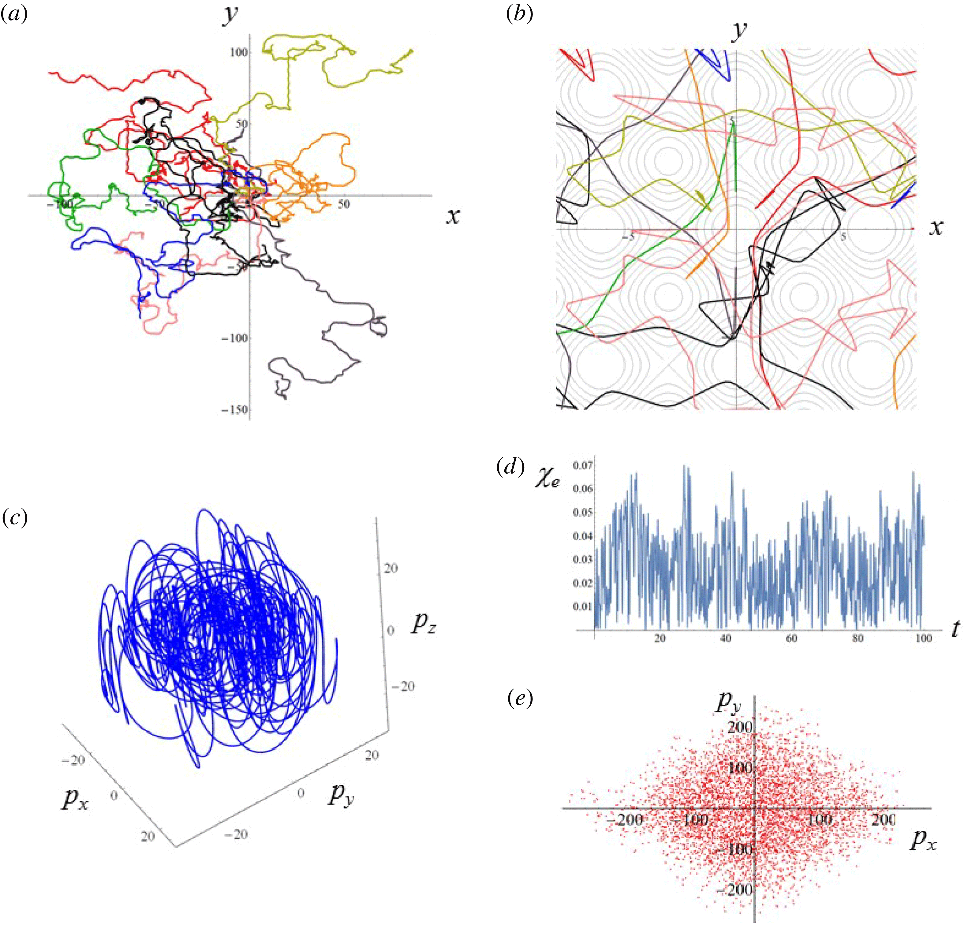
(a) Eleven electron trajectories in the
 $(x,y)$
plane for initial conditions:
$(x,y)$
plane for initial conditions:
 $x(0)$
and
$x(0)$
and
 $y(0)$
are in the vicinity of the coordinate origin, and
$y(0)$
are in the vicinity of the coordinate origin, and
 $z(0)=0$
,
$z(0)=0$
,
 $p_{x}(0)=0$
,
$p_{x}(0)=0$
,
 $p_{y}(0)=0$
,
$p_{y}(0)=0$
,
 $p_{z}(0)=0$
. (b) Close up of the trajectories in the region
$p_{z}(0)=0$
. (b) Close up of the trajectories in the region
 $(-10<x<10;-20<y<0)$
superimposed with the isocontours if the electromagnetic potential averaged over a half-period of the field oscillations. (c) Trajectory in the
$(-10<x<10;-20<y<0)$
superimposed with the isocontours if the electromagnetic potential averaged over a half-period of the field oscillations. (c) Trajectory in the
 $(p_{x},p_{y},p_{z})$
space. (d) Trajectory in the
$(p_{x},p_{y},p_{z})$
space. (d) Trajectory in the
 $(x,y,z)$
space. The electromagnetic field amplitude is
$(x,y,z)$
space. The electromagnetic field amplitude is
 $a_{0}=2823$
, the dissipation parameter is
$a_{0}=2823$
, the dissipation parameter is
 $\unicode[STIX]{x1D700}_{rad}=1.2\times 10^{-9}$
, the normalized critical QED field is
$\unicode[STIX]{x1D700}_{rad}=1.2\times 10^{-9}$
, the normalized critical QED field is
 $a_{S}=4\times 10^{6}$
and the EM field frequency equals
$a_{S}=4\times 10^{6}$
and the EM field frequency equals
 $\unicode[STIX]{x1D714}_{0}=0.1$
.
$\unicode[STIX]{x1D714}_{0}=0.1$
.
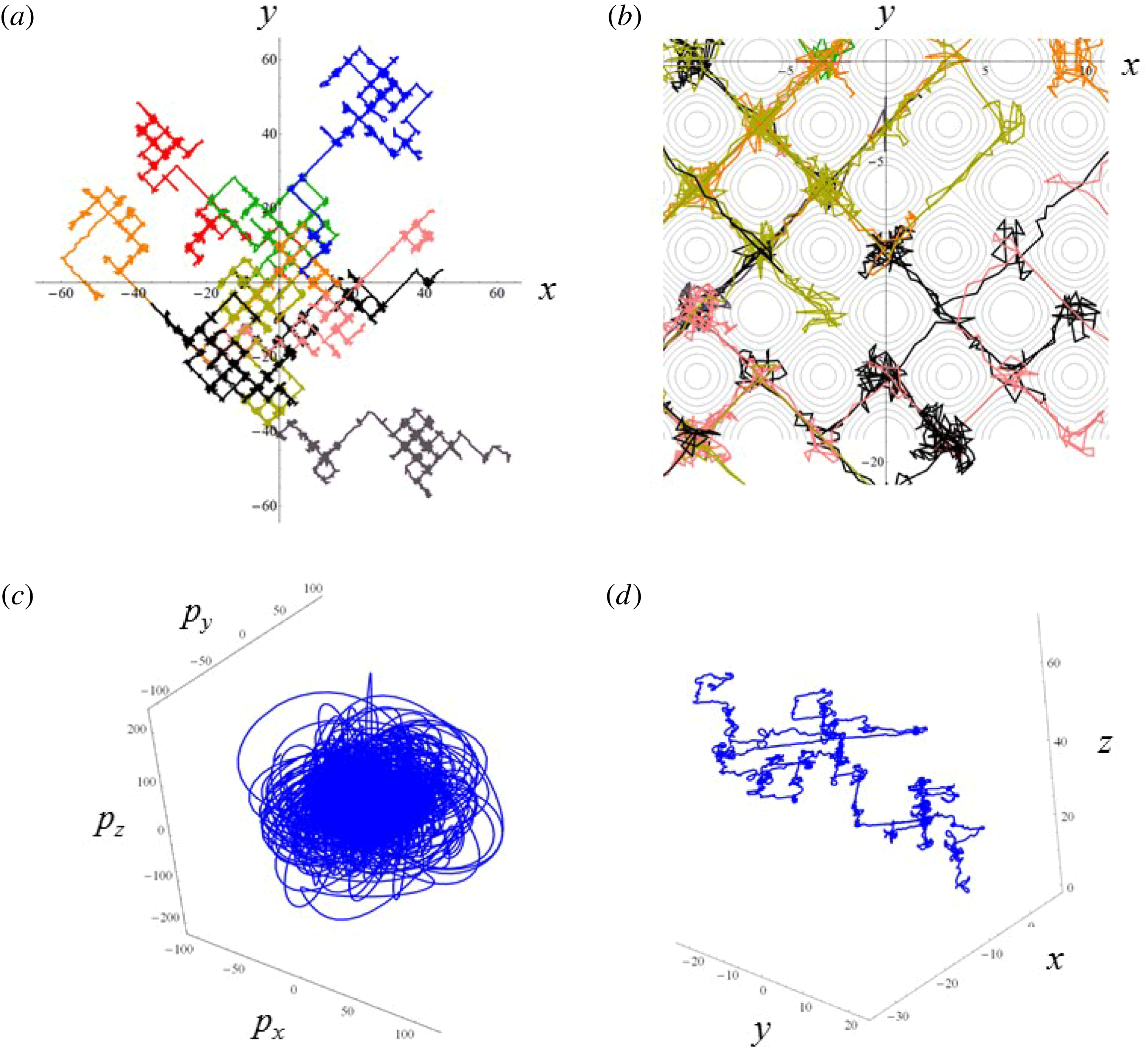
Figure 27 illustrates the particle dynamics in the EM field formed by four s-polarized EM waves for the radiation intensity higher than that intensity which corresponds to the interaction regime shown in figure 26. Here the electromagnetic field amplitude is
 $a_{0}=2823$
, the dissipation parameter is
$a_{0}=2823$
, the dissipation parameter is
 $\unicode[STIX]{x1D700}_{rad}=1.2\times 10^{-9}$
, the normalized critical QED field is
$\unicode[STIX]{x1D700}_{rad}=1.2\times 10^{-9}$
, the normalized critical QED field is
 $a_{S}=4\times 10^{6}$
and the EM field frequency equals
$a_{S}=4\times 10^{6}$
and the EM field frequency equals
 $\unicode[STIX]{x1D714}_{0}=0.1$
. From figure 27(a,b) it follows that the typical trajectories form a pretty regular pattern in the
$\unicode[STIX]{x1D714}_{0}=0.1$
. From figure 27(a,b) it follows that the typical trajectories form a pretty regular pattern in the
 $(x,y)$
plane. They are comprised of long range Lévy-flight-like excursions and of short range rambling motion, which changes the direction of the succeeding flight. The combination of the long range excursions and short range rambling is also seen in the behaviour of the electron trajectory in the
$(x,y)$
plane. They are comprised of long range Lévy-flight-like excursions and of short range rambling motion, which changes the direction of the succeeding flight. The combination of the long range excursions and short range rambling is also seen in the behaviour of the electron trajectory in the
 $(x,y,z)$
space presented in figure 27(d). The corresponding particle trajectory in the
$(x,y,z)$
space presented in figure 27(d). The corresponding particle trajectory in the
 $(p_{x},p_{y},p_{z})$
momentum space for
$(p_{x},p_{y},p_{z})$
momentum space for
 $x(0)=-0.125$
and
$x(0)=-0.125$
and
 $y(0)=0.125$
is presented in figure 27(c). What is remarkable is that during the Lévy like flights the electron moves almost along the electric node region, i.e. performing the motion described by the second type particular solution discussed above (see figure 24). The particle normalized energy changes from 200 to approximately 1200. The value of the QED dimensionless parameter
$y(0)=0.125$
is presented in figure 27(c). What is remarkable is that during the Lévy like flights the electron moves almost along the electric node region, i.e. performing the motion described by the second type particular solution discussed above (see figure 24). The particle normalized energy changes from 200 to approximately 1200. The value of the QED dimensionless parameter
 $\unicode[STIX]{x1D712}_{e}$
(not shown here) is less than unity. The Poincaŕe sections (also not shown here) are similar to those sections which are presented in figure 26(e) indicating stochasticity in the electron dynamics.
$\unicode[STIX]{x1D712}_{e}$
(not shown here) is less than unity. The Poincaŕe sections (also not shown here) are similar to those sections which are presented in figure 26(e) indicating stochasticity in the electron dynamics.
Further increasing the EM field intensity and/or decreasing the field frequency lead to an intriguing change in the trajectory pattern (see figure 28, where an ensemble of the electron trajectories in the
 $(x,y)$
plane is presented). The results presented in figures 28 and 29 have been obtained for the electromagnetic field amplitude of
$(x,y)$
plane is presented). The results presented in figures 28 and 29 have been obtained for the electromagnetic field amplitude of
 $a_{0}=11\,856$
, for the dissipation parameter of
$a_{0}=11\,856$
, for the dissipation parameter of
 $\unicode[STIX]{x1D700}_{rad}=6\times 10^{-10}$
, for the normalized critical QED field of
$\unicode[STIX]{x1D700}_{rad}=6\times 10^{-10}$
, for the normalized critical QED field of
 $a_{S}=8\times 10^{6}$
and for the EM field frequency equal to
$a_{S}=8\times 10^{6}$
and for the EM field frequency equal to
 $\unicode[STIX]{x1D714}_{0}=0.05$
. The trajectory topology can be subdivided into two classes depending on the particle initial conditions. If the particle is initially close to the bottom of the ponderomotive potential, i.e. close to the lines
$\unicode[STIX]{x1D714}_{0}=0.05$
. The trajectory topology can be subdivided into two classes depending on the particle initial conditions. If the particle is initially close to the bottom of the ponderomotive potential, i.e. close to the lines
 $x=\pm y=\unicode[STIX]{x03C0}n$
,
$x=\pm y=\unicode[STIX]{x03C0}n$
,
 $n=\ldots ,-2,-1,0,1,2,\ldots$
in the
$n=\ldots ,-2,-1,0,1,2,\ldots$
in the
 $(x,y)$
plane, it remains there. The particle trajectory, in this case, is similar to those shown in figure 27(a,b). The second class trajectories are realized for the initial particle positions in the vicinity of the ponderomotive potential maximum, where the magnetic field of the colliding EM waves vanishes. The second class trajectories are trapped within one of the sectors,
$(x,y)$
plane, it remains there. The particle trajectory, in this case, is similar to those shown in figure 27(a,b). The second class trajectories are realized for the initial particle positions in the vicinity of the ponderomotive potential maximum, where the magnetic field of the colliding EM waves vanishes. The second class trajectories are trapped within one of the sectors,
 $0<\unicode[STIX]{x1D703}<\unicode[STIX]{x03C0}/4$
,
$0<\unicode[STIX]{x1D703}<\unicode[STIX]{x03C0}/4$
,
 $\unicode[STIX]{x03C0}/4<\unicode[STIX]{x1D703}<\unicode[STIX]{x03C0}/2$
, etc. Oscillating along the radial direction they drift relatively slowly towards the lines either
$\unicode[STIX]{x03C0}/4<\unicode[STIX]{x1D703}<\unicode[STIX]{x03C0}/2$
, etc. Oscillating along the radial direction they drift relatively slowly towards the lines either
 $x=0$
or
$x=0$
or
 $y=0$
. In both the cases of the first and second topology classes the particles move also along the
$y=0$
. In both the cases of the first and second topology classes the particles move also along the
 $z$
axis as seen from the results presented in figure 29. The first class particle dynamics is stochastic: the trajectory in the
$z$
axis as seen from the results presented in figure 29. The first class particle dynamics is stochastic: the trajectory in the
 $(p_{x},p_{y},p_{z})$
space plotted in figure 29(d) corresponds to a strange attractor while figure 29(b) shows that the second class dynamics is regular.
$(p_{x},p_{y},p_{z})$
space plotted in figure 29(d) corresponds to a strange attractor while figure 29(b) shows that the second class dynamics is regular.
Ensemble of the electron trajectories in the
 $(x,y)$
plane. The particles with the initial coordinates in the region close to the
$(x,y)$
plane. The particles with the initial coordinates in the region close to the
 $B=0$
point are trapped inside the sectors, where their trajectories asymptotically approach the lines
$B=0$
point are trapped inside the sectors, where their trajectories asymptotically approach the lines
 $x=0$
or
$x=0$
or
 $y=0$
. For the initial coordinates close to the bottoms of the ponderomotive potential valleys,
$y=0$
. For the initial coordinates close to the bottoms of the ponderomotive potential valleys,
 $x=\pm y=\unicode[STIX]{x03C0}n$
,
$x=\pm y=\unicode[STIX]{x03C0}n$
,
 $n=\ldots ,-2,-1,0,1,2,\ldots$
the particles move along the trajectories which are similar to those shown in figure 27(a,b). The EM field amplitude is
$n=\ldots ,-2,-1,0,1,2,\ldots$
the particles move along the trajectories which are similar to those shown in figure 27(a,b). The EM field amplitude is
 $a_{0}=11\,856$
, the dissipation parameter is
$a_{0}=11\,856$
, the dissipation parameter is
 $\unicode[STIX]{x1D700}_{rad}=6\times 10^{-10}$
, the normalized critical QED field is
$\unicode[STIX]{x1D700}_{rad}=6\times 10^{-10}$
, the normalized critical QED field is
 $a_{S}=8\times 10^{6}$
and the EM field frequency equals
$a_{S}=8\times 10^{6}$
and the EM field frequency equals
 $\unicode[STIX]{x1D714}_{0}=0.05$
.
$\unicode[STIX]{x1D714}_{0}=0.05$
.
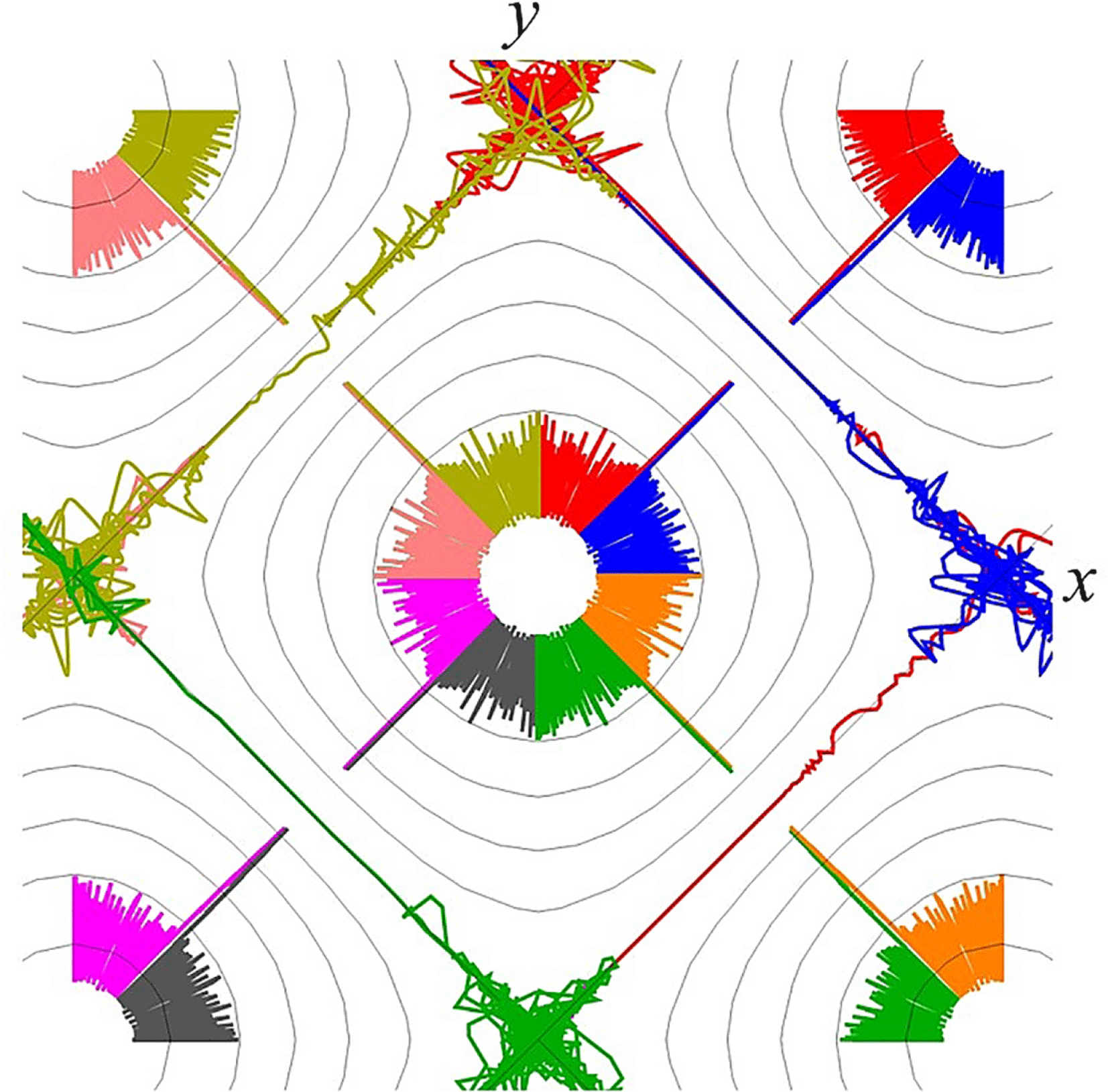
(a) Electron trajectory in the
 $(x,y,z)$
space and (b) trajectory in the
$(x,y,z)$
space and (b) trajectory in the
 $(p_{x},p_{y},p_{z})$
space for the second class topology. (c) Electron trajectory in the
$(p_{x},p_{y},p_{z})$
space for the second class topology. (c) Electron trajectory in the
 $(x,y,z)$
space and (d) trajectory in the
$(x,y,z)$
space and (d) trajectory in the
 $(p_{x},p_{y},p_{z})$
space for the first class topology. The electromagnetic field parameters are the same as in figure 28.
$(p_{x},p_{y},p_{z})$
space for the first class topology. The electromagnetic field parameters are the same as in figure 28.

6.2 Electron interaction with four p-polarized EM waves
In the case of four p-polarized colliding laser pulses the EM configuration is described by (6.1)–(6.3). As in the s-polarization case, in the limit of relatively low EM wave intensity the electron performs the random walk motion comprised of short scale-length oscillations interleaved by long scale excursions. An example of such trajectories is shown in figure 30(a) for the EM field amplitude
 $a_{0}=1.6\times 10^{3}$
, the dissipation parameter equal to
$a_{0}=1.6\times 10^{3}$
, the dissipation parameter equal to
 $\unicode[STIX]{x1D700}_{rad}=1.2\times 10^{-8}$
and the normalized critical QED field of
$\unicode[STIX]{x1D700}_{rad}=1.2\times 10^{-8}$
and the normalized critical QED field of
 $a_{S}=4.12\times 10^{5}$
. The curve marked by red colour and the number ‘1’ corresponds to the initial coordinates
$a_{S}=4.12\times 10^{5}$
. The curve marked by red colour and the number ‘1’ corresponds to the initial coordinates
 $x(0)=0.001$
and
$x(0)=0.001$
and
 $y(0)=0.01$
. Figure 30(b) presents a close up of trajectory (1) the
$y(0)=0.01$
. Figure 30(b) presents a close up of trajectory (1) the
 $(x,y)$
plane overlaid with the isocontours of the EM field ponderomotive potential. Electron oscillations in the
$(x,y)$
plane overlaid with the isocontours of the EM field ponderomotive potential. Electron oscillations in the
 $(p_{x},p_{y})$
plane (figure 30
c) and dependence of the
$(p_{x},p_{y})$
plane (figure 30
c) and dependence of the
 $y$
coordinate on time plotted in figure 30(d) demonstrate that the particle motion is irregular. The stochastic character of the particle dynamics is also distinctly seen in the Poincaŕe sections in the plane
$y$
coordinate on time plotted in figure 30(d) demonstrate that the particle motion is irregular. The stochastic character of the particle dynamics is also distinctly seen in the Poincaŕe sections in the plane
 $(p_{x},p_{y})$
, which is presented in figure 30(d).
$(p_{x},p_{y})$
, which is presented in figure 30(d).
Electron interaction with 4 colliding p-polarized EM waves in the low intensity limit for the electromagnetic field amplitude equal to
 $a_{0}=1.6\times 10^{3}$
, the dissipation parameter equal to
$a_{0}=1.6\times 10^{3}$
, the dissipation parameter equal to
 $\unicode[STIX]{x1D700}_{rad}=1.2\times 10^{-8}$
and the normalized critical QED field of
$\unicode[STIX]{x1D700}_{rad}=1.2\times 10^{-8}$
and the normalized critical QED field of
 $a_{S}=4.12\times 10^{5}$
. (a) Ensemble of electron trajectories in the
$a_{S}=4.12\times 10^{5}$
. (a) Ensemble of electron trajectories in the
 $(x,\,y)$
plane. Red colour (1) curve corresponds to
$(x,\,y)$
plane. Red colour (1) curve corresponds to
 $x(0)=0.001$
and
$x(0)=0.001$
and
 $y(0)=0.01$
. (b) Close up of trajectory (1) the
$y(0)=0.01$
. (b) Close up of trajectory (1) the
 $(x,y)$
plane overlaid with the isocontours of the EM field ponderomotive potential. (c) Electron trajectory in the
$(x,y)$
plane overlaid with the isocontours of the EM field ponderomotive potential. (c) Electron trajectory in the
 $(p_{x},p_{y})$
plane. (d) Coordinate
$(p_{x},p_{y})$
plane. (d) Coordinate
 $y$
versus time
$y$
versus time
 $t$
. (e) The Poincaŕe sections: the particle positions in the phase plane
$t$
. (e) The Poincaŕe sections: the particle positions in the phase plane
 $(p_{x},p_{y})$
at discrete times with the time step equal to the period of the driving force.
$(p_{x},p_{y})$
at discrete times with the time step equal to the period of the driving force.
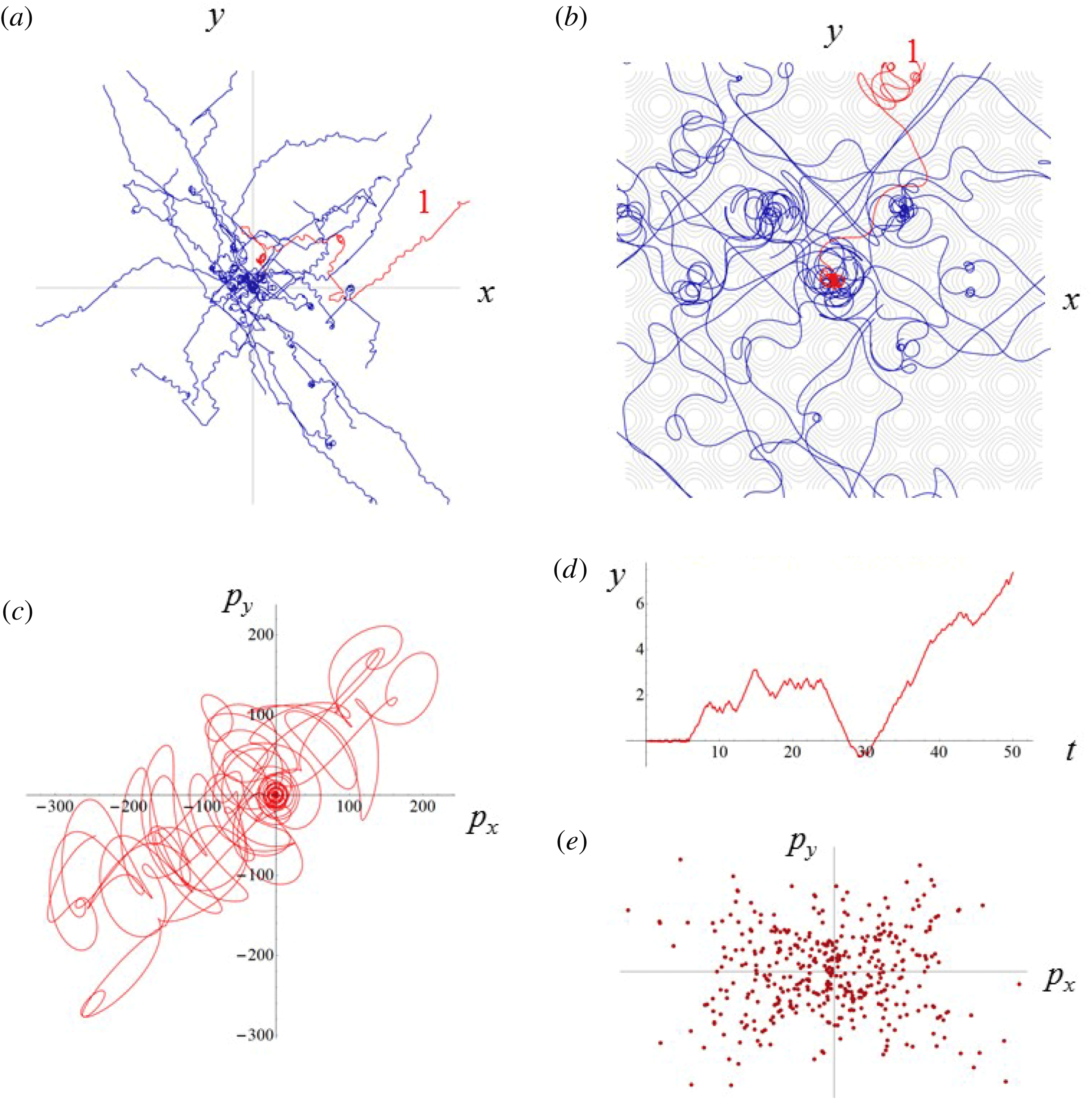
For ten times higher EM field amplitude, when
 $a_{0}=1.6\times 10^{4}$
, the particle motion becomes regular as seen in figure 31. In the
$a_{0}=1.6\times 10^{4}$
, the particle motion becomes regular as seen in figure 31. In the
 $(x,y)$
plane the electron performs long range Lévy-like flights along the lines
$(x,y)$
plane the electron performs long range Lévy-like flights along the lines
 $x=\pm y+\pm \unicode[STIX]{x03C0}n$
, which end up in the localized attractors, where the particle oscillates pretty regularly (see figure 31
a,b). This electron behaviour is well seen in figure 31(c–e) presenting the electron trajectory in the
$x=\pm y+\pm \unicode[STIX]{x03C0}n$
, which end up in the localized attractors, where the particle oscillates pretty regularly (see figure 31
a,b). This electron behaviour is well seen in figure 31(c–e) presenting the electron trajectory in the
 $(p_{x},p_{y})$
plane, the time dependence of the
$(p_{x},p_{y})$
plane, the time dependence of the
 $y$
coordinate and the Poincaŕe mapping in the momentum plane
$y$
coordinate and the Poincaŕe mapping in the momentum plane
 $(p_{x},p_{y})$
, respectively. Broadening of the trajectories in the Poincaŕe mapping figure 31(e) also indicates stochastic properties present in the particle motion.
$(p_{x},p_{y})$
, respectively. Broadening of the trajectories in the Poincaŕe mapping figure 31(e) also indicates stochastic properties present in the particle motion.
The same as in figure 30 for
 $a_{0}=1.6\times 10^{4}$
.
$a_{0}=1.6\times 10^{4}$
.
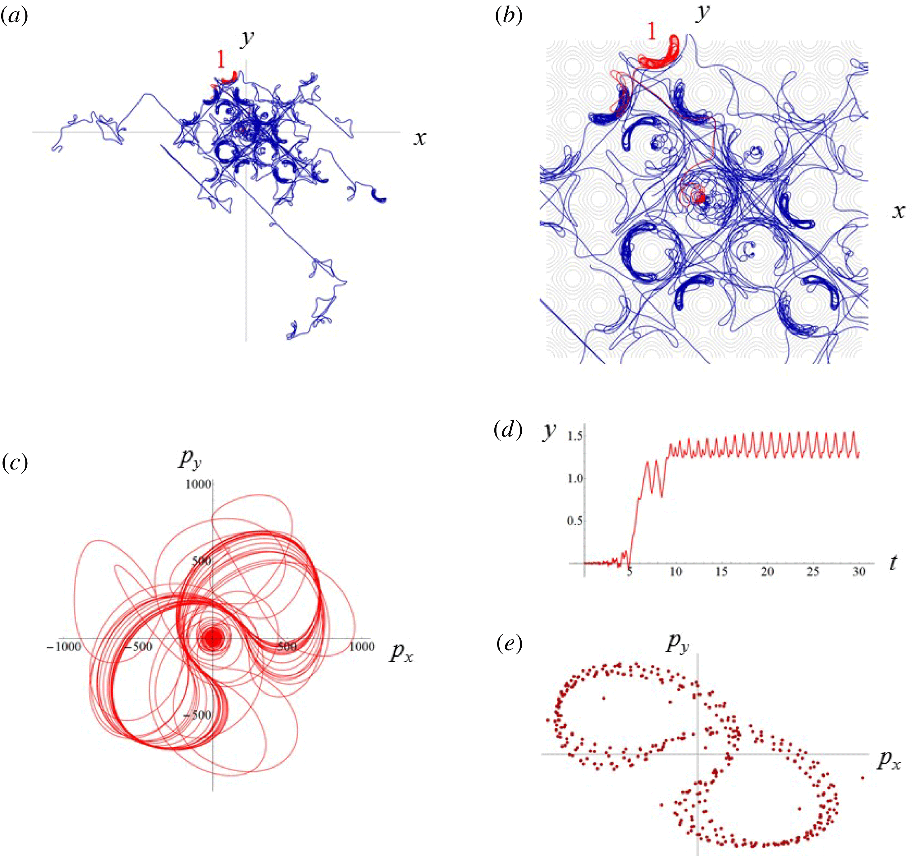
A further ten times increase of the EM field amplitude,
 $a_{0}=1.6\times 10^{5}$
, results in the particle trapping within narrow stripes localized at the bottoms of the ponderomotive potential (figure 32
a,b). A combination of regular and stochastic aspects of the particle dynamics in this case too is seen from the behaviour of the electron trajectory in the
$a_{0}=1.6\times 10^{5}$
, results in the particle trapping within narrow stripes localized at the bottoms of the ponderomotive potential (figure 32
a,b). A combination of regular and stochastic aspects of the particle dynamics in this case too is seen from the behaviour of the electron trajectory in the
 $(p_{x},p_{y})$
plane (figure 32
c), from the time dependence of the
$(p_{x},p_{y})$
plane (figure 32
c), from the time dependence of the
 $y$
coordinate (figure 32
d) and from the broadening of the trajectories in the Poincaŕe mapping (figure 32
d).
$y$
coordinate (figure 32
d) and from the broadening of the trajectories in the Poincaŕe mapping (figure 32
d).
The same as in figure 30 for
 $a_{0}=1.6\times 10^{5}$
.
$a_{0}=1.6\times 10^{5}$
.
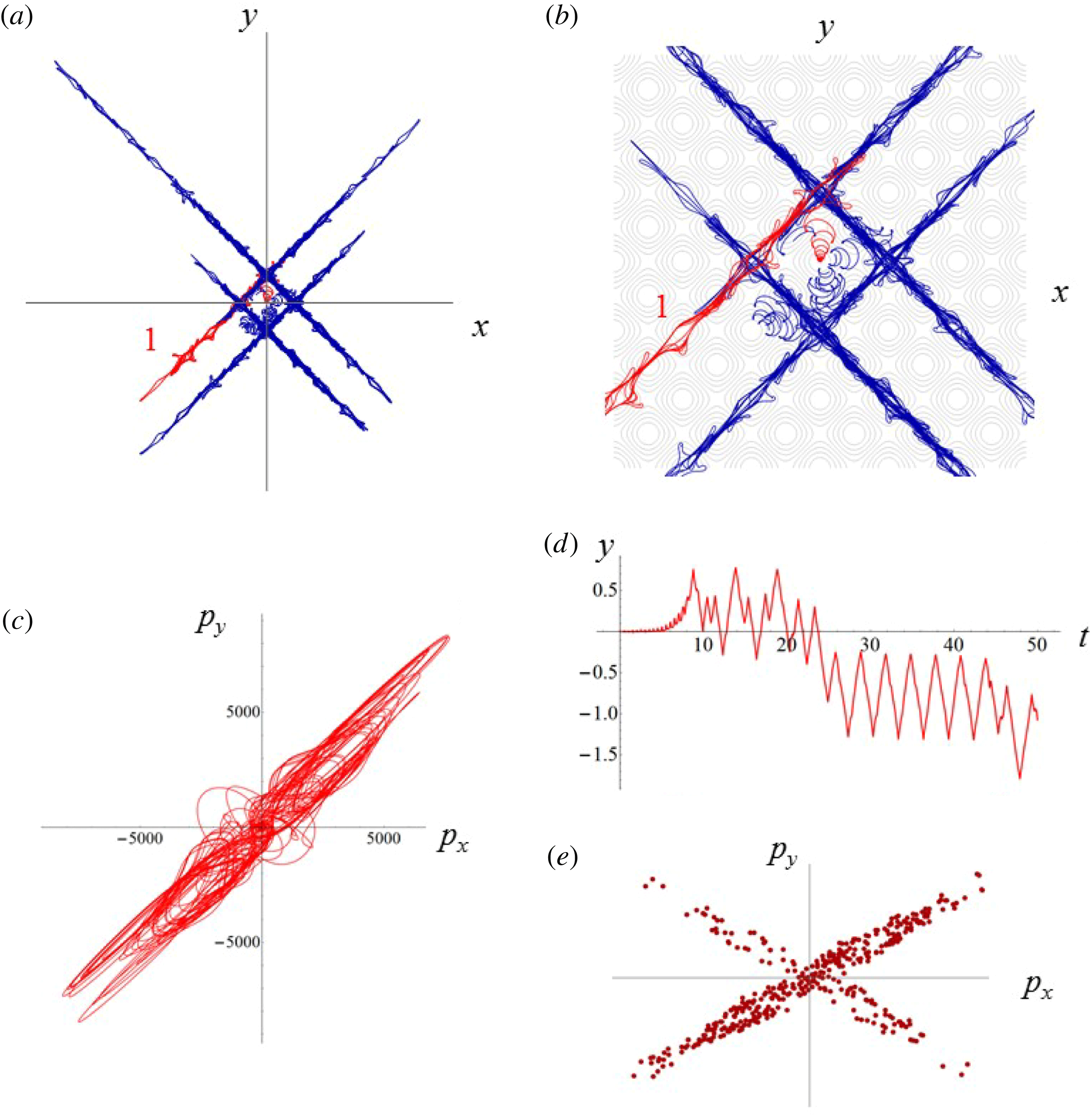
7 Conclusions
As is well known, the multiple colliding laser pulse concept (Bulanov et al. Reference Bulanov, Mur, Narozhny, Nees and Popov2010b ) is beneficial for achieving an extremely high amplitude of coherent electromagnetic field (see also Bulanov et al. Reference Bulanov, Esirkepov, Koga, Thomas and Bulanov2010a ; Gonoskov et al. Reference Gonoskov, Aiello, Heugel and Leuchs2012, Reference Gonoskov, Gonoskov, Harvey, Ilderton, Kim, Marklund, Mourou and Sergeev2013; Gelfer et al. Reference Gelfer, Mironov, Fedotov, Bashmakov, Nerush, Kostyukov and Narozhny2015). The complexity of the topology of the time-dependent EM field of colliding laser pulses results in the high complexity of the trajectories of charged particles interacting with these fields. In the high field limit, when the radiation friction effects become significant, the charged particle behaviour demonstrates remarkable features corresponding to random walk trajectories, Lévy flights, limit circles, attractors and regular patterns.
In the limit of the relatively weak laser intensity, the electron motion can be described as a random walk figure 5 with the particle over-leaping from one field period to another. The over-leaping correspond to the Lévy flights. In contrast to the standard theory of Lévy flights, which can be found in Lévy (Reference Lévy1954), Metzler & Klafter (Reference Metzler and Klafter2000), Zaslavsky (Reference Zaslavsky2002), Metzler et al. (Reference Metzler, Chechkin, Gonchar and Klafter2007), in the 3 and 4 colliding wave cases considered in the present paper, the Lévy-like flights occur along the directions determined by the landscape of the ponderomotive potential determined in its turn by the geometry of the EM field of the colliding waves. Typically the particle performs short space scale (high frequency) oscillations intermittent with the long range leaps. This oscillation frequency appears to be significantly higher than the frequency of the driver EM wave due to the nonlinearity of the radiation friction force (see also discussion in Esirkepov et al. Reference Esirkepov, Bulanov, Koga, Kando, Kondo, Rosanov, Korn and Bulanov2015; Jirka et al. Reference Jirka, Klimo, Bulanov, Esirkepov, Gelfer, Bulanov, Weber and Korn2016). The length of the long range flight can be found from consideration of the charged particle momentum losses due to radiation friction as in Bulanov et al. (Reference Bulanov, Esirkepov, Hayashi, Kando, Kiriyama, Koga, Kondo, Kotaki, Pirozhkov and Bulanov2011a ).
Under certain conditions (in the high intensity and/or low frequency limit) the nonlinear dissipation mechanism stabilizes the particle motion causing the particle trapping within a narrow region located near the electric field maximum. In high intensity limit the particle can be trapped in the vicinity of the EM field ponderomotive potential performing regular motion there. The particle trajectory makes regular patterns shown in figures 17 and 28.
We have analysed the underlying physical mechanism of the radiating charge particle trapping in the regions of the electric field maximum. As elucidated within the framework of the simple model formulated in the present paper the particle trapping is explained by the friction drag originating from the nonlinear dependence of the radiation friction on the EM field.
The attractor trajectory patterns in figures 17, 19 and 27 are made by an ensemble of electrons. The single electron trajectory shown in figure 18 demonstrates that having been moving for a long enough time it could cover the whole attractor. In view of this, there are two questions. The first one being is there an analogy of the ergodic hypothesis saying that over long periods of time, the time spent in some region of the attractor is proportional to the attractor measure? The second one being is there an analogy of the Poincaré recurrence theorem (Arnol’d Reference Arnol’d1989) saying that the particle, after a sufficiently long but finite time, returns to a point very close to the initial point? A similar question occurs in the case of the particle random walk on whether the results of the well-known random walk theory (see Kac Reference Kac1961) can be used in our case. Since finding the answers to these questions requires additional thorough consideration, we leave this to the forthcoming publications.
The structures seen in the electron density distribution obtained in the computer simulations of four electromagnetic pulse interaction with plasma targets (Vranic et al. Reference Vranic, Grismayer, Fonseca and Silva2017; Gong et al. Reference Gong, Hu, Shou, Qiao, Chen, He, Bulanov, Esirkepov, Bulanov and Yan2017) are similar to the structures presented figure 27, which have been found within the framework of a single particle approach. This shows of the robustness of the features discussed above.
One of the most important findings of the present work is a revealing of a new class of regular distributions made by ensembles of the particle trajectories. They are structurally determinate patterns, as if made by tiles, formed in the high field amplitude limit when the radiation friction force drastically modifies the charged particle dynamics in the electromagnetic field as can be distinctly seen in figures 18, 20, 27 and 28. As for the possible practical implications of these findings, these ‘crystal-like’ patterns are expected to be seen in the spatial distribution of the
 $\unicode[STIX]{x1D6FE}$
-rays emitted by the electrons irradiated by the multiple high power laser pulses, which has been noticed in Gong et al. (Reference Gong, Hu, Shou, Qiao, Chen, He, Bulanov, Esirkepov, Bulanov and Yan2017) and Vranic et al. (Reference Vranic, Grismayer, Fonseca and Silva2017).
$\unicode[STIX]{x1D6FE}$
-rays emitted by the electrons irradiated by the multiple high power laser pulses, which has been noticed in Gong et al. (Reference Gong, Hu, Shou, Qiao, Chen, He, Bulanov, Esirkepov, Bulanov and Yan2017) and Vranic et al. (Reference Vranic, Grismayer, Fonseca and Silva2017).
Acknowledgements
S.S.B. acknowledges support from the Office of Science of the US DOE under contract no. DE-AC02-05CH11231. X.Q.Y. and Z.G. acknowledge support from National Basic Research Program of China (grant no. 2013CBA01502), NSFC (grant no. 11535001) and National Grand Instrument Project (2012YQ030142).


