





1. Introduction
Natural ventilation of enclosed spaces (e.g. rooms) utilises buoyancy- and wind-induced pressure differences to drive airflow that replaces indoor air with outdoor air (Linden, Lane-Serff & Smeed Reference Linden, Lane-Serff and Smeed1990; Linden Reference Linden1999). Warm air generated by buoyancy sources (such as people, heating appliances and electronic devices) accumulates near the ceiling, creating stratification. This stratification induces a pressure difference between the interior and exterior, creating the so-called ‘stack effect’ which, in the presence of openings, drives natural ventilation. The phenomenon therefore does not require mechanical forcing and has the potential to lower building energy consumption (Holford & Hunt Reference Holford and Hunt2003; Mott & Woods Reference Mott and Woods2011), improve indoor air quality (Hunt & Kaye Reference Hunt and Kaye2006; Yang et al. Reference Yang, Wang, Zhong and Kang2012; Bhagat et al. Reference Bhagat, Davies Wykes, Dalziel and Linden2020; Bhagat & Linden Reference Bhagat and Linden2020) and improve thermal comfort (Sakiyama et al. Reference Sakiyama, Carlo, Frick and Garrecht2020). In addition to the pressure differences induced by temperature differences, natural ventilation can also be driven by pressure differences across a building due to wind.
The interaction between wind and the buoyancy-induced stack effect plays a crucial role in determining the actual ventilation of a building. In this regard, the external wind alters the pressure difference and can either assist or oppose the buoyancy-dominated flow. Depending on its direction, it may increase or decrease the stack effect. In the ‘assisting wind’ case, the wind enhances the ventilation: the flow rate of buoyant air increases (Hunt & Linden Reference Hunt and Linden1999, Reference Hunt and Linden2001), so that less buoyant fluid accumulates within the space. On the other hand, in the ‘opposing wind’ case, the wind hinders the stack effect, increasing the accumulation of buoyancy within the space, and may even cause a reversal of the flow. Due to the nonlinear relationship between pressure difference and volume flux, a system subjected to a sufficiently strong opposing wind that exceeds a critical threshold becomes bistable (Li et al. Reference Li, Delsante, Chen, Sandberg, Andersen, Bjerre and Heiselberg2001; Hunt & Linden Reference Hunt and Linden2005; Yuan & Glicksman Reference Yuan and Glicksman2008; Coomaraswamy & Caulfield Reference Coomaraswamy and Caulfield2011). Depending on the initial conditions, it can exhibit either ‘forward flow’ or ‘reverse flow’ for the same forcing conditions (in terms of strength of the buoyancy source and velocity of the external wind). In the first case, the direction of the ventilation is determined by the buoyancy-induced stack effect. In the second case the direction of the ventilation is determined by the wind and has opposite sign. The reverse-flow equilibrium is typically modelled as a well-mixed state (Hunt & Linden Reference Hunt and Linden2005), in which the external ambient air mixes with the buoyant fluid precluding any stratification.
Most studies on natural ventilation are based on deterministic models. They employ the mathematical approach developed by Linden et al. (Reference Linden, Lane-Serff and Smeed1990) as an extension of filling box theory, considering a continuous exchange of fluid with the external ambient. The model consists of two coupled ordinary differential equations expressing buoyancy and volume conservation. The strength of the model relies on its ability to capture the key physical aspects of the ventilation that can be readily solved numerically and, in some cases, analytically. It has been validated via experiments, conducted in a flume tank, using salt water as the (negatively) buoyant fluid (Hunt & Linden Reference Hunt and Linden2005; Bower et al. Reference Bower, Caulfield, Fitzgerald and Woods2008; Coomaraswamy & Caulfield Reference Coomaraswamy and Caulfield2011; Mott & Woods Reference Mott and Woods2011; Mott & Woods Reference Mott and Woods2012; Partridge & Linden Reference Partridge and Linden2013).
To assess the behaviour of real-world systems, several works have used the models described in the previous paragraph to investigate the effects of unsteady forcing, such as unsteady buoyancy source strengths (Bolster, Maillard & Linden Reference Bolster, Maillard and Linden2008; Bolster et al. Reference Bolster, Maillard and Linden2008; Bower et al. Reference Bower, Caulfield, Fitzgerald and Woods2008), sudden changes in wind force (Lishman & Woods Reference Lishman and Woods2009b ; Mott & Woods Reference Mott and Woods2011, Reference Mott and Woods2012; Craske & Hughes Reference Craske and Hughes2019) or changes in both wind and buoyancy strength (Lishman & Woods Reference Lishman and Woods2009a ). Although these deterministic models are able to capture the deterministic properties of unsteady systems, they do not account for the stochastic nature of the wind, which exhibits fluctuations in direction (Doorn et al. Reference Doorn, Dhruva, Sreenivasan and Cassella2000) and intensity (Edwards & Hurst Reference Edwards and Hurst2001) due to atmospheric turbulence (Arenas-López & Badaoui Reference Arenas-López and Badaoui2020) and the interaction with bluff bodies (Mora-Pérez, Guillén-Guillamón & Amparo López-Jiménez Reference Mora-Pérez, Guillén-Guillamón and Amparo López-Jiménez2015).
As is well known, stochasticity can induce complex behaviour in nonlinear dynamical systems (Ridolfi, D’Odorico & Laio Reference Ridolfi, D’Odorico and Laio2011). For this reason, Fontanini, Vaidya & Ganapathysubramanian (Reference Fontanini, Vaidya and Ganapathysubramanian2013), Vesipa, Ridolfi & Salizzoni (Reference Vesipa, Ridolfi and Salizzoni2023) and Andrian & Craske (Reference Andrian and Craske2023) recently studied the effects of stochastic wind fluctuations on a naturally ventilated room. They focused on opposing wind because it generates rich dynamics that exhibits bistability, making the system highly sensitive to wind fluctuations. To include the random wind dynamics, they coupled the deterministic governing equations with a stochastic process. In particular, Andrian & Craske (Reference Andrian and Craske2023) and Vesipa et al. (Reference Vesipa, Ridolfi and Salizzoni2023) used an Ornstein–Uhlenbeck process (Uhlenbeck & Ornstein Reference Uhlenbeck and Ornstein1930), a stationary coloured Gaussian–Markov process frequently employed in wind engineering to obtain realistic time series in terms of statistical properties (Edwards & Hurst Reference Edwards and Hurst2001; Jónsdóttir & Milano Reference Jónsdóttir and Milano2019; Arenas-López & Badaoui Reference Arenas-López and Badaoui2020) and to span on a large range of time scales (Zárate-Miñano, Anghel & Milano Reference Zárate-Miñano, Anghel and Milano2013; Loukatou et al. Reference Loukatou, Howell, Johnson and Duck2018; Ma, Fouladirad & Grall Reference Ma, Fouladirad and Grall2018). Fontanini et al. (Reference Fontanini, Vaidya and Ganapathysubramanian2013) and Andrian & Craske (Reference Andrian and Craske2023) focused on a distributed buoyancy source, which prevents the generation of a warm buoyant layer within the room. On the other hand, Vesipa et al. (Reference Vesipa, Ridolfi and Salizzoni2023) examined a point buoyancy source to explore the influence of wind fluctuations on systems featuring a stratified buoyant layer. These studies show the occurrence of a noise-induced phenomenon: the wind stochastic fluctuations lead the average behaviour of the system to new states that differ from the equilibria predicted by deterministic models.
In this work, we employ the model investigated by Vesipa et al. (Reference Vesipa, Ridolfi and Salizzoni2023) to interpret and explain the phenomena observed experimentally. We focus on a single room forced by a point source of buoyancy with two openings (one at ceiling level on the windward facade and the other at floor level on the leeward side). Buoyancy is advected upward by a turbulent plume and accumulates near the ceiling, resulting in a stratification. The ventilation dynamics is described by two variables: the height of the interface between the two layers and the reduced gravity of the buoyant layer. Vesipa et al. (Reference Vesipa, Ridolfi and Salizzoni2023) showed that introducing zero-mean fluctuations alters the system’s average behaviour. Notably, the interface height oscillates around a mean value significantly lower than the steady state predicted by the deterministic model. Similarly, the reduced gravity fluctuates around a shifted mean. This effect becomes more evident for increasing wind strength and larger noise.
We adopt the modelling hypothesis of instantaneous perfect mixing, assuming a uniform density within the buoyant layer. It is a logical starting point for understanding the leading-order effects of wind fluctuations, as it is widely employed in most previous works (Linden et al. Reference Linden, Lane-Serff and Smeed1990; Kaye & Hunt Reference Kaye and Hunt2004; Hunt & Linden Reference Hunt and Linden2005; Craske & Hughes Reference Craske and Hughes2019). While the perfect-mixing assumption precludes the investigation of the density structure in its full complexity – which would be feasible using the zero-mixing model (Germeles Reference Germeles1975), where density varies with height within the buoyant layer – it is expected to capture the bulk physics, as the buoyancy-induced pressure difference depends on the integrated amount of buoyancy rather than the internal density structure (Kaye & Hunt Reference Kaye and Hunt2004). As the current work aims to focus on mean quantities, we adopt the perfect-mixing model as a suitable bulk representation of the flow. It is worth recalling that Coomaraswamy & Caulfield (Reference Coomaraswamy and Caulfield2011) compared the perfect-mixing and the zero-mixing models with experimental results, finding that their steady states are almost identical. During the transient some differences arise; nevertheless, as long as the system remains in a stratified configuration and has not reached the well-mixed state, the differences in the predictions between the two models remain limited. For this reason, although further work is needed to better investigate the phenomenon, the perfect-mixing model is expected to be suitable for capturing the core physical mechanism of natural ventilation when wind fluctuations occur.
The present work, comprising experimental and theoretical contributions, has three main objectives: (i) to experimentally demonstrate that the mean interface height is affected by noise in the applied wind force, (ii) to analyse the similarities and differences between experimental and numerical trends and (iii) to provide an approximate analytical solution for the system’s mean behaviour.
In § 2 the physics of the problem and the deterministic steady states are illustrated. In § 3 the stochastic model with its numerical results are shown. Section 4 describes the experimental set-up and procedure (further details regarding the experimental methodology and the specifications of the measurement devices are provided in Appendices A, B and C). In § 5 the experimental results are displayed and compared with the numerical results. A discussion of the results is presented in § 6. First, the physical mechanism underlying the effect of the noise on the mean height of the interface is provided. Then, a theoretical approximate solution is supplied. Ultimately, an application to a realistic case is illustrated. Conclusions are drawn in § 7.
Schematic diagram for displacement ventilation of a room. In the room, a localised source of buoyancy is placed on the floor. The point source generates a plume of warm buoyant fluid rising towards the ceiling. The buoyant fluid accumulates at the ceiling generating a stratification. The pressure difference between the inside and the outside of the room induces the so-called stack effect which drives the natural ventilation of the room. Without further forcing, as in the displayed diagram, the ventilation occurs through the bottom opening (cool air inlet) and the top opening (warm air outlet).

2. Deterministic modelling
We consider a classic problem in natural ventilation (Linden et al. Reference Linden, Lane-Serff and Smeed1990; Linden Reference Linden1999), namely a room of height $\hat {H}$
(the hat denotes dimensional quantities) and cross-sectional area
$\hat {H}$
(the hat denotes dimensional quantities) and cross-sectional area $\hat {A}_c$
(see figure 1) and adiabatic walls. The room has two openings: one at ceiling level of area equal to
$\hat {A}_c$
(see figure 1) and adiabatic walls. The room has two openings: one at ceiling level of area equal to $\hat {A}_H$
and the other of area
$\hat {A}_H$
and the other of area $\hat {A}_L$
at floor level on the opposite face. The opening areas are assumed to be small compared with the cross-sectional area of the room (i.e.
$\hat {A}_L$
at floor level on the opposite face. The opening areas are assumed to be small compared with the cross-sectional area of the room (i.e. $\hat {A}_H,\hat {A}_L \ll \hat {A}_c$
), so that the pressure varies approximately hydrostatically in the interior. The room contains a point source of pure buoyancy of strength
$\hat {A}_H,\hat {A}_L \ll \hat {A}_c$
), so that the pressure varies approximately hydrostatically in the interior. The room contains a point source of pure buoyancy of strength $\hat {B}$
, placed on the floor, producing a vertical motion of hot air modelled as a self-similar plume (Priestley & Ball Reference Priestley and Ball1955; Morton, Taylor & Turner Reference Morton, Taylor and Turner1956; Baines & Turner Reference Baines and Turner1969) that rises towards the ceiling. The density difference between the plume at the source and the ambient is assumed to be small, so that the Boussinesq approximation holds. At the ceiling, the warm air accumulates and a buoyant layer is generated above the colder ambient air. When the plume reaches the buoyant layer, instantaneous and perfect mixing is assumed to take place, such that the buoyant layer has uniform density
$\hat {B}$
, placed on the floor, producing a vertical motion of hot air modelled as a self-similar plume (Priestley & Ball Reference Priestley and Ball1955; Morton, Taylor & Turner Reference Morton, Taylor and Turner1956; Baines & Turner Reference Baines and Turner1969) that rises towards the ceiling. The density difference between the plume at the source and the ambient is assumed to be small, so that the Boussinesq approximation holds. At the ceiling, the warm air accumulates and a buoyant layer is generated above the colder ambient air. When the plume reaches the buoyant layer, instantaneous and perfect mixing is assumed to take place, such that the buoyant layer has uniform density $(\hat {\rho }-\Delta \hat {\rho })$
, where
$(\hat {\rho }-\Delta \hat {\rho })$
, where $\hat {\rho }$
is the ambient density. It is convenient to express the buoyancy in terms of the so-called reduced gravity
$\hat {\rho }$
is the ambient density. It is convenient to express the buoyancy in terms of the so-called reduced gravity $\hat {g}'=\hat {g}\Delta \hat {\rho }/\hat {\rho }$
, where
$\hat {g}'=\hat {g}\Delta \hat {\rho }/\hat {\rho }$
, where $\hat {g}$
is the gravitational acceleration. The height of the interface between the upper buoyant layer and the lower ambient layer is referred to as
$\hat {g}$
is the gravitational acceleration. The height of the interface between the upper buoyant layer and the lower ambient layer is referred to as $\hat {h}$
. Dimensional analysis (Linden et al. Reference Linden, Lane-Serff and Smeed1990) implies that the interface height
$\hat {h}$
. Dimensional analysis (Linden et al. Reference Linden, Lane-Serff and Smeed1990) implies that the interface height $\hat {h}$
is independent of the buoyancy source strength
$\hat {h}$
is independent of the buoyancy source strength $\hat {B}$
.
$\hat {B}$
.
The accumulation of buoyant air inside the room produces a pressure difference $\Delta \hat {P}_b$
between the inside and the outside at the level of the ceiling opening, such that
$\Delta \hat {P}_b$
between the inside and the outside at the level of the ceiling opening, such that $\Delta \hat {P}_b/\hat {\rho }=\hat {g}'(\hat {H}-\hat {h})$
. This pressure difference produces a stack effect driving the natural ventilation of the room. The net volume flux through the high-level opening
$\Delta \hat {P}_b/\hat {\rho }=\hat {g}'(\hat {H}-\hat {h})$
. This pressure difference produces a stack effect driving the natural ventilation of the room. The net volume flux through the high-level opening $\hat {Q}$
is equal to the volume flux through the low-level opening by volume conservation. When the flow passes through each opening, it undergoes dissipative head losses. These are quantified by the discharge coefficient, which depends on the geometry of each opening and the flow pattern around it. The total effective opening area of the openings is defined taking into account their size and head losses (Linden et al. Reference Linden, Lane-Serff and Smeed1990). Under the assumption of equal discharge coefficient
$\hat {Q}$
is equal to the volume flux through the low-level opening by volume conservation. When the flow passes through each opening, it undergoes dissipative head losses. These are quantified by the discharge coefficient, which depends on the geometry of each opening and the flow pattern around it. The total effective opening area of the openings is defined taking into account their size and head losses (Linden et al. Reference Linden, Lane-Serff and Smeed1990). Under the assumption of equal discharge coefficient $C_d$
for both the high- and low-level openings, the total effective opening area reads
$C_d$
for both the high- and low-level openings, the total effective opening area reads
 \begin{align} \frac {1}{\hat {A}^{*2}}=\frac {1}{2C_d^2 \hat {A}_L^2}+\frac {1}{2 C_d^2 \hat {A}_H^2}. \end{align}
Applying Bernoulli’s theorem and accounting for the dissipative loss across each opening, the flow rate induced by the stack effect is
 \begin{align} \hat {Q}=\hat {A}^*\sqrt {\frac {\Delta \hat {P}_b}{\hat {\rho }}}=\hat {A}^*\sqrt {\hat {g}'\big(\hat {H}-\hat {h}\big)}. \end{align}
In this picture, any phenomenon that may alter the stack effect has to be taken into account. In this regard, the external wind plays a major role, as it induces a pressure difference between the windward and the leeward facades of the room. Given the wind velocity $\hat {v}_w$
, the wind-induced pressure can be modelled as
$\hat {v}_w$
, the wind-induced pressure can be modelled as
 \begin{align} \Delta \hat {P}_w = C_p \frac {\hat {\rho } \hat {v}_w^2}{2}, \end{align}
where $C_p$
is the wind pressure coefficient.
$C_p$
is the wind pressure coefficient.
Depending on its direction, wind may assist or oppose the natural ventilation of the room. The objective of the current work is to analyse the ‘opposing wind’ case: the high-level opening is on the windward face, while the low-level opening is on the leeward face. This configuration results in the wind-induced pressure difference opposing the stack effect (i.e. $\Delta \hat {P}_w$
contrasts
$\Delta \hat {P}_w$
contrasts $\Delta \hat {P}_b$
), so that the total pressure difference between the inside and the outside of the room decreases. The total pressure difference per unit density reads
$\Delta \hat {P}_b$
), so that the total pressure difference between the inside and the outside of the room decreases. The total pressure difference per unit density reads
 \begin{align} \hat {\mathcal{P}}=\frac {\Delta \hat {P}_b}{\hat {\rho }}-\frac {\Delta \hat {P}_w}{\hat {\rho }}, \end{align}
quantifying the strength of the buoyancy force ( $\Delta \hat {P}_b/\hat {\rho }$
) over the wind force (
$\Delta \hat {P}_b/\hat {\rho }$
) over the wind force ( $\Delta \hat {P}_w/\hat {\rho }$
).
$\Delta \hat {P}_w/\hat {\rho }$
).
Following Coomaraswamy & Caulfield (Reference Coomaraswamy and Caulfield2011), we derive the governing equations from the conservation equations. The resulting system is known to exhibit bistability. To emphasise the governing dimensionless parameter, we introduce them here directly in their non-dimensional form. However, we adopt a different non-dimensionalisation from that used by Coomaraswamy & Caulfield (Reference Coomaraswamy and Caulfield2011), Craske & Hughes (Reference Craske and Hughes2019) and Vesipa et al. (Reference Vesipa, Ridolfi and Salizzoni2023). This choice allows us to define a non-dimensional threshold for the critical state (where the system exhibits a bifurcation) that is constant and independent of any other state parameter. We define the non-dimensional height, reduced gravity and time as
 \begin{align} h=\frac {\hat {h}}{\hat {H}},\quad g'=\frac {\hat {g}'}{\hat {g}'_H V^*}, \quad t=\frac {\hat {t}}{\hat {T}_f V^*}, \end{align}
where $\hat {g}'_H=C^{-1}\hat {B}^{2/3}\hat {H}^{-5/3}$
is the reduced gravity of the plume when it reaches the ceiling of the room,
$\hat {g}'_H=C^{-1}\hat {B}^{2/3}\hat {H}^{-5/3}$
is the reduced gravity of the plume when it reaches the ceiling of the room, $C=6\alpha /5 \times(9\alpha \pi ^2/10)^{1/3}$
and
$C=6\alpha /5 \times(9\alpha \pi ^2/10)^{1/3}$
and $\alpha \simeq 0.1$
is the turbulent entrainment coefficient. The filling box time scale
$\alpha \simeq 0.1$
is the turbulent entrainment coefficient. The filling box time scale $\hat {T}_f$
is
$\hat {T}_f$
is
 \begin{align} \hat {T}_f=\frac {\hat {A}_c}{C \hat {B}^{1/3} \hat {H}^{2/3}}, \end{align}
and $V^*$
is the venting parameter (accounting for the geometrical configuration of the room
$V^*$
is the venting parameter (accounting for the geometrical configuration of the room $\hat {H}$
and its openings
$\hat {H}$
and its openings $\hat {A}^{*}$
), defined as
$\hat {A}^{*}$
), defined as
 \begin{align} V^*=\left (\frac {27}{4}\frac {C^{3} \hat {H}^4}{\hat {A}^{*2}}\right )^{1/3}. \end{align}
Depending on the wind strength, the three different regimes $\mathcal{A},\ \mathcal{B},\ \mathcal{C}$
shown in figure 2 can be observed and the non-dimensional volume and buoyancy conservation equations read
$\mathcal{A},\ \mathcal{B},\ \mathcal{C}$
shown in figure 2 can be observed and the non-dimensional volume and buoyancy conservation equations read
 \begin{align} \frac {\textrm{d} h}{\textrm{d} t}= \left \{ \begin{array}{ll} -V^*h^{5/3} + \sqrt {\frac {27}{4} \lvert \mathcal{P} \rvert }\quad\!\!\! &\mathcal{(A)}\\ -V^*h^{5/3} - \sqrt {\frac {27}{4} \lvert \mathcal{P} \rvert }\quad\!\!\! &\mathcal{(B)}\\ 0 \quad\!\!\! &\mathcal{(C)}\\ \end{array} \right .\quad \text{and} \quad \frac {{\textrm d}}{\textrm{d} t}[g'(1-h)]= \left \{ \begin{array}{ll} 1 - g' \sqrt {\frac {27}{4} \lvert \mathcal{P} \rvert } \quad &\mathcal{(A)}\\ 1 \quad &\mathcal{(B)}\\ 1 - g' \sqrt {\frac {27}{4} \lvert \mathcal{P} \rvert } \quad &\mathcal{(C)},\\ \end{array}\right . \end{align}
where $\mathcal{P}$
is the non-dimensional counterpart of
$\mathcal{P}$
is the non-dimensional counterpart of $\hat {\mathcal{P}}$
defined in (2.4):
$\hat {\mathcal{P}}$
defined in (2.4):
 \begin{align} \mathcal{P}=g'(1-h)-W, \end{align}
given $W$
as the wind parameter
$W$
as the wind parameter
 \begin{align} W=\frac {\Delta \hat {P}_w/\hat {\rho }}{\hat {g}'_H \hat {H} V^*}, \end{align}
which is a squared Froude number quantifying the strength of the wind over the strength of the stack effect (equal to zero in the absence of external wind).
Schematic diagrams of the possible regimes in the case of opposing wind: regime $\mathcal{A}$
, stratified forward flow
$\mathcal{A}$
, stratified forward flow $(a)$
; regime
$(a)$
; regime $\mathcal{B}$
, stratified reverse flow
$\mathcal{B}$
, stratified reverse flow $(b)$
; regime
$(b)$
; regime $\mathcal{C}$
, ‘well-mixed’ reverse flow
$\mathcal{C}$
, ‘well-mixed’ reverse flow $(c)$
.
$(c)$
.

For the sake of clarity, we call ‘forward flow’ the flow direction from low- to high-level opening; conversely, we call ‘reverse flow’ the flow direction from high- to low-level opening. In the absence of external wind, only the forward flow can be observed.
In the stratified forward flow (regime $\mathcal{A}$
, see figure 2
$\mathcal{A}$
, see figure 2 $a$
), the wind is not strong enough to overcome the stack effect. The flow is still ‘buoyancy-dominated’, as the buoyancy-induced pressure is larger than the wind-induced pressure (
$a$
), the wind is not strong enough to overcome the stack effect. The flow is still ‘buoyancy-dominated’, as the buoyancy-induced pressure is larger than the wind-induced pressure ( $\mathcal{P}\gt 0$
). However, the presence of the wind reduces the ventilation compared with the no-wind case. From (2.8), it follows that more buoyant fluid accumulates in the room: the interface height
$\mathcal{P}\gt 0$
). However, the presence of the wind reduces the ventilation compared with the no-wind case. From (2.8), it follows that more buoyant fluid accumulates in the room: the interface height $h$
decreases and the reduced gravity
$h$
decreases and the reduced gravity $g'$
increases.
$g'$
increases.
Reverse flow occurs when the wind-induced pressure difference exceeds the buoyancy-induced pressure difference, such that $\mathcal{P}\lt 0$
. Consequently, the ambient air enters through the high-level opening and mixes directly with the buoyant fluid at the top of the room. In regime
$\mathcal{P}\lt 0$
. Consequently, the ambient air enters through the high-level opening and mixes directly with the buoyant fluid at the top of the room. In regime $\mathcal{B}$
(figure 2
$\mathcal{B}$
(figure 2 $b$
) the stratification is preserved. However, as a result of (2.8), the buoyant layer expands (the interface height
$b$
) the stratification is preserved. However, as a result of (2.8), the buoyant layer expands (the interface height $h$
moves towards the floor) and its density increases (the reduced gravity
$h$
moves towards the floor) and its density increases (the reduced gravity $\hat {g}'$
reduces). Regime
$\hat {g}'$
reduces). Regime $\mathcal{B}$
is only transient: if the wind strength reduces, the system moves back to regime
$\mathcal{B}$
is only transient: if the wind strength reduces, the system moves back to regime $\mathcal{A}$
; if regime
$\mathcal{A}$
; if regime $\mathcal{B}$
persists, eventually the system moves to regime
$\mathcal{B}$
persists, eventually the system moves to regime $\mathcal{C}$
.
$\mathcal{C}$
.
In the well-mixed reverse flow (regime $\mathcal{C}$
, see figure 2
$\mathcal{C}$
, see figure 2 $c$
), the flow is wind-dominated. The wind forces exceed the buoyancy forces (
$c$
), the flow is wind-dominated. The wind forces exceed the buoyancy forces ( $\mathcal{P}\lt 0$
) for a sustained period of time, during which the flow is in the reverse direction and the stratification is destroyed because the cool air entering through the high-level opening has mixed within the entire room. Therefore, the interface is placed at height
$\mathcal{P}\lt 0$
) for a sustained period of time, during which the flow is in the reverse direction and the stratification is destroyed because the cool air entering through the high-level opening has mixed within the entire room. Therefore, the interface is placed at height $h=0$
and there is only one layer of well-mixed air, whose density is still smaller than the ambient density but greater than the buoyant-layer density in the case of stratification (i.e. the reduced gravity
$h=0$
and there is only one layer of well-mixed air, whose density is still smaller than the ambient density but greater than the buoyant-layer density in the case of stratification (i.e. the reduced gravity $g'$
reduces compared with regime
$g'$
reduces compared with regime $\mathcal{A}$
or
$\mathcal{A}$
or $\mathcal{B}$
).
$\mathcal{B}$
).
Steady-state solutions of the dynamical system (2.8) are obtained imposing ${\textrm d}/\textrm{d} t=0$
. The buoyancy-dominated equilibrium state governed by regime
${\textrm d}/\textrm{d} t=0$
. The buoyancy-dominated equilibrium state governed by regime $\mathcal{A}$
is given by
$\mathcal{A}$
is given by
 \begin{align} g'_0=V^{*-1}h_0^{-5/3}, \quad V^{*2} h_0^{10/3}=\frac {27}{4}\left (V^{*-1}h_0^{-5/3} (1-h_0)-W\right ), \end{align}
where $g'_0$
and
$g'_0$
and $h_0$
are the steady values of the reduced gravity and the interface height, respectively. Solutions of (2.11) exist for any value of
$h_0$
are the steady values of the reduced gravity and the interface height, respectively. Solutions of (2.11) exist for any value of $W$
.
$W$
.
When the system reaches the equilibrium while governed by regime $\mathcal{C}$
, the wind-dominated steady state corresponds to the roots of the cubic
$\mathcal{C}$
, the wind-dominated steady state corresponds to the roots of the cubic
 \begin{align} g_0^{\prime 3} -W g_0^{\prime 2} + \frac {4}{27} =0. \end{align}
Two real solutions (one stable and one unstable) of this equation exist for values of $W\gt W_{\textit{crit}}=1$
, which is the point at which bifurcation occurs (the constant unity results directly from our choice of scaling). No equilibrium state governed by regime
$W\gt W_{\textit{crit}}=1$
, which is the point at which bifurcation occurs (the constant unity results directly from our choice of scaling). No equilibrium state governed by regime $\mathcal{B}$
exists, as it is only transient.
$\mathcal{B}$
exists, as it is only transient.
The steady solutions $h_0$
and
$h_0$
and $g'_0$
are displayed with black lines in figures 3(
$g'_0$
are displayed with black lines in figures 3( $a$
) and 3(
$a$
) and 3( $b$
), respectively.
$b$
), respectively.
3. Stochastic governing equations
3.1. Random fluctuations of leeward–windward pressure difference
The deterministic steady states given by (2.11)–(2.12) are obtained by considering $W$
constant over time. In reality, the wind exhibits a strong variability both in direction and in intensity due to atmospheric turbulence. To assess the effects of this random variability on the system, a stochastic forcing is added to the equations. We follow the procedure presented by Vesipa et al. (Reference Vesipa, Ridolfi and Salizzoni2023), in which zero-mean stochastic fluctuations modelled as an Ornstein–Uhlenbeck process (Uhlenbeck & Ornstein Reference Uhlenbeck and Ornstein1930) are added to the wind velocity. In contrast to Vesipa et al. (Reference Vesipa, Ridolfi and Salizzoni2023), we use the Ornstein–Uhlenbeck process to model fluctuations in the induced pressure difference. This is motivated by the fact that the wind parameter
$W$
constant over time. In reality, the wind exhibits a strong variability both in direction and in intensity due to atmospheric turbulence. To assess the effects of this random variability on the system, a stochastic forcing is added to the equations. We follow the procedure presented by Vesipa et al. (Reference Vesipa, Ridolfi and Salizzoni2023), in which zero-mean stochastic fluctuations modelled as an Ornstein–Uhlenbeck process (Uhlenbeck & Ornstein Reference Uhlenbeck and Ornstein1930) are added to the wind velocity. In contrast to Vesipa et al. (Reference Vesipa, Ridolfi and Salizzoni2023), we use the Ornstein–Uhlenbeck process to model fluctuations in the induced pressure difference. This is motivated by the fact that the wind parameter $W$
, which is the source of randomness in the model, is proportional to the pressure difference (see (2.10)). The pressure difference between the windward and the leeward faces of the room is non-dimensionalised by the time-average
$W$
, which is the source of randomness in the model, is proportional to the pressure difference (see (2.10)). The pressure difference between the windward and the leeward faces of the room is non-dimensionalised by the time-average $\Delta \hat {P}_{w,0}$
and denoted as
$\Delta \hat {P}_{w,0}$
and denoted as $\Delta P_w=\Delta \hat {P}_w/\Delta \hat {P}_{w,0}$
, so that the fluctuations
$\Delta P_w=\Delta \hat {P}_w/\Delta \hat {P}_{w,0}$
, so that the fluctuations $\Delta \hat {P}^{\prime}_{w}=\Delta \hat {P}_{w}-\Delta \hat {P}_{w,0}$
are expressed as
$\Delta \hat {P}^{\prime}_{w}=\Delta \hat {P}_{w}-\Delta \hat {P}_{w,0}$
are expressed as $\Delta \hat {P}^{\prime}_w(t)/\Delta \hat {P}_{w,0}$
. As shown in § 4.3, the measured pressure difference is characterised by a Gaussian distribution and exhibits correlation over finite time steps, which justifies the choice of modelling
$\Delta \hat {P}^{\prime}_w(t)/\Delta \hat {P}_{w,0}$
. As shown in § 4.3, the measured pressure difference is characterised by a Gaussian distribution and exhibits correlation over finite time steps, which justifies the choice of modelling $\Delta P^{\prime}_w(t)$
with a coloured Gaussian noise. Then, the time-dependent fluctuation
$\Delta P^{\prime}_w(t)$
with a coloured Gaussian noise. Then, the time-dependent fluctuation $\Delta P^{\prime}_w(t)$
is characterised by the following features: (i) a Gaussian probability density function of the realisations, with zero mean and standard deviation
$\Delta P^{\prime}_w(t)$
is characterised by the following features: (i) a Gaussian probability density function of the realisations, with zero mean and standard deviation $\sigma _{w}$
(which is equal to the coefficient of variation,
$\sigma _{w}$
(which is equal to the coefficient of variation, $C_V=\sigma _{w}$
); (ii) an exponential autocorrelation,
$C_V=\sigma _{w}$
); (ii) an exponential autocorrelation, $R_w(\tau ) = C_V^2 \exp [-\tau /\tau _{w}]$
, where
$R_w(\tau ) = C_V^2 \exp [-\tau /\tau _{w}]$
, where $R_w(\tau )$
is the autocorrelation of
$R_w(\tau )$
is the autocorrelation of $\Delta P^{\prime}_w$
and
$\Delta P^{\prime}_w$
and $\tau _{w}$
is the non-dimensional autocorrelation (relaxation) time (normalised as in (2.5)); and (iii) the stationarity of the process (
$\tau _{w}$
is the non-dimensional autocorrelation (relaxation) time (normalised as in (2.5)); and (iii) the stationarity of the process ( $C_V$
and
$C_V$
and $\tau _{w}$
do not change over time). Given these properties, changing the intensity and temporal memory of the fluctuations requires adjusting only the coefficient of variation
$\tau _{w}$
do not change over time). Given these properties, changing the intensity and temporal memory of the fluctuations requires adjusting only the coefficient of variation $C_V$
and the relaxation time
$C_V$
and the relaxation time $\tau _{w}$
.
$\tau _{w}$
.
Under these assumptions, the pressure fluctuations can be numerically simulated as (Gillespie Reference Gillespie1996)
 \begin{align} \textrm{d} \Delta P^{\prime}_w(t)= a\Delta P^{\prime}_w(t) \textrm{d} t+b \textrm{d}\varOmega (t), \end{align}
where $\varOmega (t)$
is a standard Brownian motion (Karatzas & Shreve Reference Karatzas and Shreve1991),
$\varOmega (t)$
is a standard Brownian motion (Karatzas & Shreve Reference Karatzas and Shreve1991), $a=-\tau _{w}^{-1}$
is the so-called ‘speed of the mean reversion’ and
$a=-\tau _{w}^{-1}$
is the so-called ‘speed of the mean reversion’ and $b=C_V\sqrt {2/\tau _{w}}$
is the so-called ‘diffusion constant’. The diffusion constant
$b=C_V\sqrt {2/\tau _{w}}$
is the so-called ‘diffusion constant’. The diffusion constant $b$
indicates how large is the deviation from the zero mean. Ultimately, the Ornstein–Uhlenbeck process consists of two components: the stochastic term
$b$
indicates how large is the deviation from the zero mean. Ultimately, the Ornstein–Uhlenbeck process consists of two components: the stochastic term $b\textrm{d}\varOmega (t)$
, which causes random and independent fluctuations, and the deterministic term
$b\textrm{d}\varOmega (t)$
, which causes random and independent fluctuations, and the deterministic term $a\Delta P^{\prime}_w(t)\textrm{d} t$
, which supports the dampening of the fluctuations and the decay to the mean value.
$a\Delta P^{\prime}_w(t)\textrm{d} t$
, which supports the dampening of the fluctuations and the decay to the mean value.
A realisation of the pressure difference fluctuations $\Delta P^{\prime}_w(t)$
is given by the so-called ‘exact update formula’ (Gillespie Reference Gillespie1996):
$\Delta P^{\prime}_w(t)$
is given by the so-called ‘exact update formula’ (Gillespie Reference Gillespie1996):
 \begin{align} \Delta P^{\prime}_w(t+\Delta t)=\Delta P^{\prime}_w(t)\exp [-\Delta t/\tau _{w}]+C_V\sqrt {1-\exp [-2\Delta t/\tau _{w}]} \frac {\Delta \varOmega (t)}{\sqrt {\Delta t}}, \end{align}
where $\Delta t$
is the time step of the process and
$\Delta t$
is the time step of the process and $\Delta \varOmega (t)=\varOmega (t+\Delta t)-\varOmega (t)$
is the increment of the Brownian motion over
$\Delta \varOmega (t)=\varOmega (t+\Delta t)-\varOmega (t)$
is the increment of the Brownian motion over $\Delta t$
.
$\Delta t$
.
Using $\Delta P_w(t)$
, the time series of the wind parameter
$\Delta P_w(t)$
, the time series of the wind parameter $W(t)$
is computed by substituting
$W(t)$
is computed by substituting $\Delta P_w(t)$
and
$\Delta P_w(t)$
and $g'_H$
into (2.10):
$g'_H$
into (2.10):
 \begin{align} W(t)=\frac {C H^{2/3}\Delta P_{w,0}}{B^{2/3}V^*\rho } \Delta P_w(t). \end{align}
In the case of a constant pressure difference $\Delta P_w(t)=1$
, the wind parameter is also constant and equal to its mean value,
$\Delta P_w(t)=1$
, the wind parameter is also constant and equal to its mean value, $W(t)=W_0 =( {C H^{2/3}}/({B^{2/3}V^*\rho })) \Delta P_{w,0}$
. In the general case of fluctuating wind, (3.3) can then be rewritten as
$W(t)=W_0 =( {C H^{2/3}}/({B^{2/3}V^*\rho })) \Delta P_{w,0}$
. In the general case of fluctuating wind, (3.3) can then be rewritten as
 \begin{align} W(t)=W_0 \Delta P_w(t)=W_0\left (1+\Delta P'_w (t)\right ), \end{align}
indicating that wind fluctuations are characterised by two factors: the mean value $W_0$
, about which the parameter fluctuates, and the term
$W_0$
, about which the parameter fluctuates, and the term $(1+\Delta P^{\prime}_w)$
, which quantifies the fluctuation amplitude.
$(1+\Delta P^{\prime}_w)$
, which quantifies the fluctuation amplitude.
3.2. Wind fluctuations cause noise-induced phenomena
To illustrate some effects of wind fluctuations on naturally ventilated systems, numerical simulations are performed. First the venting parameter $V^*$
and the wind characteristics (the mean wind parameter
$V^*$
and the wind characteristics (the mean wind parameter $W_0$
and the pressure difference fluctuation properties
$W_0$
and the pressure difference fluctuation properties $C_V$
and
$C_V$
and $\tau _{w}$
) are set accordingly to realistic values provided by Ma et al. (Reference Ma, Fouladirad and Grall2018). Then, the non-dimensional pressure difference
$\tau _{w}$
) are set accordingly to realistic values provided by Ma et al. (Reference Ma, Fouladirad and Grall2018). Then, the non-dimensional pressure difference $\Delta P_w(t)$
is computed according to (3.2). At
$\Delta P_w(t)$
is computed according to (3.2). At $t=0$
, the fluctuation
$t=0$
, the fluctuation $\Delta P^{\prime}_w(t=0)$
is set equal to 0. The time step of the simulation is
$\Delta P^{\prime}_w(t=0)$
is set equal to 0. The time step of the simulation is $\Delta t= \tau _{w}/50$
, so that the temporal resolution is finer than the relaxation time of the Ornstein–Uhlenbeck process. The random variables
$\Delta t= \tau _{w}/50$
, so that the temporal resolution is finer than the relaxation time of the Ornstein–Uhlenbeck process. The random variables $\Delta \varOmega _i(t) /\sqrt {\Delta t}$
(
$\Delta \varOmega _i(t) /\sqrt {\Delta t}$
( $i = 1, \ldots ,N$
, where
$i = 1, \ldots ,N$
, where $N$
is the total number of time steps of the Ornstein–Uhlenbeck process) required for the generation of the stochastic term of the Ornstein–Uhlenbeck process are obtained by using a standard Matlab routine (randn). The time series of
$N$
is the total number of time steps of the Ornstein–Uhlenbeck process) required for the generation of the stochastic term of the Ornstein–Uhlenbeck process are obtained by using a standard Matlab routine (randn). The time series of $W(t)$
is then obtained by substituting
$W(t)$
is then obtained by substituting $\Delta P_w(t)$
in (3.4).
$\Delta P_w(t)$
in (3.4).
To solve the system (2.8), the buoyancy-dominated steady values of regime $\mathcal{A}$
(obtained for
$\mathcal{A}$
(obtained for $W_0$
) are chosen as initial conditions, i.e.
$W_0$
) are chosen as initial conditions, i.e.
 \begin{align} h(t=0)=h_0,\quad g'(t=0)=g'_0. \end{align}
The deterministic steady states (a) $h$
and (b)
$h$
and (b) $g'$
under constant opposing wind conditions (black lines), along with their mean values under fluctuating wind (grey lines). For the deterministic case, the solid lines represent the stable solutions, while the dashed lines the unstable solutions. For the stochastic case, each value of
$g'$
under constant opposing wind conditions (black lines), along with their mean values under fluctuating wind (grey lines). For the deterministic case, the solid lines represent the stable solutions, while the dashed lines the unstable solutions. For the stochastic case, each value of $h$
and
$h$
and $g'$
corresponds to the mean value
$g'$
corresponds to the mean value $W=W_0$
for which it is obtained. The coefficient of variation
$W=W_0$
for which it is obtained. The coefficient of variation $C_V$
varies between
$C_V$
varies between $0.1$
(top line) and
$0.1$
(top line) and $1.5$
(bottom line). The vertical black line marks the critical value
$1.5$
(bottom line). The vertical black line marks the critical value $W_{\textit{crit}}=1$
. The venting parameter is fixed at
$W_{\textit{crit}}=1$
. The venting parameter is fixed at $V^*=6.96$
(consistent with the experimental set-up; see § 5.1) in all cases.
$V^*=6.96$
(consistent with the experimental set-up; see § 5.1) in all cases. $(c{-}f)$
Time series of
$(c{-}f)$
Time series of $h$
and
$h$
and $g'$
normalised by their deterministic equilibria
$g'$
normalised by their deterministic equilibria $h_0,g'_0$
, with a mean wind parameter (c,d)
$h_0,g'_0$
, with a mean wind parameter (c,d) $W_0=0.86$
and (e,f)
$W_0=0.86$
and (e,f) $W_0=1.15$
. The corresponding mean values are highlighted by markers in
$W_0=1.15$
. The corresponding mean values are highlighted by markers in $(a{,} b)$
.
$(a{,} b)$
.

Figure 3 presents the mean values of $h$
and
$h$
and $g'$
as functions of
$g'$
as functions of $W$
(figure 3
$W$
(figure 3 $a{,}b$
), alongside time series of
$a{,}b$
), alongside time series of $h$
and
$h$
and $g'$
normalised by their deterministic equilibria
$g'$
normalised by their deterministic equilibria $h_0$
and
$h_0$
and $g'_0$
, respectively (figure 3
$g'_0$
, respectively (figure 3 $c{-}f$
). In figure 3(
$c{-}f$
). In figure 3( $a{,}b$
), the
$a{,}b$
), the $x$
-axis value
$x$
-axis value $W$
corresponds to the mean of the fluctuating
$W$
corresponds to the mean of the fluctuating $W(t)$
used to obtain
$W(t)$
used to obtain $h(t)$
and
$h(t)$
and $g'(t)$
. The deterministic equilibria are shown for reference as black lines. The venting parameter is fixed at
$g'(t)$
. The deterministic equilibria are shown for reference as black lines. The venting parameter is fixed at $V^*=6.96$
(this value is consistent with the experimental set-up; see § 5.1). Results are reported for various coefficients of variation
$V^*=6.96$
(this value is consistent with the experimental set-up; see § 5.1). Results are reported for various coefficients of variation $C_V$
of the pressure difference. The correlation time
$C_V$
of the pressure difference. The correlation time $\tau _{w} = 0.005$
is kept constant (three orders of magnitude smaller than the characteristic filling box time scale, consistent with field data (Ma et al. Reference Ma, Fouladirad and Grall2018)). It is not varied across the simulations since Vesipa et al. (Reference Vesipa, Ridolfi and Salizzoni2023) showed that the system is relatively insensitive to changes in correlation time within the same order of magnitude. Furthermore, changing the order of magnitude would fall outside the scope of this work as we intend to investigate the effect of wind fluctuations rather than long-term, highly autocorrelated transients. In figure 3(
$\tau _{w} = 0.005$
is kept constant (three orders of magnitude smaller than the characteristic filling box time scale, consistent with field data (Ma et al. Reference Ma, Fouladirad and Grall2018)). It is not varied across the simulations since Vesipa et al. (Reference Vesipa, Ridolfi and Salizzoni2023) showed that the system is relatively insensitive to changes in correlation time within the same order of magnitude. Furthermore, changing the order of magnitude would fall outside the scope of this work as we intend to investigate the effect of wind fluctuations rather than long-term, highly autocorrelated transients. In figure 3( $c{-}f$
), normalising by
$c{-}f$
), normalising by $h_0$
and
$h_0$
and $g'_0$
emphasises the effect of noise on the ventilation dynamics: deviations from unity indicate a shift of the mean behaviour. Normalising by
$g'_0$
emphasises the effect of noise on the ventilation dynamics: deviations from unity indicate a shift of the mean behaviour. Normalising by $h_0$
and
$h_0$
and $g'_0$
also facilitates comparison of the effects of fluctuating wind with varying mean strengths
$g'_0$
also facilitates comparison of the effects of fluctuating wind with varying mean strengths $W_0$
and coefficients of variation
$W_0$
and coefficients of variation $C_V$
.
$C_V$
.
Figure 3 reveals the occurrence of a noise-induced phenomenon when the system undergoes stochastic wind fluctuations: the variables fluctuate and their statistical equilibrium departs from the deterministic equilibrium. Five key features arise, highlighted by both the spaces $W{-}h$
and
$W{-}h$
and $W{-}g'$
and the time series. First, the mean values of the interface height
$W{-}g'$
and the time series. First, the mean values of the interface height $h$
and the reduced gravity
$h$
and the reduced gravity $g'$
are significantly lower than the steady states attained under constant wind. This reduction is evident in the spaces
$g'$
are significantly lower than the steady states attained under constant wind. This reduction is evident in the spaces $W{-}h$
and
$W{-}h$
and $W{-}g'$
(figure 3
$W{-}g'$
(figure 3 $a{,}b$
), where the grey lines deviate downward from the black curves. In the time series (figure 3
$a{,}b$
), where the grey lines deviate downward from the black curves. In the time series (figure 3 $c{-}f$
), the reduction is quantified by the distance of the interface height and the reduced gravity normalised by
$c{-}f$
), the reduction is quantified by the distance of the interface height and the reduced gravity normalised by $h_0$
and
$h_0$
and $g'_0$
from unity. Notably, the decrease is larger for
$g'_0$
from unity. Notably, the decrease is larger for $h$
than for
$h$
than for $g'$
.
$g'$
.
Second, the deviation from the deterministic equilibrium increases as $W_0$
grows. Figure 3(
$W_0$
grows. Figure 3( $a{,}b$
) shows that these deviations intensify significantly as
$a{,}b$
) shows that these deviations intensify significantly as $W_0$
approaches
$W_0$
approaches $W_{\textit{crit}}$
. The time series in figure 3(
$W_{\textit{crit}}$
. The time series in figure 3( $e{,}f$
) reveal a larger gap from unity compared with those in figure 3(
$e{,}f$
) reveal a larger gap from unity compared with those in figure 3( $c{,}d$
).
$c{,}d$
).
Third, higher values of $C_V$
affect more the system, as they induce a larger deviation: the average of
$C_V$
affect more the system, as they induce a larger deviation: the average of $h$
and
$h$
and $g'$
undergoes a greater reduction. In the spaces
$g'$
undergoes a greater reduction. In the spaces $W{-}h$
and
$W{-}h$
and $W{-}g'$
, mean values corresponding to larger
$W{-}g'$
, mean values corresponding to larger $C_V$
always lie below those of lower
$C_V$
always lie below those of lower $C_V$
. Figure 3(
$C_V$
. Figure 3( $c{-}f$
) shows that the deviations of
$c{-}f$
) shows that the deviations of $h$
and
$h$
and $g'$
increase with
$g'$
increase with $C_V$
.
$C_V$
.
Fourth, the deviation of $h$
and
$h$
and $g'$
from their deterministic steady states occurs in an orderly way: the lower the noise (the lower the value of
$g'$
from their deterministic steady states occurs in an orderly way: the lower the noise (the lower the value of $C_V$
), the higher the value of
$C_V$
), the higher the value of $W_0$
at which
$W_0$
at which $h$
and
$h$
and $g'$
start deviating (figure 3
$g'$
start deviating (figure 3 $a,b$
). The reduced gravity diverges from the deterministic equilibrium at higher
$a,b$
). The reduced gravity diverges from the deterministic equilibrium at higher $W_0$
compared with
$W_0$
compared with $h$
. This is due to the lesser sensitivity of
$h$
. This is due to the lesser sensitivity of $g'$
, already observed. For
$g'$
, already observed. For $h$
, deviations at lower noise intensities are characterised by shallower slopes, while higher noise intensities lead to steeper deviations. For
$h$
, deviations at lower noise intensities are characterised by shallower slopes, while higher noise intensities lead to steeper deviations. For $g'$
, a similar pattern holds as long as the system remains within the basin of attraction associated with stable forward flow: lower
$g'$
, a similar pattern holds as long as the system remains within the basin of attraction associated with stable forward flow: lower $C_V$
leads to more gradual changes, and higher
$C_V$
leads to more gradual changes, and higher $C_V$
to steeper ones. However, a different behaviour emerges during the transition from the basin of attraction of the fixed point of regime
$C_V$
to steeper ones. However, a different behaviour emerges during the transition from the basin of attraction of the fixed point of regime $\mathcal{A}$
to that associated with stable reverse flow. For
$\mathcal{A}$
to that associated with stable reverse flow. For $C_V\lt 0.8$
, this transition is abrupt, occurring over a narrow range of
$C_V\lt 0.8$
, this transition is abrupt, occurring over a narrow range of $W_0$
and marked by a very steep trend. On the contrary, for higher
$W_0$
and marked by a very steep trend. On the contrary, for higher $C_V$
, this transition is softer and the trend smoother.
$C_V$
, this transition is softer and the trend smoother.
Lastly, large noise intensities cause the system to move to the basin of attraction associated with stable reverse flow, although the initial state is the equilibrium of regime $\mathcal{A}$
(see the red time series in figure 3
$\mathcal{A}$
(see the red time series in figure 3 $e{,}f$
). As
$e{,}f$
). As $C_V$
increases, the mean value
$C_V$
increases, the mean value $W_0$
at which this transition occurs reduces (see the grey lines in figure 3
$W_0$
at which this transition occurs reduces (see the grey lines in figure 3 $a{,}b$
).
$a{,}b$
).
4. Experimental set-up and methodology
4.1. Experimental set-up and measurements
Experiments are conducted in a recirculating wind tunnel of the Laboratoire de Mécanique des Fluides et d’Acoustique (LMFA) at the Ecole Centrale de Lyon. The wind tunnel has a test section that is $8$
m long,
$8$
m long, $1$
m high and
$1$
m high and $0.7$
m wide. Figure 4 shows the wind tunnel, including a zoomed view of the test section and a photograph taken during the experiments. The zoom highlights the experimental set-up within the test section. A transparent Plexiglas box inside the test section of the wind tunnel reproduces the room. The box is placed on a shelf at 0.37 m from the ground in order to avoid the interferences with the 0.02 m thick boundary layer developing at the wind tunnel. The interior of the box, measuring 29.5 cm long, 15 cm wide and 25 cm high, has the same geometry as that used by Coomaraswamy & Caulfield (Reference Coomaraswamy and Caulfield2011). The density difference is created by injecting carbon dioxide. Since the density of carbon dioxide
$0.7$
m wide. Figure 4 shows the wind tunnel, including a zoomed view of the test section and a photograph taken during the experiments. The zoom highlights the experimental set-up within the test section. A transparent Plexiglas box inside the test section of the wind tunnel reproduces the room. The box is placed on a shelf at 0.37 m from the ground in order to avoid the interferences with the 0.02 m thick boundary layer developing at the wind tunnel. The interior of the box, measuring 29.5 cm long, 15 cm wide and 25 cm high, has the same geometry as that used by Coomaraswamy & Caulfield (Reference Coomaraswamy and Caulfield2011). The density difference is created by injecting carbon dioxide. Since the density of carbon dioxide $\hat {\rho }_{\text{CO}_2}$
is greater than that of air
$\hat {\rho }_{\text{CO}_2}$
is greater than that of air $\hat {\rho }_a$
(
$\hat {\rho }_a$
( $\hat {\rho }_{\text{CO}_2} \approx 1.5 \hat {\rho }_a$
), the experimental set-up is inverted (see figure 4). Consequently, the top of the box corresponds to the floor of the room, while the bottom represents the ceiling. Carbon dioxide is injected through a circular nozzle with a diameter of 0.9 cm, located at the centre of the box’s upper face. This generates a turbulent plume directed downward, causing carbon dioxide to accumulate in a stratified layer, near the bottom of the box, whose interface is located at height
$\hat {\rho }_{\text{CO}_2} \approx 1.5 \hat {\rho }_a$
), the experimental set-up is inverted (see figure 4). Consequently, the top of the box corresponds to the floor of the room, while the bottom represents the ceiling. Carbon dioxide is injected through a circular nozzle with a diameter of 0.9 cm, located at the centre of the box’s upper face. This generates a turbulent plume directed downward, causing carbon dioxide to accumulate in a stratified layer, near the bottom of the box, whose interface is located at height $\hat {h}$
below the top of the box. The opening on the windward facade is cut near the bottom, while the opening on the leeward facade is cut near the top. Each opening consists of two holes, each with a diameter of 2 cm, positioned at the same height but near opposite edges. The openings are positioned sufficiently far from the plume entry point into the
$\hat {h}$
below the top of the box. The opening on the windward facade is cut near the bottom, while the opening on the leeward facade is cut near the top. Each opening consists of two holes, each with a diameter of 2 cm, positioned at the same height but near opposite edges. The openings are positioned sufficiently far from the plume entry point into the $\hat {\rho }_{\text{CO}_2}$
layer to minimise direct disturbance from rapid inflows or outflows, so that the flow primarily affects only the buoyant-layer dynamics.
$\hat {\rho }_{\text{CO}_2}$
layer to minimise direct disturbance from rapid inflows or outflows, so that the flow primarily affects only the buoyant-layer dynamics.
Schematic diagram of the recirculating wind tunnel at the LMFA at the Ecole Centrale de Lyon with a zoom on the experimental set-up inside the test section. The shaded area inside the box represents the carbon dioxide seeded with oil droplets. The sketch is accompanied by a photo of the box taken during the experiments. In the photo, the plume is not visible because the laser sheet is near the face of the box and does not intersect the plume.

To make the buoyant layer and the interface visible and measurable, the carbon dioxide flow passes through an oil seeder before reaching the box nozzle. In this way, the carbon dioxide entering the box carries also a small amount of nebulised oil that allows the buoyant layer to be visualised by means of a laser sheet. The latter is in a plane further from the plume, to ensure stable and reliable results as the entry of the plume into the buoyant layer is expected to generate some localised fluctuations. Experiments are filmed by a camera whose frequency is 25 frames per second, and video processing allows the elevation of the interface to be continuously measured (see Appendix A). Not including the plume in the field of view enlarges the visualisation window of the interface, facilitating the computation of its height.
In addition to carbon dioxide, a gas tracer – namely ethane ( $\text{C}_2\text{H}_6$
) – is injected through the nozzle to infer the concentration and compute the reduced gravity of the buoyant layer. Ethane concentration is measured by a Cambustion HFR400 flame ionisation detector (FID). Applying the procedure developed in Vidali et al. (Reference Vidali, Marro, Correia, Gostiaux, Jallais, Houssin, Vyazmina and Salizzoni2022, Reference Vidali, Marro, Gostiaux, Houssin-Agbomson, Vyazmina and Salizzoni2025) and knowing the ratio between the concentration of carbon dioxide and ethane at the source, the computation of the density of the buoyant layer is performed (further details are provided in Appendix B). The FID has a single probe, so that the concentration measurement is punctual and provides a localised estimate of the density. The FID probe is placed close to the edge between the top face and the leeward face of the box. In this way, any direct effects due to the entrainment of the plume or inflows through the opening are avoided. Some preliminary FID measurements at different heights within the buoyant layer yielded comparable results, so that the location of the probe can be considered representative of the bulk. It is worth mentioning that the presence of oil seeding particles required for visualising the interface has a slight effect on the mean ethane concentration detected by the FID. However, Marro et al. (Reference Marro, Gamel, Méjean, Correia, Soulhac and Salizzoni2020) show that the uncertainty in the measurements is lower than
$\text{C}_2\text{H}_6$
) – is injected through the nozzle to infer the concentration and compute the reduced gravity of the buoyant layer. Ethane concentration is measured by a Cambustion HFR400 flame ionisation detector (FID). Applying the procedure developed in Vidali et al. (Reference Vidali, Marro, Correia, Gostiaux, Jallais, Houssin, Vyazmina and Salizzoni2022, Reference Vidali, Marro, Gostiaux, Houssin-Agbomson, Vyazmina and Salizzoni2025) and knowing the ratio between the concentration of carbon dioxide and ethane at the source, the computation of the density of the buoyant layer is performed (further details are provided in Appendix B). The FID has a single probe, so that the concentration measurement is punctual and provides a localised estimate of the density. The FID probe is placed close to the edge between the top face and the leeward face of the box. In this way, any direct effects due to the entrainment of the plume or inflows through the opening are avoided. Some preliminary FID measurements at different heights within the buoyant layer yielded comparable results, so that the location of the probe can be considered representative of the bulk. It is worth mentioning that the presence of oil seeding particles required for visualising the interface has a slight effect on the mean ethane concentration detected by the FID. However, Marro et al. (Reference Marro, Gamel, Méjean, Correia, Soulhac and Salizzoni2020) show that the uncertainty in the measurements is lower than $5\,\%$
.
$5\,\%$
.
To evaluate the effect of an adverse wind, the box is submitted to the forcing action of a steady flow (having residual turbulence intensity of approximately $\hat {\sigma }_v/\hat {v}_{w,0}\sim 0.01$
) within the wind tunnel. To perturb the flow and reproduce the wind fluctuations, a bluff body is placed upwind of the box at the height of the box centre. It is a rectangular cylinder with a section
$\hat {\sigma }_v/\hat {v}_{w,0}\sim 0.01$
) within the wind tunnel. To perturb the flow and reproduce the wind fluctuations, a bluff body is placed upwind of the box at the height of the box centre. It is a rectangular cylinder with a section $8\,\textrm{cm}\times 4$
cm, spanning the whole width of the test section. When the incoming steady flow passes the bluff body, vortex-shedding occurs downstream, producing a turbulent wake whose intensity gradually decays moving farther downwind. The turbulence intensity and the pressure fluctuations at the box openings depend therefore on the distance
$8\,\textrm{cm}\times 4$
cm, spanning the whole width of the test section. When the incoming steady flow passes the bluff body, vortex-shedding occurs downstream, producing a turbulent wake whose intensity gradually decays moving farther downwind. The turbulence intensity and the pressure fluctuations at the box openings depend therefore on the distance $\hat {d}$
from the bluff body. The pressure difference
$\hat {d}$
from the bluff body. The pressure difference $\Delta \hat {P}_w$
across the box is detected between the centre of the windward and the leeward faces. The mean pressure difference is measured using a Furness 501 manometer, which has a resolution of
$\Delta \hat {P}_w$
across the box is detected between the centre of the windward and the leeward faces. The mean pressure difference is measured using a Furness 501 manometer, which has a resolution of $0.01$
Pa; the fluctuations are detected by means of a Kulite pressure scanner with an acquisition frequency of 1 kHz (Kulite 2016).
$0.01$
Pa; the fluctuations are detected by means of a Kulite pressure scanner with an acquisition frequency of 1 kHz (Kulite 2016).
Table 1 summarises all the ventilation experiments performed. For each configuration the mean velocity $\hat {v}_{w,0}$
of the incoming flow, the mean pressure difference
$\hat {v}_{w,0}$
of the incoming flow, the mean pressure difference $\Delta \hat {P}_{w,0}$
between the faces of the box, and the distance
$\Delta \hat {P}_{w,0}$
between the faces of the box, and the distance $\hat {d}$
of the bluff body from the box are displayed. The distance
$\hat {d}$
of the bluff body from the box are displayed. The distance $\hat {d}=\infty$
corresponds to the configuration without the bluff body. The different configurations enumerated differ in terms of the distance
$\hat {d}=\infty$
corresponds to the configuration without the bluff body. The different configurations enumerated differ in terms of the distance $\hat {d}$
. Since each of these configurations consists of several runs at different wind speed, a range is reported for the mean wind velocity
$\hat {d}$
. Since each of these configurations consists of several runs at different wind speed, a range is reported for the mean wind velocity $\hat {v}_{w,0}$
and the mean pressure difference
$\hat {v}_{w,0}$
and the mean pressure difference $\Delta \hat {P}_{w,0}$
(see Appendix C for all the runs). The acquisition time is 120 s.
$\Delta \hat {P}_{w,0}$
(see Appendix C for all the runs). The acquisition time is 120 s.
List of ventilation box configurations investigated during the experimental campaign. For each configuration, the mean wind velocity, the mean pressure difference between the faces of the box, the distance $\hat {d}$
of the bluff body from the box and the Reynolds number (defined in § 4.2) are displayed. The distance
$\hat {d}$
of the bluff body from the box and the Reynolds number (defined in § 4.2) are displayed. The distance $\hat {d}=\infty$
corresponds to the absence of the bluff body.
$\hat {d}=\infty$
corresponds to the absence of the bluff body.

For each run, the flow of carbon dioxide seeded with oil is $\hat {q}_{\text{CO}_2}=1.19$
l min−1, mixed to an ethane flux of about
$\hat {q}_{\text{CO}_2}=1.19$
l min−1, mixed to an ethane flux of about $\hat {q}_{\text{C}_2\text{H}_6}=0.01$
ml min−1. For each configuration – characterised by the distance
$\hat {q}_{\text{C}_2\text{H}_6}=0.01$
ml min−1. For each configuration – characterised by the distance $\hat {d}$
of the bluff body from the box – the first run performed is made for null wind velocity and
$\hat {d}$
of the bluff body from the box – the first run performed is made for null wind velocity and $W=0$
. Then, the wind speed is gradually increased. This procedure allows the system to remain in the stratified regime up to higher wind velocities than those that would trigger a transition to the mixed regime under a sudden increase in
$W=0$
. Then, the wind speed is gradually increased. This procedure allows the system to remain in the stratified regime up to higher wind velocities than those that would trigger a transition to the mixed regime under a sudden increase in $\hat {v}_{w,0}$
. Once the well-mixed regime is reached, some other runs are made for higher wind speed. The ranges of mean wind velocity, Reynolds number and mean pressure difference reported in table 1 exclude the first run with
$\hat {v}_{w,0}$
. Once the well-mixed regime is reached, some other runs are made for higher wind speed. The ranges of mean wind velocity, Reynolds number and mean pressure difference reported in table 1 exclude the first run with $\hat {v}_{w,0} = \Delta \hat {P}_{w,0} = 0$
, in order to report the range of strictly positive values.
$\hat {v}_{w,0} = \Delta \hat {P}_{w,0} = 0$
, in order to report the range of strictly positive values.
4.2. Flow similarity
In the existing literature, similar experiments have been mostly performed in water flumes, where buoyancy release is reproduced using saline solutions (Hunt & Linden Reference Hunt and Linden2005; Bower et al. Reference Bower, Caulfield, Fitzgerald and Woods2008; Coomaraswamy & Caulfield Reference Coomaraswamy and Caulfield2011; Mott & Woods Reference Mott and Woods2011; Mott & Woods Reference Mott and Woods2012; Partridge & Linden Reference Partridge and Linden2013). In these experiments, the Reynolds number is sufficiently large to ensure that the flow is independent of viscosity, while density differences remain sufficiently small for the Boussinesq approximation to hold. These conditions are generally considered sufficient to guarantee dynamic similarity with full-scale flows. Furthermore, although the Schmidt number for salt in water ( $Sc \sim 10^3$
) differs significantly from the Prandtl number for air (
$Sc \sim 10^3$
) differs significantly from the Prandtl number for air ( $Pr \sim 0.7$
), this discrepancy is considered negligible because the Péclet number is sufficiently large for convective transport to dominate over molecular diffusion. In the present study, experiments are instead performed using CO
$Pr \sim 0.7$
), this discrepancy is considered negligible because the Péclet number is sufficiently large for convective transport to dominate over molecular diffusion. In the present study, experiments are instead performed using CO $_2$
emissions in air. Notably, this set-up implies slightly lower Reynolds and Péclet numbers compared with water flume studies, and introduces a density ratio which, in principle, exceeds the limit of the Boussinesq approximation. Nevertheless, as discussed below, the flow conditions remain consistent with those observed in water flume experiments. To discuss this, we first focus on the internal flow within the box and subsequently on the external flow.
$_2$
emissions in air. Notably, this set-up implies slightly lower Reynolds and Péclet numbers compared with water flume studies, and introduces a density ratio which, in principle, exceeds the limit of the Boussinesq approximation. Nevertheless, as discussed below, the flow conditions remain consistent with those observed in water flume experiments. To discuss this, we first focus on the internal flow within the box and subsequently on the external flow.
As a preliminary step, we perform tests in which the buoyancy flux imposed at the source is varied by changing the CO $_2$
flow rate. These tests are used to assess the influence of the inner Reynolds number and of possible non-Boussinesq effects on the internal flow dynamics. The inner Reynolds number is defined as
$_2$
flow rate. These tests are used to assess the influence of the inner Reynolds number and of possible non-Boussinesq effects on the internal flow dynamics. The inner Reynolds number is defined as $ Re_{inn}=\sqrt {\hat {g}_H'\hat {H}}\,\hat {H}/\hat {\nu }_k$
, i.e. adopting
$ Re_{inn}=\sqrt {\hat {g}_H'\hat {H}}\,\hat {H}/\hat {\nu }_k$
, i.e. adopting $\sqrt {\hat {g}_H'\hat {H}}$
as the characteristic velocity (Linden Reference Linden1999), where
$\sqrt {\hat {g}_H'\hat {H}}$
as the characteristic velocity (Linden Reference Linden1999), where $\hat {\nu }_k$
is the kinematic viscosity of the working fluid. In our ventilation experiments,
$\hat {\nu }_k$
is the kinematic viscosity of the working fluid. In our ventilation experiments, $Re_{inn}\simeq 3.6\times 10^3$
, while in the preliminary tests
$Re_{inn}\simeq 3.6\times 10^3$
, while in the preliminary tests $Re_{inn}$
spans the range
$Re_{inn}$
spans the range $2\times 10^3{-}4\times 10^3$
. The resulting interface heights remain nearly constant, demonstrating that the inner dynamics has a negligible dependence on the Reynolds number across this range, consistent with previous literature. By extension, this result also indicates a negligible dependence on the Péclet number
$2\times 10^3{-}4\times 10^3$
. The resulting interface heights remain nearly constant, demonstrating that the inner dynamics has a negligible dependence on the Reynolds number across this range, consistent with previous literature. By extension, this result also indicates a negligible dependence on the Péclet number $Pe=\sqrt {\hat {g}'\hat {H}}\,\hat {H}/\hat {\kappa }$
, where
$Pe=\sqrt {\hat {g}'\hat {H}}\,\hat {H}/\hat {\kappa }$
, where $\hat {\kappa }$
is the molecular diffusivity (Linden Reference Linden1999), since both numbers scale identically with the buoyant velocity
$\hat {\kappa }$
is the molecular diffusivity (Linden Reference Linden1999), since both numbers scale identically with the buoyant velocity $\sqrt {\hat {g}_H'\hat {H}}$
. In our experiments,
$\sqrt {\hat {g}_H'\hat {H}}$
. In our experiments, $Pe\simeq 3.4\times 10^3$
, which is sufficiently large to ensure that molecular diffusion is negligible compared with convection. Note that our set-up yields a Schmidt number
$Pe\simeq 3.4\times 10^3$
, which is sufficiently large to ensure that molecular diffusion is negligible compared with convection. Note that our set-up yields a Schmidt number $Sc\simeq 1$
, ensuring proximity to the ratio of viscous to diffusive effects encountered in full-scale cases. Apart from confirming the negligible dependence on
$Sc\simeq 1$
, ensuring proximity to the ratio of viscous to diffusive effects encountered in full-scale cases. Apart from confirming the negligible dependence on $Re_{inn}$
, these preliminary experiments suggest that the flow does not exhibit dynamical effects associated with density variations exceeding the validity range of the Boussinesq approximation. This is consistent with recent findings by Salizzoni et al. (Reference Salizzoni, Vaux, Creyssels, Craske and van Reeuwijk2024), who showed that the near-field entrainment coefficient of a buoyant release does not exhibit any specific dependence on the density ratio.
$Re_{inn}$
, these preliminary experiments suggest that the flow does not exhibit dynamical effects associated with density variations exceeding the validity range of the Boussinesq approximation. This is consistent with recent findings by Salizzoni et al. (Reference Salizzoni, Vaux, Creyssels, Craske and van Reeuwijk2024), who showed that the near-field entrainment coefficient of a buoyant release does not exhibit any specific dependence on the density ratio.
Regarding the external flow, similarity conditions depend solely on the external Reynolds number, which can be conveniently defined as $Re=\hat {v}_{w,0} \hat {L}/\hat {\nu }_k$
, where
$Re=\hat {v}_{w,0} \hat {L}/\hat {\nu }_k$
, where $\hat {L}=0.04$
m is the reference length of the bluff body perturbing the flow and
$\hat {L}=0.04$
m is the reference length of the bluff body perturbing the flow and $\hat {\nu }_k=1.5\times 10^{-5}$
m2 s−1 is the kinematic viscosity of air at
$\hat {\nu }_k=1.5\times 10^{-5}$
m2 s−1 is the kinematic viscosity of air at $20\,^\circ$
C. To verify this similarity, two sets of measurements are performed. Firstly, we measured vertical profiles of the turbulence intensity
$20\,^\circ$
C. To verify this similarity, two sets of measurements are performed. Firstly, we measured vertical profiles of the turbulence intensity $\hat {\sigma }_v/\hat {v}_{w,0}$
in the wake of the bluff body using a single-probe Dantec Dynamics hot-wire anemometer (Jorgensen Reference Jorgensen2002). These measurements show that the profiles of
$\hat {\sigma }_v/\hat {v}_{w,0}$
in the wake of the bluff body using a single-probe Dantec Dynamics hot-wire anemometer (Jorgensen Reference Jorgensen2002). These measurements show that the profiles of $\hat {\sigma }_v/\hat {v}_{w,0}$
do not exhibit any dependence on the incoming wind velocity (see table 1), and therefore on
$\hat {\sigma }_v/\hat {v}_{w,0}$
do not exhibit any dependence on the incoming wind velocity (see table 1), and therefore on $Re$
. Secondly, we focus on the pressure difference across the box, both in the absence of the bluff body upstream (steady incident flow) and within its wake. In the whole set of experiments, the mean pressure difference fully rescales with the square of the velocity (
$Re$
. Secondly, we focus on the pressure difference across the box, both in the absence of the bluff body upstream (steady incident flow) and within its wake. In the whole set of experiments, the mean pressure difference fully rescales with the square of the velocity ( $\Delta \hat {P}_{w,0}\sim ({1}/{2})\hat {\rho }\hat {v}_{w,0}^2$
), confirming that viscous forces have a negligible effect on the flow. All these results demonstrate the independence of the Reynolds number of both first- and second-order velocity statistics, as well as of the time-averaged pressure difference. This is consistent with the findings of Saha, Muralidhar & Biswas (Reference Saha, Muralidhar and Biswas2000), who showed that the Reynolds number (whose definition is consistent with ours) has a negligible effect on the flow past a square cylinder for
$\Delta \hat {P}_{w,0}\sim ({1}/{2})\hat {\rho }\hat {v}_{w,0}^2$
), confirming that viscous forces have a negligible effect on the flow. All these results demonstrate the independence of the Reynolds number of both first- and second-order velocity statistics, as well as of the time-averaged pressure difference. This is consistent with the findings of Saha, Muralidhar & Biswas (Reference Saha, Muralidhar and Biswas2000), who showed that the Reynolds number (whose definition is consistent with ours) has a negligible effect on the flow past a square cylinder for $Re\gt 600$
, which is the lower bound of our experimental range. Based on this, we assume that both the variance and the correlation time of the pressure signals – which could not be directly verified across the entire experimental range due to sensor limitations at low pressure signals – can also be considered Reynolds number-independent. This implies that the coefficient of variation
$Re\gt 600$
, which is the lower bound of our experimental range. Based on this, we assume that both the variance and the correlation time of the pressure signals – which could not be directly verified across the entire experimental range due to sensor limitations at low pressure signals – can also be considered Reynolds number-independent. This implies that the coefficient of variation $C_V$
is constant and independent of
$C_V$
is constant and independent of $\hat {v}_w$
, and that the correlation time
$\hat {v}_w$
, and that the correlation time $\hat {\tau }_w$
rescales with
$\hat {\tau }_w$
rescales with $\hat {v}_w$
.
$\hat {v}_w$
.
4.3. Characterisation of the pressure difference fluctuations
Table 2 shows the statistic of pressure difference $\Delta \hat {P}_{s}$
(subscript ‘
$\Delta \hat {P}_{s}$
(subscript ‘ $s$
’ stands for ‘scanner’) signals measured with the pressure scanner, for all the considered distances of the bluff body from the box. These include the mean value
$s$
’ stands for ‘scanner’) signals measured with the pressure scanner, for all the considered distances of the bluff body from the box. These include the mean value $\Delta \hat {P}_{s,0}$
, the coefficient of variations
$\Delta \hat {P}_{s,0}$
, the coefficient of variations $C_V$
, the skewness, the kurtosis and the correlation time. In figure 5, the probability distribution functions of signals normalised by the mean
$C_V$
, the skewness, the kurtosis and the correlation time. In figure 5, the probability distribution functions of signals normalised by the mean $\Delta \hat {P}_{s,0}$
(histogram plots) in three configurations are shown (for the bluff body at 500 mm and at 1500 mm and in the case without it). The thick lines display Gaussian distributions having standard deviations equal to those of the signals (and mean 1).
$\Delta \hat {P}_{s,0}$
(histogram plots) in three configurations are shown (for the bluff body at 500 mm and at 1500 mm and in the case without it). The thick lines display Gaussian distributions having standard deviations equal to those of the signals (and mean 1).
Mean, coefficient of variation, skewness, kurtosis and correlation time of the pressure difference $\Delta \hat {P}_s$
signals.
$\Delta \hat {P}_s$
signals.

Probability density functions of the normalised pressure difference $\Delta \hat {P}_s/\Delta \hat {P}_{s,0}$
between the windward and the leeward faces of the box. Three different configurations are displayed, corresponding to three different distances of the bluff body from the box. The histogram plots come from the scanner signals; the thick lines are Gaussian distributions with mean 1 and standard deviations matching those of the signals (colours indicate the same standard deviation).
$\Delta \hat {P}_s/\Delta \hat {P}_{s,0}$
between the windward and the leeward faces of the box. Three different configurations are displayed, corresponding to three different distances of the bluff body from the box. The histogram plots come from the scanner signals; the thick lines are Gaussian distributions with mean 1 and standard deviations matching those of the signals (colours indicate the same standard deviation).

In each configuration, the Gaussian distribution approximates the distribution of the pressure difference (all samples pass the Kolmogorov–Smirnov test at the $5\,\%$
significance level). The statistical moments and the shape of the probability distribution functions in figure 5 confirm this: the skewness takes a value close to zero and the kurtosis is approximately 3 for all the configurations. As expected,
$5\,\%$
significance level). The statistical moments and the shape of the probability distribution functions in figure 5 confirm this: the skewness takes a value close to zero and the kurtosis is approximately 3 for all the configurations. As expected, $C_V$
decreases as the distance of the bluff body from the box increases. Thus, the closer the obstacle, the greater the magnitude of the fluctuations.
$C_V$
decreases as the distance of the bluff body from the box increases. Thus, the closer the obstacle, the greater the magnitude of the fluctuations.
The correlation time $\hat {\tau }_s$
reported in table 2 is obtained by computing the autocorrelation function for increasing time lags;
$\hat {\tau }_s$
reported in table 2 is obtained by computing the autocorrelation function for increasing time lags; $\hat {\tau }_s$
corresponds to the integral of the autocorrelogram from lag zero to the lag where the autocorrelation coefficient is equal to
$\hat {\tau }_s$
corresponds to the integral of the autocorrelogram from lag zero to the lag where the autocorrelation coefficient is equal to $ \exp [-1]$
(Tritton Reference Tritton1988). As shown in table 2, it is almost the same for all the configurations in which the bluff body is present; without the bluff body, it is up to two orders of magnitude smaller.
$ \exp [-1]$
(Tritton Reference Tritton1988). As shown in table 2, it is almost the same for all the configurations in which the bluff body is present; without the bluff body, it is up to two orders of magnitude smaller.
Given the flow similarity discussed in § 4.3, the coefficient of variation of pressure difference is invariant for each configuration, while the correlation time scales with the wind velocity (and thus with the square root of the pressure difference). The non-dimensional correlation time rescaled to the range of the ventilation experiments (i.e. the measurements of $h$
and
$h$
and $g'$
) takes values between
$g'$
) takes values between $0.009$
and
$0.009$
and $0.04$
. These values are in agreement with the correlation time used in the simulations shown in § 2.
$0.04$
. These values are in agreement with the correlation time used in the simulations shown in § 2.
The analysis of the pressure difference time series obtained with the pressure scanner highlights that the use of the Ornstein–Uhlenbeck process modelling the pressure difference is appropriate and well justified: the signals of pressure difference have a Gaussian distribution and are time-correlated. The noise can be therefore modelled with a coloured Gaussian random process.
Experimental visualisations extracted from videos. (a,b) Frames come from the case without the obstacle ( $C_V=0.07$
) for
$C_V=0.07$
) for $W_0=0.5$
. The white dashed line refers to the top of the box at the laser sheet plane, while the withe solid line corresponds to the mean value of the run. The interface height is denoted as
$W_0=0.5$
. The white dashed line refers to the top of the box at the laser sheet plane, while the withe solid line corresponds to the mean value of the run. The interface height is denoted as $h_0$
as this case is obtained with a uniform incoming flow field. (c–f) Frames are taken at the same wind strength
$h_0$
as this case is obtained with a uniform incoming flow field. (c–f) Frames are taken at the same wind strength $W_0=0.5$
but higher noise
$W_0=0.5$
but higher noise $C_V=0.29$
. The red solid line refers to the mean
$C_V=0.29$
. The red solid line refers to the mean $h$
for this case. For reference,
$h$
for this case. For reference, $h_0$
is also shown.
$h_0$
is also shown.

5. Experimental results and comparisons with model outputs
Before tackling quantitative analyses, we first show in figure 6 a series of representative frames extracted from two of the videos provided as supplementary material. Figure 6( $a,b$
) corresponds to the case of steady incoming flow field (
$a,b$
) corresponds to the case of steady incoming flow field ( $C_V$
slightly larger than zero is due to the presence of the box itself). In this case, the interface height
$C_V$
slightly larger than zero is due to the presence of the box itself). In this case, the interface height $h$
remains stable and mostly matches the time-average
$h$
remains stable and mostly matches the time-average $h_0$
of the run, which is represented by the white solid line. Instead, figure 6(
$h_0$
of the run, which is represented by the white solid line. Instead, figure 6( $c{-}f$
) refers to the case of a fluctuating external wind (
$c{-}f$
) refers to the case of a fluctuating external wind ( $C_V=0.29$
). The interface height
$C_V=0.29$
). The interface height $h$
has a time-average (indicated by the red solid line) lower than the mean in the case of constant wind, and exhibits large fluctuations. For instance, in figure 6(
$h$
has a time-average (indicated by the red solid line) lower than the mean in the case of constant wind, and exhibits large fluctuations. For instance, in figure 6( $c$
), the interface is comparable to
$c$
), the interface is comparable to $h_0$
, whereas in figure 6(
$h_0$
, whereas in figure 6( $d$
), the interface almost reaches the top of the box. Figure 6(
$d$
), the interface almost reaches the top of the box. Figure 6( $e{,}f$
) exhibits two consecutive frames capturing the entrance of external air through the windward opening, due to a wind gust. Although the overall flow is forward, the external wind fluctuations can momentarily reverse the flow direction. Once the gust subsides, the system returns to its original forward condition.
$e{,}f$
) exhibits two consecutive frames capturing the entrance of external air through the windward opening, due to a wind gust. Although the overall flow is forward, the external wind fluctuations can momentarily reverse the flow direction. Once the gust subsides, the system returns to its original forward condition.
A detailed explanation of the algorithm used to compute the interface height $h$
from the frames is provided in Appendix A. From figure 6, it is worth noting that
$h$
from the frames is provided in Appendix A. From figure 6, it is worth noting that $h$
exhibits spatial dependence in addition to temporal dependence. For this reason, the computation of the interface height involves two steps: first, the spatial average is computed for each frame; second, the temporal average is calculated over successive values of spatially averaged interface height.
$h$
exhibits spatial dependence in addition to temporal dependence. For this reason, the computation of the interface height involves two steps: first, the spatial average is computed for each frame; second, the temporal average is calculated over successive values of spatially averaged interface height.
Trajectories on the $g'{-}h$
phase diagram. The black line refers to the equilibrium state under constant wind. The two signals correspond to the same experimental runs from which the video frames in figure 6 are extracted.
$g'{-}h$
phase diagram. The black line refers to the equilibrium state under constant wind. The two signals correspond to the same experimental runs from which the video frames in figure 6 are extracted.

Figure 7 shows the phase diagram trajectories of $h$
and
$h$
and $g'$
of the two runs from whose videos the frames in figure 6 are extracted. These trajectories confirm the features discussed above. In the case of steady incoming flow (
$g'$
of the two runs from whose videos the frames in figure 6 are extracted. These trajectories confirm the features discussed above. In the case of steady incoming flow ( $C_V=0.07$
), both
$C_V=0.07$
), both $h$
and
$h$
and $g$
remain quite stable and nearly match the constant-wind equilibrium (black line). In the case of highly variable wind (
$g$
remain quite stable and nearly match the constant-wind equilibrium (black line). In the case of highly variable wind ( $C_V=0.29$
), both variables exhibit large fluctuations and their time-average values are lower than the constant-wind equilibrium. Notably, when
$C_V=0.29$
), both variables exhibit large fluctuations and their time-average values are lower than the constant-wind equilibrium. Notably, when $C_V$
increases,
$C_V$
increases, $h$
exhibits a larger increase in fluctuation magnitude compared with
$h$
exhibits a larger increase in fluctuation magnitude compared with $g'$
. It is worth noting that, in this particular case, the system temporarily moves to regime
$g'$
. It is worth noting that, in this particular case, the system temporarily moves to regime $\mathcal{C}$
(
$\mathcal{C}$
( $h=0$
), and then returns to a stratified state.
$h=0$
), and then returns to a stratified state.
Having qualitatively characterised the response of the system to different wind conditions, we now turn to a quantitative analysis of the experimental data and the comparison with the predictions of our theoretical model. Figure 8 presents the main findings of our study: ventilation experiment results compared with model outputs. We focus on the key variables $h$
and
$h$
and $g'$
, showing their time-averaged values as functions of the mean wind parameter
$g'$
, showing their time-averaged values as functions of the mean wind parameter $W_0$
(figures 8
a and 8
b, respectively). We also report the phase space
$W_0$
(figures 8
a and 8
b, respectively). We also report the phase space $h{-}g'$
(figure 8
$h{-}g'$
(figure 8 $c$
). In all the panels, the experimental results are expressed by the markers, the equilibria in the case of constant wind by the black thick lines and the numerical results by the grey lines. For both
$c$
). In all the panels, the experimental results are expressed by the markers, the equilibria in the case of constant wind by the black thick lines and the numerical results by the grey lines. For both $h$
and
$h$
and $g$
a statistical uncertainty evaluation (BIPM et al. 2008) was computed over about 20 independent runs all performed for the case
$g$
a statistical uncertainty evaluation (BIPM et al. 2008) was computed over about 20 independent runs all performed for the case $W=0$
. This case provides the highest degree of repeatability; indeed, for
$W=0$
. This case provides the highest degree of repeatability; indeed, for $W\gt 0$
, slight variations in the wind-tunnel fan introduce small variations in the boundary conditions between independent runs, complicating the uncertainty evaluation. The resulting relative standard uncertainty was found to be
$W\gt 0$
, slight variations in the wind-tunnel fan introduce small variations in the boundary conditions between independent runs, complicating the uncertainty evaluation. The resulting relative standard uncertainty was found to be $1.6\,\%$
for
$1.6\,\%$
for $h$
and
$h$
and $1.9\,\%$
for
$1.9\,\%$
for $g'$
. These results are assumed to be representative of the uncertainty across all the results.
$g'$
. These results are assumed to be representative of the uncertainty across all the results.
The mean values (markers) of the experimental results of (a) $h$
and (b)
$h$
and (b) $g'$
as a function of the mean value of wind strength
$g'$
as a function of the mean value of wind strength $W_0$
.
$W_0$
. $(c)$
The same experimental results on the phase space. Different colours of the markers refer to different magnitude of wind fluctuations. The black thick lines describe the equilibria reached in deterministic conditions (continuous lines for stable steady states, dashed black thick line for unstable steady state) for
$(c)$
The same experimental results on the phase space. Different colours of the markers refer to different magnitude of wind fluctuations. The black thick lines describe the equilibria reached in deterministic conditions (continuous lines for stable steady states, dashed black thick line for unstable steady state) for $V^*=6.96$
. The grey lines are the average values of the numerical results for different coefficients of variation
$V^*=6.96$
. The grey lines are the average values of the numerical results for different coefficients of variation $C_V$
spanning from
$C_V$
spanning from $0.1$
(top curve) to
$0.1$
(top curve) to $1.5$
(bottom curve). The correlation time
$1.5$
(bottom curve). The correlation time $\tau _{w}$
is computed from the experimental signals of pressure difference and is between
$\tau _{w}$
is computed from the experimental signals of pressure difference and is between $0.009$
and
$0.009$
and $0.04$
. In (a,b), the dotted black vertical line refers to the critical value of the wind parameter
$0.04$
. In (a,b), the dotted black vertical line refers to the critical value of the wind parameter $W_{\textit{crit}}=1$
.
$W_{\textit{crit}}=1$
.

5.1. Model parameter fitting
To compare the theoretical and the experimental results, it is necessary to align the model with the physical characteristics of the experimental set-up. This requires adjusting parameters of difficult estimation through data fitting, to account for dissipative head losses of the box in the set-up and idealisations used in the mathematical model. In particular, the plots in figure 8 are obtained setting two parameters: the virtual origin correction $z_{v}$
of the plume and the venting parameter
$z_{v}$
of the plume and the venting parameter $V^*$
.
$V^*$
.
The virtual origin correction $z_{v}$
is required to settle a discrepancy between the experimental set-up, in which buoyancy is provided by a steady circular source of dense fluid (having a finite diameter, volume and momentum fluxes), and the theoretical model that assumes an ideal point source of pure buoyancy (i.e. implying zero volume and momentum fluxes). To reconcile this discrepancy, Morton (Reference Morton1959) demonstrated that the flow and buoyancy fluxes from a finite-diameter source are equivalent to those from a point source located at elevation
$z_{v}$
is required to settle a discrepancy between the experimental set-up, in which buoyancy is provided by a steady circular source of dense fluid (having a finite diameter, volume and momentum fluxes), and the theoretical model that assumes an ideal point source of pure buoyancy (i.e. implying zero volume and momentum fluxes). To reconcile this discrepancy, Morton (Reference Morton1959) demonstrated that the flow and buoyancy fluxes from a finite-diameter source are equivalent to those from a point source located at elevation $z=z_v$
. Alternative approaches to evaluate
$z=z_v$
. Alternative approaches to evaluate $z_v$
were subsequently proposed by Caulfield (Reference Caulfield1991), Caulfield & Woods (Reference Caulfield and Woods1995), Hunt & Kaye (Reference Hunt and Kaye2001) and Van Den Bremer & Hunt (Reference Van Den Bremer and Hunt2010).
$z_v$
were subsequently proposed by Caulfield (Reference Caulfield1991), Caulfield & Woods (Reference Caulfield and Woods1995), Hunt & Kaye (Reference Hunt and Kaye2001) and Van Den Bremer & Hunt (Reference Van Den Bremer and Hunt2010).
Since existing solutions in the literature are comparable and closely aligned, we treated $z_v$
as a free parameter to fit the experimental values of
$z_v$
as a free parameter to fit the experimental values of $h$
and
$h$
and $g'$
with the theoretical model and then verified its consistency with reported values. The red markers in figure 8 represent data obtained under constant external wind (i.e. without the bluff body upstream), so we expect them to lie on the black curve. In the
$g'$
with the theoretical model and then verified its consistency with reported values. The red markers in figure 8 represent data obtained under constant external wind (i.e. without the bluff body upstream), so we expect them to lie on the black curve. In the $g' {-} h$
phase diagram (figure 8
$g' {-} h$
phase diagram (figure 8 $c$
), the deterministic equilibrium line for the deterministic case satisfies
$c$
), the deterministic equilibrium line for the deterministic case satisfies $g' = h^{-5/3}$
. This relation is independent of parameters like the venting parameter
$g' = h^{-5/3}$
. This relation is independent of parameters like the venting parameter $V^*$
, implying the red markers should fall on it after applying the virtual origin correction. We selected
$V^*$
, implying the red markers should fall on it after applying the virtual origin correction. We selected $z_v = 0.04$
(corresponding to
$z_v = 0.04$
(corresponding to $\hat {z}_v = 1$
cm in dimensional terms), consistent with literature corrections and the value used by Coomaraswamy & Caulfield (Reference Coomaraswamy and Caulfield2011) for the same geometry. Notably, this adjustment also accurately captures the behaviour in the
$\hat {z}_v = 1$
cm in dimensional terms), consistent with literature corrections and the value used by Coomaraswamy & Caulfield (Reference Coomaraswamy and Caulfield2011) for the same geometry. Notably, this adjustment also accurately captures the behaviour in the $W_0 {-} h$
plane (figure 8
$W_0 {-} h$
plane (figure 8 $a$
).
$a$
).
The venting parameter $V^*$
can be instead directly computed from (2.7) as a function of the total effective opening area
$V^*$
can be instead directly computed from (2.7) as a function of the total effective opening area $\hat {A}^*$
, the coefficient
$\hat {A}^*$
, the coefficient $C$
– which takes into account the ‘top-hat’ entrainment coefficient for a plume
$C$
– which takes into account the ‘top-hat’ entrainment coefficient for a plume $\alpha \simeq 0.1$
– and the height of the box
$\alpha \simeq 0.1$
– and the height of the box $\hat {H}$
. For the calculation of
$\hat {H}$
. For the calculation of $\hat {A}^*$
, whose definition is given in (2.1), we consider equal discharge coefficient
$\hat {A}^*$
, whose definition is given in (2.1), we consider equal discharge coefficient $C_d$
for the high- and low-level openings, as they have the same size and shape. Using the conventional value
$C_d$
for the high- and low-level openings, as they have the same size and shape. Using the conventional value $C_d=0.6$
(Hunt & Linden Reference Hunt and Linden2005), the venting parameter reads
$C_d=0.6$
(Hunt & Linden Reference Hunt and Linden2005), the venting parameter reads $6.55$
, in agreement with that used by Coomaraswamy & Caulfield (Reference Coomaraswamy and Caulfield2011) (the difference is about
$6.55$
, in agreement with that used by Coomaraswamy & Caulfield (Reference Coomaraswamy and Caulfield2011) (the difference is about $7.7\,\%$
). Since both the ‘top-hat’ entrainment coefficient
$7.7\,\%$
). Since both the ‘top-hat’ entrainment coefficient $\alpha$
for a plume and the discharge coefficient
$\alpha$
for a plume and the discharge coefficient $C_d$
involve some uncertainty, the value of
$C_d$
involve some uncertainty, the value of $V^*$
is chosen to improve the agreement between experimental results and the equilibrium values of
$V^*$
is chosen to improve the agreement between experimental results and the equilibrium values of $h$
and
$h$
and $g'$
as
$g'$
as $W$
varies. In this way, we obtain
$W$
varies. In this way, we obtain $V^*=6.96$
, which deviates only slightly (by 16 %) from the value predicted theoretically.
$V^*=6.96$
, which deviates only slightly (by 16 %) from the value predicted theoretically.
5.2. Behaviour of measured time-averages of $h$
and
$g'$
$h$
and
$g'$


We present here the key findings of our experimental campaign, namely the time-averaged behaviour of the interface height $h$
and the reduced gravity
$h$
and the reduced gravity $g'$
. The different runs of the ventilation experiment were conducted under varying wind conditions, characterised by different mean wind velocities and turbulence intensities. Once the wind conditions were set, the measurements were performed after some time allowing the system to reach dynamical equilibrium, so that the time-averaging did not include the transient from one condition to another. The corresponding results, shown as markers in figure 8, are in remarkable agreement with the theoretical findings, in the cases of both constant and fluctuating wind. The ‘constant-wind case’ is depicted by the red markers, obtained for a constant incoming flow field (i.e. without the bluff body upstream of the box). These red markers lie on the deterministic equilibria depicted by black thick lines. The interface height is slightly lower than the black line for
$g'$
. The different runs of the ventilation experiment were conducted under varying wind conditions, characterised by different mean wind velocities and turbulence intensities. Once the wind conditions were set, the measurements were performed after some time allowing the system to reach dynamical equilibrium, so that the time-averaging did not include the transient from one condition to another. The corresponding results, shown as markers in figure 8, are in remarkable agreement with the theoretical findings, in the cases of both constant and fluctuating wind. The ‘constant-wind case’ is depicted by the red markers, obtained for a constant incoming flow field (i.e. without the bluff body upstream of the box). These red markers lie on the deterministic equilibria depicted by black thick lines. The interface height is slightly lower than the black line for $W_0\geqslant W_{\textit{crit}}$
. This deviation arises from the presence of wind fluctuations (
$W_0\geqslant W_{\textit{crit}}$
. This deviation arises from the presence of wind fluctuations ( $C_V$
is slightly larger than zero) that starts affecting the system when the wind parameter exceeds its threshold value. Indeed, a perfectly fluctuation-free ‘constant-wind case’ is unachievable, since even under nominally constant conditions, slight fluctuations occur due to the presence of the box itself.
$C_V$
is slightly larger than zero) that starts affecting the system when the wind parameter exceeds its threshold value. Indeed, a perfectly fluctuation-free ‘constant-wind case’ is unachievable, since even under nominally constant conditions, slight fluctuations occur due to the presence of the box itself.
In the case of strong fluctuations induced by the bluff body, the laboratory experiments exhibit all the key features of the noise-induced phenomenon observed in the numerical simulations presented in § 3.2. First, the time-averages of $h$
and
$h$
and $g'$
are systematically lower than the deterministic equilibrium of regime
$g'$
are systematically lower than the deterministic equilibrium of regime $\mathcal{A}$
for constant wind (thick black line), although the stratification holds and the system is in the basin of attraction associated with stable forward flow. For a given value of
$\mathcal{A}$
for constant wind (thick black line), although the stratification holds and the system is in the basin of attraction associated with stable forward flow. For a given value of $W_0$
, all the markers are lower than the red ones. In agreement with the numerical results, this behaviour is more evident for the interface height
$W_0$
, all the markers are lower than the red ones. In agreement with the numerical results, this behaviour is more evident for the interface height $h$
(figure 8
$h$
(figure 8 $a$
) rather than for the reduced gravity
$a$
) rather than for the reduced gravity $g'$
(figure 8
$g'$
(figure 8 $b$
).
$b$
).
Second, the deviation increases with $W_0$
. While all markers align with the black curve at low
$W_0$
. While all markers align with the black curve at low $W_0$
, deviations become apparent as
$W_0$
, deviations become apparent as $W_0$
grows, with both
$W_0$
grows, with both $h$
and
$h$
and $g'$
decreasing more significantly at higher
$g'$
decreasing more significantly at higher $W_0$
.
$W_0$
.
Third, increasing $C_V$
has a stronger impact on the system. For a fixed
$C_V$
has a stronger impact on the system. For a fixed $W_0$
, as the markers deviate from the constant-wind equilibrium, the green markers are consistently lower than the blue, which in turn are lower than the magenta and light-blue markers. Regarding
$W_0$
, as the markers deviate from the constant-wind equilibrium, the green markers are consistently lower than the blue, which in turn are lower than the magenta and light-blue markers. Regarding $h$
, the black markers (
$h$
, the black markers ( $C_V=0.15$
) lie between the red markers and the others across all
$C_V=0.15$
) lie between the red markers and the others across all $W_0$
. Since reduced gravity
$W_0$
. Since reduced gravity $g'$
is less influenced by noise, this trend is less pronounced.
$g'$
is less influenced by noise, this trend is less pronounced.
In the fourth place, as the noise level (expressed by $C_V$
) increases, the markers of
$C_V$
) increases, the markers of $h$
and
$h$
and $g'$
deviate from the deterministic equilibrium values at progressively lower values of
$g'$
deviate from the deterministic equilibrium values at progressively lower values of $W_0$
. The green markers (
$W_0$
. The green markers ( $C_V=0.29$
) representing
$C_V=0.29$
) representing $h$
start deviating for
$h$
start deviating for $W_0\simeq 0.2$
, the blue and magenta ones (
$W_0\simeq 0.2$
, the blue and magenta ones ( $C_V=0.23,0.21$
) for
$C_V=0.23,0.21$
) for $W_0\simeq 0.25$
, the light-blue ones (
$W_0\simeq 0.25$
, the light-blue ones ( $C_V=0.17$
) for
$C_V=0.17$
) for $W_0\simeq 0.3$
, while the black ones (
$W_0\simeq 0.3$
, while the black ones ( $C_V=0.15$
) when
$C_V=0.15$
) when $W_0 \simeq 0.4$
. It is noteworthy that the reduced gravity maintains a mean value comparable with the constant-wind equilibrium for larger
$W_0 \simeq 0.4$
. It is noteworthy that the reduced gravity maintains a mean value comparable with the constant-wind equilibrium for larger $W_0$
compared with the interface height: the green markers overlap the red ones until
$W_0$
compared with the interface height: the green markers overlap the red ones until $W_0\simeq 0.3$
, while the blue, magenta and light-blue ones deviate for
$W_0\simeq 0.3$
, while the blue, magenta and light-blue ones deviate for $W_0\simeq 0.65$
. As already observed for the numerical results of
$W_0\simeq 0.65$
. As already observed for the numerical results of $h$
, larger noise intensities correspond to steeper deviations, while lower noise intensities correspond to shallower ones. The same pattern is observed for the reduced gravity as long as the system remains in the basin of attraction of the fixed point of regime
$h$
, larger noise intensities correspond to steeper deviations, while lower noise intensities correspond to shallower ones. The same pattern is observed for the reduced gravity as long as the system remains in the basin of attraction of the fixed point of regime $\mathcal{A}$
: the light-blue markers maintain a constant slope until
$\mathcal{A}$
: the light-blue markers maintain a constant slope until $W_0\simeq 0.75$
, while the magenta and blue markers change incline for
$W_0\simeq 0.75$
, while the magenta and blue markers change incline for $W_0\gt 0.6$
. However, during the transition to the basin of attraction associated with stable reverse flow, a different behaviour emerges observed also in the simulations. For
$W_0\gt 0.6$
. However, during the transition to the basin of attraction associated with stable reverse flow, a different behaviour emerges observed also in the simulations. For $C_V\leqslant 0.21$
(red, light-blue and magenta markers) this transition is abrupt: the markers jump from one regime to the other. For larger
$C_V\leqslant 0.21$
(red, light-blue and magenta markers) this transition is abrupt: the markers jump from one regime to the other. For larger $C_V$
(blue and green markers), this transition is softer and the markers exhibit a more gradual trend.
$C_V$
(blue and green markers), this transition is softer and the markers exhibit a more gradual trend.
Lastly, for larger $C_V$
, the system reaches the well-mixed regime
$C_V$
, the system reaches the well-mixed regime $\mathcal{C}$
for lower
$\mathcal{C}$
for lower $W_0$
. It is noteworthy that for
$W_0$
. It is noteworthy that for $C_V\gt 0.15$
, the transition to regime
$C_V\gt 0.15$
, the transition to regime $\mathcal{C}$
(
$\mathcal{C}$
( $h=0$
; see figure 8
$h=0$
; see figure 8 $a$
) occurs for
$a$
) occurs for $W_0\lt W_{\textit{crit}}$
. The corresponding values of reduced gravity
$W_0\lt W_{\textit{crit}}$
. The corresponding values of reduced gravity $g'$
are represented by the lowest markers in figure 8
$g'$
are represented by the lowest markers in figure 8 $b$
for
$b$
for $W_0\lt W_{\textit{crit}}$
. As in the constant-wind case no equilibrium of regime
$W_0\lt W_{\textit{crit}}$
. As in the constant-wind case no equilibrium of regime $\mathcal{C}$
exists for
$\mathcal{C}$
exists for $W\lt W_{\textit{crit}}$
; these markers do not lie on any theoretical black curve.
$W\lt W_{\textit{crit}}$
; these markers do not lie on any theoretical black curve.
The noise-induced phenomenon is evident also in the phase space $g' {-} h$
. In figure 8(
$g' {-} h$
. In figure 8( $c$
), the paired values of
$c$
), the paired values of $h$
and
$h$
and $g'$
(obtained simultaneously) are displayed. Figure 8(
$g'$
(obtained simultaneously) are displayed. Figure 8( $c$
) reports all the data points shown in figure 8(
$c$
) reports all the data points shown in figure 8( $a{,}b$
). We recall that the black curve represents the equilibria in the case of constant wind, and so the red markers lie on the deterministic equilibrium line. The others overlap it just until
$a{,}b$
). We recall that the black curve represents the equilibria in the case of constant wind, and so the red markers lie on the deterministic equilibrium line. The others overlap it just until $h\simeq 0.35$
and
$h\simeq 0.35$
and $g'\simeq 0.9$
. Then, they descend opening in a fan-shaped way. The effects on the interface height are much greater. The deviation from the black curve occurs mainly in the vertical direction: for comparable values of
$g'\simeq 0.9$
. Then, they descend opening in a fan-shaped way. The effects on the interface height are much greater. The deviation from the black curve occurs mainly in the vertical direction: for comparable values of $g'$
, the interface height takes value lower and lower.
$g'$
, the interface height takes value lower and lower.
5.3. Quantitative comparison with model outputs
Figure 8 also shows the results of the numerical simulations (grey lines), performed for different noise intensities $C_V$
, spanning from 0.1 (top curve) to 1.5 (bottom curve). These results, already discussed in § 3.2, are qualitatively very similar to those observed in the experimental results. However, the system’s response in the experiments shows some quantitative discrepancies compared with the numerical results. In particular, we identify three main differences. In the first place, the model consistently underestimates the effect of wind fluctuations. This requires using a higher noise intensity (i.e. larger
$C_V$
, spanning from 0.1 (top curve) to 1.5 (bottom curve). These results, already discussed in § 3.2, are qualitatively very similar to those observed in the experimental results. However, the system’s response in the experiments shows some quantitative discrepancies compared with the numerical results. In particular, we identify three main differences. In the first place, the model consistently underestimates the effect of wind fluctuations. This requires using a higher noise intensity (i.e. larger $C_V$
) in the simulations to achieve closer agreement with the experimental results. Figure 8(
$C_V$
) in the simulations to achieve closer agreement with the experimental results. Figure 8( $a$
) shows that constant incoming wind (see red markers) is the only case in which numerical and experimental results align well for comparable value of coefficient of variation:
$a$
) shows that constant incoming wind (see red markers) is the only case in which numerical and experimental results align well for comparable value of coefficient of variation: $C_V=0.07$
in the experiments and
$C_V=0.07$
in the experiments and $C_V=0.1$
in the simulation. For other cases, involving obstacle-induced fluctuating wind, the simulations require a significantly higher
$C_V=0.1$
in the simulation. For other cases, involving obstacle-induced fluctuating wind, the simulations require a significantly higher $C_V$
to reproduce the experimental trends: the experimental values of
$C_V$
to reproduce the experimental trends: the experimental values of $h$
obtained for
$h$
obtained for $C_V=0.15$
fall within the range of numerical results corresponding to
$C_V=0.15$
fall within the range of numerical results corresponding to $C_V$
between
$C_V$
between $0.2$
and
$0.2$
and $0.7$
; the markers corresponding to coefficients of variation of pressure difference between
$0.7$
; the markers corresponding to coefficients of variation of pressure difference between $0.17$
and
$0.17$
and $0.23$
(light-blue, magenta and blue) match the simulation curves for
$0.23$
(light-blue, magenta and blue) match the simulation curves for $C_V$
between
$C_V$
between $0.6$
and
$0.6$
and $1.4$
; finally, the green markers (
$1.4$
; finally, the green markers ( $C_V=0.29$
) are in agreement with the curve attained for
$C_V=0.29$
) are in agreement with the curve attained for $C_V=1.5$
.
$C_V=1.5$
.
In the second place, the measured values of reduced gravity (figure 8 $b$
) are slightly higher than the theoretical curves. The red markers (obtained for a constant incoming wind) lie above the deterministic equilibrium of regime
$b$
) are slightly higher than the theoretical curves. The red markers (obtained for a constant incoming wind) lie above the deterministic equilibrium of regime $\mathcal{A}$
(black curve). The other markers overlap the red ones until the noise starts affecting the system; then, they descend but remain higher than the grey curves until regime
$\mathcal{A}$
(black curve). The other markers overlap the red ones until the noise starts affecting the system; then, they descend but remain higher than the grey curves until regime $\mathcal{C}$
is achieved.
$\mathcal{C}$
is achieved.
Lastly, the experimental points that reach regime $\mathcal{C}$
lie on the deterministic equilibrium (see the markers
$\mathcal{C}$
lie on the deterministic equilibrium (see the markers $h=0$
in figure 8
$h=0$
in figure 8 $a$
and those in figure 8
$a$
and those in figure 8 $b$
lying on the black curve), while the numerical results take larger values. This feature is evident especially for the reduced gravity (see in figure 8
$b$
lying on the black curve), while the numerical results take larger values. This feature is evident especially for the reduced gravity (see in figure 8 $b$
the grey lines, which are arranged one above the other based on the value of
$b$
the grey lines, which are arranged one above the other based on the value of $C_V$
). Notably, regime
$C_V$
). Notably, regime $\mathcal{C}$
occurs for
$\mathcal{C}$
occurs for $W \lt W_{{crit}}$
when
$W \lt W_{{crit}}$
when $C_V \gt 0.15$
in the experiments, but only when
$C_V \gt 0.15$
in the experiments, but only when $C_V \gt 0.7$
in the simulations.
$C_V \gt 0.7$
in the simulations.
The first discrepancy between the numerical and experimental results – i.e. the need to set a higher noise level in the simulations to better match the experimental results – can be ascribed to the placement of the probe for the pressure measurements, taken between the centres of the box’s windward and leeward faces. Bartoli & Ricciardelli (Reference Bartoli and Ricciardelli2010) showed that – conversely to the pressure fluctuations on the windward face of a box which are strongly correlated to the turbulence of the incoming flow – those on the leeward face are almost uncorrelated with it. This suggests that the pressure distribution on the leeward facade is primarily dominated by the vortex-shedding dynamics behind the box and, therefore, the wake-induced dynamics results in greater pressure fluctuations close to the edges than at the centre of the face (Amin & Ahuja Reference Amin and Ahuja2013; da Silva, Sumner & Bergstrom Reference da Silva, Sumner and Bergstrom2024). For this reason, the magnitude of noise measured at the centre of the leeward face is lower than that experienced at the opening, which is close to the top edge and is likely to be affected by these wake-induced fluctuations. As a result, the actual pressure difference fluctuations between the openings are expected to be larger than those measured at the face centres.
The second discrepancy – i.e. the deviation of the experimental reduced gravity $g'$
from the model in regime
$g'$
from the model in regime $\mathcal{A}$
– can be ascribed to the employment of nebulised oil droplets and to the perfect-mixing assumption. As mentioned in § 4, oil seeding particles have a slight effect on the mean concentration detected by the FID, although the uncertainty of the measures remains within
$\mathcal{A}$
– can be ascribed to the employment of nebulised oil droplets and to the perfect-mixing assumption. As mentioned in § 4, oil seeding particles have a slight effect on the mean concentration detected by the FID, although the uncertainty of the measures remains within $5\,\%$
. Moreover, the model assumes instantaneous, uniform heating of the buoyant layer, but in reality mixing occurs over a finite time scale and heterogeneity is present. Since the density measurements are punctual, they may not capture the full density structure but they are expected to provide a reasonable approximation of the bulk.
$5\,\%$
. Moreover, the model assumes instantaneous, uniform heating of the buoyant layer, but in reality mixing occurs over a finite time scale and heterogeneity is present. Since the density measurements are punctual, they may not capture the full density structure but they are expected to provide a reasonable approximation of the bulk.
Lastly, the third discrepancy – namely the inability of the simulations to reach the deterministic equilibrium of regime $\mathcal{C}$
, which is instead attained in the experiments – may be attributed to the inherent limitations of the mathematical formulation of the system dynamics: the model is based on the characteristic convection time of the plume, so that it does not capture phenomena at faster time scales. It assumes that the flow is in a quasi-steady state, so that hydrostatic equilibrium can be applied to the interior of the room. Perturbing the model to investigate the effects of wind fluctuations entails rapid and continuous changes of flow, which were not considered in the development of the model, as it does not include any inertia term. In real cases (and in the experiments), the system has some inertia and its own response time. If the system is in the well-mixed state
$\mathcal{C}$
, which is instead attained in the experiments – may be attributed to the inherent limitations of the mathematical formulation of the system dynamics: the model is based on the characteristic convection time of the plume, so that it does not capture phenomena at faster time scales. It assumes that the flow is in a quasi-steady state, so that hydrostatic equilibrium can be applied to the interior of the room. Perturbing the model to investigate the effects of wind fluctuations entails rapid and continuous changes of flow, which were not considered in the development of the model, as it does not include any inertia term. In real cases (and in the experiments), the system has some inertia and its own response time. If the system is in the well-mixed state $\mathcal{C}$
, the overall wind force is overcoming the overall buoyancy force, the cool air entering through the high-level opening mixes with the buoyant fluid inside and the stratification vanishes. In this context, the reduced gravity of the fluid is much lower than that of the buoyant layer in the stratified regime. In the case of wind fluctuations making the buoyancy force instantaneously stronger than the wind force, the numerical system responds immediately. It results in an increment of the interface height and in a reduction of the reduced gravity. As the the flow reverses again, the system moves back to regime
$\mathcal{C}$
, the overall wind force is overcoming the overall buoyancy force, the cool air entering through the high-level opening mixes with the buoyant fluid inside and the stratification vanishes. In this context, the reduced gravity of the fluid is much lower than that of the buoyant layer in the stratified regime. In the case of wind fluctuations making the buoyancy force instantaneously stronger than the wind force, the numerical system responds immediately. It results in an increment of the interface height and in a reduction of the reduced gravity. As the the flow reverses again, the system moves back to regime $\mathcal{C}$
. In reality, and in the experiments, the formation of a stratification requires a sustained density gradient. Such a gradient can develop only if the outflow of mixed air through the windward opening – and the corresponding inflow of cool air through the leeward opening – persists for a sufficient duration. If the forward flow does not last long enough, no increase in reduced gravity or stratification occurs.
$\mathcal{C}$
. In reality, and in the experiments, the formation of a stratification requires a sustained density gradient. Such a gradient can develop only if the outflow of mixed air through the windward opening – and the corresponding inflow of cool air through the leeward opening – persists for a sufficient duration. If the forward flow does not last long enough, no increase in reduced gravity or stratification occurs.
These reasons explain the quantitative discrepancy between the markers and the grey lines in figure 8( $a{,}b$
). On the one hand, the numerical results (grey lines) take values larger than the deterministic equilibrium of regime
$a{,}b$
). On the one hand, the numerical results (grey lines) take values larger than the deterministic equilibrium of regime $\mathcal{C}$
because at any large-
$\mathcal{C}$
because at any large- $W$
fluctuations the system comes back to the stratified state
$W$
fluctuations the system comes back to the stratified state $\mathcal{A}$
. On the other hand, the experimental results (markers) lie on the black curve because the
$\mathcal{A}$
. On the other hand, the experimental results (markers) lie on the black curve because the $W$
fluctuations do not last enough to make the system switch back to regime
$W$
fluctuations do not last enough to make the system switch back to regime $\mathcal{A}$
.
$\mathcal{A}$
.
6. Discussion
6.1. Physical explanation of the noise-induced phenomenon
To explain the physical mechanism behind the lowering of interface height caused by wind fluctuations, let us consider an illustrative case whose underlying physics applies to more general scenarios. We recall the deterministic behaviour of the system initially at the equilibrium of regime $\mathcal{A}$
(stratified forward flow) subjected to a constant-wind force
$\mathcal{A}$
(stratified forward flow) subjected to a constant-wind force $W_0$
. In this picture,
$W_0$
. In this picture, $\mathcal{P}=g'(1-h)-W_0$
(defined in (2.9)) is positive, i.e. the buoyancy forces dominate over the wind forces resulting in a forward flow. A variation in wind strength alters the balance between buoyancy and wind forces and, in turn, leads the system towards a new equilibrium. If the wind force decreases,
$\mathcal{P}=g'(1-h)-W_0$
(defined in (2.9)) is positive, i.e. the buoyancy forces dominate over the wind forces resulting in a forward flow. A variation in wind strength alters the balance between buoyancy and wind forces and, in turn, leads the system towards a new equilibrium. If the wind force decreases, $\mathcal{P}$
increases enhancing the volume flow through the openings. The accumulation of buoyant fluid in the room decreases leading to a higher
$\mathcal{P}$
increases enhancing the volume flow through the openings. The accumulation of buoyant fluid in the room decreases leading to a higher $h$
and a smaller
$h$
and a smaller $g'$
. The system remains attracted by regime
$g'$
. The system remains attracted by regime $\mathcal{A}$
. Conversely, if the wind force increases,
$\mathcal{A}$
. Conversely, if the wind force increases, $\mathcal{P}$
reduces. As long as
$\mathcal{P}$
reduces. As long as $\mathcal{P}$
remains positive, buoyancy keeps dominating over wind forces and the flow remains forward, although the outflow of buoyant fluid reduces. In this scenario, the buoyant layer becomes thicker (
$\mathcal{P}$
remains positive, buoyancy keeps dominating over wind forces and the flow remains forward, although the outflow of buoyant fluid reduces. In this scenario, the buoyant layer becomes thicker ( $h$
descends) and warmer (
$h$
descends) and warmer ( $g'$
rises), but the system is still attracted by regime
$g'$
rises), but the system is still attracted by regime $\mathcal{A}$
. Instead, if the wind is subjected to a variation
$\mathcal{A}$
. Instead, if the wind is subjected to a variation $\Delta W$
(over a period
$\Delta W$
(over a period $\Delta t$
) that is large enough to overcome the buoyancy force,
$\Delta t$
) that is large enough to overcome the buoyancy force, $\mathcal{P}$
changes sign, the flow reverses and the system immediately moves to regime
$\mathcal{P}$
changes sign, the flow reverses and the system immediately moves to regime $\mathcal{B}$
. In this scenario, cool ambient air enters through the windward opening and mixes directly with the buoyant fluid inside the room, creating a sudden density variation. As a result, the buoyant layer cools down (
$\mathcal{B}$
. In this scenario, cool ambient air enters through the windward opening and mixes directly with the buoyant fluid inside the room, creating a sudden density variation. As a result, the buoyant layer cools down ( $g'$
decreases) and thickens (
$g'$
decreases) and thickens ( $h$
decreases).
$h$
decreases).
If a subsequent wind gust leads to a decrease of the same magnitude but different sign ( $W=W_0-\Delta W$
), the buoyancy overcomes the wind force and
$W=W_0-\Delta W$
), the buoyancy overcomes the wind force and $\mathcal{P}$
returns positive. The system reverts to forward flow (in regime
$\mathcal{P}$
returns positive. The system reverts to forward flow (in regime $\mathcal{A}$
), and the buoyant layer inside the room heats and thins. However, during the same period
$\mathcal{A}$
), and the buoyant layer inside the room heats and thins. However, during the same period $\Delta t$
, the variations of
$\Delta t$
, the variations of $h$
and
$h$
and $g'$
are smaller than during the prior cooling, because their rates of change are smaller. Namely, although the wind undergoes symmetric variations of equal magnitude but opposite sign (
$g'$
are smaller than during the prior cooling, because their rates of change are smaller. Namely, although the wind undergoes symmetric variations of equal magnitude but opposite sign ( $\pm \Delta W$
), the density variations are asymmetric. The cooling rate during the transition from regime
$\pm \Delta W$
), the density variations are asymmetric. The cooling rate during the transition from regime $\mathcal{A}$
to
$\mathcal{A}$
to $\mathcal{B}$
is higher than the heating rate from regime
$\mathcal{B}$
is higher than the heating rate from regime $\mathcal{B}$
to
$\mathcal{B}$
to $\mathcal{A}$
. As a consequence, the total increase of
$\mathcal{A}$
. As a consequence, the total increase of $h$
and
$h$
and $g'$
during the phase at
$g'$
during the phase at $W_0 - \Delta W$
fails to compensate for the previous reduction, despite the equal duration
$W_0 - \Delta W$
fails to compensate for the previous reduction, despite the equal duration $\Delta t$
of the forcing. The interface height
$\Delta t$
of the forcing. The interface height $h$
and the reduced gravity
$h$
and the reduced gravity $g'$
remain smaller than at the initial equilibrium at
$g'$
remain smaller than at the initial equilibrium at $W=W_0$
. If no further variations occur in
$W=W_0$
. If no further variations occur in $W$
, the system will eventually reach the steady state of regime
$W$
, the system will eventually reach the steady state of regime $\mathcal{A}$
for
$\mathcal{A}$
for $W=W_0-\Delta W$
after some time.
$W=W_0-\Delta W$
after some time.
When the wind undergoes a stochastic dynamics, its strength increases and reduces continuously. As a consequence, $\mathcal{P}$
increases and reduces and may change sign, especially when
$\mathcal{P}$
increases and reduces and may change sign, especially when $W_0$
is close to the threshold value
$W_0$
is close to the threshold value $W_{\textit{crit}}$
. The deterministic process described above repeats continuously and the system oscillates between regimes
$W_{\textit{crit}}$
. The deterministic process described above repeats continuously and the system oscillates between regimes $\mathcal{A}$
and
$\mathcal{A}$
and $\mathcal{B}$
. As in this case the system is far from the equilibrium and the buoyant layer is much colder than at the equilibrium, the difference in density variations during the transitions between regimes
$\mathcal{B}$
. As in this case the system is far from the equilibrium and the buoyant layer is much colder than at the equilibrium, the difference in density variations during the transitions between regimes $\mathcal{A}$
and
$\mathcal{A}$
and $\mathcal{B}$
progressively reduces. The reason is that, at the beginning, the inflow produced a stronger cooling compared with the heating from the plume; however, as the buoyant layer cools down, the cooling effect of the inflows become progressively smaller, while the heating from the plume maintains its strength. As a result, the inflow of cool ambient air becomes less effective, while the heating from the plume becomes relatively more significant.
$\mathcal{B}$
progressively reduces. The reason is that, at the beginning, the inflow produced a stronger cooling compared with the heating from the plume; however, as the buoyant layer cools down, the cooling effect of the inflows become progressively smaller, while the heating from the plume maintains its strength. As a result, the inflow of cool ambient air becomes less effective, while the heating from the plume becomes relatively more significant.
Eventually, the two effects balance: the density variation induced by the transition to reverse flow equals that caused by the forward flow restoring. At this stage, the system reaches a dynamical equilibrium: namely, a statistically steady state that remains in the basin of attraction of fixed point of regime $\mathcal{A}$
(as the stratification persists), although the buoyant layer is colder than in that regime. This statistical equilibrium is not a fixed point of the deterministic system, but a statistical balance induced by the persistent wind variability. The reduced gravity
$\mathcal{A}$
(as the stratification persists), although the buoyant layer is colder than in that regime. This statistical equilibrium is not a fixed point of the deterministic system, but a statistical balance induced by the persistent wind variability. The reduced gravity $g'$
and the interface height
$g'$
and the interface height $h$
are lower than that at the steady state of regime
$h$
are lower than that at the steady state of regime $\mathcal{A}$
, but greater than that of the equilibrium of regime
$\mathcal{A}$
, but greater than that of the equilibrium of regime $\mathcal{C}$
.
$\mathcal{C}$
.
Although this reasoning is deliberately illustrative, the core idea applies to more general situations: the statistical equilibrium results from a thermal balance between cooling and heating mechanisms induced by variations of the flow rate. This reflects the nonlinearity of the governing equations of the system. The response of the system (cf. (2.8)) is governed not by the mean wind strength alone, but by the average effect of the fluctuating forcing. The switching between regimes $\mathcal{A}$
and
$\mathcal{A}$
and $\mathcal{B}$
alters the temporal derivatives of the interface height
$\mathcal{B}$
alters the temporal derivatives of the interface height $h$
and the reduced gravity
$h$
and the reduced gravity $g'$
, although the variables themselves do not fluctuate significantly. Since the functions describing the temporal derivatives are nonlinear, their average values are not equal to the functions of the average state. Consequently, the mean values of
$g'$
, although the variables themselves do not fluctuate significantly. Since the functions describing the temporal derivatives are nonlinear, their average values are not equal to the functions of the average state. Consequently, the mean values of $h$
and
$h$
and $g'$
are lower than those of the deterministic steady state of regime
$g'$
are lower than those of the deterministic steady state of regime $\mathcal{A}$
, giving rise to a new statistical equilibrium.
$\mathcal{A}$
, giving rise to a new statistical equilibrium.
6.2. Analytical approximate solution
The purpose of this section is to provide an analytical solution for the mean behaviour of the system under a stochastic forcing at the dynamical equilibrium. We first observe that the correlation time of the pressure difference fluctuations in § 3.2 – consistently with the experimental results shown in § 4.3 – is two to three orders of magnitude smaller than the characteristic time scale of the filling box ( $\tau _{w}\sim [10^{-2},10^{-3}]$
, cf. (2.6)). It follows that the wind parameter
$\tau _{w}\sim [10^{-2},10^{-3}]$
, cf. (2.6)). It follows that the wind parameter $W$
evolves over a fast time scale, much shorter than that of the variables
$W$
evolves over a fast time scale, much shorter than that of the variables $h$
and
$h$
and $g'$
. This clear separation of time scales suggests the use of a technique consisting of writing the Kolmogorov backward equation for the full system and then in eliminating the dependence on the fluctuations
$g'$
. This clear separation of time scales suggests the use of a technique consisting of writing the Kolmogorov backward equation for the full system and then in eliminating the dependence on the fluctuations $W$
by using the method of multiple scales (Pavliotis & Stuart Reference Pavliotis and Stuart2008) (such a technique is known as ‘homogenisation’). In this way, it is possible to identify a simplified model for the dynamics of the slow variables
$W$
by using the method of multiple scales (Pavliotis & Stuart Reference Pavliotis and Stuart2008) (such a technique is known as ‘homogenisation’). In this way, it is possible to identify a simplified model for the dynamics of the slow variables $h$
and
$h$
and $g'$
alone, where the ratio of time scales no longer plays an independent role.
$g'$
alone, where the ratio of time scales no longer plays an independent role.
The homogenised system is obtained as the expectation of the right-hand side of (2.8) conditional on given values of $h$
and
$h$
and $g'$
. Under the assumption that
$g'$
. Under the assumption that $W$
varies on a much shorter time scale than either
$W$
varies on a much shorter time scale than either $h$
or
$h$
or $g'$
, the required conditional expectation can be obtained a priori from the assumed probability density function for
$g'$
, the required conditional expectation can be obtained a priori from the assumed probability density function for $W$
:
$W$
:
 \begin{align} p_W(w)=\frac {1}{\sqrt {2\pi \sigma _W^2}}\exp \left [-\frac {(w-W_0)^2}{2\sigma _W^2}\right ], \end{align}
where $W_0$
is the mean value and
$W_0$
is the mean value and $\sigma _W$
the standard deviation. Then, recalling that
$\sigma _W$
the standard deviation. Then, recalling that $\mathcal{P}(w)=g'(1-h)-w$
(cf. (2.9)), the homogenised governing equations are
$\mathcal{P}(w)=g'(1-h)-w$
(cf. (2.9)), the homogenised governing equations are
 \begin{align} \frac {\textrm{d} h}{\textrm{d} t} &= \left (-V^*h^{5/3}+ \int \limits _{-\infty }^{\infty }{\textrm{sign}(\mathcal{P}(w))\sqrt {\frac {27}{4}\left \lvert \mathcal{P}(w) \right \rvert }p_W(w)\,\textrm{d} w}\right )H(h), \end{align}
 \begin{align} \frac {{\textrm d}}{\textrm{d} t} [g'(1-h)] &= 1-\displaystyle \int \limits _{-\infty }^{\infty }g' \sqrt {\frac {27}{4}\left \lvert \mathcal{P}(w) \right \rvert }(1-H(-h\mathcal{P}(w)))p_W(w)\,\textrm{d} w, \end{align}
where $H$
is the Heaviside function defined as
$H$
is the Heaviside function defined as
 \begin{align} H(X)= \begin{cases} 1\quad \text{if}\quad X\gt 0,\\ 0\quad \text{if}\quad X \leqslant 0. \end{cases} \end{align}
The system (6.2)–(6.3) is fully deterministic, and its solutions $h_{hom}$
and
$h_{hom}$
and $g'_{hom}$
(where the subscript ‘
$g'_{hom}$
(where the subscript ‘ $hom$
’ stands for ‘homogenised model’) are the exact solution of the stochastic model in the limit of fast wind fluctuations. However, the steady-state condition (
$hom$
’ stands for ‘homogenised model’) are the exact solution of the stochastic model in the limit of fast wind fluctuations. However, the steady-state condition ( ${\textrm d} /\textrm{d} t=0$
) is not analytically tractable and must be evaluated numerically, typically via time integration.
${\textrm d} /\textrm{d} t=0$
) is not analytically tractable and must be evaluated numerically, typically via time integration.
In order to rewrite this system in a form which provides more physical insight and can serve as an operational estimate, we seek an approximation of $h_{hom}$
and
$h_{hom}$
and $g'_{hom}$
, which we denote as
$g'_{hom}$
, which we denote as $h_{\textit{app}}$
and
$h_{\textit{app}}$
and $g'_{\textit{app}}$
(the subscript ‘
$g'_{\textit{app}}$
(the subscript ‘ $app$
’ stands for ‘approximation’). To this aim, we restrict our analysis and we consider the system at the dynamical equilibrium when the stratification inside the room persists. In this context, it is convenient to split the integral in (6.2)–(6.3). For this, it is necessary to distinguish when the system is governed by forward flow (regime
$app$
’ stands for ‘approximation’). To this aim, we restrict our analysis and we consider the system at the dynamical equilibrium when the stratification inside the room persists. In this context, it is convenient to split the integral in (6.2)–(6.3). For this, it is necessary to distinguish when the system is governed by forward flow (regime $\mathcal{A}$
) or reverse flow (either regime
$\mathcal{A}$
) or reverse flow (either regime $\mathcal{B}$
or
$\mathcal{B}$
or $\mathcal{C}$
) based on the value of the realisation
$\mathcal{C}$
) based on the value of the realisation $w$
. At each time, zero ventilation is achieved if the wind force is equal to the buoyancy force, namely if the parameter
$w$
. At each time, zero ventilation is achieved if the wind force is equal to the buoyancy force, namely if the parameter $\mathcal{P}(w)=g'(1-h)-w$
is equal to zero. This condition is verified if
$\mathcal{P}(w)=g'(1-h)-w$
is equal to zero. This condition is verified if $w=g'(1-h)$
. Therefore, forward flow occurs if
$w=g'(1-h)$
. Therefore, forward flow occurs if $w\lt g'(1-h)$
, while reverse flow for
$w\lt g'(1-h)$
, while reverse flow for $w\gt g'(1-h)$
. However, dealing with an integration limit that is a function of the two variables
$w\gt g'(1-h)$
. However, dealing with an integration limit that is a function of the two variables $h$
and
$h$
and $g'$
is not trivial. To overcome this issue, we make a simplifying assumption by replacing the state-dependent actual threshold for zero ventilation with a constant value
$g'$
is not trivial. To overcome this issue, we make a simplifying assumption by replacing the state-dependent actual threshold for zero ventilation with a constant value $W_{\textit{det}}=g'_0(1-h_0)$
. In the definition of
$W_{\textit{det}}=g'_0(1-h_0)$
. In the definition of $W_{\textit{det}}$
,
$W_{\textit{det}}$
, $h_0$
and
$h_0$
and $g'_0$
are the steady states of regime
$g'_0$
are the steady states of regime $\mathcal{A}$
in deterministic condition when the wind parameter is equal to its mean value
$\mathcal{A}$
in deterministic condition when the wind parameter is equal to its mean value $W_0$
(the subscript ‘
$W_0$
(the subscript ‘ $det$
’ stands for ‘deterministic condition’). It is worth noting that
$det$
’ stands for ‘deterministic condition’). It is worth noting that $W_{\textit{det}}$
is not a boundary between regime
$W_{\textit{det}}$
is not a boundary between regime $\mathcal{A}$
and
$\mathcal{A}$
and $\mathcal{B}$
. However, in deterministic steady condition, for
$\mathcal{B}$
. However, in deterministic steady condition, for $W\lt W_{\textit{det}}$
the buoyancy overcomes the wind forces and the system is governed by regime
$W\lt W_{\textit{det}}$
the buoyancy overcomes the wind forces and the system is governed by regime $\mathcal{A}$
; whereas, for
$\mathcal{A}$
; whereas, for $W\gt W_{\textit{det}}$
, the wind strength overcomes buoyancy and the system is governed by regime
$W\gt W_{\textit{det}}$
, the wind strength overcomes buoyancy and the system is governed by regime $\mathcal{B}$
. Then, we can write the steady-state condition of (6.2)–(6.3) as
$\mathcal{B}$
. Then, we can write the steady-state condition of (6.2)–(6.3) as
 \begin{align} \int _{-\infty }^{W_{\textit{det}}}\!{\left (\!-V^*h^{5/3}+\sqrt {\frac {27}{4} \left \lvert \mathcal{P} \right \rvert } \right )p_W(w)\,\textrm{d} W} &{=}-\!\int_{W_{\textit{det}}}^{\infty } \!{\left (\!-V^*h^{5/3}-\sqrt {\frac {27}{4}\left \lvert \mathcal{P} \right \rvert }\right )p_W(w)\,\textrm{d} W},\end{align}
 \begin{align} \displaystyle \int _{-\infty }^{W_{\textit{det}}}{\left ( 1- g' \sqrt {\frac {27}{4}\left \lvert \mathcal{P} \right \rvert } \right ) p_W(w)\,\textrm{d} W} &=- \int _{W_{\textit{det}}}^{\infty } p_W(w)\,\textrm{d} W, \end{align}
where the integrals are the expected values of the probability-weighted integrand functions conditioned on either $W\lt W_{\textit{det}}$
or
$W\lt W_{\textit{det}}$
or $W\gt W_{\textit{det}}$
. In our model, the integrand functions are quasi-linear, continuous and differentiable. If we focus on the case of small wind fluctuations (i.e.
$W\gt W_{\textit{det}}$
. In our model, the integrand functions are quasi-linear, continuous and differentiable. If we focus on the case of small wind fluctuations (i.e. $W$
has a small standard deviation), the conditional expected value of the integrand function is approximated by the function evaluated at the conditional expectation. Under these assumptions, (6.5)–(6.6) can be rewritten as
$W$
has a small standard deviation), the conditional expected value of the integrand function is approximated by the function evaluated at the conditional expectation. Under these assumptions, (6.5)–(6.6) can be rewritten as
 \begin{align} \begin{aligned} \left (-V^*h_{\textit{app}}^{5/3}+ \sqrt {\frac {27}{4} \left \lvert g'_{\textit{app}}(1-h_{\textit{app}})-W_{\textit{up}} \right \rvert } \right )\int _{-\infty }^{W_{\textit{det}}} p_W(w)\,\textrm{d} w&\\ =-\left (-V^*h_{\textit{app}}^{5/3}- \sqrt {\frac {27}{4} \left \lvert g'_{\textit{app}}(1-h_{\textit{app}})-W_{down} \right \rvert } \right )&\int _{W_{\textit{det}}}^{\infty } p_W(w)\,\textrm{d} w,\\ \left ( 1- g'_{\textit{app}} \sqrt {\frac {27}{4}\left \lvert g'_{\textit{app}}(1-h_{\textit{app}})-W_{\textit{up}} \right \rvert } \right )\int _{-\infty }^{W_{\textit{det}}} p_W(w)\,\textrm{d} w=&-\int _{W_{\textit{det}}}^{\infty } p_W(w)\,\textrm{d} w, \end{aligned} \end{align}
where $W_{\textit{up}}:=\mathbb{E}[W|W\lt W_{\textit{det}}]$
is the expected value of
$W_{\textit{up}}:=\mathbb{E}[W|W\lt W_{\textit{det}}]$
is the expected value of $W$
when
$W$
when $W\lt W_{\textit{det}}$
(the subscript ‘
$W\lt W_{\textit{det}}$
(the subscript ‘ $up$
’ stands for the ascending phase) and
$up$
’ stands for the ascending phase) and $W_{down}:=\mathbb{E}[W|W\gt W_{\textit{det}}]$
the expected value of
$W_{down}:=\mathbb{E}[W|W\gt W_{\textit{det}}]$
the expected value of $W$
when
$W$
when $W\gt W_{\textit{det}}$
(the subscript ‘
$W\gt W_{\textit{det}}$
(the subscript ‘ $down$
’ stands for the descending phase). This expression reflects the physical explanation of the phenomenon given in § 6.1. Namely, the creation of a new state between the equilibria of regimes
$down$
’ stands for the descending phase). This expression reflects the physical explanation of the phenomenon given in § 6.1. Namely, the creation of a new state between the equilibria of regimes $\mathcal{A}$
and
$\mathcal{A}$
and $\mathcal{C}$
is due to a continuous taking of turns between forward and reverse flow. At the dynamical equilibrium, the overall temporal derivative during the ascending phase (when the system is governed by regime
$\mathcal{C}$
is due to a continuous taking of turns between forward and reverse flow. At the dynamical equilibrium, the overall temporal derivative during the ascending phase (when the system is governed by regime $\mathcal{A}$
) has the same magnitude and opposite sign of the overall temporal derivative during the descending phase (when the system is governed by regime
$\mathcal{A}$
) has the same magnitude and opposite sign of the overall temporal derivative during the descending phase (when the system is governed by regime $\mathcal{B}$
), multiplied by the respective probability of being governed by regime
$\mathcal{B}$
), multiplied by the respective probability of being governed by regime $\mathcal{A}$
(
$\mathcal{A}$
( $\mathbb{P}[\mathcal{A}]$
) or
$\mathbb{P}[\mathcal{A}]$
) or $\mathcal{B}$
(
$\mathcal{B}$
( $\mathbb{P}[\mathcal{B}]$
), respectively. In formulas:
$\mathbb{P}[\mathcal{B}]$
), respectively. In formulas:
 \begin{align} \begin{aligned} \left (\frac {\textrm{d} h}{\textrm{d} t}\right )_{\textit{up}}\mathbb{P}[\mathcal{A}]&=-\left (\frac {\textrm{d} h}{\textrm{d} t}\right )_{down}\mathbb{P}[\mathcal{B}], \\ \left (\frac {{\textrm d} }{\textrm{d} t}[g'(1-h)]\right )_{\textit{up}}\mathbb{P}[\mathcal{A}]&=-\left (\frac {{\textrm d} }{\textrm{d} t}[g'(1-h)]\right )_{down}\mathbb{P}[\mathcal{B}]. \end{aligned} \end{align}
Percent error of the approximate solution expressed by (6.7) for $h$
(
$h$
( $a$
) and for
$a$
) and for $g'$
(
$g'$
( $b$
) with respect to the mean values of the simulations of (2.8) (with wind fluctuation correlation time
$b$
) with respect to the mean values of the simulations of (2.8) (with wind fluctuation correlation time $\tau _{w}=0.005$
and venting parameter
$\tau _{w}=0.005$
and venting parameter $V^*=7$
). The error is displayed as a function of the average wind parameter
$V^*=7$
). The error is displayed as a function of the average wind parameter $W_0$
. The vertical line stands for the critical value
$W_0$
. The vertical line stands for the critical value $W_{\textit{crit}}=1$
. The horizontal dashed lines highlight the region within which the absolute percent error is less than 10 %.
$W_{\textit{crit}}=1$
. The horizontal dashed lines highlight the region within which the absolute percent error is less than 10 %.

In figure 9, the percent errors of the approximate solutions $h_{\textit{app}}$
and
$h_{\textit{app}}$
and $g'_{\textit{app}}$
are displayed. The errors are computed with respect to the time-averaged results
$g'_{\textit{app}}$
are displayed. The errors are computed with respect to the time-averaged results $\overline {h}$
and
$\overline {h}$
and $\overline {g'}$
from numerical simulations:
$\overline {g'}$
from numerical simulations:
 \begin{align} \text{Percent error of }h=\frac {h_{\textit{app}}-\overline {h}}{\overline {h}}\times 100 \,\%,\quad \text{Percent error of }g'=\frac {g'_{\textit{app}}-\overline {g'}}{\overline {g'}}\times 100 \,\%. \end{align}
The range of coefficient of variation $C_V$
is chosen from 0.1 to 0.4. For higher
$C_V$
is chosen from 0.1 to 0.4. For higher $C_V$
, the validity of the approximation decreases (as already suggested by the first-order approximation of the conditional expectation). The results are shown until the system does not reach regime
$C_V$
, the validity of the approximation decreases (as already suggested by the first-order approximation of the conditional expectation). The results are shown until the system does not reach regime $\mathcal{C}$
in the simulations (i.e. until
$\mathcal{C}$
in the simulations (i.e. until $W_0$
is small enough): for
$W_0$
is small enough): for $C_V=0.1$
and
$C_V=0.1$
and $C_V=0.2$
, the error is up to
$C_V=0.2$
, the error is up to $W_0\simeq 1.4$
; for
$W_0\simeq 1.4$
; for $C_V=0.3$
, the result is up to
$C_V=0.3$
, the result is up to $W_0\simeq 1.35$
; for
$W_0\simeq 1.35$
; for $C_V=0.4$
, the solution holds until
$C_V=0.4$
, the solution holds until $W_0\simeq 1.2$
. Once the system attains regime
$W_0\simeq 1.2$
. Once the system attains regime $\mathcal{C}$
, the solution of the approximation does not exist (as it is obtained for the system switching between regime
$\mathcal{C}$
, the solution of the approximation does not exist (as it is obtained for the system switching between regime $\mathcal{A}$
and
$\mathcal{A}$
and $\mathcal{B}$
).
$\mathcal{B}$
).
Figure 9 shows that the approximate solution in (6.7) performs well, for both the interface height and the reduced gravity. The error is confined within 10 % for a wide range of $W_0$
and
$W_0$
and $C_V$
. More specifically, figure 9(
$C_V$
. More specifically, figure 9( $a$
) shows that the approximation provides an excellent estimate with near-zero error up to
$a$
) shows that the approximation provides an excellent estimate with near-zero error up to $W_0\simeq 0.4$
(for
$W_0\simeq 0.4$
(for $C_V=0.4$
) or
$C_V=0.4$
) or $W_0\simeq 0.6$
(for lower
$W_0\simeq 0.6$
(for lower $C_V$
). Then, the approximation starts underestimating the mean of
$C_V$
). Then, the approximation starts underestimating the mean of $h$
, although the error remains lower than 10 % up to
$h$
, although the error remains lower than 10 % up to $W_0\gt 1$
. This is due to the fact that the approximation overweights the contribution of regime
$W_0\gt 1$
. This is due to the fact that the approximation overweights the contribution of regime $\mathcal{B}$
, although the system is overall governed by regime
$\mathcal{B}$
, although the system is overall governed by regime $\mathcal{A}$
. The underestimation persists as
$\mathcal{A}$
. The underestimation persists as $W_0$
increases, until the system starts approaching the basin of attraction associated with stable reverse flow. At this point, the approximation begins to overestimate
$W_0$
increases, until the system starts approaching the basin of attraction associated with stable reverse flow. At this point, the approximation begins to overestimate $h$
(see the yellow curve for
$h$
(see the yellow curve for $W_0\gt 1.2$
and the purple curve for
$W_0\gt 1.2$
and the purple curve for $W_0\gt 1.1$
that rise abruptly). The system tends towards regime
$W_0\gt 1.1$
that rise abruptly). The system tends towards regime $\mathcal{C}$
, but the approximation imposes the continuous return to regime
$\mathcal{C}$
, but the approximation imposes the continuous return to regime $\mathcal{A}$
. For the reduced gravity
$\mathcal{A}$
. For the reduced gravity $g'$
(figure 9
$g'$
(figure 9 $b$
), the error is even confined within 5 % for all the values of
$b$
), the error is even confined within 5 % for all the values of $C_V$
and
$C_V$
and $W_0$
considered. The approximate solution for
$W_0$
considered. The approximate solution for $g'$
performs better than for
$g'$
performs better than for $h$
.
$h$
.
6.3. An application to a realistic case
To illustrate the relevance of these findings, we present an application to a realistic case: a conference room of height $\hat {H}=4$
m with two identical openings of size
$\hat {H}=4$
m with two identical openings of size $\hat {A}_L=\hat {A}_H=0.15$
m
$\hat {A}_L=\hat {A}_H=0.15$
m $^2$
cut on the windward and leeward facades. Assuming a conventional value for discharge coefficient
$^2$
cut on the windward and leeward facades. Assuming a conventional value for discharge coefficient $C_d=0.6$
(Hunt & Linden Reference Hunt and Linden2005), the effective opening area is
$C_d=0.6$
(Hunt & Linden Reference Hunt and Linden2005), the effective opening area is $\hat {A}^*=0.089$
m
$\hat {A}^*=0.089$
m $^2$
and the venting parameter is
$^2$
and the venting parameter is $V^*=6.96$
(consistent with our experimental set-up). Inside, a thermal source of buoyancy strength
$V^*=6.96$
(consistent with our experimental set-up). Inside, a thermal source of buoyancy strength $\hat {B}_0=5.5\boldsymbol{\times }10^{-2}$
m
$\hat {B}_0=5.5\boldsymbol{\times }10^{-2}$
m $^4$
s
$^4$
s $^{-3}$
is active (e.g. 13 people around a conference table generating a heat load of
$^{-3}$
is active (e.g. 13 people around a conference table generating a heat load of $E=2000$
W; Vesipa et al. Reference Vesipa, Ridolfi and Salizzoni2023). If a constant opposing wind generates a pressure difference
$E=2000$
W; Vesipa et al. Reference Vesipa, Ridolfi and Salizzoni2023). If a constant opposing wind generates a pressure difference $\Delta \hat {P}_w=1.63$
Pa between the faces of the room – assuming the wind pressure coefficient
$\Delta \hat {P}_w=1.63$
Pa between the faces of the room – assuming the wind pressure coefficient $C_p=1$
(Fontanini et al. Reference Fontanini, Vaidya and Ganapathysubramanian2013), corresponding to an average wind velocity
$C_p=1$
(Fontanini et al. Reference Fontanini, Vaidya and Ganapathysubramanian2013), corresponding to an average wind velocity $\hat {v}_w=1.66$
m s−1 – the resulting height of the stratification interface is placed at
$\hat {v}_w=1.66$
m s−1 – the resulting height of the stratification interface is placed at $\hat {h}\simeq 1.36$
m from the floor (
$\hat {h}\simeq 1.36$
m from the floor ( $h\simeq 0.35$
). However, fluctuations in the pressure difference of approximately
$h\simeq 0.35$
). However, fluctuations in the pressure difference of approximately $20\,\%$
lead to an
$20\,\%$
lead to an $\sim 12\,\%$
reduction of the interface height (
$\sim 12\,\%$
reduction of the interface height ( $\hat {h}\simeq 1.2$
m), as can be deduced from figure 8(a). Larger fluctuations (
$\hat {h}\simeq 1.2$
m), as can be deduced from figure 8(a). Larger fluctuations ( $25\,\%{-}30\,\%$
) further diminish the interface elevation by up to
$25\,\%{-}30\,\%$
) further diminish the interface elevation by up to $\sim 26\,\%{-}40\,\%$
, resulting in
$\sim 26\,\%{-}40\,\%$
, resulting in $\hat {h}\simeq 1{-}0.8$
m. This example highlights the key role of wind fluctuations in the stability and performance of naturally ventilated systems.
$\hat {h}\simeq 1{-}0.8$
m. This example highlights the key role of wind fluctuations in the stability and performance of naturally ventilated systems.
7. Conclusions
We examined natural ventilation from experimental and theoretical perspectives. We focused on a room where a constant buoyancy source on the floor generated a turbulent plume that formed a stratified layer near the ceiling. Airflow occurred through two opposite openings – at floor and ceiling – driven by the pressure difference at the ceiling, which induces the stack effect. Our study notably addressed the impact of fluctuating opposing wind on natural ventilation, focusing on two key variables: the buoyant-layer interface height and its reduced gravity. Using a mathematical modelling that incorporates stochastic wind fluctuations as an Ornstein–Uhlenbeck process, we showed that the time-averaged interface height is significantly lower than the steady-state value with constant wind, with a smaller but notable reduction in reduced gravity. This exemplifies noise-induced phenomena, where random fluctuations cause fundamental changes in system dynamics. We also showed that increasing the noise intensity further amplified its effect on ventilation behaviour.
Our experimental investigation served two purposes: first, to confirm that the wind fluctuations induce noise phenomena; second, to characterise the wind fluctuations and analyse the differences between model outputs and experimental results. It is worth noticing that a substantial agreement between experiments and model predictions demonstrates the ability of the model to capture the fundamental physics of ventilation dynamics, despite its limitations. This further corroborates the validity of previous works based on this model. The characterisation of wind fluctuations was coherent with the parameters used in the theoretical model, validating the approach. Ventilation experiments were qualitatively in agreement with the numerical results, showing that stochastic wind fluctuations induce a noise-driven phenomenon in the system: the average interface height and reduced gravity were lower than the equilibrium in the case of constant wind. Moreover, as the noise increased, the reduction became larger. There were, however, some quantitative differences between numerical and experimental results. Laboratory observations could be replicated by the model when setting a coefficient of variation of pressure fluctuations up to five times greater than that measured experimentally. Notably, this discrepancy likely stems from limitations in accurately measuring the pressure fluctuations influencing the system. The discrepancies between experimental results of reduced gravity and model predictions can be attributed to the hypothesis of perfect mixing within the buoyant layer, that does not necessarily hold in the presence of fresh air puffs due to the forcing action of the external wind fluctuations. In this context, the strong qualitative agreement between experiments and simulations is a notable achievement. Nevertheless, it remains difficult to accurately quantify the actual magnitude of the stochastic forcing to which the system is subjected, even though the characteristics found (such as the distribution) are reliable.
In addition to comparing theory and experiments, we provided a physical explanation and an analytical approximation for the system’s mean dynamics. This estimate agreed well with numerical simulations across a broad range of wind strengths and noise intensities. Notably, the reduced gravity was predicted with high accuracy, showing errors within 5 %, while the interface height approximation remained satisfactory with errors below 10 % over most conditions.
In conclusion, this work highlights how the occurrence of wind fluctuations may induce non-negligible changes in the ventilation dynamics, demonstrating the importance of considering the wind randomness for building design.
Supplementary movies
Supplementary movies are available at https://doi.org/10.1017/jfm.2026.11616.
Acknowledgements
The authors thank H. Correia for the technical support in constructing and assembling the experimental set-up. J.C. acknowledges support from the Engineering and Physical Sciences Research Council (grant no. EP/V033883/1) for the ‘[D*]stratify’ project.
Declaration of interests
The authors report no conflict of interest.
Appendix A
In order to detect and measure the position $h$
of the interface between the buoyant layer and the ambient air layer – which is one of the variables of our dynamical system – the negative buoyant layer has to be visualised. To this aim, the carbon dioxide passes through an oil seeder before reaching the nozzle and entering inside the box. As shown in figure 10, the oil droplets reflect the laser light and the mixture becomes visible.
$h$
of the interface between the buoyant layer and the ambient air layer – which is one of the variables of our dynamical system – the negative buoyant layer has to be visualised. To this aim, the carbon dioxide passes through an oil seeder before reaching the nozzle and entering inside the box. As shown in figure 10, the oil droplets reflect the laser light and the mixture becomes visible.
Frame from a video taken during the experimental campaign. The quantities depicted serve for the computation of the interface height.

The experiments are filmed by means of a camera whose frequency is 25 frames per second. Video processing allows the interface height to be continuously measured. To this aim, we implemented an algorithm in Matlab which searches for the greatest colour gradient in the region of the interface. It returns the position of the interface $\hat {y}$
(see figure 10) in pixels. Such a position is referred to the frame. The frame has a vertical resolution of 1080 pixels. Pixel 1 is at the top of frame, pixel 1801 is at the bottom. Therefore,
$\hat {y}$
(see figure 10) in pixels. Such a position is referred to the frame. The frame has a vertical resolution of 1080 pixels. Pixel 1 is at the top of frame, pixel 1801 is at the bottom. Therefore, $\hat {y}$
is the distance in pixels of the interface from the top of the frame. The view is assumed to be frontal: all the horizontal and vertical lines are parallel to the edges of the frame. Given
$\hat {y}$
is the distance in pixels of the interface from the top of the frame. The view is assumed to be frontal: all the horizontal and vertical lines are parallel to the edges of the frame. Given $\hat {y}$
, to compute the height
$\hat {y}$
, to compute the height $\hat {h}$
of the interface from the top of the box on the plane of the laser sheet, it is necessary to subtract the quantity
$\hat {h}$
of the interface from the top of the box on the plane of the laser sheet, it is necessary to subtract the quantity $\hat {y}_{\mathcal{L}}$
from
$\hat {y}_{\mathcal{L}}$
from $\hat {y}$
. It is the distance between the top of the frame and the intersection of the laser sheet with the upper face of the box (see figure 10). In this way,
$\hat {y}$
. It is the distance between the top of the frame and the intersection of the laser sheet with the upper face of the box (see figure 10). In this way, $\hat {h}$
is the distance between the interface and the top of the box. Since in the experimental set-up the top of the box represents the floor of the room,
$\hat {h}$
is the distance between the interface and the top of the box. Since in the experimental set-up the top of the box represents the floor of the room, $\hat {h}$
is the height of the interface from the floor in the mathematical model.
$\hat {h}$
is the height of the interface from the floor in the mathematical model.
Afterwards, to make $\hat {h}$
non-dimensional, it has to be normalised by the height
$\hat {h}$
non-dimensional, it has to be normalised by the height $\hat {H}$
of the interior of the box. Since
$\hat {H}$
of the interior of the box. Since $\hat {h}$
is measured on the plane of the laser sheet,
$\hat {h}$
is measured on the plane of the laser sheet, $\hat {H}$
is the distance between the intersections of the laser sheet with the upper and the lower faces of the box.
$\hat {H}$
is the distance between the intersections of the laser sheet with the upper and the lower faces of the box.
The values in pixels of the distances $\hat {y}_{\mathcal{L}}$
and
$\hat {y}_{\mathcal{L}}$
and $\hat {H}$
are not known. However, we are able to compute them using a reference system of height
$\hat {H}$
are not known. However, we are able to compute them using a reference system of height $\hat {\mathcal{I}}$
(see figure 10) with computer-aided design (CAD) software, whose unit of measure is mm
$\hat {\mathcal{I}}$
(see figure 10) with computer-aided design (CAD) software, whose unit of measure is mm $_{CAD}$
. In this way,
$_{CAD}$
. In this way, $\hat {y}_{\mathcal{L}}(\text{mm}_{CAD})$
and
$\hat {y}_{\mathcal{L}}(\text{mm}_{CAD})$
and $\hat {H}(\text{mm}_{CAD})$
are evaluated. To convert them to pixels
$\hat {H}(\text{mm}_{CAD})$
are evaluated. To convert them to pixels $(\mathcal{P})$
, the coefficient
$(\mathcal{P})$
, the coefficient $r_{\mathcal{P},mm}=\hat {\mathcal{I}}(\text{mm}_{CAD})/ \hat {\mathcal{I}}(\mathcal{P})$
is defined (
$r_{\mathcal{P},mm}=\hat {\mathcal{I}}(\text{mm}_{CAD})/ \hat {\mathcal{I}}(\mathcal{P})$
is defined ( $\hat {\mathcal{I}}(\mathcal{P})=1080$
is the pixel resolution of the frame). Then,
$\hat {\mathcal{I}}(\mathcal{P})=1080$
is the pixel resolution of the frame). Then, $\hat {y}_{\mathcal{L}}(\mathcal{P})=\hat {y}_{\mathcal{L}}(\text{mm}_{CAD})/r_{\mathcal{P},mm}$
and
$\hat {y}_{\mathcal{L}}(\mathcal{P})=\hat {y}_{\mathcal{L}}(\text{mm}_{CAD})/r_{\mathcal{P},mm}$
and $\hat {H}({\mathcal{P}})=\hat {H}(\text{mm}_{CAD})/r_{\mathcal{P},mm}$
are obtained. Given these quantities, the height
$\hat {H}({\mathcal{P}})=\hat {H}(\text{mm}_{CAD})/r_{\mathcal{P},mm}$
are obtained. Given these quantities, the height $\hat {h}$
of the interface in pixels reads
$\hat {h}$
of the interface in pixels reads $\hat {h}(\mathcal{P})=\hat {y}(\mathcal{P})-\hat {y}_{\mathcal{L}}(\mathcal{P})$
, and the non-dimensional interface height is
$\hat {h}(\mathcal{P})=\hat {y}(\mathcal{P})-\hat {y}_{\mathcal{L}}(\mathcal{P})$
, and the non-dimensional interface height is $h=\hat {h}(\mathcal{P})/\hat {H}({\mathcal{P})}$
.
$h=\hat {h}(\mathcal{P})/\hat {H}({\mathcal{P})}$
.
It is worth noting that $h$
varies spatially due to fluctuations along the interface. Then, the interface height
$h$
varies spatially due to fluctuations along the interface. Then, the interface height $h(x,t)$
depends on both space and time. For this reason, for each frame, we detect the position of the interface
$h(x,t)$
depends on both space and time. For this reason, for each frame, we detect the position of the interface $\hat {y}(\mathcal{P})$
in pixels along the whole horizontal length
$\hat {y}(\mathcal{P})$
in pixels along the whole horizontal length $\hat {x}$
, and not only at one position. To get the mean value, firstly we compute the spatial average for each frame; secondly, we calculate the temporal average over successive frames of the interface height averaged in space.
$\hat {x}$
, and not only at one position. To get the mean value, firstly we compute the spatial average for each frame; secondly, we calculate the temporal average over successive frames of the interface height averaged in space.
Runs of the box ventilation configurations for the ventilation measurements. The runs are reported in order of acquisition. The mean pressure difference $\Delta \hat {P}_{w,0}$
between the windward and the leeward faces of the box is reported. It is the only fluid dynamics quantity measured during the ventilation experiments, by means of a manometer.
$\Delta \hat {P}_{w,0}$
between the windward and the leeward faces of the box is reported. It is the only fluid dynamics quantity measured during the ventilation experiments, by means of a manometer.

Appendix B
The buoyant-layer density $\hat {\rho }$
, needed to compute the reduced gravity
$\hat {\rho }$
, needed to compute the reduced gravity $g'$
, is inferred from the ethane concentration
$g'$
, is inferred from the ethane concentration $\hat {C}_{\text{C}_2\text{H}_6}$
using the Cambustion HFR400 FID. This device, with a frequency response of about 400 Hz (Marro et al. Reference Marro, Gamel, Méjean, Correia, Soulhac and Salizzoni2020), consists of a hydrocarbon sampling module and an electronic control unit sensitive to hydrocarbons (Fackrell Reference Fackrell2000; Cambustion Limited 2006). By means of a sampling tube, gas is drawn into a combustion chamber where it is burned, ionising carbon atoms; the resulting ionisation current generates a voltage proportional to the carbon content. The ratio
$\hat {C}_{\text{C}_2\text{H}_6}$
using the Cambustion HFR400 FID. This device, with a frequency response of about 400 Hz (Marro et al. Reference Marro, Gamel, Méjean, Correia, Soulhac and Salizzoni2020), consists of a hydrocarbon sampling module and an electronic control unit sensitive to hydrocarbons (Fackrell Reference Fackrell2000; Cambustion Limited 2006). By means of a sampling tube, gas is drawn into a combustion chamber where it is burned, ionising carbon atoms; the resulting ionisation current generates a voltage proportional to the carbon content. The ratio $r=\hat {C}_{\text{CO}_2}/\hat {C}_{\text{C}_2\text{H}_6}$
between carbon dioxide and ethane concentrations is set to
$r=\hat {C}_{\text{CO}_2}/\hat {C}_{\text{C}_2\text{H}_6}$
between carbon dioxide and ethane concentrations is set to $r=100$
. Since the ethane/carbon dioxide is well-mixed and the molecular diffusion coefficients in air of
$r=100$
. Since the ethane/carbon dioxide is well-mixed and the molecular diffusion coefficients in air of $\text{CO}_2$
and of
$\text{CO}_2$
and of $\text{C}_2\text{H}_6$
are comparable (
$\text{C}_2\text{H}_6$
are comparable ( $\hat {D}_{\text{CO}_2}=1.61\times 10^{-4}$
m2 s−1,
$\hat {D}_{\text{CO}_2}=1.61\times 10^{-4}$
m2 s−1, $\hat {D}_{\text{C}_2\text{H}_6}=1.48\times 10^{-4}$
m2 s−1 at
$\hat {D}_{\text{C}_2\text{H}_6}=1.48\times 10^{-4}$
m2 s−1 at $20\,^\circ$
C),
$20\,^\circ$
C), $r$
is assumed to be constant all along the plume and within the buoyant layer. The FID returns a voltage, related to the concentration of ethane
$r$
is assumed to be constant all along the plume and within the buoyant layer. The FID returns a voltage, related to the concentration of ethane $\hat {C}_{\text{C}_2\text{H}_6}$
by a one-to-one function, which is linear in the range of concentrations of our experiments (Vidali et al. Reference Vidali, Marro, Correia, Gostiaux, Jallais, Houssin, Vyazmina and Salizzoni2022). The coefficients of the function are set after the calibration which is performed twice a day, as a general rule. The calibration is performed in a pipe of diameter 0.005 m using different mixtures of air, carbon dioxide and ethane. The sampling tube of the FID (which is 0.3 m long and has a diameter of 0.125 mm) is placed at the pipe exit. The response of the probe for different concentrations of ethane
$\hat {C}_{\text{C}_2\text{H}_6}$
by a one-to-one function, which is linear in the range of concentrations of our experiments (Vidali et al. Reference Vidali, Marro, Correia, Gostiaux, Jallais, Houssin, Vyazmina and Salizzoni2022). The coefficients of the function are set after the calibration which is performed twice a day, as a general rule. The calibration is performed in a pipe of diameter 0.005 m using different mixtures of air, carbon dioxide and ethane. The sampling tube of the FID (which is 0.3 m long and has a diameter of 0.125 mm) is placed at the pipe exit. The response of the probe for different concentrations of ethane $\hat {C}_{\text{C}_2\text{H}_6}$
(keeping the ratio
$\hat {C}_{\text{C}_2\text{H}_6}$
(keeping the ratio $r$
fixed) is investigated to obtain the relation between the voltage and
$r$
fixed) is investigated to obtain the relation between the voltage and $\hat {C}_{\text{C}_2\text{H}_6}$
. The supply of air during the calibration, and of carbon dioxide and ethane during both the calibration and the experiments, is regulated by three digital mass-flow controllers (Alicat Scientific MC-Series). For air and carbon dioxide, the range of the controllers is between 0.1 and 20 nl min−1; for ethane, the range of the controller is between 0.01 and 2 nl min−1. All the controllers have an accuracy of
$\hat {C}_{\text{C}_2\text{H}_6}$
. The supply of air during the calibration, and of carbon dioxide and ethane during both the calibration and the experiments, is regulated by three digital mass-flow controllers (Alicat Scientific MC-Series). For air and carbon dioxide, the range of the controllers is between 0.1 and 20 nl min−1; for ethane, the range of the controller is between 0.01 and 2 nl min−1. All the controllers have an accuracy of $0.5 \,\%$
.
$0.5 \,\%$
.
Given $\hat {C}_{\text{C}_2\text{H}_6}$
in kg m−
$\hat {C}_{\text{C}_2\text{H}_6}$
in kg m− $^3$
and the ratio
$^3$
and the ratio $r=100$
, the density of the buoyant layer
$r=100$
, the density of the buoyant layer $\rho$
reads
$\rho$
reads
 \begin{align} \hat {\rho }=\hat {\rho }_a \left [1+\hat {C}_{\text{C}_2\text{H}_6}r\left ( \frac {\hat {\rho }_{\text{CO}_2}}{\hat {\rho }_{a}}-1\right )\right ], \end{align}
where $\hat {\rho }_a$
and
$\hat {\rho }_a$
and $\hat {\rho }_{\text{CO}_2}$
are the density of air and carbon dioxide, respectively.
$\hat {\rho }_{\text{CO}_2}$
are the density of air and carbon dioxide, respectively.
Appendix C
All the runs of the box ventilation configurations performed in the experimental campaign and summarised in § 4 are reported in table 3 to highlight the precise fluid dynamics conditions. These consisted of several trials to investigate the system dynamics at various pressure differences between the windward and the leeward faces of the box. They are enumerated in order of acquisition. During the ventilation measurements, the only fluid dynamic quantity measured was the mean pressure difference $\Delta \hat {P}_{w,0}$
. So that, only
$\Delta \hat {P}_{w,0}$
. So that, only $\Delta \hat {P}_{w,0}$
is shown.
$\Delta \hat {P}_{w,0}$
is shown.
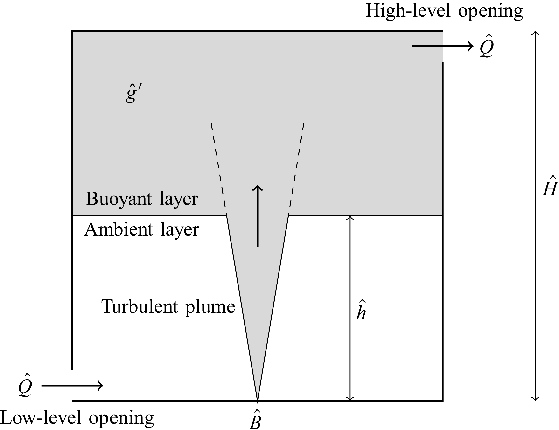
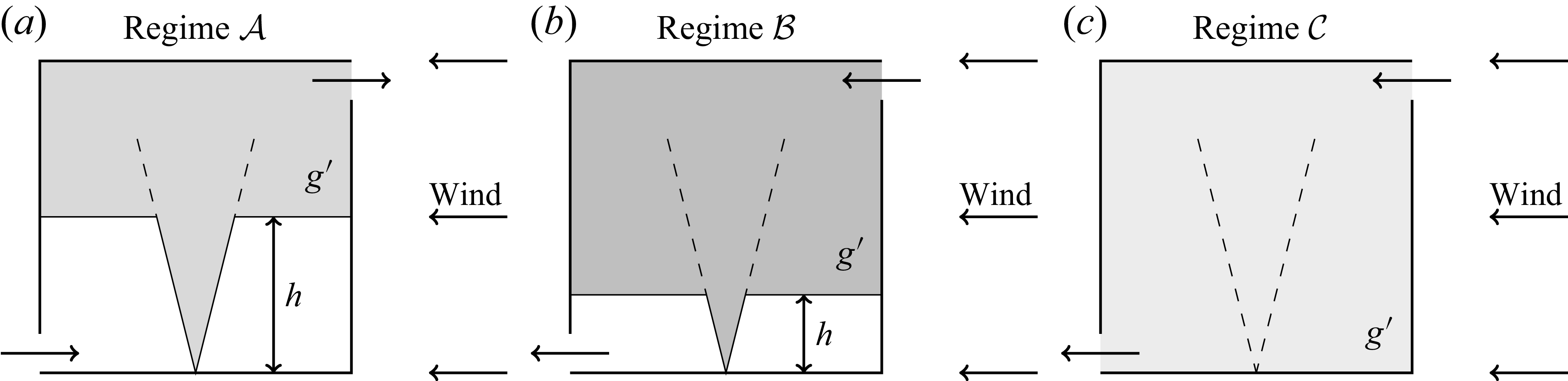


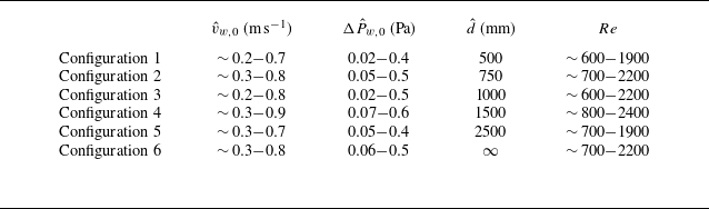


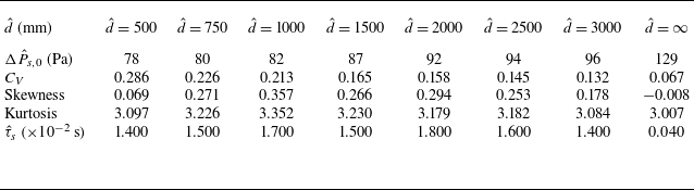

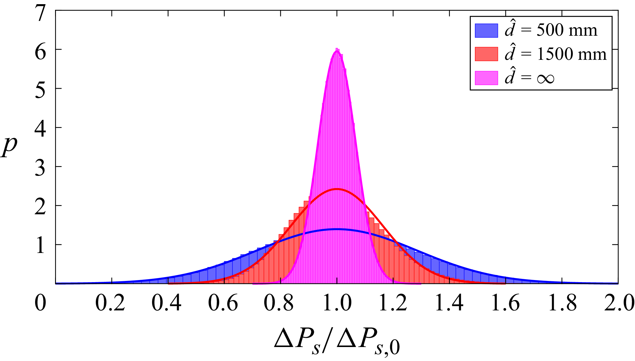


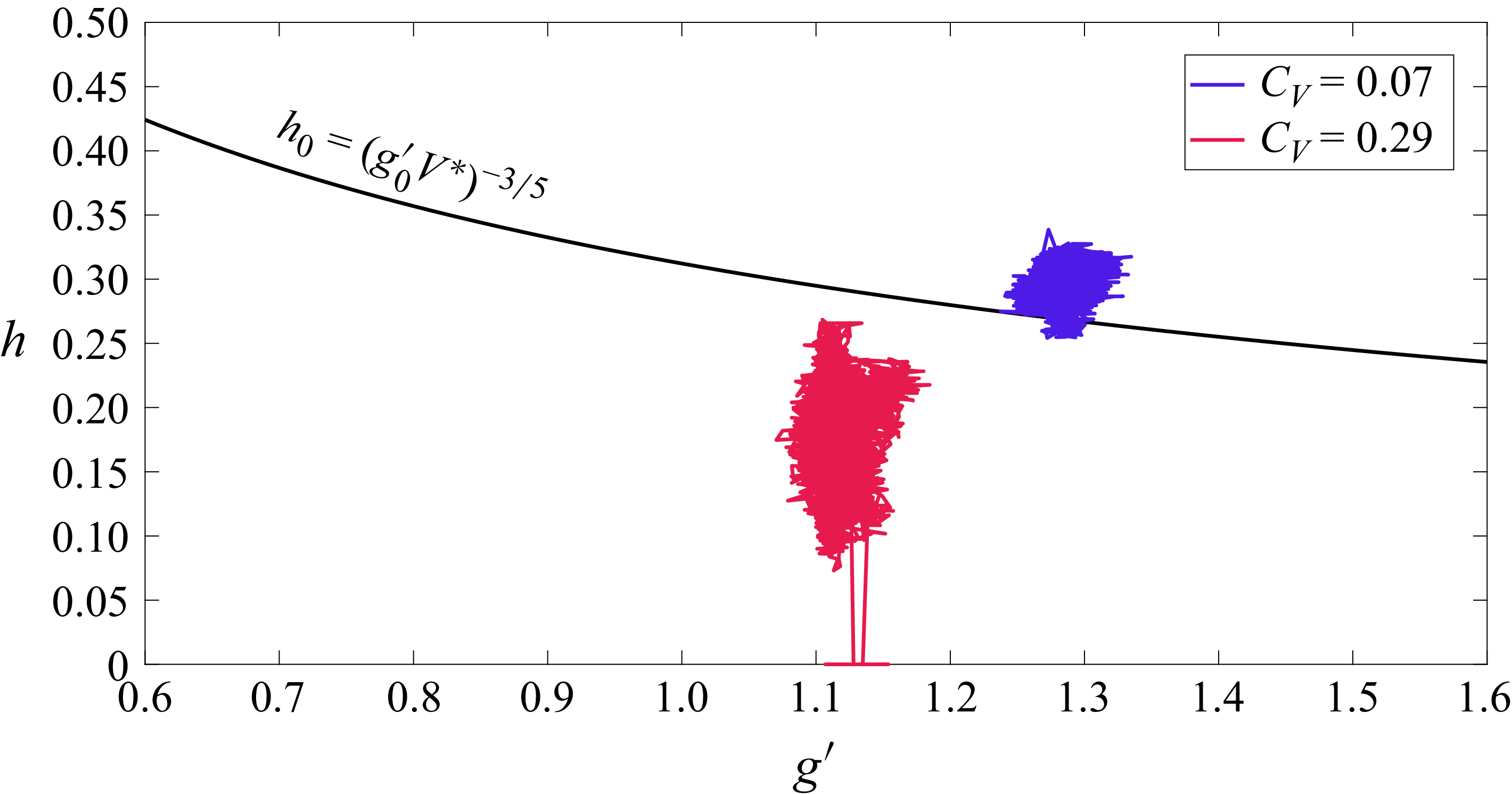


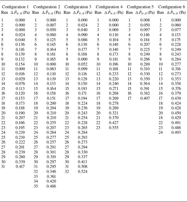


 Open access

