


1. Introduction
The impact or collision of a spherical object on a surface is a problem that has been of great interest for decades. Typical examples can be found at various length scales, such as asteroid impact (Chapman & Morrison Reference Chapman and Morrison1994), drop impact (Cheng, Sun & Gordillo Reference Cheng, Sun and Gordillo2022), ball sports (Cross Reference Cross1999), collision in granular media (Andreotti, Forterre & Pouliquen Reference Andreotti, Forterre and Pouliquen2013) or suspensions, or more commonly children playing with rubber bouncing balls. Of particular interest is the restitution coefficient, defined as the ratio between the bouncing speed  $V_\infty$ and the impact speed $V_0$. An elastic collision corresponds to the case of a bouncing speed equal to the impact speed, without any loss of energy. In real impacts, various effects of the solid tend to decrease the restitution coefficient at large velocity (Johnson Reference Johnson1987) such as viscoelasticity (Falcon et al. Reference Falcon, Laroche, Fauve and Coste1998; Ramírez et al. Reference Ramírez, Pöschel, Brilliantov and Schwager1999), plastic deformations (Tabor Reference Tabor1948; Tsai & Kolsky Reference Tsai and Kolsky1967) or sphere vibrations (Hunter Reference Hunter1957; Reed Reference Reed1985; Koller & Kolsky Reference Koller and Kolsky1987). On top of these, viscous dissipation is predominant when the impact occurs in liquid environments, for instance in particle-laden flows (Brandt & Coletti Reference Brandt and Coletti2022), which has a large variety of industrial and natural applications. Most numerical models of such flows use a point-particle approximation or immersed boundary and do not resolve the flow in the lubrication layer upon collision. Instead, empirical collision laws are implemented when particles start overlapping (Brändle De Motta et al. Reference Brändle De Motta, Breugem, Gazanion, Estivalezes, Vincent and Climent2013; Costa et al. Reference Costa, Boersma, Westerweel and Breugem2015). In this paper, we aim to describe particle collisions, focusing on the canonical problem of a soft elastic sphere impacting a rigid surface in a viscous liquid.
Several experimental studies have been devoted to the individual rebound of a particle on a surface, either immersed in a liquid (Joseph et al. Reference Joseph, Zenit, Hunt and Rosenwinkel2001; Gondret, Lance & Petit Reference Gondret, Lance and Petit2002), or with a thin oil layer lubricating the surfaces (Safa & Gohar Reference Safa and Gohar1986; Barnocky & Davis Reference Barnocky and Davis1988; Kaneta et al. Reference Kaneta, Ozaki, Nishikawa and Guo2007). Head-on and oblique particle–particle collisions have also been investigated, and follow a similar phenomenology (Joseph & Hunt Reference Joseph and Hunt2004; Yang & Hunt Reference Yang and Hunt2006). The restitution coefficient increases with increasing velocity, as the contact time decreases and the viscous friction dissipates less energy (see figure 1b). Remarkably, for a large variety of sphere sizes, material properties and fluid viscosities, the restitution coefficients collapse when plotted versus the Stokes number  ${St} = m V_0 / (6{\rm \pi} \eta R^2)$, where $m$,
$m$,  $V_0$, $\eta$ and $R$ are the sphere mass, impact velocity, viscosity and sphere radius. The Stokes number needs to exceed a critical number, which is of order $10$, for bouncing to occur. Then the restitution coefficient increases and reaches unity asymptotically when the Stokes number is ${\sim }1000$. An empirical expression $V_\infty /V_0 = \exp (-35/{St})$ has been shown to describe fairly well the experimental data over the entire range of $St$ (Legendre, Daniel & Guiraud Reference Legendre, Daniel and Guiraud2005; see green dashed lines in figure 1b), and is motivated by an analogy with a damped spring–mass model.
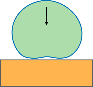
(a) Schematic of an elastohydrodynamic bouncing of a soft sphere on a rigid surface. The undeformed sphere is indicated with red dashed lines. A thin film of thickness  $h(r,t)$ prevents direct contact, where $r$ denotes the axisymmetric radial coordinate. The grey rectangle indicates a zoom in the contact region. (b) Bouncing velocity as a function of the Stokes number measured in the experiments of Gondret et al. (Reference Gondret, Lance and Petit2002), in the numerical simulations and predicted by the asymptotic theory of (6.6). The prediction of Legendre et al. (Reference Legendre, Daniel and Guiraud2005) using a linear damped mass–spring model is shown with green dashed lines.

The bouncing dynamics is modelled mainly in two ways. First, reduced linear damped mass–spring models have been introduced (Legendre et al. Reference Legendre, Daniel and Guiraud2005). The nonlinearities of the contact elasticity (Schwager & Pöschel Reference Schwager and Pöschel1998) and gravitational effects (Falcon et al. Reference Falcon, Laroche, Fauve and Coste1998) have also been taken into account. The second kind of models described the morphology of the lubrication layer upon contact. Davis, Serayssol & Hinch (Reference Davis, Serayssol and Hinch1986) were the first to derive an elastohydrodynamic lubrication model, which describes the intricate coupling between the thin liquid film and elastic deformations, when particles move near soft interfaces. The lubrication forces prevent the direct contact between the sphere and the rigid surface, such that a thin liquid film always separates the two surfaces. These models allow for a prediction of the critical bouncing Stokes number, which typically takes the form  $\ln (H/\delta )$, where $H$ is the initial separation distance, and $\delta$ is a cut-off length. The cut-off length is an elastohydrodynamic length for smooth surfaces, or the typical roughness for rough surfaces (Barnocky & Davis Reference Barnocky and Davis1988; Yang & Hunt Reference Yang and Hunt2008). Piezoviscous and compressible effects, which play an important role in lubricants, have also been discussed (Barnocky & Davis Reference Barnocky and Davis1989; Wang, Venner & Lubrecht Reference Wang, Venner and Lubrecht2013; Venner, Wang & Lubrecht Reference Venner, Wang and Lubrecht2016). We also point out that the elastohydrodynamic coupling gives rise to a very rich phenomenology for particle sliding and rotating near soft interfaces (Salez & Mahadevan Reference Salez and Mahadevan2015).
The morphology of the lubrication layer during the contact has rarely been addressed (Lian, Adams & Thornton Reference Lian, Adams and Thornton1996). The central film thickness has been identified to scale as  ${St}^{-1/2}$ in Venner et al. (Reference Venner, Wang and Lubrecht2016), suggesting the presence of self-similar solutions. We present in this paper a detailed numerical and asymptotic analysis of the elastohydrodynamic bouncing. The Stokes number is set in the range $[10, 10^4]$ in the numerical simulations of this paper, which corresponds to the relevant experimental range (see figure 1b). The structure of the lubrication layer during the impact dynamics is derived through self-similar solutions. Furthermore, the energy budget allows us to find an asymptotic expression of the restitution coefficient at large Stokes number.
2. Soft lubrication model
2.1. Formulation
We briefly recall here the soft lubrication model, already employed to model the bouncing of a sphere of radius  $R$ and mass $m$ on a rigid planar surface (Davis et al. Reference Davis, Serayssol and Hinch1986; Venner et al. Reference Venner, Wang and Lubrecht2016; Tan, Wang & Frechette Reference Tan, Wang and Frechette2019). We assume an impact normal to the surface such that the problem is axisymmetric, where the axis of symmetry is the sphere axis normal to the surface, referred to later as vertical direction ( $z$ in figure 1a). We introduce the polar coordinates where the radial position is denoted $r$. The centre of mass vertical position of the sphere, shifted by one radius, is denoted $D(t)$ (see figure 1a). We suppose that the sphere is submerged in a viscous fluid of viscosity $\eta$. Due to lubrication forces, a thin film of liquid always separates the sphere from the surface, and there is no direct contact. Using Newton's second law along the vertical direction, the sphere's dynamical equation is $m\,\dot {V}(t) = F(t)$, where $F(t)$ is the the vertical hydrodynamic viscous force acting on the particle, and $V(t) = \dot {D}(t)$ is its vertical velocity. We focus here on the contact dynamics, such that the sphere is close enough to the surface to use the lubrication approximation. Therefore, the flow in the liquid gap is a parabolic Poiseuille flow, and the liquid film thickness $h(r,t)$ follows the thin-film equation
 \begin{equation} \frac{\partial h(r,t)}{\partial t} = \frac{1}{12\eta r}\,\frac{\partial }{\partial r} \left(r\, h^3(r,t)\,\frac{\partial p(r,t)}{\partial r}\right), \end{equation}
where  $p(r,t)$ is the pressure field. Within the lubrication approximation, the contribution of the outer region of the contact to the hydrodynamic viscous force is negligible, and the hydrodynamic viscous force comes mainly from the contact region and follows the lubrication force as $F(t) = \int _0^\infty p(r,t)\,2{\rm \pi} r \,\mathrm {d}r$. Additionally, the sphere being very close to the surface, the undeformed spherical particle can be modelled with a parabolic approximation such that the liquid gap can be written as (Rallabandi Reference Rallabandi2024)
 \begin{equation} h(r,t) = D(t) + \frac{r^2}{2R} - w(r,t), \end{equation}
where  $w(r,t)$ represents the elastic deformations (see figure 1a). These deformations are modelled by using the linear elasticity theory, and are related to the pressure field with a convolution integral involving the elastic Green's function. Integrating the convolution integral in the azimuthal direction leads to the integral relation (Davis et al. Reference Davis, Serayssol and Hinch1986)
 \begin{equation} w(r,t) ={-}\frac{4}{{\rm \pi} E^*}\int_0^\infty \mathcal{M}(r,x)\,p(x,t) \, \mathrm{d} x, \quad \mathcal{M}(r,x) = \frac{x}{r+x}\,K\left(\frac{4rx}{(r+x)^2}\right), \end{equation}
where  $E^* = E/(1-\nu ^2)$ is the plane strain elastic modulus, with $E$ and $\nu$ the Young's modulus and Poisson ratio, respectively. The function $K$ is the complete elliptic integral of the first kind.
We introduce the typical sphere elastic deformation length  $D_0$ during the contact,
 \begin{equation} D_0 = \left(\frac{mV_0^2}{E^*\sqrt{R}}\right)^{2/5}, \end{equation}
obtained by balancing the kinetic energy  $mV_0^2$ with the Hertz elastic energy $E^*\sqrt {R}\,D_0^{5/2}$ (see below). Equations (2.1)–(2.3a,b) are made dimensionless by using the scales of the Hertz theory, respectively $D_0$, $\sqrt {RD_0}$, $D_0/V_0$, $p_0 = 2E^* \sqrt {D_0/R}/{\rm \pi}$ and $F_0 = p_0 RD_0$ as vertical/radial length, time, pressure and force scales, as detailed in Appendix A. We then solved numerically the resulting equations using the finite-difference scheme proposed in Liu et al. (Reference Liu, Dong, Jagota and Hui2022), as discussed in Appendix B. As an initial condition, we suppose that the sphere's position is at height $D_0$ with downward velocity $V_0$. A single dimensionless number characterizes the bouncing dynamics, which is the Stokes number
 \begin{equation} {St} = \frac{mV_0}{6{\rm \pi} \eta R^2}. \end{equation}
The Stokes number can be interpreted as the ratio between sphere inertia ( $m V_0^2$) and viscous dissipation ( $6{\rm \pi} \eta R^2V_0$), or alternatively the viscous dissipation time scale $mD_0/(6{\rm \pi} \eta R^2)$ and the bouncing time scale $D_0/V_0$. For small Stokes number (large viscosity), or dissipation time smaller than the bouncing time, the sphere does not bounce as the entire initial kinetic energy is dissipated before contact. Therefore, in the context of bouncing, the Stokes number offers a quantification of the viscous dissipation during bouncing. The critical Stokes number for bouncing to occur depends slightly on the initial altitude and is typically of order $10$ (Davis et al. Reference Davis, Serayssol and Hinch1986) (see figure 1b). In this paper, we focus on the intermediate to large Stokes number regime (low viscosity fluid), when the sphere bounces with a non-zero speed. We neglect the buoyancy forces here that do not influence the contact dynamics as long as the work done by buoyancy during contact, $\Delta \rho \,R^3 g D_0$, is small compare to the kinetic energy $mV_0^2$ (Falcon et al. Reference Falcon, Laroche, Fauve and Coste1998), where $\Delta \rho$ is the density difference between the sphere and the fluid. Finally, we suppose that the impact speed is not too large, such that the typical sphere deformation $D_0$ is small compared to the sphere radius, corresponding to the condition $(mV_0^2/(E^* R^3))^{2/5} \ll 1$.
In the following sections, we will find various asymptotic similarity solutions for the film thickness, each with a specific scale different from the typical deformation  $D_0$ (see (2.4)). We will notice that in the infinite Stokes limit, the elastohydrodynamic model converges towards the elastic collision, where the bouncing velocity is equal to the impact velocity, as discussed in the next section.
3. Impact dynamics
3.1. Dry limit,  ${St}\to \infty$: Hertz theory

In the absence of any surrounding fluid, or for  ${St}\to \infty$, an exact solution of the elastic bouncing dynamics has been introduced previously (Hertz Reference Hertz1881; Johnson Reference Johnson1987). The vertical force acting on the sphere is zero as long as the sphere is out of contact, i.e. $D(t)>0$. During the contact phase, the force follows the Hertz theory $4E^* R^{1/2}\,\delta ^{3/2}(t)/3$, where we introduce $\delta (t) = -D(t)$ as the (positive) indentation. Substituting this expression in Newton's second law for the sphere, the indentation follows the ordinary differential equation
 \begin{equation} m\,\ddot{\delta}(t) ={-}\frac{4E^*}{3}\,R^{1/2}\,\delta^{3/2}(t), \quad \text{for }\delta(t) >0, \end{equation}
which corresponds to a nonlinear mass–spring equation, where the spring stiffness increases with the indentation as  $\sqrt {\delta }$. An exact solution of (3.1) can be expressed in the form of an implicit equation
 \begin{equation} \int_0^{\delta/D_0} \frac{\mathrm{d} x}{\sqrt{1-\tfrac{16}{15}\,x^{5/2}}} = {}_2F_1\left(\frac{2}{5},\frac{1}{2};\frac{7}{5};\frac{16 (\delta(t)/D_0)^{5/2}}{15}\right) \frac{\delta(t)}{D_0} = \frac{V_0t}{D_0}, \end{equation}
where  $_2F_1$ is the hypergeometric function. We notice that the equivalent dynamical law for a linear spring model is $\arcsin (\delta (t)/D_0) = V_0t/D_0$, a solution of (3.2) if one replaces $16/15x^{5/2}$ by $x^2$ in the integral. The shape of (3.2) is fairly similar to the usual sinusoidal law for harmonic oscillators. Furthermore, the Hertz theory predicts that the pressure and elastic deformations are piecewise-defined functions that read
 \begin{gather} p_{Hz}(r,t) = \left\{\begin{array}{@{}ll} \dfrac{2E^*}{{\rm \pi} R}\,\sqrt{a^2(t)-r^2}, & r< a(t), \\ 0, & r>a(t), \end{array}\right. \end{gather}
 \begin{gather}w_{Hz}(r,t) = \left\{\begin{array}{@{}ll} -\delta(t) + \dfrac{r^2}{2R}, & r< a(t), \\ - \dfrac{1}{{\rm \pi} R}\left[(2a^2(t)-r^2)\arcsin\left(\dfrac{a(t)}{r}\right)+a(t)\,\sqrt{r^2-a^2(t)}\right], & r>a(t), \end{array}\right. \end{gather}
where  $a(t) = \sqrt {\delta (t) R}$ is the contact radius. Equations (3.3) are solutions of the elasticity equation (2.3a,b), satisfying the boundary conditions of the Hertz contact problem: (i) stress-free condition outside the contact area $r>a$, and (ii) imposed elastic deformations in the contact zone $r< a$ with a parabolic shape. Injecting the Hertz elastic deformation in the film thickness definition (2.2), we can express the film thickness predicted by the Hertz theory as
 \begin{equation} h_{Hz}(r,t) = \left\{\begin{array}{@{}ll} 0, & r< a(t), \\ -\delta(t) + \dfrac{r^2}{2R} + \dfrac{1}{{\rm \pi} R}\left[(2a^2(t)-r^2)\arcsin\left(\dfrac{a(t)}{r}\right)\right. & \\ \qquad \left.{}+a(t)\,\sqrt{r^2-a^2(t)}\vphantom{\dfrac{a(t)}{r}}\right], & r>a(t), \end{array}\right. \end{equation}
which is indeed zero within the contact zone  $r< a(t)$. The limiting behaviour of the Hertz pressure and film thickness in the vicinity of the contact radius is given by
 \begin{equation} h_{Hz}(r\to a^+) = \frac{8\sqrt{2}\sqrt{a(t)}}{3{\rm \pi} R} \left(r-a(t)\right)^{3/2}, \quad p_{Hz}(r\to a^-) = \frac{2E^*}{{\rm \pi} R}\,\sqrt{2a(t)} \left(a(t)-r\right)^{1/2}. \end{equation}
All these results will turn out to be relevant as ‘outer solutions’ for the impact dynamics at finite Stokes number.
3.2. Finite Stokes number
The bouncing dynamics at finite Stokes number is illustrated in figure 2(a) (see also supplementary movie 1, available at https://doi.org/10.1017/jfm.2024.310) for  ${St} = 100$, corresponding to the numerical solution of (2.1)–(2.3a,b). We identify five different stages during the bouncing, namely the approach, spreading, retraction, adhesion and bouncing phases. These are illustrated in figure 2(a), where we also introduce times $t_i$, for $i\in [1,5]$, that separate the phases. Initially, the sphere approaches the surface and the elastic deformation remains small, i.e. of order ${St}^{-1}$. After the time of contact $t_1 = D_0/V_0$, where the sphere would have touched the surface in the absence of surrounding fluid, the elastic deformation gradually increases as if the sphere spreads on the surface. The sphere reaches its maximal deformation at time $t=t_2$, and its vertical velocity then changes sign such that the contact radius now retracts. The time $t=t_3$ corresponds to the instant where the lubrication force vanishes, and is followed by a phase where a negative force is exerted on the sphere such that the sphere effectively adheres to the surface. Finally, at $t_4$, the sphere takes off and enters the bouncing phase, where the elastic deformations are small. We define $t_4$ empirically as the local inflexion point of the total energy of the system versus time curve, which turns out to be a good estimation of the take-off time. The fifth time, $t_5$, is defined as the time at which the sphere returns to its original altitude and bouncing velocity $V_\infty = V(t_5)$.
Bouncing dynamics. (a) Snapshots of the soft sphere interface during bouncing, which illustrates the different phases of the dynamics. The dimensionless times from left to right are  $V_0 t/D_0 = 0.8, 1.2, 2.0, 2.8, 3.5, 4.1, 4.3$, and the Stokes number is $100$. Variation of (b) the dimensionless sphere centre of mass position, (c) velocity and (d) lubrication force, versus the dimensionless time for two Stokes numbers ${St} = 50$ and $200$. The black dashed lines indicate the Hertz theory (3.2), corresponding to the absence of viscous dissipation ( ${St} = \infty$). The points illustrate the five characteristic times separating the different phases for the case ${St} = 50$ (see the definition in the text). The inset in (d) displays a zoom on the viscous adhesion phase, where the horizontal and vertical axes are rescaled with ${St}^{-2/5}$ and ${St}^{-3/5}$, respectively. We also point out that the origin of time has been shifted in the inset by $t_3$, where the force vanishes.

Figures 2(b–d) quantify the global bouncing dynamics via the sphere vertical position, velocity and lubrication force for the cases  ${St} = 50$ and $200$. The specific times $t_i$, for $i\in [1,5]$, are indicated with circles only for the case ${St} = 50$. The sphere dynamics is fairly close to the Hertz theory of (3.2) (see black dashed lines in figures 2b–d). The larger the Stokes number, the closer the dynamics to (3.2), as the viscous effects are less pronounced. Nevertheless, an important difference is that the velocity after the bounce is smaller than the impact velocity, i.e. $V_\infty /V_0 <1$, due to the presence of dissipation. Figure 1(b) displays the coefficient of restitution $V_\infty /V_0$ versus the Stokes number. The numerical results of coefficient of restitution compare fairly well with the experimental results of Gondret et al. (Reference Gondret, Lance and Petit2002) obtained for a variety of spheres of different materials/sizes and in various liquids.
A remarkable feature occurs at the end of the contact, where the lubrication force becomes negative, indicating some effective adhesion. Indeed, the sphere appears to briefly ‘stick’ to the surface (see the adhesion phase in figure 2a). We stress that there is no surface adhesion here, and the negative force arises from the viscous liquid, specifically due to the viscous resistance during the filling of the liquid gap. Hence the adhesion force here cannot be described by Johnson–Kendall–Roberts-like theory, but rather by the viscous adhesion that is also called Stefan adhesion (Wang, Feng & Frechette Reference Wang, Feng and Frechette2020). The adhesion becomes less pronounced at large Stokes number, highlighting the viscous nature of the force. Interestingly, an empirical collapse of the adhesion force is obtained when rescaling the force by  ${St}^{-3/5}$ and time by ${St}^{-2/5}$ (see inset in figure 2d), suggesting some universality of the viscous adhesion (Wang et al. Reference Wang, Feng and Frechette2020). The rescaling leads to dimensional force and time scales given respectively by $\eta R V_0 [\eta V_0 / (R E^*)]^{-2/5}$ and $R/V_0 [\eta V_0 / (R E^*)]^{2/5}$, which are mass-free and correspond to the usual elastohydrodynamic lubrication scales (see the discussion in Appendix C). A precise description of the flow and the elastohydrodynamic coupling in the adhesion phase is left for future work.
The Hertz model is dissipation-free, thus cannot predict the coefficient of restitution. To understand the viscous dissipation during bouncing, we extend the Hertz theory and analyse the lubrication film thickness during the contact. We first focus on the spreading phase of the dynamics in § 4, and the retraction phase will be discussed in § 5. The main assumption is that the Stokes number is large, so that the dynamics is close to Hertz theory.
4. Spreading phase
The film thickness and pressure profiles are shown in figures 3(a) and 3(c), respectively, for three different times during the spreading phase for the case  $St=1000$. The numerical pressure profiles agree very well with the solution of the Hertz theory (3.3) within the contact region $r< a$. Hertz theory neglects the lubrication pressure. However, the pressure gradient $\mathrm {d}p/\mathrm {d}r$ is singular at the edge of the contact radius $r=a$ (see (3.5a,b)), so that at finite velocity, the film thickness must be small in order to balance Hertz and lubrication pressures. This gives rise to small zone near the contact radius, smoothing out the pressure gradient, as shown in figure 3(c). Moreover, the liquid film profile presents a dimple shape, similar to drop impact (Josserand & Thoroddsen Reference Josserand and Thoroddsen2016), or the profiles obtained during the thin-film drainage between droplets or bubbles (Yiantsios & Davis Reference Yiantsios and Davis1990; Chan, Klaseboer & Manica Reference Chan, Klaseboer and Manica2011). We separate the theoretical analysis of the film into two zones: namely the edge of the contact called the ‘neck region’, and the central region called the ‘dimple region’ (see the schematics in figure 3).
Spreading phase: neck solution at different times. Typical dimensionless (a) film thickness and (c) pressure as functions of the dimensionless radius for three different times ( $t = 1.3, 1.5, 1.8$ times $D_0/V_0$) during the spreading phase. The Stokes number is set to $1000$. The black dashed lines show the Hertz theory. In (b,d), the profiles are rescaled by the typical length and pressure scales in the neck region, corresponding to (4.1a–d). The different lateral scales of the problem are shown in the schematic on top. The soft slider solution of Snoeijer, Eggers & Venner (Reference Snoeijer, Eggers and Venner2013) is shown with pink dashed lines.

4.1. Neck region: soft lubrication inlet analogy
The impact dynamics of a soft sphere exhibits resemblances with the problem of an elastic sphere sliding near a wall under an applied load (Venner et al. Reference Venner, Wang and Lubrecht2016). Indeed, using as a reference frame  $r\rightarrow r-a(t)$, where $a(t)$ is the contact radius of the Hertz theory, we can map the impact dynamics in the neck to the sliding of a soft sphere near a rigid wall, with a time-dependent velocity $u = \dot {a}$ and under a load $4E^* a^3 / (3R)$. In Bissett (Reference Bissett1989), Bissett & Spence (Reference Bissett and Spence1989) and Snoeijer et al. (Reference Snoeijer, Eggers and Venner2013), it has been shown that the steady soft sliding has self-similar solutions near the edge of the contact radius, which can be demonstrated rigorously using asymptotic matching methods. Here, we first recall the typical scales in the region using the scaling arguments (Snoeijer Reference Snoeijer2016). To do so, we introduce $h_n$, $\ell _n$ and $p_n$ as the typical film thickness, lateral length and pressure scales, respectively, in the neck region (see the schematic in figure 3). First, the fluid momentum balance, i.e. the Stokes equation $\eta \,\nabla ^2\boldsymbol {u} = \boldsymbol {\nabla } p$, in the horizontal direction yields $\eta u/h^{2}_n = p_n/\ell _n$ in the lubrication limit. Then, following the linear elasticity theory, the pressure is proportional to the typical strain, which reads $p_n = E^* h_n/\ell _n$. Finally, the similarity solution has to match the singular behaviour of the Hertz theory near the contact radius (see (3.5a,b)). This imposes the geometric condition $h_n = a^{1/2} \ell _n^{3/2}/R$. Combining the aforementioned expressions, one finds
 \begin{equation} h_n = \frac{a^2}{R}\,\lambda^{3/5}, \quad \ell_n = a \lambda^{2/5}, \quad p_n = E^*\,\frac{a}{R}\, \lambda^{1/5}, \quad \lambda = \frac{\eta u R^3}{E^*a^4}. \end{equation}
The dimensionless group  $\lambda$ is the relevant elastohydrodynamic dimensionless number, which needs to be small to enforce the hierarchy of scales $h_n \ll \ell _n \ll a \ll R$ of the asymptotic expansion. Following this approach, we introduce a self-similarity ansatz of the form
 \begin{equation} h(r,t) = h_n\,\mathcal{H}(\xi), \quad p(r,t) = p_n\,\mathcal{P}(\xi), \quad \xi = \frac{r-a}{\ell_n}. \end{equation}
Substituting (4.1a–d) into (2.1), and using  $\lambda \ll 1$, one gets
 \begin{equation} \left(\frac{\dot{h}_n \ell_n}{h_n \dot{a}}\,\mathcal{H} - \frac{\dot{\ell}_n}{\dot{a}}\,\xi \mathcal{H}' \right) - \mathcal{H}' = \frac{1}{12}(\mathcal{H}^3\mathcal{P}')', \end{equation}
where the term in parentheses on the left-hand side of (4.3) reflects the unsteadiness of the problem, given that both the velocity and load are time-dependent. In the early times after contact, i.e. when  $t-t_1$ is small, the vertical velocity is approximately constant, $V \approx -V_0$, such that the contact radius dynamics is governed by $a(t) \approx \sqrt {R V_0(t-t_1)}$ and $u(t) \approx \sqrt {R V_0/[4(t-t_1)]}$. Hence the elastohydrodynamic parameter, which scales as $\lambda \propto (u/a^4)\propto (t-t_1)^{-5/2}$, diverges as $t\to t_1$. The steady similarity solution develops after a transient regime, once $\lambda \ll 1$. The typical scale of the transient time can be estimated as the one when $\lambda = 1$, leading to $(t-t_1) \sim (D_0/V_0)\,{St}^{-2/5}$, which is much smaller than the bouncing time scale $D_0/V_0$ in the large ${St}$ limit. We recover the elastohydrodynamic lubrication time scales, also governing the adhesion phase (see Appendix C). Hence after this very brief transient state, the unsteady terms of (4.3) are negligible and we can integrate to obtain
 \begin{equation} \mathcal{P}' = 12\,\frac{\mathcal{H}_0-\mathcal{H}}{\mathcal{H}^3}, \end{equation}
where  $\mathcal {H}_0$ is an integration constant. In the limit where the length of the neck is smaller than the contact radius, i.e. $\ell _n \ll a$, the elastic kernel $\mathcal {M}$ of (2.3a,b) reduces to the dimensionless line force Green's function $\mathcal {M}(r,r') \propto -\tfrac {1}{2} \ln |\xi -\xi '|$ (Johnson Reference Johnson1987). Taking (twice) the derivative of (2.2), and combining with the line force elastic kernel, we find
 \begin{equation} \mathcal{H}''(\xi) ={-} \frac{2}{\rm \pi} \int_\mathbb{R} \frac{\mathcal{P}'(\xi')}{\xi-\xi'} \, \mathrm{d}\xi', \end{equation}
where we assume  $\ell _n^2/(h_n R) \ll 1$, which follows from (4.1a–d). The similarity solution has to match the asymptotic behaviour of the Hertz theory near the contact radius (see (3.5a,b)). Writing the matching condition, we find
 \begin{equation} \mathcal{H}(\xi \to \infty) = \frac{8\sqrt{2}}{2{\rm \pi}}\,\xi^{3/2}, \quad \mathcal{P}(\xi \to -\infty) = \frac{2\sqrt{2}}{\rm \pi}\,(-\xi)^{1/2}. \end{equation}
Equations (4.4)–(4.6a,b) are equivalent to the equations of the steady elastohydrodynamic sliding in the inlet zone of Snoeijer et al. (Reference Snoeijer, Eggers and Venner2013), up to a trivial prefactor rescaling. As shown in figures 3(b,d), the rescaled profiles with the similarity variables of (4.1a–d) indeed collapse for different times. Furthermore, the similarity solution derived in Snoeijer et al. (Reference Snoeijer, Eggers and Venner2013) is in perfect agreement with the profile, demonstrating that the structure of the advancing neck in the bouncing problem maps perfectly to the inlet of the soft slider, in a quasi-steady fashion. It is not trivial that the advancing neck region in the bouncing problem is equivalent to the inlet of the steady soft sliding for two reasons. First, the bouncing problem is unsteady, and second, it implies normal motion of the sphere versus lateral motion for the steady soft sliding.
The analysis above shows how at a fixed Stokes number, the spreading phase can be understood in time, by the analogy with a sliding contact problem. It is also of interest to investigate the scaling of the neck thickness upon varying the Stokes number – in particular since we expect the neck to vanish in the limit  ${St} \to \infty$. In figure 4(a), we thus plot profiles at different ${St}$, at a fixed time ( $t=1.5 D_0/V_0$) during the spreading phase. As expected, the larger the Stokes number, the thinner the lubrication film and the closer it gets to the Hertz theory. The neck film thickness and lateral scales (see (4.1a–d)) can be rewritten to make the Stokes number explicit, as
 \begin{gather} \frac{h_n}{D_0} = (6{\rm \pi}\,{St})^{{-}3/5} \left(\frac{u D_0}{V_0\sqrt{RD_0}}\right)^{3/5} \left(\frac{a}{\sqrt{R D_0}}\right)^{{-}2/5}, \end{gather}
 \begin{gather}\frac{\ell_n}{\sqrt{RD_0}} = (6{\rm \pi}\,{St})^{{-}2/5} \left(\frac{u D_0}{V_0\sqrt{RD_0}}\right)^{2/5} \left(\frac{a}{\sqrt{R D_0}}\right)^{{-}3/5}. \end{gather}
Hence we find that the Stokes number scaling of the film thickness and lateral scale of the neck during the spreading phase are  ${St}^{-3/5}$ and ${St}^{-2/5}$, respectively. Rescaling the profiles of figure 4(a) with the corresponding Stokes number scaling, a collapse of film thickness profiles is indeed observed in figure 4(b) close to the neck region. Furthermore, the inset shows the film thickness at the radial position of the Hertz contact radius, which is in perfect agreement with ${St}^{-3/5}$ over the full ${St}$ range explored numerically.
Spreading phase: Stokes number scaling. (a) Typical dimensionless film thickness as a function of the dimensionless radius at  $t = 1.5 D_0/V_0$ during the spreading phase. The three colours indicate different Stokes number, respectively $50, 200, 1000$, and the black dashed lines represent the Hertz theory. In (b) (resp. (c)), the thickness profiles are rescaled by the typical length scales in the neck (resp. dimple) region. The inset shows the thickness at (b) the Hertz contact radius and (c) the central film thickness versus the Stokes number in log–log, highlighting the Stokes number scaling with a fitted line.

4.2. Central region: dimple height model
Towards the dimple region, the neck similarity solutions deviates from the steady elastohydrodynamic inlet (see figure 3b), which has uniform thickness. Instead, in the bouncing problem, the film thickness has some spatial variations in the central region, taking the form of a dimple. The central region is not described by the same scaling laws as the neck region, and a different analysis must be adopted. We focus on the central height of the film  $h_0(t) = h(r \to 0,t)$, which is referred to as the dimple height in what follows. Figure 5(a) reports the dimple height as a function of time for various Stokes numbers. As discussed above, the larger the Stokes number and the smaller the film thickness, as the lubrication pressure gets smaller. Interestingly, the dimple heights for different Stokes numbers collapse when rescaled by ${St}^{-1/2}$ (see figure 5b). In figure 4(c), we show the radial dependence of the film thickness profiles rescaled by ${St}^{-1/2}$, where the profiles indeed collapse near the centre. Nevertheless, the profiles deviate away from the symmetry axis. Therefore, the $D_0 {St}^{-1/2}$ thickness scale is valid only in the vicinity of the symmetry axis, and does not collapse the film thickness in the entire dimple.
Dimple height. (a) Rescaled central film thickness height  $h_0(t) = h(r=0,t)$ as a function of time in both the spreading and retraction phases. The colours indicate different Stokes numbers (same as in figure 4), respectively $50$,
$50$,  $200$ and $1000$ from light to dark blue. As in figure 2, the dots indicate the times separating the different phases of the bouncing dynamics. (b) The same data with the vertical axis rescaled by ${St}^{-1/2}$. The prediction of the dimple height (4.9) is shown in a red dashed line, and the small time-to-contact asymptotic (4.10) is displayed in a yellow dotted line.

We turn to an analysis of the dimple height. The pressure field is well described by the Hertz profile (3.3a) (see figure 3c). Injecting the Hertzian pressure field in the thin-film equation (2.1) and investigating the limit  $r \to 0$, we obtain an ordinary differential equation for $h_0(t)$ as
 \begin{equation} \left.\frac{\partial h(r,t)}{\partial t}\right|_{r\to 0} = \frac{\mathrm{d}h_0(t)}{\mathrm{d}t} = \left. \frac{1}{12\eta r}\,\frac{\partial }{\partial r} \left(r\,h^3(r,t)\,\frac{\partial p_{Hz}(r,t)}{\partial r}\right) \right|_{r\to 0} ={-} \frac{E^* }{3{\rm \pi} \eta R }\, \frac{h_0^3(t)}{a(t)}. \end{equation}
Solving this equation with the initial condition  $h_0(t\to t_1^+) = \infty$, we get
 \begin{equation} h_0(t) = \left( \frac{2E^* }{3{\rm \pi} \eta R } \int_{t_1}^t \frac{\mathrm{d}\hat{t}}{a(\hat{t})}\right)^{{-}1/2} = D_0\,{St}^{{-}1/2} \left( 4\int_{Vt_1/D_0}^{Vt/D_0} \frac{\mathrm{d}\hat{t}}{a(\hat{t})/\sqrt{RD_0}}\right)^{{-}1/2}. \end{equation}
Not only do we recover the  ${St}^{-1/2}$ scaling, but the dynamics of the dimple height is described quantitatively by (4.9), as shown in figure 5(b). At small time-to-contact, i.e. $t-t_1 \ll D_0/V_0$, the Hertz contact radius follows $a(t) = \sqrt {RV_0(t-t_1)}$. In this limit, the dimple height expression simplifies to
 \begin{equation} h_0(t) \approx \left( \frac{4E^* }{3{\rm \pi} \eta R^{3/2}V_0^{1/2} }\,(t-t_1)^{1/2}\right)^{{-}1/2} \propto (t-t_1)^{{-}1/4}. \end{equation}
Interestingly, the small time-to-contact asymptotic expression provides an excellent description of the full expression, as shown with the yellow dotted line in figure 5(b). We point out that the  $-1/2$ scaling in Stokes number of the dimple height has already been discussed by Venner et al. (Reference Venner, Wang and Lubrecht2016).
5. Retraction phase
We now turn to the retraction phase of the bouncing dynamics, when the sphere vertical velocity is positive. Figure 6 displays the film thickness and pressure profiles at various times during the retraction phase. The neck appears to be translated with minor changes of its vertical or lateral scales, which differs qualitatively from the spreading phase (see figure 3a). The central region is fairly flat, as if the dimple has disappeared and the central thickness decreases very slowly in time, following (4.9).
Retraction phase. Typical dimensionless (a) film thickness and (c) pressure as functions of the dimensionless radius for three different times ( $t = 2.9, 3.2, 3.5$ times $D_0/V_0$) during the retraction phase, using the same notations as in figure 3. In (b,d), the profiles are rescaled by the typical length and pressure scales in the neck during the retraction phase, corresponding to (5.1a–c). In contrast to the spreading phase, there is no universal behaviour, although the collapse is fairly good.

Given the striking agreement between the neck region in the spreading phase and the soft slider inlet, we use the same approach to the retraction phase. The contact radius is now receding, such that the analogy must involve the outlet region of the soft slider. We stress that the central region of the soft slider has a uniform film thickness  $\mathcal {H}_0 h_n$ that is universal and selected by the inlet profile, where $\mathcal {H}_0 =2.478\ldots$ is a numerical prefactor (Snoeijer et al. Reference Snoeijer, Eggers and Venner2013). For the soft slider, the very same scaling arguments of § 4.1 still apply in the outlet, and a similarity solution can be found with the same scales as (4.1a–d). For the impact, however, the situation is different: rescaling the numerical profiles in the neck with the scales (4.1a–d) does not collapse the data during the retraction phase. For instance, figure 7(a) shows film thickness profiles at a fixed time $t = 3.2 D_0/V_0$ for various Stokes numbers. The data are rescaled in figure 7(b) in the same manner as in the spreading phase (see figure 4b), where we no longer observe a perfect collapse. The difference is further illustrated in figure 7(c), where the value of the film thickness at the Hertz contact radius is displayed versus the Stokes number in log–log scale. In the range explored numerically, the film thickness does not follow the ${St}^{-3/5}$ scaling as in the spreading phase, but is closer to the ${St}^{-1/2}$ scaling of the dimple.
Retraction phase: Stokes number scaling. (a) Typical dimensionless film thickness as a function of the dimensionless radius at  $t = 3.2 D_0/V_0$ during the spreading phase. The four colours indicate different Stokes numbers, respectively $50, 200, 1000, 10\,000$, and the black dashed lines represent the Hertz theory. (b) The thickness profiles rescaled by the typical length scales in the neck region during the spreading phase (see figure 4). (c) The thickness at the Hertz contact radius versus the Stokes number in log–log. The two lines indicate power laws with exponents $-3/5$ and $-1/2$, respectively.

The fundamental difference between the inlet and outlet solutions of the soft slider is that the inlet has a unique solution with a universal dimensionless flux  $\mathcal {H}_0$, while the outlet solution has a family of solutions with varying fluxes, where the adopted self-similar shape is found by matching to the central region thickness (Snoeijer et al. Reference Snoeijer, Eggers and Venner2013). We note that such a qualitative feature is also found in the Bretherton bubbles in a tube (Bretherton Reference Bretherton1961), where the film thickness is selected from the universal solution in the front dynamical meniscus, while the rear adopts the same self-similarity but where the solution is non-unique and selected by matching the film thickness to the central solution. Hence we conjecture that the typical thickness scale of the neck region in the retraction phase is selected by the matching to the central film thickness $h_0$, and not by the elastohydrodynamic film thickness $h_n$. As a result, the similarity solution is no longer universal and depends on a dimensionless number that is the instantaneous ratio between these two thicknesses, $h_0/h_n$, that is actually large given the ${St}$ scaling. For ${St} = 10^3$, we observed numerically that the central film thickness in the retraction phase is roughly constant in time and scales as $h_0 \sim D_0\,{St}^{-1/2}$ (see figure 6a). Hence we suppose that the film thickness scale in the neck region during the retraction is $h_r = D_0\,{St}^{-1/2}$, where the subscript $r$ stands for retraction. As in § 4.1, we invoke the matching condition of the retracting neck solution to the singular behaviour of Hertz theory (see (3.5a,b)) to determine the lateral length and pressure scales in the neck as $h_r = \ell ^{3/2}_r a^{1/2}/R$ and $p_r = E^* a^{1/2}\ell _r^{1/2}/R$. Combining the latter expressions, we find the scales
 \begin{equation} h_r = D_0\,{St}^{{-}1/2}, \quad \ell_r = \sqrt{RD_0}\,{St}^{{-}1/3} \left(\frac{a}{\sqrt{RD_0}}\right)^{{-}1/3}, \quad p_r = p_0\,{St}^{{-}1/6} \left(\frac{a}{\sqrt{RD_0}}\right)^{1/3}. \end{equation}
Once rescaled with (5.1a–c), the thickness and pressure fields in the neck collapse fairly well, as shown in figures 6(b,d). Nevertheless, as expected, there is no clear universal self-similar solution, and some details of the profiles are not described by the rescaling. Further investigations would be necessary to determine the exact asymptotic structure of the solution at large Stokes number. Such an analysis would required a Stokes number much larger than  $10^5$ in order to distinguish between the two exponents.
6. Energy dissipation and coefficient of restitution
Having discussed in detail the evolution of the lubrication film during the contact dynamics, we now investigate the bouncing restitution coefficient. To predict the restitution coefficient, we analyse the energy budget during bouncing. The only source of dissipation comes from the liquid viscosity, such that the energy dissipation rate is given by
 \begin{equation} \frac{\mathrm{d}E}{\mathrm{d}t} ={-}\int_{\mathbb{R}^3} \eta (\boldsymbol{\nabla} v)^2 \, \mathrm{d}^3x ={-} \int_{\mathbb{R}^2} \frac{h^3}{12\eta}\,(\boldsymbol{\nabla} p )^2 \, \mathrm{d}^2x, \end{equation}
where the total viscous dissipation in (6.1) is simplified to keep the dominant term within the lubrication approximation (see Appendix C in Bertin et al. Reference Bertin, Lee, Salez, Raphaël and Dalnoki-Veress2021). The total energy of the system, including kinetic energy and elastic energy of the sphere, is denoted  $E$ and is shown in figure 8(a). Interestingly, the amount of energy dissipated in each phase of the dynamics is of the same order of magnitude, which motivates a model accounting for all the phases of the bouncing dynamics. We define the energy dissipated in each phase of the dynamics by $\Delta E_i = E(t_{i})-E(t_{i-1})$, for $i \in [1, 5]$ and where $t_0 = 0$, and aim to describe the asymptotic behaviour of each phase in the large ${St}$ limit.
Energy budget. (a) Decay of the rescaled total energy of the sphere as a function of the dimensionless time. The colours indicate different Stokes numbers (same as in figure 4), respectively  $50$,
$50$,  $200$ and $1000$ from light to dark blue. The energy dissipated in each phase is denoted $\Delta E_i$, for $i \in [1, 5]$, and shown in (b–f) as functions of the Stokes number. The black dashed lines correspond to the fit of the numerical data with the asymptotic predictions in the large Stokes limit.

First, during the approach phase, the elastic deformations are small (see figure 2a), such that the lubrication force can be approximated by the lubrication force of rigid planar surface  $F(t) = 6{\rm \pi} \eta R^2 V_0 / D(t)$. Here, we suppose that the velocity is asymptotically equal to the impact velocity $V(t) \approx -V_0$, such that the distance decreases linearly in time, as $D(t) \approx H - V_0 t$. And we generalize the result to an arbitrary initial height (denoted $H$), which is $D_0$ in the numerical simulations of figure 8. Without elastic deformations, the energy dissipation rate can be expressed by $F(t)\,V(t) = -6{\rm \pi} \eta R^2 V_0^2 / D(t)$. Integrating the dissipation rate, we obtain the amount of energy dissipated as
 \begin{equation} \Delta E_1 = 6{\rm \pi} \eta R^2 V_0 \ln\left(\frac{H}{\delta}\right) = mV_0^2\,{St}^{{-}1} \ln\left(\frac{H}{\delta}\right), \end{equation}
where one needs to introduce a cut-off length  $\delta$, a priori unknown, to regularize the integral. Similar expressions have been derived previously (Davis et al. Reference Davis, Serayssol and Hinch1986). As shown in Appendix C, the typical film thickness scale at the transition between the approach and spreading phases is given by $D_0\, {St}^{-2/5}$, which is a good candidate for regularizing length. Hence we fit the numerical energy drop in the approach phase with an asymptotic law $mV_0^2\,{St}^{-1} \ln (A_{1}\,{St}^{2/5})$, where $A_{1}$ is a fitting constant. Excellent agreement is found with the numerical data (see figure 8b), where the fitting parameter is $A_1 = 1.71$. The same arguments can be employed for the bouncing phase, such that the energy drop should also follow the asymptotic law (6.2), but with a different cut-off length. Fitting the numerical value of $\Delta E_5$ with $mV_0^2\,{St}^{-1} \ln (A_{5}\,{St}^{2/5})$ gives excellent agreement (see figure 8f), where $A_5=0.67$.
In the spreading and retraction phase, the liquid flux is maximum in the neck region, such that the majority of the viscous dissipation occurs in this region. Estimating the viscous dissipation rate in (6.1) as  $h_{n,r}^3 (p_{n,r}/\ell _{n,r})^2 (a\ell _{n,r})/\eta$, and using the scales identified in §§ 4.1 and 5, the energy drop is asymptotically
 \begin{equation} \frac{\Delta E_2}{mV_0^2} = A_2\,{St}^{{-}4/5}, \quad \frac{\Delta E_3}{mV_0^2} = A_3\, {St}^{{-}1/2}, \end{equation}
where  $A_2,A_3$ are numerical constants. In this case, the fitting of the numerical energy drop in the range of Stokes numbers explored numerically (i.e. ${St} \in [10, 10^4]$) does not provide a very good fit. To get an approximate expression that is more accurate to describe the experimentally relevant range (see figure 1b), we fit the numerical energy drop in the range ${St} \in [10^2, 10^3]$, leaving the exponent as a fitting parameter. Very good agreement is found by using
 \begin{equation} \frac{\Delta E_2}{mV_0^2} = 1.26\,{St}^{{-}0.676}, \quad \frac{\Delta E_3}{mV_0^2} = 0.358\, {St}^{{-}0.556}, \end{equation}
as shown in figure 8. The expression (6.3a,b) should be seen not as an exact asymptotic expression, but as a power-law fit in the Stokes range  ${St} \in [10^2, 10^3]$. Indeed, the energy drop would be well described by the exponent predicted by the elastohydrodynamic soft slider solution ( ${St}^{-4/5}$, see (6.3a,b)) only when the elastohydrodynamic parameter $\lambda ^{1/5} \propto {St}^{-1/5}$ (see (4.1a–d)) is small. Such a condition is achieved for ${St} \gg 10^5$, which is outside of the range explored numerically. Additional simulations at larger Stokes number would allow us to determine the asymptotic energy drop during contact.
Finally, the viscous adhesion phase has scales that are inertia-free, i.e. independent of the mass of the sphere. Using the elastohydrodynamic scales (see Appendix C), we expect an asymptotic energy drop of the form
 \begin{equation} \frac{\Delta E_4}{mV_0^2} = A_4\,{St}^{{-}1}, \end{equation}
which is indeed mass-free. Fitting the numerical solutions of  $\Delta E_4$ with (6.5) gives very good agreement with $A_4 = 3.886$ as a fitting parameter. Then the global energy budget reads $m (V_0^2-V_\infty ^2)/2 = {\sum }_{i=1}^5 \Delta E_i$, which provides an expression for the restitution coefficient as
 \begin{equation} \frac{V_\infty}{V_0} \!=\!
\sqrt{1 - 2[{St}^{{-}1}
\ln(1.71\,{St}^{2/5}) \!+\!1.26\, {St}^{{-}0.676}\!+\!
0.358\,{St}^{{-}0.556}\!+\! 3.886\,{St}^{{-}1} \!+\! {St}^{{-}1}
\ln(0.67\,{St}^{2/5})]}.
\end{equation}
\begin{equation} \frac{V_\infty}{V_0} \!=\!
\sqrt{1 - 2[{St}^{{-}1}
\ln(1.71\,{St}^{2/5}) \!+\!1.26\, {St}^{{-}0.676}\!+\!
0.358\,{St}^{{-}0.556}\!+\! 3.886\,{St}^{{-}1} \!+\! {St}^{{-}1}
\ln(0.67\,{St}^{2/5})]}.
\end{equation}The asymptotic prediction of the restitution coefficient with the numerical data is excellent, as shown in figure 1(b), which is not surprising as it relies on successive fitting of the energy drop through the dynamics. Most importantly, it provides an asymptotic expression of the restitution coefficient at large Stokes number, highlighting the physics at each phase of the bouncing. In the experimental range of Stokes numbers (see figure 1b), the full expression is necessary to obtain a good approximation of the energy dissipated during the impact, as the energy drops in each phase are of similar magnitude (see figure 8a).
7. Conclusion
In this paper, we have performed numerical simulations and asymptotic analysis of the elastohydrodynamic bouncing of a soft sphere on a rigid surface. We have demonstrated that the lubricated film thickness has non-trivial self-similar dynamics that is analogous to the steady problem of a soft sliding sphere. Interestingly, the typical scales of the lubricated film are different in the spreading and retraction phases. The characterization of the self-similar features of the lubrication layer allows us to find an asymptotic expression of the restitution coefficient in elastohydrodynamic bouncing.
More generally, this paper provides a general framework to study the coupling between the lubrication layer and interface deformations during impacts or collisions. Our model focuses on one of the most simple systems, but many effects important in real impacts could be implemented, e.g. surface roughness (Wang & Frechette Reference Wang and Frechette2018), viscoelasticity (Pandey et al. Reference Pandey, Karpitschka, Venner and Snoeijer2016) and adhesion (Keh & Leal Reference Keh and Leal2016). An interesting extension of this work would be to consider oblique collisions (Joseph & Hunt Reference Joseph and Hunt2004; Mindlin & Deresiewicz Reference Mindlin and Deresiewicz2021) and investigate the torque generated by the shear forces during the contact. Additionally, the present framework could be extended to a large variety of systems either changing the impactor, e.g. drop impacts (Mandre, Mani & Brenner Reference Mandre, Mani and Brenner2009) or elastic capsules (Jambon-Puillet, Jones & Brun Reference Jambon-Puillet, Jones and Brun2020; Rémond et al. Reference Rémond, Dolique, Vittoz, Antony, Rinaldi, Manin and Géminard2022), or changing the impacted surface, e.g. stretched membranes (Courbin et al. Reference Courbin, Marchand, Vaziri, Ajdari and Stone2006; Verzicco & Querzoli Reference Verzicco and Querzoli2021; Agüero et al. Reference Agüero, Alventosa, Harris and Galeano-Rios2022) or liquid pool (Galeano-Rios et al. Reference Galeano-Rios, Cimpeanu, Bauman, MacEwen, Milewski and Harris2021; Alventosa, Cimpeanu & Harris Reference Alventosa, Cimpeanu and Harris2023; Sykes et al. Reference Sykes, Cimpeanu, Fudge, Castrejón-Pita and Castrejón-Pita2023).
Supplementary movie
A supplementary movie is available at https://doi.org/10.1017/jfm.2024.310.
Acknowledgements
It is a pleasure to thank P. Chantelot, J. Eggers, A. Oratis and J.H. Snoeijer for stimulating discussions, as well as D. Bonn, B. Gorin and N. Ribe for sharing unpublished experimental results that motivate this work. I also thank the anonymous referees for constructive feedback that greatly improved this paper.
Funding
I acknowledge financial support from NWO through VICI grant no. 680-47-632.
Declaration of interests
The author reports no conflict of interest.
Data availability statement
The code developed in the present paper is permanently available on GitHub (see https://github.com/vincent-bertin/elastohydrodynamic-bouncing).
Appendix A. Dimensionless equations
This appendix expands the non-dimensionalization of the soft lubrication equations (2.1)–(2.3a,b). We choose to use the typical elastic scales to make the equations dimensionless, which does not account for viscous effects. The typical elastic deformation of a sphere with an impact speed  $V_0$ follows
 \begin{equation} D_0 = \left(\frac{mV_0^2}{E^*\sqrt{R}}\right)^{2/5}, \end{equation}
obtained by balancing the kinetic energy  $mV_0^2$ with the elastic energy $E^* \sqrt {R}\,D_0^{5/2}$. Using the Hertz pressure profile, we introduce a pressure scale $p_0$ based on the typical elastic deformation as
 \begin{equation} p_0 = \frac{2E^*}{\rm \pi}\sqrt{\frac{D_0}{R}} = \frac{2E^*}{\rm \pi} \left(\frac{mV_0^2}{E^*R^3}\right)^{1/5}. \end{equation}
Hence we introduce dimensionless variables (with tildes) as
 \begin{equation} \left. \begin{gathered}
h(r,t) \!=\! D_0\,\tilde{h}(\tilde{r},\tilde{t}), \quad w(r,t)
= D_0\,\tilde{w}(\tilde{r},\tilde{t}), \quad p(r,t) \!=\!
p_0\,\tilde{p}(\tilde{r},\tilde{t}), \quad F(t) = p_0
RD_0\,\tilde{F}(\tilde{t}),\\ D(t) =
D_0\,\tilde{D}(\tilde{t}), \quad V(t) =
V_0\,\tilde{V}(\tilde{t}), \quad r =
\sqrt{RD_0}\,\tilde{r}, \quad t =
\frac{D_0}{V_0}\,\tilde{t}. \end{gathered} \right\}
\end{equation}
\begin{equation} \left. \begin{gathered}
h(r,t) \!=\! D_0\,\tilde{h}(\tilde{r},\tilde{t}), \quad w(r,t)
= D_0\,\tilde{w}(\tilde{r},\tilde{t}), \quad p(r,t) \!=\!
p_0\,\tilde{p}(\tilde{r},\tilde{t}), \quad F(t) = p_0
RD_0\,\tilde{F}(\tilde{t}),\\ D(t) =
D_0\,\tilde{D}(\tilde{t}), \quad V(t) =
V_0\,\tilde{V}(\tilde{t}), \quad r =
\sqrt{RD_0}\,\tilde{r}, \quad t =
\frac{D_0}{V_0}\,\tilde{t}. \end{gathered} \right\}
\end{equation}Substituting (A3) into (2.1)–(2.3a,b), we obtain the system of equations
 \begin{gather} \frac{\partial \tilde{h}(\tilde{r},\tilde{t})}{\partial \tilde{t}} = \frac{St}{\tilde{r}}\,\frac{\partial }{\partial \tilde{r}} \left(\tilde{r}\, \tilde{h}^3(\tilde{r},\tilde{t})\,\frac{\partial \tilde{p}(\tilde{r},\tilde{t}) }{\partial \tilde{r}}\right), \end{gather}
 \begin{gather} \tilde{h}(\tilde{r},\tilde{t}) = \tilde{D}(\tilde{t}) + \frac{\tilde{r}^2}{2} - \tilde{w}(\tilde{r},\tilde{t}), \end{gather}
 \begin{gather} \tilde{w}(\tilde{r},\tilde{t}) ={-}\frac{8}{{\rm \pi}^2}\int_0^\infty \mathcal{M}(\tilde{r},\tilde{x})\, \tilde{p}(\tilde{x},\tilde{t}) \, \mathrm{d}\tilde{x}, \quad \mathcal{M}(\tilde{r},\tilde{x}) = \frac{\tilde{x}}{\tilde{r}+\tilde{x}}\,K\left(\frac{4\tilde{r}\tilde{x}}{(\tilde{r}+\tilde{x})^2}\right), \end{gather}
 \begin{gather} \frac{\mathrm{d}\tilde{V}}{\mathrm{d}\tilde{t}}= \tilde{F}(\tilde{t}), \quad \tilde{F}(\tilde{t}) = 4\int_0^\infty \tilde{p}(\tilde{r},\tilde{t})\,\tilde{r} \,\mathrm{d}\tilde{r}, \end{gather}
 \begin{gather} \tilde{V} = \frac{\mathrm{d}\tilde{D}}{\mathrm{d}\tilde{t}}. \end{gather}
The sphere is assumed to start with an impact velocity  $V_0$ and at a distance $D_0$ from the surface, leading to the initial conditions
 \begin{equation} \tilde{D}(0) = 1, \quad \tilde{V}(0) ={-}1. \end{equation}
Initial conditions are also required for the pressure and deformation fields. A naive choice would be to set the initial pressure and deformation to zero, which leads to unphysical jumps at  $t=0^+$ that affect the approach phase. To bypass this issue, we introduce an initialization phase where the velocity is ramped from $0$ to $-V_0$ during a time $t_{ini}$, as suggested in Liu et al. (Reference Liu, Dong, Jagota and Hui2022). More precisely, the velocity and sphere position are set to
 \begin{equation} \tilde{V}(\tilde{t}) ={-}\left( 1 + \frac{\tilde{t}}{\tilde{t}_{ini}}\right), \quad \tilde{D}(\tilde{t}) = 1 -\left( \tilde{t} + \frac{\tilde{t}^2}{2\tilde{t}_{ini}}\right), \quad -\tilde{t}_{ini} \leq \tilde{t} < 0, \end{equation}
and the deformation and pressure fields are identically zero at  $\tilde {t}=-\tilde {t}_{ini}$. Then solving the initialization phase with the numerical scheme discussed in Appendix B allows us to obtain initial pressure and deformation fields $\tilde {p}(\tilde {r},0)$ and $\tilde {w}(\tilde {r},0)$. We have checked that the choice of the initialization time has negligible effects in the overall bouncing dynamics.
Appendix B. Finite-difference scheme
In this appendix, we detail the finite-difference scheme used to solve the dimensionless lubrication equations (A4). We follow the methodology introduced by Liu et al. (Reference Liu, Dong, Jagota and Hui2022). We introduce a uniform spatial grid  $\tilde {r}_i = i \,\Delta r$, for $i \in [0, N-1]$, where $\Delta r$ is the grid size, and $N$ is the number of radial points. The temporal axis is also discretized by using a constant time step $\Delta t$ as $\tilde {t}^n = n\,\Delta t$. The time step is set to $10^{-4}$ or below, which is small enough to avoid any negative values of $h$ and ensures numerical stability. Hence the pressure, film thickness and deformation fields are discretized as $\tilde {p}(\tilde {r},\tilde {t}) = \tilde {p}_i^n$, $\tilde {h}(\tilde {r},\tilde {t}) = \tilde {h}_i^n$ and $\tilde {w}(\tilde {r},\tilde {t}) = \tilde {w}_i^n$, and the velocity and sphere position are $\tilde {V} = \tilde {V}^n$ and $\tilde {D} = \tilde {D}^n$, respectively. The dimensionless thin-film equation (A4a) can be expanded as
 \begin{equation} \tilde{V} - \frac{\partial \tilde{w}(\tilde{r},\tilde{t})}{\partial t} = {St} \left[ \frac{\tilde{h}^3}{\tilde{r}}\,\frac{\partial \tilde{p}}{\partial \tilde{r}} +3\tilde{h}^2 \left(r - \frac{\partial \tilde{w}}{\partial \tilde{r}}\right) \frac{\partial \tilde{p}}{\partial \tilde{r}} + \tilde{h}^3\,\frac{\partial^2 \tilde{p}}{\partial \tilde{r}^2}\right], \end{equation}
where we used the film thickness definition (A4b). The nonlinear term  $h^3$ of the thin-film equation is evaluated at the previous time, so that we end up with a linear discrete set of equations, which greatly reduces the computational time as compared to nonlinear schemes. Furthermore, we use an implicit scheme, which provides a better numerical stability as compared to explicit methods. Hence (B1) is discretized as
 \begin{align} &\tilde{V}^{n+1} -
\frac{\tilde{w}^{n+1}_i - \tilde{w}_i^n}{\Delta t}\nonumber\\ & \quad = {St}
\left[ \frac{(\tilde{h}^{n}_i)^3}{\tilde{r}_i}
\left.\frac{\partial \tilde{p}}{\partial
\tilde{r}}\right|^{n+1}_i +3(\tilde{h}^{n}_i)^2 \left(r_i -
\left.\frac{\partial \tilde{w}}{\partial
\tilde{r}}\right|^{n}_i\right) \left.\frac{\partial
\tilde{p}}{\partial \tilde{r}}\right|^{n+1}_i +
(\tilde{h}^{n}_i)^3\left.\frac{\partial^2
\tilde{p}}{\partial \tilde{r}^2}\right|^{n+1}_i\right],
\end{align}
\begin{align} &\tilde{V}^{n+1} -
\frac{\tilde{w}^{n+1}_i - \tilde{w}_i^n}{\Delta t}\nonumber\\ & \quad = {St}
\left[ \frac{(\tilde{h}^{n}_i)^3}{\tilde{r}_i}
\left.\frac{\partial \tilde{p}}{\partial
\tilde{r}}\right|^{n+1}_i +3(\tilde{h}^{n}_i)^2 \left(r_i -
\left.\frac{\partial \tilde{w}}{\partial
\tilde{r}}\right|^{n}_i\right) \left.\frac{\partial
\tilde{p}}{\partial \tilde{r}}\right|^{n+1}_i +
(\tilde{h}^{n}_i)^3\left.\frac{\partial^2
\tilde{p}}{\partial \tilde{r}^2}\right|^{n+1}_i\right],
\end{align}
where the film thickness discretization is  $\tilde {h}^n_i = \tilde {D}^n + \tilde {r}_i^2/2 - \tilde {w}_i^n$. The first- and second-order discrete spatial derivatives of (B2) are evaluated as
 \begin{equation} \left.\frac{\partial \tilde{w}}{\partial \tilde{r}}\right|^{n}_i = \frac{\tilde{w}_{i+1}^n-\tilde{w}_{i}^n}{\Delta r}, \quad \left.\frac{\partial \tilde{p}}{\partial \tilde{r}}\right|^{n+1}_i = \frac{\tilde{p}_{i+1}^{n+1}-\tilde{p}_{i}^{n+1}}{\Delta r}, \quad \left.\frac{\partial^2 \tilde{p}}{\partial \tilde{r}^2}\right|^{n+1}_i = \frac{\tilde{p}_{i+1}^{n+1}-2\tilde{p}_{i}^{n+1}+\tilde{p}_{i-1}^{n+1}}{\Delta r^2}. \end{equation}
The thin-film equation is a second-order differential equation in the radial coordinate, so we need to introduce two boundary conditions. The symmetry condition imposes that the gradient of the pressure in the centre is null, i.e.  $({\partial \tilde {p}}/{\partial \tilde {r}})(\tilde {r}=0)=0$. Furthermore, at large radius, the pressure field decays rapidly as $r^{-4}$ from (A4a). Hence we impose the boundary conditions
 \begin{equation} p_1^{n} - p_0^n = 0, \quad p_{N-1}^n=0. \end{equation}
To evaluate the integral equation of elasticity (A4c), we suppose that the pressure field is uniform and equal to  $\tilde {p}^n_i$ on each domain $[r_i - {\Delta r}/{2}, r_i + {\Delta r}/{2}]$, for $i\geq 1$, and $p_0^n$ on the domain $[0,{\Delta r}/{2}]$ near the symmetry axis. This leads to the equation
 \begin{align} &\tilde{w}_i^n
={-}\frac{8}{{\rm \pi}^2} \left[ p_0^n \int_0^{{\Delta r}/{2}}
\frac{x}{x+\tilde{r}_i}\, K\left(\frac{4 x
\tilde{r}_i}{(x+\tilde{r}_i)^2}\right)\mathrm{d} x\right.\nonumber\\ &\left.\quad +\,
\sum_{i=1}^{N-1} p_i^n\int_{\tilde{r}_i-{\Delta
r}/{2}}^{\tilde{r}_i+{\Delta r}/{2}}
\frac{x}{x+\tilde{r}_i}\, K\left(\frac{4 x
\tilde{r}_i}{(x+\tilde{r}_i)^2}\right)\mathrm{d} x \right].
\end{align}
\begin{align} &\tilde{w}_i^n
={-}\frac{8}{{\rm \pi}^2} \left[ p_0^n \int_0^{{\Delta r}/{2}}
\frac{x}{x+\tilde{r}_i}\, K\left(\frac{4 x
\tilde{r}_i}{(x+\tilde{r}_i)^2}\right)\mathrm{d} x\right.\nonumber\\ &\left.\quad +\,
\sum_{i=1}^{N-1} p_i^n\int_{\tilde{r}_i-{\Delta
r}/{2}}^{\tilde{r}_i+{\Delta r}/{2}}
\frac{x}{x+\tilde{r}_i}\, K\left(\frac{4 x
\tilde{r}_i}{(x+\tilde{r}_i)^2}\right)\mathrm{d} x \right].
\end{align}The integrals in (B5) are independent of the discrete fields, and depend only on the spatial grid. Therefore, they can be computed once and stored in a matrix to save some computational time. Numerically, they are evaluated with a Gaussian quadrature using the scipy integrate library in Python. Finally, Newton's second law for the sphere is discretized with a backward Euler scheme as
 \begin{equation} \frac{\tilde{V}^{n+1}-\tilde{V}^{n}}{\Delta t} = 4 \sum_{i=0}^{N-1} \tilde{p}_i^{n+1} \tilde{r}_{i}\, \Delta r, \quad \frac{\tilde{D}^{n+1}-\tilde{D}^{n}}{\Delta t} = \tilde{V}^{n+1}, \end{equation}
which completes the discrete system of equations. The code is available at the link https://github.com/vincent-bertin/elastohydrodynamic-bouncing.
Appendix C. Elastohydrodynamic lubrication scales in the adhesion phase and the transition from approach to spreading
In this appendix, we rationalize the typical scales found in the main text for both the adhesion phase (see § 3.2, and inset in figure 2d) and the transition between approach and the spreading phase (see § 4.1). The corresponding scales are denoted below with superscript stars. Both of these phases occur on time scales much smaller than the bouncing time  $D_0/V_0$. Hence the kinetic energy of the sphere does not vary significantly during these phases, and the scales must be independent of the sphere mass. The elasticity plays a role in the approach when the elastic deformations $w^*$ are comparable to the film thickness $h^*$, i.e. $h^*\sim w^*$. The film thickness scale can be found by balancing the typical lubrication pressure scale $\eta V_0 R/h^{*2}$ with the elastic pressure $E^* w^*/r^*$, where $r^*$ is the typical radial scale. The spherical shape of the film thickness in the contact region enforces the geometric relation $h^* = r^{*2}/R$. Combining these relationships, we recover the usual elastohydrodynamic lubrication scales as
 \begin{align} & w^* = h^* = R
\left(\frac{\eta V_0}{E^*R}\right)^{3/5} =
D_0\,{St}^{{-}2/5},\nonumber\\ & \quad t^* = \frac{h^*}{V_0}
= \frac{D_0}{V_0}\,{St}^{{-}2/5}, \quad F^* =
\frac{\eta R^2 V_0}{h^*} = F_0\, {St}^{{-}3/5}.
\end{align}
\begin{align} & w^* = h^* = R
\left(\frac{\eta V_0}{E^*R}\right)^{3/5} =
D_0\,{St}^{{-}2/5},\nonumber\\ & \quad t^* = \frac{h^*}{V_0}
= \frac{D_0}{V_0}\,{St}^{{-}2/5}, \quad F^* =
\frac{\eta R^2 V_0}{h^*} = F_0\, {St}^{{-}3/5}.
\end{align}
Figure 9 displays the minimum film thickness versus time, for times near the transition from approach to spreading (figure 9a) and in the adhesion phase (figure 9b). An excellent collapse of the numerical profiles is found using  $h^*$ and $t^*$ as scales, which confirms that the elastohydrodynamic lubrication scales govern the corresponding processes.
Dimensionless minimum film thickness versus the dimensionless time. In (a) (resp. (b)), the time is shifted by  $t_1$ (resp. $t_3$). The film thickness and time axis are rescaled by ${St}^{-2/5}$, corresponding to the mass-free elastohydrodynamic lubrication scales.


 Open access