


1. Introduction
Wall-bounded turbulent flows with suspended particles are ubiquitous in both natural environments and engineering applications, such as sediment transport in rivers and estuaries, atmospheric pollution control, volcanic ash plumes, cooling systems in nuclear or electronic devices, chemical reactors and slurry pipelines (Crowe Reference Crowe2005; Guha Reference Guha2008; Balachandar & Eaton Reference Balachandar and Eaton2010; Eshghinejadfard & Thévenin Reference Eshghinejadfard and Thévenin2016). In thermally modulated particle-laden flows, turbulence commonly occurs alongside vertical temperature differences, resulting in thermally stratified turbulence. Stratification, arising from density variations due to thermal or compositional gradients, plays a pivotal role in governing the stability and dynamics of buoyancy-driven flows. The phenomenon is typically classified into two basic types, stable stratification and unstable stratification, based on the vertical distribution characteristics of the fluid density gradient. In stable stratification, the fluid density decreases with increasing height, resulting in a statically stable configuration. Conversely, unstable stratification occurs when denser fluid overlies lighter fluid, leading to gravitational instability and the spontaneous development of convective motion. In stratified turbulence, the underlying mechanisms are governed by the complex interactions between turbulent flow structures and particle-induced disturbances, ultimately regulating interphase momentum and thermal energy transfer (Elghobashi Reference Elghobashi1994; Brandt & Coletti Reference Brandt and Coletti2022). Therefore, investigating the modulation of stratified turbulence by dispersed particles is fundamentally important.
Xia (Reference Xia2013) and Xia et al. (Reference Xia, Huang, Xie and Zhang2023) summarized the advancements and future directions in convective thermal turbulence. While there have been numerous studies on particle–turbulence interactions without thermal stratification (Kuerten, Van der Geld & Geurts Reference Kuerten, van der Geld and Geurts2011; Nakhaei & Lessani Reference Nakhaei and Lessani2017; Liu et al. Reference Liu, Tang, Shen and Dong2017; Ardekani et al. Reference Ardekani, Al Asmar, Picano and Brandt2018b ; Yousefi et al. Reference Yousefi, Ardekani and Brandt2020, Reference Yousefi, Ardekani, Picano and Brandt2021), emerging research has now turned to examine how inertial particles behave in thermally stratified turbulence, uncovering novel particle–fluid coupling mechanisms induced by buoyancy effects. Point-particle approximation has been widely used to investigate the particle dynamics in convective thermal turbulence (Park, O’Keefe & Richter Reference Park, O’Keefe and Richter2018; Xu et al. Reference Xu, Tao, Shi and Xi2020; Du & Yang Reference Du and Yang2022; Yang et al. Reference Yang, Wan, Zhou and Dong2022a , Reference Yang, Wang, Tang, Zhou and Dongb , Reference Yang, Zhang, Wang, Dong and Zhouc ; Denzel, Bragg & Richter Reference Denzel, Bragg and Richter2023). Oresta & Prosperetti (Reference Oresta and Prosperetti2013) and Park et al. (Reference Park, O’Keefe and Richter2018) showed that particle characteristics, especially their diameter and inertia, could considerably influence the heat transfer and the overall flow structures. Van Aartrijk & Clercx (Reference Van Aartrijk and Clercx2009) conducted direct numerical simulations to investigate the distinct dispersion patterns and statistical behaviours of inertial particles in stably stratified turbulence, as compared with isotropic turbulence. Lovecchio, Zonta & Soldati (Reference Lovecchio, Zonta and Soldati2014) investigated the dispersion of small particles in thermally stratified open-channel turbulence using direct numerical simulations and Lagrangian particle tracking. They demonstrated that thermal stratification reduced the settling velocity of floaters in the bulk flow and weakened the particle clustering at the surface. As stratification increased, the filamentary patterns seen in unstably stratified flows gradually disappeared, leading to a more uniform, nearly two-dimensional distribution. Sozza et al. (Reference Sozza, De Lillo, Musacchio and Boffetta2016) investigated the behaviour of small inertial particles in stratified turbulence, and showed that vertical confinement of particle motion was predominantly influenced by the strength of the stratification, while particle properties played only a minor role. They further observed that particle clustering at small scales exhibited a fractal structure governed primarily by the particle relaxation time. Recent works on the inertial particle transport in unstably stratified turbulent channel flows have shed light on the complex interplay between buoyancy-driven structures and dispersed phases. Pan et al. (Reference Pan, Dong, Zhou and Shen2022) examined the sedimentation of radiatively heated solid particles in Rayleigh–Bénard (RB) turbulent flow, and showed that smaller particles exhibited chaotic sedimentation, and more efficiently absorbed solar energy. Yang et al. (Reference Yang, Wan, Zhou and Dong2022a , Reference Yang, Zhang, Wang, Dong and Zhouc ) examined the modulation of RB turbulence by isothermal and radiatively heated inertial particles, respectively. Du & Yang (Reference Du and Yang2022) investigated thermal convection driven by heat-releasing point particles in wall-bounded turbulent flow and the effects of the Stokes and Rayleigh numbers on flow dynamics, particle accumulation and heat transfer. Pan et al. (Reference Pan, Shen, Zhou and Dong2025) conducted direct numerical simulations with a two-way coupled Lagrangian tracking method to study inertial particle behaviour in unstably stratified channel flows driven by mixed convection, taking into account the particle settling effects. It was observed that, compared with neutral conditions, large-scale longitudinal vortices in unstably stratified flows caused inertial particle accumulation on the cold plume side and depletion on the hot plume side, and the inertial particles reduced streamwise velocity and enhanced the symmetry of the velocity profile. Furthermore, they quantitatively analysed the heat flux associated with particles settling in stratified turbulence, focusing on their thermal absorption and the effects of buoyancy on settling and reinjection dynamics.
However, the aforementioned studies primarily rely on the point-particle approximation, which inherently neglects detailed flow dynamics at the particle scale, such as wake formation and local boundary layer separation. As the particle size departs from the idealized microscale assumptions and becomes comparable to turbulence length scales, these neglected features play a dominant role in regulating interphase transfer (Calzavarini et al. Reference Calzavarini, Volk, Bourgoin, Lévêque, Pinton and Toschi2009; Mathai et al. Reference Mathai, Prakash, Brons, Sun and Lohse2015; Uhlmann & Chouippe Reference Uhlmann and Chouippe2017). Consequently, extensive studies have been devoted to employing interface-resolved methods to elucidate how finite-size inertial particles interact with stratified wall-bounded turbulent flows. However, works focusing specifically on thermally stratified turbulent flows laden with finite-size particles remain quite limited to date.
Jang & Lee (Reference Jang and Lee2018) employed direct numerical simulation combined with a non-uniform grid immersed boundary method to investigate the effects of finite-size particles in thermally stratified wall-bounded turbulence. They showed that neutrally buoyant particles enhanced internal gravity waves, while slightly heavier particles substantially modified the turbulence structures. In addition, the particles attenuated the vertical heat transfer. Gu, Takeuchi & Kajishima (Reference Gu, Takeuchi and Kajishima2018) investigated numerically the effects of particle volume fraction on the Nusselt number at relatively low Rayleigh numbers. Gu et al. (Reference Gu, Takeuchi, Fukada and Kajishima2019) examined the flow patterns and the effect of local heat transfer for low and high heat conductivity ratios. Takeuchi et al. (Reference Takeuchi, Miyamori, Gu and Kajishima2019) investigated the impact of conductivity ratio and average interparticle spacing on the reversal events in a two-dimensional square box. Demou et al. (Reference Demou, Ardekani, Mirbod and Brandt2022) demonstrated that neutrally buoyant finite-size particles in RB convection, with thermophysical properties matching those of the fluid, enhanced heat transfer at low particle concentrations, while suppressing heat transfer at high particle volumes. Wu et al. (Reference Wu, Karzhaubayev, Shen and Wang2024) numerically simulated particle-laden RB convection with the thermal lattice-Boltzmann method, showing that the presence of finite-size solid particles increased the Nusselt number by enhancing heat flux. Chen et al. (Reference Chen, Ostilla-Mónico, Floryan, Lee and Prosperetti2025) investigated the dynamics of finite-size suspended particles in RB convection, and showed that particle deposition, resuspension and dune formation at the cell bottom significantly affected flow structure and heat transfer, though their impact on the Nusselt number was minimal. Fan et al. (Reference Fan, Xia, Lin, Guo and Yu2025) performed direct numerical simulations of RB convection laden with non-isothermal neutrally buoyant finite-size particles with a fictitious domain (FD) method, and examined the effects of solid volume fraction, thermal conductivity ratio, specific heat ratio and particle size on the heat transfer. It is worth noting that most of these finite-size particle studies are confined to RB convection which is driven purely by buoyancy. In contrast, many engineering flows involve a coupling of thermal stratification and strong mean shear. The interaction between finite-size particles and the complex coherent structures arising from this shear-buoyancy coupling remains significantly less explored compared with pure convection cases. Despite these advancements, the specific role of particle heat capacity, which governs the thermal inertia of the dispersed phase, in modulating the global heat transfer within wall-bounded shear flows has not been investigated.
To address these gaps, the present study performs interface-resolved direct numerical simulations of turbulent channel flow with unstable thermal stratification laden with finite-size particles. To the best of our knowledge, this is the first effort to elucidate the effects of finite-size particles on flow dynamics and heat transfer in this regime, with a specific focus on comparing the results with the neutral case where natural convection is absent. The rest of the paper is outlined as follows. A description of the numerical method and simulation configuration is presented in § 2. In § 3, our results are presented and discussed, including the effects of particles on flow and temperature structures, flow and temperature statistics, and budget analysis of flow drag and heat transport. Finally, in § 4, the key findings of the present study are summarized.
2. Numerical method
In the present study, the simulations of particle-laden turbulent channel flows with heat transfer are conducted with a FD method developed by Fan et al. (Reference Fan, Lin, Xu and Yu2023). In this approach, it is assumed that the particle interior is filled with fluid, and the motion of the fictitious fluid is constrained to match the particle velocity via a pseudobody force which is introduced as a distributed Lagrange multiplier (Glowinski et al. Reference Glowinski, Pan, Hesla and Joseph1999). To simplify the description, we consider just one rigid particle in a viscous incompressible fluid below.
2.1. The FD formulation for flow
The solid domain is represented as $P( t )$
, with its boundary denoted as
$P( t )$
, with its boundary denoted as $\partial P( t )$
. Let
$\partial P( t )$
. Let $\varOmega$
be the entire domain, encompassing both the internal and external regions of the particle, and
$\varOmega$
be the entire domain, encompassing both the internal and external regions of the particle, and $\varGamma$
be the boundary of
$\varGamma$
be the boundary of $\varOmega$
. A Dirichlet or adiabatic boundary condition is applied on the outer boundary
$\varOmega$
. A Dirichlet or adiabatic boundary condition is applied on the outer boundary $\varGamma$
, specifying the velocity and temperature distributions. The physical properties of particles are characterized by its volume
$\varGamma$
, specifying the velocity and temperature distributions. The physical properties of particles are characterized by its volume $V_{\!p}$
, density
$V_{\!p}$
, density $\rho _s$
, moment-of-inertia tensor
$\rho _s$
, moment-of-inertia tensor $\boldsymbol{J}$
, angular velocity
$\boldsymbol{J}$
, angular velocity $\boldsymbol{\omega }$
, translational velocity
$\boldsymbol{\omega }$
, translational velocity $\boldsymbol{U}$
, heat conductivity
$\boldsymbol{U}$
, heat conductivity $k_s$
, heat capacity
$k_s$
, heat capacity $c_{ps}$
and heat expansion coefficient
$c_{ps}$
and heat expansion coefficient $\beta _s$
. For the fluid, the relevant properties include density
$\beta _s$
. For the fluid, the relevant properties include density $\rho _{\!f}$
, viscosity
$\rho _{\!f}$
, viscosity $\mu$
, heat conductivity
$\mu$
, heat conductivity $k_{\!f}$
, heat capacity
$k_{\!f}$
, heat capacity $c_{pf}$
and heat expansion coefficient
$c_{pf}$
and heat expansion coefficient $\beta _{\!f}$
.
$\beta _{\!f}$
.
Let $T_{\!f}$
and
$T_{\!f}$
and $\rho _{\!f}$
denote the temperature and density of the fluid, respectively, and
$\rho _{\!f}$
denote the temperature and density of the fluid, respectively, and $T_s$
and
$T_s$
and $\rho _s$
represent the corresponding solid properties. The coupling between the temperature and flow fields is modelled using the Boussinesq approximation. The following scales are introduced for non-dimensionalization:
$\rho _s$
represent the corresponding solid properties. The coupling between the temperature and flow fields is modelled using the Boussinesq approximation. The following scales are introduced for non-dimensionalization: $L_c$
for length,
$L_c$
for length, $U_c$
for velocity,
$U_c$
for velocity, ${L_c}/{U_c}$
for time,
${L_c}/{U_c}$
for time, ${\rho _{f}}{U_c}^2$
for pressure and
${\rho _{f}}{U_c}^2$
for pressure and ${\rho _{f}}{U_c}^2/{L_c}$
for the body force. For convenience, we write the dimensionless quantities in the same form as their dimensional counterparts, unless otherwise specified. There normally exist two characteristic temperatures for the thermal problem, and we define one as
${\rho _{f}}{U_c}^2/{L_c}$
for the body force. For convenience, we write the dimensionless quantities in the same form as their dimensional counterparts, unless otherwise specified. There normally exist two characteristic temperatures for the thermal problem, and we define one as $T_0$
and another
$T_0$
and another $T_m$
. Then the dimensionless temperature can be defined by
$T_m$
. Then the dimensionless temperature can be defined by $\overline T= (T-T_0)/(T_m-T_0)$
. The strong form of the dimensionless FD formulation for the Newtonian fluid with heat transfer is written as (Yu et al. Reference Yu, Shao and Wachs2006)
$\overline T= (T-T_0)/(T_m-T_0)$
. The strong form of the dimensionless FD formulation for the Newtonian fluid with heat transfer is written as (Yu et al. Reference Yu, Shao and Wachs2006)
 \begin{align}&\qquad\qquad \frac {{\partial {\boldsymbol{u}}}}{{\partial t}} + {\boldsymbol{u}} \boldsymbol{\cdot }\boldsymbol{\nabla }{\boldsymbol{u}} \textrm { = }\frac {{{{\nabla} ^2}{\boldsymbol{u}}}}{\textit{Re}}- \boldsymbol{\nabla }\!p - \frac {\textit{Gr}}{{\textit{Re}}^2} {\overline {T_{{f}}}} \frac {{\boldsymbol{g}}}{g}+{\boldsymbol{\lambda }}\,\,\,\,\textrm { in }\,\varOmega \textrm {,} \\[-12pt]\nonumber \end{align}
 \begin{align}&\qquad\qquad\qquad\qquad\qquad \boldsymbol{\nabla }\boldsymbol{\cdot }{\boldsymbol{u}} = 0\,\,\,\,\textrm { in }\,\varOmega , \\[-12pt]\nonumber \end{align}
 \begin{align}&\qquad\qquad\qquad\qquad\quad {\boldsymbol{u}} = {\boldsymbol{U}} + {\boldsymbol{\omega }} \times {\boldsymbol{r}}\,\,\,\,\textrm {in }\,P(t), \\[-12pt]\nonumber \end{align}
 \begin{align}& \left ( {{\rho _{{r}}} - 1} \right )V_{\!p}^*\left ( {\frac {{\textrm {d}{\boldsymbol{U}}}}{{\textrm {d}t}} - \textit{Fr}\frac {{\boldsymbol{g}}}{g}} \right ) = - \int _P {\boldsymbol{\lambda }} \textrm {d}{\boldsymbol{x}} - \int _P {\left ( {{\rho _{{r}}}{\beta _{{r}}} - 1} \right )} \frac {\textit{Gr}}{{{\textit{Re}^2}}}\overline {{ T}_{f}}\frac {{\boldsymbol{g}}}{g}\textrm {d}{\boldsymbol{x}}, \\[-12pt]\nonumber \end{align}
 \begin{align}&\,\,\, \left ( {{\rho _{{r}}} - 1} \right ){\boldsymbol{J}^*}\frac {{\textrm {d}{\boldsymbol{\omega }}}}{{\textrm {d}t}} = - \int _P {{\boldsymbol{r}} \times } {\boldsymbol{\lambda }}\textrm {d}{\boldsymbol{x}} - \int _P {{\boldsymbol{r}} \times } \left [ {\left ( {{\rho _{{r}}}{\beta _{{r}}} - 1} \right )\frac {\textit{Gr}}{{{\textit{Re}^2}}}\overline {{T}_{f}}\frac {{\boldsymbol{g}}}{g}} \right ]\textrm {d}{\boldsymbol{x}}, \end{align}
where $\boldsymbol{u}$
is the fluid velocity,
$\boldsymbol{u}$
is the fluid velocity, $p$
is the fluid pressure,
$p$
is the fluid pressure, $\boldsymbol{\lambda }$
is the pseudobody force and
$\boldsymbol{\lambda }$
is the pseudobody force and $\boldsymbol{r}$
is the position vector with respect to the centre of mass of the particle. Here,
$\boldsymbol{r}$
is the position vector with respect to the centre of mass of the particle. Here, ${\rho _r}={\rho _s}/{\rho _{\!f}}$
and
${\rho _r}={\rho _s}/{\rho _{\!f}}$
and ${\beta _r}={\beta _s}/{\beta _{\!f}}$
represent the particle–fluid density and thermal expansion coefficient ratios, respectively. Here
${\beta _r}={\beta _s}/{\beta _{\!f}}$
represent the particle–fluid density and thermal expansion coefficient ratios, respectively. Here $V_{\!p}^* = {V_{\!p}}/{L^3_c}$
represents the dimensionless particle volume and
$V_{\!p}^* = {V_{\!p}}/{L^3_c}$
represents the dimensionless particle volume and $\boldsymbol{J}^*$
defined by
$\boldsymbol{J}^*$
defined by ${\boldsymbol{J}^*} = \boldsymbol{J}/{\rho _s}{L^5_c}$
represents the dimensionless moment-of-inertia tensor;
${\boldsymbol{J}^*} = \boldsymbol{J}/{\rho _s}{L^5_c}$
represents the dimensionless moment-of-inertia tensor; $\textit{Re}$
is the Reynolds number, defined by
$\textit{Re}$
is the Reynolds number, defined by $\textit{Re} = {\rho _{\!f}}{U_c}{L_c}/\mu$
;
$\textit{Re} = {\rho _{\!f}}{U_c}{L_c}/\mu$
; $Fr$
represents the Froude number, here measuring the relative importance of inertial and gravitational forces, expressed by
$Fr$
represents the Froude number, here measuring the relative importance of inertial and gravitational forces, expressed by $Fr = g{L_c}/U^2_c$
, with
$Fr = g{L_c}/U^2_c$
, with $g$
being the gravitational acceleration;
$g$
being the gravitational acceleration; $\textit{Gr}$
is the Grashof number, defined as
$\textit{Gr}$
is the Grashof number, defined as $\textit{Gr} = \rho _{\!f}^2{\beta _{\!f}}{L^3_c}g({T_m} - {T_0})/{\mu ^2}$
.
$\textit{Gr} = \rho _{\!f}^2{\beta _{\!f}}{L^3_c}g({T_m} - {T_0})/{\mu ^2}$
.
2.2. The FD formulation for temperature
A thorough derivation of the governing equations for temperature is available in Yu et al. (Reference Yu, Shao and Wachs2006). The following shows the weak form of the combined dimensionless temperature equations:
 \begin{align}& \quad \int _\varOmega {\left ( {\frac {{\partial \overline {{T}_{\!f}}}}{{\partial t}} + {\boldsymbol{u}} \boldsymbol{\cdot }\boldsymbol{\nabla }\overline {{T}_{\!f}} - {{Q}_{\!f}}} \right )} {\varUpsilon _{\!f}}\textrm {d}{\boldsymbol{x}} + \int _\varOmega {\frac {1}{\textit{Pe}}} \boldsymbol{\nabla }\overline {{T}_{\!f}} \boldsymbol{\cdot }\boldsymbol{\nabla }{\varUpsilon _{\!f}}\textrm {d}{\boldsymbol{x}} = \int _P {{\lambda _{ {T}}}} {\varUpsilon _{\!f}}\textrm {d}{\boldsymbol{x}}, \end{align}
 \begin{align}& \int _P {\!\left [ \!{\left ( {{\rho _r}{c_{\!pr}} - 1} \right )\frac {{\textrm {d}\overline {T_s}}}{\textrm {d}t} - \left ( {{{\bar Q}_s} - {{\bar Q}_{\!f}}} \right )} \!\right ]}{\varUpsilon _s}\textrm {d}{\boldsymbol{x}}+\int _P \!{\left ( {{k_r} - 1} \right )} \frac {1}{\textit{Pe}}\boldsymbol{\nabla }\overline {T_s} \boldsymbol{\cdot }\boldsymbol{\nabla }{\varUpsilon _s}\textrm {d}{\boldsymbol{x}}= - \!\int _P \!{{\lambda _{ {T}}}} {\varUpsilon _s}\textrm {d}{\boldsymbol{x}} , \end{align}
 \begin{align}& \qquad\qquad\qquad\qquad\qquad\qquad \int _P {\left ( {\overline {{T}_{\!f}} - \overline {{T}_s}} \right )} {\zeta _T}\textrm {d}{\boldsymbol{x}} = 0, \end{align}
where $\varUpsilon _{\!f}$
denotes the variation for the fluid temperature and
$\varUpsilon _{\!f}$
denotes the variation for the fluid temperature and $\varUpsilon _s$
represents the variation for solid temperature. The terms
$\varUpsilon _s$
represents the variation for solid temperature. The terms ${\lambda _{{{T}}}}$
and
${\lambda _{{{T}}}}$
and $\zeta _T$
refer to the distributed Lagrange multiplier for the temperature and its variation, respectively. Additionally,
$\zeta _T$
refer to the distributed Lagrange multiplier for the temperature and its variation, respectively. Additionally, $k_r$
defined as
$k_r$
defined as ${k_s}/{k_{\!f}}$
, represents the particle–fluid thermal conductivity ratio, and
${k_s}/{k_{\!f}}$
, represents the particle–fluid thermal conductivity ratio, and ${c_{\!pr}} = {c_{ps}}/{c_{pf}}$
denotes the particle–fluid specific heat ratio. Here
${c_{\!pr}} = {c_{ps}}/{c_{pf}}$
denotes the particle–fluid specific heat ratio. Here $Q_s$
and
$Q_s$
and $Q_{\!f}$
represent the dimensionless heat source for the fluid and solid, respectively;
$Q_{\!f}$
represent the dimensionless heat source for the fluid and solid, respectively; $\textit{Pe}$
is the Peclet number defined by
$\textit{Pe}$
is the Peclet number defined by $\textit{Pe} = {\rho _{\!f}}{c_{pf}}{U_c}{L_c}/{k_{\!f}}$
;
$\textit{Pe} = {\rho _{\!f}}{c_{pf}}{U_c}{L_c}/{k_{\!f}}$
; $\textit{Pe} = \textit{Re}\textit{Pr}$
and
$\textit{Pe} = \textit{Re}\textit{Pr}$
and $Ra=\textit{Gr}\textit{Pr}$
, with
$Ra=\textit{Gr}\textit{Pr}$
, with $\textit{Pr}$
being the Prandtl number defined by
$\textit{Pr}$
being the Prandtl number defined by $\textit{Pr} = \mu {c_{pf}}/{k_{\!f}}$
, and
$\textit{Pr} = \mu {c_{pf}}/{k_{\!f}}$
, and $Ra$
being the Rayleigh number, which quantifies the relative importance of buoyancy and viscosity.
$Ra$
being the Rayleigh number, which quantifies the relative importance of buoyancy and viscosity.
2.3. Solution of flow and temperature equations
A fractional-step time scheme is employed to decouple the system (2.1)–(2.5) into two subproblems.
-
(i) The fluid subproblem for $\boldsymbol{u}^*$
and
$p$
:(2.9)
\begin{align}& \frac {{{{\boldsymbol{u}}^*} - {{\boldsymbol{u}}^n}}}{{\Delta t}} - \frac {{{{\nabla} ^2}{{\boldsymbol{u}}^*}}}{{2\textit{Re}}} = - \boldsymbol{\nabla }\!p + \frac {{{{\nabla} ^2}{{\boldsymbol{u}}^n}}}{{2\textit{Re}}} + \frac {1}{2}\big(3{{\boldsymbol{G}}^n} - {{\boldsymbol{G}}^{n - 1}}\big) + {{\boldsymbol{\lambda }}^n}, \\[-12pt]\nonumber \end{align}
(2.10)
\begin{align}& \qquad\qquad\qquad\qquad\qquad \boldsymbol{\nabla }\boldsymbol{\cdot }{{\boldsymbol{u}}^*} = 0 , \end{align}
$\boldsymbol{u}^*$
and
$p$
:(2.9)
\begin{align}& \frac {{{{\boldsymbol{u}}^*} - {{\boldsymbol{u}}^n}}}{{\Delta t}} - \frac {{{{\nabla} ^2}{{\boldsymbol{u}}^*}}}{{2\textit{Re}}} = - \boldsymbol{\nabla }\!p + \frac {{{{\nabla} ^2}{{\boldsymbol{u}}^n}}}{{2\textit{Re}}} + \frac {1}{2}\big(3{{\boldsymbol{G}}^n} - {{\boldsymbol{G}}^{n - 1}}\big) + {{\boldsymbol{\lambda }}^n}, \\[-12pt]\nonumber \end{align}
(2.10)
\begin{align}& \qquad\qquad\qquad\qquad\qquad \boldsymbol{\nabla }\boldsymbol{\cdot }{{\boldsymbol{u}}^*} = 0 , \end{align}
where
${\boldsymbol{G}} = - {\boldsymbol{u}}\boldsymbol{\nabla }{\boldsymbol{u}} -( {\textit{Gr}}/{{{\textit{Re}^2}}})\overline {T_{\!f}}( {{\boldsymbol{g}}}/{g})$
. An efficient finite-difference projection method on a homogeneous half-staggered grid is used to solve the above fluid subproblem, where all spatial derivatives are computed using a second-order central difference scheme. -
(ii) The particle subproblem for
${\boldsymbol{U}}^{n + 1}$
,
${\boldsymbol{\omega }}^{n + 1}$
,
${\boldsymbol{u}}^{n + 1}$
and
${\boldsymbol{\lambda }}^{n + 1}$
:(2.11)
\begin{align}& \qquad\qquad\qquad\qquad\qquad\qquad \frac {{{{\boldsymbol{u}}^{n + 1}} - {{\boldsymbol{u}}^*}}}{{\Delta t}} = {{\boldsymbol{\lambda }}^{n+1}}-{{\boldsymbol{\lambda }}^n}, \\[-12pt]\nonumber \end{align}
(2.12)
\begin{align}& \qquad\qquad\qquad\qquad\qquad {\boldsymbol{u}^{n + 1}} = {\boldsymbol{U}^{n + 1}} + {\boldsymbol{\omega }^{n + 1}} \times {\boldsymbol{r}}\,\,\,\,\textrm {in }\,P(t), \\[-12pt]\nonumber \end{align}
(2.13)
\begin{align}& ({\rho _r} - 1)V_{\!p}^ * \left(\frac {{{{\boldsymbol{U}}^{n + 1}} - {{\boldsymbol{U}}^n}}}{{\Delta t}} - Fr\frac {{\boldsymbol{g}}}{g}\right)= - \int _P^{} {{{\boldsymbol{\lambda }}^{n + 1}}} \textrm { d} \boldsymbol x \nonumber\\& \qquad\qquad\qquad\qquad\qquad\qquad\qquad\quad\,\, - \int _P^{} {({\rho _r}{\beta _r} - 1)} \frac {\textit{Gr}}{{{\textit{Re}^2}}}\left(\frac {3}{2}\overline {T^n_{\!f}} - \frac {1}{2}\overline {T_{\!f}^{n - 1}}\right)\frac {{\boldsymbol{g}}}{g}\textrm { d} \boldsymbol x, \\[-12pt]\nonumber \end{align}
(2.14)
\begin{align} &({\rho _r} - 1)\frac {{{{\boldsymbol{J}}^*} \boldsymbol{\cdot }({{\boldsymbol{\omega }}^{n + 1}} - {{\boldsymbol{\omega }}^n})}}{{\Delta t}} = - \int _P^{} {{\boldsymbol{r}} \times {{\boldsymbol{\lambda }}^{n + 1}}} \textrm { d} \boldsymbol x \nonumber\\& \qquad\qquad\qquad\qquad\qquad\quad\,\, - \int _P^{} {({\rho _r}{\beta _r} - 1)} \frac {\textit{Gr}}{{{\textit{Re}^2}}}\left(\frac {3}{2}\overline {T^n_{\!f}} - \frac {1}{2}\overline {T^{n - 1}_{\!f}}\right){\boldsymbol{r}} \times \frac {{\boldsymbol{g}}}{g}\textrm { d} \boldsymbol x. \end{align}


The particle subproblem above is solved with a direct-forcing scheme, where the particle translational and rotational velocities can be computed explicitly (Yu & Shao Reference Yu and Shao2007),
 \begin{align} {\rho _r}V_{\!p}^ * \frac {{{{\boldsymbol{U}}^{n + 1}}}}{{\Delta t}}&= ({\rho _r} - 1)V_{\!p}^ * \left(\frac {{{{\boldsymbol{U}}^n}}}{{\Delta t}} + Fr\frac {{\boldsymbol{g}}}{g}\right) + \int _P^{} \left(\frac {{{{\boldsymbol{u}}^*}}}{{\Delta t}}- {{{\boldsymbol{\lambda }}^{n}}} \right)\!\textrm { d} \boldsymbol x \\[-12pt]\nonumber\\&\quad - \int _P^{} {({\rho _r}{\beta _r} - 1)} \frac {\textit{Gr}}{{{\textit{Re}^2}}}\left(\frac {3}{2}\overline {T^n_{\!f}} - \frac {1}{2}\overline {T_{\!f}^{n - 1}}\right)\frac {{\boldsymbol{g}}}{g}\textrm { d} \boldsymbol x, \\[-12pt]\nonumber \end{align}
 \begin{align} {\rho _r}\frac {{{{\boldsymbol{J}}^*} \boldsymbol{\cdot }{{\boldsymbol{\omega }}^{n + 1}} }}{{\Delta t}} &= ({\rho _r} - 1)\frac {{{{\boldsymbol{J}}^*} \boldsymbol{\cdot }{{\boldsymbol{\omega }}^{n}}}}{{\Delta t}} + \int _P^{} {{\boldsymbol{r}} \times \left({\frac {{{{\boldsymbol{u}}^*}}}{{\Delta t}}- {{{\boldsymbol{\lambda }}^{n}}}}\right)} \textrm { d} \boldsymbol x \\[-12pt]\nonumber\\&\quad - \int _P^{} {({\rho _r}{\beta _r} - 1)} \frac {\textit{Gr}}{{{\textit{Re}^2}}}\left(\frac {3}{2}\overline {T_{\!f}^n} - \frac {1}{2}\overline {T^{n - 1}_{\!f}}\right){\boldsymbol{r}} \times \frac {{\boldsymbol{g}}}{g}{\rm d} {x}. \end{align}
The pseudobody force $\boldsymbol{\lambda }$
is subsequently updated from
$\boldsymbol{\lambda }$
is subsequently updated from
 \begin{equation} {{\boldsymbol{\lambda }}^{n + 1}} = \frac {{{{\boldsymbol{U}}^{n + 1}} + {{\boldsymbol{\omega }}^{n + 1}} \times {\boldsymbol{r}} - {{\boldsymbol{u}}^*}}}{{\Delta t}} + {{\boldsymbol{\lambda }}^n}. \end{equation}
Finally, the fluid velocities ${\boldsymbol{u}}^{n + 1}$
at the Eulerian nodes are corrected by
${\boldsymbol{u}}^{n + 1}$
at the Eulerian nodes are corrected by
 \begin{equation} {{\boldsymbol{u}}^{n + 1}} = {{\boldsymbol{u}}^*} + \Delta t({{\boldsymbol{\lambda }}^{n + 1}} - {{\boldsymbol{\lambda }}^n}). \end{equation}
A discrete $\delta$
function, modelled as a trilinear function, is used to transfer quantities between the Eulerian and Lagrangian nodes in the manipulations described above.
$\delta$
function, modelled as a trilinear function, is used to transfer quantities between the Eulerian and Lagrangian nodes in the manipulations described above.
The temperature system (2.6)–(2.8) can be discretized in time with an implicit scheme, as follows:
 \begin{align}& \int _{\varOmega }\left [\frac {\overline {T_{f}^{n+1}}-\overline {{T}_{f}^n}}{\Delta t}+\left (\frac {3}{2} \boldsymbol{u}^n \boldsymbol{\cdot }\boldsymbol{\nabla }\overline {T^n_{f}}-\frac {1}{2} \boldsymbol{u}^{n-1} \boldsymbol{\cdot }\boldsymbol{\nabla }\overline {T^{n-1}_{\!f}}\right )-{Q}_{{f}}\right ] \varUpsilon _{\!{f}} \mathrm{d} \boldsymbol{x}\nonumber\\ &\quad +\int _{\varOmega } \frac {1}{2 \textit{Pe}}\left (\boldsymbol{\nabla }\overline {T^{n+1}_{\!f}}+\boldsymbol{\nabla }\overline {T^n_{f}}\right ) \boldsymbol{\cdot }\boldsymbol{\nabla }\varUpsilon _{\!{f}} \mathrm{d} \boldsymbol{x}=\int _{P^n} \lambda _{{T}}^{n+1} \varUpsilon _{\!{f}} \mathrm{d} \boldsymbol{x}, \end{align}
 \begin{align}& \int _{P^n}\left [\left (\rho _{{r}} c_{{pr}}-1\right ) \frac {\overline {T^{n+1}_{{s}}}-\overline {T^n_{{s}}}}{\Delta t}-\left ({Q}_{{s}}-{Q}_{{f}}\right )\right ] \varUpsilon _{{s}} \mathrm{d} \boldsymbol{x} \nonumber\\ & \quad +\int _{P^n} \frac {\left (k_{{r}}-1\right )}{2 \textit{Pe}}\left (\boldsymbol{\nabla }\overline {T^{n+1}_{{s}}}+\boldsymbol{\nabla }\overline {T^n_{{s}}}\right ) \boldsymbol{\cdot }\boldsymbol{\nabla }\varUpsilon _{{s}} \mathrm{d} \boldsymbol{x}=-\int _{P^n} \lambda _{{T}}^{n+1} \varUpsilon _{{s}} \mathrm{d} \boldsymbol{x}, \end{align}
 \begin{align}&\qquad\qquad\qquad \int _{P^n}\left (\overline {T^{n+1}_{{f}}}-\overline {T^{n+1}_{{s}}}\right ) \zeta _{{T}} \mathrm{d} \boldsymbol{x}=0 . \end{align}
Further details on the specific iterative computational scheme can be found in our previous work (Fan et al. Reference Fan, Lin, Xu and Yu2023). A simple decoupling scheme is outlined as follows: first solving the diffusion problem,
 \begin{align} & \int _{\varOmega }\left [\frac {\overline {T^{n+1}_{{f}}}-\overline {T^n_{{f}}}}{\Delta t}+\left (\frac {3}{2} \boldsymbol{u}^n \boldsymbol{\cdot }\boldsymbol{\nabla }\overline {T^n_{{f}}}-\frac {1}{2} \boldsymbol{u}^{n-1} \boldsymbol{\cdot }\boldsymbol{\nabla }\overline {T^{n-1}_{{f}}}\right )-{Q}_{{f}}\right ] \varUpsilon _{\!{f}} \mathrm{d} \boldsymbol{x}\nonumber\\ & \quad +\int _{\varOmega } \frac {1}{2 \textit{Pe}}\left (\boldsymbol{\nabla }\overline {T^{n+1}_{{f}}}+\boldsymbol{\nabla }\overline {T^n_{{f}}}\right ) \boldsymbol{\cdot }\boldsymbol{\nabla }\varUpsilon _{\!{f}} \mathrm{d} \boldsymbol{x}=\int _{P^n} \lambda _{{T}}^{n} \varUpsilon _{\!{f}} \mathrm{d} \boldsymbol{x}; \end{align}
then, at the collocation points, we impose $\bar T_s^{n + 1} = \bar T_{\!f}^{n + 1}$
through trilinear interpolation; finally, the Lagrange multiplier
$\bar T_s^{n + 1} = \bar T_{\!f}^{n + 1}$
through trilinear interpolation; finally, the Lagrange multiplier ${\lambda _T}^{n + 1}$
is explicitly calculated by
${\lambda _T}^{n + 1}$
is explicitly calculated by
 \begin{align} & -\int _{P^n} \lambda _{{T}}^{n+1} \varUpsilon _{{s}} \mathrm{d} \boldsymbol{x} = \int _{P^n}\left [\left (\rho _{{r}} c_{{pr}}-1\right ) \frac {\overline {T^{n+1}_{{s}}}-\overline {T^n_{{s}}}}{\Delta t}-\left ({Q}_{{s}}-{Q}_{{f}}\right )\right ] \varUpsilon _{{s}} \mathrm{d} \boldsymbol{x} \nonumber\\ & \quad +\int _{P^n} \frac {\left (k_{{r}}-1\right )}{2 \textit{Pe}}\left (\boldsymbol{\nabla }\overline {T^{n+1}_{{s}}}+\boldsymbol{\nabla }\overline {T^n_{{s}}}\right ) \boldsymbol{\cdot }\boldsymbol{\nabla }\varUpsilon _{{s}} \mathrm{d} \boldsymbol{x}. \end{align}
The two time schemes above were found to yield the same results (Fan et al. Reference Fan, Lin, Xu and Yu2023), and the implicit scheme is used when the decoupling scheme is unstable, such as the cases of large $\rho _r$
,
$\rho _r$
, $c_{\!pr}$
and
$c_{\!pr}$
and $k_r$
. The present solver employs central finite-difference schemes for the spatial discretization of the fluid equations, and the finite-element method is used for the spatial discretization of the solid temperature equation (Yu et al. Reference Yu, Shao and Wachs2006; Fan et al. Reference Fan, Lin, Xu and Yu2023). The Lagrangian points are retracted from the particle surface by one third of mesh size to improve the accuracy of the prediction of the hydrodynamic force on particles (Yu & Shao Reference Yu and Shao2007). The accuracy of our method for the particle-laden flows with heat transfer has been extensively validated in Fan et al. (Reference Fan, Lin, Xu and Yu2023).
$k_r$
. The present solver employs central finite-difference schemes for the spatial discretization of the fluid equations, and the finite-element method is used for the spatial discretization of the solid temperature equation (Yu et al. Reference Yu, Shao and Wachs2006; Fan et al. Reference Fan, Lin, Xu and Yu2023). The Lagrangian points are retracted from the particle surface by one third of mesh size to improve the accuracy of the prediction of the hydrodynamic force on particles (Yu & Shao Reference Yu and Shao2007). The accuracy of our method for the particle-laden flows with heat transfer has been extensively validated in Fan et al. (Reference Fan, Lin, Xu and Yu2023).
2.4. Collision model
A discrete element method with the lubrication correction developed by Xia et al. (Reference Xia, Xiong, Yu and Zhu2020) is adopted to cope with the particle collision. The lubrication force is formulated as follows:
 \begin{equation} \boldsymbol{F}_{\textit{ij}}^l=-6 \pi \mu a \boldsymbol{u}_n\left [\lambda (\epsilon )-\lambda \left (\epsilon _{a l}\right )\right ]\!, \end{equation}
in which ${\boldsymbol{u}}_n$
represents the normal relative velocity between the
${\boldsymbol{u}}_n$
represents the normal relative velocity between the $i$
th and
$i$
th and $j$
th entities (either particle or wall), and
$j$
th entities (either particle or wall), and $\lambda (\epsilon )$
is a function of the normalized gap distance
$\lambda (\epsilon )$
is a function of the normalized gap distance $\epsilon = {\zeta _n}/a$
, here
$\epsilon = {\zeta _n}/a$
, here $a$
being the particle radius. The lubrication correction is triggered when the gap distance falls below the threshold
$a$
being the particle radius. The lubrication correction is triggered when the gap distance falls below the threshold $\epsilon _{al} = \Delta x/a$
, where
$\epsilon _{al} = \Delta x/a$
, where $\Delta x$
denotes the mesh size. The lubrication force remains constant when
$\Delta x$
denotes the mesh size. The lubrication force remains constant when $\epsilon \lt \epsilon _1$
, where
$\epsilon \lt \epsilon _1$
, where $\epsilon _1$
is set to 0.001 in the simulations.
$\epsilon _1$
is set to 0.001 in the simulations.
The functions $\lambda$
for particle–particle and particle–wall collisions have the following forms (Jeffrey Reference Jeffrey1982):
$\lambda$
for particle–particle and particle–wall collisions have the following forms (Jeffrey Reference Jeffrey1982):
 \begin{align} \lambda (\epsilon )& =\frac {1}{4 \epsilon }-\frac {9}{40} \ln (\epsilon )-\frac {3}{112} \epsilon \ln (\epsilon )+0.673, \end{align}
 \begin{align} \lambda (\epsilon )& =\frac {1}{\epsilon }-\frac {1}{5} \ln (\epsilon )-\frac {1}{21} \epsilon \ln (\epsilon )+0.9713. \end{align}
For the discrete element model (Crowe et al. Reference Crowe, Schwarzkopf, Sommerfeld and Tsuji2011), the normal and tangential components of the collision force on object $i$
exerted by object
$i$
exerted by object $j$
are written as follows:
$j$
are written as follows:
 \begin{align} \boldsymbol{F}_{i j, n}& =\big (-k_n \delta _n^{3 / 2}-\eta _n \boldsymbol{G} \boldsymbol{\cdot }\boldsymbol{n}\big ) \boldsymbol{n}, \end{align}
 \begin{align} \boldsymbol{F}_{i j, t}& =-k_t \boldsymbol{\delta }_t-\eta _t \boldsymbol{G}_{c t}, \end{align}
where $\boldsymbol{F}_{i j, n}$
,
$\boldsymbol{F}_{i j, n}$
, $k_n$
,
$k_n$
, $\delta _n$
and
$\delta _n$
and $\eta _n$
represent the contact force, stiffness coefficient, overlapping distance and damping coefficient in the normal direction, respectively, while
$\eta _n$
represent the contact force, stiffness coefficient, overlapping distance and damping coefficient in the normal direction, respectively, while $\boldsymbol{F}_{i j, t}$
,
$\boldsymbol{F}_{i j, t}$
, $k_t$
,
$k_t$
, $\eta_t$
are the corresponding parameters in the tangential direction. Note that
$\eta_t$
are the corresponding parameters in the tangential direction. Note that $\boldsymbol{n}$
represents the unit normal vector pointing from the centre of particle
$\boldsymbol{n}$
represents the unit normal vector pointing from the centre of particle $i$
to the centre of particle
$i$
to the centre of particle $j$
, and
$j$
, and $\boldsymbol{G}$
indicates the relative velocity the two particles. Furthermore,
$\boldsymbol{G}$
indicates the relative velocity the two particles. Furthermore, $\boldsymbol{G}_{c t}$
refers to the tangential relative velocity. The values of
$\boldsymbol{G}_{c t}$
refers to the tangential relative velocity. The values of $k_n$
and
$k_n$
and $k_t$
are defined according to contact theory of Hertz (Reference Hertz1882) and Mindlin & Deresiewicz (Reference Mindlin and Deresiewicz1953),
$k_t$
are defined according to contact theory of Hertz (Reference Hertz1882) and Mindlin & Deresiewicz (Reference Mindlin and Deresiewicz1953),
 \begin{align} k_n& =\frac {4}{3}\left (\frac {1-\sigma _i^2}{E_i}+\frac {1-\sigma _{\!j}^2}{E_{\!j}}\right )^{-1}\left (\frac {a_i+a_{\!j}}{a_i a_{\!j}}\right )^{-1 / 2}, \end{align}
 \begin{align} k_t& =8\left (\frac {2-\sigma _i}{G_i}+\frac {2-\sigma _{\!j}}{G_{\!j}}\right )^{-1}\left (\frac {a_i+a_{\!j}}{a_i a_{\!j}}\right )^{-1 / 2} \delta _n^{1 / 2}. \end{align}
Here, $\sigma$
represents Poisson’s ratio and
$\sigma$
represents Poisson’s ratio and $E$
refers to Young’s modulus. The particle shear modulus
$E$
refers to Young’s modulus. The particle shear modulus $G$
is given by
$G$
is given by $E/2(1+ \sigma )$
. The damping coefficients are specified following the work of Barnocky & Davis (Reference Barnocky and Davis1988) and Tsuji, Tanaka & Ishida (Reference Tsuji, Tanaka and Ishida1992),
$E/2(1+ \sigma )$
. The damping coefficients are specified following the work of Barnocky & Davis (Reference Barnocky and Davis1988) and Tsuji, Tanaka & Ishida (Reference Tsuji, Tanaka and Ishida1992),
 \begin{equation} \eta _n=\alpha _n \sqrt {m_p k_n} \delta _n^{1 / 4}, \quad \eta _t=\alpha _t \sqrt {m_p k_t} \delta _t^{1 / 4}, \end{equation}
where $m_p=m_i m_j/(m_i+m_j)$
indicates the effective mass and
$m_p=m_i m_j/(m_i+m_j)$
indicates the effective mass and $\alpha _n$
is a constant associated with the dry coefficient of restitution
$\alpha _n$
is a constant associated with the dry coefficient of restitution $e_d$
, which is expressed as
$e_d$
, which is expressed as
 \begin{equation} \alpha _n\left (e_d\right )=\alpha _t\left (e_d\right )=2.22-2.26 e_d^{0.4}. \end{equation}
When $|\boldsymbol{F}_t| \geqslant f|\boldsymbol{F}_n|$
, the tangential force follows the Coulomb-type friction law,
$|\boldsymbol{F}_t| \geqslant f|\boldsymbol{F}_n|$
, the tangential force follows the Coulomb-type friction law,
 \begin{equation} {F}_t = -f\left |\boldsymbol{F}_n\right |, \end{equation}
where $f$
denotes the friction coefficient. In this study, we set
$f$
denotes the friction coefficient. In this study, we set $E/({\rho _{\!f}}u_b^2) = 8 \times {10^3}$
, where
$E/({\rho _{\!f}}u_b^2) = 8 \times {10^3}$
, where $u_c$
is the reference velocity. For particle–particle collisions, the coefficients are selected as
$u_c$
is the reference velocity. For particle–particle collisions, the coefficients are selected as $e_d=0.97$
,
$e_d=0.97$
, $\sigma =0.33$
and
$\sigma =0.33$
and $f=0.3$
. For particle–wall collisions, the friction coefficient
$f=0.3$
. For particle–wall collisions, the friction coefficient $f$
is set to 0.2. The collision time step is one-tenth of the time step for the flow solution. The collision model above has been validated by Xia et al. (Reference Xia, Xiong, Yu and Zhu2020).
$f$
is set to 0.2. The collision time step is one-tenth of the time step for the flow solution. The collision model above has been validated by Xia et al. (Reference Xia, Xiong, Yu and Zhu2020).
2.5. Flow configuration
Figure 1 presents a schematic illustration of the channel flow geometric model. We define the half-width of the channel as $H$
. The computational domain is specified as
$H$
. The computational domain is specified as $[ {0,8H} ] \times [ { - H,H} ] \times [ {0,4H} ]$
in the streamwise (
$[ {0,8H} ] \times [ { - H,H} ] \times [ {0,4H} ]$
in the streamwise ( $x$
), wall-normal (
$x$
), wall-normal ( $y$
) and spanwise (
$y$
) and spanwise ( $z$
) directions, respectively. We note that the flow structures and the turbulence statistics remain unchanged when the streamwise and spanwise domain sizes are doubled for the unstable stratification case, from our test simulations. Gravity, denoted by
$z$
) directions, respectively. We note that the flow structures and the turbulence statistics remain unchanged when the streamwise and spanwise domain sizes are doubled for the unstable stratification case, from our test simulations. Gravity, denoted by $\boldsymbol{g}$
, acts in the negative
$\boldsymbol{g}$
, acts in the negative $y$
-direction. The components of velocity along these directions are represented by
$y$
-direction. The components of velocity along these directions are represented by $u$
,
$u$
, $v$
and
$v$
and $w$
, respectively. Periodic boundary conditions are imposed in the streamwise and spanwise directions, and no-slip boundary conditions are imposed on the walls. A constant temperature difference is imposed between the sidewalls, with the lower boundary maintained at the hot temperature
$w$
, respectively. Periodic boundary conditions are imposed in the streamwise and spanwise directions, and no-slip boundary conditions are imposed on the walls. A constant temperature difference is imposed between the sidewalls, with the lower boundary maintained at the hot temperature ${\overline T_{\!f}}=1$
and the upper boundary at the cold temperature
${\overline T_{\!f}}=1$
and the upper boundary at the cold temperature ${\overline T_{\!f}}=0$
. Variables are non-dimensionalized using the half-width of the channel
${\overline T_{\!f}}=0$
. Variables are non-dimensionalized using the half-width of the channel $H$
as the characteristic length scale
$H$
as the characteristic length scale $L_c$
and the friction velocity
$L_c$
and the friction velocity ${u_\tau } = \sqrt {{\tau _w}/{\rho _{\!f}}}$
as the reference velocity, where
${u_\tau } = \sqrt {{\tau _w}/{\rho _{\!f}}}$
as the reference velocity, where $\tau _w$
denotes the mean wall shear stress. The friction Reynolds number is defined as
$\tau _w$
denotes the mean wall shear stress. The friction Reynolds number is defined as $R{e_\tau } = {u_\tau }H/\nu$
. In our simulations, the streamwise pressure gradient is maintained constant:
$R{e_\tau } = {u_\tau }H/\nu$
. In our simulations, the streamwise pressure gradient is maintained constant: ${( - \textrm { d} p/\textrm { d}x)^e} = {\tau _w}/H$
. When normalized by
${( - \textrm { d} p/\textrm { d}x)^e} = {\tau _w}/H$
. When normalized by ${\rho _{\!f}}{u_\tau }^2/H$
, its dimensionless value is equal to unity. The relative importance of the natural thermal convection and the turbulent channel flow is measured by the Richardson number defined as
${\rho _{\!f}}{u_\tau }^2/H$
, its dimensionless value is equal to unity. The relative importance of the natural thermal convection and the turbulent channel flow is measured by the Richardson number defined as $R{i_\tau } =Gr/ R{e_\tau }^2= g\Delta T\beta {H}/{u^2_\tau }$
.
$R{i_\tau } =Gr/ R{e_\tau }^2= g\Delta T\beta {H}/{u^2_\tau }$
.
Simulation parameter settings for unstably stratified turbulent channel flows laden with finite-size particles: $a$
is the particle radius;
$a$
is the particle radius; $\varPhi _0$
is the entire particle volume fraction;
$\varPhi _0$
is the entire particle volume fraction; $N_p$
is the number of particles;
$N_p$
is the number of particles; $c_{\!pr}$
is the particle-to-fluid specific heat capacity ratio. The lowercase ‘s’ represents small particles, the number following
$c_{\!pr}$
is the particle-to-fluid specific heat capacity ratio. The lowercase ‘s’ represents small particles, the number following $\varPhi$
indicates the particle volume fraction and the ’c’ specifies cases with modified particle specific heat capacity other than unity.
$\varPhi$
indicates the particle volume fraction and the ’c’ specifies cases with modified particle specific heat capacity other than unity.

Schematic of the channel flow geometry, where $x$
,
$x$
, $y$
and
$y$
and $z$
denote the streamwise, wall-normal and spanwise directions, respectively.
$z$
denote the streamwise, wall-normal and spanwise directions, respectively.

Table 1 summarizes the simulation parameters. We consider two Richardson numbers, $R{i_\tau } = 0$
for the neutral case without natural convection and
$R{i_\tau } = 0$
for the neutral case without natural convection and $R{i_\tau } = 20$
for the unstable stratification case, and we use ‘N’ and ‘S’ to represent the two cases, respectively. Two dimensionless particle radii are chosen:
$R{i_\tau } = 20$
for the unstable stratification case, and we use ‘N’ and ‘S’ to represent the two cases, respectively. Two dimensionless particle radii are chosen: $a/H$
= 0.0625 and 0.125, and we use the lowercase ’s’ to denote the smaller particle case. The particle volume fraction averaged over the entire channel
$a/H$
= 0.0625 and 0.125, and we use the lowercase ’s’ to denote the smaller particle case. The particle volume fraction averaged over the entire channel $\varPhi _0$
ranges from
$\varPhi _0$
ranges from $0\,\%$
to
$0\,\%$
to $15\,\%$
. Three specific heat capacity ratios are considered:
$15\,\%$
. Three specific heat capacity ratios are considered: $c_{\!pr}$
= 1, 10 and 100, and the latter two cases are denoted using ‘c10’ and ‘c100’ in the case name, respectively. Therefore, ‘S
$c_{\!pr}$
= 1, 10 and 100, and the latter two cases are denoted using ‘c10’ and ‘c100’ in the case name, respectively. Therefore, ‘S $\varPhi$
15c10’ refers to an unstably stratified case with
$\varPhi$
15c10’ refers to an unstably stratified case with ${\varPhi _0}= 15\,\%$
,
${\varPhi _0}= 15\,\%$
, $a/H$
= 0.125 and
$a/H$
= 0.125 and $c_{\!pr}$
= 10, and ‘Ss
$c_{\!pr}$
= 10, and ‘Ss $\varPhi$
10’ refers to an unstably stratified case with
$\varPhi$
10’ refers to an unstably stratified case with ${\varPhi _0}= 10\,\%$
,
${\varPhi _0}= 10\,\%$
, $a/H$
= 0.0625 and
$a/H$
= 0.0625 and $c_{\!pr}$
= 1. Here ‘SP-N’ and ‘SP-S’ denote the single-phase flow for the neutral and unstable stratification cases, respectively.
$c_{\!pr}$
= 1. Here ‘SP-N’ and ‘SP-S’ denote the single-phase flow for the neutral and unstable stratification cases, respectively.
Throughout the present study, we fix: $R{e_\tau }$
= 180,
$R{e_\tau }$
= 180, $\textit{Pr}$
= 0.7,
$\textit{Pr}$
= 0.7, $\rho _r$
= 1,
$\rho _r$
= 1, $k_r$
= 1 and
$k_r$
= 1 and $\beta _r=1$
. The friction Reynolds number
$\beta _r=1$
. The friction Reynolds number $R{e_\tau }$
= 180 corresponds to a canonical turbulent channel flow, while
$R{e_\tau }$
= 180 corresponds to a canonical turbulent channel flow, while $R{i_\tau }$
= 20 represents an unstably stratified regime in which buoyancy effects are significant. The Prandtl number 0.7 corresponds to air and is commonly adopted in studies of buoyancy-affected heat transfer.
$R{i_\tau }$
= 20 represents an unstably stratified regime in which buoyancy effects are significant. The Prandtl number 0.7 corresponds to air and is commonly adopted in studies of buoyancy-affected heat transfer.
For the spatial discretization, the mesh resolution is $\Delta x = {d_p}/16$
, which results in the mesh number of
$\Delta x = {d_p}/16$
, which results in the mesh number of $512 \times 128 \times 256$
for
$512 \times 128 \times 256$
for $a/H=0.125$
, and
$a/H=0.125$
, and $1024 \times 256 \times 512$
for
$1024 \times 256 \times 512$
for $a/H=0.0625$
. The dimensionless time step is
$a/H=0.0625$
. The dimensionless time step is $\textrm { d} t=0.0002$
for large particles and
$\textrm { d} t=0.0002$
for large particles and ${\rm d}t=0.0001$
for smaller particles, so that the Courant–Friedrichs–Lewy number is the same. Fluid statistics are obtained by temporal averaging of the real fluid domain data after achieving the statistically steady-state.
${\rm d}t=0.0001$
for smaller particles, so that the Courant–Friedrichs–Lewy number is the same. Fluid statistics are obtained by temporal averaging of the real fluid domain data after achieving the statistically steady-state.
2.6. Validation for the stably stratified case
Since no data are available to verify the computational accuracy of our method for the turbulent channel flow laden with finite-size particles in the case of unstable stratification, we validate the accuracy of our method by comparing our results on particle-laden turbulent channel flows under the stable stratification condition at $R{i_\tau } = 20$
,
$R{i_\tau } = 20$
, $\textit{Pr}=7$
,
$\textit{Pr}=7$
, ${\varPhi _0}= 4\,\%$
and
${\varPhi _0}= 4\,\%$
and $R{e_\tau } = 180$
with those of Jang & Lee (Reference Jang and Lee2018). The thermophysical properties of the finite-size particles are identical to those of the fluid, including density, specific heat capacity and thermal conductivity. Note that the symbol ‘ST’ here denotes a stably stratified configuration, i.e. the upper wall is hot and the lower wall is cold. The computational domain and the particle resolution used in the validation cases are consistent with those for the unstable stratification case, with a mesh resolution of
$R{e_\tau } = 180$
with those of Jang & Lee (Reference Jang and Lee2018). The thermophysical properties of the finite-size particles are identical to those of the fluid, including density, specific heat capacity and thermal conductivity. Note that the symbol ‘ST’ here denotes a stably stratified configuration, i.e. the upper wall is hot and the lower wall is cold. The computational domain and the particle resolution used in the validation cases are consistent with those for the unstable stratification case, with a mesh resolution of $d_p/\Delta x = 16$
. In figure 2, the temperature profile results are compared, and one can see excellent agreement between our results and those of Jang & Lee (Reference Jang and Lee2018).
$d_p/\Delta x = 16$
. In figure 2, the temperature profile results are compared, and one can see excellent agreement between our results and those of Jang & Lee (Reference Jang and Lee2018).
Comparison of temperature profiles of a stably stratified flow laden with finite-size particles from our simulations and Jang & Lee (Reference Jang and Lee2018). Here $R{i_\tau } = 20$
,
$R{i_\tau } = 20$
, $\textit{Pr}=7$
,
$\textit{Pr}=7$
, ${\varPhi _0}= 4\,\%$
and
${\varPhi _0}= 4\,\%$
and $R{e_\tau } = 180$
.
$R{e_\tau } = 180$
.

3. Results and discussion
3.1. Temperature and turbulence structures
Figure 3 displays the visualization of streamwise-averaged temperature contours combined with velocity vectors and streamlines of streamwise-averaged fluid velocity at an instantaneous time within a static state for four cases: SP-N, N $\varPhi$
10, SP-S and S
$\varPhi$
10, SP-S and S $\varPhi$
10. For the neutral cases without natural convection at
$\varPhi$
10. For the neutral cases without natural convection at $R{i_\tau }=0$
(figure 3
a,b), the temperature variation in the wall-normal direction is more uniform, while for the unstable stratification cases (figure 3
c,d), a pair of counter-rotating large-scale circulations occur in the computational domain, reminiscent of the RB circulations, which bring the hot fluids from the bottom to the top and the cold fluids from the top to the bottom, resulting in a stronger temperature boundary layer and thereby a larger Nusselt number compared with the neutral case. The addition of the particles does not alter these basic flow characteristics.
$R{i_\tau }=0$
(figure 3
a,b), the temperature variation in the wall-normal direction is more uniform, while for the unstable stratification cases (figure 3
c,d), a pair of counter-rotating large-scale circulations occur in the computational domain, reminiscent of the RB circulations, which bring the hot fluids from the bottom to the top and the cold fluids from the top to the bottom, resulting in a stronger temperature boundary layer and thereby a larger Nusselt number compared with the neutral case. The addition of the particles does not alter these basic flow characteristics.
Velocity vectors and streamlines of streamwise-averaged fluid velocity and contours of the streamwise-averaged fluid temperature at an instantaneous time within a statistically steady state for: $(a)$
case SP-N,
$(a)$
case SP-N, $(b)$
case N
$(b)$
case N $\varPhi$
10,
$\varPhi$
10, $(c)$
case SP-S and
$(c)$
case SP-S and $(d)$
case S
$(d)$
case S $\varPhi$
10.
$\varPhi$
10.

To further investigate the effects of particles on the flow structures, figures 4–6 show the isosurfaces of the vortex structure identified by the $Q$
criterion, the fluid streamwise velocity and the fluid temperature at different particle volume fractions for the neutral case of larger particles (i.e. SP-N, N
$Q$
criterion, the fluid streamwise velocity and the fluid temperature at different particle volume fractions for the neutral case of larger particles (i.e. SP-N, N $\varPhi$
05, N
$\varPhi$
05, N $\varPhi$
10 and N
$\varPhi$
10 and N $\varPhi$
15), and the unstable stratification cases of larger (SP-S, S
$\varPhi$
15), and the unstable stratification cases of larger (SP-S, S $\varPhi$
05, S
$\varPhi$
05, S $\varPhi$
10 and S
$\varPhi$
10 and S $\varPhi$
15) and smaller (SP-S, Ss
$\varPhi$
15) and smaller (SP-S, Ss $\varPhi$
05, Ss
$\varPhi$
05, Ss $\varPhi$
10 and Ss
$\varPhi$
10 and Ss $\varPhi$
15) particles, respectively. The
$\varPhi$
15) particles, respectively. The $Q$
criterion is a method for detecting vortex structure based on the second invariant of the velocity gradient tensor, originally proposed by Hunt, Wray & Moin (Reference Hunt, Wray and Moin1988). Its core principle lies in distinguishing vortex core regions by comparing the local rotation rate with the strain rate. Its definition is as follows:
$Q$
criterion is a method for detecting vortex structure based on the second invariant of the velocity gradient tensor, originally proposed by Hunt, Wray & Moin (Reference Hunt, Wray and Moin1988). Its core principle lies in distinguishing vortex core regions by comparing the local rotation rate with the strain rate. Its definition is as follows:
 \begin{equation} Q = \frac {1}{2}\left ( {{\varOmega _{\textit{ij}}}{\varOmega _{\textit{ij}}} - {S_{\textit{ij}}}{S_{\textit{ij}}}} \right ), \end{equation}
where ${\varOmega _{\textit{ij}}} = ({u_{i,j}} - {u_{j,i}})/2$
is the fluid rotation-rate tensor and
${\varOmega _{\textit{ij}}} = ({u_{i,j}} - {u_{j,i}})/2$
is the fluid rotation-rate tensor and ${S_{\textit{ij}}} = ({u_{i,j}} + {u_{j,i}})/2$
is the fluid strain-rate tensor.
${S_{\textit{ij}}} = ({u_{i,j}} + {u_{j,i}})/2$
is the fluid strain-rate tensor.
Visualizations of neutral ( $R{i_\tau }=0$
) turbulent channel flows coloured by the vertical distance from the wall: (a,d,g, j) isosurfaces of the
$R{i_\tau }=0$
) turbulent channel flows coloured by the vertical distance from the wall: (a,d,g, j) isosurfaces of the $Q$
-criterion; (b,e,h,k) isosurfaces of streamwise velocity (
$Q$
-criterion; (b,e,h,k) isosurfaces of streamwise velocity ( $u=10$
); (c, f,i,l) isosurfaces of the temperature (
$u=10$
); (c, f,i,l) isosurfaces of the temperature ( ${{T_{\!f}}}=0.6$
) in the lower half-channel, for
${{T_{\!f}}}=0.6$
) in the lower half-channel, for $a/H=0.125$
and different particle volume fractions, (a–c)
$a/H=0.125$
and different particle volume fractions, (a–c) ${\varPhi _0}=0\,\%$
; (d–f)
${\varPhi _0}=0\,\%$
; (d–f) ${\varPhi _0}=5\,\%$
; (g–i)
${\varPhi _0}=5\,\%$
; (g–i) ${\varPhi _0}=10\,\%$
; (j–l)
${\varPhi _0}=10\,\%$
; (j–l) ${\varPhi _0}=15\,\%$
.
${\varPhi _0}=15\,\%$
.

As shown in figure 4, in the absence of natural convection, the flow is dominated by the randomly distributed large-scale hairpin vortices. For the particle-free case, the large-scale streamwise vortices in the vicinity of the wall can also be observed. The addition of particles weakens the large-scale vortex structures, and induces small-scale vortices, as observed previously (Shao, Wu & Yu Reference Shao, Wu and Yu2012). These particle effects on the vortex structures become more pronounced, as the particle volume fraction increases. The velocity and temperature isosurfaces further reveal the modulation effect of increasing particle volume fraction on large-scale structures. The velocity isosurfaces for the particle-free cases displays typical elongated low-speed streaks structures aligned mainly in the streamwise direction, reflecting the presence of coherent shear-dominated structures. As the particle loading intensifies, both the velocity and temperature fields exhibit progressively complex and irregular patterns, exhibiting intensified local fluctuations and fragmented features. The observations highlight the growing impact of particle-induced disturbances, enhancing the three-dimensional complexity and thermal heterogeneity of the flow.
Figures 5 and 6 present visualizations of unstably stratified ( $R{i_\tau }=20$
) turbulent channel flows for larger and smaller particles, respectively. When natural convection is taken into account, the vortex structures undergo pronounced reorganization, although the typical individual vortex structures are still hairpin-shaped. Meanwhile, the presence of particles also tends to weaken the large-scale vortices and induce smaller-scale vortices. Instead of being randomly scattered, the vortices are concentrated in the streamwise streaks, with strong turbulent–laminar intermittency in the spanwise direction. The vortex streak (or package) is roughly located at a spanwise position between two neighbouring circulations, from the comparison between figures 3(c) and 5(a) for the SP-S case and figures 3(d) and 5(g) for the S
$R{i_\tau }=20$
) turbulent channel flows for larger and smaller particles, respectively. When natural convection is taken into account, the vortex structures undergo pronounced reorganization, although the typical individual vortex structures are still hairpin-shaped. Meanwhile, the presence of particles also tends to weaken the large-scale vortices and induce smaller-scale vortices. Instead of being randomly scattered, the vortices are concentrated in the streamwise streaks, with strong turbulent–laminar intermittency in the spanwise direction. The vortex streak (or package) is roughly located at a spanwise position between two neighbouring circulations, from the comparison between figures 3(c) and 5(a) for the SP-S case and figures 3(d) and 5(g) for the S $\varPhi$
10 case. Such vortex streak structures were observed in the previous simulations of unstably stratified turbulent channel flows reported by Pan et al. (Reference Pan, Shen, Zhou and Dong2025). The spanwise position of the vortex streak hardly changes with time in our simulations.
$\varPhi$
10 case. Such vortex streak structures were observed in the previous simulations of unstably stratified turbulent channel flows reported by Pan et al. (Reference Pan, Shen, Zhou and Dong2025). The spanwise position of the vortex streak hardly changes with time in our simulations.
Visualizations of unstably stratified ( $R{i_\tau }=20$
) turbulent channel flows coloured by the vertical distance from the wall: (a,d,g, j) isosurfaces of the
$R{i_\tau }=20$
) turbulent channel flows coloured by the vertical distance from the wall: (a,d,g, j) isosurfaces of the $Q$
-criterion; (b,e,h,k) isosurfaces of streamwise velocity (
$Q$
-criterion; (b,e,h,k) isosurfaces of streamwise velocity ( $u=10$
); (c, f,i,l) isosurfaces of the temperature (
$u=10$
); (c, f,i,l) isosurfaces of the temperature ( ${{T_{\!f}}}=0.6$
) in the lower half-channel, for
${{T_{\!f}}}=0.6$
) in the lower half-channel, for $a/H=0.125$
and different particle volume fractions, (a–c)
$a/H=0.125$
and different particle volume fractions, (a–c) ${\varPhi _0}=0\,\%$
; (d–f)
${\varPhi _0}=0\,\%$
; (d–f) ${\varPhi _0}=5\,\%$
; (g–i)
${\varPhi _0}=5\,\%$
; (g–i) ${\varPhi _0}=10\,\%$
; (j–l)
${\varPhi _0}=10\,\%$
; (j–l) ${\varPhi _0}=15\,\%$
.
${\varPhi _0}=15\,\%$
.

Visualizations of unstably stratified ( $R{i_\tau }=20$
) turbulent channel flows coloured by the vertical distance from the wall: (a,d,g, j) isosurfaces of the
$R{i_\tau }=20$
) turbulent channel flows coloured by the vertical distance from the wall: (a,d,g, j) isosurfaces of the $Q$
-criterion; (b,e,h,k) isosurfaces of streamwise velocity (
$Q$
-criterion; (b,e,h,k) isosurfaces of streamwise velocity ( $u=10$
); (c, f,i,l) isosurfaces of the temperature (
$u=10$
); (c, f,i,l) isosurfaces of the temperature ( ${{T_{\!f}}}=0.6$
) in the lower half-channel, for
${{T_{\!f}}}=0.6$
) in the lower half-channel, for $a/H=0.0625$
and different particle volume fractions, (a–c)
$a/H=0.0625$
and different particle volume fractions, (a–c) ${\varPhi _0}=0\,\%$
; (d–f)
${\varPhi _0}=0\,\%$
; (d–f) ${\varPhi _0}=5\,\%$
; (g–i)
${\varPhi _0}=5\,\%$
; (g–i) ${\varPhi _0}=10\,\%$
; (j–)
${\varPhi _0}=10\,\%$
; (j–) ${\varPhi _0}=15\,\%$
.
${\varPhi _0}=15\,\%$
.

As observed in figures 4 and 5, the streamwise flow structures exhibit clear differences between the neutral and unstable stratification cases. With the onset of natural convection, the temperature field exhibits a distinct stratified structure. Instead of maintaining a relatively uniform distribution at the same wall-normal distance in the neutral case, the temperature varies significantly in the spanwise direction. Note that below the temperature isosurface in figure 5 is the fluid of high temperature with $T_{\!f}\gt 0.6$
, and thus the temperature streak in the figure is the high temperature streak, located in the vortex streak region where the velocity between neighbouring circulations points upwards, evidenced from the comparison between figures 3(c) and 5(c) for the SP-S case and figures 3(d) and 5(i) for the S
$T_{\!f}\gt 0.6$
, and thus the temperature streak in the figure is the high temperature streak, located in the vortex streak region where the velocity between neighbouring circulations points upwards, evidenced from the comparison between figures 3(c) and 5(c) for the SP-S case and figures 3(d) and 5(i) for the S $\varPhi$
10 case. As mentioned earlier, the upward velocity between neighbouring RB circulations causes upward convection of the high temperature fluid at the bottom, resulting in the high temperature streak. By contrast, below the velocity isosurface in figure 5 is the low-speed fluid with
$\varPhi$
10 case. As mentioned earlier, the upward velocity between neighbouring RB circulations causes upward convection of the high temperature fluid at the bottom, resulting in the high temperature streak. By contrast, below the velocity isosurface in figure 5 is the low-speed fluid with $u\lt 10$
, and thus the velocity streak in the figure is the low-speed streak, located at the same spanwise position as the high temperature streak. Consistent with the results for the neutral case, an augmentation in particle volume fraction gives rise to weaker large-scale vortices, more particle-induced small-scale vortices and more complex velocity and temperature streaks. From comparison between figures 5 and 6, the particle effects on the flow structures are more pronounced for smaller particles at the same particle volume fraction, as observed previously for the neutral case (Shao et al. Reference Shao, Wu and Yu2012).
$u\lt 10$
, and thus the velocity streak in the figure is the low-speed streak, located at the same spanwise position as the high temperature streak. Consistent with the results for the neutral case, an augmentation in particle volume fraction gives rise to weaker large-scale vortices, more particle-induced small-scale vortices and more complex velocity and temperature streaks. From comparison between figures 5 and 6, the particle effects on the flow structures are more pronounced for smaller particles at the same particle volume fraction, as observed previously for the neutral case (Shao et al. Reference Shao, Wu and Yu2012).
Specifically, figure 6 shows that for smaller particles the streamwise vortex streaks become more fragmented yet spatially denser, with enhanced intermittency in the near-wall region, as a result of stronger particle–flow interactions. The streamwise vortex streaks seem to be caused by the entrainment effect of the large-scale RB circulations as shown in figure 3(c,d). The vortex streaks can exist in both low-speed and high-speed fluid regions between the circulation pairs, however, the vortex streak in the low-speed region is stronger, particularly for the particle-laden cases, as can be seen from figures 5 and 6, as well as in the previous study (Pan et al. Reference Pan, Shen, Zhou and Dong2025). This may be explained by the fact that, near the bottom wall, the circulations take vortices away from the high-speed regions and bring them into the low-speed regions. Due to the entrainment effect which causes squeezing in the low-speed region and stretching in the high-speed region in the spanwise direction, the vortices in the low-speed region are more streamwise-oriented, while the vortices in the high-speed region are more spanwise-oriented, as shown in figures 5 and 6. The presence of particles seem to amplify this asymmetry between low-speed and high-speed regions, leading to a preferential reinforcement of streamwise-aligned vortical structures near the wall, as evidenced in figures 5 and 6.
3.2. Fluid statistics
In this section, we present the results on the fluid statistics, including fluid mean velocity, root-mean-square (r.m.s) velocity, Reynolds shear stress, mean temperature, r.m.s temperature and correlation between velocity and temperate fluctuations, for different simulations cases ( ${\varPhi _0} = 0$
to 15 % and
${\varPhi _0} = 0$
to 15 % and $a/H=0.125,0.0625$
). Here,
$a/H=0.125,0.0625$
). Here, $y$
represents the dimensionless coordinate normalized with the half-height of the channel
$y$
represents the dimensionless coordinate normalized with the half-height of the channel $H$
, where the no-slip wall is positioned at
$H$
, where the no-slip wall is positioned at $y=0$
, and the centre of the channel corresponds to
$y=0$
, and the centre of the channel corresponds to $y=1$
.
$y=1$
.
The fluid-phase and solid-phase mean velocity profiles for the neutral and unstably stratified cases are depicted in figures 7 $(a)$
and 7
$(a)$
and 7 $(b)$
, respectively. The addition of particles decreases the flow rate, which indicates that the particles enhance the flow drag, since the pressure gradient is kept constant, as observed previously (Picano, Breugem & Brandt Reference Picano, Breugem and Brandt2015; Yu et al. Reference Yu, Lin, Shao and Wang2017). The flow rate is reduced more significantly, as the particle volume fraction increases for the same particle size, or the particle size decreases for the same particle volume fraction. The particle-induced reduction of the flow rate is more pronounced and the velocity profile becomes flatter in the bulk region of the channel for the unstably stratified case, compared with the neutral case, from the comparison between figures 7
$(b)$
, respectively. The addition of particles decreases the flow rate, which indicates that the particles enhance the flow drag, since the pressure gradient is kept constant, as observed previously (Picano, Breugem & Brandt Reference Picano, Breugem and Brandt2015; Yu et al. Reference Yu, Lin, Shao and Wang2017). The flow rate is reduced more significantly, as the particle volume fraction increases for the same particle size, or the particle size decreases for the same particle volume fraction. The particle-induced reduction of the flow rate is more pronounced and the velocity profile becomes flatter in the bulk region of the channel for the unstably stratified case, compared with the neutral case, from the comparison between figures 7 $(a)$
and 7
$(a)$
and 7 $(b)$
. The more uniform streamwise velocity in the bulk region for the unstably stratified case is caused by the large-scale circulations which exchange the high and low speed fluids.
$(b)$
. The more uniform streamwise velocity in the bulk region for the unstably stratified case is caused by the large-scale circulations which exchange the high and low speed fluids.
Mean fluid-phase and solid-phase velocity profiles along the wall-normal direction for $(a)$
neutral cases (
$(a)$
neutral cases ( $R{i_\tau }=0$
) and
$R{i_\tau }=0$
) and $(b)$
unstably stratified cases (
$(b)$
unstably stratified cases ( $R{i_\tau }=20$
).
$R{i_\tau }=20$
).

The solid mean velocity is almost identical to the fluid mean velocity in the bulk region, whereas in the near-wall region the particle mean velocity is much larger than the fluid mean velocity, since the particles can slip along the wall, unlike the fluid which needs to satisfy the no-slip boundary condition on the wall.
Figure 8 shows the variation of the fluid average streamwise velocity of the entire channel with time at different particle volume fractions for both neutral and unstably stratified cases: $(a)$
$(a)$ $R{i_\tau }=0$
and
$R{i_\tau }=0$
and $(b)$
$(b)$ $R{i_\tau }=20$
. The black lines indicate the single-phase flow, while the red, blue and green lines correspond to the particle-laden flows for particle volume fractions of 5 %, 10 % and 15 %, respectively. The solid lines represent the particle radius of
$R{i_\tau }=20$
. The black lines indicate the single-phase flow, while the red, blue and green lines correspond to the particle-laden flows for particle volume fractions of 5 %, 10 % and 15 %, respectively. The solid lines represent the particle radius of $a/H=0.125$
, whereas the dotted lines represent the particle radius of
$a/H=0.125$
, whereas the dotted lines represent the particle radius of $a/H=0.0625$
. Figure 8 provides clearer evidence that at statistically steady state, the flow rate is lower at a higher particle volume fraction for the same particle size or at a smaller particle size for the same particle volume fraction, and this particle effect on the flow rate is more pronounced for the unstably stratified case.
$a/H=0.0625$
. Figure 8 provides clearer evidence that at statistically steady state, the flow rate is lower at a higher particle volume fraction for the same particle size or at a smaller particle size for the same particle volume fraction, and this particle effect on the flow rate is more pronounced for the unstably stratified case.
Variation of the fluid average velocity of the entire channel with time at different particle volume fractions for $(a)$
neutral cases (
$(a)$
neutral cases ( $R{i_\tau }=0$
) and
$R{i_\tau }=0$
) and $(b)$
unstably stratified cases (
$(b)$
unstably stratified cases ( $R{i_\tau }=20$
).
$R{i_\tau }=20$
).

The fluid r.m.s. velocity components and Reynolds shear stress $ - \langle {u'v'} \rangle$
profiles for both neutral and unstably stratified conditions are compared in figure 9. For simplicity, the subscript ‘f’ for the fluid phase is omitted, as in the governing equations. For the single-phase flow, the streamwise and spanwise r.m.s. velocities and the wall-normal r.m.s. velocity in the bulk region are significantly larger for the unstable stratification case, whereas the Reynolds shear stress is comparable for two cases, which is consistent with the earlier observation that the flow rate is comparable for two cases (figure 8). Clearly, the effects of large-scale circulations due to natural convection at
$ - \langle {u'v'} \rangle$
profiles for both neutral and unstably stratified conditions are compared in figure 9. For simplicity, the subscript ‘f’ for the fluid phase is omitted, as in the governing equations. For the single-phase flow, the streamwise and spanwise r.m.s. velocities and the wall-normal r.m.s. velocity in the bulk region are significantly larger for the unstable stratification case, whereas the Reynolds shear stress is comparable for two cases, which is consistent with the earlier observation that the flow rate is comparable for two cases (figure 8). Clearly, the effects of large-scale circulations due to natural convection at $R{i_\tau }=20$
are responsible for the enhancement in the r.m.s. velocity components. The opposite velocities caused by a circulation can directly cause high
$R{i_\tau }=20$
are responsible for the enhancement in the r.m.s. velocity components. The opposite velocities caused by a circulation can directly cause high $v_{\textit{rms}}$
and
$v_{\textit{rms}}$
and $w_{\textit{rms}}$
. The monotonic increase of the wall-normal r.m.s. velocity from the wall to the channel centre is consistent with the result of Pan et al. (Reference Pan, Shen, Zhou and Dong2025).
$w_{\textit{rms}}$
. The monotonic increase of the wall-normal r.m.s. velocity from the wall to the channel centre is consistent with the result of Pan et al. (Reference Pan, Shen, Zhou and Dong2025).
Fluid r.m.s. velocity profiles for single-phase and particle-laden turbulent channel flows in neutral and unstably stratified cases: $(a)$
streamwise,
$(a)$
streamwise, $(b)$
wall-normal,
$(b)$
wall-normal, $(c)$
spanwise and
$(c)$
spanwise and $(d)$
Reynolds shear stress
$(d)$
Reynolds shear stress $ - \langle {u'v'} \rangle$
at
$ - \langle {u'v'} \rangle$
at $R{e_\tau }$
= 180 and
$R{e_\tau }$
= 180 and $P_r=0.7$
.
$P_r=0.7$
.

When the particles are added, for the neutral case, the turbulence is generally attenuated, and all r.m.s velocity components and the Reynolds stress are overall reduced, which is more pronounced for a higher particle volume fraction, as observed previously (Shao et al. Reference Shao, Wu and Yu2012; Picano et al. Reference Picano, Breugem and Brandt2015). By contrast, it is noteworthy that, the particle-induced turbulence attenuation is much less significant for the unstable stratification case. Only the attenuation of the peak of $u_{\textit{rms}}$
is almost equally significant. The attenuation of the Reynolds shear stress for the unstable stratification case is less appreciable at the same particle volume fraction and particle size compared with the neutral case, and becomes even less significant for smaller particles. For the unstable stratification case, the peak of
$u_{\textit{rms}}$
is almost equally significant. The attenuation of the Reynolds shear stress for the unstable stratification case is less appreciable at the same particle volume fraction and particle size compared with the neutral case, and becomes even less significant for smaller particles. For the unstable stratification case, the peak of $w_{\textit{rms}}$
, and
$w_{\textit{rms}}$
, and $v_{\textit{rms}}$
in the near-wall and channel centre regions are enhanced by the particles. For the neutral case, the shear-induced vortices are uniformly distributed over the wall, whereas for the unstable stratification case the vortices are located in the streamwise bands, and thus the direct interactions between the vortices and the particles are weaker, in the sense that fewer particles are interacting with the vortices, compared with the neutral case. In addition, we assume that the particles have the same thermal expansion coefficient as the fluid and thus their natural convection ability is the same as the fluid. The dissipation effect of the particles on the circulations of natural convection appears not so significant at the particle volume fractions studied, evidenced by the direct observation in figure 3(c,d) and the indirect observation that the wall-normal r.m.s velocity
$v_{\textit{rms}}$
in the near-wall and channel centre regions are enhanced by the particles. For the neutral case, the shear-induced vortices are uniformly distributed over the wall, whereas for the unstable stratification case the vortices are located in the streamwise bands, and thus the direct interactions between the vortices and the particles are weaker, in the sense that fewer particles are interacting with the vortices, compared with the neutral case. In addition, we assume that the particles have the same thermal expansion coefficient as the fluid and thus their natural convection ability is the same as the fluid. The dissipation effect of the particles on the circulations of natural convection appears not so significant at the particle volume fractions studied, evidenced by the direct observation in figure 3(c,d) and the indirect observation that the wall-normal r.m.s velocity $v_{\textit{rms}}$
is enhanced by the particles at the channel centre in figure 9(b).
$v_{\textit{rms}}$
is enhanced by the particles at the channel centre in figure 9(b).
Figure 10 presents the wall-normal distribution profiles of the fluid mean temperature for the neutral and unstably stratified cases. Compared with the neutral case, the mean temperature for the unstably stratified case changes with a larger gradient near the wall and with roughly a zero gradient in the bulk region, consistent with the direct observation in figure 3. The exchange of the low and high temperature fluids by the natural convection circulations is clearly responsible for the temperature boundary layer and the constant mean temperature in the bulk region. The particle effects on the mean temperature in the bulk region is insignificant for the unstably stratified case, which can be another evidence that the particle effects on the convection circulations are insignificant, whereas for the neutral case the particles make the temperature distribution closer to the linear distribution, which can be explained by the fact the shear turbulence is attenuated (figure 9) and therefore the thermal convection by the turbulence is weakened.
Fluid mean temperature profiles of turbulent channel flows at different particle volume fractions and particle sizes for $(a)$
neutral (
$(a)$
neutral ( $R{i_\tau }=0$
) cases and
$R{i_\tau }=0$
) cases and $(b)$
unstably stratified (
$(b)$
unstably stratified ( $R{i_\tau }=20$
) cases.
$R{i_\tau }=20$
) cases.

The fluid temperature fluctuation profiles for different simulation cases are shown in figure 11. The natural convection enhances the fluid r.m.s temperature ( $T_{\textit{rms}}$
) in the near-wall region, while attenuating
$T_{\textit{rms}}$
) in the near-wall region, while attenuating $T_{\textit{rms}}$
in the channel centre region. The natural convection also enhances the turbulent heat flux in the wall-normal direction −
$T_{\textit{rms}}$
in the channel centre region. The natural convection also enhances the turbulent heat flux in the wall-normal direction − $\langle {v'T'} \rangle$
across the channel and the turbulent heat flux in the streamwise direction
$\langle {v'T'} \rangle$
across the channel and the turbulent heat flux in the streamwise direction $\langle {u'T'} \rangle$
in the near-wall region. For the neutral case, the particle addition weakens
$\langle {u'T'} \rangle$
in the near-wall region. For the neutral case, the particle addition weakens $T_{\textit{rms}}$
and
$T_{\textit{rms}}$
and $\langle {u'T'} \rangle$
in the near-wall region and −
$\langle {u'T'} \rangle$
in the near-wall region and − $\langle {v'T'} \rangle$
across the channel, while enhancing
$\langle {v'T'} \rangle$
across the channel, while enhancing $T_{\textit{rms}}$
in the channel centre region. For the unstably stratified case, the particle addition increases
$T_{\textit{rms}}$
in the channel centre region. For the unstably stratified case, the particle addition increases $T_{\textit{rms}}$
and −
$T_{\textit{rms}}$
and − $\langle {v'T'} \rangle$
across the channel and reduces the peak of
$\langle {v'T'} \rangle$
across the channel and reduces the peak of $\langle {u'T'} \rangle$
. All above particle effects are stronger for a higher particle volume fraction. The turbulent heat flux in the wall-normal direction −
$\langle {u'T'} \rangle$
. All above particle effects are stronger for a higher particle volume fraction. The turbulent heat flux in the wall-normal direction − $\langle {v'T'} \rangle$
is important for the heat transfer. It is interesting that the particle effect on −
$\langle {v'T'} \rangle$
is important for the heat transfer. It is interesting that the particle effect on − $\langle {v'T'} \rangle$
is opposite for the neutral and unstable stratification cases. The reason should be related to the particle effects on the flow discussed earlier: the attenuation of the shear turbulence is less significant for the unstable stratification case due to the formation of streamwise vortex streak, and the particle dissipation effect on the convection circulations is insignificant. On the other hand, the particles can also induce small-scale vortices and cause stronger temperature fluctuation as shown in figure 11(a), which may result in the enhancement of −
$\langle {v'T'} \rangle$
is opposite for the neutral and unstable stratification cases. The reason should be related to the particle effects on the flow discussed earlier: the attenuation of the shear turbulence is less significant for the unstable stratification case due to the formation of streamwise vortex streak, and the particle dissipation effect on the convection circulations is insignificant. On the other hand, the particles can also induce small-scale vortices and cause stronger temperature fluctuation as shown in figure 11(a), which may result in the enhancement of − $\langle {v'T'} \rangle$
. The enhancement of −
$\langle {v'T'} \rangle$
. The enhancement of − $\langle {v'T'} \rangle$
is more pronounced for smaller particles, which is consistent with the earlier observation that the particle-induced reduction in the Reynolds shear stress is lower for smaller particles in figure 9(d).
$\langle {v'T'} \rangle$
is more pronounced for smaller particles, which is consistent with the earlier observation that the particle-induced reduction in the Reynolds shear stress is lower for smaller particles in figure 9(d).
Fluid temperature fluctuation profiles for neutral and unstably stratified cases: $(a)$
r.m.s. of temperature
$(a)$
r.m.s. of temperature $T_{\textit{rms}}$
;
$T_{\textit{rms}}$
; $(b)$
turbulent heat flux in streamwise direction
$(b)$
turbulent heat flux in streamwise direction $\langle {u'T'} \rangle$
;
$\langle {u'T'} \rangle$
; $(c)$
turbulent heat flux in the wall-normal direction −
$(c)$
turbulent heat flux in the wall-normal direction − $\langle {v'T'}\rangle$
at
$\langle {v'T'}\rangle$
at $R{e_\tau }$
= 180 and
$R{e_\tau }$
= 180 and $P_r=0.7$
.
$P_r=0.7$
.

3.3. Particle statistics
The results on the solid mean velocity have been presented in figure 7, which indicates that the solid mean velocity is roughly identical to the fluid mean velocity except the near-wall region. Figures 12 $(a)$
and 12
$(a)$
and 12 $(b)$
plot the profiles of the solid volume fraction for neutral and unstably stratified cases, respectively. In the near-wall region, a local peak in the particle concentration distribution emerges for each case. This trend aligns qualitatively with the observation of Picano et al. (Reference Picano, Breugem and Brandt2015), who attributed the reason to particle layering, where the geometric constraints imposed by the wall force the rigid spheres to organize into ordered layers adjacent to the boundary. For the neutral case, the particle concentration normalized with the average particle volume fraction
$(b)$
plot the profiles of the solid volume fraction for neutral and unstably stratified cases, respectively. In the near-wall region, a local peak in the particle concentration distribution emerges for each case. This trend aligns qualitatively with the observation of Picano et al. (Reference Picano, Breugem and Brandt2015), who attributed the reason to particle layering, where the geometric constraints imposed by the wall force the rigid spheres to organize into ordered layers adjacent to the boundary. For the neutral case, the particle concentration normalized with the average particle volume fraction $\varPhi _0$
in the channel centre region is higher for a higher particle volume fraction
$\varPhi _0$
in the channel centre region is higher for a higher particle volume fraction $\varPhi _0$
, and for
$\varPhi _0$
, and for $\varPhi _0=15\,\%$
pronounced particle migration towards the channel centre can be observed, which is caused by the particle collision (Picano et al. Reference Picano, Breugem and Brandt2015). By contrast, for the unstably stratified case, such particle migration towards the channel centre does not take place and the particle are uniformly distributed in the bulk region. This is clearly caused by the large-scale circulations of natural convection, which on one hand directly circulate the particles in the entire channel and on the other hand cause more uniform streamwise velocity in the bulk region (figure 7
b) by exchanging the high and low momentum fluids and consequently reduce the particle collision frequency and intensity. For smaller particles, the particle centre can approach closer to the wall, and therefore the peak of the solid volume fraction is closer to the wall, as shown in figure 12
$\varPhi _0=15\,\%$
pronounced particle migration towards the channel centre can be observed, which is caused by the particle collision (Picano et al. Reference Picano, Breugem and Brandt2015). By contrast, for the unstably stratified case, such particle migration towards the channel centre does not take place and the particle are uniformly distributed in the bulk region. This is clearly caused by the large-scale circulations of natural convection, which on one hand directly circulate the particles in the entire channel and on the other hand cause more uniform streamwise velocity in the bulk region (figure 7
b) by exchanging the high and low momentum fluids and consequently reduce the particle collision frequency and intensity. For smaller particles, the particle centre can approach closer to the wall, and therefore the peak of the solid volume fraction is closer to the wall, as shown in figure 12 $(b)$
.
$(b)$
.
Profiles of the solid volume fraction for $(a)$
$(a)$ $R{i_\tau }=0$
and
$R{i_\tau }=0$
and $(b)$
$(b)$ $R{i_\tau }=20$
.
$R{i_\tau }=20$
.

Figure 13 depicts the solid-phase r.m.s. velocities and kinematic Reynolds shear stresses (− $\langle {u'_pv'_p} \rangle$
) for both neutral and unstably stratified conditions at
$\langle {u'_pv'_p} \rangle$
) for both neutral and unstably stratified conditions at $R{e_\tau }$
= 180 and
$R{e_\tau }$
= 180 and $P_r=0.7$
. The results for the SP-N and SP-S cases are also shown for comparison. The effects of the natural convection, the particle volume fraction and the particle size on the solid r.m.s. velocity components and the Reynolds shear stress are similar to those for the fluid counterparts. Specifically, the natural convection induced by unstable stratification enhances the vertical momentum exchange, leading to increased velocity fluctuations particularly in the wall-normal and spanwise directions, while an increase in the particle volume fraction generally suppresses the turbulence intensity. There are mainly two differences between the solid and fluid velocity fluctuations. The first is that the solid r.m.s. velocity components on the wall are large, since the particles can slip on the wall and collide with the wall, whereas the fluid r.m.s. velocity components on the wall vanish due to the no-slip boundary condition. The second is that the fluctuating velocity of the finite-size particles is generally smaller than that of the fluid counterpart in the bulk region presumably due to the particle inertial effect and this reduction is more significant for the larger particles. Nevertheless, the differences in the wall-normal and spanwise r.m.s velocities between the fluid and solid phases in the bulk region for the unstable stratification case are not significant, since the velocity fluctuations in these two directions are mainly caused by the large-scale circulations and the particles can well follow the fluid laminar motion, unlike the neutral case. The enhancement of streamwise and wall-normal particle velocity fluctuations at the wall becomes more pronounced for smaller particles probably due to their stronger response to near-wall shear turbulent structures, larger velocity fluctuations in the near-wall region, and then larger impact velocity during the collision with the wall.
$P_r=0.7$
. The results for the SP-N and SP-S cases are also shown for comparison. The effects of the natural convection, the particle volume fraction and the particle size on the solid r.m.s. velocity components and the Reynolds shear stress are similar to those for the fluid counterparts. Specifically, the natural convection induced by unstable stratification enhances the vertical momentum exchange, leading to increased velocity fluctuations particularly in the wall-normal and spanwise directions, while an increase in the particle volume fraction generally suppresses the turbulence intensity. There are mainly two differences between the solid and fluid velocity fluctuations. The first is that the solid r.m.s. velocity components on the wall are large, since the particles can slip on the wall and collide with the wall, whereas the fluid r.m.s. velocity components on the wall vanish due to the no-slip boundary condition. The second is that the fluctuating velocity of the finite-size particles is generally smaller than that of the fluid counterpart in the bulk region presumably due to the particle inertial effect and this reduction is more significant for the larger particles. Nevertheless, the differences in the wall-normal and spanwise r.m.s velocities between the fluid and solid phases in the bulk region for the unstable stratification case are not significant, since the velocity fluctuations in these two directions are mainly caused by the large-scale circulations and the particles can well follow the fluid laminar motion, unlike the neutral case. The enhancement of streamwise and wall-normal particle velocity fluctuations at the wall becomes more pronounced for smaller particles probably due to their stronger response to near-wall shear turbulent structures, larger velocity fluctuations in the near-wall region, and then larger impact velocity during the collision with the wall.
The r.m.s. velocity profiles for the particle phase: $(a)$
streamwise,
$(a)$
streamwise, $(b)$
wall-normal,
$(b)$
wall-normal, $(c)$
spanwise and
$(c)$
spanwise and $(d)$
the particle kinematic Reynolds shear stress at
$(d)$
the particle kinematic Reynolds shear stress at $R{e_\tau }$
= 180 and
$R{e_\tau }$
= 180 and $P_r=0.7$
. The black solid lines with circle and triangle symbols denote the SP-N and SP-S cases, respectively.
$P_r=0.7$
. The black solid lines with circle and triangle symbols denote the SP-N and SP-S cases, respectively.

Figure 14 displays the profiles of solid-phase temperature fluctuation for neutral and unstably stratified cases. The situation is similar to the flow case. On one hand, the solid temperature fluctuation statistics as a function of wall-normal position exhibit similarities to those of the fluid in terms of profile shape and the location of peak values. On the other hand, their values are generally smaller than their fluid counterparts, particularly for the larger particles, which may be explained by the fact that the larger particles respond more slowly to the variation of the velocity and temperature of the surrounding fluids.
Temperature fluctuation profiles for the particle phase in neutral and unstably stratified cases: $(a)$
r.m.s. of temperature
$(a)$
r.m.s. of temperature $T_{prms}$
,
$T_{prms}$
, $(b)$
turbulent heat flux in streamwise direction
$(b)$
turbulent heat flux in streamwise direction $\langle {u'_pT'_p} \rangle$
and
$\langle {u'_pT'_p} \rangle$
and $(c)$
turbulent heat flux in the wall-normal direction −
$(c)$
turbulent heat flux in the wall-normal direction − $\langle {v'_pT'_p} \rangle$
at
$\langle {v'_pT'_p} \rangle$
at $R{e_\tau }$
= 180 and
$R{e_\tau }$
= 180 and $P_r=0.7$
. The black circle and triangle symbols denote the cases of SP-N and SP-S, respectively.
$P_r=0.7$
. The black circle and triangle symbols denote the cases of SP-N and SP-S, respectively.

3.4. Flow drag budget
As reported in both Picano et al. (Reference Picano, Breugem and Brandt2015) and Costa et al. (Reference Costa, Picano, Brandt and Breugem2016), for wall-bounded turbulent flows, the addition of spherical particles, which tend to aggregate near the wall and form a particle layer, leads to an increase in flow resistance. The effects of neutrally buoyant finite-size spheroidal particles on the flow friction of turbulent channel flows at different particle volume fractions and aspect ratios were investigated by Ardekani et al. (Reference Ardekani, Costa, Breugem, Picano and Brandt2017), Eshghinejadfard, Zhao & Thévenin (Reference Eshghinejadfard, Zhao and Thévenin2018) and Zhu, Yu & Shao (Reference Zhu, Yu and Shao2018). The underlying mechanisms on the particle effects on the flow friction still remain not fully understood, especially when heat transfer is taken into account. Therefore, we here examine the effects of finite-size particles on flow drag of unstably stratified turbulent channel flows, as compared with the neutral case.
In the following, we attempt to explore the reasons for the particle effects on the flow drag, based on the fluid momentum equation. For the turbulent channel flow, the friction coefficient can be defined as follows:
 \begin{equation} f = \frac {{\left ( { - \frac {{{\rm d}{p_e}}}{{\textrm { d} \boldsymbol x}}} \right )4H}}{{{\rho _{\!f}}{u_b}^2}} = 4{\left ( {\frac {{{u_\tau }}}{{{u_b}}}} \right )^2} = \frac {4}{{{{\left ( {u_b^ + } \right )}^2}}}, \end{equation}
where $u_b$
denotes the average velocity of the suspension, i.e. the fluid–solid mixture. In (3.2), the following relationship is applied:
$u_b$
denotes the average velocity of the suspension, i.e. the fluid–solid mixture. In (3.2), the following relationship is applied:
 \begin{equation} \left ( { - \frac {{{\rm d}{p_e}}}{{\textrm { d} \boldsymbol x}}} \right ) = \frac {{{\tau _w}}}{H} = \frac {{{\rho _{\!f}}{u_\tau }^2}}{H}. \end{equation}
Considering that the pressure gradient is maintained at a constant value throughout our simulations, the average wall stress is the same for all cases.
Our analysis of the particle effects on the flow drag is based on the following mean momentum equation:
 \begin{equation} \underbrace {{\varPhi _{\!f}}\mu \frac {{d \langle {{u_{\!f}}} \rangle }}{{{\rm d}y}}}_{{\tau _{\textit{fV}}}} + \underbrace {{\varPhi _s}{{ \langle {{\sigma _p}} \rangle }_{xy}}}_{{\tau _{\textit{pI}}}} + \underbrace {{\varPhi _{\!f}}{\rho _{\!f}}\big \langle { - u{'_{\!f}}v{'_{\!f}}} \big \rangle }_{{\tau _{fR}}} + \underbrace {{\varPhi _s}{\rho _s}\big \langle { - {u'_p}{v'_p}} \big \rangle }_{{\tau _{pR}}} = \underbrace {{\tau _w}\left ( {1 - \frac {y}{H}} \right )}_{{\tau _T}}. \end{equation}
Here, $u$
and
$u$
and $v$
denote the velocity components in the
$v$
denote the velocity components in the $x$
and
$x$
and $y$
directions, respectively. The subscript
$y$
directions, respectively. The subscript $f$
is used to denote the fluid phase, while
$f$
is used to denote the fluid phase, while $p$
or
$p$
or $s$
indicates the solid phase. Here
$s$
indicates the solid phase. Here ${\sigma _p}$
represents the solid inner stress, i.e. the stress inside the particle;
${\sigma _p}$
represents the solid inner stress, i.e. the stress inside the particle; $\varPhi _{\!f}$
and
$\varPhi _{\!f}$
and $\varPhi _s$
denote the fluid and solid volume fractions at a given
$\varPhi _s$
denote the fluid and solid volume fractions at a given $y$
position, respectively. The brackets denote the phase averaging, i.e.
$y$
position, respectively. The brackets denote the phase averaging, i.e. $\langle {{A_i}} \rangle = ( {1}/{{{V_i}}})\int _{{V_i}} {{A_i}{\rm d}V}$
, where the subscript
$\langle {{A_i}} \rangle = ( {1}/{{{V_i}}})\int _{{V_i}} {{A_i}{\rm d}V}$
, where the subscript $i$
is employed to denote either the fluid phase or the solid phase.
$i$
is employed to denote either the fluid phase or the solid phase.
Equation (3.4) was derived by Picano et al. (Reference Picano, Breugem and Brandt2015) through spatial averaging using the phase indicator function, while Yu et al. (Reference Yu, Lin, Shao and Wang2017) obtained the same result using the spatial averaging theorem. The five terms represent the total stress $\tau _T$
, the fluid viscous shear stress
$\tau _T$
, the fluid viscous shear stress $\tau _{\textit{fV}}$
, the fluid Reynolds stress
$\tau _{\textit{fV}}$
, the fluid Reynolds stress $\tau _{fR}$
, the particle Reynolds stress
$\tau _{fR}$
, the particle Reynolds stress $\tau _{pR}$
and the particle inner stress
$\tau _{pR}$
and the particle inner stress $\tau _{\textit{pI}}$
, respectively. It should be noted that the particle Reynolds stress actually means the solid phase Reynolds stress, since the velocities within the particles rather than the translational velocities of the particles are employed to compute the particle Reynolds stress
$\tau _{\textit{pI}}$
, respectively. It should be noted that the particle Reynolds stress actually means the solid phase Reynolds stress, since the velocities within the particles rather than the translational velocities of the particles are employed to compute the particle Reynolds stress $\tau _{pR}$
. From (3.4), the total shear stress in a two-phase turbulent channel flow decreases linearly from the wall to the channel centre, like the single-phase case.
$\tau _{pR}$
. From (3.4), the total shear stress in a two-phase turbulent channel flow decreases linearly from the wall to the channel centre, like the single-phase case.
In the following analysis, we examine each stress component and its contribution to the total flow drag. The particle inner stress is evaluated from (3.4), and all other terms can be directly evaluated from direct numerical simulation data. All four terms on the left-hand side of (3.4) involve the solid volume fraction, reflecting the important role of particle spatial distribution in the momentum transport.
Figure 15 provides profiles of the fluid viscous stress $\tau _{\textit{fV}}$
, the fluid Reynolds stress
$\tau _{\textit{fV}}$
, the fluid Reynolds stress $\tau _{fR}$
, the particle Reynolds stress
$\tau _{fR}$
, the particle Reynolds stress $\tau _{pR}$
and the particle inner stress
$\tau _{pR}$
and the particle inner stress $\tau _{\textit{pI}}$
at
$\tau _{\textit{pI}}$
at ${\varPhi _0}=5\,\%$
,
${\varPhi _0}=5\,\%$
, $10\,\%$
and
$10\,\%$
and $15\,\%$
for both neutral and unstably stratified cases. These stresses are defined as volume-averaged quantities, being the products of the phase-averaged stresses and the volume fraction of the corresponding phase. Therefore, it is not surprising that the fluid stress terms generally decrease and the solid stress terms increase, as the solid volume fraction increases. More specifically, the fluid Reynolds stress
$15\,\%$
for both neutral and unstably stratified cases. These stresses are defined as volume-averaged quantities, being the products of the phase-averaged stresses and the volume fraction of the corresponding phase. Therefore, it is not surprising that the fluid stress terms generally decrease and the solid stress terms increase, as the solid volume fraction increases. More specifically, the fluid Reynolds stress $\tau _{fR}$
remains the dominant contribution in the bulk region, while the fluid viscous stress
$\tau _{fR}$
remains the dominant contribution in the bulk region, while the fluid viscous stress $\tau _{\textit{fV}}$
is mainly confined to the near-wall region, reflecting the classical shear-dominated nature of wall-bounded turbulence. As the particle volume fraction increases, the peak magnitude of
$\tau _{\textit{fV}}$
is mainly confined to the near-wall region, reflecting the classical shear-dominated nature of wall-bounded turbulence. As the particle volume fraction increases, the peak magnitude of $\tau _{fR}$
is progressively reduced, indicating an attenuation of turbulent momentum transport by the dispersed particles. For the same solid volume fraction, the presence of natural convection leads to a reduction in the particle inner stress
$\tau _{fR}$
is progressively reduced, indicating an attenuation of turbulent momentum transport by the dispersed particles. For the same solid volume fraction, the presence of natural convection leads to a reduction in the particle inner stress $\tau _{\textit{pI}}$
in the bulk region. The particle inner stress is related to the forces on the particle surface, including the fluid force and the particle contact or collision force. As shown in figure 7, the fluid mean velocity is more homogeneous in the bulk region for the unstable stratification case, which could reduce the fluid shear stress and the particle collision frequency, resulting in a reduction in the particle inner stress. In addition, the fluid Reynolds shear stress for the unstable stratification case is larger, as observed earlier in figure 9(d).
$\tau _{\textit{pI}}$
in the bulk region. The particle inner stress is related to the forces on the particle surface, including the fluid force and the particle contact or collision force. As shown in figure 7, the fluid mean velocity is more homogeneous in the bulk region for the unstable stratification case, which could reduce the fluid shear stress and the particle collision frequency, resulting in a reduction in the particle inner stress. In addition, the fluid Reynolds shear stress for the unstable stratification case is larger, as observed earlier in figure 9(d).
Distribution profiles of the fluid viscous stress $\tau _{\textit{fV}}$
, the fluid Reynolds stress
$\tau _{\textit{fV}}$
, the fluid Reynolds stress $\tau _{fR}$
, the particle Reynolds stress
$\tau _{fR}$
, the particle Reynolds stress $\tau _{pR}$
and the particle inner stress
$\tau _{pR}$
and the particle inner stress $\tau _{\textit{pI}}$
with cases for
$\tau _{\textit{pI}}$
with cases for $(a)$
N
$(a)$
N $\varPhi$
05,
$\varPhi$
05, $(b)$
N
$(b)$
N $\varPhi$
10,
$\varPhi$
10, $(c)$
N
$(c)$
N $\varPhi$
15,
$\varPhi$
15, $(d)$
S
$(d)$
S $\varPhi$
05,
$\varPhi$
05, $(e)$
S
$(e)$
S $\varPhi$
10,
$\varPhi$
10, $(f)$
S
$(f)$
S $\varPhi$
15,
$\varPhi$
15, $(g)$
Ss
$(g)$
Ss $\varPhi$
05,
$\varPhi$
05, $(h)$
Ss
$(h)$
Ss $\varPhi$
10 and
$\varPhi$
10 and $(i)$
Ss
$(i)$
Ss $\varPhi$
15.
$\varPhi$
15.

Following Yu et al. (Reference Yu, Lin, Shao and Wang2017), we evaluate the contribution of each stress to the total flow drag, based on the mean momentum (3.4). It can be expressed in an alternative form as
 \begin{equation} \frac {{d\big \langle {u_{\!f}^ + } \big \rangle }}{{{\rm d}y}} = \frac {1}{{\mu {\varPhi _{\!f}}}}\left ( {{\tau _T} - {\tau _{fR}} - {\tau _{\textit{pI}}} - {\tau _{pR}}} \right ). \end{equation}
By integrating (3.5), the bulk velocity of the fluid–solid mixture can be determined:
 \begin{align} {u_b} & = \frac {1}{H}\int _0^H {\left [ {{\varPhi _{\!f}}\big \langle {{u_{\!f}}} \big \rangle + {\varPhi _s}\left \langle {{u_s}} \right \rangle } \right ]} {\rm d}y \nonumber\\ & = \frac {1}{H}\int _0^H {{\varPhi _{\!f}}\int _0^y {\frac {1}{{\mu {\varPhi _{\!f}}}}} } \left ( {{\tau _T} - {\tau _{fR}} - {\tau _{\textit{pI}}} - {\tau _{pR}}} \right ){\rm d}\xi {\rm d}y + \frac {1}{H}\int _0^H {\left [ {{\varPhi _s}\left \langle {{u_s}} \right \rangle } \right ]} {\rm d}y. \end{align}
The friction coefficient can be evaluated from
 \begin{align} \frac {2}{\sqrt {f}}= \frac {u_b}{u_\tau }& =\frac {1}{ {\textit{Re}}_\tau } \int _0^{ {\textit{Re}}_\tau } \varPhi _{\!f} \int _0^{y^{+}} \frac {1}{\varPhi _{\!f}}\big (\tau _T^{+}-\tau _{f R}^{+}-\tau _{p I}^{+}-\tau _{p R}^{+}\big ) \mathrm{d} \xi ^{+} \mathrm{d} y^{+} \nonumber\\ & \quad +\frac {1}{ {\textit{Re}}_\tau } \int _0^{ {\textit{Re}}_\tau }\left [\varPhi _s\left \langle u_s\right \rangle ^{+}\right ] \mathrm{d} y^{+}, \end{align}
where the stresses are scaled by ${\rho _{\!f}}{u_\tau }^2$
and their corresponding formulations are
${\rho _{\!f}}{u_\tau }^2$
and their corresponding formulations are
 \begin{equation} \tau _T^{+}=\left (1-\frac {y^{+}}{ {\textit{Re}}_\tau }\right )\!, \quad \tau _{f R}^{+}=\varPhi _{\!f}\big \langle -u_{\!f}^{\prime } v_{\!f}^{\prime }\big \rangle ^{+}, \quad \tau _{p R}^{+}=\varPhi _s\big \langle -u_p^{\prime }v_p^{\prime }\big \rangle ^{+}. \end{equation}
The flow drag budget involve the integrals of the four stresses in (3.7), which are denoted as total stress $C_T$
, fluid Reynolds stress
$C_T$
, fluid Reynolds stress $C_{fR}$
, particle Reynolds stress
$C_{fR}$
, particle Reynolds stress $C_{pR}$
and particle inner stress
$C_{pR}$
and particle inner stress $C_{\textit{pI}}$
, as well as a contribution from the particle mean velocity
$C_{\textit{pI}}$
, as well as a contribution from the particle mean velocity $C_{up}$
. A larger contribution from
$C_{up}$
. A larger contribution from $C_{fR}$
,
$C_{fR}$
, $C_{pR}$
or
$C_{pR}$
or $C_{\textit{pI}}$
gives rise to a smaller dimensionless bulk velocity, and thereby a larger friction coefficient. Note that we consider the density ratio of 1 and use the Boussinesq approximation where the density in the inertial term is assumed to be constant, therefore the density ratio is removed in
$C_{\textit{pI}}$
gives rise to a smaller dimensionless bulk velocity, and thereby a larger friction coefficient. Note that we consider the density ratio of 1 and use the Boussinesq approximation where the density in the inertial term is assumed to be constant, therefore the density ratio is removed in $\tau _{p R}^{+}$
in (3.8).
$\tau _{p R}^{+}$
in (3.8).
The stress terms and the corresponding dimensionless bulk velocities for all simulation cases are summarized in table 2. For the single-phase case, the total stress term $C_T$
can be obtained from
$C_T$
can be obtained from ${C_T} = \textit{Re}_\tau /3=60$
, since
${C_T} = \textit{Re}_\tau /3=60$
, since $\textit{Re}_\tau$
is fixed to be 180 in our simulations. For particle-laden cases, its value decreases slightly compared with the single-phase case, due to the effects of the distribution variation in the solid volume fraction.
$\textit{Re}_\tau$
is fixed to be 180 in our simulations. For particle-laden cases, its value decreases slightly compared with the single-phase case, due to the effects of the distribution variation in the solid volume fraction.
Contributions of individual fluid and particle stresses to the flow drag of turbulent channel flows for different cases.

When the particle volume fraction and the particle size are the same, the total Reynolds stress (the sum of the fluid and particle Reynolds stresses) for the unstable stratification case at $R{i_\tau }=20$
is significantly higher than that for the neutral case. Although the contribution of the particle inner stress is smaller for the unstable stratification case due to the significant reduction in the bulk region, as discussed earlier, it is overwhelmed by the enhancement in the total Reynolds stress. This is the reason for the significant increase in flow drag of the unstable stratification case. These individual particle effects on the flow drag become stronger for the smaller particles, and therefore the flow drag is higher for smaller particles. Compared with the single-phase flow, the increase in the particle inner stress prevails over the reduction in the total Reynolds stress, resulting in drag enhancement for the particle-laden cases. Significant less reduction in the fluid Reynolds stress is mainly responsible for the particle-induced drag enhancement for the unstable stratification case. As discussed earlier, we conjecture that the weaker suppression effects of the particles on the RB circulations and the streamwise vortex packages in the unstable stratification case at
$R{i_\tau }=20$
is significantly higher than that for the neutral case. Although the contribution of the particle inner stress is smaller for the unstable stratification case due to the significant reduction in the bulk region, as discussed earlier, it is overwhelmed by the enhancement in the total Reynolds stress. This is the reason for the significant increase in flow drag of the unstable stratification case. These individual particle effects on the flow drag become stronger for the smaller particles, and therefore the flow drag is higher for smaller particles. Compared with the single-phase flow, the increase in the particle inner stress prevails over the reduction in the total Reynolds stress, resulting in drag enhancement for the particle-laden cases. Significant less reduction in the fluid Reynolds stress is mainly responsible for the particle-induced drag enhancement for the unstable stratification case. As discussed earlier, we conjecture that the weaker suppression effects of the particles on the RB circulations and the streamwise vortex packages in the unstable stratification case at $R{i_\tau }=20$
are responsible for the less reduction in the fluid Reynolds stress, as compared with the stronger suppression effects of the particles on the hairpin vortices which are uniformly distributed in the spanwise direction in the neutral case.
$R{i_\tau }=20$
are responsible for the less reduction in the fluid Reynolds stress, as compared with the stronger suppression effects of the particles on the hairpin vortices which are uniformly distributed in the spanwise direction in the neutral case.
3.5. Heat transfer budgets
Similar to the flow drag budget, Ardekani et al. (Reference Ardekani, Abouali, Picano and Brandt2018a ) proposed the following budget equation for the heat transfer:
 \begin{equation} q_{t o t}^{\prime \prime }=-\varPhi _s\big \langle v_p^{\prime } T_p^{\prime }\big \rangle -(1-\varPhi _s)\big \langle v_{\!f}^{\prime } T_{\!f}^{\prime }\big \rangle +\varPhi _s \alpha _p\left \langle \frac {\mathrm{\,d} T_p}{\mathrm{\,d} y}\right \rangle +(1-\varPhi _s) \alpha _{\!f}\left \langle \frac {\mathrm{\,d} T_{\!f}}{\mathrm{\,d} y}\right \rangle \!. \end{equation}
Here, $\alpha _p=k_p /(\rho C_p)_p$
and
$\alpha _p=k_p /(\rho C_p)_p$
and $\alpha _{\!f}=k_{\!f} /(\rho C_p)_{\!f}$
. The total heat flux
$\alpha _{\!f}=k_{\!f} /(\rho C_p)_{\!f}$
. The total heat flux $q_{t o t}^{\prime \prime }$
, which remains constant across the channel, can be decomposed into four distinct terms: (i) convection due to particle velocity fluctuations, denoted as
$q_{t o t}^{\prime \prime }$
, which remains constant across the channel, can be decomposed into four distinct terms: (i) convection due to particle velocity fluctuations, denoted as $q_{C_{p}}^{\prime \prime }$
; (ii) convection caused by the fluid, denoted as
$q_{C_{p}}^{\prime \prime }$
; (ii) convection caused by the fluid, denoted as $q_{C_{f}}^{\prime \prime }$
; (iii) molecular diffusion within the solid phase (solid conduction), denoted as
$q_{C_{f}}^{\prime \prime }$
; (iii) molecular diffusion within the solid phase (solid conduction), denoted as $q_{D_{p}}^{\prime \prime }$
; and (iv) molecular diffusion within the fluid phase (fluid conduction), denoted as
$q_{D_{p}}^{\prime \prime }$
; and (iv) molecular diffusion within the fluid phase (fluid conduction), denoted as $q_{D_{f}}^{\prime \prime }$
.
$q_{D_{f}}^{\prime \prime }$
.
Equation (3.9) is based on the assumption that $(\rho C_p)_p$
of the particle phase is equal to
$(\rho C_p)_p$
of the particle phase is equal to $(\rho C_p)_{\!f}$
of the fluid phase. From the fluid and solid mean temperature equations, one can derive
$(\rho C_p)_{\!f}$
of the fluid phase. From the fluid and solid mean temperature equations, one can derive
 \begin{align} {k_{\!f}}{\frac {{\partial {T_{\!f}}}}{{\partial y}}_{y = wall}}& =-\varPhi _s\big (\rho c_p\big )_s\big \langle v_p^{\prime } T_p^{\prime }\big \rangle -(1-\varPhi _s)\big (\rho c_p\big )_{\!f}\big \langle v_{\!f}^{\prime } T_{\!f}^{\prime }\big \rangle +\varPhi _s k_p \frac {\partial T_p}{\partial y}\nonumber\\& \quad +(1-\varPhi _s) k_{\!f} \frac {\partial T_{\!f}}{\partial y}. \end{align}
The Nusselt number is commonly used to evaluate the ability of a flowing fluid to transfer heat through a wall, and is defined as
 \begin{equation} Nu=2{\frac {{\partial {T_{\!f}}}}{{\partial y}}_{y = wall}}, \end{equation}
where $T_{\!f}$
denote the dimensionless fluid mean temperature and
$T_{\!f}$
denote the dimensionless fluid mean temperature and $y$
is the dimensionless wall-normal coordinate normalized with
$y$
is the dimensionless wall-normal coordinate normalized with $H$
.
$H$
.
By $\int _0^1 {\int _0^y {} }$
(3.10) and using (3.11), the Nusselt number can be computed with the following dimensionless equation:
$\int _0^1 {\int _0^y {} }$
(3.10) and using (3.11), the Nusselt number can be computed with the following dimensionless equation:
 \begin{align} \textit{Nu} & =\underbrace {4 \int _0^1(1-y)(1-\varPhi _s) \frac {\partial T_{\!f}}{\partial y} {\rm d} y}_{\textit{Nu}_{Df}}+\underbrace {4 k_r \int _0^1(1-y) \varPhi _s \frac {\partial T_p}{\partial y} {\rm d} y}_{\textit{Nu}_{\textit{Dp}}} \nonumber\\ & \quad -\underbrace {4\, {\textit{Re}_\tau }\, \textit{Pr} \int _0^1(1-y)(1-\varPhi _s)\big \langle v^{\prime }_{\!f} T^{\prime }_{\!f}\big \rangle\, {\rm d} y}_{\textit{Nu}_{Cf}}-\underbrace {4 c_{p r}\, {\textit{Re}_\tau }\, \textit{Pr} \int _0^1(1-y) \varPhi _s\left \langle v^{\prime }_p T^{\prime }_p\right \rangle {\rm d} y}_{\textit{Nu}_{Cp}}\!. \end{align}
The expression (3.12) for the Nusselt number takes into account the contributions of different heat transfer mechanisms to the total heat transfer, particularly under turbulent flow conditions. The four terms on the right hand side of (3.12) denote, respectively: (i) fluid thermal diffusion, represented by $\textit{Nu}_{Df}$
; (ii) solid thermal diffusion, represented by
$\textit{Nu}_{Df}$
; (ii) solid thermal diffusion, represented by $\textit{Nu}_{\textit{Dp}}$
; (iii) fluid turbulent heat flux stemming from the fluid temperature convection term, represented by
$\textit{Nu}_{\textit{Dp}}$
; (iii) fluid turbulent heat flux stemming from the fluid temperature convection term, represented by $\textit{Nu}_{Cf}$
; and (iv) solid turbulent heat flux stemming from the solid temperature convection term, represented by
$\textit{Nu}_{Cf}$
; and (iv) solid turbulent heat flux stemming from the solid temperature convection term, represented by $\textit{Nu}_{Cp}$
.
$\textit{Nu}_{Cp}$
.
Each contribution for all cases studied, normalized by the Nusselt number for the neutral case without particles, are plotted in figure 16. The result for SP-N is also included for comparison. Figure 16 $(a)$
illustrates the results for the neutral cases. As the particle volume fraction
$(a)$
illustrates the results for the neutral cases. As the particle volume fraction $\varPhi _0$
increases,
$\varPhi _0$
increases, $N{u^*}$
exhibits a decreasing trend, as a result of significant reduction in the fluid turbulent heat flux
$N{u^*}$
exhibits a decreasing trend, as a result of significant reduction in the fluid turbulent heat flux $\textit{Nu}_{Cf}$
. By contrast, for the unstable stratification case, figures 16
$\textit{Nu}_{Cf}$
. By contrast, for the unstable stratification case, figures 16 $(b)$
and 16
$(b)$
and 16 $(c)$
show that
$(c)$
show that $N{u^*}$
increases with increasing particle volume fraction. On one hand, from figure 11(c), the particles enhance the fluid turbulent heat flux and the enhancement increases with increasing particle volume fraction, resulting in the observations in figures 16
$N{u^*}$
increases with increasing particle volume fraction. On one hand, from figure 11(c), the particles enhance the fluid turbulent heat flux and the enhancement increases with increasing particle volume fraction, resulting in the observations in figures 16 $(b)$
and 16
$(b)$
and 16 $(c)$
that the fluid turbulent heat flux term
$(c)$
that the fluid turbulent heat flux term $\textit{Nu}_{Cf}$
for the particle-laden cases is higher than that for the single-phase case, and
$\textit{Nu}_{Cf}$
for the particle-laden cases is higher than that for the single-phase case, and $\textit{Nu}_{Cf}$
does not decrease with increasing particle volume fraction, despite that the fluid volume fraction
$\textit{Nu}_{Cf}$
does not decrease with increasing particle volume fraction, despite that the fluid volume fraction $(1-\varPhi _s)$
in
$(1-\varPhi _s)$
in $\textit{Nu}_{Cf}$
decreases with increasing particle volume fraction. On the other hand, the effect of the particle volume fraction on the solid turbulent heat flux
$\textit{Nu}_{Cf}$
decreases with increasing particle volume fraction. On the other hand, the effect of the particle volume fraction on the solid turbulent heat flux $-\langle v^{\prime }_p T^{\prime }_p\rangle$
is marginal, as shown in figure 14(c), and thus the solid turbulent heat flux term
$-\langle v^{\prime }_p T^{\prime }_p\rangle$
is marginal, as shown in figure 14(c), and thus the solid turbulent heat flux term $\textit{Nu}_{Cp}$
increases, as the particle volume fraction increase. Therefore, as a result of two above effects,
$\textit{Nu}_{Cp}$
increases, as the particle volume fraction increase. Therefore, as a result of two above effects, $N{u^*}$
increases with increasing particle volume fraction for the unstable stratification case.
$N{u^*}$
increases with increasing particle volume fraction for the unstable stratification case.
Contributions of four decomposed terms to the Nusselt number $N{u^*}$
, normalized by the Nusselt number for the neutral case without particles:
$N{u^*}$
, normalized by the Nusselt number for the neutral case without particles: $(a)$
SP-N, N
$(a)$
SP-N, N $\varPhi$
05, N
$\varPhi$
05, N $\varPhi$
10, N
$\varPhi$
10, N $\varPhi$
15;
$\varPhi$
15; $(b)$
SP-N, SP-S, S
$(b)$
SP-N, SP-S, S $\varPhi$
05, S
$\varPhi$
05, S $\varPhi$
10, S
$\varPhi$
10, S $\varPhi$
15;
$\varPhi$
15; $(c)$
SP-N, SP-S, Ss
$(c)$
SP-N, SP-S, Ss $\varPhi$
05, Ss
$\varPhi$
05, Ss $\varPhi$
10, Ss
$\varPhi$
10, Ss $\varPhi$
15. The blue, black, yellow and red bars represent the
$\varPhi$
15. The blue, black, yellow and red bars represent the $\textit{Nu}_{Cp}$
,
$\textit{Nu}_{Cp}$
, $\textit{Nu}_{\textit{Dp}}$
,
$\textit{Nu}_{\textit{Dp}}$
, $\textit{Nu}_{Cf}$
and
$\textit{Nu}_{Cf}$
and $\textit{Nu}_{Df}$
, respectively.
$\textit{Nu}_{Df}$
, respectively.

3.6. Effects of specific heat capacity
There have been limited works on the effects of specific heat capacity on the heat transfer in turbulent particle-laden flows. Fan et al. (Reference Fan, Xia, Lin, Guo and Yu2025) observed that the Nusselt number increases significantly with increasing particle specific heat capacity in the RB convection, however, the heat transfer budget was not analysed. Here, we examine the effects of solid specific heat capacity on the Nusselt number for the turbulent channel flow with the natural convection via heat transfer budget.
Figure 17 depicts the effects of the particle-to-fluid specific heat capacity ratio, $c_{\!pr}=c_{ps}/c_{pf}$
, on the individual components of the normalized Nusselt number
$c_{\!pr}=c_{ps}/c_{pf}$
, on the individual components of the normalized Nusselt number $N{u^*}$
for
$N{u^*}$
for $a/H = 0.125$
,
$a/H = 0.125$
, $\varPhi _0$
= 0.15, and the unstably stratified case (
$\varPhi _0$
= 0.15, and the unstably stratified case ( $Ri_\tau = 20$
). The results indicate an enhancement in the Nusselt number with increasing
$Ri_\tau = 20$
). The results indicate an enhancement in the Nusselt number with increasing $c_{\!pr}$
:
$c_{\!pr}$
: $N{u^*}$
rises from approximately 1.7 at
$N{u^*}$
rises from approximately 1.7 at $c_{\!pr}=1$
to nearly 1.9 at
$c_{\!pr}=1$
to nearly 1.9 at $c_{\!pr}=100$
. This enhancement in the Nusselt number is due to the increase in the solid turbulent heat flux term
$c_{\!pr}=100$
. This enhancement in the Nusselt number is due to the increase in the solid turbulent heat flux term $\textit{Nu}_{Cp}$
. The temperature of a particle with a higher specific heat capacity normally changes with time more slowly, leading to a smaller turbulent heat flux (without
$\textit{Nu}_{Cp}$
. The temperature of a particle with a higher specific heat capacity normally changes with time more slowly, leading to a smaller turbulent heat flux (without $c_{\!pr}$
)
$c_{\!pr}$
) $-\langle v^{\prime }_p T^{\prime }_p\rangle$
which stems from the material derivative of the temperature. However, the product of the turbulent heat flux and the specific heat capacity ratio (i.e.
$-\langle v^{\prime }_p T^{\prime }_p\rangle$
which stems from the material derivative of the temperature. However, the product of the turbulent heat flux and the specific heat capacity ratio (i.e. $\textit{Nu}_{Cp}$
) can be larger for a larger
$\textit{Nu}_{Cp}$
) can be larger for a larger $c_{\!pr}$
, as shown in figure 17. The decrease in the solid turbulent heat flux
$c_{\!pr}$
, as shown in figure 17. The decrease in the solid turbulent heat flux $-\langle v^{\prime }_p T^{\prime }_p\rangle$
may cause the attenuation of the fluid turbulent heat flux
$-\langle v^{\prime }_p T^{\prime }_p\rangle$
may cause the attenuation of the fluid turbulent heat flux $-\langle v^{\prime }_{\!f} T^{\prime }_{\!f}\rangle$
via the fluid–solid conjugate heat transfer, resulting in the decrease in
$-\langle v^{\prime }_{\!f} T^{\prime }_{\!f}\rangle$
via the fluid–solid conjugate heat transfer, resulting in the decrease in $\textit{Nu}_{Cf}$
with increasing
$\textit{Nu}_{Cf}$
with increasing $c_{\!pr}$
in figure 17. The effect of
$c_{\!pr}$
in figure 17. The effect of $c_{\!pr}$
on the heat transfer is similar to the effect of the density ratio on the turbulent channel flow where the fluid Reynolds stress is significantly attenuated at a large density ratio (Yu et al. Reference Yu, Lin, Shao and Wang2017).
$c_{\!pr}$
on the heat transfer is similar to the effect of the density ratio on the turbulent channel flow where the fluid Reynolds stress is significantly attenuated at a large density ratio (Yu et al. Reference Yu, Lin, Shao and Wang2017).
Contributions of four decomposed terms to the Nusselt number $N{u^*}$
, normalized by the Nusselt number for the neutral case without particles, for SP-N, SP-S, S
$N{u^*}$
, normalized by the Nusselt number for the neutral case without particles, for SP-N, SP-S, S $\varPhi$
15, S
$\varPhi$
15, S $\varPhi$
15c10, S
$\varPhi$
15c10, S $\varPhi$
15c100. The blue, black, yellow and red bars represent the
$\varPhi$
15c100. The blue, black, yellow and red bars represent the $\textit{Nu}_{Cp}$
,
$\textit{Nu}_{Cp}$
, $\textit{Nu}_{\textit{Dp}}$
,
$\textit{Nu}_{\textit{Dp}}$
, $\textit{Nu}_{Cf}$
and
$\textit{Nu}_{Cf}$
and $\textit{Nu}_{Df}$
, respectively.
$\textit{Nu}_{Df}$
, respectively.

4. Conclusions
We conduct direct numerical simulations of thermally unstably stratified turbulent channel flows laden with finite-size particles utilizing the FD method. The effects of particles on flow and heat transfer are investigated at $\textit{Re}_\tau = 180$
,
$\textit{Re}_\tau = 180$
, $\textit{Pr} = 0.7$
,
$\textit{Pr} = 0.7$
, $\rho _r$
= 1,
$\rho _r$
= 1, $k_r$
= 1,
$k_r$
= 1, $\beta _r=1$
, particle volume fractions of
$\beta _r=1$
, particle volume fractions of $\varPhi _0$
= 5 %, 10 %, 15 %, particle sizes of
$\varPhi _0$
= 5 %, 10 %, 15 %, particle sizes of $a/H=0.125,0.0625$
, Richardson numbers of
$a/H=0.125,0.0625$
, Richardson numbers of $R{i_\tau } = 0,20$
, and particle-to-fluid specific heat capacity ratios of
$R{i_\tau } = 0,20$
, and particle-to-fluid specific heat capacity ratios of $c_{\!pr}=1,10,100$
. From our simulations, the following main findings are summarized.
$c_{\!pr}=1,10,100$
. From our simulations, the following main findings are summarized.
4.1. Effects of natural convection and particles on flow and temperature structures
For the unstable stratification case at $R{i_\tau }=20$
, both shear-induced vortices and buoyancy-induced RB circulations exist. Under the entrainment effect of the RB circulations, the shear-induced vortices are concentrated in the streamwise streaks located between the circulation pairs, with the vortices in the streak at the position where the velocity is upward (i.e. low-speed region) being more streamwise-oriented and those in the streak at the position where the velocity is towards the wall (i.e. high-speed region) being more spanwise-oriented. The particles tend to weaken the large-scale vortices and induce small-scale vortices in both the neutral stratification and natural convection cases. The RB circulations also give rise to the streamwise velocity streaks and temperature streaks, and the particles make these structures more complex and fragmented.
$R{i_\tau }=20$
, both shear-induced vortices and buoyancy-induced RB circulations exist. Under the entrainment effect of the RB circulations, the shear-induced vortices are concentrated in the streamwise streaks located between the circulation pairs, with the vortices in the streak at the position where the velocity is upward (i.e. low-speed region) being more streamwise-oriented and those in the streak at the position where the velocity is towards the wall (i.e. high-speed region) being more spanwise-oriented. The particles tend to weaken the large-scale vortices and induce small-scale vortices in both the neutral stratification and natural convection cases. The RB circulations also give rise to the streamwise velocity streaks and temperature streaks, and the particles make these structures more complex and fragmented.
4.2. Modulation of particles on flow statistics
Compared with the neutral case, the particle-induced flow drag enhancement is more significant for the unstable stratification case, mainly because the particle-induced reduction in the fluid Reynolds shear stress is much less significant for the unstable stratification case, which may be caused by the weaker suppression effects of the particles on the RB circulations and the streamwise vortex packages. The RB circulations cause more uniform fluid mean velocity in the bulk region, which could reduce the fluid shear stress and the particle collision frequency, resulting in a reduction in the particle inner stress. Nevertheless, this reduction in the particle inner stress is overwhelmed by the enhancement in the total Reynolds stress compared with the neutral case, leading to the more significant increase in flow drag of the unstable stratification case. The flow drag increases with increasing particle volume fraction or decreasing particle size, when the other parameters are fixed.
4.3. Modulation of particles on heat transfer
In contrast to the neutral case where the particles attenuate the fluid turbulent heat flux $-\langle v^{\prime }_{\!f} T^{\prime }_{\!f}\rangle$
and thereby the Nusselt number, for the unstable stratification case, the particles enhance the fluid turbulent heat flux and thereby the Nusselt number. As the particle volume fraction increases, the fluid turbulent heat flux increases, while the solid turbulent heat flux changes little for the parameter range studied, consequently the fluid turbulent heat flux contribution
$-\langle v^{\prime }_{\!f} T^{\prime }_{\!f}\rangle$
and thereby the Nusselt number, for the unstable stratification case, the particles enhance the fluid turbulent heat flux and thereby the Nusselt number. As the particle volume fraction increases, the fluid turbulent heat flux increases, while the solid turbulent heat flux changes little for the parameter range studied, consequently the fluid turbulent heat flux contribution $\textit{Nu}_{Cf}$
is insensitive to the particle volume fraction, while the solid turbulent heat flux contribution
$\textit{Nu}_{Cf}$
is insensitive to the particle volume fraction, while the solid turbulent heat flux contribution $\textit{Nu}_{Cp}$
increases with increasing particle volume fraction. Therefore, as a result of two above effects, the Nusselt number increases with increasing particle volume fraction for the unstable stratification case.
$\textit{Nu}_{Cp}$
increases with increasing particle volume fraction. Therefore, as a result of two above effects, the Nusselt number increases with increasing particle volume fraction for the unstable stratification case.
4.4. Effects of specific heat capacity ratio on heat transfer
As the specific heat capacity ratio $c_{\!pr}$
increases, the Nusselt number increases as a result of the increase in the solid turbulent heat flux term
$c_{\!pr}$
increases, the Nusselt number increases as a result of the increase in the solid turbulent heat flux term $\textit{Nu}_{Cp}$
, although the fluid turbulent heat flux decreases with increasing
$\textit{Nu}_{Cp}$
, although the fluid turbulent heat flux decreases with increasing $c_{\!pr}$
.
$c_{\!pr}$
.
We believe that our study provides important insights into the modulation of finite-size particles on the flow and heat transfer in unstably stratified turbulent channel flows. However, further studies are needed to explore the particle effects on the unstably stratified turbulent channel flows in a wider range of parameters, such as Richardson number, friction Reynolds number, Prandtl number, density ratio and thermal conductivity ratio.
Funding
The work was supported by the National Natural Science Foundation of China (grant nos. 12332015, 12302340), and the Natural Science Foundation of Zhejiang Province (LZ23A020006).
Declaration of interests
The authors report no conflict of interest.
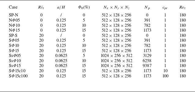


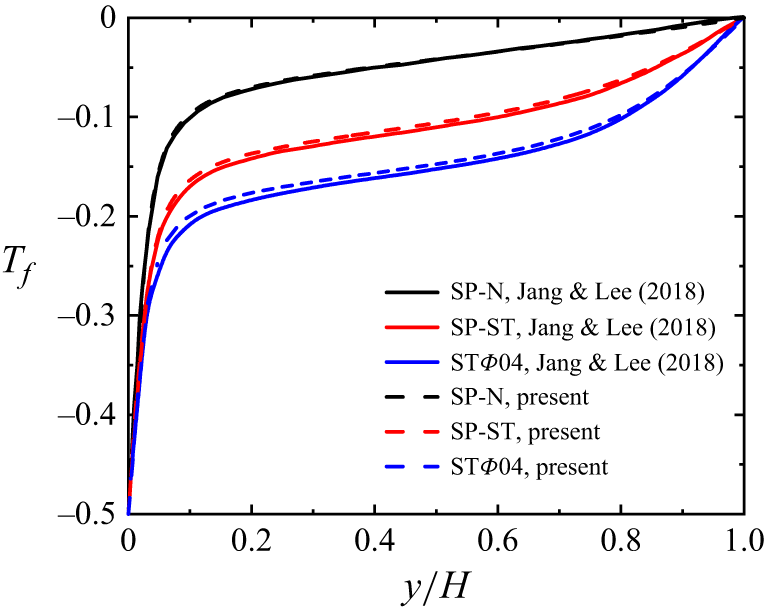


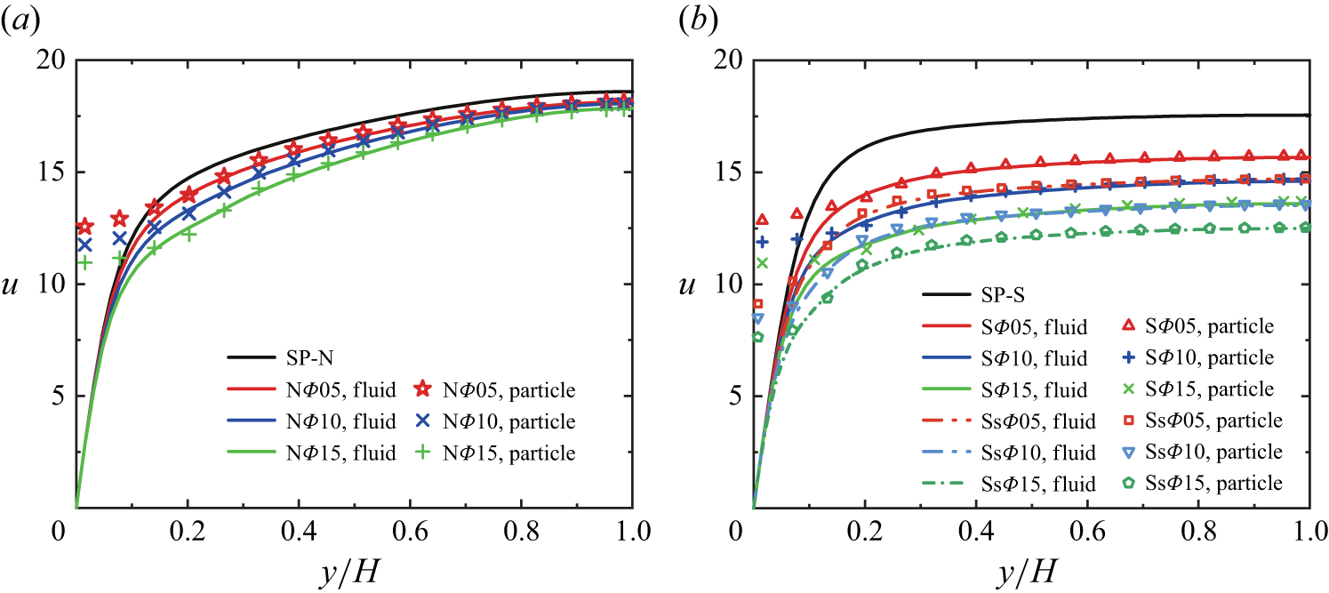


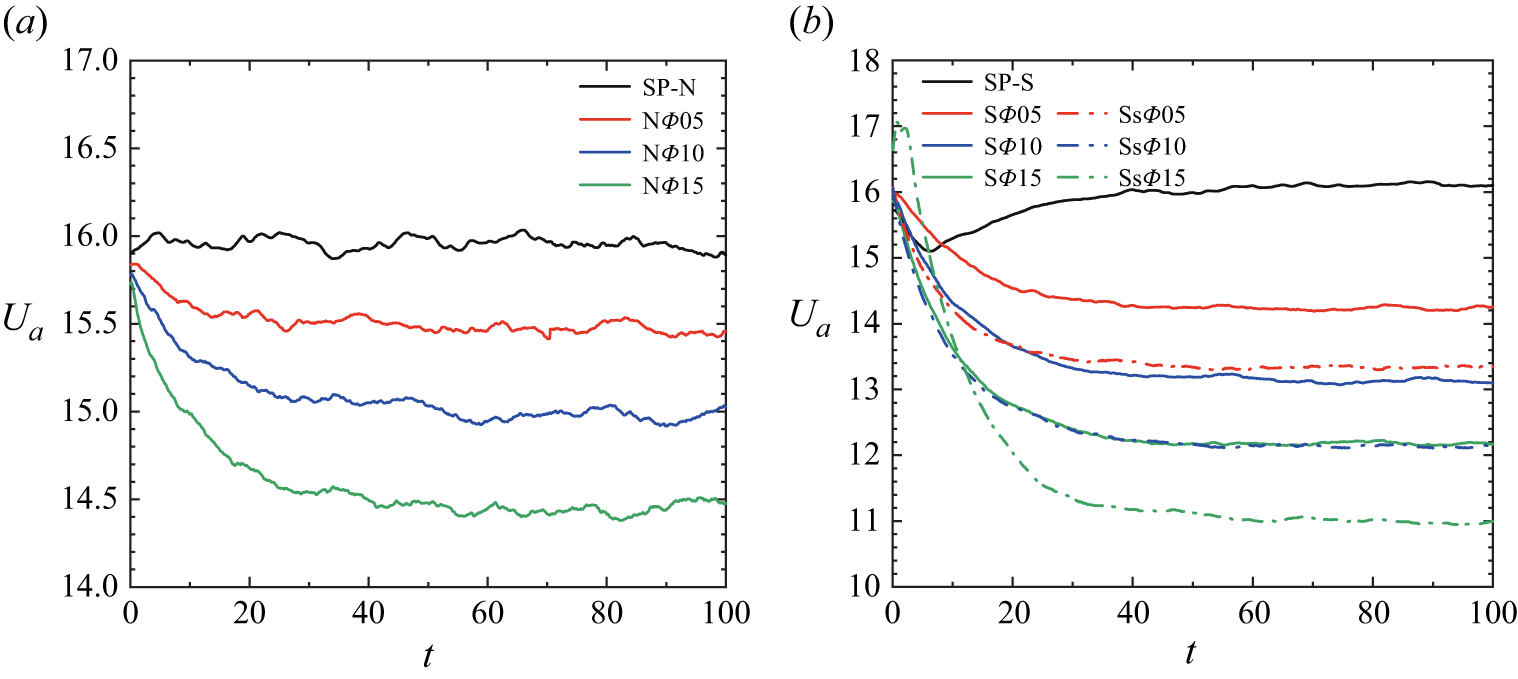


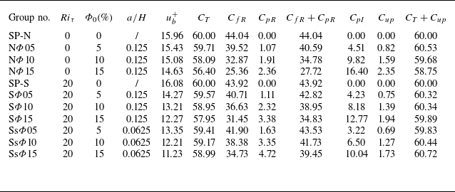


 Open access